Toward Generative Modeling of Calorimetry Signals Exploring adversarial and variational learning of particle physics data By MICHAEL S. ALBERGO DOWNING COLLEGE Department of Physics UNIVERSITY OF CAMBRIDGE A master’s dissertation submitted to the University of Cambridge in accordance with the requirements of the degree of MPHIL IN PHYSICS for the Department of Physics in the School of the Physical Sciences. AUGUST 2018 Supervisor: Dr. Christopher Lester Word count: 14,856

Welcome message from author
This document is posted to help you gain knowledge. Please leave a comment to let me know what you think about it! Share it to your friends and learn new things together.
Transcript

Toward Generative Modeling ofCalorimetry Signals
Exploring adversarial and variational learning of particle physics data
By
MICHAEL S. ALBERGO
DOWNING COLLEGE
Department of PhysicsUNIVERSITY OF CAMBRIDGE
A master’s dissertation submitted to the University ofCambridge in accordance with the requirements of the degreeof MPHIL IN PHYSICS for the Department of Physics in theSchool of the Physical Sciences.
AUGUST 2018
Supervisor: Dr. Christopher Lester
Word count: 14,856


ABSTRACT
Modern particle physics simulations used by ATLAS to model particle detector responsesprimarily rely on computationally expensive monte carlo methods that make incrementalprobabilistic decisions to imitate the behavior of a particle interacting with material. As
the energy or complexity of the interacting material increase and the number of steps or numberof calculations per step rise, these simulations can become exponentially more costly. However,recent advances in deep generative modeling could provide an alternative to this standardby approximating the underlying probability distribution from which these simulated eventsare sampled. It is the purpose of this master’s dissertation to validate proof of concept usinggenerative modeling to accomplish some of the same tasks that modern Monte Carlo Methods(MCMs) are posed with. In this text, I demonstrate the use of Generative Adversarial Networks(GANs) and Variational Autoencoders (VAEs) to model calorimetry signals. This illustrationbegins with simple modeling tasks, such as generating Gaussian and Beta distributions to explorethe validity of different GAN training methods. Later, I apply this to a simple physics landscape,where I use a GAN to learn some of the conditional behavior of the Delphes fast detector simulator.Further, I train both GANs and VAEs to emulate 2d-projections of more complex calorimetrysimulations that match the output of Geant4, and I introduce a conditional Ø-CVAE that usesinformation about the physics event to more selectively simulate the calorimeter signal. In theprocess, I examine the advantages and disadvantages of different architectures and models inhopes of providing a clearer survey of these novel machine learning techniques and their potentialrole in particle physics simulation.
iii


DEDICATION AND ACKNOWLEDGEMENTS
I would like to thank my advisor, Dr. Christopher Lester, for continuously making me thinkmore carefully and analytically about the research at hand, for being accessible at manyan odd hour/timezone, and for being a willful participant in the hunt for securing powerful
computing tools. I’d like to acknowledge John Hill for his consistent help in maintaining suchcomputing tools. I’d also like to thank Nvidia for supplying such computing tools. I would beremiss not to thank Dr. David Lopez-Paz for welcoming me as a distant pupil of his, and forguiding me on how to best use and explore the space of generative models. And lastly, there waspersistent support supplied to me at a distance across the Atlantic from Gal Wachtel and myparents. A very big shout out to them. Happy retirement, Dad. Thank you.
v


AUTHOR’S DECLARATION
This dissertation is the result of my own work and includes nothing which isthe outcome of work done in collaboration except where specifically indicatedin the text.
vii


TABLE OF CONTENTS
Page
List of Tables xi
List of Figures xiii
1 Introduction 11.1 Current simulation techniques . . . . . . . . . . . . . . . . . . . . . . . . . . . . . . . 2
1.1.1 Event generator: Pythia . . . . . . . . . . . . . . . . . . . . . . . . . . . . . . . 31.1.2 Delphes . . . . . . . . . . . . . . . . . . . . . . . . . . . . . . . . . . . . . . . . 31.1.3 Geant4 . . . . . . . . . . . . . . . . . . . . . . . . . . . . . . . . . . . . . . . . . 4
1.2 Machine learning: introduction and application in HEP . . . . . . . . . . . . . . . . 61.2.1 Unsupervised generative models vs discriminative models . . . . . . . . . . 61.2.2 Generative adversarial networks . . . . . . . . . . . . . . . . . . . . . . . . . 71.2.3 Variational autoencoders . . . . . . . . . . . . . . . . . . . . . . . . . . . . . . 9
1.3 Machine learning in high energy physics . . . . . . . . . . . . . . . . . . . . . . . . . 121.3.1 Overview . . . . . . . . . . . . . . . . . . . . . . . . . . . . . . . . . . . . . . . . 12
2 Proof of Generative Modeling Concept: Toy Dataset 152.1 Modeling well defined distributions . . . . . . . . . . . . . . . . . . . . . . . . . . . . 15
2.1.1 Comparing GAN loss function modifications . . . . . . . . . . . . . . . . . . 162.1.2 Model architecture and parameter choice . . . . . . . . . . . . . . . . . . . . 172.1.3 Results . . . . . . . . . . . . . . . . . . . . . . . . . . . . . . . . . . . . . . . . . 18
2.2 Conditional distribution generation . . . . . . . . . . . . . . . . . . . . . . . . . . . . 222.2.1 Task and model architecture . . . . . . . . . . . . . . . . . . . . . . . . . . . . 222.2.2 Results . . . . . . . . . . . . . . . . . . . . . . . . . . . . . . . . . . . . . . . . . 23
2.3 Conclusions . . . . . . . . . . . . . . . . . . . . . . . . . . . . . . . . . . . . . . . . . . . 24
3 Delphes GAN Modeling 273.1 What scenario is Delphes setting? . . . . . . . . . . . . . . . . . . . . . . . . . . . . . 27
3.1.1 Delphes electron Gun . . . . . . . . . . . . . . . . . . . . . . . . . . . . . . . . 303.1.2 CGAN architecture and objective . . . . . . . . . . . . . . . . . . . . . . . . . 31
ix

TABLE OF CONTENTS
3.1.3 Results . . . . . . . . . . . . . . . . . . . . . . . . . . . . . . . . . . . . . . . . . 323.2 Discussion . . . . . . . . . . . . . . . . . . . . . . . . . . . . . . . . . . . . . . . . . . . 36
4 Geant4 GAN Calorimetry Modeling 374.1 Greater complexity: Geant4 and 2D image generation . . . . . . . . . . . . . . . . . 38
4.1.1 2D Computer vision and convolutional Models . . . . . . . . . . . . . . . . . 404.2 DCGAN modeling of calorimeter images . . . . . . . . . . . . . . . . . . . . . . . . . 42
4.2.1 Training data and model architecture . . . . . . . . . . . . . . . . . . . . . . 424.2.2 Results . . . . . . . . . . . . . . . . . . . . . . . . . . . . . . . . . . . . . . . . . 43
4.3 Why not try a fully connected GAN? . . . . . . . . . . . . . . . . . . . . . . . . . . . . 584.3.1 FCGAN architecture and results . . . . . . . . . . . . . . . . . . . . . . . . . 594.3.2 Overall Geant4 GAN discussion . . . . . . . . . . . . . . . . . . . . . . . . . . 64
5 Geant4 VAE Calorimetry 675.1 Bring encoding and stability to generation with variational autoencoders . . . . . 67
5.1.1 What may VAEs improve or hinder? . . . . . . . . . . . . . . . . . . . . . . . 685.1.2 VAE model architecture . . . . . . . . . . . . . . . . . . . . . . . . . . . . . . . 685.1.3 VAE results . . . . . . . . . . . . . . . . . . . . . . . . . . . . . . . . . . . . . . 695.1.4 Conditional generation with VAEs . . . . . . . . . . . . . . . . . . . . . . . . 82
6 Conclusion 876.1 Future improvements . . . . . . . . . . . . . . . . . . . . . . . . . . . . . . . . . . . . . 88
A Appendix A 91A.1 Chapter 1 Notes . . . . . . . . . . . . . . . . . . . . . . . . . . . . . . . . . . . . . . . . 91A.2 Chapter 2 Notes . . . . . . . . . . . . . . . . . . . . . . . . . . . . . . . . . . . . . . . . 92A.3 Chapter 3 Notes . . . . . . . . . . . . . . . . . . . . . . . . . . . . . . . . . . . . . . . . 92A.4 Chapter 4 Notes . . . . . . . . . . . . . . . . . . . . . . . . . . . . . . . . . . . . . . . . 93
B Appendix B 95B.1 Chapter 1 Notes . . . . . . . . . . . . . . . . . . . . . . . . . . . . . . . . . . . . . . . . 95
Bibliography 97
x

LIST OF TABLES
TABLE Page
2.1 Different GAN loss formulations . . . . . . . . . . . . . . . . . . . . . . . . . . . . . . . . 172.2 KL-divergences for different GAN loss paradigms . . . . . . . . . . . . . . . . . . . . . . 192.3 Extrapolating Gaussian generation to mean conditions outside training set . . . . . . 25
3.1 Delphes Gaussian PT smearing widths . . . . . . . . . . . . . . . . . . . . . . . . . . . . 293.2 e° gun parameters . . . . . . . . . . . . . . . . . . . . . . . . . . . . . . . . . . . . . . . . . 303.3 Overall CGAN-Delphes distribution comparisons . . . . . . . . . . . . . . . . . . . . . . 333.4 Comparing ¥ dependence for different energies . . . . . . . . . . . . . . . . . . . . . . . 35
4.1 Geant4 e° gun design . . . . . . . . . . . . . . . . . . . . . . . . . . . . . . . . . . . . . . . 424.2 GAN architecture for 64x64 images . . . . . . . . . . . . . . . . . . . . . . . . . . . . . . 434.3 GAN architecture for 32x32 images . . . . . . . . . . . . . . . . . . . . . . . . . . . . . . 444.4 KL-divergence estimates DCGANs . . . . . . . . . . . . . . . . . . . . . . . . . . . . . . . 44
5.1 KL-divergence estimates VAEs . . . . . . . . . . . . . . . . . . . . . . . . . . . . . . . . . 705.2 Final MSE estimates of reconstruction of Geant4 images by the VAE. . . . . . . . . . . 70
6.1 Event computation time comparison . . . . . . . . . . . . . . . . . . . . . . . . . . . . . . 90
A.1 Hyperparameters tested for learning Gaussian and Beta distributions with a GAN."Disc. updates" refers to ratio of updates to discriminator compared to generator. . . . 92
A.2 Hyperparameters for conditional Gaussian synthesis. "Disc. updates" refers to ratio ofupdates to discriminator compared to generator. GAN-DP ∏ refers to parameter onpenalty term of GAN-DP loss function. . . . . . . . . . . . . . . . . . . . . . . . . . . . . 92
A.3 Hyperparameters tested for conditional Delphes PT smearing. "Disc. updates" refersto ratio of updates to discriminator compared to generator. . . . . . . . . . . . . . . . . 93
xi


LIST OF FIGURES
FIGURE Page
1.1 Geant4 detector and event illustration . . . . . . . . . . . . . . . . . . . . . . . . . . . . . 51.2 GAN schematic. . . . . . . . . . . . . . . . . . . . . . . . . . . . . . . . . . . . . . . . . . . 81.3 Autoencoder compared to variational autoencoder . . . . . . . . . . . . . . . . . . . . . . 10
2.1 Gaussian and Beta distributions . . . . . . . . . . . . . . . . . . . . . . . . . . . . . . . . 162.2 Replicated Gaussian and Beta distributions with GAN-DP . . . . . . . . . . . . . . . . 192.3 Comparing capacity, efficiency, and stability of GAN loss paradigms . . . . . . . . . . . 202.4 WGAN-GP Beta modeling revisited . . . . . . . . . . . . . . . . . . . . . . . . . . . . . . 212.5 Separating conditional generations . . . . . . . . . . . . . . . . . . . . . . . . . . . . . . . 242.6 Extrapolating Conditional Generations . . . . . . . . . . . . . . . . . . . . . . . . . . . . 25
3.1 Delphes detector schematic . . . . . . . . . . . . . . . . . . . . . . . . . . . . . . . . . . . 283.2 Pythia input parameters . . . . . . . . . . . . . . . . . . . . . . . . . . . . . . . . . . . . . 313.3 CGAN for Delphes PT smearing . . . . . . . . . . . . . . . . . . . . . . . . . . . . . . . . 323.4 Distribution metrics for Delphes CGAN . . . . . . . . . . . . . . . . . . . . . . . . . . . . 333.5 Comparing ¥ dependence for overall distribution . . . . . . . . . . . . . . . . . . . . . . 343.6 Comparison of smearing distributions for two separate energies to show that the
implicit condition of PT is taken into account. Top Row: PT for 500 MeV events atdifferent ¥ ranges for both Delphes and the GAN. Bottom Row: Equivalent for 40000MeV events. . . . . . . . . . . . . . . . . . . . . . . . . . . . . . . . . . . . . . . . . . . . . . 35
4.1 3D Geant4 images translated to 2D projections . . . . . . . . . . . . . . . . . . . . . . . 394.2 Comparing average DCGAN calorimeter images 32x32 . . . . . . . . . . . . . . . . . . . 474.3 Difference between GANs and Geant4 average image 32x32 . . . . . . . . . . . . . . . 484.4 Distribution metrics of cross-sections average DCGAN calorimeter images 32x32 . . . 484.5 Cross-Sections of average DCGAN calorimeter images 32x32 . . . . . . . . . . . . . . . 494.6 DCGANs Samples 32x32 . . . . . . . . . . . . . . . . . . . . . . . . . . . . . . . . . . . . . 504.7 Comparing average DCGAN calorimeter images 64x64 . . . . . . . . . . . . . . . . . . . 534.8 Distribution metrics comparison of average DCGAN calorimeter images 64x64 . . . . 544.9 Cross-sectional distribution comparison of average DCGAN calorimeter images 64x64 55
xiii

LIST OF FIGURES
4.10 Difference between GANs and Geant4 average image 64x64 . . . . . . . . . . . . . . . 564.11 DCGANs Samples 64x64 . . . . . . . . . . . . . . . . . . . . . . . . . . . . . . . . . . . . . 574.12 Mode hopping between sequential epochs of average DCGAN-DP energy deposition . 584.13 Visualization of FCGANs for 32x32 and 64x64 images. . . . . . . . . . . . . . . . . . . . 594.14 FCGANs Samples 32x32 . . . . . . . . . . . . . . . . . . . . . . . . . . . . . . . . . . . . . 604.15 Metrics comparison of cross-sections of average FCGAN calorimeter images 32x32 . . 614.16 Cross-sectional distribution comparison of average FCGAN calorimeter images 32x32 624.17 Difference between FCGANs and Geant4 average image 32x32 . . . . . . . . . . . . . . 634.18 FCGANDP cross-section metrics in sequential epochs . . . . . . . . . . . . . . . . . . . 64
5.1 Visualization of VAEs for 32x32 and 64x64 images . . . . . . . . . . . . . . . . . . . . . 705.2 Average Geant4 image vs. average VAE image 32x32 . . . . . . . . . . . . . . . . . . . . 725.3 Distribution metrics comparison of average VAE calorimeter image 32x32 . . . . . . . 735.4 Cross-sectional distribution comparison of average VAE calorimeter image 32x32 . . 745.5 Reconstruction of 6 events by VAE . . . . . . . . . . . . . . . . . . . . . . . . . . . . . . . 755.6 VAE Samples 32x32 . . . . . . . . . . . . . . . . . . . . . . . . . . . . . . . . . . . . . . . . 765.7 Average pixel energy deposition between DCWGAN and VAE models . . . . . . . . . . 765.8 Average Geant4 image vs. average VAE image 64x64 . . . . . . . . . . . . . . . . . . . . 785.9 Analysis of Average VAE image, 64x64 . . . . . . . . . . . . . . . . . . . . . . . . . . . . 795.10 Cross-sectional comparison of Average VAE image, 64x64 . . . . . . . . . . . . . . . . . 805.11 Reconstruction of 6 events by VAE at 64x64 . . . . . . . . . . . . . . . . . . . . . . . . . 815.12 VAE Samples 64x64 . . . . . . . . . . . . . . . . . . . . . . . . . . . . . . . . . . . . . . . . 825.13 Ø-CVAE adoption of conditional information with Ø . . . . . . . . . . . . . . . . . . . . . 855.14 Ø-CVAE Samples with different Ø values . . . . . . . . . . . . . . . . . . . . . . . . . . . 86
xiv

CH
AP
TE
R
1INTRODUCTION
Physicists care deeply about simulation. For particle physicists, such simulation has
myriad purposes – from theoretical exploration to providing a control and validation
technique for interpreting experimental results. The latter is the concern of this thesis.
High energy physics experiments often involve the collision of fundamental constituents of matter,
and then sieving through the prolific and cryptic debris these collisions produce. It is essential to
know how the physical objects that we know exist will behave in these experiments – either as
the source of or as part of this debris – so that, after taking into account these known factors, we
can try to recognize and make sense of what else is left. That is how discoveries are made.
A limiting factor on our ability to simulate all of the types and contexts of events the physics
community is interested in is computational efficiency. These experiments generally involve
millions of collisions that subsequently produce millions of auxiliary particles, whose signal or
lack of signal must be accounted for by detectors in order for the discoveries mentioned above
to be rigorously made. At CERN and for the ATLAS detector, there is continuous investment in
developing updates or alternatives to current simulation methods that can help reduce both the
computational expense of simulation as well as the amount of data processed and produced by it.
Deep learning [1] and the advent of new generative modeling techniques have provided a fresh
1

CHAPTER 1. INTRODUCTION
source of inspiration for tackling research objectives in particle physics. It is the purpose of this
dissertation to explore how these generative models might help mitigate computation and data
processing expenses by ultimately producing the same simulation output, but by avoiding many
of the steps in the middle.
This chapter will give a layout of some current particle physics simulation tools, a discussion of
novel deep generative models and machine learning techniques, and a literature review of their
current uses in particle physics. The two detector simulators of focus in this dissertation are
Delphes and Geant4. Delphes is a fast simulator which is used as an initial tool in this context to
show proof of concept of employing machine learning to recreate the subtle inefficiencies of how a
detector might mis-measure known accurate events. It serves more as a sanity check, as Delphes
already runs efficient simulations. Geant4 is of greater focus, as its complexities and specificity
can make single event simulations take extended times – up to seconds – when you may want to
simulate thousands of events.
A description of the relevant generative models to challenge these detector simulators – generative
adversarial networks (GANs) and variational autoencoders (VAEs) – will follow. GANs were the
main research topic for this dissertation at first, but upon seeing some of their successes and
limitations, VAEs were introduced to see how they compare or improve on these limitations. I
will begin by reviewing the roles machine learning currently plays in particle physics so that it
can be seen how generative models fit into this picture. Finally, I will give an overview of how
and if at all GANs and VAEs are making their way into the field.
1.1 Current simulation techniques
The state-of-the-art of particle physics simulations is currently based on Monte Carlo methods
(MCMs). MCMs bring a probablistic interpretation to deterministic systems by making use of
random sampling [2]. They are ubiquitous in physics research because of their utility in modeling
high dimensional spaces. The underlying mechanism is to draw a set {si}Ni=1 of independent and
2

1.1. CURRENT SIMULATION TECHNIQUES
identically distributed random variables from a high dimensional space S to approximate a target
probability density p(x), and for N large enough, the approximate distribution samples should
model the real sample space [3]. In our context, the kinematics and other physical parameters
of events influence the cross sections of different physics phenomena (e.g. scattering, coupling
vertices, decays, pair-production, etc.) that may occur before and during interaction with a
detector. Since it is not feasible to exactly model the probability distributions behind these (often
quantum mechanical) phenomena, current MCMs used in particle physics take the physical rules
we know and take random probabilistic samples to model the analytically challenging and/or
quantum mechanical aspects of these events. This dissertation will take a look at two simulation
techniques that use MCMs: Delphes and Geant4. The latter would benefit most from speedups,
as this is where the bulk of the Monte Carlo computational complexity arises from.
1.1.1 Event generator: Pythia
To simulate detector responses, one must also generate particles that are shot off to interact
with these detectors. In this work’s usage of Geant4, this process is handled by a subroutine,
but Delphes takes in events that were generated from Pythia. Pythia [4] is a commonly used
particle event generator that can be customized to specify a variety of physical processes and
kinematic parameters, from parton interactions and varying forms of radiation to decays and
hadronisations. The Pythia event creation that is used in this research is merely to generate
electrons at uniformly distributed solid angle with varying energy, which results in a uniform
azimuthal angle and nearly Gaussian pseudorapidity ¥.
1.1.2 Delphes
Delphes [5] is a simple, fast detector simulation package that serves the purpose of fulfilling
rudimentary modeling needs, subject to little customization. The detector is of fixed cylindrical
shape, comprised of calorimeters for electromagnetic and hadronic activity, an inner tracker
3

CHAPTER 1. INTRODUCTION
within and a muon spectrometer as the outer layer. This setup is used to take the Pythia events
generated earlier, which have exactly defined kinematic parameters, and subject them event by
event to the inefficiencies and inaccuracies of a basic detector. This includes instilling a finite
energy E and transverse momentum PT detection resolution in the calorimeters, incorrectly
identifying leptons, smearing the accuracy on the measurement of the location of a detection,
as well as making particle flow and jet reconstructions. While targeting essential detector
functionalities (for example, lepton ID is necessary for recognizing any electroweak event), there
is limited complexity layered on top of this. For instance, photons and electrons only interact
with the electromagnetic calorimeter, while hadrons only interact with the hadronic calorimeter,
which is importantly not true in practice.
Configurations that the user does have control over, however, are the rates of lepton identification
efficiencies and the E and PT measurement resolutions. They can also be conditionally variant,
such that the resolutions are different in different parts of the detector, which is true in
experiment as well. In cylindrical detectors, particles emanating from the center collision point
at high absolute values of ¥ – close to the hypothetical beamline – are more poorly measured
than those more perpendicular to the axis of collision. These types of variations will be explored
in some of the generative models as well.
1.1.3 Geant4
Geant4 [6] is the sophisticated, highly configurable standard for detailed Monte Carlo physics
simulation. In fact, the original paper submitted detailing it has become one of the most cited
paper in nuclear physics and 2nd most cited paper by all of CERN [7]. The software excels in
its breadth and depth, being both widely customizable and capable of emulating most of the
physical phenomena seen in real detectors. Geant4 allows the user to design the shape, function,
and material makeup of a detector, as well which physical processes the particles (whose initial
kinematics you can also define) will undergo upon interacting with the material.
4

1.1. CURRENT SIMULATION TECHNIQUES
The Monte Carlo technique that Geant4 uses is driven by a physics-informed probabilistic
stepping function. A particle is propagated through the simulator in small iterative steps, at each
of which a set of physics rules and constraints inform what subprocesses should occur, such as
phenomena like pair production, multiple scattering, bremsstrahlung, etc. The parameters of
each particle and the event register are subsequently updated to maintain information important
for track reconstruction and event summaries. As the complexity of events increases – such
as by introducing more physics, smaller step sizes, or initial parameters that force a greater
number of subprocesses – the computation cost of this step-wise technique significantly increases.
Moreover, the majority of the internal calculations done by the software might not be relevant to
the endpoint of information that the investigator is interested in, but are necessary interim steps
of the Monte Carlo method to reach those endpoints. This computational expense as well as a
reconsideration of the necessity for some of the calculations that drive the results of the Monte
Carlo method (for certain objectives) motivated the explorations in this work. I seek to probe the
question: can novel machine learning techniques overcome these limitations to achieve the same
objective in more efficient means?(a) (b)
FIGURE 1.1. (a) The example structure of a detector made of a 8mm thick lead sheetand a 75mm thick Polystyrene scintillator. (b) The propagation of an 1800 MeVelectron and its constituent child particles through the detector.
Evidently, the software provides a plethora of detail - a level of specificity that the work in
this dissertation does not seek to emulate. Let us consider a circumstance that will be explored
in this thesis. At the end of an event in which an electron is fired at a detector, Geant4 will
have created and propagated all particles until they drop below a threshold energy, and the full
path of their tracks, identity, etc will have been processed, as shown in Figure 1.1. In certain
instances, researchers are not interested in all of this detail, but rather, for example, how much
and where energy was deposited in the detector in the end. In such a case, being able to sample
5

CHAPTER 1. INTRODUCTION
from the underlying distribution of these energies would be a drastically more efficient means
of simulating the event, without having to propagate all the physics responsible for the signals.
We can imagine this setup for our machine learning applications, where the goal is to learn how
to sample from these energy distributions by treating the depositions as 2D image of fixed size
across the detector space. This is not a new technique, and was developed and applied in other
high energy physics machine learning contexts [8].
1.2 Machine learning: introduction and application in HEP
Machine learning, a subset of artificial intelligence, describes the class of methods for automating
the process of building mathematical models. These models generally learn and update based on
a performance metric – a loss function – of how accurately said models processed data they were
exposed to. Moreover, machine learning focuses on the development of algorithms to complete
specific tasks by generalizing from example [9]. In recent years, technological advancements have
made deep learning, in which artificial neural network layers are stacked in sequence to learn
higher order abstractions of data [1], the state-of-the-art for many machine learning tasks. These
tasks are approached from two perspectives – discrimination and generation – and achieving
these goals is done by unsupervised, semi-supervised, or fully supervised learning paradigms.
This work makes use of unsupervised generative models.
1.2.1 Unsupervised generative models vs discriminative models
One of the major goals of machine learning is to understand the essential parameters explaining
why a dataset is the way it is. Most commonly, this is seen as a problem of building a model that
can learn a probability distribution that discriminates some data from other data. In the case of
functional mapping in which a y is associated to an input x, this means learning a conditional
probability p(y|x), where the likelihood of the output value is predicted given some input condition.
In applicable cases like classification or regression, the goal is to discriminatively ascertain likely
6

1.2. MACHINE LEARNING: INTRODUCTION AND APPLICATION IN HEP
y values for a given x. Other times, when a greater understanding of a functionally mapped space
is desired beyond the distribution of some output conditioned on some input, the goal is to learn
a joint probability p(x,y) – to gain insight into the distribution that is responsible for generating
all the data.
Even more generally, there are many instances when there is no relational mapping or "labeling"
behind the data distribution we are curious about. That is, we are only given some (x1, . . . ,xn)
that are distributed according some probability distribution p(x). In such case, the objective is
to model the true distribution p(x) with some parameterized approximation pµ(x) so that we
can generalize on i) estimating the likelihood of some x in the domain and on ii) making novel
samples that fall under the distribution. Approaches to this problem are detailed below.
1.2.2 Generative adversarial networks
A common dilemma in generative modeling is choosing the right evaluation metric in your training
regime,1 as likelihood calculations on latent variable and energy maximization techniques are
generally intractable to compute [11]. While proxy metrics related to likelihood have been
used instead, a novel training technique known as adversarial training replaces the traditional
likelihood estimation with a trainable network, whose task is to discriminate generated samples
that came from pµ(x) from those of the true p(x). Generative adversarial networks (GANs)
conceived in recent years follow this paradigm [12].
GANs function as a competition between two competing neural networks - a generator and a
discriminator – which are both represented by functions that are differentiable with respect
to inputs and weight parameters. Let the discriminator and generator have trainable network
parameters ¡ and µ respectively. The generator takes in some latent noise vector z and seeks to
output a conditional signal pµ(x|z). The discriminator takes in either the output of the generator
which is a sample from the approximate distribution or a sample from the true distribution and
1See Goodfellow, et al 2016 [10] for further discussion of maximum likelihood approaches in generative modeling.
7

CHAPTER 1. INTRODUCTION
outputs a sigmoid value of the probability that the given sample is real or counterfeit. The two
functions share a cost function V – one that the generator tries to minimize and the discriminator
tries to maximize:
(1.1) minG
maxD
V (D,G)= Ex[ln(D¡(x))]+Ez[ln(1°D(Gµ(z))]
where ¡ and µ are the parameters of the discriminator and the generator, respectively. The
training process on this value function with an optimal discriminator has been shown to be
equivalent to minimizing the Jensen-Shannon divergence [12] given by:
(1.2) DJS = 12
DKL(Preal ||12
(Preal +Pgen))+DKL(Pgen||12
(Preal +Pgen))
for Kullback-Leibler divergence DKL(P||Q)=°Pi P(i) ln P(i)
Q(i) . The ultimate goal is for the generator
to create samples that are coming from an approximate distribution so close to the real distribution
that the discriminator can no longer tell them apart from real samples. It should be noted that
because in real world applications the model does not have access to the full distribution p(x),
the generator can only best learn the training distribution p̂(x).
calculate
discriminate
x
D
generate
z
generateG
discriminate
x'
Loss
update
update
FIGURE 1.2. Learning schematic of GAN.
GANs have become of particular interest in the generative modeling community because of
their ability to model multi-modal output [10], that are subjectively realistic. That being said,
the original GAN model has a number of limitations, and the theory behind them is still being
explored by an eager machine learning community. These limitations could arise from a number
of theoretical problems as detailed in [13]: overfitting, density misspecification, or dimensional
8
1.2. MACHINE LEARNING: INTRODUCTION AND APPLICATION IN HEP
misspecification. GANs are thus susceptible to collapsing on one mode of the data, computing
non-finite gradient updates during backpropagation, or to experiencing vanishing gradients
that fail to significantly update the network parameters. There are improvements to these
shortcomings by changing the objective metric to integral probability metrics [14], applying
regularization on the gradients of the discriminator [13] or on missing data modes [15], combining
regularization with a new objective function [16], or by adding noise to the discriminator input
to create a smoother probability distribution [17] to prevent vanishing gradients. Most of these
methods are examined for their convergence in [18]. Throughout this thesis, I will compare and
select some of these examined methods based on their performance on real datasets. Namely,
I will be comparing the original GAN training metric, the Wasserstein-GAN with a gradient
penalty from [14, 16], and the discriminator gradient penalty approach of [13]. I test these metrics
on controlled datasets to select which to proceed with for more complex simulation later on.
1.2.3 Variational autoencoders
Autoencoding is a machine learning technique that embeds some high dimensional data into a
lower dimensional space [19]. It is used for purposes of dimensionality reduction and structure
learning. That is, one can learn the important features of data by constraining it to a compressed
representation. Variations of this original structure for different encoding or feature learning
functionality have appeared since, such as denoising autoencoders [20], sparse autoencoders
[21], and contractive autoencoders [22]. It was not until recently that a sample-able generative
modeling extension [23] called the variational autoencoder (VAE) was derived.
A conventional autoencoder enforces a deterministic dimensionality reduction on the data.
Generally, the training process involves taking in some x, encoding to a new vector z of lesser
dimensionality, decoding this back to some higher dimensional x0 and computing the mean
square error loss function L = 1n
Pni=0(xi °x0
i)2 to update the network weights. Ensuring that
one can reconstruct the original x using the encoded vector z and a decoding neural network
helps reinforce that important features of the data are captured by the latent space. That being
9

CHAPTER 1. INTRODUCTION
said, there is no continuity enforced on the latent space, just instances of captured variance for
the specific encoding of each input x. VAEs bring a probabilistic reconsideration to the normal
autoencoder paradigm and can introduce a more expressive latent space than point by point
encoding.
In the VAE setting, we take the assumption that our training data {xi}ni=1 is produced by some
latent embedding z so that the true likelihood of any xi is given by p(xi|z). Moreover, we’d like
to be able to generate samples like x based on our encoded samples z. This is decoding like the
normal autoencoder, but now, as stated above, we assume that these new samples of x come
from some distribution that is conditioned on z, known as p(x|z). We try to learn an empircal
approximation of this true distribution based on our training data pµ(x|z), where µ are the
parameters of the neural network doing the decoding. To optimize our generative model, we’d like
to maximize the marginal likelihood – also known as the evidence – of the data by maximizing
(1.3) p(x)=Z
zp(x,z)=
Z
zp(x|z)p(z)
This is just a manifestation of Bayes Theorem and the product rule. We can assume the prior
(a)
(b)
Encoder Network
Decoder Network
FIGURE 1.3. (a) A conventional autoencoder. (b) A variational autoecoder. Notice thatthe addition of the ≤ reparameterization makes the sampling independent of thegraph to ensure that it is still differentiable.
10

1.2. MACHINE LEARNING: INTRODUCTION AND APPLICATION IN HEP
p(z) is distributed N (0,1), and the conditional p(x|z) can be estimated from our decoder network.
However, the integration over all z is generally intractable to compute, so the evidence cannot be
maximized in this form. Instead, we can approximately compute an encoding p(z|x) with some
q¡(z|x) to generate samples of z that can be used to approximate p(x) [24]. With this encoder,
we can derive a lower bound on the log-likelihood of our training data pµ(x) by multiplying by a
constant, and expanding, as explained in [23, 25]:
ln pµ(x)= Ezªq¡(z|x)[ln pµ(x)]
= Ezªq¡(z|x)[lnpµ(x|z)pµ(z)
pµ(z|x)q¡(z|x)q¡(z|x)
]
= Ezªq¡(z|x)[ln pµ(x|z)]°Ezªq¡(z|x)[lnq¡(z|x)pµ(z)
]+Ezªq¡(z|x)[lnq¡(z|x)pµ(z|x)
]
= Ezªq¡(z|x)[ln pµ(x|z)]°DKL(q¡(z|x) || pµ(z))+DKL(q¡(z|x) || pµ(z|x))
(1.4)
The expectation over z equates the last two logarithmic fractions to KL-divergences. The first
term can be estimated through sampling using a reconstruction loss. We can consider the
reconstruction loss term as ensuring that real samples are embedded into the latent distribution
and forcing the decoding function to be an approximate inverse of the encoding function. The
second term calculates the similarity between the encoded distribution q¡(z|x) and a (generally)
Gaussian prior, and the third term is intractable. However, DKL(·||·)∏ 0, so the first two terms
can still function as a differentiable lower bound on the log-likelihood ln pµ(x) – also known as the
also known as the evidence lower bound (ELBO). Because it is differentiable, it can be optimized
to maximize the lower bound of the likelihood.
Graphs of prototypical AE and VAE models are shown in Figure 1.3 to highlight their differences.
An important distinction beyond the different objective function is in the encoding bottleneck.
Instead of encoding down to some single latent representation, a VAE encodes to two bottlenecks –
a mean vector and a variance vector. The latent vector is then created by sampling the mean vector,
the variance vector, and combining these samples with a noise term ≤. This is to permit the VAE
11

CHAPTER 1. INTRODUCTION
to generate new samples while still allowing the graph to be differentiable for backpropagation
optimization and is known as the reparameterization trick. Autoencoders and VAEs are only
cousins because of their encoding and decoding paradigm; otherwise, they are conceptually
(Bayesian vs deterministic) and functionally (reductive vs generative) quite different.
Compared to GANs, VAEs have a tangible likelihood estimator that has a stable form of
optimization. The adversarial optimization approach of GANs, on the other hand, does not
have a clear optimization performance metric (this is an open question in GAN theory). Moreover,
the continuous latent space embedding of the VAE and forcing the encoding distribution to
model its prior could help improve the problem of sample diversity/mode collapse that GANs are
susceptible to. Recent improvements to the VAE model via the Ø-VAE [26] help disentangle the
features in the latent space so they can be conditionally independent and better interpolated.
This will be explored in testing later on. That being said, using a likelihood estimator in the VAE
that is based on conventional sampling (like a mean squared error reconstruction) could put an
upper limit on the resolution quality of the samples, something VAEs are known to suffer from.
1.3 Machine learning in high energy physics
1.3.1 Overview
Evidence of machine learning in high energy physics extends all the way back to 1987 [27]. Since
then, there has been a recent proliferation of research employing novel model learning machinery
in both theory and experiment. Researchers have put constraints on perturbative theories [28]
and generalized SUSY exclusion criteria from experiment [29]. Moreover, improvements on
experimental data analysis and classification [30, 31] even in semi-supervised regimes [32],
smarter triggering [33], and even searches for new physics [34] have employed machine learning
techniques. Recent developments have also shown proof of concept on using GANs to simulate
energy depositions from a calorimeter [35, 36] and orienting the underlying GAN architecture
12

1.3. MACHINE LEARNING IN HIGH ENERGY PHYSICS
for physics application. They extend previous calorimetry imaging and preprocessing techniques
for jet imaging [37], and builds on other progress in applying deep learning to jet classification
[8, 38] and jet recombination [39] problems.
In this thesis, I will try to validate some of the results achieved in simulating calorimetry images
with a number of circumstances that scale in complexity. I will test GANs out on toy datasets that
are well controlled and choose optimal training paradigms to proceed with. I will explore how well
conditional kinematics can be used to alter the scale and resolution of detector measurements
based on where in the detector events occur much like Delphes does. After this, I will use this
insight to reproduce similar results to [35] using a deep convolutional GAN (DCGAN). In the
process, I will examine some of the limitations of previous models, such as those tied to the
sparsity of the particle showers.
Importantly, I will also introduce a variational autoencoding generative model that provides
strong calorimeter image sample diversity in comparison to where the GAN may falter, and does
so under a more reliable and stable training regime – without convolution – with a latent space
that is less likely to fail to express the breadth of the distribution. This model is also accepting of
conditional information about the desired particle shower generation, as done in [36], with some
caveats. By increasing the pixel resolution in both cases compared to previous work on this topic,
one can exacerbate the impact of sparsity on capturing features of the images. I will present some
evidence that the limitations in convolutional GANs can be improved with fully connected VAEs,
and that these stabler techniques might be more appealing from a practice research perspective.
13


CH
AP
TE
R
2PROOF OF GENERATIVE MODELING CONCEPT: TOY DATASET
In adopting or creating any new mathematical tool, it is important to test its functionality
on controlled circumstances where expected behavior can be closely modeled. While this
mindset is adopted for the entirety of the thesis, I will start from the ground up to validate
and select variations of GAN training regimes. As a first set of tests, I will explore how well GANs
can learn well-known distributions and which learning paradigm does so most efficiently and
stably. Further, I will test the extent to which conditional information can be provided about these
distributions to influence the outcome of the generation process, as well as if this conditionality
is generalizable beyond the range of conditional values the GAN was trained on.
2.1 Modeling well defined distributions
As stated earlier, the input to the conventional GAN model is some arbitrary noise sample z which
can come from a number of distributions, but is generally Gaussian z ª N (0,1) or uniformly
zª unif(0,1) distributed. Given some real distribution p(x) and through the adversarial training
process, the generator should be able to engineer samples using the input noise that emulate data
15

CHAPTER 2. PROOF OF GENERATIVE MODELING CONCEPT: TOY DATASET
coming from this true distribution. If such is the case, this should be approximately empirically
and quantitatively verifiable on some well known distributions such as a N (µ,æ) and Beta(Æ,Ø):
fN (x)= 1p
2ºæexp(° (x°µ)2
2æ2 )
fBeta(x)= 1B(Æ,Ø)
xÆ°1(1° x)Ø°1(2.1)
Both of these have analytically known probability density functions and well recognized sample
distributions, as shown in Equation 2.1 and Figure 2.1:
�3 �2 �1 0 1 2 30
200
400
600
800
1000
1200
Gaussian N (0, 1)
˙�0.2 0.0 0.2 0.4 0.6 0.8 1.0 1.2
0
200
400
600
800
1000
Beta (0.6, 0.6)
Figure 2.1: 10000 samples of Gaussian and Beta distributions. These are the two distributions tobe replicated.
Moreover, using these simple distributions also allows for controlled comparison of different GAN
training methods that employ modifications of the standard loss function. Two distributions were
included to ensure that the way the GAN behaves is actually modeling the distributions rather
than say, behaving poorly in a way that may look like a distribution (if, for example, it were just
inaccurately guessing the mean of the Gaussian such that the inaccuracies looked like standard
deviated sampling).
2.1.1 Comparing GAN loss function modifications
To proceed with the optimal training paradigm on more complex learning problems later, three
different GAN loss function variations were tested for convergence, both in accuracy and efficiency.
16
x
x
count
count
2.1. MODELING WELL DEFINED DISTRIBUTIONS
The three tested are the original GAN proposal [12], the Wasserstein GAN with its improved
training methods [14], and the method of penalizing the gradient of the discriminator when
shown real data as described in [13]. I will refer to the last method as the GAN-DP (discriminator
penalty). The latter two seek to stabilize local training stability. GAN-DP regularizes the original
loss function to maintain steady approach and proximity to Nash equilibrium, and the WGAN-GP
uses regularization and the Wasserstein metric to reformulate the loss as a distance measure
between the real and fake distributions. In such case, the conventional discriminator which
outputs a probability between 0 and 1 that the data came from the real distribution is replaced
with a new network that functions as a more general critic, outputting a real-valued score
associated with the realness of the input sample. Through updating its parameters, the critic
learns a 1-Lipschitz continuous function f . A gradient penalty is included to help enforce the
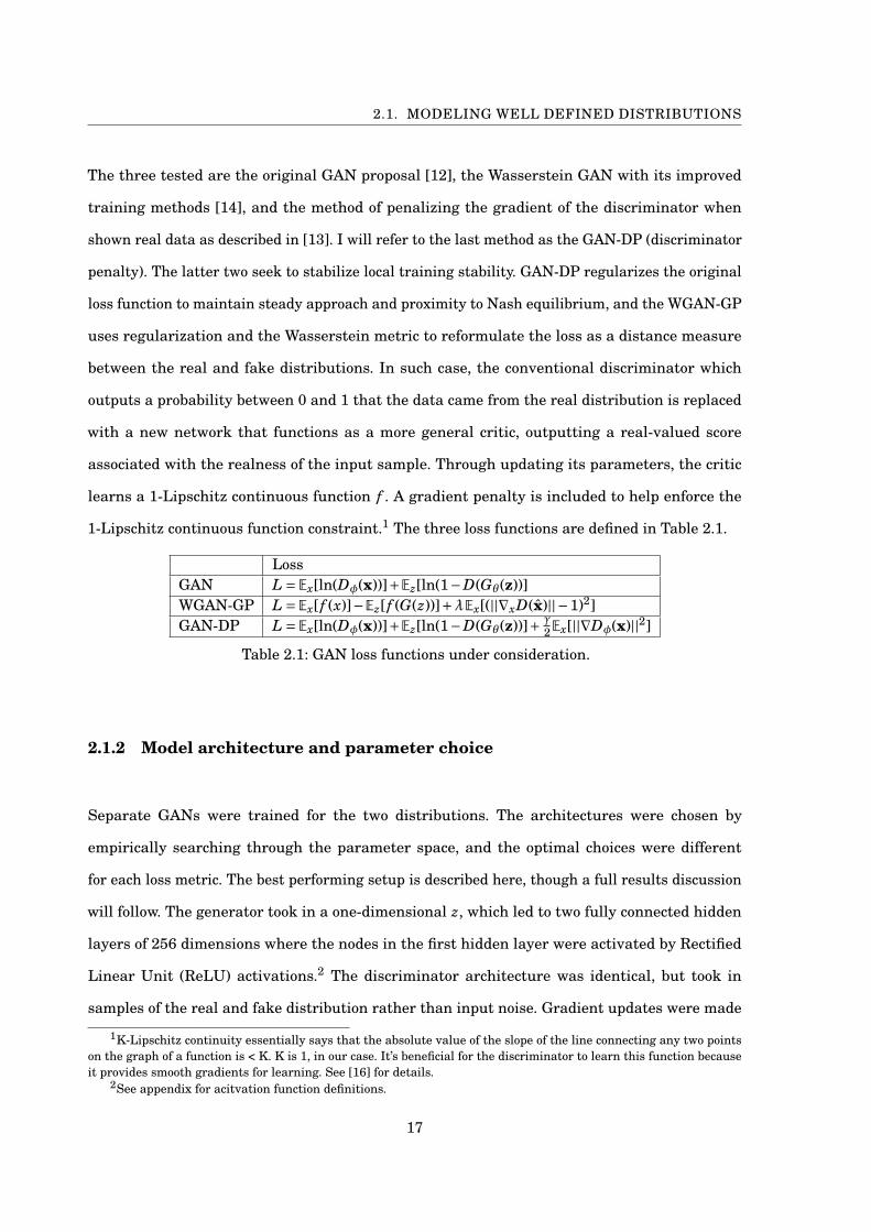
1-Lipschitz continuous function constraint.1 The three loss functions are defined in Table 2.1.
LossGAN L = Ex[ln(D¡(x))]+Ez[ln(1°D(Gµ(z))]WGAN-GP L = Ex[ f (x)]°Ez[ f (G(z))]+∏Ex[(||rxD(x̂)||°1)2]GAN-DP L = Ex[ln(D¡(x))]+Ez[ln(1°D(Gµ(z))]+ ∞
2Ex[||rD¡(x)||2]
Table 2.1: GAN loss functions under consideration.
2.1.2 Model architecture and parameter choice
Separate GANs were trained for the two distributions. The architectures were chosen by
empirically searching through the parameter space, and the optimal choices were different
for each loss metric. The best performing setup is described here, though a full results discussion
will follow. The generator took in a one-dimensional z, which led to two fully connected hidden
layers of 256 dimensions where the nodes in the first hidden layer were activated by Rectified
Linear Unit (ReLU) activations.2 The discriminator architecture was identical, but took in
samples of the real and fake distribution rather than input noise. Gradient updates were made
1K-Lipschitz continuity essentially says that the absolute value of the slope of the line connecting any two pointson the graph of a function is < K. K is 1, in our case. It’s beneficial for the discriminator to learn this function becauseit provides smooth gradients for learning. See [16] for details.
2See appendix for acitvation function definitions.
17

CHAPTER 2. PROOF OF GENERATIVE MODELING CONCEPT: TOY DATASET
using Adam optimization [40] over batches of 256 samples. Training was done over 1000 epochs.
ReLU activations were included to help map any nonlinearities in the transformations between
the noise distribution and the intended real distribution for the generator and to provide this
same flexibility to the discriminator.
The optimal dimensionality of the hidden layers, as well as the learning rate and batch size,
were chosen by hyperparameter tuning, iterating through different combinations of parameters
as defined in Table A.3 in the appendix. Decision criteria for selecting the optimal parameter
were based in training stability and comparison of known distribution parameters like the
full-width-half-maximum (FWHM) and mean of the samples. While these metrics are not fully
expressive of distribution matching and the training stability also depended on the choice of loss
function, they provided empirical evidence of training accuracy. These hyperparamter searches
were performed separately for each of the three loss metrics. Additional hyperparameters appear
in the WGAN-GP and GAN-DP, both of which are tuning values on the magnitude of the gradient
penalties they employ. These were also iterated over in the combination of potential parameters
for optimal training, and the tested values were taken from the original papers explaining the
methods. To supplement these metrics, the KL-divergence – a measure of the distance between
two distributions – was calculated between samples of the real and fake distributions as well.
Moreover, the purpose of this initial section is to show proof of concept in continuing with
these approaches to simulation, so the standard was to show some threshold of feasibility, not
necessarily to give too much attention to optimizing the learning of these toy datasets.
2.1.3 Results
The GAN, WGAN-GP, and GAN-DP training paradigms all showed some capability of learning
these distributions, but the accuracy ands stability of training was optimal under the GAN-DP
process. Exemplary results for the GAN-DP are shown in Figure 2.2. This corroborates theoretical
results outlined in [18], which concluded that WGAN and its variations like (WGAN-GP) do not
always locally converge to Nash-Equilibrium, but zero-centered gradient methods like that in the
GAN-DP do.
18

2.1. MODELING WELL DEFINED DISTRIBUTIONS
˙
Figure 2.2: Example of replicated Gaussian and Beta distributions made by sampling bestgenerators 1000 times. Training was done using the gradient penalty on the discriminator, theGAN-DP learning paradigm.
Results are summarized in Figure 2.3 for the three different training methods with best
performing hyperparameters from the table in Appendix A.2. Each row of Figure 2.3 corresponds
to one of the training methods, and includes sample learned Gaussian and Beta distributions,
followed by the sample mean and standard widths of the distributions across training epochs.
Under the GAN-DP method, the mean and FWHM of the distributions were quickly learned
and close approximation of the distributions was maintained throughout the rest of the training
process. Moreover, empirical samples from the generator have fewer artefacts that deviate from
the normal characteristics of both the Gaussian and Beta distributions. The unregularized
GAN and WGAN-GP show less stable training, deviating from the mean and widths of the true
distributions more often and more poorly approximating these metrics throughout. The artifacts
seen on them could be symptomatic of known issues with these training methods – mode collapse
for the GAN and poor enforcement of the Lipschitz constraint of the WGAN-GP.
Gaussian KL Beta KLGAN 0.82 0.28WGAN-GP 1.09 0.73GAN-DP 0.52 0.11
Table 2.2: Comparison of average KL divergence over 10000 samples generated 100 times forboth the Gaussian and Beta distributions.
It is important to note that the displayed sample distributions are a subjective measure of
19

CHAPTER 2. PROOF OF GENERATIVE MODELING CONCEPT: TOY DATASET
Figure 2.3: Top Row: Generation of Gaussian and Beta distributions using original GAN loss.Middle Row: Generation of Gaussian and Beta distributions using WGAN-GP loss. Bottom Row:Generation of Gaussian and Beta distributions using GAN-DP loss. The right half containsvalues of the sample mean and standard widths of the two generated distributions across epochscompared to ground truth.
accuracy, both due to my selecting of sample distributions to display and due to the stochasticity
of sample generation. Yet, the continuous comparison of some metrics that characterize the
Gaussian and Beta distributions across training epochs allows for more formative evaluation
between the models. The WGAN-GP and unregularized GAN showed evidence of deviating from
expected characteristics even after approximating them better in previous epochs, while the
GAN-DP does not show such inconsistencies. Upon closer inspection of the WGAN-GP results, in
20
GAN
WGAN-GP
GAN-DP

2.1. MODELING WELL DEFINED DISTRIBUTIONS
which the training in the Beta case seems to be converging but at a much slower rate, another test
was done with minute learning rate of 10°5 which was outside of the original hyperparameter
search. Results show that the WGAN-GP could move down the loss surface more stably if
trained with very small gradient updates, as shown in Figure 2.4.3 Moreover, a comparison of the
KL-divergences between estimates of the probability distributions from the generated samples
and the true samples corroborates these claims. The average KL-divergences over 100 samples
of 10000 values each were lowest for the GAN-DP and higher for the unregularized GAN and
WGAN-GP models on both the Gaussian and Beta tests, as shown in Table 2.2. The WGAN-GP
value improved significantly to 0.024 when training was locally convergent in the slow learning
rate case. The KL-divergence was computed by creating normalized histograms of the 10000
values so that there could be a density estimates pGAN (x) and qtrue(x) at each bin. A Kernel
Density Estimation was also tested to compare to the normalized histogram binning technique
and it yielded similar results.
˙
Figure 2.4: WGAN-GP training only achieves accuracy with small learning rate and many epochs.
Overall, the GAN-DP method could accurately model both the Gaussian and Beta distributions,
capturing natural parameters of the distributions. It empirically struggles to generate values
3See Appendix B.1 for comparison of local stability across learning rates.
21

CHAPTER 2. PROOF OF GENERATIVE MODELING CONCEPT: TOY DATASET
at many (º 3) standard deviations from the mean, but this is a marginal inaccuracy. The
WGAN-GP and unregularized GAN empirically and quantitatively show some ability to model
general characteristics of the two distributions, but do so less predictably and less precisely. The
WGAN-GP paradigm shows good potential for success when training in a locally stable regime,
though this might prove inefficient if training remains fragile.
2.2 Conditional distribution generation
Given evidence of GANs’ capability of modeling simple distributions, a natural next test is to
see how well the model can use additional information to modify what it generates. Showing
such would demonstrate how conditional information about, for example, a physics event, could
be used by a single model to generate different corresponding outcomes. Under such conditions,
the generator could be told to, say, develop physics events at varying different energies or
scattering angles, rather than having a separate generator trained to approximate the probability
distribution for each energy and angle. This would of course be tedious and computationally
taxing.
To build on the generation of Gaussians, I now test the same GAN model but now also provide
both the generator and discriminator with conditional information about the mean of the intended
distribution. This is a slight, but potentially powerful modification to the model, one that has
been tested in literature [41] and even already applied in GAN shower generation [36]. I will use
it to show how conditionality can be used on other detector tasks, like correlating shower location
with energy measurement resolution.
2.2.1 Task and model architecture
A conditional GAN-DP with architecture equivalent to the optimal setup chosen in Section 2.1.3
is used. An input noise z ªN (0,1) and a mean condition – one value from [0,5,10] – are supplied
22

2.2. CONDITIONAL DISTRIBUTION GENERATION
to the generator. All hyperparameters can be found in Appendix A.2 again. A faster learning rate
of 0.008 was used this time to see if more efficient training could occur.
The outputted value and the original mean are fed to a discriminator of equivalent architecture as
the previous section. The goal is to have the generator produce Gaussian samples at the specified
mean and only at the specified mean - not having it, for example, produce a value around 5, but
only when conditioned on zero. One to one correspondence is desired. Otherwise, the GAN would
not selectively be making use of the conditional parameter, but rather learning to sample from a
more widespread set of Gaussian values. Further, it is of interest to see that the generator can
extrapolate to create samples of Gaussians around means it was not trained on. Such a quality is
sought after for flexibility, in which, for example, an ATLAS physicist does not need to train a
model on all possible values across a spectrum of a condition like the energy of a collision but
would still be able to sample across such a spectrum.
2.2.2 Results
The conditional GAN model had little trouble learning to sample from the Gaussians centered
at the means it was trained on, and it could generalize to means that were both outside of its
training set and orders of magnitude greater. The generator used the mean as it should, only
generating values around the provided mean and no other, as evidenced in the top half of Figure
2.5. An empirical mean µ̂ and standard deviation æ̂ were calculated for distributions of 10000
generated samples, which were within 8% and 18% of their true values, respectively. The model
was then validated on conditional means it was not exposed to during training. Such scalability
was robust up to conditional information more than 2 orders of magnitude greater than the
training conditions. These values were not normalized during training nor were they during
validation, and where the accuracy of the generation began to falter at around µ= 200 might
be due to the different scales of values in the generator at such point. This is evidence that the
conditional information is not perfectly and independently utilized as a scaling factor for where
23
CHAPTER 2. PROOF OF GENERATIVE MODELING CONCEPT: TOY DATASET
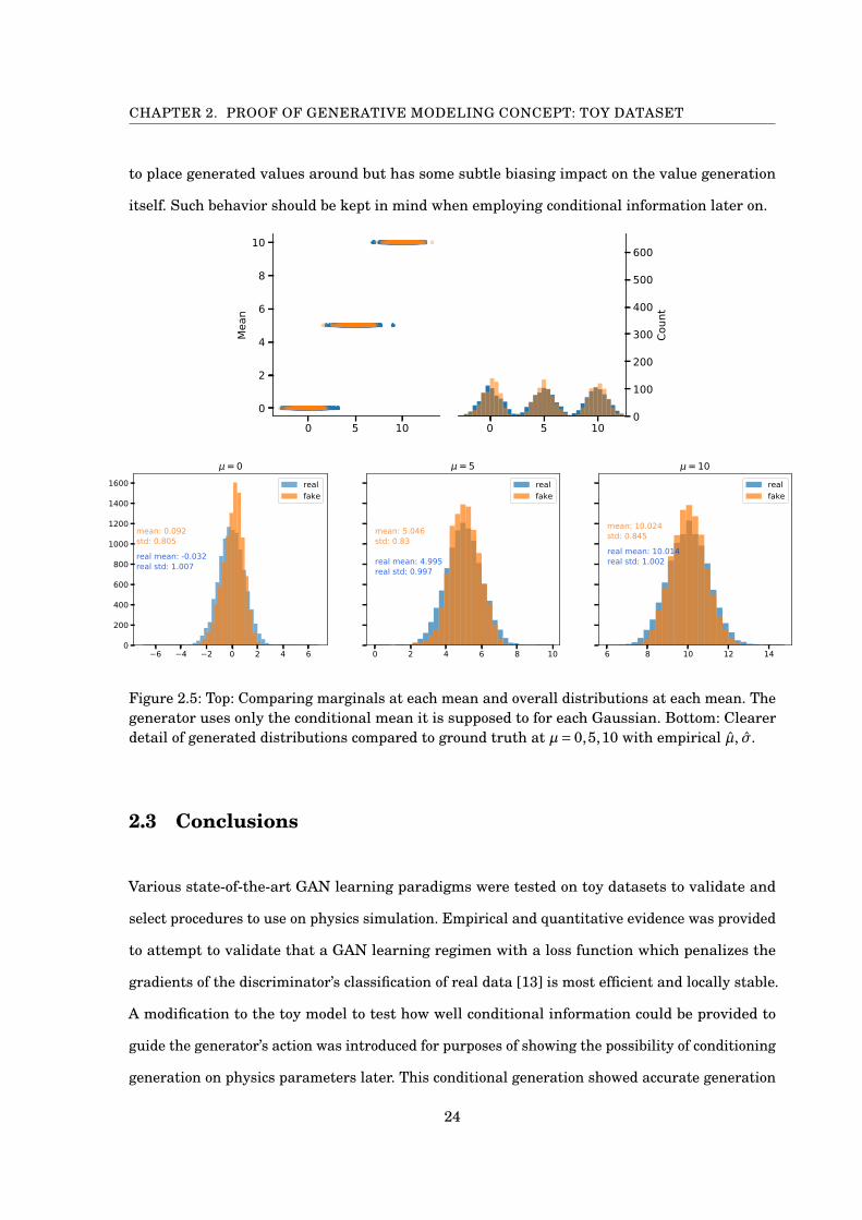
to place generated values around but has some subtle biasing impact on the value generation
itself. Such behavior should be kept in mind when employing conditional information later on.
Figure 2.5: Top: Comparing marginals at each mean and overall distributions at each mean. Thegenerator uses only the conditional mean it is supposed to for each Gaussian. Bottom: Clearerdetail of generated distributions compared to ground truth at µ= 0,5,10 with empirical µ̂, æ̂.
2.3 Conclusions
Various state-of-the-art GAN learning paradigms were tested on toy datasets to validate and
select procedures to use on physics simulation. Empirical and quantitative evidence was provided
to attempt to validate that a GAN learning regimen with a loss function which penalizes the
gradients of the discriminator’s classification of real data [13] is most efficient and locally stable.
A modification to the toy model to test how well conditional information could be provided to
guide the generator’s action was introduced for purposes of showing the possibility of conditioning
generation on physics parameters later. This conditional generation showed accurate generation
24

2.3. CONCLUSIONS
Figure 2.6: Comapring marginals at each mean and overall distributions at each mean. Thegenerator uses only the conditional mean it is supposed to for each Gaussian.
µ 0 5 10 20 40 60 80 100 200KL-div 0.108 0.142 0.072 0.047 0.045 0.052 0.053 0.095 0.206
Table 2.3: Top: 10000 samples of GAN-DP for 6 different conditional means compared to realGaussians. Bottom: Estimated KL-divergences between the real sample and the GAN at trainingand validation means. The GAN was only trained on the first three.
even on conditions scaled to be far different from those the GAN trained on, but the extension of
usable conditional values along the scale did not extend ad infinitum. The choice of conditional
training data should be made cleverly to sample a wide window of potential conditions of interest
to more properly cover the space.
It should be kept in mind that, as with most deep learning analyses, the success of a model
architecture or training processes on one dataset may not easily translate to others of different
character. The compounding factors – from normalization, choice of activation functions, regularization,
network dimensionality, learning rate, etc. – can have significant individual impact and can
combine differently in varying contexts. It is under this mindset that the WGAN-GP will be
tested out on 2D image generation in Chapter 4 even though it showed some limitations here
because it may prove to be more stable in light of novel challenges that may arise. A more
tentative but optimistic takeaway of the presented information might be: "this way can work to
this extent, but there may be other optimal choices to be made in other circumstances."
25


CH
AP
TE
R
3DELPHES GAN MODELING
This chapter examines how the results of the preceding one can be used to continue
the narrative of exploring generative modeling in particle physics detector simulation.
Using Delphes as the representative simulator to emulate, we can begin modeling
the distributions of detector inaccuracy. That is, the goal of this chapter is to show that some
of the fundamentals of a common detector’s behavior, specifically how and why it might make
slight mis-measurements of a particle’s kinematics, can be captured and controlled by generative
adversarial networks. Under these circumstances, multiple conditional directions will be provided
to a GAN to model more complex (or less standardly parameterized) distributions – distributions
that arise from the prescribed directions given to Delphes about how a detector should misbehave.
This is the first step in bringing the tools verified in Chapter 2 to life in a particle physics context.
3.1 What scenario is Delphes setting?
Delphes is a reliable first role model for GANs to replicate in the game of detector simulation
because it propagates a well-controlled, reasonably simple set of statistical rules in a commonly
recognized detector scenario. It seems necessary to frame what prototypical scenario this fast
27

CHAPTER 3. DELPHES GAN MODELING
simulator stages to have a clear sense of what the desired behavior of the GAN is and how we
can check to make sure it acts accordingly. Delphes imagines a cylindrical detector made of: an
inner tracker, electromagnetic (ECAL) and hadronic (HCAL) calorimeters, a muon spectrometer
that includes endcaps on the sides. This is shown in Figure 3.1, as adapted from [42]. A more
detailed description of the most up-to-date scripts and criteria Delphes can make use of can be
found in [5].
Tracker
Calorimeter
Muon Spectrometer
End Caps
FIGURE 3.1. A schematic of Delphes detector setup derived from [42]. Angles that helpdefine the space and are relevant to conditional momenta smearing are presentedfor clarity later.
Two space-defining variables that will be used in this setup are the azimuthal angle ¡ rotated
around circular cross-sections of the cylinder and the pseudorapidity ¥. The pseudorapidity is a
scaled measure of the angle at which the particle travels from the beamline. It is a transformed
measure of the polar angle µ which is 0° along the beamline and 90° perpendicular to it:
¥=° lntanµµ
2
∂(3.1)
This allows ¥ to asymptotically approach infinity as the trajectory becomes parallel with the
beamline. Pseudorapidity is a variant of a commonly employed relativistic measure in physics
28

3.1. WHAT SCENARIO IS DELPHES SETTING?
known as rapidity, which is useful in particle physics to study collisions that occur along a
beamline. Rapidity in experimental particle physics is defined as:
y= 12
lnµ
E+ pzcE° pzc
∂(3.2)
where z is the direction along the beam axis. This expression has a simple Lorentz-transformed
representation, and the difference between rapidity measures in separate reference frames along
the beam axis is zero – boosts along this axis have Lorentz invariant rapidity. An issue with this
variable, though, is that measuring the energy and momentum of a highly energetic particle
is experimentally difficult. Because this conventional rapidity in particle physics depends on
both of these variables, a widely used substitute for this measure that is equal to rapidity in the
relativistic limit is pseudorapidity, which can be written to depend only on µ as seen in equation
3.1. Together, ¥ and ¡ provide two Lorentz-invariant coordinates for collider physics like that at
the LHC.
Table 3.1: Gaussian widths of Delphes PT
mis-measurement in tracks.
Tracks Gaussian Width
0< |¥| < 0.5q
(.03 MeVc )2 +P2
T · (1.3 ·10°2)2
0.5< |¥| < 1.7q
(.05 MeVc )2 +P2
T · (1.7 ·10°2)2
1.7< |¥| < 2.5q
(.15 MeVc )2 +P2
T · (3.1 ·10°2)2
ECAL Tower Gaussian Width
|¥| < 3.2 æEE = .101p
E©0.0017
Delphes also incorporates realistic technological
limitations associated with these variables.
For a detector like ATLAS, the end caps,
which cover areas at high |¥|, have a
high concentration of many, often less
significant particles interact with them, and
measurement resolutions are poorer in this
zone. That is, significant and more analyzable
events generally have more of their momenta
in the transverse plane of the detector, where there are also fewer pieces of debris from messy
and inconsistent interactions that come from the initial sea and valence quark collisions inherent
to proton-based colliders.
I try to replicate some of this behavior by using a Delphes configuration which weakens the
momentum measurement resolution with increasing ¥. Delphes does this by applying a Gaussian
29

CHAPTER 3. DELPHES GAN MODELING
smear to the momentum, and the width of such Gaussian is often calculated as a weighted sum of
resolution limitations in the tracks and in the ECAL (though this is configurable in the Delphes
configuration card). The severity of the mis-measurement is piecewise correlated with ¥ and
continuously correlated with PT and E according to Table 3.1.1 In the weighted sum, the track PT
mis-measurement dominates. Note that as ¥ increases for generated particles at a fixed energy,
their PT will simultaneously decrease, as the majority of the momentum of the particle will be
more closely aligned with the beamline and not in the transverse plane. So, even though the
Delphes tracker will make larger fractional mis-measurements on the PT for higher ¥, the overall
magnitude of those PT values will be smaller, and the smearing will look small accordingly.
3.1.1 Delphes electron Gun
The prototypical physical problem that was chosen to be modeled was a simple electron gun that
fires under the following conditions: a uniformly selected µ and ¡ with energy randomly sampled
from a logarithmically decaying function, as defined in Table 3.2.
Table 3.2: Parameters of e° gun.
cos(µ) Unif[°1,1]
sin(µ)p
1°cos(µ)2
¡ 2 ·º ·Unif[°1,1]
E 10(1+(log10 Emax°1)·Unif[0,1])
Pq
E2 °m2e
Figure 3.2 shows aggregate histograms over 500,000 events
of relevant kinematic variables defined or derived from
the sampled parameters. For electrons, Delphes follows the
protocol above of splitting the PT mis-measurement as the
weighted some of the ECAL and tracking behavior.2 The
energies of particles used in the experiments to follow are low
such that the PT mis-measurement is predominantly from
tracks. That way, the only significant conditional variables
at play come from the PT conditions defined in Table 3.1 rather than from those based on the
ECAL tower as well.1The © symbol in the energy mis-measurement means add in quadrature how it is written for the PT . This was
written as such for the experimental physicists in the house.2Note: While ECALs reconstruct kinetic energy, one can make a robust approximation of PT by calculating
PT = |P|cosh¥ º E
cosh¥ where one assumes E º P by ignoring the rest mass of the particle.
30

3.1. WHAT SCENARIO IS DELPHES SETTING?
FIGURE 3.2. Ground truth distributions of electron gun kinematics for 500,000 events.
3.1.2 CGAN architecture and objective
The objective of our learning paradigm is to supply the GAN with a subset of the same information
Delphes uses to produce an equivalent output of how mis-measurements of the PT of the electron
are distributed. That is, we want the GAN to generate values of PtrueT °Psim
T , the extent of
disagreement between the two values. The conditional GAN (CGAN) takes in a random noise
sample z along with the PT , ¥, and ¡, and the generator outputs a Pdi f f ,GANT in an attempt
to convince the discriminator it is producing samples from the distribution of the difference
between the true PT and the detector’s measurement of the PT . I will call this Pdi f f ,Del phesT .
The discriminator takes in these real or fake values as well as the three conditional variables
(PtrueT ,¥,¡) to judge the authenticity of the samples. This revised model is pictorially represented
in Figure 3.3.
Both the input data to the generator (¥,¡,PtrueT ,z) and the Delphes data (¥,¡,Ptrue
T ,Pdi f f ,Del phesT )
were normalized between (-1, 1) to ensure variables with larger magnitudes of variation like PtrueT
did not over-influence the training criteria. The generator was comprised of two hidden layers of
128 dimensions, separated by ReLU activation, with a final tanh activation at the end to maintain
normalization. The discriminator is analogously structured but with a sigmoid activation on
the last layer. Batches of 64 samples were used to train the model, and ultimately again the
GAN-DP loss paradigm was employed after hyperparameter searching. Complete details on
31

CHAPTER 3. DELPHES GAN MODELING
OR
˙
Figure 3.3: Left: Conditional GAN model for Delphes PT smearing. Right: Delphes PT smearing.
training parameters can be found in Appendix A.3.
3.1.3 Results
Overall sample distributions as well as conditional sample distributions were compared and
analyzed to probe the efficacy of replicating the behavior of Delphes. In general, the CGAN
framework could meet the desired objectives set out, though the training process required slower
learning rates than on the previous simpler sample distributions. Table 3.3 shows a comparison
between the Delphes smearing and the generator smearing, as well as a normalized version of it
to show fractional difference. The distributions empirically show high level of correspondence and
demonstrate low KL-divergence estimates, indicating high similarity in the sample distributions.
This is corroborated by the results in Figure 3.4, for which the full width half maximum, mean,
and kurtosis of the distribution are ultimately approximated by the generator. Note that the
kurtosis is a less exact value to estimate because it is the fourth moment of the distribution. As
such, slower convergence and more noise in this measurement was expected.
Moreover, while there is variation on the estimate of the mean of the distribution, note that this
scale is on the order of 10% of the width of the distribution - a distribution which is narrow to begin
with. As such, the mean is found quickly and only slightly varies around this center across epochs.
32

3.1. WHAT SCENARIO IS DELPHES SETTING?
Unnormalized Normalized byp||PT ||
KL-div 0.163 0.127
TABLE 3.3. Left: Overlay of Delphes and generator distribution of PT smearing. Right:Normalized equivalent to show fractional scaled difference. Bottom: EstimatedKL-divergences for the two sample distributions.
FIGURE 3.4. FWHM, mean, and kurtosis of PT smearing distribution calculated perepoch on 20000 samples.
While this supports the claim that the overall distribution is well modeled, it is also essential to
verify that the conditionality is captured by the model and applicable on new data generation.
This is explored in two ways. First, data slices under certain ¥ ranges were examined while all
other variables were sampled regularly. Upon validating the effect of ¥ conditioning, the same
slices were examined but for two fixed and disparate initial particle energies, 500 MeV and 40 GeV.
33

CHAPTER 3. DELPHES GAN MODELING
FIGURE 3.5. PT smearing sample distributions of 1000 events for different ¥ ranges.Notice the narrowing peak.
These energies correspond to the initial energy from the Pythia generator. Upon selecting an ¥
value, the resultant PT is then calculated. For fixed ¥, a higher energy will correspond to a higher
PT . Yet for fixed E, events with higher ¥ will have lower portion of the momentum captured by PT .
Correspondence between the PT smearing of the GAN and Delphes at different ¥ ranges in
Figure 3.5. The ¥ ranges specified in this figure cover the three conditional criteria ranges in
Table 3.1. Of note is the growing narrowness and height of the true PT smearing by Delphes,
illustrating the general feature mentioned above that high ¥ events have less momentum in the
transverse plane in general. The generator successfully matches the behavior of Delphes in the
three circumstances with slight bias in the mean for the lowest ¥ range. Since the condition of
the PT are discrete and not continuously changing the measurement resolution, the ability of the
generator to emulate these distributions should be sufficient evidence that the condition on ¥ is
being utilized properly by the GAN.
To examine this further, it’s important to break down the conditionality more – we must verify
that the GAN generates a proportionate smearing not only according to ¥ but also for the correct
PT value. Figure 3.5 does not elucidate whether a higher PT value in each ¥ window is on the
average responsible for the larger PT smearing values. By conditioning on two specific input
energies as seen in Figure 3.6 – 500 MeV and 40,000 MeV – and reexamining these ¥ ranges,
34

3.1. WHAT SCENARIO IS DELPHES SETTING?
Figure 3.6: Comparison of smearing distributions for two separate energies to show that theimplicit condition of PT is taken into account. Top Row: PT for 500 MeV events at different ¥ranges for both Delphes and the GAN. Bottom Row: Equivalent for 40000 MeV events.
Delphes FWHM for: 0< |¥| < 0.2 1.5< |¥| < 1.7 2.0< |¥| < 2.5500 MeV events 5.49 MeV 2.29 MeV 1.12 MeV40000 MeV events 155.37 MeV 68.15 MeV 33.59 MeVGAN FWHM for: 0< |¥| < 0.2 1.5< |¥| < 1.7 2.0< |¥| < 2.5500 MeV events 5.2 MeV 2.93 MeV 1.46 MeV40000 MeV events 149.34 MeV 74.77 MeV 29.52 MeV
TABLE 3.4. Widths of each distribution for both Delphes and the GAN.
the transverse momentum correspondence can be made clear. For each of these regions of small
variation in PT (only so much as the ¥ ranges allow, otherwise fixed), the distribution and
magnitude of the momentum mis-measurement generally imitate that of Delphes. Note that the
range of mis-measurement is much larger for the 40000 MeV case than the 500 MeV.
Corresponding widths of the distributions for both Delphes and the GAN are provided in Table
35

CHAPTER 3. DELPHES GAN MODELING
3.4. The largest inaccuracy between the widths of any of the ranges or energies compared
was seen in the middle ¥ range of the 500 MeV electron case. The GAN undershot the correct
distribution width in this range, resulting in a 9% difference between the widths of the real and
fake distributions.
3.2 Discussion
The goal of this chapter was to extend the conditional distribution modeling tested in Chapter 2 to
detector simulation scenario. It was demonstrated that the GAN could learn to approximate the
mis-measurements of PT made by protocol of the inner tracker and electromagnetic calorimeter
in the Delphes simulator. Delphes is a fast simulator already and does not necessarily need a
machine learning speedup. The purpose of this chapter was to introduce the GAN method in
a physics context. This modeling extends the previous chapter’s examination in this respect,
and also introduces a more highly parameterized set of conditionality criteria. This conditional
GAN model was tasked with learning both discrete and continuous conditions simultaneously
– the continuous PT to scale the underlying mismeasurement in one way and ¥ which would
enforce discrete jumps in resolution over continuous regions. This combination of conditional
effects shows the versatility of GAN learning (when of course tuned properly) and encourages the
prospect of using these models to imitate the production of more complex physics data.
36

CH
AP
TE
R
4GEANT4 GAN CALORIMETRY MODELING
With evidence of the applicability of generative models in simple controlled detector
simulations, a reasonable extension is now to test the adversarial learning technique
on more highly parameterized physics distributions. The goal herein is to mimic the
consolidated behavior of a full-fledged detector simulator – Geant4 – taking into account detector
material and chemical makeup as well as user-chosen physics phenomena. Whereas Geant4 must
carry the computational cost of propagating every original and generated particle through these
physics protocols to achieve certain measurements like the distribution of energy depositions in
the detector, I will use this chapter to examine how one might circumvent those costs to achieve
the same measurements through generative modeling.
As stated in Chapter 1, using GANs to emulate these calorimeter images is not a novel idea
[35, 36]. The purpose of this chapter is to examine how different GAN architectures perform
on producing those results. This will involve discussing and comparing the use of convolutional
models with fully connected models, as well as provide a suggestion of alternatives to improve the
stability of training and sample diversity of the generated images using Ø°VAEs. In the process,
the prospects and limitations of these models will be examined.
37

CHAPTER 4. GEANT4 GAN CALORIMETRY MODELING
4.1 Greater complexity: Geant4 and 2D image generation
As introduced in Chapter 1, Geant4 is a significantly more versatile and sophisticated physics
detector simulator that works by pushing physics events step by step through a material or
space. At each step of the event, physics protocols govern the next phenomena to be executed –
scatterings, energy depositions, pair productions, etc. The user is tasked with orienting 5 main
high-level categories to customize the circumstances around the event and what information
is calculated and stored: a particle generator (with the option for this happening internally,
but often done with an external source like Pythia), the material makeup and geometry of the
detector, and deciding what to store and calculate at each, step, event, and overall run of the
program. What physics phenomena that will probabilistically occur or not occur at each point is
decided by a "physics list" supplied to Geant4.1,2 This work makes use of a standard physics list
known as QGSP-BERT, which accurately models many of the electromagnetic interactions that
will be ubiquitous in my experiments.
The problem that I examine is understanding the distribution of energy depositions in a detector
plane. Being able to to gauge how particles will deposit their energy in a calorimeter is essential
for reconstructing events, as well as establishing a ground truth of expected behavior to look
for anomalies that might suggest new physics. Geant4 can propagate particles through a 3D
material like a layer of a calorimeter, keeping track of the location of energy depositions along
the way. In reality, layers are stacked to understand depth, and a detector signal is often defined
by the layer and the (¥,¡) coordinate. As such, what is often desired in simulations are merely
these cross-sectional coordinates per layer. We can imagine the process of simulation, then, as
projecting the 3D deposition of energy down to 2D space, as displayed in Figure 4.1. In this
1A full description of the physics processes that Geant4 can implement can be found at:https://geant4-userdoc.web.cern.ch/geant4-userdoc/UsersGuides/ForApplicationDeveloper/html/TrackingAndPhysics.See Appendix A.4 for more details on EM processes.
2Note: There are 28 pre-packaged physics lists available. Almost all use the same electromagnetic processes.The difference comes in hadronic processes, which are generally simulated on energy specific domains. The labelingQGSP-BERT refers to a lot of these specific hadronic options: QGSP is the Quark-Gluon String model for hadronicevents >º 20 GeV and BERT is the Bertini Style Cascade model for describing hadron-nucleus interactions <º 10GeV.
38

4.1. GREATER COMPLEXITY: GEANT4 AND 2D IMAGE GENERATION
regard, one can treat the pixels of the image as analogous to the detector resolution. This 2D
image based encapsulation of detector responses is an apt representation for modern computer
vision techniques, and was first well described for this purpose in [37]. It is the depiction of
particle physics event "images" that will be utilized in this chapter.
Figure 4.1: Top: Illustration of the 3D propagation of an incoming particle (yellow) through a leadplate and scintillator, as well as the 2D view in the top right. Bottom: 2D histogrammed imagesof energy depositions of same event in 32x32 resolution and 64x64 resolution.
By manifesting these particle-detector interactions as 2D images, one can formulate the problem
of simulating events as learning to sample the distribution of how and to what extent these
pixels are activated. That is, the objective is to learn to approximately sample the underlying
distribution from which these images come from. Examples of what these pixelated images looks
like are in the bottom row of Figure 4.1.
39

CHAPTER 4. GEANT4 GAN CALORIMETRY MODELING
4.1.1 2D Computer vision and convolutional Models
Modern computer vision applications, many of which dealing with high dimensional data
understanding, often rely on convolutional neural networks to capture hierarchical features
and abstractions of information [43]. This is particularly salient (and describable) in 2D image
synthesis and classification, formulated on gradient-based learning in [1] and rising to prominence
in [44]. These methods work well in instances where there are features or contours of the data that
could be learned by the model, such as the curvature and branches in digits or the substructures
of the human face. They also help ensure translational invariance by focusing on this feature
abstraction. The need for this benefit in this context can be avoided in fully connected models if
the data is preprocessed to center it ahead of time.
Because convolutional models have found expansive success in recent years, they have become in
some respects a go-to tool in deep learning. That being said, there are limitations to using such
techniques, especially in tasks with sparse data distributions, as briefly mentioned in previous
detector image machine learning research. While [35] and [36] discuss sparsity issues and take
some measures to counteract them like applying minibatch discrimination, including some locally
connected layers or altering the feature space with sparsity percentages, the impact of convolving
and pooling techniques in neural networks on handling these sparse distributions are not fully
explored. What’s more, the resolution on the images was kept lower to minimize the impact of
this sparse imaging, something [45] describes as sacrificing much needed detector resolution.
Convolutional models involve filtering and pooling results from one layer to the next, much like
shining a flashlight over an object and passing on the most salient features of what is illuminated
to a follow-up system of observation and analysis for further inspection. Changing any of the
parameters behind this behavior, such as how big the flashlight is or the size of strides it takes
to shine across the entire image, could drastically impact what abstractions are learned by the
network. Because the beauty of these models is how they reduce the number of parameters
needed to learn and make decisions about a distribution via such hierarchical feature learning,
40

4.1. GREATER COMPLEXITY: GEANT4 AND 2D IMAGE GENERATION
altering any one of the new convolutional parameters which have more responsibility could
drastically impact how this process of generalization behaves. This problem is compounded by
how this information is then processed by successive layers. Moreover, each image resolution only
has a restricted number of possible filtering, padding, and striding parameters that it can use to
process the data down the desired dimensionality. The height and width of the feature images as
they are processed through the network are each governed by the equation
(4.1) Hout =Hin +2£ p°d£ ( f °1)°1
2£ s+1
where p is the size of the padding of zeros along the outside of the image, d is the spacing between
each element of the filter, f is the size of the filter, and s is the size of the steps the filter takes
along an image. If one is trying to, say, classify a 64x64 image to 10 classes, there are a limited
set of convolutional layer combinations that can be used to reduce the data space to this size.
Additionally, the required updates to the convolutional model architecture to deal with different
resolution detector images might not be as linear as the scaling of fully connected layers which
might make model adaptation more complicated. The new image resolution might reveal entirely
different features that the previous set of chosen convolutional layers may not properly capture.
Every activated pixel counts in sparse images, and varying just a few as happens with resolution
changes like in the bottom row of Figure 4.1 can reveal entirely different hierarchical features of
the data.
The common problems of GANs like mode collapse and non-convergent training may thus be
exacerbated in this regime. I seek to provide some empirical evidence of the limitations of current
models in the context of calorimeter images and suggest that fully connected architectures under
different models like the variational autoencoder can still learn isotropic features of the data.
41

CHAPTER 4. GEANT4 GAN CALORIMETRY MODELING
Table 4.1: Geant4 e° gun design.
Ee° 800 MeVFirst layer Pb, 9mmSecond Layer C6H5CHCH2, 75 mmHeight/Width 100cm x 100cm
4.2 DCGAN modeling of calorimeter images
To examine some of these circumstances, I test out convolutional GAN models under the two
training regimes in both 32x32 resolution detectors and 64x64 resolution detectors. I intend to
reiterate some of the results in [35, 36] that the models do show promise as well.
4.2.1 Training data and model architecture
Calorimeter images from Geant4 were created by simulating firing an 800 MeV electron perpendicularly
into a single layer calorimeter model made of a 9mm lead plate and a 75mm layer of plastic
polystyrene (C6H5CHCH2) scintillator.3 A summary of the detector characteristics and gun
characteristics are given in Table 4.1. This gun technique was chosen because individual samples
have clear non-random features in the depositions as one would imagine from, say, the scattering
or pair-production of particles. That being said, on the average, the sample depositions follow a
more symmetric distribution which is nearly a bivariate Gaussian, as evident in Figure 4.2. This
makes comparing the real and generated distributions a bit easier.4 Deep Convolutional GAN
(DCGAN) models were constructed to imitate the images produced in the above process. The
architectures of these are summarized in Tables 4.2 and 4.3 and were chosen for the empirical
success of GANs using them on matching the Geant4 spread of energy distributions. Both
GAN-DP and WGAN-GP models were experimented on after initial preliminary results for
3These dimensions were chosen to make expressive images in a reasonable amount of computational time and arenot necessarily exactly indicative of the dimensions of a real calorimeter subsection like that in ATLAS.
4Some novel metrics to test sample diversity and distribution matching are the Inception Scoreand Frechet Inception distance, but this did not seem necessary given the tractability of thisdistribution. There is also some heated twitter debates between academics regarding their efficacy:https://twitter.com/RogerGrosse/status/1030435090990604289
42

4.2. DCGAN MODELING OF CALORIMETER IMAGES
Generator Architecture 64x64 (GAN-DP)Layer # 1: ConvTrans 2: ConvTrans 3: ConvTrans 4: ConvTrans 5: ConvTransFilter size 4 4 4 4 4Stride 1 2 2 2 2Padding 0 1 1 1 1Batch Norm Yes Yes Yes Yes NoActivation ReLU ReLU ReLU ReLU Sigmoid
Discriminator Architecture 64x64 (GAN-DP)Layer # 1: Conv 2: Conv 3: Conv 4: Conv 5: ConvFilter size 4 4 4 4 4Stride 2 2 2 2 1Padding 1 1 1 1 0Batch Norm No Yes Yes Yes NoActivation LeakyRelu(0.2) LeakyRelu(0.2) LeakyRelu(0.2) LeakyRelu(0.2) Sigmoid
Table 4.2: Architecture for Generator and discriminator for 64x64 pixel calorimeter images.WGAN-GP has same architecture but without the final sigmoid in the discriminator.
comparison and exploration of how the different methods would perform in the novel context
with potential problems that the simple modeling of the analytic distributions might not have
summoned, such as mode collapse. The two tables represent the GAN-DP architecture, but the
only difference in the WGAN-GP model is the removal of the sigmoid activation on the end
of the discriminator. They are variations of the DCGAN model proposed in [46]. Events were
normalized between [0,1]. A larger latent noise z of 100 dimensions is used compared to previous
GAN simulations to deal with the much higher dimensionality of the generator output. Data was
fed to the models in batches of 32 events at a time. The learning rate of 2£10°4 was used for
both the generator and discriminator in the GAN-DP model, but the discriminator was updated 3
times as often in the GAN-DP model to prevent the generator from outsmarting the discriminator
and producing small gradient updates to the generator. Additionally, the WGAN-GP system used
a learning rate that was 4 times slower than the GAN-DP because of the results of Chapter 2.
4.2.2 Results
From here on, DCWGAN will refer to the WGAN-GP training regime for the sake of clarity. The
original GAN model was left out because the GAN-DP model is only a slight variation of it, and it
43

CHAPTER 4. GEANT4 GAN CALORIMETRY MODELING
Generator Architecture 32x32 (GAN-DP)Layer # 1: ConvTrans 2: ConvTrans 3: ConvTrans 4: ConvTransFilter size 2 4 5 3 4Stride 1 2 1 2 2Padding 0 1 0 1 0Batch Norm Yes Yes Yes Yes NoActivation ReLU ReLU ReLU ReLU Sigmoid
Discriminator Architecture 32x32 (GAN-DP)Layer # 1: Conv 2: Conv 3: Conv 4: Conv 5: ConvFilter size 5 5 4 2 1Stride 1 2 2 2 2Padding 1 1 0 1 0Batch Norm No Yes Yes Yes NoActivation LeakyRelu(0.2) LeakyRelu(0.2) LeakyRelu(0.2) LeakyRelu(0.2) Sigmoid
Table 4.3: Architecture for Generator and discriminator for 32x32 pixel calorimeter images.WGAN-GP has same architecture but without the final sigmoid in the discriminator.
Table 4.4: KL-divergence estimates between Geant4 average image and DCGAN average images.
32x32 64x64DCGAN-DP 0.019 1.46DCWGAN-GP 0.113 0.586
had previously shown generally performed worse in comparison. These processes were duplicated
for both the 64x64 resolution images and the 32x32 resolution images. Each trained over a
dataset of 30000 events simulated by Geant4.5 After models were trained, their distributions
were sampled to create average images for comparison, and distribution metrics as seen in the
previous two chapters were calculated. Moreover, KL-divergences between average distributions
are compared to test the correspondence of the estimated probability densities between the
real and fake distributions. KL-divergence estimates between average energy depositions are
still manageable because there are ample samples across the tractable average distribution.
Density estimation of the average image is done by binning 20000 events and normalizing them.
KL-divergences are calculated 5 times and averaged.
5Note: The colorbar scales among the individual plots in both Figure 4.6 and 4.11 are only different because theyare based on the first image created in the lefthand corner for each set. See the difference in average images in Figures4.3 and 4.10 .
44

4.2. DCGAN MODELING OF CALORIMETER IMAGES
4.2.2.1 32x32 Image results and discussion
On the 32x32 resolution images, the DCGAN-DP model learns a more promising representation
of the data than the DCWGAN. Figures 4.4 and 4.5 compares the mean image of the two
generators to the Geant4 ground truth. The DCGANDP model shows slight asymmetry down
the tails of this distribution away from the centroid, while the DCWGAN model does not capture
the tails of the true distribution as well. This can be seen in the middle of Figure 4.4, where
the mean and standard deviation across the 1D cross sectional histograms of the average
plot are shown. Both find the mean at the majority of central cross sections6, but DCWGAN
consistently underestimates the spread of depositions. In the same figure, one can see the overlay
of these cross-sections with the Geant4 equivalents and see near exact correspondence with slight
over-approximation of the middle two cross-sections. The DCWGAN overapproximates the middle
depositions and slightly underestimates others. The DCGAN-DP also slightly overapproximates
one of the middle cross-sections. As such, the DCGAN-DP has slightly better converage of the
scale and variety of images. The KL-divergences of the real distribution and the GAN estimates
displayed in Table 4.4 both suggest that there is strong distributional correspondence between
the generators and Geant4 simulator, but the DCWGAN mishandles the sparser parts of the
image. The average pixel difference for the ground truth and the GANs does not exceed 10%, as
illustrated in Figure 4.3.7
The DCWGAN and DCGAN-DP samples corroborate these claims. There is limited spread of
samples from the DCWGAN in Figure 4.6. Moreover, one can see in the DCWGAN one of the
subtle limitations of convolutional modeling on sparse images – the left side of the majority
of samples has a nearly identical set of equally spaced values that are likely due to the choice
of filter size in the convolutional layers. While these artifacts are small in value, they are an
unrealistic byproduct of these types of hidden layers. While there is diversity among the samples
displayed, the samples don’t capture the spread of sparse signals that the true Geant4 electron
6Only the middle 12 cross sections are displayed because there are too few activated pixels outside this region togain make accurate estimates of these measures.
7This plot is in terms of MeV difference, not percentage difference. The highest percentage difference for any pixelwas in the DCWGAN at 6.8 %.
45

CHAPTER 4. GEANT4 GAN CALORIMETRY MODELING
collisions do above it. The simulated path of low energy scattered particles can be seen in the
Geant4 and DCGAN-DP models as extended branches of activated pixels more often and more
clearly than in the DCWGAN. Moreover, even though the DCGAN-DP model samples better
encapsulate the data features that extend farther from the mean, the level of stochastic sparse
activations seen in the Geant4 examples is still not fully captured. It makes sense that the
KL-divergences and average image differences are minimal because the sparse signaling which
the DCWGAN significantly misses don’t account for much in these calculations, even if they’re
important for understanding the physics event which occurred. An important distinction to
make here is that good performance nearly matching average images does not necessarily mean
individual generated events capture the features of example physical events fully.
46

4.2. DCGAN MODELING OF CALORIMETER IMAGES
Figure 4.2: Top: Average Geant4 DCGANDP, and DCWGAN calorimeter image taken over 1000events at 32x32 resolution. 47

CHAPTER 4. GEANT4 GAN CALORIMETRY MODELING
Figure 4.3: Difference between the average 32x32 calorimeter image between Geant4 and boththe GAN-DP and WGAN-GP paradigms.
Figure 4.4: Mean and standard deviation of middle cross sections of distribution. Marginal crosssections of the distributions are given for clarity.
48

4.2. DCGAN MODELING OF CALORIMETER IMAGES
Figure 4.5: Cross-sectional slices through the middle 12 rows of the distribution
49
MeV
MeV

CHAPTER 4. GEANT4 GAN CALORIMETRY MODELING
Figure 4.6: 14 samples from Geant4, GAN-DP, and WGAN-GP models of energy depositions.
50

4.2. DCGAN MODELING OF CALORIMETER IMAGES
4.2.2.2 64x64 Image results and discussion
The same figures and tests as the 32x32 image generation are provided for the 64x64 resolution
case. The average detector images are shown in Figure 4.7 and their analysis is shown in Figures
4.8 and 4.9. The DCGAND-DP failed to capture the symmetry of the overall distribution of energy
depositions compared to the DCWGAN, with clear residual deposition branches that deviate from
the expected isotropic spread. It’s high KL-divergence of 1.46 with the ground truth suggests
that the DCGAN-DP learning paradigm could not infer the complete spectrum of the distribution
from its training. The average image as well as the spread of differences seen in Figure 4.10
are indicative of DCGAN-DP collapsing its energy deposition generation onto a few modes of
the training data. This is elucidated in Figure 4.12, where the mode the average image relies
on jumps from epoch to epoch. Samples from this model seen in Figure 4.11 clarify this further,
where one can see that although the samples are expressive, their branching is derivative of a
few of the same underlying structures.
On the other hand, the DCWGAN model approximation does not suffer from the same biases. It
attains a small KL with little difference between its average deposition and Geant4’s average
image. It has a much more consistent approximation of the true mean and standard deviation of
the cross-sections of the average distribution, even if slightly underapproximating the standard
deviation throughout. Moreover, the samples represent a fuller spectrum of possible depositions,
varying in both the form of branching and the scale of the overall deposition value that is
characteristic of Geant4’s purview of physics phenomena. Nonetheless, the same subtle limitation
seen in the 32x32 resolution GAN modeling, in which the sparser pixel activations are not
explained by the model, appear again in the 64x64 case.
The DCWGAN and DCGAN-DP showed a flip in performance under this high resolution setup.
Note that in both the 32x32 and 64x64 case matching architectures were used for each training
regime. In the 64x64 case, the DCGAN-DP generator succumbed to mode collapse, where it
produced output from a smaller subset of the data space that it used to convince the discriminator
of its authenticity. The DCWGAN did not exhibit such poor behavior, but still missed sparse
51

CHAPTER 4. GEANT4 GAN CALORIMETRY MODELING
signals. WGAN models are theorized to be more immune to such mode collapse, and while their
performance on the toy dataset in Chapter 2 relied on finding fragile learning parameters to
achieve local stability, they strongly overcome the issue of mode collapse in the sparse regime of
the 64x64 images when properly tuned. Note that there is the possibility that a better architecture
for the GAN-DP model on the 64x64 resolution data exists and I did not find it. Nonetheless,
one must consider feasibility in using these tools in the long term. If the search must be beyond
exhaustive just to find the right training paradigm for a given model, that model probably won’t
win out as a useful simulation technique.
52

4.2. DCGAN MODELING OF CALORIMETER IMAGES
Figure 4.7: Average Geant4 DCGANDP, and DCWGAN calorimeter image taken over 1000 eventsat 64x32 resolution. 53

CHAPTER 4. GEANT4 GAN CALORIMETRY MODELING
Figure 4.8: Mean and standard deviation of middle cross sections of distribution.
54

4.2. DCGAN MODELING OF CALORIMETER IMAGES
Figure 4.9: Cross-sectional slices through the middle 12 rows of the images.
55
MeV
MeV

CHAPTER 4. GEANT4 GAN CALORIMETRY MODELING
Figure 4.10: Difference between the average 64x64 calorimeter image between Geant4 and boththe GAN-DP and WGAN-GP paradigms.
56

4.2. DCGAN MODELING OF CALORIMETER IMAGES
Figure 4.11: Samples from Geant4, GAN-DP, and WGAN-GP models of energy depositions. Modecollapse is evident in the DCGAN-DP samples, where examples in the top right and bottom leftrely on the same modes of the distribution for generation.
57

CHAPTER 4. GEANT4 GAN CALORIMETRY MODELING
(a) Epoch 46 (b) Epoch 47
(c) Epoch 48 (d) Epoch 49
FIGURE 4.12. Evidence of mode collapse in the DCGAN-DP model. A different set ofexpressive events are over emphasized from epoch to epoch in average images.Pixels with activation of E < 0.1 MeV were set to a fixed color to illustrate thedominant mode of the average, where there is a bias deposition.
4.3 Why not try a fully connected GAN?
The types of "images" we are working with are of lesser dimensionality and density than where
convolutional neural networks originally rose to fame. There are not multiple color channels
which adds extra dimensionality to the images and there are generally few pixels activated. Such
machinery might not be necessary for successful calorimeter image GAN modeling (though I
58
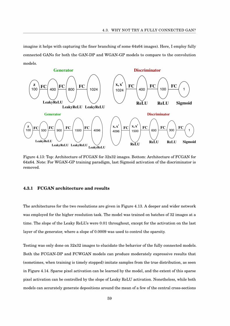
4.3. WHY NOT TRY A FULLY CONNECTED GAN?
imagine it helps with capturing the finer branching of some 64x64 images). Here, I employ fully
connected GANs for both the GAN-DP and WGAN-GP models to compare to the convolution
models.
1024 400 100
400100 1024
1
800
1500 600 300
500100 1500
1
900
4096
4096
Figure 4.13: Top: Architecture of FCGAN for 32x32 images. Bottom: Architecture of FCGAN for
64x64. Note: For WGAN-GP training paradigm, last Sigmoid activation of the discriminator isremoved.
4.3.1 FCGAN architecture and results
The architectures for the two resolutions are given in Figure 4.13. A deeper and wider network
was employed for the higher resolution task. The model was trained on batches of 32 images at a
time. The slope of the Leaky ReLUs were 0.01 throughout, except for the activation on the last
layer of the generator, where a slope of 0.0009 was used to control the sparsity.
Testing was only done on 32x32 images to elucidate the behavior of the fully connected models.
Both the FCGAN-DP and FCWGAN models can produce moderately expressive results that
(sometimes, when training is timely stopped) imitate samples from the true distribution, as seen
in Figure 4.14. Sparse pixel activation can be learned by the model, and the extent of this sparse
pixel activation can be controlled by the slope of Leaky ReLU activation. Nonetheless, while both
models can accurately generate depositions around the mean of a few of the central cross-sections
59

CHAPTER 4. GEANT4 GAN CALORIMETRY MODELING
of the average deposition, their estimates of the standard deviation of these cross-sections was
only intermittently correct. It could not maintain this behavior epoch to epoch once succeeding.
This is seen in Figure 4.18, where in Epoch 82, the FCGAN-DP could not accurately approximate
any of the cross-sectional standard deviations after succeeding to do so, and had strong variation
in its mean estimate outside of the four middle cross sections. As such, training overall was less
stable than in the convolutional case, and each epoch could significantly alter the nature of the
samples produced.
Figure 4.14: Samples from Geant4, GAN-DP, and WGAN-GP models of energy depositions. Modecollapse is evident in the DCGAN-DP samples, where examples in the top right and bottom leftrely on the same modes of the distribution for generation.
60

4.3. WHY NOT TRY A FULLY CONNECTED GAN?
Figure 4.15: Mean and standard deviation of middle cross sections of distribution.
61

CHAPTER 4. GEANT4 GAN CALORIMETRY MODELING
Figure 4.16: Cross-sectional slices through the middle 12 rows of the images.62
MeV
MeV

4.3. WHY NOT TRY A FULLY CONNECTED GAN?
Figure 4.17: Difference between the average 32x32 calorimeter image between Geant4 and boththe FCGAN-DP and FCWGAN paradigms.
63

CHAPTER 4. GEANT4 GAN CALORIMETRY MODELING
Epoch 81
Epoch 82
Figure 4.18: FCGAN-DP cross section metrics in successive epochs. The true standard deviationsare not well approximated by the model in successive epochs
4.3.2 Overall Geant4 GAN discussion
A quick takeaway is that under the right conditions, these GAN models can express diverse
samples from underlying distributions of detector events that are comparable to the true
distribution, with some caveats. There is a trade-off, too, between fully connected and convolutional
models. The DCGAN-DP on the 32x32 resolution detectors and the DCWGAN on the 64x64
detectors train stably (under the right conditions) and produce expressive and diverse samples
that on the average match the true distribution well, but they fail to capture some of the sparser,
64
4.3. WHY NOT TRY A FULLY CONNECTED GAN?
stochastic depositions that one sees in the real events. On the other hand, the fully connected
DCGAN-DP on the 32x32 captures this added sparsity, but fails to train as stably and produces
slightly less expressive samples. It is, above all, a game of making sure they are properly tuned
and that the convolutional architectures are well suited to the data and learning paradigm.
Admittedly, "properly tuned" is a catch-all phrase in machine learning applications, but it is
seemingly more relevant to both GAN models and convolutional methods than other tools and
models. The learning protocols explored here can lead a model to converge in training once, but
not the next time the model is trained from scratch. This was significantly less likely when strong
hyperparameters were found, but not out of the range of possibility.8 These instabilities exist
because GANs circumvent likelihood estimation with this parameterized discriminator/critic.
Because they are in some ways inherent to the model, scaling their use for a wider purview of
simulation might be quite difficult.
Moreover, it’s evident that the learning paradigms don’t necessarily naturally scale equally under
the same convolutional architectures, and that convolution runs the risk of creating unnatural
residual sparsities like the persistent activations in the corner of images from the DCWGAN
32x32 model. The DCGAN-DP model performed slightly better under the 32x32 paradigm using
the same convolutional processes as the DCWGAN, but when these architectures were updated
for 64x64 images, it couldn’t be optimized to overcome the mode collapse seen in Figure 4.12.
There is evidence that some form of them can perform well under some training paradigm on
high resolution data, and the architectures used could be deeper and more nuanced to make
improvements. At higher resolutions, signals are more thinly dispersed through our prototypical
detector. Modern detector technologies would likely take on a higher resolution than even the
ones tested here [47], so it is important to examine if these models can achieve accuracy in sparser
regimes.9
8Moreover, only the WGAN model has a loss function that is better informative of image generation quality, andeven though the gradients of the 1-Lipschitz function approximated by the discriminator can be smoother to traverse,this success is highly dependent on parameter tuning.
9For example, the hadronic end cap in the ATLAS liquid argon calorimeter has a pixel resolution of ¢¥º 0.025and ¢¡º 0.0245. If assuming coverage of 0< |¥| < 2.5, and 0< |¡| <º, images would need to be º 200£256. This couldlikely be partitioned into smaller submodeling tasks, though.
65

CHAPTER 4. GEANT4 GAN CALORIMETRY MODELING
Given the struggle to find a singular GAN framework that captures sparsity and expressiveness
in a stable training paradigm, it is of interest to compare these models to a VAE. It is a model
that is not subject to a parameterized critic and can be trained more stably. This is to see if such
GAN nuances are necessary for building generative models that physicists may use. A more
certain and stable model, if slightly less robust, might appeal more broadly to researchers in
practice.
66
CH
AP
TE
R
5GEANT4 VAE CALORIMETRY
This chapter serves as a comparison to the previous one. It explains some conceptual
differences between GANs and VAEs, as well equivalent Geant4 experiments under
the VAE framework. Its purpose is to weigh the pros and cons of using VAEs to model
calorimetry signals to see what they might offer that GANs do not and where GANs might
outperform them. In it, the efficacy of using Ø-VAEs for conditional generation based on particle
energy is also explored.
5.1 Bring encoding and stability to generation with variational
autoencoders
Just as the excitement around GANs has proliferated over the past few years, so too has the
excitement around variational autoencoding.1 Like GANs, VAEs offer a method of data generation,
but their process for learning this representation and the characteristics of the representation
space differ. Explaining these concepts should be useful for clarifying what benefits or limitations
they bring.1The idea to compare the two came from Dr. David Lopez-Paz, who is currently at Facebook Research.
67

CHAPTER 5. GEANT4 VAE CALORIMETRY
5.1.1 What may VAEs improve or hinder?
To understand the question of what changes VAEs will bring to learning detector images, I will
give a brief comparison of the two models. Recalling from Chapter 1, VAEs encode data into
a lower dimensional space and seek to reconstruct it while adding variation in the encoded
representation to produce new samples. Whereas the GAN takes in an arbitrary noise z and
uses the generator to decode this noise into something in the sample space, the z decoded in a
VAE comes from randomly sampling in a space around where real data has (hopefully) already
been encoded into. One can embed a continuous representation of their data into the latent space
and then make it sample-able by saying that the random samples one generates before decoding
come from some continuous prior p(z). By the end of training, samples of z that one decodes
should continuously cover the space of the original data. This offers a much stabler training
process, where one increases the lower bound of the likelihood of the data by minimizing the
reconstruction error of the decoded samples as well as minimizing the KL-divergence between the
estimated distribution of z and our prior p(z). This may also help with sample diversity, as the
generative samples are not likely to collapse to a few modes if all the samples are encoded into
the latent space. There is no need for a less stable and predictable critic like a neural network to
tell the model how real the samples are – we can get right to the likelihood maximization (or at
least the bounding) and hopefully make more easily reproducible results.
That being said, relying on a reconstruction error and dimensionality reduction can result in
poorer resolution images. Exact values of the true energy deposition or spread might be only
asymptotically approachable due to information loss. This is a known tradeoff between GANs
and VAEs, and I’ll see how they perform in practice.
5.1.2 VAE model architecture
VAEs are composed of an encoder and decoder with a latent space that is used to generate
samples of the latent space z. We can consider the two separate layers that make up this encoding
68

5.1. BRING ENCODING AND STABILITY TO GENERATION WITH VARIATIONALAUTOENCODERS
bottleneck to be a µ mean and a covariance ß used for random sampling. Since we train by
bounding the log-likelihood, we reparameterize to sample from z by saying we actually generate
values of logß and sample during training via:
æ= e12 logß ≤=N ª (0,1) ) z = ≤£æ+µ(5.1)
That’s how the sampling occurs. The dimensionality and structure for both the 32x32 and 64x64
case are given in Figure 5.1. LeakyReLUs were used aside from on the first hidden layer to
encourage the model to capture and produce some of the sparse signals that would otherwise tend
directly toward zero. This can produce a few negative values as energy depositions, which were
cut as non-physical. The same number of layers was kept for both the 32x32 and 64x64, though
the hidden layers were increased in dimensionality as per the figure. Moreover, it was noticed
that making the network any deeper or wider resulted in overfitting and poor generalization on
reconstructing held out test data. Both VAEs were trained on batches of 32 Geant4 events at a
time, with a learning rate of 1£10°4. Models were trained for 300 epochs.2
5.1.3 VAE results
The same metrics and comparisons done for the GAN tests are calculated here as well, again for
32x32 and 64x64 images. This includes comparison of generated samples, the average energy
deposition for distributional comparison, measures of the mean and standard deviation of
the primary central cross sections of the average image, as well as KL-divergence metrics
for distributional comparison.3 The event dataset was split into 25000 training images and 5000
testing to ensure the model did not overfit the data it was trained on. This was done by comparing
loss values between the two sets.
2This was likely unnecessary, as you can see from the plateaued train and test loss in Figure 5.3.3The estimations of the KL-divergence between the average VAE image and average Geant4 image were small
enough that they were strongly influenced by slightly changing the small ≤ = 0.00001 added to the probabilityassociated with each histogram bin during calculation to prevent division by zero. All in all, the distributions werewell matched.
69

CHAPTER 5. GEANT4 VAE CALORIMETRY
1024 750
100
100
300100 1024
300
750
4096 1200
200
200
600200 4096
500
600
Figure 5.1: Top: Architecture of VAE for 32x32 images. Bottom: Architecture of VAE for 64x64. ≤denotes the added noise term for reparameterized sampling.
Table 5.1: KL-divergence estimates between Geant4 average image and VAE average image.
32x32 64x64KL-div 0.0042 0.0089
Table 5.2: Final MSE estimates of reconstruction of Geant4 images by the VAE.
32x32 64x64MSE 40.2 MeV2 46.3 MeV2
Avg event energy dep 200.78 MeV 200.78 MeV
5.1.3.1 32x32 Image results and discussion
The VAE learns a robust approximation of the true distribution and derives samples which
imitate the features seen in real Geant4 samples. One can see that the average images from the
ground truth and the model almost exactly match in Figure 5.2, and that the estimate for the
KL-divergence is almost exactly zero as seen in Table 5.1. Cross sections of this distribution show
precise correspondence, with slight under approximations in the highest values of the two middle
cross-sections with the largest energy depositions as well as in the standard deviations of the
70

5.1. BRING ENCODING AND STABILITY TO GENERATION WITH VARIATIONALAUTOENCODERS
cross-sections throughout. The accuracy of the model monotonically and smoothly improved as
seen in the plot of the losses in Figure 5.3. There is evidence that the model learned embedded
examples of the true examples in Figure 5.5, where one can see how the VAE reconstructed 7
different events. This reconstruction has some limitations in representing some of the finer details
of each collision. The final average MSE loss on the batches was MSE = 40.2 MeV2, where the real
images have average total energy deposition of 200.7 MeV. This approximately 3% reconstruction
error seems to account for the smallest valued pixel activations which generally come at the end
of these branches where a particle finally stopped. Samples of novel generations are provided
in Figure 5.6 which illustrate that the variety of deposition sizes, scales, and characteristic
branching are producible by the VAE while still capturing the sparsely distributed parts of the
event.
The fully connected VAE model, with the right choice of leaky activations as provided here,
learns a comprehensive coverage of the true Geant4 distribution of 32x32 images with expressive
samples. One caveat of this method, though, is the reliance on data reconstruction. The plateaued
loss function and slightly underestimated peak values of energy depositions seen in Figure 5.3
and 5.4 are byproducts of this. The VAE will asymptotically approach these true values but is
limited by reconstruction based on dimensionality reduction, much like creating a blurry photo
by extracting the important features of the original image. It captures the important aspects of
the space, but isn’t perfectly clear. While GANs may collapse to restricted modes of the data, they
generally create clearer images that are not bound by asymptotic learning. One can see in Figure
4.5 that the GAN can overestimate and underestimate these same cross-sectional peaks that
the VAE may only approach, suggesting some of the greater flexibility in what the GAN has the
potential to learn. This is further elucidated in Figure 5.7, where one can see that the VAE can
only approach the mean pixel energy deposition, while the DCWGAN can reach and move down
from it.
71

CHAPTER 5. GEANT4 VAE CALORIMETRY
Figure 5.2: Comparison of Average VAE image to average Geant4 image at 32x32 resolution.
72

5.1. BRING ENCODING AND STABILITY TO GENERATION WITH VARIATIONALAUTOENCODERS
Figure 5.3: Analysis of features of the average VAE detector image at 32x32 resolution. Top:Difference between the average images of Geant4 and the VAE; train and test loss across epochs.Bottom: Mean and and standard deviation of these 1D cross sectional histograms
73

CHAPTER 5. GEANT4 VAE CALORIMETRY
Figure 5.4: Comparison of central cross-sections of average image.
74
MeV

5.1. BRING ENCODING AND STABILITY TO GENERATION WITH VARIATIONALAUTOENCODERS
Figu
re5.
5:R
econ
stru
ctio
nof
6ev
ents
byVA
E
75

CHAPTER 5. GEANT4 VAE CALORIMETRY
Figure 5.6: VAE and Geant4 samples of 32x32 images.
Figure 5.7: Comparing average pixel energy deposition between DCWGAN and VAE models.
76

5.1. BRING ENCODING AND STABILITY TO GENERATION WITH VARIATIONALAUTOENCODERS
5.1.3.2 64x64 Image results and discussion
Equivalent training and analysis was done for the 64x64 resolution images. An approximate
estimation of the true distribution was attained like in the 32x32 case, but again with an
underestimation of the standard deviations of the cross-sections and some variation on the
cross-sectional mean estimates. These standard deviation underestimations were slightly worse
for cross-sections farther from the centroid, as seen in the bottom of Figure 5.9. After 300 epochs
the average image for both are nearly identical, and the difference of the two is near zero
throughout, with slight underestimation on center pixels of the middle cross-sections like in the
lower resolution case. The KL-divergence seen in Table 5.1, while slightly greater than in the
32x32 case, is still near zero.
The model reconstructs the samples of real data with some expressiveness in the branching of
depositions and uses this information to create new depositions that are both sparse and diverse.
That being said, some of the finer details of the reconstruction are not captured, as would be
suggested by the nonzero loss plateau seen at the top of Figure 5.9 and in the reconstructions
seen in Figure 5.11. The final average MSE loss on the batches was MSE = 46.3 MeV2, where
the real images have average total energy deposition of 200.7 MeV, which implies approximately
a 3.5% difference between the real and decoded samples. This reconstruction limit is likely the
reason why some of the most extensive branching that is seen in the figure of reconstructions and
the real samples of Figure 5.12 is not fully captured by the VAE. The energy that would have been
combined into one pixel bin in the 32x32 case is now spread across more, lowering the activation
in each and making it less likely to be represented in the lower dimensional latent space. A
deeper network with more non-linear activations, or wider layers and bottleneck, might help
circumvent this. The data was slightly overtrained on the training set, as per the loss in Figure
5.9, though training could have stopped earlier before such at the beginning of the reconstruction
plateau around epoch 75.
While the scaling of the VAE to 64x64 exacerbated some of the limitations of the 32x32 model,
the model still learns a continuous and comprehensive approximation of the underlying ground
77

CHAPTER 5. GEANT4 VAE CALORIMETRY
truth, and does so in an easily trainable way. The difference between the average image of the
VAE and Geant4 compared to its fully connected GAN connected GAN counterpart as well its
successful minimization of the KL-divergence of the model and target distribution suggest that it
still learns to accurately imitate real simulation, and this is decently evident in the samples.
Figure 5.8: Comparison of average images of VAE on 64x64 resolution events.
78

5.1. BRING ENCODING AND STABILITY TO GENERATION WITH VARIATIONALAUTOENCODERS
Figure 5.9: Analysis of features of the average VAE detector image at 64x64 resolution. Top:Difference between the average images of Geant4 and the VAE; train and test loss across epochs.Bottom: Mean and and standard deviation of these 1D cross sectional histograms
79

CHAPTER 5. GEANT4 VAE CALORIMETRY
Figure 5.10: Middle: Comparison of central cross-sections of average image.
80
MeV

5.1. BRING ENCODING AND STABILITY TO GENERATION WITH VARIATIONALAUTOENCODERS
Figu
re5.
11:R
econ
stru
ctio
nof
6ev
ents
byVA
Eat
64x6
4
81

CHAPTER 5. GEANT4 VAE CALORIMETRY
Figure 5.12: VAE and Geant4 samples of 64x64 images.
5.1.4 Conditional generation with VAEs
Given the capability of learning event representations with the fully connected VAE models, it is
of interest to show that it too, like the GAN, can take in conditional physics information to inform
event generation. By supplying information about the energy of the incoming particle at the
encoding and decoding stages of the VAE’s learning paradigm, the model can learn to make use of
this auxiliary input to inform its behavior. The goal, like in the previous conditional generations
produced in Chapters 2 and 3, is to ensure that the conditions are correlated to events with
82

5.1. BRING ENCODING AND STABILITY TO GENERATION WITH VARIATIONALAUTOENCODERS
the right corresponding output characteristics. That is, the when a certain energy condition is
supplied, the model should only generate calorimeter images that fall under the domain of that
conditional distribution.
5.1.4.1 Conditional VAE architecture and training
A Conditional VAE (CVAE) for 32x32 images was constructed of equivalent architecture as that
seen in Section 5.1.3.1, with the addition of energy information supplied at the first encoding and
decoding layers. The model was trained on images that arose from 3 electron gun energies: 100
MeV, 800 MeV, and 1800 MeV. The events were shuffled such that each (image, energy) pair were
given in a random batch of 32 images at time. Energies were normalized so as to not introduce
the bias of outlying large values.
5.1.4.2 Ø-VAEs to improve conditionality and trade-off
To enforce greater pressure on the independence of the latent space as well as to make the model
learn the most efficient representation of the data, I introduce a Ø-CVAE learning paradigm at
this point in the experimentation. Ø-VAEs are a recent modification introduced to the original
VAE model which puts a regularizing coefficient Ø > 1 on the KL-divergence of the inference
encoding of the data q¡(z|x) and our chosen Gaussian prior p(z) [48]. The lower bound can then
be described as:
(5.2) ln p(x)∏ Ezªq¡(z|x)[ln pµ(x|z)]°ØDKL(q¡(z|x) || pµ(z))
The purpose of such coefficient is to put greater pressure on the latent space to adopt the qualities
of this isotropic Gaussian, which would help encourage conditional independence in q¡(z|x).
When additional conditional information is included in the model, I surmise the greater pressure
on creating a bottleneck with conditional independence should help the VAE model properly
make use of the auxiliary information.
83
CHAPTER 5. GEANT4 VAE CALORIMETRY
One limitation of this tuning is that the reconstruction error is given less import in the loss and
as such the latent space has less capacity to embed finer details needed for the reconstruction
and generation of old and new data, respectively. This can result in a bit of a game of tuning the
parameters between generative capacity and adoption of conditional information. 4
5.1.4.3 Ø-CVAE architecture and results
Ø-CVAE models with network architecture equivalent to the training regime in Section 5.1.3.1
other than the addition of the conditional information at the 1st encoding and decoding layers
were tested with a variety of Ø values: 1, 2.5, 4, 8. Batch sizes and learning rates were also
equivalent to the unconditional 32x32 VAE modeling. The results of capturing the conditional
information are seen in Figure 5.13 where the mean value of the deposition depending on
condition is plotted for the Geant4 events compared to the fake events. The means for 500 events
are distributed in light matching colors over each energy condition to show spread. This is done
for each of the four Ø values. One can see that there is not much improvement on the mean
estimate for each energy beyond using a Ø value of 2.50. The fact that the means fall short is
in line with the results of the unconditional VAE, for which it was noted that the VAE tries to
approach the true mean deposition, but plateaus and underestimates it. Moreover, one can see
that the sample quality diminishes as the Ø value is increased in Figure 5.14. The sample quality
for the Ø = 2.5 case is not significantly diminished, but the quality falls off for Ø∏ 4
4Work in [49] recently suggests that the KL-divergence term can be broken down into 3 subcomponents, one ofwhich called the total correlation is primarily responsible for driving this adoption of conditional independence. Thetotal correlation is really in some ways a direct measure of component-wise independence. It is the a measure of theKL-divergence between the joint latent distribution and the product of its marginals: TC= DKL(q(z)||Qi q(zi))
84

5.1. BRING ENCODING AND STABILITY TO GENERATION WITH VARIATIONALAUTOENCODERS
Figure 5.13: The mean energy deposition for Geant4 vs. Ø-CVAE data conditioned on particleenergy for 4 different Ø values.
85
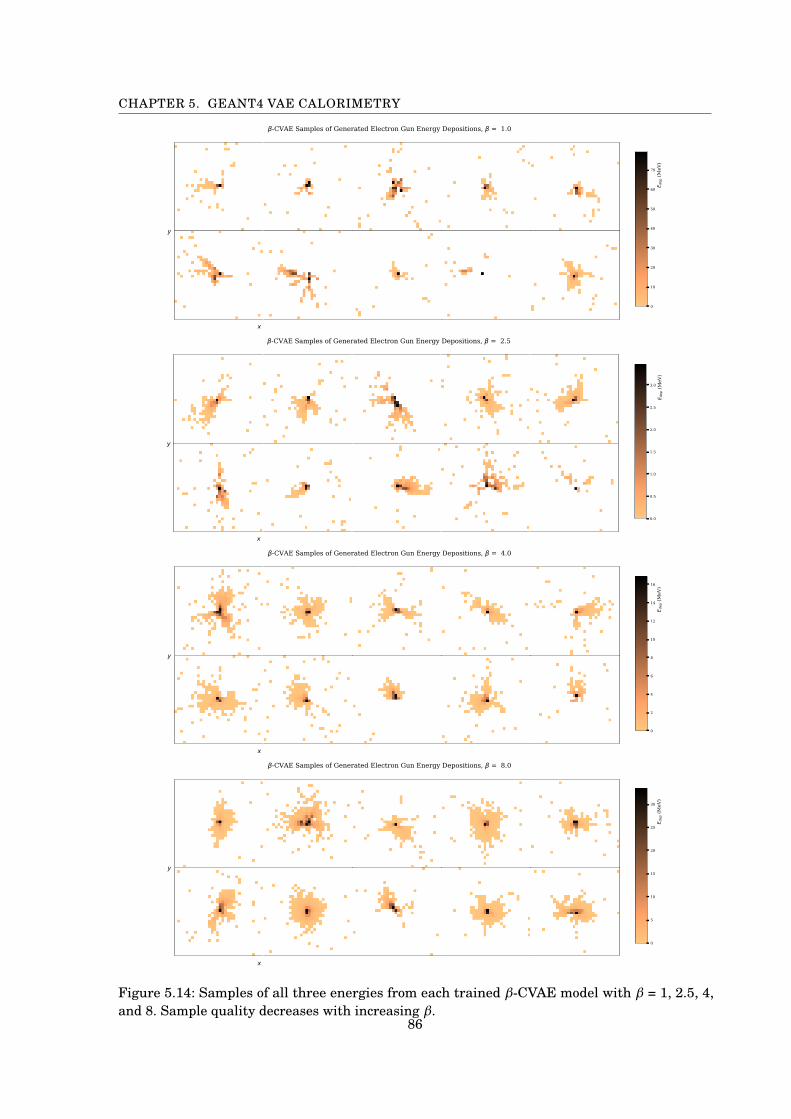
CHAPTER 5. GEANT4 VAE CALORIMETRY
Figure 5.14: Samples of all three energies from each trained Ø-CVAE model with Ø = 1, 2.5, 4,and 8. Sample quality decreases with increasing Ø.
86

CH
AP
TE
R
6CONCLUSION
This has been a brief journey through exploring recent generative models and their
applications to particle physics detector simulation. The goal has been to build from
the ground up, with an original focus just on GANs. The model and its varied training
paradigms were built and tested on toy datasets to perform some analysis of which methods might
be the most robust to proceed with. We saw that the GAN-DP model could efficiently and stably
model the toy datasets, and that the WGAN-GP could under a training regimen with very small
gradient updates. We also saw that the GAN could make conditional generations, and extrapolate
to conditions beyond just those that it trained on. From there, these techniques were introduced
to a physics landscape, and it was shown that aspects of simple detector simulators like PT
mis-measurement can be replicated under GAN training protocols, including data generation
based on conditional physics information with varying scales of influence on such generation.
Most importantly, this built up to modeling simulations that are complex and computationally
expensive enough to warrant an alternative method, something that has already recently been
explored in the particle physics community [35, 36]. The purpose of such was i) to validate these
recent results ii) to explore how different variations of GAN architectures and training paradigms
deal with the unique character of these sparse distributions iii) to test the models in higher
87

CHAPTER 6. CONCLUSION
resolution settings to see the limits of the model complexity. After analyzing the way convolutional
GANs and fully connected GANs both had their promising aspects and negative traits, VAEs were
introduced to complete the same task for comparison. The deep convolutional GAN, under the
right sensitive training conditions, offered expressive samples that modeled the true distribution,
but fell short on the sparser aspects of the signals. Moreover, its training paradigms had variable
success on the different image resolutions. The fully connected GAN suffered from even greater
training instabilities, but captured the sparser signals when it worked. The VAE provided a
stabler training regime that captured this sparsity and consistently learned an imitation of the
sample distribution regardless of detector resolution, but can be limited in sample quality at
higher resolutions by its reliance on reconstruction loss. In a way, it provided the best of both
worlds from the two GAN setups. I also introduced a Ø-CVAE for detector simulation that can
improve the adoption of conditional physics information by the model, such as particle energy.
Above all, the question remains what speedup these models would present to their Geant4
counterpart. The times it took to produce a single 800 MeV event for the set of ML models and
Geant4 are given in Table 6.1.1 The fully connected models both train faster and produce events
faster, producing at most 1000 times as fast as Geant4. This was of course, on a GPU, and there is
likely a way for me to implement the Geant4 method faster, but a speedup is evident nonetheless.
Moreover, it takes time to train a model, so depending on how versatile and useful your model
is in the long term, that may or may not be taken into account. The DCGAN also saw orders of
magnitude speedup. It is here that the potential of these models really becomes apparent.
6.1 Future improvements
While both the GANs and VAEs show high potential for being incorporated into the particle
physics simulation repertoire, there are many avenues for improvement. GANs are consistently
being improved year to year, either through new conceptualizations or training criteria that work
1ML models were calculated on single Nvidia Titan XP GPU while Geant4 was on CPU. Geant4 modeling timescaled with particle energy.
88

6.1. FUTURE IMPROVEMENTS
toward stability and convergence such as the recently proposed Coulomb GAN [50].2 One way to
directly approach uniting sparse signals with convolution would be to use sparse convolutional
networks like those of [51] that are designed to function with this type of data. VAEs are subject
to the same spirit of innovation, and recent improvements to them could help with sample quality.
One could replace the VAE with a Wasserstein Autoencoder [52] or combine some of the benefits
of adversarial training with some of the benefits of VAEs using Adversarial Autoencoders [53, 54].
The latent space to which data is encoded can be given more thoughtful consideration as well. To
get the CVAE to better use the conditional information, one could implement the improvements
to the Ø-VAE discussed in [49] and [55] by focusing on penalizing the total correlation rather than
the entire KL-divergence between the encoded inference distribution and the Gaussian prior. One
could also make a smarter choice of prior that aligns better to the space the data is distributed
in. For example, if your data has a certain topology you would like to preserve, SO(3)-valued
latent variables can be chosen to better preserve this and capture rotation in the latent space [56].
Lastly, greater consideration could be given to figuring out how to scale up these example tests so
that they could be efficient and versatile enough to be adopted by the research community. This
could mean standardizing the way new models are trained or choosing the best set of conditional
information a model learns to give it the most breadth and versatility. The reproducibility and
trustability of VAEs is one reason they might be more appealing to researchers in the short term.
Above all, generative models offer a new frontier of data representation and manipulation. They
are a set of tools that physicists can and already have taken advantage of. GANs and VAEs are
two of such methods that, herein, showed the potential for future use in the world of particle
physics simulation. Hopefully, that potential will be fulfilled by continued improvement to their
theory and implementation.
2This is a personal favorite because it is inspired by electromagnetic potentials.
89

Table 6.1: Time to produce single e° gun image in seconds.
Model 32x32 64x64FCVAE (GPU) 0.000751 s 0.00103 sFCGAN (GPU) 0.000663 s 0.00168 sDCGAN (GPU) 0.00150 s 0.00248 sFCVAE (CPU) 0.0122 s 0.0305 sFCGAN (CPU) 0.0108 s 0.0322 sDCGAN (CPU) 0.0233 s 0.0497 sGeant4 - 800 MeV 0.791 s 0.798 s

AP
PE
ND
IX
AAPPENDIX A
Aspace for definitions and further details.
A.1 Chapter 1 Notes
Kullback-Leibler Divergence: KL-Divergence is an ubiquitous metric for comparing the
similarity between a probability distribution and a target probability distribution. It is commonly
used for comparing inference models. It is defined as
DKL(P||Q)=°X
iP(xi) ln
P(xi)Q(xi)
It is not a distance metric because it is not symmetric. It can be better thought of as a measure of
entropy increase due to using approximate distribution rather than the true distribution. Q is
that approximate distribution. It is minimized when the probabilities are aligned.
91
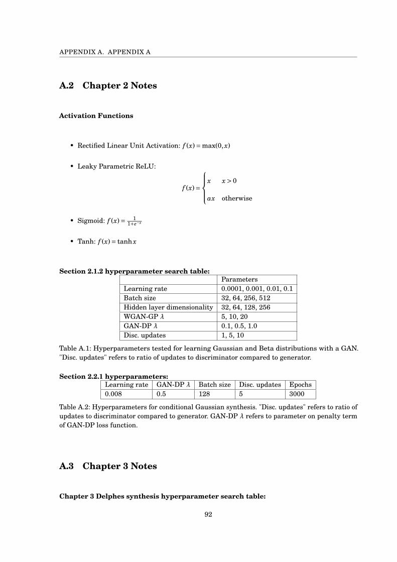
APPENDIX A. APPENDIX A
A.2 Chapter 2 Notes
Activation Functions
• Rectified Linear Unit Activation: f (x)=max(0, x)
• Leaky Parametric ReLU:
f (x)=
8>><
>>:
x x > 0
ax otherwise
• Sigmoid: f (x)= 11+e°x
• Tanh: f (x)= tanh x
Section 2.1.2 hyperparameter search table:Parameters
Learning rate 0.0001, 0.001, 0.01, 0.1Batch size 32, 64, 256, 512Hidden layer dimensionality 32, 64, 128, 256WGAN-GP ∏ 5, 10, 20GAN-DP ∏ 0.1, 0.5, 1.0Disc. updates 1, 5, 10
Table A.1: Hyperparameters tested for learning Gaussian and Beta distributions with a GAN."Disc. updates" refers to ratio of updates to discriminator compared to generator.
Section 2.2.1 hyperparameters:Learning rate GAN-DP ∏ Batch size Disc. updates Epochs0.008 0.5 128 5 3000
Table A.2: Hyperparameters for conditional Gaussian synthesis. "Disc. updates" refers to ratio ofupdates to discriminator compared to generator. GAN-DP ∏ refers to parameter on penalty termof GAN-DP loss function.
A.3 Chapter 3 Notes
Chapter 3 Delphes synthesis hyperparameter search table:
92

A.4. CHAPTER 4 NOTES
ParametersLearning rate 0.0001, 0.001, 0.01, 0.1Batch size 32, 64, 256, 512Hidden layer dimensionality 32, 64, 128, 256GAN-DP ∏ 0.1, 0.5, 1.0Disc. updates 1, 5, 10
Table A.3: Hyperparameters tested for conditional Delphes PT smearing. "Disc. updates" refersto ratio of updates to discriminator compared to generator.
A.4 Chapter 4 Notes
Standard EM physics used by Geant4 in QGSP-BERT:
• multiple scattering, electron ionization, electron bremsstrahlung, e+e- annihilation, e+e-
annihilation to hadrons, e+e- annihilation to mu pair, muon ionization, muon bremsstrahlung,
e+e- pair production by muons, hadron ionization, ion ionization, Compton scattering,
polarized Compton scattering, photo-electric effect, gamma conversion, gamma conversion
to muons, Cerenkov radiation, scintillation, synchrotron radiation, forward transition
radiation, transition radiation, gamma, transition radiation, regular, transition radiation,
straw tube, transition radiation, transparent
93


AP
PE
ND
IX
BAPPENDIX B
Aspace for backup plots that may be unnecessary for argumentation in the full document,
but could still be supporting.
B.1 Chapter 1 Notes
Finding WGAN-GP Beta Generation stability: WGAN-GP training on the toy dataset shows
instability at learning rates > 0.00001. Local convergence only found once reaching 0.00001:
• Learning rate 0.001:
• Learning rate 0.0001:
95

APPENDIX B. APPENDIX B
• Learning rate 0.00001:
• Local convergence only found with smallest gradient steps.
96

BIBLIOGRAPHY
[1] Y. Lecun, Y. Bengio, and G. Hinton, “Deep learning,” Nature, vol. 521, no. 7553, pp. 436–444,
2015.
[2] A. Owen, “Monte Carlo theory, methods and examples,” vol. 2, pp. 1–19, 2013.
[3] C. Andrieu, N. De Freitas, A. Doucet, and M. I. Jordan, “An introduction to MCMC for
machine learning,” Machine Learning, vol. 50, no. 1-2, pp. 5–43, 2003.
[4] T. Sjöstrand, S. Mrenna, and P. Skands, “A brief introduction to PYTHIA 8.1,” Computer
Physics Communications, vol. 178, no. 11, pp. 852–867, 2008.
[5] J. de Favereau, C. Delaere, P. Demin, A. Giammanco, V. Lemaitre, A. Mertens, and
M. Selvaggi, “DELPHES 3: A modular framework for fast-simulation of generic collider
experiments,” Journal of Physics: Conference Series, vol. 523, no. 1, 2014.
[6] S. Agostinelli, “GEANT4 - A simulation toolkit,” Nuclear Instruments and Methods in Physics
Research, Section A: Accelerators, Spectrometers, Detectors and Associated Equipment,
vol. 506, no. 3, pp. 250–303, 2003.
[7] M. G. Pia, T. Basaglia, Z. W. Bell, and P. V. Dressendorfer, “Geant4 in scientific literature,”
IEEE Nuclear Science Symposium Conference Record, pp. 189–194, 2009.
[8] L. D. Oliveira, M. Kagan, L. Mackey, and B. Nachman, “Jet-Images – Deep Learning Edition,”
Journal of High Energy Physics, vol. 2, no. 118, 2015.
[9] P. Domingos, “A few useful things to know about machine learning,” Communications of the
ACM, vol. 55, no. 10, p. 78, 2012.
97

BIBLIOGRAPHY
[10] I. Goodfellow, “NIPS 2016 Tutorial: Generative Adversarial Networks,” in Neural
Information Processing Systems, 2016.
[11] L. Theis, A. v. d. Oord, and M. Bethge, “A note on the evaluation of generative models.” 2016.
[12] I. J. Goodfellow, J. Pouget-Abadie, M. Mirza, B. Xu, D. Warde-Farley, S. Ozair, A. Courville,
and Y. Bengio, “Generative Adversarial Networks,” in Neural Information Processing
Systems, 2014.
[13] K. Roth, A. Lucchi, S. Nowozin, and T. Hofmann, “Stabilizing Training of Generative
Adversarial Networks through Regularization,” in Neural Information Processing
Systems, pp. 1–16, 2017.
[14] M. Arjovsky, S. Chintala, and L. Bottou, “Wasserstein GAN,” in International Conference
Machine Learning, 2017.
[15] T. Che, Y. Li, A. P. Jacob, Y. Bengio, and W. Li, “Mode Regularized Generative Adversarial
Networks,” in ICLR, pp. 1–13, 2017.
[16] I. Gulrajani, F. Ahmed, M. Arjovsky, V. Dumoulin, and A. Courville, “Improved Training of
Wasserstein GANs,” in Neural Information Processing Systems, pp. 1–19, 2017.
[17] M. Arjovsky and L. Bottou, “Towards Principled Methods for Training Generative
Adversarial Networks,” in ICLR, pp. 1–17, 2017.
[18] L. Mescheder, A. Geiger, and S. Nowozin, “Which Training Methods for GANs do actually
Converge?,” in International Conference on Learning Representations (ICLR), 2018.
[19] D. Rumelhart, G. Hinton, and R. Williams, “Learning Internal Representations by Error
Propagation,” in Parallel distributed processing: explorations in the microstructure of
cognition, vol. 1, pp. 318–362, 1985.
[20] P. Vincent and H. Larochelle, “Stacked Denoising Autoencoders: Learning Useful
Representations in a Deep Network with a Local Denoising Criterion Pierre-Antoine
Manzagol,” Journal of Machine Learning Research, vol. 11, pp. 3371–3408, 2010.
98

BIBLIOGRAPHY
[21] A. Ng, “Lecture Notes Sparse Autoencoder,” in Stanford CS294A Lecture notes, pp. 1–19,
2011.
[22] S. Rifai and X. Muller, “Contractive Auto-Encoders : Explicit Invariance During Feature
Extraction,” International Conference Machine Learning, vol. 85, no. 1, pp. 833–840,
2011.
[23] D. P. Kingma and M. Welling, “Auto-Encoding Variational Bayes,” in International
Conference on Learning Representations, 2014.
[24] C. Doersch, “Tutorial on Variational Autoencoders,” tech. rep., 2016.
[25] F.-F. Li, J. Johnson, and S. Yeung, “Lecture Notes on Generative Models,” in Stanford CS231n
Lecture notes, 2017.
[26] C. P. Burgess, I. Higgins, A. Pal, L. Matthey, N. Watters, G. Desjardins, and A. Lerchner,
“Understanding disentangling in Beta-VAE,” in Neural Information Processing Systems,
2018.
[27] B. Denby, “Neural networks and cellular automata in experimental high energy physics,”
Computer Physics Communications, vol. 49, no. 3, pp. 429–448, 1988.
[28] J. Brehmer, K. Cranmer, G. Louppe, and J. Pavez, “Constraining Effective Field Theories
with Machine Learning,” Physical Review Letters, vol. 121, no. 111801, pp. 1–5, 2018.
[29] S. Caron, J. S. Kim, K. Rolbiecki, R. R. de Austri, and B. Stienen, “The BSM-AI project:
SUSY-AI–generalizing LHC limits on supersymmetry with machine learning,” European
Physical Journal C, vol. 77, no. 4, 2017.
[30] CMS Collaboration, “Identification of heavy-flavour jets with the CMS detector in pp
collisions at 13 TeV,” 2017.
[31] B. Nachman, M. Paganini, and L. de Oliveira, “Survey of Machine Learning Techniques for
High Energy Electromagnetic Shower Classification,” no. Dlps, pp. 1–6, 2017.
99

BIBLIOGRAPHY
[32] E. M. Metodiev, B. Nachman, and J. Thaler, “Classification without labels: learning from
mixed samples in high energy physics,” Journal of High Energy Physics, vol. 2017, no. 10,
2017.
[33] V. V. Gligorov and M. Williams, “Efficient, reliable and fast high-level triggering using a
bonsai boosted decision tree,” Journal of Instrumentation, vol. 8, no. 2, 2013.
[34] P. Baldi, P. Sadowski, and D. Whiteson, “Searching for exotic particles in high-energy physics
with deep learning,” Nature Communications, vol. 5, pp. 1–14, 2014.
[35] L. de Oliveira, M. Paganini, and B. Nachman, “Learning Particle Physics by Example:
Location-Aware Generative Adversarial Networks for Physics Synthesis,” Computing
and Software for Big Science, vol. 1, no. 4, 2017.
[36] M. Paganini, L. de Oliveira, and B. Nachman, “CaloGAN: Simulating 3D High Energy
Particle Showers in Multi-Layer Electromagnetic Calorimeters with Generative
Adversarial Networks,” Physical Review D, vol. 97, no. 014021, 2018.
[37] J. Cogan, M. Kagan, E. Strauss, and A. Schwartzman, “Jet-Images: Computer Vision Inspired
Techniques for Jet Tagging,” 2014.
[38] P. T. Komiske, E. M. Metodiev, and M. D. Schwartz, “Deep learning in color: towards
automated quark/gluon jet discrimination,” Journal of High Energy Physics, vol. 2017,
no. 1, 2017.
[39] G. Louppe, K. Cho, C. Becot, and K. Cranmer, “QCD-Aware Recursive Neural Networks for
Jet Physics,” ArXiv Preprint., pp. 1–11, 2018.
[40] D. P. Kingma and J. L. Ba, “Adam: A Method for Stochastic Optimization,” in International
Conference on Learning Representations (ICLR), 2015.
[41] M. Mirza and S. Osindero, “Conditional Generative Adversarial Nets,” ArXiv Preprint.,
pp. 1–7.
[42] S. Ovyn and X. Rouby, “Delphes, a framework for fast simulation of a generic collider
experiment,” ArXiv Preprint., p. 36, 2009.
100
BIBLIOGRAPHY
[43] K. Fukushima, “Neocognitron: A hierarchical neural network capable of visual pattern
recognition,” Neural Networks, vol. 1, no. 2, pp. 119–130, 1988.
[44] A. Krizhevsky, I. Sutskever, and G. E. Hinton, “ImageNet Classification with Deep
Convolutional Neural Networks,” Advances In Neural Information Processing Systems,
pp. 1–9, 2012.
[45] D. Guest, K. Cranmer, and D. Whiteson, “Deep Learning and its Application to LHC Physics,”
Annual Review of Nuclear and Particle Science, vol. 68, pp. 1–22, 2018.
[46] A. Radford, L. Metz, and S. Chintala, “Unsupervised Representation learning with Deep
Convolutional GANs,” International Conference on Learning Representations, pp. 1–16,
2016.
[47] H. Wilkens, “The ATLAS liquid argon calorimeter: An overview,” Journal of Physics:
Conference Series, vol. 160, 2009.
[48] I. Higgins, L. Matthey, A. Pal, C. Burgess, X. Glorot, M. Botvinick, S. Mohamed, and
A. Lerchner, “B-Vae: Learning Basic Visual Concepts With a Constrained Variational
Framework,” International Conference on Learning Representations, no. July, pp. 1–13,
2017.
[49] T. Q. Chen, X. Li, R. Grosse, and D. Duvenaud, “Isolating Sources of Disentanglement in
Variational Autoencoders,” International Conference on Learning Representations, 2018.
[50] T. Unterthiner, B. Nessler, C. Seward, G. Klambauer, M. Heusel, H. Ramsauer, and
S. Hochreiter, “Coulomb GANs: Provably Optimal Nash Equilibria via Potential Fields,”
International Conference on Learning Representations, pp. 1–21, 2018.
[51] B. Graham, “Spatially-sparse convolutional neural networks,” ArXiv Preprint., pp. 1–13,
2014.
[52] I. Tolstikhin, S. Gelly, O. Bousquet, C.-J. Simon-Gabriel, and B. Schölkopf, “AdaGAN:
Boosting Generative Models,” Neural Information Processing Systems, pp. 1–31, 2017.
101

BIBLIOGRAPHY
[53] A. Makhzani, J. Shlens, N. Jaitly, I. Goodfellow, and B. Frey, “Adversarial Autoencoders,”
International Conference on Learning Representations, 2016.
[54] L. Mescheder, S. Nowozin, and A. Geiger, “Adversarial Variational Bayes: Unifying
Variational Autoencoders and Generative Adversarial Networks,” in International
Conference Machine Learning, 2017.
[55] H. Kim and A. Mnih, “Disentangling by Factorising,” International Conference Machine
Learning, 2018.
[56] L. Falorsi, P. de Haan, T. R. Davidson, N. De Cao, M. Weiler, P. Forré, and T. S. Cohen,
“Explorations in Homeomorphic Variational Auto-Encoding,” in International Conference
Machine Learning, 2018.
102
Related Documents