Toward an optimal geomagnetic field intensity determination technique

Toward an optimal geomagnetic field intensity determinationtechnique

Yongjae Yu, Lisa Tauxe, and Agnes GeneveyScripps Institution of Oceanography, La Jolla, California 92093, USA ([email protected]; [email protected];[email protected])

[1] Paleointensity determinations based on double heating techniques (in-field/zero-field cooling, zero-

field/in-field cooling, and two in-field steps with opposite laboratory fields) are generally considered to be

functionally interchangeable producing equally reliable paleointensity estimates. To investigate this

premise, we have developed a simple mathematical model. We find that both the zero-field first and in-

field first methods have a strong angular dependence on the laboratory field (parallel, orthogonal, and anti-

parallel) while the two in-field steps method is independent of the direction of the laboratory-produced

field. Contrary to common practice, each method yields quite different outcomes if the condition of

reciprocity of blocking and unblocking temperatures is not met, even with marginal (10%) tails of partial

thermoremanence. Our calculations suggest that the zero field first method with the laboratory-produced

field anti-parallel to the natural remanence (NRM) is the most robust paleointensity determination

technique when the intensity of the lab-induced field is smaller than ancient field. However, the zero field

first method with the laboratory-field parallel to the NRM is the optimum approach when the intensity of

the lab-induced field is larger than the ancient field. By far the best approach, however, is to alternatethe

infield-zerofield (IZ) steps with zerofield-infield (ZI) steps.

Components: 6969 words, 7 figures, 2 tables.

Keywords: Paleointensity; TRM; pTRM; pTRM Tail; Theillier.

Index Terms: 1521 Geomagnetism and Paleomagnetism: Paleointensity; 1594 Geomagnetism and Paleomagnetism:

Instruments and techniques; 1500 Geomagnetism and Paleomagnetism.

Received 8 September 2003; Revised 17 December 2003; Accepted 26 December 2003; Published 26 February 2004.

Yu, Y., L. Tauxe, and A. Genevey (2004), Toward an optimal geomagnetic field intensity determination technique, Geochem.

Geophys. Geosyst., 5, Q02H07, doi:10.1029/2003GC000630.

————————————

Theme: Geomagnetic Field Behavior Over the Past 5 Myr Guest Editors: Cathy Constable and Catherine Johnson

1. Introduction

[2] The geomagnetic field is one of the most

intriguing features of the Earth. The Earth’s mag-

netic field originates in the liquid outer core, as a

result of electric currents generated by a self-

sustaining dynamo. The geomagnetic field is a

vector quantity, so that both direction and intensity

are required to describe it at any position on the

Earth’s surface. It is far from being constant either

in magnitude or in direction and varies spatially as

well as in time. Compared to directional studies,

there are far fewer studies on the intensity varia-

tions of the geomagnetic field. Geomagnetic field

intensity variations are of particular importance

because of their direct relevance to the geodynamo,

G3G3GeochemistryGeophysics

Geosystems

Published by AGU and the Geochemical Society

AN ELECTRONIC JOURNAL OF THE EARTH SCIENCES

GeochemistryGeophysics

Geosystems

Article

Volume 5, Number 2

26 February 2004

Q02H07, doi:10.1029/2003GC000630

ISSN: 1525-2027

Copyright 2004 by the American Geophysical Union 1 of 18

growth of the inner core, and evolution of core-

mantle boundary.

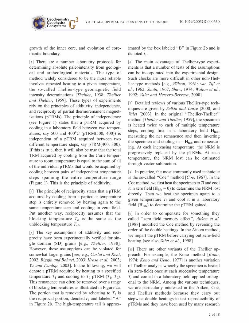
[3] There are a number laboratory protocols for

determining absolute paleointensity from geologi-

cal and archeological materials. The type of

method widely considered to be the most reliable

involves repeated heating to a given temperature,

the so-called Thellier-type geomagnetic field

intensity determinations [Thellier, 1938; Thellier

and Thellier, 1959]. These types of experiments

rely on the principles of additivity, independence,

and reciprocity of partial thermoremanent magnet-

izations (pTRMs). The principle of independence

(see Figure 1) states that a pTRM acquired by

cooling in a laboratory field between two temper-

atures, say 500 and 400�C (pTRM(500, 400)) is

independent of a pTRM acquired between two

different temperature steps, say pTRM(400, 300).

If this is true, then it will also be true that the total

TRM acquired by cooling from the Curie temper-

ature to room temperature is equal to the sum of all

of the individual pTRMs that would be acquired by

cooling between pairs of independent temperature

steps spanning the entire temperature range

(Figure 1). This is the principle of additivity.

[4] The principle of reciprocity states that a pTRM

acquired by cooling from a particular temperature

step is entirely removed by heating again to the

same temperature step and cooling in zero field.

Put another way, reciprocity assumes that the

blocking temperature Tb is the same as the

unblocking temperature Tub.

[5] The key assumptions of additivity and reci-

procity have been experimentally verified for sin-

gle domain (SD) grains [e.g., Thellier, 1938].

However, these assumptions can be violated for

somewhat larger grains [see, e.g., Carlut and Kent,

2002; Biggin and Bohnel, 2003; Krasa et al., 2003;

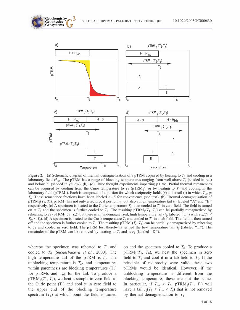
Yu and Dunlop, 2003]. In the following, we will

denote a pTRM acquired by heating to a specified

temperature T1 and cooling to T0 pTRM"(T1, T0).

This remanence can often be removed over a range

of blocking temperatures as illustrated in Figure 2a.

The portion that is removed by reheating to T1 is

the reciprocal portion, denoted r" and labeled ‘‘A’’

in Figure 2b. The high-temperature tail is approx-

imated by the box labeled ‘‘B’’ in Figure 2b and is

denoted t".

[6] The main advantage of Thellier-type experi-

ments is that a number of tests of the assumptions

can be incorporated into the experimental design.

Such checks are more difficult in other non-Thel-

lier-type methods [e.g., Wilson, 1961; van Zijl et

al., 1962; Smith, 1967; Shaw, 1974; Walton et al.,

1992; Valet and Herrero-Bervera, 2000].

[7] Detailed reviews of various Thellier-type tech-

niques are given by Selkin and Tauxe [2000] and

Valet [2003]. In the original ‘‘Thellier-Thellier’’

method [Thellier and Thellier, 1959], the specimen

is heated twice to each of multiple temperature

steps, cooling first in a laboratory field Hlab,

measuring the net remanence and then inverting

the specimen and cooling in �Hlab and remeasur-

ing. At each increasing temperature, the NRM is

progressively replaced by the pTRMs. At each

temperature, the NRM lost can be estimated

through vector subtraction.

[8] In practice, the most commonly used technique

is the so-called ‘‘Coe’’ method [Coe, 1967]. In the

Coemethod,we first heat the specimen toTi and cool

it in zero field (Hlab = 0) to determine the NRM lost

directly. Then we heat the specimen again to a

given temperature Ti and cool it in a laboratory

field (Hlab) to determine the pTRM gained.

[9] In order to compensate for something they

called ‘‘zero field memory effect’’, Aitken et al.

[1988] modified the Coe method by reversing the

order of the double heatings. In the Aitken method,

we impart the pTRM before carrying out zero-field

heating [see also Valet et al., 1998].

[10] There are other variants of the Thellier ap-

proach. For example, the Kono method [Kono,

1974; Kono and Ueno, 1977] is another variation

of Thellier analysis whereby the specimen is heated

(in zero-field) once at each successive temperature

Ti and cooled in a laboratory field applied orthog-

onal to the NRM. Among the various techniques,

we are particularly interested in the Aitken, Coe,

and Thellier methods because they carry out

stepwise double heatings to test reproducibility of

pTRMs and they have been used by many research

GeochemistryGeophysicsGeosystems G3G3

yu et al.: optimal paleointensity technique 10.1029/2003GC000630

2 of 18

groups. In the paleomagnetic community, paleoin-

tensity determinations based on these three

methods have been considered virtually inter-

changeable and in fact they are interchangeable

as long as the fundamental assumptions hold true.

In the present study, we will investigate the per-

formance of these methods under various nonideal

conditions, in particular, failure of pTRM reciproc-

ity, to see which is the most effective in detecting

and/or compensating for such a failure.

2. Fundamental Properties of pTRM

[11] One necessary condition for a successful pale-

ointensity determination is the validity of the

assumption of additivity of pTRM. Additivity of

pTRM has been experimentally verified by many

authors [Ozima and Ozima, 1965; Dunlop and

West, 1969; Levi, 1979; McClelland and Sugiura,

1987; Vinogradov and Markov, 1989; Sholpo et al.,

1991; Shcherbakova et al., 2000; Dunlop and

Ozdemir, 2001]. In particular, Shcherbakova et

al. [2000] provided an empirical formulation of

pTRM additivity based on the blocking/unblocking

relation whereby the total TRM acquired by cool-

ing from the Curie Temperature Tc to T0 is the sum

of two pTRMs, one acquired by cooling from Tc to

T1 [pTRM#(Tc, T1)] and one acquired by further

cooling from T1 to T0 [pTRM#(T1, T0)], or:

TRM ¼ pTRM# T1; T0ð Þ þ pTRM# Tc; T1ð Þ ð1Þ

[12] For SD grains, a pTRM acquired by cooling

from T1 [pTRM# (T1, T0)] is removed by heating

again to T1 and cooling in zero field. In the more

general case, this principle of reciprocity may be

violated. The pTRM may be removed over a

range of temperatures extending to temperatures

in excess of T1. We show this schematically in

Figure 2c. The portion removed by reheating to T1and cooling in zero field is pTRM" (T1, T0) and

the portion that is removed by heating above T1 is

t#(T1 < Tub < Tc) (box labeled ‘‘C’’)

pTRM# T1; T0ð Þ ¼ pTRM" T1;T0ð Þ þ t# T1 < Tub < Tcð Þ ð2Þ

where the # represents an initial state of cooling

from Tc to T1, and the " represents an initial state

Temperature (oC)0 100 200 300 400 500 550 600

TcTherm

al r

em

anent

mag

neti

zati

on

pTRM(500,400)

Figure 1. Illustration of the principles of independence and additivity. Independence: the pTRM acquired bycooling between 500 and 400�C, pTRM(500, 400) is independent of that acquired between 400 and 300, or between600 and 500. Additivity: the total TRM is the sum of the individual pTRM blocks. Tc is the Curie temperature.


yu et al.: optimal paleointensity technique 10.1029/2003GC000630yu et al.: optimal paleointensity technique 10.1029/2003GC000630

3 of 18

whereby the specimen was reheated to T1 and

cooled to T0 [Shcherbakova et al., 2000]. The

high temperature tail of the pTRM is t#. The

unblocking temperature is Tub and temperatures

within parenthesis are blocking temperatures (Tb)

for pTRMs and Tub for the tail. To produce a

pTRM#(T1, T0), we heat a sample in zero field to

the Curie point (Tc) and cool it in zero field to

the upper end of the blocking temperature

spectrum (T1) at which point the field is turned

on and the specimen cooled to T0. To produce a

pTRM"(T1, T0), we heat the specimen in zero

field to T1 and cool it in a lab field to T0. If the

principle of reciprocity were valid, these two

pTRMs would be identical. However, if the

unblocking temperature is different from the

blocking temperature, these are not the same.

In particular, if Tub > Tb, pTRM#(T1, T0) will

have a tail t#(T1 < Tub < Tc) that is not removed

by thermal demagnetization to T1.

T1

pTRM (T1,To)

t

pTRM (T1,To)

pT

RM

H = Hlab H = 0

TcTo Tub

E

Temperature

b)

pTRM (T1,To)

T1

t

pTRM (Tc,T1)

d)

H = HlabH = 0

TcTo

r

C

D

Temperature

pTRM (Tc,T1)c)

T1

pTRM (T1,To)

t

H = Hlab

TcTo Tub

r

A

B

pTRM (T1,To)a)

T1

pT

RM

H = Hlab

TcTo

Figure 2. (a) Schematic diagram of thermal demagnetization of a pTRM acquired by heating to T1 and cooling in alaboratory field Hlab. The pTRM has a range of blocking temperatures ranging from well above T1 (shaded in red)and below T1 (shaded in yellow). (b)–(d) Three thought experiments imparting pTRM. Partial thermal remanencescan be acquired by cooling from the Curie temperature to T1 (pTRM#), or by heating to T1 and cooling in thelaboratory field (pTRM"). Each is composed of a portion for which reciprocity holds (r) and a tail (t) in which Tub 6¼Tb. These remanence fractions have been labeled A–E for convenience (see text). (b) Thermal demagnetization ofpTRM"(T1, To). pTRM" has not only a reciprocal portion r", but also a high temperature tail t" (labeled ‘‘A’’ and ‘‘B’’respectively. (c) A specimen is heated to the Curie temperature Tc, then cooled to T1 in zero field. The field is turnedon at T1 and the specimen is further cooled to T0. The resulting pTRM#(T1, T0) can be partially remagnetized byreheating to T1 (pTRM"(T1, To)) but there is an undemagnetized, high temperature tail (t#, labeled ‘‘C’’) with Tub(T1 <Tub < Tc). (d) A specimen is heated to the Curie temperature Tc and cooled to T1 in a lab field. The field is then turnedoff and the specimen is further cooled to T0. The resulting pTRM#(Tc, T1) can be partially demagnetized by reheatingto T1 and cooled in zero field. The pTRM lost thereby is termed the low temperature tail, t# (labeled ‘‘E’’). Theremainder of the pTRM can be removed by heating to Tc and is r# (labeled ‘‘D’’).



4 of 18

[13] Similarly, a pTRM acquired by cooling from

Tc to T1, pTRM#(Tc, T1), has a low-temperature tail

t#(T0 < Tub < T1) that is erased by heating to T1(Figure 2d). It also has a fraction for which

reciprocity holds (the reciprocal fraction, r#(T1 <

Tub < Tc)) that demagnetizes between T1 and Tc[Dunlop and Ozdemir, 2001]. Ergo,

pTRM# Tc; T1ð Þ ¼ r# T1 < Tub < Tcð Þ þ t# T0 < Tub < T1ð Þ:ð3Þ

Note that pTRM#(Tc, T1) does not have a high

temperature tail because the upper end of the

blocking temperatures is Tc. In a similar vein,

pTRM#(T1, T0) lacks a low-temperature tail

because the lower end of the blocking temperature

is T0.

[14] We have already noted that pTRM" also can

have a substantial tail. In practice, because pTRM"was acquired in the laboratory field and the pTRM#was acquired in the ancient field, the two tails have

different directions and may not have the same

unblocking temperature spectrum. Therefore

pTRM" will have a fraction for which reciprocity

is valid (r") and a high temperature tail (t") as

shown in Figure 2b.

[15] The tail t" in Figure 2b requires us to rewrite

equations (1) and (2). Now pTRM#(T1, T0) is a

summation of a reciprocal fraction of the pTRM",

r"(T0 < Tub < T1), a high-temperature tail of

pTRM", t"(T1 < TUub < Tc), and a high-temperature

tail of pTRM#, t#(T1 < Tub < Tc) (see Figure 2)

[Shcherbakov and Shcherbakova, 2001; Yu and

Dunlop, 2003]. We write this as

pTRM# T1;T0ð Þ ¼ r" T0 < Tub < T1ð Þ þ t" T1 < Tub < Tcð Þþ t# T1 < Tub < Tcð Þ: ð4Þ

3. Comparison of Double HeatingPaleointensity Techniques

3.1. Some Preliminaries

[16] For convenience, we will use the labels as

shown in Figure 2: Fraction ‘‘A’’, r"(To < Tub < T1)

of pTRM"(T1, To); Fraction ‘‘B’’, t"(T1 < Tub < Tc) of

pTRM"(T1, To); Fraction ‘‘C’’, t#(T1 < Tub < Tc)

of pTRM#(T1, T0); Fraction ‘‘D’’, r#(T1 < Tub < Tc) of

pTRM#(Tc, T1); Fraction ‘‘E’’, t#(T0 < Tub < T1) of

pTRM#(Tc, T1).

[17] To clarify our modeling, blocking and

unblocking follow the traditional definitions so that

zero-field and in-field heating/cooling represent

demagnetization and remagnetization processes.

For example, the zero-field heating/cooling to T1erases the magnetization held by grains with

unblocking temperatures Tub < T1, namely fractions

A and E. On the other hand, the in-field heating/

cooling to T1 produces pTRM"(T1, T0), magnetiz-

ing/remagnetizing fractions A and B (Figure 2b).

[18] If we consider a Thellier-type double heating

experiment at temperature step T1, the two pTRMs

in equations (3) and (4) are needed to describe the

experimental process. We also set an initial

NRM(=TRM) produced in a field H1 along z (the

cylindrical axis of the sample), so that the NRM

has null x and y components and a z component of

A + B + C + D + E, or in vector notation [0, 0, A +

B + C + D + E].

[19] In the Thellier experiment, we replace the

NRM with succesive pTRM"s produced in H2.

H2 is generally not parallel to H1 or of equal

magnitude. The ratio of the two magnitudes jH2j/jH1j is p and the angles relating the two fields are f(in the horizontal plane) and q (in the vertical

plane). For example, the TRM produced in H2 has

a vectorial representation of (A + B + C + D + E)

p[sinq cosf, sinq sinf, cosq].

3.2. Coe Method

[20] We start with an initial NRM, Mo = [0, 0, A +

B + C + D + E]. The first (zero-field) heating/

cooling to T1 erases fractions A and E, leaving the

NRM fraction MC1 = [0, 0, B + C + D]. The

second (in-field) heating/cooling to T1 remagne-

tizes fractions A and B along H2, yielding MC2 =

[p(A + B)(sinq cosf), p(A + B)(sinq sinf), p(A +

B)(cosq) + C + D]. Thus the net pTRM acquisition

at T1 is MC2 � MC1 = [p(A + B)(sinq cosf), p(A +

B)(sinq sinf), p(A + B)(cosq) � B].

3.3. The pTRM Tail Check

[21] Nonuniformly magnetized grains (so called

pseudo-single-domain and multidomain grains)



5 of 18

complicate the paleointensity experiment by

violating the principle of reciprocity. Unblocking

temperatures larger than the blocking tempera-

ture tend to produce a concave downward aspect

on Arai-type [Nagata et al., 1963] diagrams.

One way of detecting the failure of reciprocity

is to carry out an additional zero-field heating

following the pTRM acquisition step of the

Coe method [e.g., Riisager and Riisager, 2001].

This third (zero-field) heating/cooling to T1, some-

times called the pTRM tail check, demagnetizes

fraction A but leaves B, yielding MC3 = [pB(sinqcosf), pB(sinq sinf), pB(cosq) + C + D]. Thus a

nonzero pTRM tail check at T1 is MC3 � MC1 =

[pB(sinq cosf), pB(sinq sinf), pB(cosq) � B].

[22] In practice, such pTRM tail checks have

been used to reveal the failure to fully demag-

netize a pTRM" acquired at particular tempera-

ture step T1 by reheating and cooling in zero

field. This behavior has been interpreted as

indicating the presence of multidomain or vortex

remanence state particles [e.g., Riisager et al.,

2000, 2002; Riisager and Riisager, 2001; Yu and

Dunlop, 2001, 2003; Carvallo et al., 2004; Tauxe

and Love, 2003].

3.4. Aitken Method

[23] In the Aitken method, in-field heating pre-

cedes the zero-field heating step. We start with

an initial NRM, Mo = [0, 0, A + B + C + D + E] as

before. The first (in-field) heating/cooling to T1erases fraction E and remagnetizes fractions A and

B, yielding MA1 = [p(A + B)(sinq cosf), p(A +

B)(sinq sinf), p(A + B)(cosq) + C + D]. The second

(zero field) heating/cooling to T1 erases fraction A,

yielding the NRM remaining at T1, MA2 = [pB(sinqcosf), pB(sinq sinf), pB(cosq) + C + D]. The net

pTRM acquired at T1 is MA1 � MA2 = [pA(sinqcosf), pA(sinq sinf), pA(cosq)].

3.5. Thellier Method

[24] In the classical Thellier method, pairs of in-

field (in H2 and in �H2) step heatings are carried

out. We start with an initial NRM, M0 = [0, 0, A +

B + C + D + E] as before. The first (H2) heating/

cooling to T1 erases fraction E and remagnetizes

fractions A and B, yielding MT1 = [p(A + B)(sinqcosf), p(A + B)(sinq sinf), p(A + B)(cosq) + C +

D]. The second (H2) heating/cooling to T1remagnetizes fractions A and B in the opposite

direction, yielding MT2 = [�p(A + B)(sinq cosf),�p(A + B)(sinq sinf), �p(A + B)(cosq) + C + D].

Half of the vector sum of MT1 and MT2 is the

NRM remaining at T1, [0, 0, C + D]. Half of the

vector difference between MT1 and MT2 is the net

pTRM acquisition at T1, [p(A + B)(sinq cosf),p(A + B)(sinq sinf), p(A + B)(cosq)].

4. Angular Dependence of the ThellierAnalysis

[25] In section 3, we have mathematically exam-

ined the Aitken, Coe, and Thellier techniques.

Results of the NRM remaining and net pTRM

acquired at T1 are summarized in Table 1 for

representative cases. To make an easy graphical

illustration, M1 is set to [0, 0, 1] and T1 is set to be

the median destructive temperature (so that A + B +

C = D + E = 0.5). We assign a magnitude of

pTRM# tails (fractions C and E) as 10% of the

corresponding pTRMs, (C = E = 0.05). Because

the pTRM" tail is smaller than pTRM# [see

Shcherbakov and Shcherbakova, 2001], we set

fraction B as half of fraction C, (B = 0.025). The

remaining reciprocal fractions are accordingly set

as A = 0.425 and D = 0.45. The result is illustrated

in an Arai diagram for p = 0.5, 1, and 2 (Figure 3).

In the case of H2 ? H1, H2 is set along the x axis.

An ideal datapoint (A = D = 0.5, B = C = E = 0) and

an ideal line (perfect reciprocity) are plotted for

comparison.

4.1. Coe Method

[26] As shown in section 3.2, MC2 is dependent on

the direction of H2. On the other hand, angular

dependence is absent for the NRM remaining

(MC1), which is constant regardless of the direction

of H2. In the Coe method, the NRM remaining is

always overestimated because MC1 = [0, 0, B +

C + D] exceeds 0.5 (Figure 3). If H2 is anti-parallel

to H1, the Coe method overshoots the ideal line

when H2 is half of H1. This results from the



6 of 18

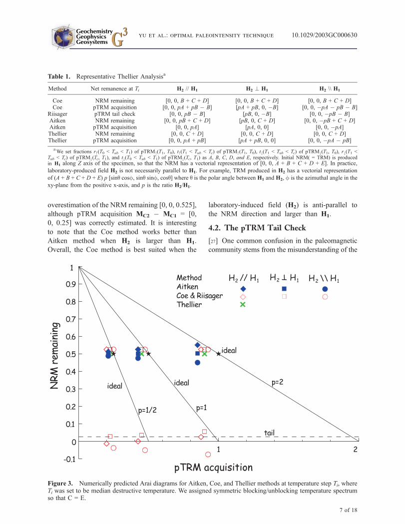
overestimation of the NRM remaining [0, 0, 0.525],

although pTRM acquisition MC2 � MC1 = [0,

0, 0.25] was correctly estimated. It is interesting

to note that the Coe method works better than

Aitken method when H2 is larger than H1.

Overall, the Coe method is best suited when the

laboratory-induced field (H2) is anti-parallel to

the NRM direction and larger than H1.

4.2. The pTRM Tail Check

[27] One common confusion in the paleomagnetic

community stems from the misunderstanding of the

Table 1. Representative Thellier Analysisa

Method Net remanence at Ti H2 // H1 H2 ? H1 H2 \\ H1

Coe NRM remaining [0, 0, B + C + D] [0, 0, B + C + D] [0, 0, B + C + D]Coe pTRM acquisition [0, 0, pA + pB � B] [pA + pB, 0, �B] [0, 0, �pA � pB � B]

Riisager pTRM tail check [0, 0, pB � B] [pB, 0, �B] [0, 0, �pB � B]Aitken NRM remaining [0, 0, pB + C + D] [pB, 0, C + D] [0, 0, �pB + C + D]Aitken pTRM acquisition [0, 0, pA] [pA, 0, 0] [0, 0, �pA]Thellier NRM remaining [0, 0, C + D] [0, 0, C + D] [0, 0, C + D]Thellier pTRM acquisition [0, 0, pA + pB] [pA + pB, 0, 0] [0, 0, �pA � pB]

aWe set fractions r"(T0 < Tub < T1) of pTRM"(T1, T0), t"(T1 < Tub < Tc) of pTRM"(T1, T0), t#(T1 < Tub < Tc) of pTRM#(T1, T0), r#(T1 <

Tub < Tc) of pTRM#(Tc, T1), and t#(T0 < Tub < T1) of pTRM#(Tc, T1) as A, B, C, D, and E, respectively. Initial NRM( = TRM) is producedin H1 along Z axis of the specimen, so that the NRM has a vectorial representation of [0, 0, A + B + C + D + E]. In practice,

laboratory-produced field H2 is not necessarily parallel to H1. For example, TRM produced in H2 has a vectorial representation

of (A + B + C + D + E) p [sinq cosf, sinq sinf, cosq] where q is the polar angle between H1 and H2, f is the azimuthal angle in the

xy-plane from the positive x-axis, and p is the ratio H2/H1.

ideal

tail

1 2-0.1

0.1

0.2

0.3

0.4

0.5

0.6

0.7

0.8

0.9H2 // H1 H2 H1 H2 \\ H1

pTRM acquisition

0

NR

M r

emai

ning

1MethodAitkenCoe & RiisagerThellier

T

idealideal p=2

p=1p=1/2

Figure 3. Numerically predicted Arai diagrams for Aitken, Coe, and Thellier methods at temperature step Ti, whereTi was set to be median destructive temperature. We assigned symmetric blocking/unblocking temperature spectrumso that C = E.



7 of 18

two different types of pTRM tails. The pTRM tail

check method was designed to detect the pTRM"tail (t", B in Figure 2b) and does so. However, it

fails to detect reliably the pTRM# tail (t#, C in

Figure 2c [see Shcherbakov and Shcherbakova,

2001]). t# is measurable only when specimens are

subjected to heating to the Curie temperature. In

other words, although it is embedded in the TRM,

the tails of the pTRM#s remain invisible during

Thellier analysis, yet can bias the result.

[28] The outcome of our pTRM tail analysis is

summarized in Table 2 for some representative

situations. In Figure 3, we set a t" as B = [0, 0,

0.025]. It is surprising that the pTRM tail check

detects the proper tail only when H2 is parallel to

and twice as large as H1. Depending on the

direction of H2 or magnitude of p, the pTRM tail is

either overestimated or underestimated. It is

interesting that the quality of data in paleointensity

determinations improves as H2 makes a larger

angle to the NRM while the pTRM tail is better

detected whenH2 is parallel to the NRM (Figure 3).

In fact, when H2 is perpendicular to the NRM,

pTRM tails are overestimated while H2 anti-

parallel to NRM underestimates tails.

[29] Why does the tail check fail to properly

detect the pTRM" tail? It is not because the

pTRM"(pB) is absent but because pB is masked

by a preexisting pTRM" tail B. Initially the

pTRM" tail was embedded in the total TRM as

[0, 0, B]. This inherited fraction systematically

deflects pB. In fact, the pTRM tail check analysis

detects the vectorial difference between the two

(= MC1 � MC1). As a result, the pTRM tail

check cannot properly estimate the amount of pB

(Figure 3, Table 2).

4.3. Aitken Method

[30] In Figure 3, the Aitken method is always

worse than the Thellier method, but often

behaves better than the Coe method when H2 is

parallel to the NRM and p < 1. When H2 is larger

than H1, the Aitken method substantially under-

estimates the pTRM acquisition and shows a

significant angular dependence. The only merit

that the Aitken method offers is the exact estimate

of the NRM remaining when H2 is perpendicular to

NRM (Figure 3).

4.4. Thellier Method

[31] The Thellier method always yields a precise

estimate of the NRM remaining, but underesti-

mates the pTRM acquired (Figure 3). The classical

Thellier method is unique in the sense that both

pTRM acquisition and NRM remaining are inde-

pendent of the direction of H2. It is free from

angular dependence because of its experimental

design. In the Aitken or Coe methods, tails

acquired by laboratory reheating are only affecting

the pTRM acquisition steps (in-field heating). On

the other hand, in the Thellier analysis, two pTRMs

in opposite directions are equally influenced by

pTRM" tails. As a result, the Thellier method is

independent of the direction of H2.

4.5. Further Comparisons

[32] It has been reported that high- and low-temper-

ature tails are roughly symmetric when viscous

remanent magnetizations (VRMs) or pTRMs are

produced at intermediate (300–400�C) tempera-

tures [Dunlop and Ozdemir, 2000, 2001]. This

interesting observation has been extended to include

the entire blocking and unblocking temperature

spectrum up to Curie point of magnetite [Fabian,

2001; Shcherbakov and Shcherbakova, 2001].

However, a symmetric distribution of blocking/

unblocking temperature spectra remains to be tested

particularly at low (<300�C) and high (>500�C)temperatures. It is therefore worth investigating

the outcome of our thought experiments if the

high and low temperature tails are not symmetric.

[33] We have assumed symmetry of pTRM tails in

Figure 3 so that C = E = 0.05, but the total high-

temperature tails exceeded a low-temperature tail

because of fraction B (= 0.025). Note that symme-

Table 2. Summary of pTRM Tail Checka

p H2 // H1 H2 ? H1 H2 \\ H1

1 [0, 0, 0] [B, 0, �B] [0, 0, �2B]2 [0, 0, B] [2B, 0, �B] [0, 0, �3B]1/2 [0, 0, �B/2] [B/2, 0, �B] [0, 0, �3B/2]

aNotations as in Table 1.



8 of 18

ideal

tail

1 2-0.1

0.1

0.2

0.3

0.4

0.5

0.6

0.7

0.8

0.9

pTRM acquisition

0

NR

M r

em

aini

ng1

tail

1 2-0.1

0.1

0.2

0.3

0.4

0.5

0.6

0.7

0.8

0.9

pTRM acquisition

0

NR

M r

em

aini

ng

1

a)

b)

ideal

ideal

ideal

idealideal

p=2

p=2

p=1

p=1p=1/2

p=1/2

H2 // H1 H2 H1 H2 \\ H1MethodAitkenCoe & RiisagerThellier

T

H2 // H1 H2 H1 H2 \\ H1MethodAitkenCoe & RiisagerThellier

T

Figure 4. Numerically predicted Arai diagrams for Aitken, Coe, and Thellier methods at temperature step Ti, whereTi was set to be median destructive temperature. In this calculation, we allowed a skewed distribution of unblockingtemperature spectrum. (a) B = 0.03, C = 0.06, E = 0.04; (b) B = 0.02, C = 0.04, E = 0.06.



9 of 18

try in rock magnetism represents identical magni-

tudes between C and E (only for pTRM#s) and not

between B + C and E. In fact, the B fraction has

been ignored. In Figure 4, we allowed an asym-

metric distribution of the blocking/unblocking

relation. At first, we set the high-temperature tails

(B = 0.03, C = 0.06) larger than a low temperature

tail (E = 0.04) (Figure 4a). Second, a dominant

low-temperature tail was set (B = 0.02, C = 0.04,

E = 0.06) (Figure 4b). Compared to Figure 3, each

datapoint in Figure 4a overestimates the NRM

remaining but underestimates the pTRM acquisi-

tion. As a result, each datapoint shifts up and to the

left in the Arai plot. For a dominant low-temper-

ature tail (E > C), underestimation of both NRM

remaining and pTRM acquisition worsens, result-

ing in a more concave down Arai plot (Figure 4b).

5. General Formulations

5.1. Paleointensity Formulations

[34] In sections 3 and 4, a double heating Thellier-

type experiment with a single temperature step was

investigated. In practical Thellier analyses, we

carry out stepwise double heatings at many tem-

perature steps. An empirical formulation of a

realistic Thellier experiment is in fact very com-

plicated. For convenience, we adopt a similar

convention as in the previous sections so that

TRM is produced along the z axis of the specimen.

For example, the zero-field heating/cooling to Tierases the unblocking temperature spectrum (Tub <

Ti) while in-field heating/cooling to Ti produces a

pTRM"(Ti, T0). The total TRM is the summation of

sequential pTRM#s:

TRM ¼Xci¼1

0; 0; pTRM# Ti; Ti�1ð Þ� �

: ð5Þ

According to equation (4), we can generalize

equation (5) as follows:

TRM ¼Xci¼1

0; 0; r" Ti; Ti�1ð Þ�

þt" Ti;Ti�1ð Þ þ t#1 Ti;Ti�1ð Þ

þ t#2 Ti;Ti�1ð Þ� ð6Þ

where r" is the reciprocal fraction of pTRM", t" is a

high temperature tail of pTRM", t#1 is a high-

temperature tail of pTRM#, t#2 is a low-temperature

tail of pTRM#, and temperatures within parenthesis

are Tbs. Each fraction was sub-divided according

to their corresponding unblocking temperature

spectrum.

[35] In the Coe method, the first (zero-field) heat-

ing and cooling to Tj erases fractions whose

unblocking tempartures are less than Tj, leaving

the remaining NRM

MCi1 ¼Xci¼jþ1

0; 0; r" Ti�1 < Tub < Tið Þ þ t#1 Ti�1 < Tub < Tið Þ�

þ t#2 Ti�1 < Tub < Tið Þ�þ F: ð7Þ

For convenience, we denote the pTRM" tail as F,

F ¼Xci¼jþ1

0; 0; t" Ti�1 < Tub < Tið Þ� �

: ð8Þ

[36] The second (in-field) heating/cooling to Tjproduces pTRM" (Tj, T0), yielding

MCi2 ¼ MCi1 � F þXji¼1

r" Ti�1 < Tub < Tið Þ

þXji¼1

t" Ti;Ti�1ð Þ!

� p sin q cosf; p sin q sinf; p cos q½ �: ð9Þ

The net pTRM acquisition at Tj is,

MCi2 �MCi1 ¼Xji¼1

r" Ti�1 < Tub < Tið Þ

þXji¼1

t" Ti; Ti�1ð Þ!

� p sin q cosf; p sin q sinf; p cos q½ � � F: ð10Þ

In the tail check method, a third (zero field)

heating/cooling to Tj yields,

MCi3 ¼ MCi1 þXji¼1

t" Ti;Ti�1ð Þ

� p sin q cosf; p sin q sinf; p cos q½ � � F: ð11Þ

Thus the measured pTRM tail is,

MCi3 �MCi1 ¼Xji¼1

t" Ti;Ti�1ð Þ

� p sin q cosf; p sin q sin q; p cos q½ � � F: ð12Þ

[37] As shown in sections 3.4, pTRM acquisition at

Tj in the Aitken method is equivalent to MC1 in the

Coe method and the NRM remaining at Tj in the

Aitken method is equivalent to MC3 in the Coe



10 of 18

method. As a result, in the Aitken method, the

NRM lost and the net pTRM acquired at Tjare MAi2 = MCi3 and MAi1 = MCi2 � MCi3 ,

respectively.

[38] In the classical Thellier method, the first in-

field (H2) heating yields, MTi1 = MCi2. The second

in-field (–H2) heating yields,

MTi2 ¼ MCi1 � F �Xji¼1

r" Tub < Tið Þþ Xj

i¼1

t" Ti; Ti�1ð Þ!


Half of the vector sum of MTi1 and MTi2 is the

NRM remaining at Tj ( = MCi1 � F). Half of the

vector difference between MTi1 and MTi2 is the net

pTRM acquisition at Tj,

MTi1 �MTi2 ¼Xji¼1

r" Tub < Tið Þ þ Xj

i¼1

t" Ti; Ti�1ð Þ!


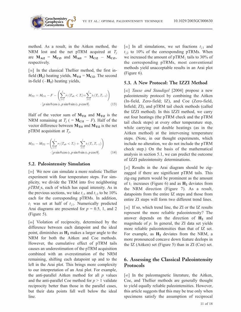
5.2. Paleointensity Simulation

[39] We now can simulate a more realistic Thellier

experiment with four temperature steps. For sim-

plicity, we divide the TRM into five neighboring

pTRM#s, each of which has equal intensity. As in

the previous sections, we take t#1 and t#2 to be 10%

each for the corresponding pTRMs. In addition,

t" was set at half of t#1. Numerically predicted

Arai diagrams are presented for p = 0.5, 1, and 2

(Figure 5).

[40] Violation of reciprocity, determined by the

difference between each datapoint and the ideal

point, diminishes as H2 makes a larger angle to the

NRM for both the Aitken and Coe methods.

However, the cumulative effect of pTRM tails

causes an underestimation of the pTRM acquisition

combined with an overestimation of the NRM

remaining, shifting each datapoint up and to the

left in the Arai plot. This brings more complexity

to our interpretation of an Arai plot. For example,

the anti-parallel Aitken method for all p values

and the anti-parallel Coe method for p > 1 validate

reciprocity better than those in the parallel cases,

but their data points fall well below the ideal

line.

[41] In all simulations, we set fractions t#1 and

t#2 to 10% of the corresponding pTRMs. When

we increased the amount of pTRM# tails to 30% of

the corresponding pTRMs, most conventional

methods yield unacceptable results in an Arai plot

(Figure 6).

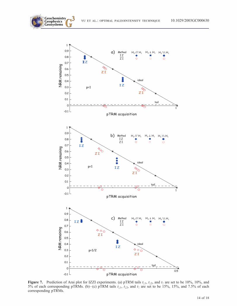
5.3. A New Protocol: The IZZI Method

[42] Tauxe and Staudigel [2004] propose a new

paleointensity protocol by combining the Aitken

(In-field, Zero-field; IZ), and Coe (Zero-field,

Infield; ZI), and pTRM tail check methods (called

the IZZI method). In this IZZI method, we carry

out four heatings (the pTRM check and the pTRM

tail check steps) at every other temperature step,

while carrying out double heatings (as in the

Aitken method) at the intervening temperature

steps. (Note, in our thought experiments, which

include no alteration, we do not include the pTRM

check step.) On the basis of the mathematical

analysis in section 5.1, we can predict the outcome

of IZZI paleointensity determinations.

[43] Results in the Arai diagram should be zig-

zagged if there are significant pTRM tails. This

zig-zag pattern would be prominent as the amount

of t" increases (Figure 6) and as H2 deviates from

the NRM direction (Figure 7). As a result,

datapoints from the entire IZ steps and those from

entire ZI steps will form two different trend lines.

[44] If so, which trend line, the ZI or the IZ results

represent the more reliable paleointensity? The

answer depends on the direction of H2 and

magnitude of p. In general, the ZI data set yields

more reliable paleointensities than that of IZ set.

For example, as H2 deviates from the NRM, a

more pronounced concave down feature deelops in

the IZ (Aitken) set (Figure 5) than in ZI (Coe) set.

6. Assessing the Classical PaleointensityProtocols

[45] In the paleomagnetic literature, the Aitken,

Coe, and Thellier methods are generally thought

to yield equally reliable paleointensities. However,

this article suggests that this may be true only when

specimens satisfy the assumption of reciprocal



11 of 18

ideal

tail

1-0.1

0.1

0.2

0.3

0.4

0.5

0.6

0.7

0.8

0.9

pTRM acquisition

0

NR

M r

emai

ning

1

ideal

tail

2-0.1

0.1

0.2

0.3

0.4

0.5

0.6

0.7

0.8

0.9

pTRM acquisition

0

NR

M r

emai

ning

1

ideal

tail

0.5-0.1

0.1

0.2

0.3

0.4

0.5

0.6

0.7

0.8

0.9

pTRM acquisition

0

NR

M r

emai

ning

1

p=2

p=1

p=1/2

a)H2 // H1 H2 H1 H2 \\ H1Method

AitkenCoe & RiisagerThellier

T

b)H2 // H1 H2 H1 H2 \\ H1Method


T

c)H2 // H1 H2 H1 H2 \\ H1Method


T

Figure 5. Simulated Arai plots for four-step Thellier analysis. pTRM tails t#1, t#2, and t" are set to be 10%, 10%,and 5% of each corresponding pTRMs. (a) p = 1, (b) p = 2, (c) p = 1/2.



12 of 18

ideal

tail

1-0.1

0.1

0.2

0.3

0.4

0.5

0.6

0.7

0.8

0.9

pTRM acquisition

0

NR

M r

emai

ning

1

ideal

tail

1 2-0.1

0.1

0.2

0.3

0.4

0.5

0.6

0.7

0.8

0.9

pTRM acquisition

0

NR

M r

emai

ning

1

ideal

tail

0.5-0.1

0.1

0.2

0.3

0.4

0.5

0.6

0.7

0.8

0.9

pTRM acquisition

0

NR

M r

emai

ning

1

p=1

p=2

p=1/2

a)H2 // H1 H2 H1 H2 \\ H1Method


T

b)H2 // H1 H2 H1 H2 \\ H1Method


T

c)H2 // H1 H2 H1 H2 \\ H1Method


T

Figure 6. Simulated Arai plots for four-step Thellier analysis. pTRM tails t#1, t#2, and t" are set to be 15%, 15%,and 7.5% of each corresponding pTRMs. (a) p = 1, (b) p = 2, (c) p = 1/2.



13 of 18

ideal

tail

1-0.1

0.1

0.2

0.3

0.4

0.5

0.6

0.7

0.8

0.9

pTRM acquisition

0

NR

M r

emai

ning

1

ideal

tail

1-0.1

0.1

0.2

0.3

0.4

0.5

0.6

0.7

0.8

0.9

pTRM acquisition

0

NR

M r

emai

ning

1

ideal

tail

0.5-0.1

0.1

0.2

0.3

0.4

0.5

0.6

0.7

0.8

0.9

pTRM acquisition

0

NR

M r

emai

ning

1

p=1

p=1

p=1/2

II Z

Z I

H2 // H1 H2 H1 H2 \\ H1Method I Z Z I

Ta)


Tb)


Tc)

I Z

I Z

I Z

I Z

I Z

Z I

Z I

Z I

Z I

Z I

Figure 7. Prediction of Arai plot for IZZI experiments. (a) pTRM tails t#1, t#2, and t" are set to be 10%, 10%, and5% of each corresponding pTRMs. (b)–(c) pTRM tails t#1, t#2, and t" are set to be 15%, 15%, and 7.5% of eachcorresponding pTRMs.



14 of 18

blocking and unblocking temperatures. In practice,

only uniformly magnetized particles and perhaps

also particles whose remanence state is ‘‘flower’’

[see Schabes and Bertram, 1988; Tauxe et al.,

2002] satisfy reciprocity. Given that many geolog-

ical specimens have magnetic grains with more

complicated remanence states (vortex and multido-

main) for which reciprocity may not hold, how can

the assumption of reciprocity best be tested in

practice?

[46] The use of the Aitken method should be

restricted to the case when the magnitude of H2 is

smaller than H1. When H2 exceeds H1, the Aitken

method is the least satisfactory among the three

techniques considered here. In particular, the

Aitken method shows the most angular dependence

when p > 1 (Figures 3–6).

[47] Only the Thellier method is independent of

the direction of H2 (see section 4.4). Along

with the anti-parallel Coe method, the Thellier

method detects reciprocity better than other

techniques. However, we do not recommend the

classical Thellier method because it lacks the

pTRM check step (or it requires an extra heating

step, while the Aitken and Coe methods require a

single in-field heating at each pTRM check step).

The pTRM check step is essential to detect

alteration of the specimen during the experiment,

hence is a requirement in all modern paleointensity

investigations.

[48] The Coe method seems to be the most robust

technique for practical use of the three classical

methods considered here. It is interesting that as the

angle between H2 and NRM increases, reciprocity

holds better but the accuracy of detecting proper

pTRM tails diminishes (Figures 3–6). In the case

of p > 1 for parallel Aitken and Coe methods, data

points shift nearly along the ideal line, resulting in

fairly reliable paleointensity although reciprocity

was mostly violated. In other words, depending on

the value of p, the angle of H2 should be

determined in Coe method. Perhaps surprisingly,

the Coe method works best when H2 makes a large

angle to the NRM for p < 1.

[49] An anti-parallel Coe method (H2 being anti-

parallel to NRM) is highly recommended for p < 1

to determine the most reliable paleointensity.

However, this requires a major correction in

modern sample selection criteria. In the nonparallel

Coe method, pTRM" tails will likely deflect

the NRM toward the direction of H2. Because

both-pTRM" and its tail have a temperature

dependence [Shcherbakov and Shcherbakova,

2001; Yu and Dunlop, 2003], the amount of

deflection will vary as the temperature steps change.

[50] Because the pTRM tail has a pronounced

angular dependence and can only be detected

reliably when H2 is parallel to the NRM with p =

2 (section 4.2), the pTRM tail check is of limited

use in practical paleointensity determinations. The

conventional pTRM tail check [Riisager and

Riisager, 2001] detects the vectorial difference

between the high-temperature tails of pTRM" and

the preexisting high-temperature tails that are

embedded in TRM. Therefore the pTRM tail check

falls short in its intended purpose.

7. Discussion and Conclusions

[51] In rock magnetism, a linear weak-field depen-

dence of TRM has been thoroughly tested [e.g.,

Thellier, 1938; Neel, 1955; Levi and Merrill, 1976;

Day, 1977; Tucker and Reilly, 1980; Shcherbakov et

al., 1993; Dunlop and Argyle, 1997; Muxworthy

and McClelland, 2000]. On the basis of these

experimental confirmations, use of arbitrary

p values has been commonly accepted in paleoin-

tensity determination as long as jH2j is less than

�100 mT. However, on the basis of our mathema-

tical model, results in Tables 1–2 and Figures 3–6

strongly suggest that value of H2 should be

restricted to less than H1. Otherwise, it is likely

to that the paleointensity will be less reliable.

[52] Using H2 < H1 has other advantages as well.

Within the experimental uncertainty of each data

point in real Thellier analyses, it is very likely that

the Aitken, Coe, and classical Thellier methods

will yield indistinguishable outcomes for specimens

with negligible (<10%) pTRM" tails (Figure 3). In

practice, however, the angular dependence of the

Aitken and Coe techniques are experimentally

resolvable when H2 > H1 (Figures 3 and 4) or when

specimens contain substantial tails (Figure 6).



15 of 18

[53] As the amount of the pTRM" tail increases

from 5% (Figure 5) to 7.5% (Figure 6), a more

pronounced concave downward feature develops in

the Arai diagram. In Figure 6, the paleointensity is

demonstrably unreliable in most cases we investi-

gated. In other words, pTRM" tails more than 5%

at any temperature intervals would significantly

compromise the quality of paleointensity. Indeed,

measuring the pTRM" tail is a good exercise in

preselecting suitable samples for paleointensity

determinations, as suggested by Shcherbakova et

al. [2000] and Shcherbakov and Shcherbakova

[2001].

[54] The Aitken method is in some respects similar

to the pTRM tail check method but does not carry

out the first zero field heating. Their physical

equivalency is mathematically supported because

MA1 = MC2 and MA2 = MC3. However, the

outcome on the Arai diagram is quite different.

This apparent paradox results not from difference

in experimental design but from a difference in

data processing. For example, the NRM remaining

at T1 is MA2 in the Aitken method but MC1 in the

Coe method (and not MC3) and the pTRM

acquisition at T1 is MA1 � MA2 in the Aitken

method but MC2 � MC1 in the Coe method (and

not MC2 � MC3).

[55] In section 3.1, we stated that the in-field

step at T1 produces a pTRM" (T1, T0) that

magnetize/remagnetizes fractions A and B. There

is a possibility that producing a pTRM" (T1, T0)

from a demagnetized state and from other par-

tially remagnetized states may induce different

pTRMs. Although the initial state dependence of

pTRM intensity has been reported [Shcherbakov

et al., 2001], its outcome on partially demagne-

tized/remagnetized samples has not been fully

observed. In a similar vein, thermal stability of

the pTRM tail [Shcherbakov and Shcherbakova,

2001] has raised another puzzle in the context of

Thellier experiments. However, any secure con-

clusion cannot be extracted from the current state

of experimental evidence because of the scalar

nature of the published experiments where

pTRMs are parallel to laboratory produced

NRMs. Intensity of pTRM and its tail and the

thermal stability of both during Thellier analysis

should be analyzed vectorially because pTRM

can often be masked/amplified by existing other

tails inherited from different magnetization [Yu

and Dunlop, 2003; this study].

[56] In practical Thellier-type experiments, we do

not know the initial field H1, nor do we know the

remanence direction at every step, as the initial

NRM may consist of more than one component.

Therefore perhaps the best strategy is to have

multiple specimens with randomly oriented NRM

with respect to the laboratory field H2. It is also

wise to use a relatively low laboratory field, say

10–15 mT, which is lower than most measured

paleointensity values. Use of the IZZI protocol

under these conditions ensures that reciprocity has

been fully tested and that reproducibility among

multiple specimens per cooling unit provides a

robust estimate for the paleointensity. Relying

solely on linearity of the Arai plot, pTRM checks,

and even pTRM tail checks is insufficient to

guarantee a reliable result.

Acknowledgments

[57] This research was supported by NSF grant EAR0229498

to L. Tauxe. We benefited from fruitful discussions with Peter

Selkin. D. V. Kent, V. Shcherbakov, and an anonymous

referees provided helpful reviews. We thank Jason Steindorf

for help with the measurements.

References

Aitken, M. J., A. L. Allsop, G. D. Bussell, and M. B. Winter

(1988), Determination of the intensity of the Earth’s mag-

netic field during archeological times: Reliability of the thel-

lier technique, Rev. Geophys., 26, 3–12.

Biggin, A. J., and H. N. Bohnel (2003), A method to reduce

the curvature of arai plots produced during Thellier paleoin-

tensity experiments performed on multidomain grains, Geo-

phys. J. Int., 155, F13–F19.

Carlut, J., and D. V. Kent (2002), Grain size dependent

paleointensity results from very recent mid-oceanic ridge

basalts, J. Geophys. Res., 107(B3), 2049, doi:10.1029/

2001JB000439.

Carvallo, C., O. Ozdemir, and D. J. Dunlop (2004), Paleoin-

tensity determinations, paleodirections, and magnetic proper-

ties of basalts from the Emperor seamounts, Geophys. J. Int.,

156, 29–38.

Coe, R. S. (1967), Paleointensities of the Earth’s magnetic

field determined from Tertiary and Quaternary rocks, J. Geo-

phys. Res., 72, 3247–5281.

Day, R. (1977), TRM and its variation with grain size,

J. Geomag. Geoelectr., 29, 233–265.



16 of 18

Dunlop, D. J., and K. S. Argyle (1997), Thermoremanence,

anhysteretic remanence and susceptibility of submicron mag-

netites: Nonlinear field dependence and variation with grain

size, J. Geophys. Res, 102, 20,199–20,210.

Dunlop, D. J., and O. Ozdemir (2000), Effect of grain size and

domain state on thermal demagnetization tails, Geophys.

Res. Lett., 27, 1311–1314.

Dunlop, D. J., and O. Ozdemir (2001), Beyond Neel’s theories:

Thermal demagnetization of narrow-band partial thermore-

manent magnetization, Phys. Earth Planet. Int., 126, 43–57.

Dunlop, D. J., and G. F. West (1969), An experimental evalua-

tion of single domain theories, Rev. Geophys., 7, 709–757.

Fabian, K. (2001), A theoretical treatment of paleointensity

determination experiments on rocks containing pseudo-sin-

gle or multi domain magnetic particles, Earth Planet. Sci.

Lett., 188, 45–48.

Kono, M. (1974), Intensities of the Earth’s magnetic field

about 60 m.y. ago determined from the Deccan Trap basalts,

India, J. Geophys. Res., 79, 1135–1141.

Kono, M., and N. Ueno (1977), Paleointensity determination

by a modified Thellier method, Phys. Earth Planet. Inter.,

13, 305–314.

Krasa, D., C. Heunemann, R. Leonhardt, and N. Petersen

(2003), Experimental procedure to detect multidomain rema-

nence during Thellier-Thellier experiments, Phys. Chem.

Earth, 28, 681–687.

Levi, S. (1979), The additivity of partial thermoremanent mag-

netization in magnetite, Geophys. J.R. Astron. Soc, 59, 205–

218.

Levi, S., and R. T. Merrill (1976), A comparison of ARM and

TRM in magnetite, Earth Planet. Sci. Lett., 32, 171–184.

McClelland, E., and N. Sugiura (1987), A kinematic model of

TRM acquisition in multidomain magnetite, Phys. Earth

Planet. Int., 46, 9–23.

Muxworthy, A., and E. McClelland (2000), The causes of low-

temperature demagnetization of remanence in multidomain

magnetite, Geophys. J. Int., 140, 115–131.

Nagata, T., Y. Arai, and K. Momose (1963), Secular variation

of the geomagnetic total force during the last 5000 years,

J. Geophys. Res., 68, 5277–5282.

Neel, L. (1955), Some theoretical aspects of rock-magnetism,

Adv. Phys, 4, 191–243.

Ozima, M., and M. Ozima (1965), Origin of thermoremanent

magnetization, J. Geophys. Res, 70, 1363–1369.

Riisager, P., and J. Riisager (2001), Detecting multidomain

magnetic grains in thellier palaeointensity experiments,

Phys. Earth Planet. Inter., 125, 111–117.

Riisager, J., M. Perrin, P. Riisager, and G. Ruffet (2000),

Paleomagnetism, paleointensity and geochronology of mio-

cene basalts and baked sediments from Velay Oriental,

French Massif Central, J. Geophys. Res, 105, 883–896.

Riisager, P., J. Riisager, N. Abrahamsen, and R. Waagstein

(2002), Thellier palaeointensity experiments on faroes flood

basalts: Technical aspects and geomagnetic implications,

Phys. Earth Planet. Inter., 131, 91–100.

Schabes, M. E., and H. N. Bertram (1988), Magnetization

processes in ferromagnetic cubes, J. Appl. Phys., 64,

1347–1357.

Selkin, P., and L. Tauxe (2000), Long-term variations in

paleointensity, Philos. Trans. R. Astron. Soc., A358, 1065–

1088.

Shaw, J. (1974), A new method of determining the magnitude

of the paleomanetic field application to 5 historic lavas and

five archeological samples, Geophys. J. R. Astron. Soc., 39,

133–141.

Shcherbakov, V. P., and V. Shcherbakova (2001), On the sta-

bility of the Thellier method of paleointensity determination

on pseudo-single-domain and multidomain grains, Geophys.

J. Int., 146, 20–30.

Shcherbakov, V., E. McClelland, and V. Shcherbakova (1993),

A model of multidomain thermoremanent magnetization

incorporating temperature-variable domain structure, J. Geo-

phys. Res, 98, 6201–6214.

Shcherbakova, V., V. Shcherbakov, and F. Heider (2000),

Properties of partial thermoremanent magnetization in

PSD and MD magnetite grains, J. Geophys. Res, 105,

767–782.

Shcherbakov, V. P., V. Shcherbakova, Y. K. Vinogradov, and

F. Heider (2001), Thermal stability of pTRM created from

different magnetic states, Phys. Earth Planet. Int., 126,

59–73.

Sholpo, L. E., V. A. Ivanov, and G. P. Borisova (1991), Ther-

momagnetic effects of reorganization of domain structure,

Izv. Acad. Sci. USSR, 27, 617–623.

Smith, P. (1967), The intensity of the Tertiary geomagnetic

field, Geophys. J. Roy. Astron. Soc, 12, 239–258.

Tauxe, L., and J. Love (2003), Paleointensity in Hawaiian

Scientific Drilling Project Hole (HSDP2): Results from

submarine basaltic glass, Geochem. Geophys. Geosyst.,

4(2), 8702, doi:10.1029/2001GC000276.

Tauxe, L., and H. Staudigel (2004), Strength of the geomag-

netic field in the Cretaceous Normal Superchron: New data

from submarine basaltic glass of the Troodos Ophiolite, Geo-

chem. Geophys. Geosyst., p. in press.

Tauxe, L., H. Bertram, and C. Seberino (2002), Physical inter-

pretation of hysteresis loops: Micromagnetic modelling of

fine particle magnetite, Geochem. Geophys. Geosyst.,

3(10), 1055, doi:10.1029/2001GC000241.

Thellier, E. (1938), Sure l’aimantation des teres cuites et ses

applications g’eophysique, Ann. Inst. Phys. Globe Univ.

Paris, 16, 157–302.

Thellier, E., and O. Thellier (1959), Sur l’intensite du champ

magnetique terrestre dans le passe historique et geologique,

Ann. Geophys., 15, 285–378.

Tucker, P., and W. O. Reilly (1980), The acquisition of TRM

by MD single crystal titanomagnetite, Geophys. J. R. Astron.

Soc., 60, 21–36.

Valet, J.-P. (2003), Time variations in geomagnetic intensity,

Rev. Geophys., 41(1), 1004, doi:10.1029/2001RG000104.

Valet, J.-P., and E. Herrero-Bervera (2000), Paleointensity

experiments using alternating field demagnetization, Earth

Planet. Sci. Lett., 177, 43–58.

Valet, J. P., E. Tric, E. Herrero-Bervera, L. Meynadier, and

J. P. Lockwood (1998), Absolute paleointensity from

Hawaiian lavas younger than 35 ka, Earth Planet. Sci.

Lett., 177, 19–32.



17 of 18

van Zijl, J. S. U., K. W. T. Graham, and A. L. Hales (1962),

The paleomagnetism of the Stormberg lavas, 2. the behavior

of the Earth’s magnetic field during a reversal, Geophys. J.

R. Astron. Soc., 7, 169–182.

Vinogradov, Y. K., and G. P. Markov (1989), On the effect of

low temperature heating on the magnetic state of multido-

main magnetite(in Russian), Investigations in Rock Magnet-

ism and Paleomagnetism, pp. 31–39, Inst. of Phys. of the

Earth, Moscow.

Walton, D., J. Shaw, J. Share, and J. Hakes (1992), Microwave

demagnetization, J. Appl. Phys., 71, 1549–1551.

Wilson, R. L. (1961), Paleomagnetism in northern Ireland:

1, the thermoremanent magnetization of natural magnetic

moments in rocks, Geophys. J. R. Astron. Soc, 5, 45–

58.

Yu, Y., and D. J. Dunlop (2001), Paleointensity determination

on the late precambrian Tudor Gabbro, Ontario, J. Geophys.

Res, 106, 26,331–26,344.

Yu, Y., and D. J. Dunlop (2003), On partial thermoremanent

magnetization tail checks in Thellier paleointensity determi-

nation, J. Geophys. Res, 108(B11), 2523, doi:10.1029/

2003JB002420.



18 of 18

Toward an optimal geomagnetic field intensity determination technique

Documents