Total Lagrangian explicit dynamics finite element algorithm for computing soft tissue deformation

COMMUNICATIONS IN NUMERICAL METHODS IN ENGINEERINGCommun. Numer. Meth. Engng 2007; 23:121–134Published online 14 August 2006 in Wiley InterScience (www.interscience.wiley.com). DOI: 10.1002/cnm.887

Total Lagrangian explicit dynamics finite element algorithmfor computing soft tissue deformation

Karol Miller!,†, Grand Joldes, Dane Lance and Adam Wittek

Intelligent Systems for Medicine Laboratory, School of Mechanical Engineering, The University of WesternAustralia, 35 Stirling Highway, Crawley/Perth WA 6009, Australia

SUMMARY

We propose an efficient numerical algorithm for computing deformations of ‘very’ soft tissues (such asthe brain, liver, kidney etc.), with applications to real-time surgical simulation. The algorithm is based onthe finite element method using the total Lagrangian formulation, where stresses and strains are measuredwith respect to the original configuration. This choice allows for pre-computing of most spatial derivativesbefore the commencement of the time-stepping procedure.

We used explicit time integration that eliminated the need for iterative equation solving during thetime-stepping procedure. The algorithm is capable of handling both geometric and material non-linearities.The total Lagrangian explicit dynamics (TLED) algorithm using eight-noded hexahedral under-integratedelements requires approximately 35% fewer floating-point operations per element, per time step than theupdated Lagrangian explicit algorithm using the same elements.

Stability analysis of the algorithm suggests that due to much lower stiffness of very soft tissues thanthat of typical engineering materials, integration time steps a few orders of magnitude larger than what istypically used in engineering simulations are possible.

Numerical examples confirm the accuracy and efficiency of the proposed TLED algorithm. Copyright� 2006 John Wiley & Sons, Ltd.

Received 29 November 2005; Revised 7 May 2006; Accepted 12 May 2006

KEY WORDS: surgical simulation; soft tissues; finite element method; explicit time integration; totalLagrangian formulation

1. INTRODUCTION

There is wide international concern about the cost of meeting rising expectations for health care,particularly if large numbers of people require currently expensive procedures such as brain surgery.

!Correspondence to: Karol Miller, Intelligent Systems for Medicine Laboratory, School of Mechanical Engineering,The University of Western Australia, 35 Stirling Highway, Crawley/Perth WA 6009, Australia.

†E-mail: [email protected], http://www.mech.uwa.edu.au/ISML/

Contract/grant sponsor: Australian Research Council, Discovery Project; contract/grant numbers: DP0343112,DP0664534

Copyright � 2006 John Wiley & Sons, Ltd.

122 K. MILLER ET AL.

Costs can be reduced by using improved machinery to help surgeons perform these proceduresquickly and accurately, with minimal side effects. A novel partnership between surgeons andmachines, made possible by advances in computing and engineering technology, could overcomemany of the limitations of traditional surgery. By extending the surgeons’ ability to plan and carryout surgical interventions more accurately and with less trauma, computer-integrated surgery (CIS)systems could help to improve clinical outcomes and the efficiency of health care delivery. CISsystems could have a similar impact on surgery to that long since realized in computer-integratedmanufacturing (CIM).

Mathematical modelling and computer simulation have proved tremendously successful in engi-neering. Computational mechanics has enabled technological developments in virtually every areaof our lives. One of the greatest challenges for mechanists is to extend the success of computationalmechanics to fields outside traditional engineering, in particular to biology, biomedical sciences,and medicine [1].

The goal of surgical simulation research is to model and simulate deformable materials forapplications requiring real-time interaction. Medical applications for this include simulation-basedtraining, skills assessment and operation planning. A surgical simulator must predict the deforma-tion field within the organ, so that it can be displayed to the user, and the internal forces (stresses),so that reaction forces acting on surgical tools can be computed and conveyed to the user throughhaptic feedback.

For computational efficiency reasons most researchers in the surgical simulation community usemathematical models based on linear elasticity that allow pre-computation of solutions (Green’sfunctions). These models are incapable of providing realistic predictions of finite deformationsof the tissue, because the deformations are assumed to be infinitesimal. Linearity of the materialresponse is also assumed. Consequently, in such models the principle of superposition holds.However, years of experience accumulated by researchers working on the theory of elasticityand the finite element method have shown that the principle of superposition cannot be used forsystems undergoing large deformations. In the 1970s, when non-linear finite element procedureswere under development, many examples of inadequacy of linear theory were published, see e.g.References [2–4].

Zhuang [5], was probably the first to use updated Lagrangian explicit dynamics for real-time deformable object simulation. Picinbono et al. [6] used a similar algorithm, however theirimplementation of non-linear materials and viscoelasticity was, in our opinion, inferior to whatis available within commercial packages, such as LS Dyna [7]. Papers [5, 6] used meshes builtof linear tetrahedra, however they did not discuss problems related to volumetric locking. AlsoSzekely et al. [8] used explicit dynamics algorithms. Unfortunately, the details of their methodsare not given in the publication.

The efficient finite element algorithm, accounting for both geometric and material non-linearities,that alleviates the problems mentioned above, is presented in the next section. In Section 3, wepresent three computational examples. Section 4 contains discussion and conclusions.

2. METHODS

2.1. Total Lagrangian formulation of the finite element method

Various spatial discretization schemes are possible while using the finite element method [9]. Thegreat majority (if not all) of commercial finite element programs use the updated Lagrangian

Copyright � 2006 John Wiley & Sons, Ltd. Commun. Numer. Meth. Engng 2007; 23:121–134DOI: 10.1002/cnm

TOTAL LAGRANGIAN EXPLICIT DYNAMICS FINITE ELEMENT ALGORITHM 123

formulation, where all variables are referred to the current (i.e. from the end of the previoustime step) configuration of the system (Ansys [10], ABAQUS [11], ADINA [12], LS Dyna [13]).Therefore, Cauchy stress and Almansi (or logarithmic) strain are used. The advantage of thisapproach is the simplicity of incremental strain description. The disadvantage is that all derivativeswith respect to spatial co-ordinates must be recomputed in each time step, because the referenceconfiguration is changing. The reason for this choice is historical—at the time of solver developmentthe memory was expensive and caused more problems than actual speed of computations.

The first key idea in the finite element algorithm development is to use the total Lagrangianformulation of the finite element method, where all variables are referred to the original config-uration of the system. Second Piola–Kirchoff stress and Green strain are used. The disadvantageof this approach is the complicated description of finite strains resulting from the so-called initialdisplacement effect. However, the decisive advantage is that all derivatives with respect to spatialco-ordinates are calculated with respect to the original configuration and therefore can be pre-computed. Also, as rotation-invariant second Piola–Kirchoff stress is used, the necessity to rotate(Cauchy) incremental stresses before addition, present in updated Lagrangian formulation, is elim-inated. Therefore, the proposed algorithm performs significantly fewer mathematical operations ineach time step.

2.2. Explicit time integration of discretized equations of motion

The present study focuses on computing the deformation field and internal forces (stresses) withina soft organ during surgical procedure. This requires application of an efficient numerical schemewhen integrating equations of equilibrium (or dynamics) in time domain. Such integration canbe done using either implicit or explicit methods [14–16]. In implicit methods, the equationsof dynamics are combined with the time integration operator, and the displacements are founddirectly. In explicit methods, on the other hand, at first the accelerations are determined from theequations of dynamics and then integrated to obtain the displacements.

The most commonly used implicit integration methods, such as the Newmarks’ constant accel-eration method, are unconditionally stable [9]. This implies that their time step is limited only bythe convergence/accuracy considerations. However, the implicit methods require solution of a setof non-linear algebraic equations at each time step. Furthermore, iterations need to be performedfor each time step of implicit integration to control the error and prevent divergence. Therefore,the number of numerical operations per each time step can be three orders of magnitude largerthan for explicit integration [14]. Thus, ‘the advantage of implicit method for three-dimensional(transient) problems becomes marginal’ [9].

On the other hand, in explicit methods, such as the central difference method, treatment of non-linearities is very straightforward and no iterations are required. The global system of discretizedequations of motion to be solved at each time step is

Mun + K(un) · un =Rn (1)

where u is a vector of nodal displacements,M is a mass matrix, K is a stiffness matrix non-linearlydependent on the deformation (because geometrically non-linear procedure, suitable for computinglarge deformations, is used), and R is a vector of nodal (active) forces.

Using the central difference integration scheme we obtain:

un+1 = un + !tn+1un + 1/2!t2n+1un (2)



un+1 = un + 1/2!tn+1(un+1 + un) (3)

Kn · un = !iF(i)n = !

i

"

V (i)BTn Sn dV (4)

and #1

!t2M

$un+1 =Rn " !

iF(i)n " 1

!t2M(un"1 " 2un) (5)

where BTn is the strain–displacement matrix at step n and V (i) is the i th element volume.

The non-linear properties of the tissue are accounted for in the constitutive model (see e.g.References [17–21] for the brain, References [22–24] for liver and kidney) and included inthe calculation of nodal reaction forces F. We used lumped (diagonalized) mass matrix M thatmultiplies the unknown un+1. This rendered Equation (5) an explicit formula for the unknownun+1. Equations (4) and (5) imply that computations are done at the element level eliminating theneed for assembling the stiffness matrix K of the entire model. Thus, computational cost of eachtime step and internal memory requirements are substantially smaller for explicit than implicitintegration. It is worth noting that there is no need for iterations anywhere in the algorithm. Thisfeature makes the proposed algorithm suitable for real-time applications.

However, the explicit methods are only conditionally stable. Normally a severe restriction on thetime step size has to be included in order to receive satisfactory simulation results. For example,in car crash simulations conducted with explicit solvers the time step is usually in the order ofmagnitude of microseconds or even tenths of microseconds [25, 26].

The critical time step is equal to the smallest characteristic length Le of an element in the meshdivided by the dilatational wave speed c [7, 14, 27]:

!t ! Le

c(6)

For the eight-noded hexahedral element, the characteristic length is

Le = VAmax

(7)

where Amax is the area of the element’s largest face and V is the element’s volume.Stiffness of very soft tissue is very low [19]: e.g. stiffness of the brain is about eight orders of

magnitude lower than that of steel. Since the maximum time step allowed for stability is (roughlyspeaking) inversely proportional to the square root of Young’s modulus divided by the massdensity, it is possible to conduct simulations of brain deformation with much longer time stepsthan in typical dynamic simulations in engineering.

2.3. Description of TLED finite element algorithm

Pre-computation stage:

1. Load mesh and boundary conditions.2. For each element compute the determinant of the Jacobian det(J), spatial derivatives of

shape functions !h and linear (constant) strain–displacement matrices, t0BL0 (notation of

Reference [15] is used, where the left superscript represents the current time and the leftsubscript represents the time of the reference configuration—0 when total Lagrangian for-mulation is used).

3. Compute and diagonalize (constant) mass matrix 0M.



Initialization:1. Initialize nodal displacement 0u= 0, "!tu= 0, apply load for the first time step: forces or/and

prescribed displacements: !t R(k)i #" R(k)(!t) or/and !t u(k)

i #" d(!t).

Time stepping:Loop over elements:

1. Take element nodal displacements from the previous time step.2. Compute deformation gradient t0X.3. Calculate full strain–displacement matrix:

t0B

(k)L = t

0B(k)L0

t0X

T (8)

This matrix accounts for initial displacement effect.4. Compute second Piola–Kirchoff stress (vector) t

0S at integration points.5. Compute element nodal reaction forces

t F(m) ="

0V

t0B

TLt0S d

0V (9)

using Gaussian quadrature.

Making a (time) step:

1. Obtain net nodal reaction forces at time t , tF.2. Explicitly compute displacements using central difference formula

t+!t u(k)i = !t2

Mk

t (t Ri " t F (k)i ) + 2t u(k)

i " t"!t u(k)i (10)

where Mk is a diagonal entry in kth row of the diagonalized mass matrix, Ri is an externalnodal force, and !t is the time step.

3. Apply load for the next step: t+!t R(k)i #" R(k)(t + !t) or/and t+!t u(k)

i #" d(t + !t).

As can be seen, there is no need for solution of coupled equations anywhere in the algorithm.Computationally most expensive parts of the algorithm are the evaluation of the full strain–displacement matrix (Point 3 of the loop over elements) and of second Piola–Kirchoff stresses(Point 4 of the loop over elements). These computations must be conducted at every integrationpoint. That is why to achieve high computational efficiency under-integrated elements shouldbe used. For 3D problems the most efficient elements are eight-noded hexahedra with a singleintegration point (for an excellent description of the implementation of this element see LS DynaManual [7]). For this element the integral (9) can be simply evaluated as

t F(m) = 8t0BTLt0S det(

0J) (11)

As, for stability reasons, rather small time steps are used, the strain–displacement matrix doesnot change much during a few time steps. Our experience shows that it is sufficient to update itevery about 10 time steps. This leads to substantial computational efficiency improvement.

Accurate evaluation of stresses at integration points is essential for precise prediction of internalforces within the organ and computation of reaction forces acting on surgical tools. Therefore,appropriate constitutive models need to be applied. In case of hyperelastic models the second



Piola–Kirchoff stress can be evaluated as a derivative of the energy function with respect toGreen strain. When hyper-viscoelastic models, such as the Ogden-based one developed for thatbrain in Reference [19], are selected, an efficient recursive scheme should be implemented. Theimplementation method is explained in detail in Reference [28].

3. RESULTS

3.1. Stability analysis

Stability analysis of explicit integration schemes is very well developed for sets of linear differ-ential equations [29]. Most of the results are approximately valid for non-linear analysis as well.Nevertheless, we have conducted numerical experiments to ascertain the stability limits of theproposed algorithm.

We used 10 cm side cube meshed by 1000 eight-noded, single-integration-point hexahedra forthe test problem, as it makes defining boundary conditions and generating hexahedral meshessimple and has similar dimensions to the human brain. No hourglass control was used. The cube isdeformed by constraining one face, whilst the opposite face is displaced. The boundary conditionsare: constrained face: !x =!y =!z = 0; displaced face: !x = !z = 0, !y = d(t) (Figure 1). Massdensity of 1000 kg/m3 and Neo-Hookean material model with Young’s modulus in undeformedstate equal to 3000 Pa and Poisson’s ratio 0.49, which is approximately representative for thehuman brain, were used. The speed of sound in the bulk material is, therefore, approximately7m/s. For a mesh with 10 cubic elements per side, the critical time step, as predicted by a lineartheory [29] is

!tcrit =Lc

$ 0.0013 s

To obtain experimental verification of this prediction we computed the displacement of all nodeswith varying time steps. Above the critical time step the displacement increased dramatically asthe algorithm lost stability, Figure 2. Figure 3 shows the axial force during axial elongation of thecube computed with the time step size very close to the critical time step. Oscillations in the forcecan be seen as the algorithm becomes unstable.

Figure 1. Constrained elongation of a cube.



Figure 2. Logarithm of net nodal displacement with time step for 10 elements per side mesh.

Figure 3. Force versus time showing the onset of oscillations due to time step nearing the critical time step.

Therefore, it should be ensured that the time step does not exceed the critical time step predictedby the linear theory.

3.2. Numerical examples

In all numerical examples hexahedral meshes with and without hourglass control were used.The hourglass control algorithm uses artificial stiffness to treat the zero energy modes of the



Figure 4. Extension and compression of a cylinder.

under-integrated hexahedral elements, as described in Reference [30]. Results obtained with theproposed algorithm programmed in C [31] were compared to the ones obtained with ABAQUSStandard Version 6.5-1 finite element analysis package [11].

The computed deformed shape of the object was compared with the one obtained using ABAQUSStatic. The computed time evolution of the reaction force in one node was compared with the one



obtained using ABAQUS Dynamic/Implicit. In both cases default parameters of the ABAQUSsolver were used. A Neo-Hookean material model with Young’s modulus in undeformed stateequal to 3000 Pa, Poisson’s ratio 0.49 and mass density of 1000 kg/m3 was considered in all cases.A fully integrated eight-noded linear brick, hybrid, constant pressure element was used in ABAQUS.The maximum displacement was 0.02m in all cases and was applied using a loading curvegiven by

d(t) = (10 " 15t + 6t2)t3 (12)

where t is the relative time (varying from 0 to 1).

3.2.1. Extension and compression of a cylinder. The cylinder is deformed by constraining one face,whilst the opposite face is displaced. The boundary conditions are: constrained face: !x = !y =!z = 0; displaced face: !x =!y = 0, !z = d(t). The displacements are presented for a line ofnodes found at the intersection of the plane y = 0 with the lateral surface of the cylinder. Thereaction forces are presented for the node found in the middle of the displaced face, Figure 4.The results obtained with the proposed total Lagrangian explicit dynamics algorithm (TLED)are essentially the same as those obtained with ABAQUS indicating the appropriateness of thedeveloped methods. It is also clear that hourglass control is necessary to maintain the accuracy.Therefore, in the remaining examples hourglass control was used.

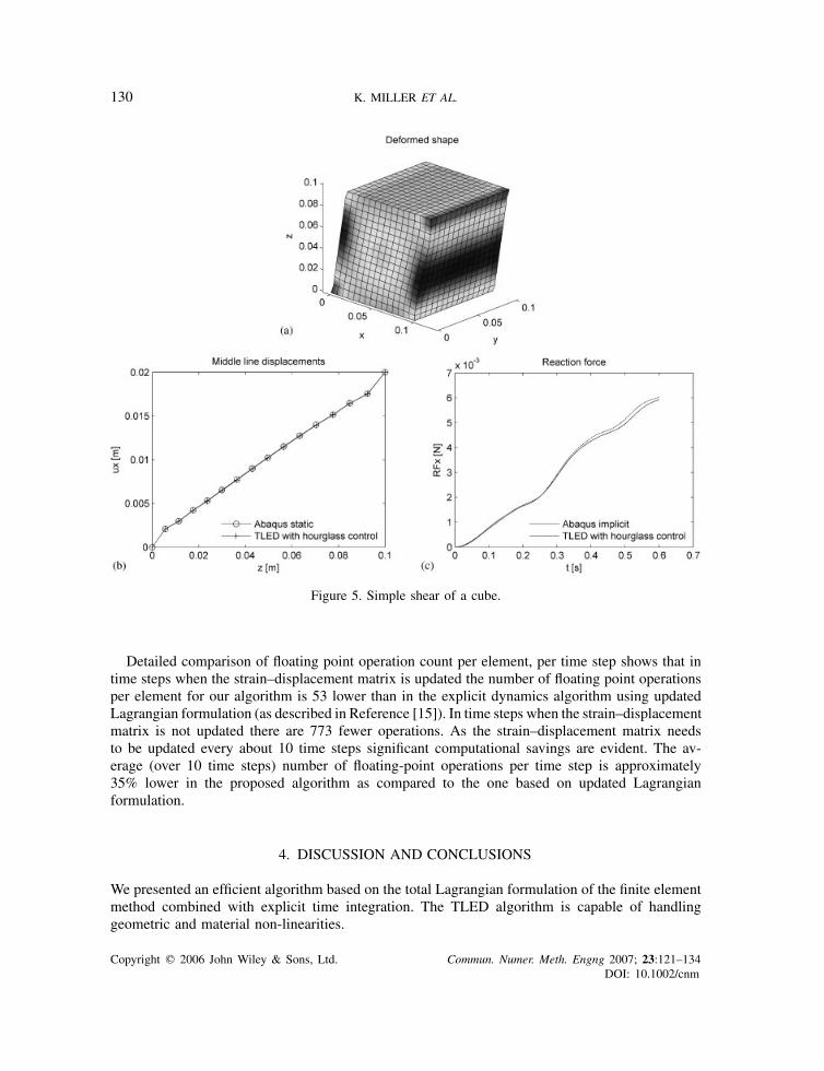
3.2.2. Simple shear of a cube. The cube is deformed by constraining one face, whilst the oppositeface is displaced. The boundary conditions are: constrained face: !x = !y = !z = 0; displacedface: !y = !z = 0, !x = d(t). The displacements are presented for a line of nodes found at theintersection of the plane y = 0.05 with the lateral surface of the cube. They agree well with thosecomputed with ABAQUS Static. The reaction forces are presented for the node found in the middleof the displaced face, Figure 5.

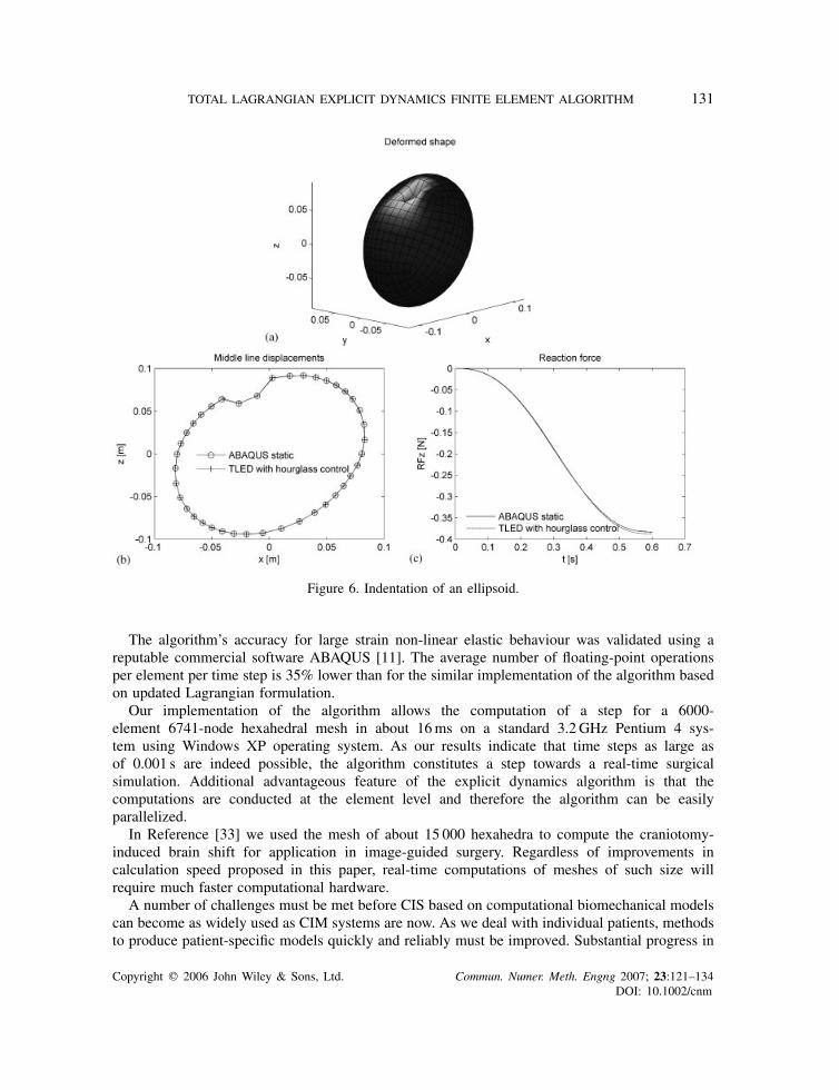
3.2.3. Indentation of an ellipsoid. The ellipsoid is deformed by constraining the lower half, whilstfour nodes are displaced in the z-direction. This is a rough approximation of indentation ofthe brain [32]. The boundary conditions are: constrained nodes: !x = !y = !z = 0; displacednodes: !x = !y = 0, !z = d(t). The displacements are presented for a line of nodes found at theintersection of the plane y = 0 with the surface of the ellipsoid. The reaction forces are presentedfor one of the displaced nodes, Figure 6.

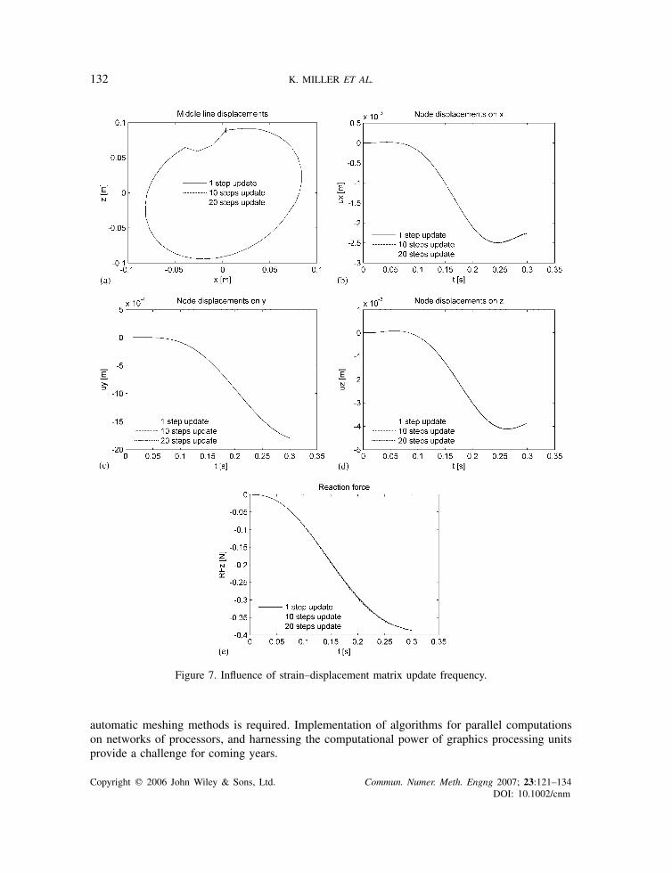
3.2.4. Influence of strain–displacement matrix update frequency. The strain–displacement matrixwas updated at different number of time-step intervals for the ellipsoid indentation experiment andthe obtained displacements, reaction forces and average time step were compared. The averagetime step was obtained by dividing the total computation time by the number of steps (1000 inthis case). The hourglass control algorithm takes about 5.9ms each step (using a standard 3.2GHzPentium 4 computer). The nodal displacements are presented for the node marked with a cross inthe middle line displacements (Figure 7). The reaction forces are presented for one of the displacednodes.

From these results it can be seen that the strain–displacement matrix can be updated at time stepintervals greater that 10, but the improvement in computation time for a greater update interval isminimal and the accuracy of the results starts to decrease (Table I).



Figure 5. Simple shear of a cube.

Detailed comparison of floating point operation count per element, per time step shows that intime steps when the strain–displacement matrix is updated the number of floating point operationsper element for our algorithm is 53 lower than in the explicit dynamics algorithm using updatedLagrangian formulation (as described in Reference [15]). In time steps when the strain–displacementmatrix is not updated there are 773 fewer operations. As the strain–displacement matrix needsto be updated every about 10 time steps significant computational savings are evident. The av-erage (over 10 time steps) number of floating-point operations per time step is approximately35% lower in the proposed algorithm as compared to the one based on updated Lagrangianformulation.

4. DISCUSSION AND CONCLUSIONS

We presented an efficient algorithm based on the total Lagrangian formulation of the finite elementmethod combined with explicit time integration. The TLED algorithm is capable of handlinggeometric and material non-linearities.



Figure 6. Indentation of an ellipsoid.

The algorithm’s accuracy for large strain non-linear elastic behaviour was validated using areputable commercial software ABAQUS [11]. The average number of floating-point operationsper element per time step is 35% lower than for the similar implementation of the algorithm basedon updated Lagrangian formulation.

Our implementation of the algorithm allows the computation of a step for a 6000-element 6741-node hexahedral mesh in about 16ms on a standard 3.2GHz Pentium 4 sys-tem using Windows XP operating system. As our results indicate that time steps as large asof 0.001 s are indeed possible, the algorithm constitutes a step towards a real-time surgicalsimulation. Additional advantageous feature of the explicit dynamics algorithm is that thecomputations are conducted at the element level and therefore the algorithm can be easilyparallelized.

In Reference [33] we used the mesh of about 15 000 hexahedra to compute the craniotomy-induced brain shift for application in image-guided surgery. Regardless of improvements incalculation speed proposed in this paper, real-time computations of meshes of such size willrequire much faster computational hardware.

A number of challenges must be met before CIS based on computational biomechanical modelscan become as widely used as CIM systems are now. As we deal with individual patients, methodsto produce patient-specific models quickly and reliably must be improved. Substantial progress in



Figure 7. Influence of strain–displacement matrix update frequency.

automatic meshing methods is required. Implementation of algorithms for parallel computationson networks of processors, and harnessing the computational power of graphics processing unitsprovide a challenge for coming years.



Table I. Influence of strain–displacement matrix updatefrequency on computation time.

Update frequency (steps) Average step time (ms)

1 22.65 16.5

10 15.720 15.4

ACKNOWLEDGEMENTS

The financial support of the Australian Research Council (Grant Nos. DP0343112, DP0664534) is gratefullyacknowledged. The second author was an Endeavor IPRS Scholar in Australia during the completion ofthis research. The first author would like to thank Professors Ivo Babuska, Graham Carey, Thomas Hughesand Leszek Demkowicz for very helpful discussion while visiting the University of Texas at Austin.

REFERENCES

1. Oden JT, Belytschko T, Babuska I, Hughes TJR. Research directions in computational mechanics. ComputerMethods in Applied Mechanics and Engineering 2003; 192:913–922.

2. Carey GF. A unified approach to three finite element theories for geometric nonlinearity. Journal of ComputerMethods in Applied Mechanics and Engineering 1974; 4(1):69–79.

3. Martin HC, Carey GF. Introduction to Finite Element Analysis: Theory and Application. McGraw-Hill Book Co:New York, 1973.

4. Oden JT, Carey GF. Finite Elements: Special Problems in Solid Mechanics. Prentice-Hall: Englewood Cliffs, NJ,1983.

5. Zhuang Y. Real-time simulation of physically realistic global deformations. Ph.D. Thesis, Department of ComputerScience, University of California, Berkley, 2000.

6. Picinbono G, Delingette H, Ayache N. Non-linear anisotropic elasticity for real-time surgery simulation. GraphicalModels 2003; 65:305–321.

7. Hallquist JO. LS-DYNA Theoretical Manual. Livermore Software Technology Corporation: Livermore, California,1998.

8. Szekely G, Brechbuhler C, Hutter R, Rhomberg A, Ironmonger N, Schmid P. Modelling of soft tissue deformationfor laparoscopic surgery simulation. Medical Image Analysis 2000; 4:57–66.

9. Belytschko T. An overview of semidiscretization and time integration procedures. In Computational Methods forTransient Analysis, Belytschko T, Hughes TJR (eds). North-Holland: Amsterdam, 1983; 1–66.

10. http://www.ansys.com/services/documentation/manuals.htm, ANSYS documentation. Accessed: 18/10/2005.11. ABAQUS. ABAQUS Online Documentation: Version 6.5-1. Hibbitt, Karlsson & Sorensen, Inc., 2004,

http://www.abaqus.com/products/products documentation.html12. www.adina.com, ADINA home page. Accessed: 22/11/2005.13. LS-DYNA. Keyword User’s Manual. Version 970. Livermore Software Technology Corporation: Livermore,

California, 2003.14. Belytschko T. A survey of numerical methods and computer programs for dynamic structural analysis. Nuclear

Engineering and Design 1976; 37:23–34.15. Bathe K-J. Finite Element Procedures. Prentice-Hall: Englewood-Cliffs, NJ, 1996.16. Crisfield MA. Non-linear dynamics. In Non-linear Finite Element Analysis of Solids and Structures. Wiley:

Chichester, 1998; 447–489.17. Miller K, Chinzei K. Constitutive modeling of brain tissue; experiment and theory. Journal of Biomechanics

1997; 30(11/12):1115–1121.18. Miller K. Constitutive model of brain tissue suitable for finite element analysis of surgical procedures. Journal

of Biomechanics 1999; 32:531–537.19. Miller K, Chinzei K. Mechanical properties of brain tissue in tension. Journal of Biomechanics 2002; 35:483–490.



20. Bilston L, Liu Z, Phan-Tiem N. Large strain behaviour of brain tissue in shear: some experimental data anddifferential constitutive model. Biorheology 2001; 38:335–345.

21. Prange MT, Margulies SS. Regional, directional, and age-dependent properties of the brain undergoing largedeformation. Journal of Biomechanical Engineering (ASME) 2002; 124:244–252.

22. Liu ZZ, Bilston LE. Large deformation shear properties of liver tissue. Biorheology 2002; 39(6):735–742.23. Farshad M, Barbezat M, Fleler P, Schmidlin F, Graber P, Niederer P. Material characterization of the pig kidney

in relation with the biomechanical analysis of renal trauma. Journal of Biomechanics 1999; 32(4):417–425.24. Miller K. Constitutive modelling of abdominal organs. Journal of Biomechanics 2000; 33:367–373.25. Brewer JC. Effects of angles and offsets in crash simulations of automobiles with light trucks. In 17th Conference

on Enhanced Safety of Vehicles, 2001, Amsterdam, Netherlands.26. Kirkpatrick SW, Schroeder M, Simons JW. Evaluation of passenger rail vehicle crashworthiness. International

Journal of Crashworthiness 2001; 6(1):95–106.27. Cook RD, Malkus DS, Plesha ME. Finite elements in dynamics and vibrations. In Concepts and Applications of

Finite Element Analysis. Wiley: New York, 1989; 367–428.28. Feng WW. A recurrence formula for viscoelastic constitutive equations. International Journal of Non-Linear

Mechanics 1992: 27(4):675–678.29. Hughes TJR. The Finite Element Method: Linear Static and Dynamic Finite Element Analysis. Prentice-Hall:

Englewood Cliffs, NJ, 1987.30. Flanagan DP, Belytschko T. A uniform strain hexahedron and quadrilateral with orthogonal hourglass control.

International Journal for Numerical Methods in Engineering 1981; 17:679–706.31. http://msdn.microsoft.com/netframework, Visual Studio. NET Combined Collection, Accessed: 22/11/2005.32. Miller K, Chinzei K, Orssengo G, Bednarz P. Mechanical properties of brain tissue in-vivo: experiment and

computer simulation. Journal of Biomechanics 2000; 33:1369–1376.33. Wittek A, Miller K, Kikinis R, Warfield SK. Patient-specific model of brain deformation: application to medical

image registration. Journal of Biomechanics 2006 (accepted in February 2006).


Total Lagrangian explicit dynamics finite element algorithm for computing soft tissue deformation

Documents