Toshiba Design Control Document Rev. 1 - Tier 2 - S

RS-5146900 Rev. 1

Design Control Document/Tier 2ABWR

3.7 Seismic DesignAll structures, systems, and equipment of the facility are defined as either Seismic Category I or non-Seismic Category I. The requirements for Seismic Category I identification are given in Section 3.2 along with a list of systems, components, and equipment which are so identified.

All structures, systems, components, and equipment that are safety-related, as defined in Section 3.2, are designed to withstand earthquakes as defined herein and other dynamic loads including those due to reactor building vibration (RBV) caused by suppression pool dynamics. Although this section addresses seismic aspects of design and analysis in accordance with Regulatory Guide 1.70, the methods of this section are also applicable to other dynamic loading aspects, except for the range of frequencies considered. The cutoff frequency for dynamic analysis is 33 Hz for seismic loads and 60 Hz for suppression pool dynamic loads. For piping systems with a fundamental frequency greater than 20 Hz, the cutoff frequency for dynamic analysis is 33 Hz for seismic loads and 100 Hz for suppression pool dynamic loads. The definition of rigid system used in this section is applicable to seismic design only.

A safe shutdown earthquake (SSE) is one which is based upon an evaluation of the maximum earthquake potential considering the regional and local geology, seismology, and specific characteristics of local subsurface material. It is that earthquake which produces the maximum vibratory ground motion for which Seismic Category I systems and components are designed to remain functional. These systems and components are those necessary to ensure:

(1) The integrity of the reactor coolant pressure boundary.

(2) The capability to shut down the reactor and maintain it in a safe shutdown condition.

(3) The capability to prevent or mitigate the consequences of accidents that could result in potential offsite exposures comparable to the guideline exposures of 10CFR100.

The operating basis earthquake (OBE) is not a design requirement. The effects of low-level earthquake (lesser magnitude than the SSE) on fatigue evaluation and plant shutdown criteria are addressed in Subsections 3.7.3.2 and 3.7.4.4, respectively.

The seismic design for the SSE is intended to provide a margin in design that assures capability to shut down and maintain the nuclear facility in a safe condition. In this case, it is only necessary to ensure that the required systems and components do not lose their capability to perform their safety-related function. This is referred to as the no-loss-of-function criterion and the loading condition as the SSE loading condition.

Not all safety-related components have the same functional requirements. For example, the reactor containment must retain capability to restrict leakage to an acceptable level. Therefore, based on present practice, elastic behavior of this structure under the SSE loading condition is ensured. On the other hand, there are certain structures, components, and systems that can suffer

Seismic Design 3.7-1

RS-5146900 Rev. 1


permanent deformation without loss of function. Piping and vessels are examples of the latter where the principal requirement is that they retain contents and allow fluid flow.

Table 3.2-1 identifies the equipment in various systems as Seismic Category I or non-Seismic Category I.

3.7.1 Seismic Input

3.7.1.1 Design Response Spectra

The design earthquake loading is specified in terms of a set of idealized, smooth curves called the design response spectra in accordance with Regulatory Guide 1.60.

Figure 3.7-1 shows the standard ABWR design values of the horizontal SSE spectra applied at the finished grade in the free field for damping ratios of 2.0, 3.0, 4.0, 5.0, and 7.0% of critical damping where the maximum horizontal ground acceleration is 0.3g. Figure 3.7-2 shows the standard ABWR design values of the vertical SSE spectra applied at the finished grade in the free field for damping ratios of 2.0, 3.0, 4.0, 5.0, and 7.0% of critical damping where the maximum vertical ground acceleration is 0.30g at 33Hz, same as the maximum horizontal ground acceleration.

The design spectra are constructed in accordance with Regulatory Guide 1.60. The normalization factors for the maximum values in two horizontal directions are 1.0 and 1.0 as applied to Figure 3.7-1. For vertical direction, the normalization factor is 1.0 as applied to Figure 3.7-2.

3.7.1.2 Design Time History

The design time histories are synthetic acceleration time histories generated to match the design response spectra defined in Subsection 3.7.1.1.

The earthquake acceleration time history components are identified as H1, H2, and VT. The H1 and H2 are the two horizontal components mutually perpendicular to each other. Both H1 and H2 are based on the design horizontal ground spectra shown in Figure 3.7-1. The VT is the vertical component and it is based on the design vertical ground spectra shown in Figure 3.7-2. The SSE acceleration time histories of the three components are shown in Figures 3.7-3 through 3.7-5 together with corresponding velocity and displacement time histories. Each time history has a total duration of 22 seconds.

These time histories satisfy the spectrum-enveloping requirement stipulated in the NRC Standard Review Plan (SRP) 3.7.1. The computed response spectra of 2%, 3%, 4%, 5% and 7% damping are compared with the corresponding design Regulatory Guide 1.60 spectra in Figures 3.7-6 through 3.7-10 for the H1 components, in Figures 3.7-11 through 3.7-15 for the H2 component, and Figures 3.7-16 through 3.7-20 for the VT component. The response spectra are


RS-5146900 Rev. 1


computed at frequency intervals suggested in Table 3.7.1-1 of SRP 3.7.1 plus three additional frequencies at 40, 50, and 100 Hz.

The time histories of the two horizontal components also satisfy the Power Spectra Density (PSD) requirement stipulated in Appendix A to SRP 3.7.1 The computed PSD functions envelop the target PSD of a maximum 0.3g acceleration with a wide margin in the frequency range of 0.3 Hz to 24 Hz as shown in Figures 3.7-24 and 3.7-25 for the H1 and H2 components, respectively. In these figures the curve labeled as 80% of the target PSD is the minimum PSD requirement.

The target PSD compatible with RG 1.60 vertical spectrum is not specified in Appendix A to SRP 3.7.1. Using the same methodology on which the minimum PSD requirement of Appendix A to SRP 3.7.1 for the RG 1.60 horizontal spectrum is based, the vertical target PSD compatible with the RG 1.60 vertical spectrum is derived with the following input coefficients for 1.0g peak ground acceleration:

So(f) = 2288.51cm2/s3 (f/3.5)0.2 (3.7-1)

f ≤ 3.5 Hz

= 2288.51 cm2/s3 (3.5/f)1.6

3.5 < f ≤ 9.0 Hz

= 504.98 cm2/s3 (9.0/f)3.0

9.0 < f ≤ 16.0 Hz

= 89.88 cm2/s3 (16.0/f)7.0

16.0 < f Hz

The PSD function of vertical component of the design time history (SSE with 0.3g PGA) is computed and subsequently averaged and smoothed using SRP 3.7.1 criteria. Similarly, the target PSD is computed for 0.3g maximum acceleration. The PSD of the design time history is compared with the target and 80% of target PSD in Figure 3.7-26. As shown in this figure, PSD of the vertical time history envelopes the target PSD with a wide margin. This comparison confirms the adequacy of energy content of the vertical time history.

The time histories of three spatial components are checked for statistic independence. The cross-correlation coefficient at zero time lag is 0.01351 between H1 and H2, 0.07037 between H1 and VT, and 0.07367 between H2 and VT. All of them are less than 0.16 as recommended in the reference of Regulatory Guide 1.92. Thus, H1, H2, and VT acceleration time histories are mutually statistically independent.


RS-5146900 Rev. 1


3.7.1.3 Critical Damping Values

The damping values for SSE analysis are presented in Table 3.7-1 for various structures and components. They are in compliance with Regulatory Guides 1.61 and 1.84, except for the damping values of cable trays and conduits.

The damping values shown in Table 3.7-1 and Figure 3.7-27 for cable trays and conduits are based on the results of over 2000 individual dynamic tests conducted by Bechtel/ANCO for a variety of raceway configurations (Reference 3.7-8). The damping value of cable tray systems (including supports) depends on the level of input motion and the amount of cable fill. In the acceleration range of interest to the ABWR design, the damping value is 7% for empty trays, and it increases to 20% for 50% to fully loaded trays. For trays loaded to less than 50% the damping value can be obtained by linear interpolation. The damping value of conduit systems (including supports) is 7% constant. For HVAC ducts and supports the damping value is 7% for companion angle or pocket lock construction and is 4% for welded construction.

3.7.1.4 Supporting Media for Seismic Category I Structures

The following ABWR Standard Plant Seismic Category I structures have concrete mat foundations supported on soil, rock or compacted backfill. The maximum value of the embedment depth below plant grade to the bottom of the base mat is given below for each structure:

(1) Reactor Building (including the enclosed primary containment vessel and reactor pedestal)—25.7m

(2) Control Building—23.2m

All of the above buildings have independent foundations. In all cases the maximum value of embedment is used for the dynamic analysis to determine seismic soil-structure interaction effects. The foundation support materials withstand the pressures imposed by appropriate loading combinations without failure. The total structural height of each building is described in Subsections 3.8.2 through 3.8.4. (see Subsection 3.8.5 for details of the structural foundations). The ABWR Standard Plant is designed for a range of soil conditions given in Appendix 3A.

3.7.1.4.1 Soil-Structure Interaction

When a structure is supported on a flexible foundation, the soil-structure interaction is taken into account by coupling the structural model with the soil medium. The finite-element representation is used for a broad range of supporting medium conditions. Detailed methodology and results of the soil-structure interaction analysis are provided in Appendix 3A.


RS-5146900 Rev. 1


3.7.2 Seismic System Analysis

This subsection applies to the design of Seismic Category I structures and the reactor pressure vessel (RPV). Subsection 3.7.3 applies to all Seismic Category I piping systems and equipment.

3.7.2.1 Seismic Analysis Methods

Analysis of Seismic Category I structures and the RPV is accomplished using the response spectrum or time-history approach. The time-history approach is made either in the time domain or in the frequency domain.

Either approach utilizes the natural period, mode shapes, and appropriate damping factors of the particular system toward the solution of the equations of dynamic equilibrium. The time-history approach may alternately utilize the direct integration method of solution. When the structural response is computed directly from the coupled structure-soil system, the time-history approach solved in the frequency domain is used. The frequency domain analysis method is described in Appendix 3A.

3.7.2.1.1 The Equations of Dynamic Equilibrium for Base Support Excitation

Assuming velocity proportional damping, the dynamic equilibrium equations for a lumped-mass, distributed-stiffness system are expressed in a matrix form as:

(3.7-2)

where

= Time-dependent displacement vector of non-support points relative to the supports (ut (t) = u (t) + us (t))

= Time-dependent velocity vector of non-support points relative to the supports

= Time-dependent acceleration vector of non-support points relative to the supports

= Mass matrix

= Damping matrix

= Stiffness matrix

= Time-dependent inertia force vector (– [M] ) acting at non-support points

M[ ] u·· t( ){ } c[ ] u· t( ){ } K[ ] u t( ){ }+ + P t( ){ }=

u t( ){ }

u· t( ){ }

u·· t( ){ }

M[ ]

C[ ]

K[ ]

P t( ){ } u··s t( ){ }


RS-5146900 Rev. 1


The manner in which a distributed-mass, distributed-stiffness system is idealized into a lumped-mass, distributed-stiffness system of Seismic Category I structures and the RPV is shown in Figure 3.7-28 along with a schematic representation of relative acceleration; , support acceleration; and total acceleration; .

3.7.2.1.2 Solution of the Equations of Motion by Modal Superposition

The technique used for the solution of the equations of motion is the method of modal superposition.

The set of homogeneous equations represented by the undamped free vibration of the system is:

(3.7-3)

Since the free oscillations are assumed to be harmonic, the displacements can be written as:

(3.7-4)

where

= Column matrix of the amplitude of displacements {u}

= Circular frequency of oscillation

t = Time

Substituting Equation 3.7-4 and its derivatives in Equation 3.7-3 and noting that is not necessarily zero for all values of yields:

(3.7-5)

Equation 3.7-5 is the classic dynamic characteristic equation, with solution involving the eigenvalues of the frequencies of vibrations and the eigenvalues mode shapes, , (i = 1, 2, …, n).

For each frequency , there is a corresponding solution vector determined to be within an arbitrary scalar factor known as the normal coordinate. It can be shown that the mode shape vectors are orthogonal with respect to the stiffness matrix [K] in the n-dimensional vector space.

The mode shape vectors are also orthogonal with respect to the mass matrix [M].

The orthogonality of the mode shapes can be used to effect a coordinate transformation of the displacements, velocities and accelerations such that the response in each mode is independent of the response of the system in any other mode. Thus, the problem becomes one of solving n

u·· t( )u··s t( ) u··t t( )

M[ ] u·· t( ){ } K[ ] u t( ){ }+ 0{ }.=

u t( ){ } φ{ }eiωt.=

φ{ }

ω

eiωt

ωt

ω2– M[ ] K[ ]+[ ] φ{ } 0{ }.=

ωi φ{ }i

ωi φ{ }iYi


RS-5146900 Rev. 1


independent differential equations rather than n simultaneous differential equations; and, since the system is linear, the principle of superposition holds and the total response of the system oscillating simultaneously in n modes may be determined by direct addition of the responses in the individual modes.

3.7.2.1.3 Analysis by Response Spectrum Method

The response spectrum method is based on the fact that the modal response can be expressed as a set of convolution integrals which satisfy the governing differential equations. The advantage of this form of solution is that, for a given ground motion, the only variables under the integral are the damping factor and the frequency. Thus, for a specified damping factor it is possible to construct a curve which gives a maximum value of the integral as a function of frequency.

Using the calculated natural frequencies of vibration of the system, the maximum values of the modal responses are determined directly from the appropriate response spectrum. The modal maxima are then combined as discussed in Subsection 3.7.2.7.

When the equipment is supported at two or more points located at different elevations in the building, the response spectrum analysis is performed using the envelope response spectrum of all attachment points. Alternatively, the multiple support excitation analysis methods may be used where acceleration time histories or response spectra are applied to all the equipment attachment points. In some cases, the worst single floor response spectrum selected from a set of floor response spectra obtained at various floors may be applied identically to all floors, provided there is no significant shift in frequencies of the spectra peaks.

3.7.2.1.4 Support Displacements in Multi-Supported Structures

In the preceding sections, analysis procedures for forces and displacements induced by time-dependent support displacement were discussed. In a multi-supported structure there are, in addition, time-dependent support displacements which produce additional displacements at nonsupport points and pseudo-static forces at both support and nonsupport points.

[The governing equation of motion of a structural system which is supported at more than one point and has different excitations applied at each may be expressed in the following concise matrix form:

(3.7-6)

where

= Displacement of the active (unsupported) degrees of freedom

MaO

------- OMs-------

U··a

U··

s------

⎩ ⎭⎨ ⎬⎧ ⎫ Caa

Cas--------

CasCss--------

U· a

U·

s------

⎩ ⎭⎨ ⎬⎧ ⎫ Kaa

Kas---------

KasKss--------

UaUs------

⎩ ⎭⎨ ⎬⎧ ⎫

+ +FaFs-----

⎩ ⎭⎨ ⎬⎧ ⎫

=

Ua


RS-5146900 Rev. 1


= Specified displacements of support points

= Lumped diagonal mass matrices associated with the active degrees of freedom and the support points

= Damping matrix and elastic stiffness matrix, respectively, expressing the forces developed in the active degrees of freedom due to the motion of the active degrees of freedom

= Support forces due to unit velocities and displacement of the supports

= Damping and stiffness matrices denoting the coupling forces developed in the active degrees of freedom by the motion of the supports and vice versa

= Prescribed external time-dependent forces applied on the active degrees of freedom

= Reaction forces at the system support points

Total differentiation with respect to time is denoted by (.) in Equation 3.7-6. Also, the contributions of the fixed degrees of freedom have been removed in the equation. The procedure utilized to construct the damping matrix is discussed in Subsection 3.7.2.15. The mass and elastic stiffness matrices are formulated by using standard procedures.

Equation 3.7-6 can be separated into two sets of equations. The first set of equations can be written as:

(3.7-7)

and the second set as:

(3.7-8)

The timewise solution of Equation 3.7-8 can be obtained easily by using the standard normal mode solution technique. After obtaining the displacement response of the active degrees of freedom (Ua), Equation 3.7-7 can then be used to solve the support point reaction forces (Fs). Analysis can be performed using the time history method or response spectrum method.

Modal superposition is used to determine the solutions of the uncoupled form of Equation 3.7-7. The procedure is identical to that described in Subsection 3.7.2.1.2. Additional

Us

Ma and Ms

Caa and Kaa

Css and Kss

Cas and Kas

Fa

Fs

Ms[ ] U··

s{ } Css[ ] U·

s{ } Kss[ ] Us{ } Cas[ ] U· a{ } Kas[ ] Ua{ }+ + + + Fs{ };=

Ma[ ] U··a{ } Caa[ ] U· a{ } Kaa[ ] Ua{ } Cas[ ] U·

s{ } Kas[ ] Us{ }+ + + + Fa{ };=


RS-5146900 Rev. 1


requirements associated with the independent support motion response spectrum method of analysis are given in Subsection 3.7.3.8.1.10.]*

3.7.2.1.5 Dynamic Analysis of Buildings

The time-history method either in the time domain or in the frequency domain is used in the dynamic analysis of buildings. As for the modeling, both finite-element and lumped-mass methods are used.

3.7.2.1.5.1 Description of Mathematical Models

A mathematical model reflects the stiffness, mass, and damping characteristics of the actual structural systems. One important consideration is the information required from the analysis. Consideration of maximum relative displacements among supports of Seismic Category I structures, systems, and components require that enough points on the structure be used. Locations of Seismic Category I equipment are taken into consideration. Buildings are mathematically modeled as a system of lumped masses located at elevations of mass concentrations such as floors.

In general, three-dimensional models are used for seismic analysis. In all structures, six degrees of freedom exist for all mass points (i.e., three translational and three rotational). However, in most structures, some of the dynamic degrees of freedom can be neglected or can be uncoupled from each other so that separate analyses can be performed for different types of motions.

Coupling between the two horizontal motions occurs when the center of mass, the centroid, and the center of rigidity do not coincide. The degree of coupling depends on the amount of eccentricity and the ratio of the uncoupled torsional frequency to the uncoupled lateral frequency. Since lateral/torsional coupling and torsional response can significantly influence floor accelerations, structures are in general designed to keep minimum eccentricities. However, for analysis of structures that possess unusual eccentricities, a model of the support building is developed to include the effect of lateral/torsional coupling.

3.7.2.1.5.1.1 Reactor Building and Reactor Pressure Vessel

The Reactor Building (R/B) complex includes: (1) the reinforced concrete containment vessel (RCCV), which includes the reactor shield wall (RSW), the reactor pedestal, and the reactor pressure vessel (RPV) and its internal components (2) the secondary containment zone having many equipment compartments, and (3) the clean zone. The building basemat is assumed to be rigid. Building elevations along the 0°–180° and 90°–270° sections are shown in Figures 3.7-29 and 3.7-30, respectively. The mathematical model is shown in Figure 3.7-31. The model X and Y axes correspond to the R/B 0°–180° and 90°–270° directions, respectively. The Z axis is along the vertical direction. The combined R/B model (Figure 3.7-31) basically consists of two uncoupled 2-D models in the X-

* See Subsection 3.9.1.7. The change restriction applies only to piping design.


RS-5146900 Rev. 1


Z and Y-Z planes, since the building is essentially of a symmetric design with respect to its two principal directions in the horizontal plane. The double symmetry assumption of this stick model is justified by comparing its responses to that of a detailed 3-D finite element model at major elevations for the fixed base condition with embedded effect included. The results show that the two models are dynamically equivalent and the responses are in good agreement, except for the vertical responses of the building walls where the finite element results are higher at frequencies between 20 and 30 Hz. Therefore, with the exception noted, the stick model of a double symmetry representation (i.e., without eccentricities and torsional degrees of freedom) can be used to predict seismic response of the Reactor Building complex. To account for the variations in the building wall vertical responses, the results of the finite element analysis are enveloped with the results of SSI analyses using the stick model in establishing seismic design loads as described in Subsection 3A.10.2. The methods used to account for torsional effects to define design loads are given in Subsection 3.7.2.11.

The model shown in Figure 3.7-31 corresponds to the X-Z plane. The only differences in terms of schematic representation between the X-Z and Y-Z plane models is that the rotational spring between the RCCV top slab (Node 90) and the basemat top (Node 88) is presented only in the X-Z plane.

Each structure in the R/B complex is idealized by a center-lined stick model of a series of massless beam elements. Axial, flexural, and shear deformation effects are included in formulating beam stiffness terms. Coupling between individual structures is modeled by linear spring elements. Masses, including dead weights of structural elements, equipment weights and piping weights, are lumped to nodal points. The weights of water in the spent fuel storage pool and the suppression pool are also considered and lumped to appropriate locations.

The portions of the R/B outside the RCCV are box-type shear wall systems of reinforced concrete construction. The major walls between floor slabs are represented by beam elements of a box cross section. The shear rigidity in the direction of excitation is provided by the parallel walls. The bending rigidity includes the cross walls contribution. The R/B is fully integrated with the RCCV through floor slabs at various elevations. Spring elements are used to represent the slab in-plane shear stiffness in the horizontal direction. In the vertical direction a single mass point is used for each slab and it is connected to the walls and RCCV by spring elements. The spring stiffness is determined so that the fundamental frequency of the slab in the vertical direction is maintained.

The RCCV is a cylindrical structure with a flat top slab with the drywell opening, which, along with upper pool girders and R/B walls, form the upper pool. Mass points are selected at the R/B floor slab locations. Stiffnesses are represented by a series of beam elements. In the X-Z plane, a rotational spring element connecting the top slab and the basemat is used to account for the additional rotational rigidity provided by the integrated RCCV-pool girder-building walls system. The RCCV is also coupled to the RPV through the refueling bellows, and to the reactor pedestal through the diaphragm floor. Spring elements are used to account for these


RS-5146900 Rev. 1


interactions. The lower drywell access tunnels spanning between the RCCV and the reactor pedestal are not modeled, since flexible rings are provided which are designed to reduce the coupling effects.

The RSW consists of two steel ring plates with concrete fill in between for shielding purposes. Concrete in the RSW does not contribute to stiffness; but its weight is included. The reactor pedestal is a cylindrical structure of a composite steel-concrete design. The total stiffness of the pedestal includes the full strength of the concrete core. Mass points are selected at equipment interface locations and geometrical discontinuities. In addition, intermediate mass points are chosen to result in more uniform mass distribution. The pedestal supports the reactor pressure vessel and it also provides lateral restraint to the reactor CRD housings below the vessel. The RSW is connected to the RPV by the RPV stabilizers which are modeled as spring elements.

The model of the RPV and its internal components is described in Subsection 3.7.2.3.2. This model (Figure 3.7-32) is coupled with the above-described R/B model for the seismic analysis.

3.7.2.1.5.1.2 Control Building

The Control Building dynamic model is shown in Figure 3.7-33. The Control Building is a box type shear wall system of reinforced concrete. The major walls between floor slabs are represented by beam elements of a box cross section. The shear rigidity in the direction of excitation is provided by the parallel walls. The bending rigidity includes the cross walls contribution. In the vertical direction a single mass point is used for each slab and is connected to the walls by spring elements. The spring element stiffness is determined so that the fundamental frequency of the slab in the vertical direction is maintained.

3.7.2.1.5.1.3 Not Used

3.7.2.1.5.2 Rocking and Torsional Effects

Rocking effects due to horizontal ground movement are considered in the soil-structure interaction analysis as described in Appendix 3A. Whenever building response is calculated from a second step structural analysis, rocking effects are included as input simultaneously applied with the horizontal translational motion at the basemat. The torsional effect considered is described in Subsection 3.7.2.11.

3.7.2.1.5.3 Hydrodynamic Effects

For a dynamic system in which a liquid such as water is involved, the hydrodynamic effects on adjacent structures due to horizontal excitation are taken into consideration by including hydrodynamic mass coupling terms in the mass matrix. The basic formulas used for computing these terms are in Reference 3.7-4. In the vertical excitation, the hydrodynamic coupling effects are assumed to be negligible and the water mass is lumped to appropriate structural locations.


RS-5146900 Rev. 1


3.7.2.2 Natural Frequencies and Response Loads

The natural frequencies up to 33 Hz for the Reactor and Control Buildings are presented in Tables 3.7-2 through 3.7-5 for the fixed base condition.

Enveloped response loads at key locations in the Reactor Building complex and the control building due to SSE for the range of site conditions considered are presented in Appendix 3A. Response spectra at the major equipment elevations and support points are also given in Appendix 3A.

3.7.2.3 Procedure Used for Modeling

3.7.2.3.1 Modeling Techniques for Systems Other Than Reactor Pressure Vessel

An important step in the seismic analysis of systems other than the reactor pressure vessel is the procedure used for modeling. The techniques center around two methods. In the first method, the system is represented by lumped masses and a set of spring dashpots idealizing both the inertial and stiffness properties of the system. The details of the mathematical models are determined by the complexity of the actual structures and the information required for the analysis. For the decoupling of the subsystem and the supporting system, the following criteria equivalent to the SRP requirements are used:

(1) If , decoupling can be done for any .

(2) If , decoupling can be done if or .

(3) If , an approximate model of the subsystem should be included in the primary system model.

where and are defined as:

= Total mass of the supported system/mass that supports the subsystem

= Fundamental frequency of the supported subsystem/frequency of the dominant support motion

If the subsystem is comparatively rigid in relation to the supporting system, and also is rigidly connected to the supporting system, it is sufficient to include only the mass of the subsystem at the support point in the primary system model. On the other hand, in case of a subsystem supported by very flexible connections (e.g., pipe supported by hangers), the subsystem need not be included in the primary model. In most cases, the equipment and components, which come under the definition of subsystems, are analyzed (or tested) as a decoupled system from the primary structure and the seismic input for the former is obtained by the analysis of the latter. One important exception to this procedure is the Reactor Coolant System, which is considered a subsystem but is usually analyzed using a coupled model of the Reactor Coolant System and primary structure.

Rm 0.01≤ Rf

0.01 Rm 0.1≤ ≤ Rf 0.8≤ Rf 1.25≥

Rm 0.1>

Rm Rf

Rm

Rf


RS-5146900 Rev. 1


In the second method of modeling, the structure of the system is represented as a two- or three-dimensional finite-element model using combinations of beam, plate, shell, and solid elements. The details of the mathematical models are determined by the complexity of the actual structures and the information required for the analysis.

3.7.2.3.2 Modeling of Reactor Pressure Vessel and Internals

The seismic loads on the RPV and reactor internals are based on coupled dynamic analysis with the Reactor Building. The mathematical model of the RPV and internals is shown in Figure 3.7-32. This model is coupled with the R/B model for dynamic analysis.

The RPV and internals mathematical model consists of lumped masses connected by elastic beam element members. Using the elastic properties of the structural components, the stiffness properties of the model are determined and the effects of axial, bending and shear are included.

Mass points are located at all points of critical interest such as anchors, supports, points of discontinuity, etc. In addition, mass points are chosen so that the mass distribution in various zones is as uniform as practicable and the full range of frequency of response of interest is adequately represented. Further, in order to facilitate hydrodynamic mass calculations, several mass points (fuel, shroud, vessel) are selected at the same elevation. The RPV and internals are quite stiff in the vertical direction. Vertical modes in the frequency range of interest are adequately obtained with few dynamic degrees of freedom. Therefore, vertical masses are distributed to a few key nodal points. The various lengths of CRD housing are grouped into the two representative lengths shown in Figure 3.7-32. These lengths represent the longest and shortest housing in order to adequately represent the full range of frequency response of the housings.

Not included in the mathematical model are the stiffness properties of light components, such as incore guide tubes and housings, sparger, and their supply headers. This is done to reduce the complexity of the dynamic model. For the seismic responses of these components, floor response spectra generated from system analysis are used.

The presence of a fluid and other structural components (e.g., fuel within the RPV) introduces a dynamic coupling effect. Dynamic effects of water enclosed by the RPV are accounted for by introduction of a hydrodynamic mass matrix which will serve to link the acceleration terms of the equations of motion of points at the same elevation in concentric cylinders with a fluid entrapped in the annulus. The details of the hydrodynamic mass derivation are given in Reference 3.7-4.

3.7.2.4 Soil-Structure Interaction

The soil model and soil-structure interaction analysis are described in Appendix 3A.


RS-5146900 Rev. 1


3.7.2.5 Development of Floor Response Spectra

In order to predict the seismic effects on equipment located at various elevations within a structure, floor response spectra are developed using a time-history analysis technique.

The procedure entails first developing the mathematical model assuming a linear system and then obtaining its natural frequencies and mode shapes. The dynamic response at the mass points is subsequently obtained by using a time-history approach.

Using the acceleration time-history response of a particular mass point, a spectrum response curve is developed and incorporated into a design acceleration spectrum to be utilized for the seismic analysis of equipment located at the mass point. Horizontal and vertical response spectra are computed for various damping values applicable for evaluation of equipment. Two orthogonal horizontal and one vertical earthquake component are input separately. Response spectra at selected locations are then generated for each earthquake component separately. They are combined using the square-root-of-the-sum-of-the-squares (SRSS) method to predict the total co-directional floor response spectrum for that particular frequency. This procedure is carried out for each site-soil case used in the soil-structure interaction analysis. Response spectra for all site-soil cases are finally combined to arrive at one set of final response spectra.

An alternate approach to obtain co-directional floor response spectra is to perform dynamic analysis with simultaneous input of various earthquake components if those components are statistically independent to each other.

The response spectra values are computed as a minimum either at frequency intervals as specified in Table 3.7.1-1 of SRP 3.7.1 or at a set of frequencies in which each frequency is within 10% of the previous one.

3.7.2.6 Three Components of Earthquake Motion

The three components of earthquake motion are considered in the building seismic analyses. To properly account for the responses of systems subjected to the three-directional excitation, a statistical combination is used to obtain the net response according to the SRSS criterion of Regulatory Guide 1.92. The SRSS method accounts for the randomness of magnitude and direction of earthquake motion. The SRSS criterion, applied to the responses associated with the three components of ground earthquake motion, is used for seismic stress computation for steel structural design, as well as for resultant seismic member force computations for reinforced concrete structural design.

The SRSS method of combination is used when the response analysis is performed using the time history method (separate analysis for each component), the response spectrum method, or the static coefficient method. If the time history method of analysis is performed separately for each of the components which are mutually statistically independent, the total response may alternatively be obtained by algebraically adding the codirectional responses calculated separately for each component at each time step. Furthermore, when the time history method is


RS-5146900 Rev. 1


performed applying the three mutually statistically independent motions simultaneously, the combined response is obtained directly by solution of the equations of motion.

3.7.2.7 Combination of Modal Response

When the dynamic response analysis is performed using the response spectrum method, the methods of modal response combination delineated in Regulatory Guide 1.92 are used. The effects of high-frequency modes are considered in accordance with Appendix A to SRP 3.7.2.

3.7.2.8 Interaction of Non-Seismic Category I Structures, Systems and Components with Seismic Category I Structures, Systems and Components

The interfaces between Seismic Category I and non-Seismic Category I structures, systems and components are designed for the dynamic loads and displacements produced by both the Category I and non-Category I structures, systems and components. All non-Category I structures, systems and components will meet any one of the following requirements:

(1) The collapse of any non-Category I structure, system or component will not cause the non-Category I structure, system or component to strike a Seismic Category I structure, system or component.

(2) The collapse of any non-Category I structure, system or component will not impair the integrity of Seismic Category I structures, systems or components. This may be demonstrated by showing that the impact loads on the Category I structure, system or component resulting from collapse of an adjacent non-Category I structure, because of its size and mass, are either negligible or smaller than those considered in the design (e.g., loads associated with tornado, including missiles).

(3) The non-Category I structures, systems or components will be analyzed and designed to prevent their failure under SSE conditions in a manner such that the margin of safety of these structures, systems or components is equivalent to that of Seismic Category I structures, systems or components.

The COL applicant will describe the process for completion of the design of balance-of-plant and non-safety related systems to minimize interactions and propose procedures for an inspection of the as-built plants for interactions. (See Subsection 3.7.5.4 for COL license information requirements).

3.7.2.9 Effects of Parameter Variations on Floor Response Spectra

Floor response spectra calculated according to the procedure described in Subsection 3.7.2.5 are peak broadened to account for uncertainties associated with the material properties of the structure and soil and approximations in the modeling techniques used in the analysis. If no parametric variation studies are performed, the spectral peaks associated with each of the structural frequencies are broadened by ±15%. If a detailed parametric variation study is made, the minimum peak broadening ratio is ±10%. In lieu of peak broadening, the peak shifting


RS-5146900 Rev. 1


method of Appendix N of ASME Section III, as permitted by Regulatory Guide 1.84, can be used.

3.7.2.10 Use of Constant Vertical Static Factors

Since all Seismic Category I structures and the RPV are subjected to a vertical dynamic analysis, no constant vertical static factors are utilized.

3.7.2.11 Methods Used to Account for Torsional Effects

Torsional effects for two-dimensional analytical models are accounted for in the following manner. The locations of the center of mass are calculated for each floor. The centers of rigidity and rotational stiffness are determined for each story. Torsion effects are introduced in each story by applying a rotational moment about its center of rigidity. The rotational moment is calculated as the sum of the products of the inertial force applied at the center of mass of each floor above and a moment arm equal to the distance from the center of mass of the floor to the center of rigidity of the story plus 5% of the maximum building dimension at the level under consideration. To be conservative, the absolute values of the moments are used in the sum. The torsional moment and story shear are distributed to the resisting structural elements in proportion to each individual stiffness. For the Reactor and Control Buildings, the actual eccentricities are negligible and the torsional moments are due to accidental torsion only.

The RPV model is axisymmetric with no built-in eccentricity. The effects of accidental torsion on the RPV are negligible since the torsion-induced shear stress is only 5% of the shear stress due to the direct shear force.

3.7.2.12 Comparison of Responses

The time history method of analysis is used for the Reactor and Control Buildings. A comparison of responses with the response spectrum method is therefore not required.

3.7.2.13 Methods for Seismic Analysis of Category I Dams

The analysis of all Category I dams, if applicable for the site, taking into consideration the dynamic nature of forces (due to both horizontal and vertical earthquake loadings), the behavior of the dam material under earthquake loadings, soil structure interaction effects, and nonlinear stress-strain relations for the soil, will be used. Analysis of earth-filled dams, if applicable, includes an evaluation of deformations.

3.7.2.14 Determination of Seismic Category I Structure Overturning Moments

Seismic loads are dynamic in nature. The method of calculating seismic loads with dynamic analysis and then treating them as static loads to evaluate the overturning of structures and foundation failures while treating the foundation materials as linear elastic is conservative. Overturning of the structure, assuming no soil slip failure occurs, can be caused only by the center of gravity of the structure moving far enough horizontally to cause instability.


RS-5146900 Rev. 1


Furthermore, when the combined effect of earthquake ground motion and structural response is strong enough, the structure undergoes a rocking motion pivoting about either edge of the base. When the amplitude of rocking motion becomes so large that the center of structural mass reaches a position right above either edge of the base, the structure becomes unstable and may tip over. The mechanism of the rocking motion is like an inverted pendulum and its natural period is long compared with the linear, elastic structural response. Thus, with regard to overturning, the structure is treated as a rigid body.

The maximum kinetic energy can be conservatively estimated to be:

(3.7-9)

where and are the maximum values of the total lateral velocity and total vertical velocity, respectively, of mass .

Values for and are computed as follows:

(3.7-10)

(3.7-11)

where and are the peak horizontal and vertical ground velocity, respectively, and and are the maximum values of the relative lateral and vertical velocity of mass

.

Letting be total mass of the structure and base mat, the energy required to overturn the structure is equal to

(3.7-12)

where h is the height to which the center of mass of the structure must be lifted to reach the overturning position, g is the gravity constant, and Wp and Wb are the energy components caused by the effect of embedment and buoyance, respectively. Because the structure may not be a symmetrical one, the value of h is computed with respect to the edge that is nearer to the center of mass. The structure is defined as stable against overturning when the ratio to is no less than 1.1 for the SSE in combination with other appropriate loads.

Es12--- mi vH( )i

2 vV( )i2+[ ]

i∑=

vH( ) vV( )mi

vH( )i vV( )i

vH( )i2 vx( )i

2 v H( )g2+=

vV( )i2 vz( )i

2 v V( )g2+=

vH( )g vV( )gvx( )i vz( )i

mi

mo

Eo mogh= Wp Wb–+

Eo Es


RS-5146900 Rev. 1


3.7.2.15 Analysis Procedure for Damping

In a linear dynamic analysis using a modal superposition approach, the procedure to be used to properly account for damping in different elements of a coupled system model is as follows:

(1) The structural percent critical damping of the various structural elements of the model is first specified. Each value is referred to as the damping ratio of a particular component which contributes to the complete stiffness of the system.

(2) An eigenvalue analysis of the linear system model is performed. This results in the eigenvector matrices which are normalized and satisfy the orthogonality conditions:

(3.7-13)

where

K = Stiffness matrix

= Circular natural frequency associated with mode i

= Transpose of ith mode eigenvector

Matrix contains all translational and rotational coordinates.

(3) Using the strain energy of the individual components as a weighting function, the following equation is derived to obtain a suitable damping ratio for mode i:

(3.7-14)

where

= Modal damping coefficient for ith mode

N = Total number of structural elements

= Component of ith mode eigenvector corresponding to jth element

= Transpose of defined above

= Percent critical damping associated with element j

Cj( )

φi( )

φiTKφi ωi

2, and φiTKφj 0 for i j≠= =

ωi

φiT φi

φ

βi( )

βi1

ωi2

------ Cj φiTKφi( )j[ ]

j 1=

N

∑=

βi

φi

φiT φi

Cj


RS-5146900 Rev. 1


K = Stiffness matrix of element j

= Circular natural frequency of mode i

3.7.3 Seismic Subsystem Analysis

3.7.3.1 Seismic Analysis Methods

This subsection discusses the methods by which Seismic Category I subsystems and components are qualified to ensure the functional integrity of the specific operating requirements which characterize their Seismic Category I designation.

In general, one of the following five methods of seismically qualifying the equipment is chosen based upon the characteristics and complexities of the subsystem:

(1) Dynamic analysis

(2) Testing procedures

(3) Equivalent static load method of analysis

(4) A combination of (1) and (2)

(5) A combination of (2) and (3)

Equivalent static load method of subsystem analysis is described in Subsection 3.7.3.5.

Appropriate design response spectra are furnished to the manufacturer of the equipment for seismic qualification purposes. Additional information such as input time history is also supplied only when necessary.

When analysis is used to qualify Seismic Category I subsystems and components, the analytical techniques must conservatively account for the dynamic nature of the subsystems or components.

[The dynamic analysis of Seismic Category I subsystems and components is accomplished using the response spectrum or time-history approach. Time-history analysis is performed using either the direct integration method or the modal superposition method. The time-history technique described in Subsection 3.7.2.1.1 generates time histories at various support elevations for use in the analysis of subsystems and equipment. The structural response spectra curves are subsequently generated from the time-history accelerations.]*

At each level of the structure where vital components are located, three orthogonal components of floor response spectra (two horizontal and one vertical) are developed. The floor response


ωi


RS-5146900 Rev. 1


spectrum is smoothed and envelopes all calculated response spectra from different site soil conditions. The response spectra are peak broadened ±15%.

For vibrating systems and their supports, two general methods are used to obtain the solution of the equations of dynamic equilibrium of a multi-degree-of-freedom model. The first is the method of modal superposition described in Subsection 3.7.2.1.2. The second method of dynamic analysis is the direct integration method. The solution of the equations of motion is obtained by direct step-by-step numerical integration. The numerical integration time step, Δt, must be sufficiently small to accurately define the dynamic excitation and to render stability and convergency of the solution up to the highest frequency of significance. [The integration time step is considered acceptable when smaller time steps introduce no more than a 10% error in the total dynamic response. For most of the commonly used numerical integration methods (such as Newark β-method and Wilson θ-method), the maximum time step is limited to one-tenth of the smallest period of interest.]* The smallest period of interest is generally the reciprocal of the analysis cutoff frequency.

[When the time-history method of analysis is used, the time-history data is broadened plus and minus 15% of Δt in order to account for modeling uncertainties.]* For loads such as safety-relief valve blowdown, tests have been performed which confirm the conservatism of the analytical results. Therefore, for these loads the calculated force time-histories are not broadened plus and minus 15% of Δt.

Piping modeling and dynamic analysis are described in Subsection 3.7.3.3.1.

When testing is used to qualify Seismic Category I subsystems and components, all the loads normally acting on the equipment are simulated during the test. The actual mounting of the equipment is also simulated or duplicated. Tests are performed by

supplying input accelerations to the shake table to such an extent that generated test response spectra (TRS) envelope the required response spectra.

For certain Seismic Category I equipment and components where dynamic testing is necessary to ensure functional integrity, test performance data and results reflect the following:

(1) Performance data of equipment which has been subjected to dynamic loads equal to or greater than those experienced under the specified seismic conditions.

(2) Test data from previously tested comparable equipment which has been subjected under similar conditions to dynamic loads equal to or greater than those specified.

(3) Actual testing of equipment in accordance with one of the methods described in Subsection 3.9.2.2 and Section 3.10.


RS-5146900 Rev. 1


3.7.3.2 Determination of Number of Earthquake Cycles

[The SSE is the only design earthquake considered for the ABWR Standard Plant.]* To account for the cyclic effects of the more frequent occurrences of lesser earthquakes and their aftershocks, [the fatigue evaluation for ASME Code Class 1, 2, and 3 components and core support structures takes into consideration two SSE events with 10 peak stress cycles per event for a total of 20 full cycles of the peak SSE stress.]* This is equivalent to the cyclic load basis of one SSE and five OBE events as currently recommended in the SRP 3.9.2. [Alternatively, a number of fractional vibratory cycles equivalent to 20 full SSE vibratory cycles may be used (but with an amplitude not less than one-third of the maximum SSE amplitude) when derived in accordance with Appendix D of IEEE-344.]*

For equipment seismic qualification performed in accordance with IEEE-344 as endorsed by Regulatory Guide 1.100, the equivalent seismic cyclic loads are five 0.5 SSE events followed by one full SSE event. Alternatively, a number of fractional peak cycles equivalent to the maximum peak cycles for five 0.5 SSE events may be used in accordance with Appendix D of IEEE-344 when followed by one full SSE.

3.7.3.3 Procedure Used for Modeling

3.7.3.3.1 Modeling of Piping Systems

3.7.3.3.1.1 Summary

To predict the dynamic response of a piping system to the specified forcing function, the dynamic model must adequately account for all significant modes. Careful selection must be made of the proper response spectrum curves and proper location of anchors in order to separate Seismic Category I from non-Category I piping systems.

3.7.3.3.1.2 Selection of Mass Points

[Mathematical models for Seismic Category I piping systems are constructed to reflect the dynamic characteristics of the system. The continuous system is modeled as an assemblage of pipe elements supported by hangers, guides, anchors, struts and snubbers. Pipe and hydrodynamic masses are lumped at the nodes and are connected by weightless elastic beam elements which reflect the physical properties of the corresponding piping segment. The node points are selected to coincide with the locations of large masses, such as valves, pumps and motors, and with locations of significant geometry change. All pipe-mounted equipment, such as valves, pumps and motors, are modeled with lumped masses connected by elastic beam elements which reflect the physical properties of the pipe-mounted equipment. The torsional effects of valve operators and other pipe-mounted equipment with offset centers of gravity with respect to the piping center line are included in the mathematical model. On straight runs, mass points are located at spacings no greater than the span which would have a fundamental



RS-5146900 Rev. 1


frequency equal to the cutoff frequency stipulated in Section 3.7 when calculated as a simply supported beam with uniformly distributed mass.]*

3.7.3.3.1.3 Selection of Spectrum Curves

In selecting the spectrum curve to be used for dynamic analysis of a particular piping system, a curve is chosen which most closely describes the accelerations existing at the end points and restraints of the system. The procedures for decoupling small branch lines from the main run of Seismic Category I piping systems when establishing the analytical models to perform seismic analysis are as follows:

(1) [The small branch lines are decoupled from the main runs if the ratio of run to branch pipe moment of inertia is 25 to 1, or more.]*

(2) The stiffness of all the anchors and its supporting steel is large enough to effectively decouple the piping on either side of the anchor for analytic and code jurisdictional boundary purposes. The RPV is very stiff compared to the piping system and, therefore, it is modeled as an anchor. Penetration assemblies (head fittings and penetration sleeve pipe) are very stiff compared to the piping system and are modeled as anchors.

The stiffness matrix at the attachment location of the process pipe (i.e., main steam, RHR supply and return, RCIC, etc.) head fitting is sufficiently high to decouple the penetration assembly from the process pipe. Previous analysis indicates that a satisfactory minimum stiffness for this attachment point is equal to the stiffness in bending and torsion of a cantilevered pipe section of the same size as the process pipe and equal in length to three times the process pipe outer diameter.

For a piping system supported at two or more points located at different elevations in the building, the response spectrum analysis is performed using the envelope response spectrum of all attachment points. Alternatively, the multiple support excitation analysis methods may be used where distinct response spectra for each individual support are applied at corresponding piping attachment points. Finally, the worst single floor response spectrum selected from a set of floor response spectra obtained at various floors may be applied identically to all floors provided it envelops the other floor response spectra in the set.

3.7.3.3.1.4 A Dynamic Analysis of Seismic Category I, Decoupled Branch Pipe

The dynamic analysis of Seismic Category I, decoupled branch pipe is performed by either the equivalent static method or by one of the dynamic analysis methods described in Tier 2. In addition, small bore branch pipe may be designed and analyzed in accordance with a small bore pipe manual in accordance with the requirements of Subsection 3.7.3.8.1.9.

* See Subsection 3.9.1.7.


RS-5146900 Rev. 1


The response spectra used for the dynamic analysis or for determining the static input load when the equivalent static method is used will be selected as follows:

(1) The response spectra will be based on the building or structure elevation of the branch line connection to the pipe run and the elevation of the branch line anchors and restraints.

(2) The response spectra will not be less than the envelope of the response spectra used in the dynamic analysis of the run pipe.

(3) If the location of branch connection to the run pipe is more than three run pipe diameters from the nearest run pipe seismic restraint, amplification by the run pipe will be accounted for.

When the equivalent static analysis method is used, the horizontal and vertical load coefficients Ch and Cv applied to the response spectra accelerations will conform with Subsection 3.7.3.8.1.5.

The relative anchor motions to be used in either static or dynamic analysis of the decoupled branch pipe shall be as follows:

(1) The inertial displacements only, as determined from analysis of the run pipe, may be applied to the branch pipe if the relative differential building movements of the large pipe supports and the branch pipe supports are less than 0.16 cm.

(2) [If the relative differential building movements of the large pipe supports and the branch pipe supports are more than 0.16 cm, motion of the restraints and anchors of the branch pipe must be considered in addition to the inertial displacement of the run pipe.]*

3.7.3.3.1.5 Selection of Input Time-Histories

In selecting the acceleration time-history to be used for dynamic analysis of a piping system, the time-history chosen is one which most closely describes the accelerations existing at the piping support attachment points. For a piping system supported at two or more points located at different elevations in the building, the time-history analysis is performed using the independent support motion method where acceleration time histories are input at all of the piping structural attachment points.

3.7.3.3.1.6 Modeling of Piping Supports

[Snubbers are modeled with an equivalent stiffness which is based on dynamic tests performed on prototype snubber assemblies or on data provided by the vendor. Struts are modeled with a



RS-5146900 Rev. 1


stiffness calculated based on their length and cross-sectional properties. The stiffness of the supporting structure for snubbers and struts is included in the piping analysis model, unless the supporting structure can be considered rigid relative to the piping. The supporting structure can be considered as rigid relative to the piping as long as the criteria specified in Subsection 3.7.3.3.4 are met.

Anchors at equipment such as tanks, pumps and heat exchangers are modeled with calculated stiffness properties. Mass effects will be included for equipment which have a fundamental frequency less than the dynamic analysis cutoff frequency. A simplified model of the equipment is included in the piping system model. Frame type pipe supports are modeled as described in Subsection 3.7.3.3.4.]*

3.7.3.3.1.7 Modeling of Special Engineered Pipe Supports

[Modifications to the normal linear-elastic piping analysis methodology used with conventional pipe supports are required to calculate the loads acting on the supports and on the piping components when the special engineered supports, described in Subsection 3.9.3.4.1(6), are used. These modifications are needed to account for greater damping of the energy absorbers and the non-linear behavior of the limit stops. If these special devices are used, the modeling and analytical methodology will be in accordance with methodology accepted by the regulatory agency at the time of certification or at the time of application, per the discretion of the COL applicant. In addition, the information required by Regulatory Guide 1.84 will be provided to the regulatory agency.]*

3.7.3.3.1.8 Response Spectra Amplification at Support Attachment Points

[The drywell equipment and pipe support structure (DEPSS) should meet the criteria given in Subsection 3.7.3.3.4. If this criteria can not be met, the COL applicant will generate the ARS at piping attachment points considering the DEPSS as part of the structure using the dynamic analysis methods described in Subsection 3.7.2, or will analyze the piping systems considering the DEPSS as part of the pipe support.]*

3.7.3.3.2 Modeling of Equipment

For dynamic analysis, Seismic Category I equipment is represented by lumped-mass systems which consist of discrete masses connected by weightless springs. The criteria used to lump masses are:

(1) The number of modes of a dynamic system is controlled by the number of masses used; therefore, the number of masses is chosen so that all significant modes are included. The modes are considered as significant if the corresponding natural frequencies are less than 33 Hz and the stresses calculated from these modes are greater than 10% of the total stresses obtained from lower modes. This approach is



RS-5146900 Rev. 1


acceptable provided at least 90% of the loading/inertia is contained in the modes used. Alternately, the number of degrees of freedom are taken more than twice the number of modes with frequencies less than 33 Hz.

(2) Mass is lumped at any point where a significant concentrated weight is located (e.g., the motor in the analysis of pump motor stand, the impeller in the analysis of pump shaft, etc).

(3) If the equipment has free-end overhang span with flexibility significant compared to the center span, a mass is lumped at the overhang span.

(4) When a mass is lumped between two supports, it is located at a point where the maximum displacement is expected to occur. This tends to lower the natural frequencies of the equipment because the equipment frequencies are in the higher spectral range of the response spectra. Similarly, in the case of live loads (mobile) and a variable support stiffness, the location of the load and the magnitude of support stiffness are chosen to yield the lowest frequency content for the system. This ensures conservative dynamic loads, since the equipment frequencies are such that the floor spectra peak is in the lower frequency range. If not, the model is adjusted to give more conservative results.

3.7.3.3.3 Field Location of Supports and Restraints

The field location of seismic supports and restraints for Seismic Category I piping and piping system components is selected to satisfy the following two conditions:

(1) The location selected must furnish the required response to control stress within allowable limits.

(2) Adequate building strength and stiffness for attachment of the component supports must be available.

The final location of seismic supports and restraints for Seismic Category I piping, piping system components, and equipment, including the placement of snubbers, is checked against the drawings and instructions issued by the engineer. An additional examination of these supports and restraining devices is made to assure that their location and characteristics are consistent with the dynamic and static analyses of the system.

3.7.3.3.4 Analysis of Frame Type Supports

[The design loads on frame type pipe supports include (a) loads transmitted to the support by the piping response to thermal expansion, dead weight, and the inertia and anchor motion effects, (b) support internal loads caused by the weight, thermal and inertia effects of loads of the structure itself, and (c) friction loads caused by pipe sliding on the support.]* To calculate the frictional force acting on the support, dynamic loads that are cyclic in nature need not be


RS-5146900 Rev. 1


considered. [The following static coefficients of friction will be used in the analysis: 0.80 for steel on steel, and 0.15 for lubricated slide plates.]* To determine the response of the support structure to applied dynamic loads, the equivalent static load method of analysis described in Subsection 3.7.3.8.1.5 may be used. The loads transmitted to the support by the piping will be applied as static loads acting on the support.

As in the case of other supports, the forces the piping places on the frame-type support are obtained from an analysis of the piping. Nonlinear analysis methods to account for gaps between pipe and supports subjected to high frequency vibration loads, such as suppression pool loads, will not be used. In the analysis of the piping the stiffness of the frame-type supports shall be included in the piping analysis model, unless the support can be shown to be rigid. The frame-type supports may be modeled as rigid restraints, provided they are designed so the maximum service level D deflection in the direction of the applied load is less than 3.2 mm, and [providing the total gap or diametrical clearance between the pipe and frame support is between 1.6 mm and 4.76 mm when the pipe is in either the hot or cold condition.]* For a frame-type support to be considered rigid, it shall be at least 200 times as stiff as the piping. The piping stiffness is calculated using the following equation:

E = Modulus of elasticity of pipe

I = Moment of inertia of pipe

L = The suggested pipe support spacing in Table NF-3611-1 of ASME Code Section III

3.7.3.4 Basis of Selection of Frequencies

Where practical, in order to avoid adverse resonance effects, equipment and components are designed/selected such that their fundamental frequencies are outside the range of 1/2 to twice the dominant frequency of the associated support structures. Moreover, in any case, the equipment is analyzed and/or tested to demonstrate that it is adequately designed for the applicable loads considering both its fundamental frequency and the forcing frequency of the applicable support structure.

All frequencies in the range of 0.25 to 33 Hz are considered in the analysis and testing of structures, systems, and components. These frequencies are excited under the seismic excitation.


Kp EIL3------=


RS-5146900 Rev. 1


If the fundamental frequency of a component is greater than or equal to 33 Hz, it is treated as seismically rigid and analyzed accordingly. Frequencies less than 0.25 Hz are not considered as they represent very flexible structures and are not encountered in this plant.

The frequency range between 0.25 Hz and 33 Hz covers the range of the broad band response spectrum used in the design.

3.7.3.5 Use of Equivalent Static Load Methods of Analysis

See Subsection 3.7.3.8.1.5 for equivalent static load analysis method.

3.7.3.6 Three Components of Earthquake Motion

[The total seismic response is predicted by combining the response calculated from the two horizontal and the vertical analysis.

When the response spectrum method or static coefficient is used, the method for combining the responses due to the three orthogonal components of seismic excitation is as follows:

(3.7-15)

where

= Maximum, coaxial seismic response of interest (e.g., displacement, moment, shear, stress, strain) in directions i due to earthquake excitation in direction j, (j = 1, 2, 3).

= Seismic response of interest in i direction for design (e.g., displacement, moment, shear, stress, strain) obtained by the SRSS rule to account for the nonsimultaneous occurrence of the ’s.

When the time-history method of analysis is used and separate analyses are performed for each earthquake component, the total combined response for all three components shall be obtained using the SRSS method described above to combine the maximum codirectional responses from each earthquake component. The total response may alternatively be obtained, if the three component motions are mutually statistically independent, by algebraically adding the codirectional responses calculated separately for each component at each time step.

When the time-history analysis is performed by applying the three component motions simultaneously, the combined response is obtained directly by solution of the equations of

Ri

j 1=

3

∑ R2ij

1 2/

=

Rij

Ri

Rij


RS-5146900 Rev. 1


motion. This method of combination is applicable only if the three component motions are mutually statistically independent.]*

3.7.3.7 Combination of Modal Response

When the response spectrum method of analysis is used, the modal responses for modes below the cutoff frequency (specified in Section 3.7) are combined in accordance with the methods given in Subsection 3.7.3.7.1. The responses associated with higher frequency modes (above cutoff frequency) are calculated and combined with the low frequency modal responses according to the procedure described in Subsection 3.7.3.7.2. These methods and procedures are applicable for seismic loads as well as for loads with higher frequency input such as suppression pool dynamic loads.

3.7.3.7.1 Modes Below the Cutoff Frequencies

[When the response spectrum method of modal analysis is used, contributions from all modes, except the closely spaced modes (i.e., the difference between any two natural frequencies is equal to or less than 10%) are combined by the SRSS combination of modal responses. This is defined mathematically as:

(3.7-16)

where

R = Combined response

= Response to the ith mode

N = Number of modes considered in the analysis

Closely spaced modes are combined by the grouping method described in Regulatory Guide 1.92.

An alternate to the grouping method presented in Regulatory Guide 1.92 is the ten percent method as following:

(3.7-17)


R Ri( )2

i 1=

N

∑=

Ri

R

i 1=

N

∑ Ri2 2Σ RlRm+

1 2/

=


RS-5146900 Rev. 1


where the second summation is to be done on all l and m modes whose frequencies are closely spaced to each other.

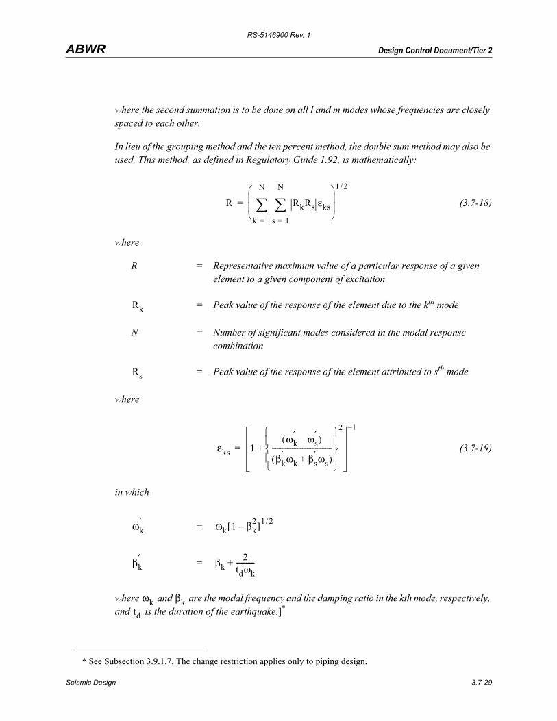
In lieu of the grouping method and the ten percent method, the double sum method may also be used. This method, as defined in Regulatory Guide 1.92, is mathematically:

(3.7-18)

where

R = Representative maximum value of a particular response of a given element to a given component of excitation

= Peak value of the response of the element due to the kth mode

N = Number of significant modes considered in the modal response combination

= Peak value of the response of the element attributed to sth mode

where

(3.7-19)

in which

=

=

where and are the modal frequency and the damping ratio in the kth mode, respectively, and is the duration of the earthquake.]*


R RkRs εks

s 1=

N

∑k 1=

N

∑⎝ ⎠⎜ ⎟⎜ ⎟⎛ ⎞ 1 2/

=

Rk

Rs

εks 1ωk

′ ωs′–( )

βk′ ωk βs

′ ωs+( )------------------------------------

⎩ ⎭⎪ ⎪⎨ ⎬⎪ ⎪⎧ ⎫2

+

1–

=

ωk′ ωk 1 βk

2–[ ]1 2/

βk′ βk

2tdωk-----------+

ωk βktd


RS-5146900 Rev. 1


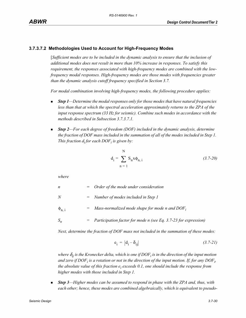
3.7.3.7.2 Methodologies Used to Account for High-Frequency Modes

[Sufficient modes are to be included in the dynamic analysis to ensure that the inclusion of additional modes does not result in more than 10% increase in responses. To satisfy this requirement, the responses associated with high-frequency modes are combined with the low-frequency modal responses. High-frequency modes are those modes with frequencies greater than the dynamic analysis cutoff frequency specified in Section 3.7.

For modal combination involving high-frequency modes, the following procedure applies:

Step 1—Determine the modal responses only for those modes that have natural frequencies less than that at which the spectral acceleration approximately returns to the ZPA of the input response spectrum (33 Hz for seismic). Combine such modes in accordance with the methods described in Subsection 3.7.3.7.1.

Step 2—For each degree of freedom (DOF) included in the dynamic analysis, determine the fraction of DOF mass included in the summation of all of the modes included in Step 1. This fraction di for each DOFi is given by:

(3.7-20)

where

n = Order of the mode under consideration

N = Number of modes included in Step 1

= Mass-normalized mode shape for mode n and DOFi

Sn = Participation factor for mode n (see Eq. 3.7-23 for expression)

Next, determine the fraction of DOF mass not included in the summation of these modes:

(3.7-21)

where δij is the Kronecker delta, which is one if DOFi is in the direction of the input motion and zero if DOFi is a rotation or not in the direction of the input motion. If, for any DOFi, the absolute value of this fraction ei exceeds 0.1, one should include the response from higher modes with those included in Step 1.

Step 3—Higher modes can be assumed to respond in phase with the ZPA and, thus, with each other; hence, these modes are combined algebraically, which is equivalent to pseudo-

di Sn

n 1=

N

∑= xφn i,

φn i,

ei di δij–=


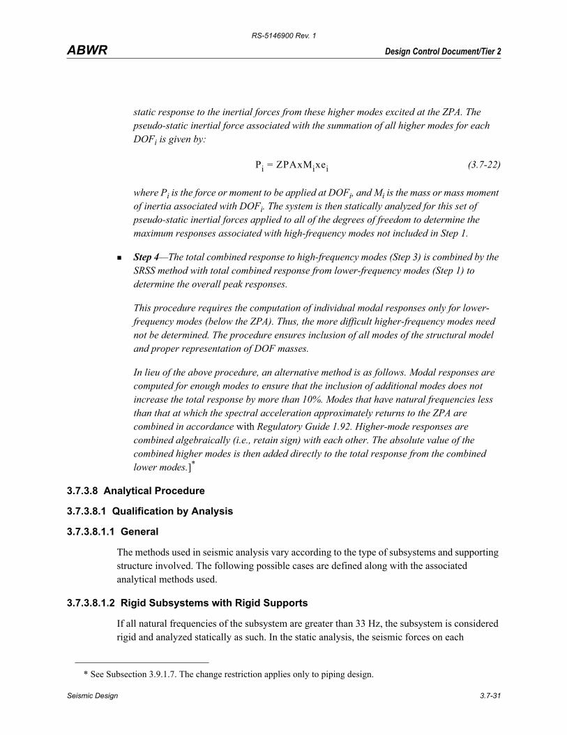
RS-5146900 Rev. 1


static response to the inertial forces from these higher modes excited at the ZPA. The pseudo-static inertial force associated with the summation of all higher modes for each DOFi is given by:

(3.7-22)

where Pi is the force or moment to be applied at DOFi, and Mi is the mass or mass moment of inertia associated with DOFi. The system is then statically analyzed for this set of pseudo-static inertial forces applied to all of the degrees of freedom to determine the maximum responses associated with high-frequency modes not included in Step 1.

Step 4—The total combined response to high-frequency modes (Step 3) is combined by the SRSS method with total combined response from lower-frequency modes (Step 1) to determine the overall peak responses.

This procedure requires the computation of individual modal responses only for lower-frequency modes (below the ZPA). Thus, the more difficult higher-frequency modes need not be determined. The procedure ensures inclusion of all modes of the structural model and proper representation of DOF masses.

In lieu of the above procedure, an alternative method is as follows. Modal responses are computed for enough modes to ensure that the inclusion of additional modes does not increase the total response by more than 10%. Modes that have natural frequencies less than that at which the spectral acceleration approximately returns to the ZPA are combined in accordance with Regulatory Guide 1.92. Higher-mode responses are combined algebraically (i.e., retain sign) with each other. The absolute value of the combined higher modes is then added directly to the total response from the combined lower modes.]*

3.7.3.8 Analytical Procedure

3.7.3.8.1 Qualification by Analysis

3.7.3.8.1.1 General

The methods used in seismic analysis vary according to the type of subsystems and supporting structure involved. The following possible cases are defined along with the associated analytical methods used.

3.7.3.8.1.2 Rigid Subsystems with Rigid Supports

If all natural frequencies of the subsystem are greater than 33 Hz, the subsystem is considered rigid and analyzed statically as such. In the static analysis, the seismic forces on each


Pi ZPA= xMixei


RS-5146900 Rev. 1


component of the subsystem are obtained by concentrating the mass at the center of gravity and multiplying the mass by the appropriate maximum floor acceleration.

3.7.3.8.1.3 Rigid Subsystems with Flexible Supports

If it can be shown that the subsystem itself is a rigid body (e.g., piping supported at only two points) while its supports are flexible, the overall subsystem is modeled as a single-degree-of-freedom subsystem consisting of an effective mass and spring.

The natural frequency of the subsystem is computed and the acceleration determined from the floor response spectrum curve using the appropriate damping value. A static analysis is performed using 1.5 times the acceleration value. In lieu of calculating the natural frequency, the peak acceleration from the spectrum curve may be used.

If the subsystem has no definite orientation, the excitation along each of three mutually perpendicular axes is aligned with respect to the system to produce maximum loading. The excitation in each of the three axes is considered to act simultaneously. The responses are combined by the SRSS method.

3.7.3.8.1.4 Flexible Subsystems

If the subsystem has more than two supports, it cannot be considered a rigid body and must be modeled as a multi-degree-of-freedom subsystem.

The subsystem is modeled as discussed in Subsection 3.7.3.3.1 in sufficient detail (i.e., number of mass points) to ensure that the lowest natural frequency between mass points is greater than 33 Hz. The mathematical model is analyzed using a time-history analysis technique or a response spectrum analysis approach. After the natural frequencies of the subsystem are obtained, a stress analysis is performed using the loads obtained from the dynamic analysis.

In a response spectrum dynamic analysis, modal responses are combined as described in Subsection 3.7.3.7. In a response spectrum or time-history dynamic analysis, responses due to the three orthogonal components of seismic excitation are combined as described is Subsection 3.7.3.6.

3.7.3.8.1.5 Static Analysis

A static analysis is performed in lieu of a dynamic analysis by applying the following forces at the concentrated mass locations (nodes) of the analytical model of the seismic subsystem:

(1) Horizontal static load, , in one of the horizontal principal directions.

(2) Equal static load, , in the other horizontal principal direction.

(3) Vertical static load, :

Fh ChW=

Fh

Fv CvW=


RS-5146900 Rev. 1


where

= Multipliers of the gravity acceleration, g, determined from the horizontal and vertical floor response spectrum curves, respectively. (They are functions of the period and the appropriate damping of the piping system)

W = Weight at node points of the analytical model

For special case analyses, and may be taken as:

(1) 1.0 times the zero-period acceleration of the response spectrum of subsystems described in Subsection 3.7.3.8.1.2.

(2) 1.5 times the value of the response spectrum at the determined frequency for subsystems described in Subsections 3.7.3.8.1.3 and 3.7.3.8.1.4.

(3) 1.5 times the peak of the response spectrum for subsystems described in Subsections 3.7.3.8.1.3 and 3.7.3.8.1.4.

An alternate method of static analysis which allows for simpler technique with added conservatism is acceptable. No determination of natural frequencies is made, but rather the response of the subsystem is assumed to be the peak of the appropriate response spectrum at a conservative and justifiable value of damping. The response is then multiplied by a static coefficient of 1.5 to take into account the effects of both multifrequency excitation and multimodal response.

3.7.3.8.1.6 Dynamic Analysis

[The dynamic analysis procedure using the response spectrum method is provided as follows:

(1) The number of node points and members is indicated. If a computer program is utilized, use the same order of number in the computer program input. The mass at each node point, the length of each member, elastic constants, and geometric properties are determined.

(2) The dynamic degrees of freedom according to the boundary conditions are determined.

(3) The dynamic properties of the subsystem (i.e., natural frequencies and mode shapes) are computed.

(4) Using a given direction of earthquake motion, the modal participation factors, , for each mode are calculated:

Ch, Cv

Ch Cv

sj


RS-5146900 Rev. 1


(3.7-23)

where

= ith mass

= Component of in the earthquake direction

= ith characteristic displacement in the jth mode

= Modal participation factor for the jth mode

N = Number of masses.

(5) Using the appropriate response spectrum curve, the spectral acceleration, , for the jth mode as a function of the jth mode natural frequency and the damping of the system is determined.

(6) The maximum modal acceleration at each mass point, i, in the model is computed as follows:

(3.7-24)

where

= Acceleration of the ith mass point in the jth mode.

(7) The maximum modal inertia force at the ith mass point for the jth mode is calculated from the equation:

(3.7-25)

(8) For each mode, the maximum inertia forces are applied to the subsystem model, and the modal forces, shears, moments, stresses, and deflections are determined.

(9) The modal forces, shears, moments, stresses, and deflections for a given direction are combined in accordance with Subsection 3.7.3.7.

sj

Miφ′ij

i 1=

N

∑

Miφij2

i 1=

N

∑

-------------------------=

Mi

φij′ φij

φij

sj

ra

aij sjrajφij=

aij

Fij Miaij=


RS-5146900 Rev. 1


(10) Steps (5) through (9) are performed for each of the three earthquake directions.

(11) The seismic force, shear, moment, and stress resulting from the simultaneous application of the three components of earthquake loading are obtained in the following manner:

(3.7-26)

R = Equivalent seismic response quantity (force, shear, moment, stress, etc.)

= Colinear response quantities due to earthquake motion in the x, y, and z directions, respectively]*

3.7.3.8.1.7 Damping Ratio

The damping ratio percentage of critical damping of subsystems corresponds to Regulatory Guide 1.61 or 1.84 (ASME Code Case N-411-1). The damping ratio is specified in Table 3.7-1.

[ASME Code Case N-411-1 damping cannot be used for analyzing linear energy absorbing supports designed in accordance with ASME Code Case N-420.]*

[Strain energy weighted modal damping can also be used in the dynamic analysis. Strain energy weighting is used to obtain the modal damping coefficient due to the contributions of elements with different damping properties in the model. The element damping values are specified in Table 3.7-1. Strain energy weighted modal damping is calculated as specified in Subsection 3.7.2.15.]†

In direct integration analysis, damping is input in the form of α and β damping constants, which give the percentage of critical damping, λ as a function of the circular frequency, ω.

(3.7-27)

3.7.3.8.1.8 Effect of Differential Building Movements

In most cases, subsystems are anchored and restrained to floors and walls of buildings that may have differential movements during a seismic event. The movements may range from insignificant differential displacements between rigid walls of a common building at low elevations to relatively large displacements between separate buildings at a high seismicity site.

* See Subsection 3.9.1.7. The change restriction applies only to piping design.† See Subsection 3.9.1.7. The change restriction applies only to piping design.

R Rx2 Ry

2 Rz2+ +=

RxRyRz

λ α2ω------- βω

2-------+=


RS-5146900 Rev. 1


Differential endpoint or restraint deflections cause forces and moments to be induced into the system. The stress thus produced is a secondary stress. It is justifiable to place this stress, which results from restraint of free-end displacement of the system, in the secondary stress category because the stresses are self-limiting and, when the stresses exceed yield strength, minor distortions or deformations within the system satisfy the condition which caused the stress to occur.

[The earthquake thus produces a stress-exhibiting property much like a thermal expansion stress and a static analysis can be used to obtain actual stresses. The differential displacements are obtained from the dynamic analysis of the building. The displacements are applied to the anchors and restraints corresponding to the maximum differential displacements which could occur. The static analysis is made three times: once for one of the horizontal differential displacements, once for the other horizontal differential displacement, and once for the vertical.

The inertia (primary) and displacement (secondary) loads are dynamic in nature and their peak values are not expected to occur at the same time. Hence, the combination of the peak values of inertia load and anchor displacement load is quite conservative. In addition, anchor movement effects are computed from static analyses in which the displacements are applied to produce the most conservative loads on the components. Therefore, the primary and secondary loads are combined by the SRSS method.]*

3.7.3.8.1.9 Design of Small Branch and Small Bore Piping

(1) [Small branch lines are defined as those lines that can be decoupled from the analytical model used for the analysis of the main run piping to which the branch lines attach. As allowed by Subsection 3.7.3.3.1.3, branch lines can be decoupled when the ratio of run to branch pipe moment of inertia is 25 to 1, or greater. In addition to the moment of inertia criterion for acceptable decoupling, these small branch lines shall be designed with no concentrated masses, such as valves, in the first one-half span length from the main run pipe; and with sufficient flexibility to prevent restraint of movement of the main run pipe. The small branch line is considered to have adequate flexibility if its first anchor or restraint to movement is at least one-half pipe span in a direction perpendicular to the direction of relative movement between the pipe run and the first anchor or restraint of the branch piping. A pipe span is defined as the length tabulated in Table NF-3611-1, Suggested Piping Support Spacing, ASME B&PV Code Section III, Subsection NF. For branches where the preceding criteria for sufficient flexibility cannot be met, the applicant will demonstrate acceptability by using an alternative criteria for sufficient flexibility, or by accounting for the effects of the branch piping in the analysis of the main run piping.


RS-5146900 Rev. 1


(2) For small bore piping defined as piping 50A and less nominal pipe size, and small branch lines 50A and less nominal pipe size, as defined in (1) above, it is acceptable to use small bore piping handbooks in lieu of performing a system flexibility analysis, using static and dynamic mathematical models, to obtain loads on the piping elements and using these loads to calculate stresses per equations in NB, NC, and ND3600 in ASME Code Section III, whenever the following are met:

(a) The small bore piping handbook at the time of application is currently accepted by the regulatory agency for use on equivalent piping at other nuclear power plants.

(b) When the small bore piping handbook is serving the purpose of the Design Report it meets all of the ASME requirements for a piping design report. This includes the piping and its supports.

(c) Formal documentation exists showing piping designed and installed to the small bore piping handbook (1) is conservative in comparison to results from a detail stress analysis for all applied loads and load combinations using static and dynamic analysis methods defined in Subsection 3.7.3, (2) does not result in piping that is less reliable because of loss of flexibility or because of excessive number of supports, (3) satisfies required clearances around sensitive components.

The small bore piping handbook methodology will not be applied when specific information is needed on (a) magnitude of pipe and fittings stresses, (b) pipe and fitting cumulative usage factors, (c) accelerations of pipe-mounted equipment, or locations of postulated breaks and leaks.

The small bore piping handbook methodology will not be applied to piping systems that are fully engineered and installed in accordance with the engineering drawings.]*

[Supports for ASME Section III instrumentation lines are analyzed in accordance with Subsection 3.7.3 and are designed in accordance with Subsection 3.9.3.4.]*

3.7.3.8.1.10 Multi–Supported Equipment and Components with Distinct Inputs

[For multi-supported systems (equipment and piping) analyzed by the response spectrum method for the determination of inertial responses, either of the following two input motions is acceptable:

(1) Envelope response spectrum of all support points for each orthogonal direction of excitation, or



RS-5146900 Rev. 1


(2) Independent support motion (ISM) response spectrum at each support for each orthogonal direction of excitation.

When the ISM response spectrum method of analysis is used, the following conditions should be met:

(1) ASME Code Case N-411-1 damping is not used.

(2) A support group is defined by supports which have the same time-history input. This usually means all supports located on the same floor, or portions of a floor, of a structure.

(3) The responses due to motions of supports in two or more different groups are combined by the SRSS procedure.

In lieu of the response spectrum analysis, the time-history method of analysis subjected to distinct support motions may be used for multi-supported systems.]*

3.7.3.8.2 Qualification by Design by Rule

For distributive systems such as cable trays, conduits, and HVAC ducts, an alternative to qualification by analysis described in Subsection 3.7.3.8.1 is the design by rule method approved by the NRC at the time of COL application.

3.7.3.9 Multi-Supported Equipment and Components with Distinct Inputs

The procedure and criteria for analysis are described in Subsections 3.7.2.1.3, 3.7.3.3.1.3, and 3.7.3.8.1.10.

3.7.3.10 Use of Constant Vertical Static Factors

All Seismic Category I subsystems and components are subjected to a vertical dynamic analysis with the vertical floor spectra or time histories defining the input. A static analysis is performed in lieu of dynamic analysis if the peak value of the applicable floor spectra times a factor of 1.5 is used in the analysis. A factor of 1.0 instead of 1.5 can be used if the equipment is simple enough such that it behaves essentially as a single degree of freedom system. If the fundamental frequency of a component in the vertical direction is greater than or equal to 33 Hz, it is treated as seismically rigid and analyzed statically using the zero period acceleration (ZPA) of the response spectrum.

3.7.3.11 Torsional Effects of Eccentric Masses

Torsional effects of eccentric masses are included for Seismic Category I subsystems similar to that for the piping systems discussed in Subsection 3.7.3.3.1.2.


RS-5146900 Rev. 1


3.7.3.12 Buried Seismic Category I Piping and Tunnels

All underground Category I buried piping systems are installed in tunnels. The following items are considered in the design and analysis:

(1) The inertial effects due to an earthquake upon tunnel systems will be adequately accounted for in the design and analysis. In case of buried tunnel systems sufficiently flexible relative to the surrounding or underlying soil, it is assumed that the systems will follow essentially the displacements and deformations that the soil would have if the systems were absent. When applicable, procedures, which take into account the phenomena of wave travel and wave reflection in compacting soil displacements from the ground displacements, are employed and the effects due to local soil settlements, soil arching, etc., are also considered in the design and analysis.

(2) The design response spectra for the underground piping are the horizontal and vertical design spectra at the ground surface given in Figures 3.7-1 and 3.7-2. These design spectra are constructed in accordance with Regulatory Guide 1.60. The piping analysis is performed using one of the methods described in Subsection 3.7.3.

(3) Since all underground Seismic Category I piping is contained in tunnels, its design, analysis and construction will be in accordance with the ASME Section III of the Boiler and Pressure Vessel Code and all sections of Tier 2 pertaining to Seismic Category I piping supports will be applied.

3.7.3.13 Interaction of Other Piping with Seismic Category I Piping

[In certain instances, non-Seismic Category I piping may be connected to Seismic Category I piping at locations other than a piece of equipment which, for purposes of analysis, could be represented as an anchor. The transition points typically occur at Seismic Category I valves which may or may not be physically anchored. Since a dynamic analysis must be modeled from pipe anchor point to anchor point, two options exist:

(1) Specify and design a structural anchor at the Seismic Category I valve and analyze the Seismic Category I subsystem;

or, if impractical to design an anchor:

(2) Analyze the subsystem from the anchor point in the Seismic Category I subsystem through the valve to either the first anchor point in the non-Seismic Category I subsystem; or for a distance such that there are at least two seismic restraints in each of the three orthogonal directions.]*



RS-5146900 Rev. 1


Where small, non-Seismic Category I piping is directly attached to Seismic Category I piping, it can be decoupled from Seismic Category I piping per Subsection 3.7.3.3.1.3.

[Furthermore, non-Seismic Category I piping (particularly high energy piping as defined in Section 3.6) is designed to withstand the SSE to avoid jeopardizing adjacent Seismic Category I piping if it is not feasible or practical to isolate these two piping systems.]*

3.7.3.14 Seismic Analysis for Reactor Internals

The modeling of RPV internals is discussed in Subsection 3.7.2.3.2. The damping values are given in Table 3.7-1. The seismic model of the RPV and internals is shown in Figure 3.7-32.

3.7.3.15 Analysis Procedures for Damping

Analysis procedures for damping are discussed in Subsections 3.7.2.15 and 3.7.3.8.1.7.

3.7.3.16 Analysis Procedure for Non-Seismic Structures in Lieu of Dynamic Analysis

For the design of non-seismic Category I structures, the procedures described in the International Building Code (IBC) seismic design criteria shall be followed.

Where a structure is required to be designed to withstand a SSE, the following limitations apply:

(1) The seismic zone shall be “Zone 3”. The seismic acceleration shall be the SSE ground acceleration.

(2) The structure shall be classified as “Essential Facility”; thereby using appropriate importance factors for wind and seismic.

(3) For dual systems (i.e., shear wall with braced steel frame), one of the two systems must be designed to be capable of carrying all of the seismic or wind loading without collapse. No credit will be given for the other for resisting lateral loads.

3.7.3.17 Methods for Seismic Analysis of Above-Ground Tanks

The seismic analysis of Category I above-ground tanks considers the following items:

(1) At least two horizontal modes of combined fluid-tank vibration and at least one vertical mode of fluid vibration are included in the analysis, taking into consideration the SSI effects as appropriate. The horizontal response analysis includes at least one impulsive mode in which the response of the tank shell and roof is coupled together with the portion of the fluid contents that move in unison with the shell, and the fundamental sloshing (convective) mode.

(2) The fundamental natural horizontal impulsive mode of vibration of the fluid-tank system is estimated giving due consideration to the flexibility of the supporting medium and to any uplifting tendencies for the tank. The rigid tank assumption is not


RS-5146900 Rev. 1


made unless it can be justified. The horizontal impulsive-mode spectral acceleration, Sa1 is then determined using this frequency and the appropriate damping for the fluid-tank system. Alternatively, the maximum spectral acceleration corresponding to the relevant damping may be used.

(3) Damping values used to determine the spectral acceleration in the impulsive mode are based upon the system damping associated with the tank shell material as well as with the soil-structure interaction (SSI).

(4) In determining the spectral acceleration in the horizontal convective mode, Sa2, the fluid damping ratio is 0.5% of critical damping unless a higher value can be substantiated by experimental results.

(5) The maximum overturning moment, Mo, at the base of the tank is obtained by the modal and spatial combination methods discussed in Subsections 3.7.3.7 and 3.7.3.6, respectively. The uplift tension resulting from Mo, is resisted either by tying the tank to the foundation with anchor bolts, etc., or by mobilizing enough fluid weight on a thickened base skirt plate. The latter method of resisting Mo, when used, must be shown to be conservative.

(6) The seismically induced hydrodynamic pressures on the tank shell at any level are determined by the modal and spatial combination methods discussed in Subsections 3.7.3.7 and 3.7.3.6 respectively. The maximum hoop forces in the tank wall are evaluated with due regard for the contribution of the vertical component of ground shaking. The beneficial effects of soil-structure interaction may be considered in this evaluation. The hydrodynamic pressure at any level is added to the hydrostatic pressure at that level to determine the hoop tension in the tank shell.

(7) Either the tank top head is located at an elevation higher than the slosh height above the top of the fluid or else is designed for pressures resulting from fluid sloshing against this head.

(8) At the point of attachment, the tank shell is designed to withstand the seismic forces imposed by the attached piping. An appropriate analysis is performed to verify this design.

(9) The tank foundation is designed to accommodate the seismic forces imposed on it. These forces include the hydrodynamic fluid pressures imposed on the base of the tank as well as the tank shell longitudinal compressive and tensile forces resulting from Mo.

(10) In addition to the above, a consideration is given to prevent buckling of tank walls and roof, failure of connecting piping, and sliding of the tank.


RS-5146900 Rev. 1


3.7.4 Seismic Instrumentation

3.7.4.1 Location and Description or Seismic Instrumentation

State-of-the-art solid-state digital instrumentation that will enable the prompt processing of the data at the plant site should be used. A triaxial time-history accelerometer should be provided at each of the following locations.

One at the finished grade in the free-field

Three in the reactor building: one located on the foundation mat at elevation –8.2m, one at floor elevation 12.3m and one at the operating floor at elevation 31.7m.

Two in the control building: one on the foundation mat at elevation –8.2m and one at elevation 7.9m.

3.7.4.2 Seismic Instrumentation Operability and Characteristics

The seismic instrumentation should operate during all modes of plant operation, including periods of plant shutdown. The maintenance and repair procedures should provide for keeping the maximum number of instruments in service during plant operation and shutdown.

The design should include provisions for inservice testing. The instruments should be capable of periodic channel checks during normal plant operation and the capability for in-place functional testing. The instrumentation on the foundation and at elevations within the same building or structure should be interconnected for common starting and common timing, and the instrumentation should contain provisions for an external remote alarm to indicate actuation. The pre-event memory of the instrumentation should be sufficient to record the onset of the earthquake. It should operate continuously during the period in which the earthquake exceeds the seismic trigger threshold and for a minimum of 5 seconds beyond the last trigger level signal. The instrument should be capable of a minimum of 25 minutes of continuous recording. The acceleration sensors should have a dynamic range of 1000:1 zero to peak (i.e. 0.00lg to 1.0g) and the frequency range should be 0.20 Hz to 50 Hz.

The seismic instrumentation system is triggered by the accelerometer signals. The actuating level should be adjustable for a minimum of 0.005g to 0.2g. The trigger is actuated whenever the acceleration exceeds 0.01g. The initial setpoint may be changed (but shall not exceed 0.02g) once sufficient plant operating data have been obtained which indicate that a different setpoint would provide better system operation.

The instrumentation should be capable of on-line digital recording all components accelerometer signals. The digitized rate of the recorder should be at least 200 samples per second, the frequency band width should be at least from 0.20 Hz to 50 Hz, and the dynamic range should be 1000:1. The instrumentation should be capable of using the recorded signal to


RS-5146900 Rev. 1


calculate the standardized cumulative absolute velocity (CAV) and the 5% of critically damped response spectrum.

The instruments should be capable of having routine channel checks, functional tests, and calibrations. The CAV shutdown threshold of 0.16g-seconds should be calibrated with the October, 1987 Whittier California earthquake record or an equivalent calibration record provided for this purpose by the manufacturer of the instrumentation. In the event that an earthquake is recorded at the plant site, all calibrations including that of the CAV will be performed to demonstrate that the system was functioning properly at the time of the earthquake.

3.7.4.3 Control Room Operator Notification

Activation of the seismic trigger causes an audible and visual annunciation in the control room to alert the plant operator that an earthquake has occurred.

3.7.4.4 Comparison of Measured and Predicted Response

Within four hours after the earthquake, the 5% damped response spectrum and the CAV for each of the three components of recorded data in the free field will be obtained and evaluated to determine if the shutdown criteria defined in EPRI reports NP-5930 (Reference 3.7-5), and NP-6695 (Reference 3.7-7) have been exceeded. The plant will be shut down when the recorded motion in the free field in any of the three directions (two horizontal and one vertical) exceeds both the response spectrum limit and the CAV limit as follows:

(1) The response spectrum limit is exceeded if:

(a) At frequencies between 2 and 10 Hz, the recorded response spectral accelerations of 5% damping exceed 0.33 of the corresponding SSE values or 0.2g, whichever is greater, or

(b) At frequencies between 1 and 2 Hz, the recorded response spectral velocity of 5% damping exceed 0.33 of the corresponding SSE values or 15.24 cm/s, whichever is greater.

(2) The CAV limit is exceeded if the CAV value calculated according to the procedures in EPRI report TR-100082 (Reference 3.7-6) is greater than 0.16 g-sec.

3.7.4.5 lnservice Surveillance

Each of the seismic instruments will be demonstrated operable by the performance of the channel check, channel calibration, and channel functional test operations. The channel checks will be performed every two weeks for the first three months of service after startup. After the initial three-month period and three consecutive successful checks, the channel checks will be performed on a monthly basis. The channel calibration will be performed during each refueling. The channel functional test will be performed every six months.


RS-5146900 Rev. 1


3.7.5 COL License Information

3.7.5.1 Seismic Design Parameters

To confirm the seismic design adequacy, the COL applicant shall demonstrate that the standardized design is applicable to the site according to the procedure specified in Subsection 2.3.1.2.

3.7.5.2 Pre-Earthquake Planning and Post-Earthquake Actions

The COL applicant shall submit to the NRC as part of its application the procedures it plans to use for pre-earthquake planning and post-earthquake actions. The procedures shall implement the seismic instrumentation program specified in Subsection 3.7.4 and follow the guidelines recommended in EPRI report NP-6695 (Reference 3.7-7), with the following exceptions:

(1) Section 3.1. Short-Term Actions

(a) Item 3. “Evaluation of Ground Motion Records”—There is a time limitation of four hours within which the licensee shall determine if the shutdown criterion has been exceeded. After an earthquake has been recorded at the site, the licensee shall provide a response spectrum calibration record and CAV calibration record to demonstrate that the system was functioning properly.

(b) Item 4. “Decision on Shutdown”—Exceedance of the EPRI criterion as amended in Subsection 3.7.4.4 of Tier 2 or observed evidence of significant damage as defined by EPRI NP-6695 shall constitute a condition for mandatory shutdown unless conditions prevent the licensee from accomplishing an orderly shutdown without jeopardizing the health and safety of the public.

(c) Add item 7. “Documentation”—The licensee shall record the chronology of events and control room problems while the earthquake evaluation is in progress.

(2) Section 4.3.1. Immediate Operator Actions. Add to the checks listed in this section a prompt check of the neutron flux monitoring instruments for stability of the reactor.

(3) Section 4.3.4. Pre-Shutdown Inspection. Exceeding the EPRI criterion or evidence of significant damage should constitute a condition for mandatory plant shutdown.

(4) Section 4.3.4.1. Safe Shutdown Equipment. In addition to the safe shutdown systems on this list, containment integrity must be maintained following an earthquake. Since the containment isolation valves may have malfunctioned during the earthquake, inspection of the containment isolation system is necessary to assure continued containment integrity.


RS-5146900 Rev. 1


3.7.5.3 Piping Analysis, Modeling of Piping Supports

The COL applicant shall provide justification for methods used other than those described in Subsection 3.7.3.3.1.6 for determining pipe support stiffness used in the piping analysis. The justification should include verification that the pipe support stiffness values are representative of the types of supports used in the piping system. The alternative approach used to determine pipe supports stiffness values and its bases should be submitted to the NRC staff for review and approval before its use (Subsection 3.7.3.3.1.6).

3.7.5.4 Assessment of Interaction Due to Seismic Effects

The COL applicant will describe the process for completion of the design of balance-of-plant and non-safety related systems to minimize II/I interactions and propose procedures for an inspection of the as-built plant for II/I interactions. (Subsection 3.7.2.8)

3.7.6 References

3.7-1 Not Used.

3.7-2 Not Used.

3.7-3 Not Used.

3.7-4 L. K. Liu, “Seismic Analysis of the Boiling Water Reactor”, symposium on seismic analysis of pressure vessel and piping components, First National Congress on Pressure Vessel and Piping, San Francisco, California, May 1971.

3.7-5 EPRI NP-5930, “A Criterion for Determining Exceedance of the Operating Basis Earthquake”, July 1988.

3.7-6 EPRI TR-100082, “Standardization of Cumulative Absolute Velocity”, December 1991.

3.7-7 EPRI NP-6695, “Guidelines for Nuclear Plant Response to an Earthquake”, December 1989.

3.7-8 P. Koss, “Seismic Testing of Electrical Cable Support Systems”, Structural Engineers of California Conference, San Diego, September 1979.


RS-5146900 Rev. 1


Table 3.7-1 Damping for Different Materials

Item

Percent Critical Damping

SSE

Reinforced concrete structures 7

Welded structural assemblies 4

Steel frame structures 4

Bolted or riveted structural assemblies 7

Equipment 3

piping systems*

* Damping values of ASME Code Case N-411-1, alternative damping values for Response Spectra Analysis of Class 1, 2, and 3 Piping, Section III, Division 1, may be used as permitted by Regulatory Guide 1.84. These damping values are applicable in analyzing piping response for Seismic and other dynamic loads filtering through building structures in high frequencies range beyond 33 Hz.

- diameter greater than 300A nominal 3

- diameter less than or equal to 300A nominal

2

Reactor pressure vessel, support skirt, shroud head and separator

4

Guide tubes and CRD housings 2

Fuel 6

Cable trays 20 (max)(see Figure 3.7-27)

Conduits 7

HVAC ductwork– companion angle– pocket lock– welded

774


RS-5146900 Rev. 1


Table 3.7-2 Natural Frequencies of the Reactor Building Complex in X Direction (0°–180° Axis)—Fixed Base Condition

Mode No. Frequency (HZ)

1 4.14

2 4.53

3 7.71

4 9.01

5 9.60

6 10.10

7 11.53

8 12.72

9 13.44

10 13.58

11 14.64

12 15.60

13 17.46

14 18.00

15 18.95

16 22.01

17 22.72

18 24.31

19 25.48

20 26.11

21 27.08

22 28.20

23 29.84

24 30.94

25 33.16


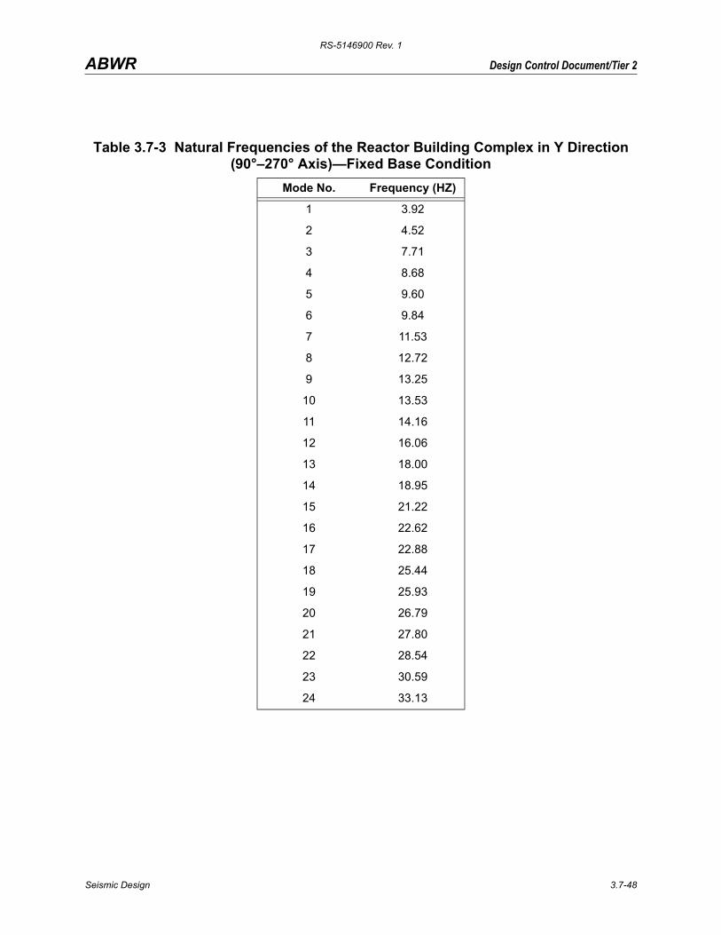
RS-5146900 Rev. 1


Table 3.7-3 Natural Frequencies of the Reactor Building Complex in Y Direction (90°–270° Axis)—Fixed Base Condition


1 3.92

2 4.52

3 7.71

4 8.68

5 9.60

6 9.84

7 11.53

8 12.72

9 13.25

10 13.53

11 14.16

12 16.06

13 18.00

14 18.95

15 21.22

16 22.62

17 22.88

18 25.44

19 25.93

20 26.79

21 27.80

22 28.54

23 30.59

24 33.13


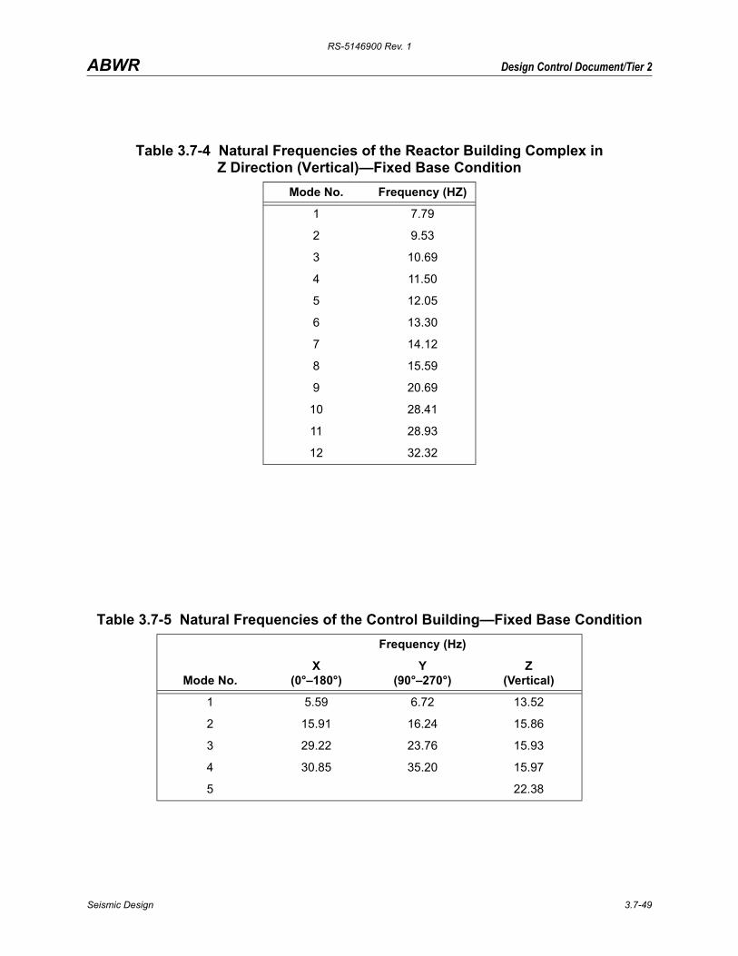
RS-5146900 Rev. 1


Table 3.7-4 Natural Frequencies of the Reactor Building Complex in Z Direction (Vertical)—Fixed Base Condition


1 7.79

2 9.53

3 10.69

4 11.50

5 12.05

6 13.30

7 14.12

8 15.59

9 20.69

10 28.41

11 28.93

12 32.32

Table 3.7-5 Natural Frequencies of the Control Building—Fixed Base ConditionFrequency (Hz)

Mode No.X

(0°–180°)Y

(90°–270°)Z

(Vertical)

1 5.59 6.72 13.52

2 15.91 16.24 15.86

3 29.22 23.76 15.93

4 30.85 35.20 15.97

5 22.38


RS-5146900 Rev. 1


Table 3.7-6 Not Used


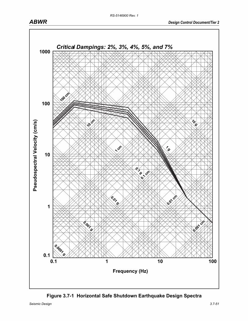
RS-5146900 Rev. 1


Figure 3.7-1 Horizontal Safe Shutdown Earthquake Design Spectra

10 g

1 g

0.1 g

0.01 g

0.001 g

0.0001 g

100 c

m

10 cm

1 cm

0.1 cm

0.01 c

m

0.001

cm

Critical Dampings: 2%, 3%, 4%, 5%, and 7%1000

100

10

1

0.10.1 1 10 100

Frequency (Hz)

Pseu

dosp

ectr

al V

eloc

ity (c

m/s

)


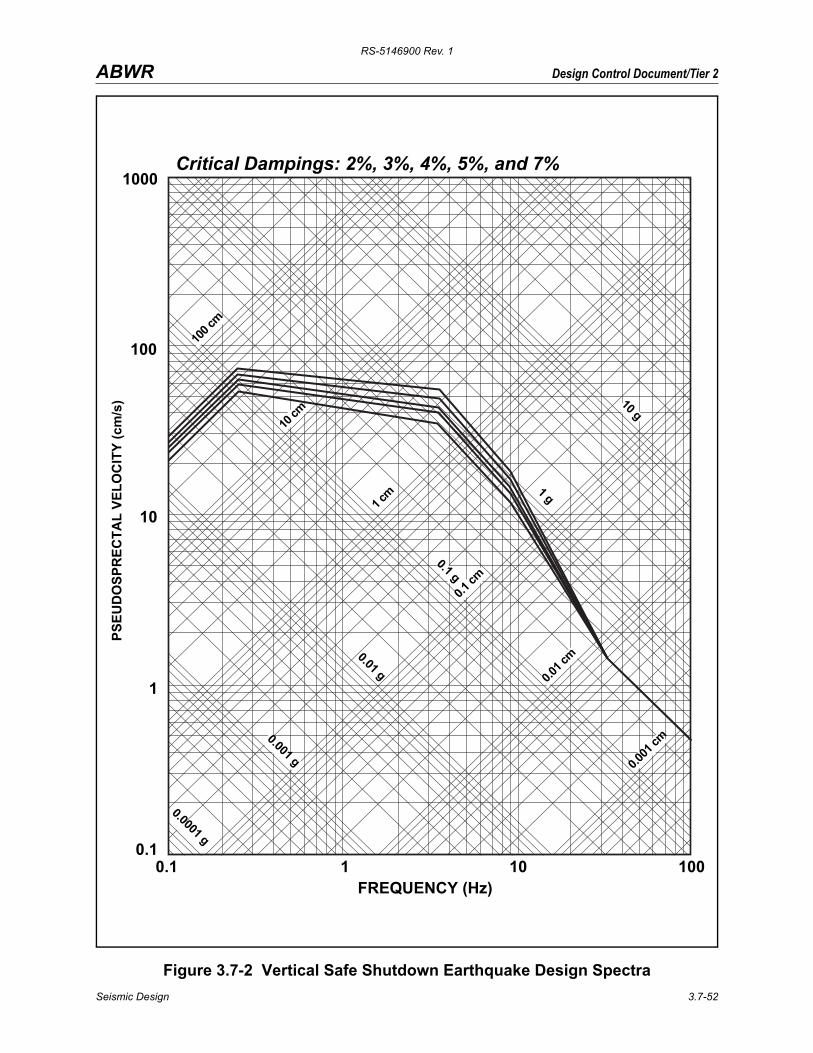
RS-5146900 Rev. 1


Figure 3.7-2 Vertical Safe Shutdown Earthquake Design Spectra

10 g

1 g

0.1 g

0.01 g

0.001 g

0.0001 g

100 c

m

10 cm

1 cm

0.1 cm

0.01 c

m

0.001

cm

Critical Dampings: 2%, 3%, 4%, 5%, and 7%1000

100

10

1

0.10.1 1 10 100

FREQUENCY (Hz)

PSEU

DO

SPR

ECTA

L VE

LOC

ITY

(cm

/s)


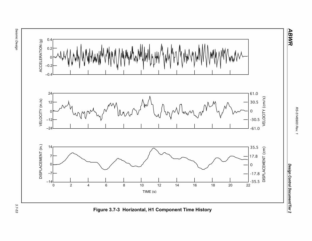
RS

-5146900 Rev. 1

Seism

ic Design

3.7-53

Design Control Document/Tier 2

ABWR

20 22

35.5

17.8

0

-17.8

-35.5 DIS

PLA

CEM

ENT (

cm)

61.0

30.5

0

-30.5

-61.0

VEL

OCIT

Y (

cm/s

)

Figure 3.7-3 Horizontal, H1 Component Time History

0.4

0.2

0

–0.2

–0.4

AC

CE

LER

ATI

ON

(g)

24

12

0

–12

–24

VE

LOC

ITY

(in.

/s)

14

7

0

–7

–14

DIS

PLA

CE

ME

NT

(in.)

0 2 4 6 8 10 12 14 16 18

TIME (s)

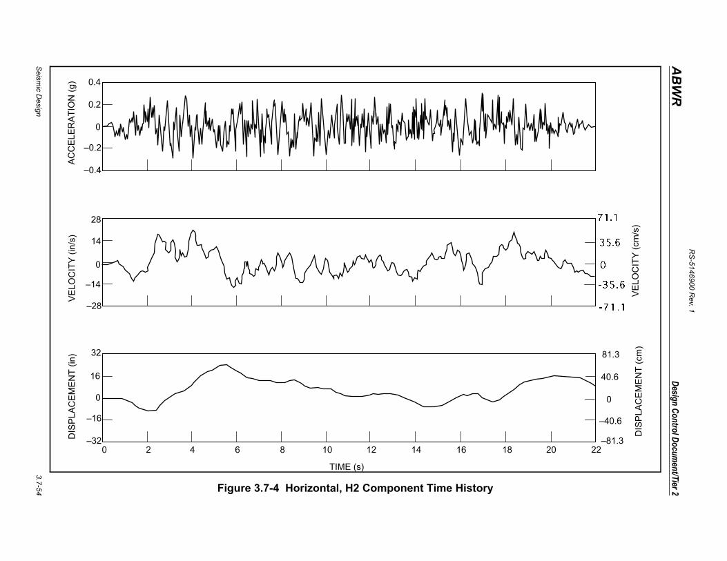
RS

-5146900 Rev. 1

Seism

ic Design

3.7-54


ABWR

8 20 22

VE

LOC

ITY

(cm

/s)

81.3

40.6

0

–40.6

–81.3

DIS

PLA

CE

ME

NT

(cm

)

Figure 3.7-4 Horizontal, H2 Component Time History

0.4

0.2

0

–0.2

–0.4

AC

CE

LER

ATI

ON

(g)

28

14

0

–14

–28

VE

LOC

ITY

(in/

s)

32

16

0

–16

–32DIS

PLA

CE

ME

NT

(in)

0 2 4 6 8 10 12 14 16 1

TIME (s)

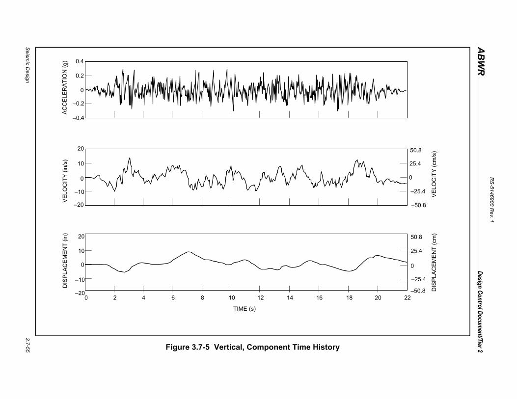
RS

-5146900 Rev. 1

Seism

ic Design

3.7-55


ABWR

20 22

VE

LOC

ITY

(cm

/s)50.8

25.4

0

–25.4

–50.8

DIS

PLA

CE

ME

NT

(cm

)

50.8

25.4

0

–25.4

–50.8

Figure 3.7-5 Vertical, Component Time History

0.4

0.2

0

–0.2

–0.4

AC

CE

LER

AT

ION

(g)

20

10

0

–10

–20

VE

LOC

ITY

(in

/s)

20

10

0

–10

–20

DIS

PLA

CE

ME

NT

(in

)

0 2 4 6 8 10 12 14 16 18

TIME (s)

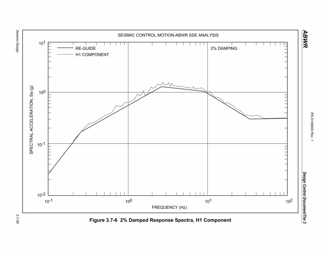
RS

-5146900 Rev. 1

Seism

ic Design

3.7-56


ABWR

t

ING

102

Figure 3.7-6 2% Damped Response Spectra, H1 Componen

101

100

10-1

10-2

10-1

FREQUENCY (Hz)

RE-GUIDE

H1 COMPONENT

2% DAMP

100 101

SEISMIC CONTROL MOTION-ABWR SSE ANALYSISS

PE

CT

RA

L A

CC

ELE

RA

TIO

N, S

a (g

)

RS

-5146900 Rev. 1

Seism

ic Design

3.7-57


ABWR

t

ING

102


101

100

10-1

10-2

10-1

FREQUENCY (Hz)

RE-GUIDE

H1 COMPONENT

3% DAMP

100 101


PE

CT

RA

L A

CC

ELE

RA

TIO

N, S

a (g

)

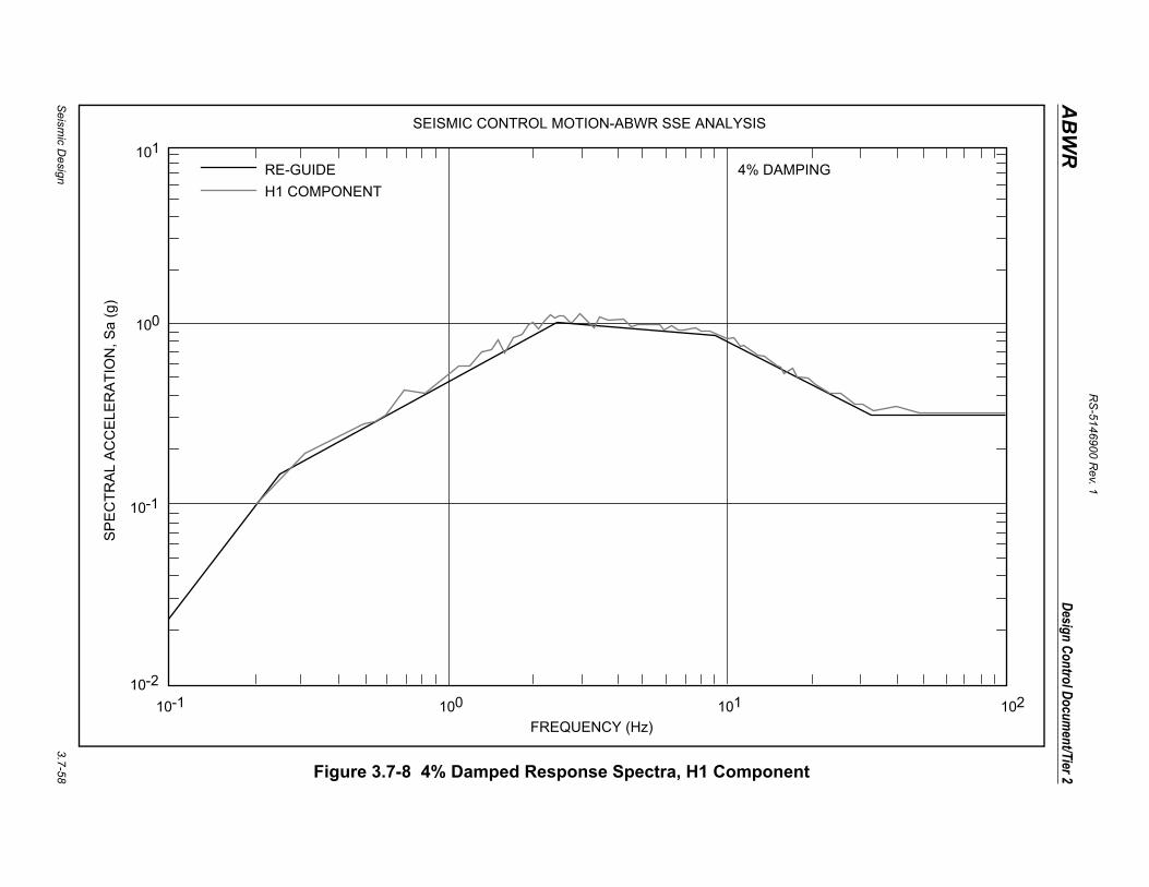
RS

-5146900 Rev. 1

Seism

ic Design

3.7-58


ABWR

t

ING

102


101

100

10-1

10-2

10-1

FREQUENCY (Hz)

RE-GUIDE

H1 COMPONENT

4% DAMP

100 101


PE

CT

RA

L A

CC

ELE

RA

TIO

N, S

a (g

)

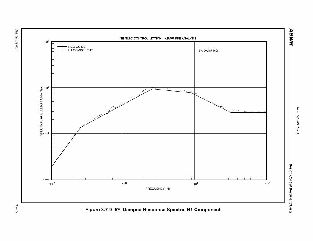
RS

-5146900 Rev. 1

Seism

ic Design

3.7-59


ABWR

t

102


FREQUENCY (Hz)

101

100

10–1

10–2

10–1 100 101

5% DAMPING

SEISMIC CONTROL MOTION – ABWR SSE ANALYSIS

REG-GUIDEH1 COMPONENT

SEISMIC CONTROL MOTION – ABWR SSE ANALYSISS

PE

CT

RA

L A

CC

ELE

RA

TIO

N –

Sa-

g

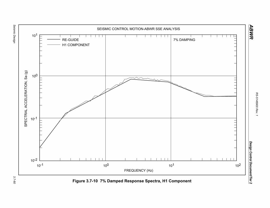
RS

-5146900 Rev. 1

Seism

ic Design

3.7-60


ABWR

nt

ING

102

Figure 3.7-10 7% Damped Response Spectra, H1 Compone

101

100

10-1

10-2

10-1

FREQUENCY (Hz)

RE-GUIDE

H1 COMPONENT

7% DAMP

100 101


PE

CT

RA

L A

CC

ELE

RA

TIO

N, S

a (g

)

RS

-5146900 Rev. 1

Seism

ic Design

3.7-61


ABWR

nt

ING

102


101

100

10-1

10-2

10-1

FREQUENCY (Hz)

RE-GUIDE

H2 COMPONENT

2% DAMP

100 101


PE

CT

RA

L A

CC

ELE

RA

TIO

N, S

a (g

)

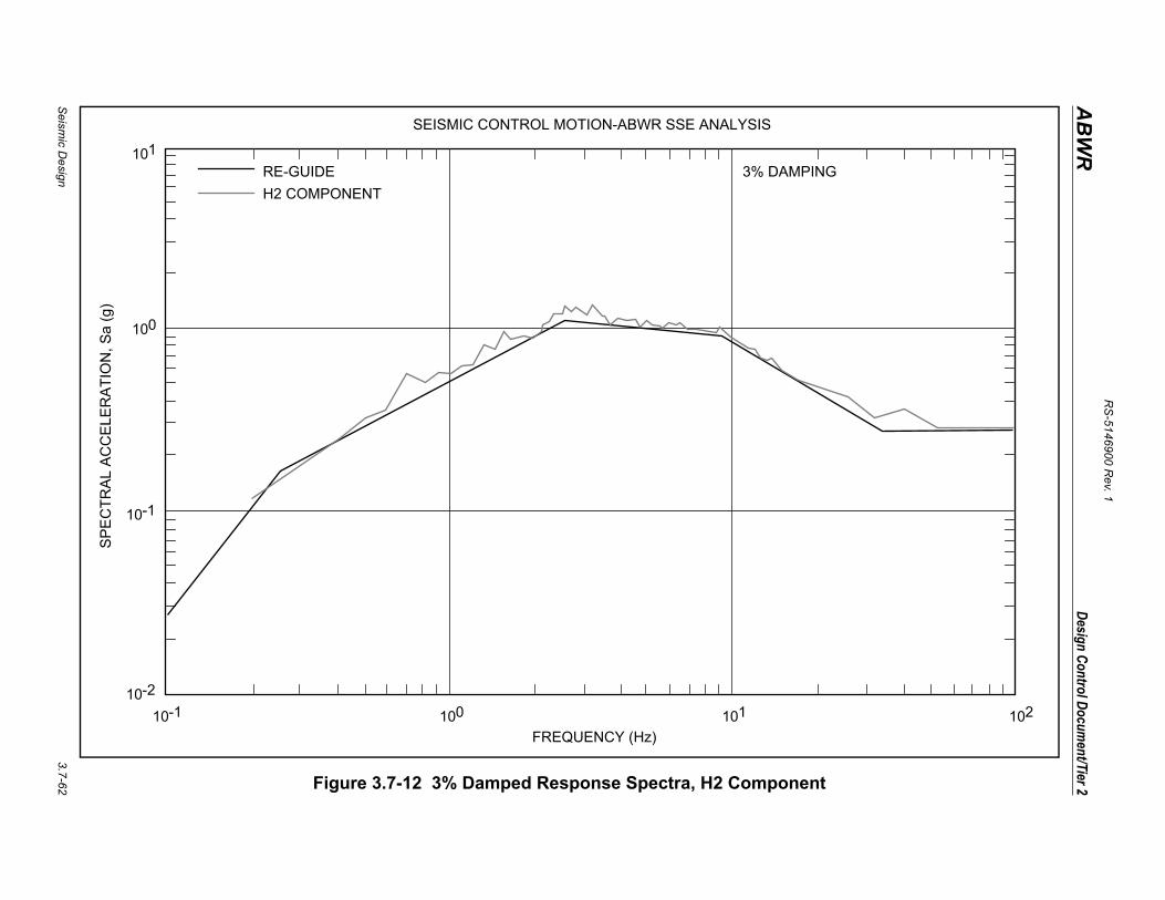
RS

-5146900 Rev. 1

Seism

ic Design

3.7-62


ABWR

nt

ING

102


101

100

10-1

10-2

10-1

FREQUENCY (Hz)

RE-GUIDE

H2 COMPONENT

3% DAMP

100 101


PE

CT

RA

L A

CC

ELE

RA

TIO

N, S

a (g

)

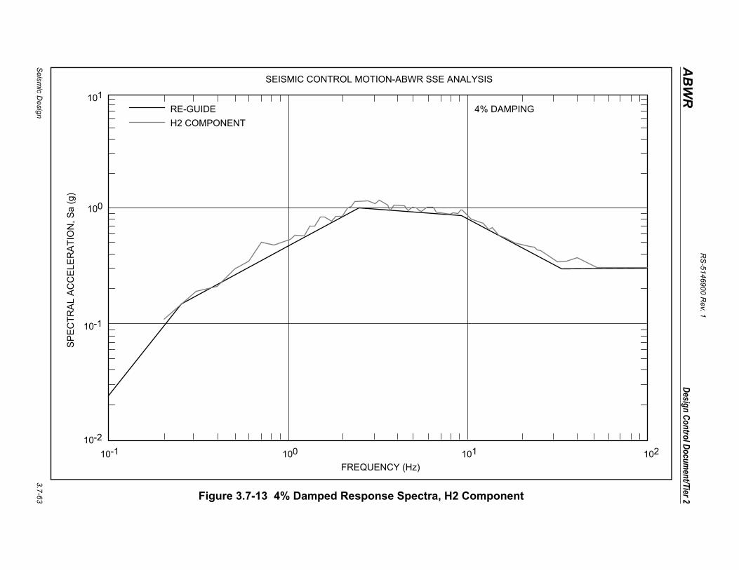
RS

-5146900 Rev. 1

Seism

ic Design

3.7-63


ABWR

nt

ING

102


101

100

10-1

10-2

10-1

FREQUENCY (Hz)

RE-GUIDE

H2 COMPONENT

4% DAMP

100 101


PE

CT

RA

L A

CC

ELE

RA

TIO

N, S

a (g

)

RS

-5146900 Rev. 1

Seism

ic Design

3.7-64


ABWR

nt

102


FREQUENCY (Hz)

SP

EC

TR

AL

AC

CE

LER

AT

ION

– S

a-g

101

100

100 101

5% DAMPING

SEISMIC CONTROL MOTION – ABWR SSE ANALYSIS

10–1

10–2

10–1

REG-GUIDEH2 COMPONENT

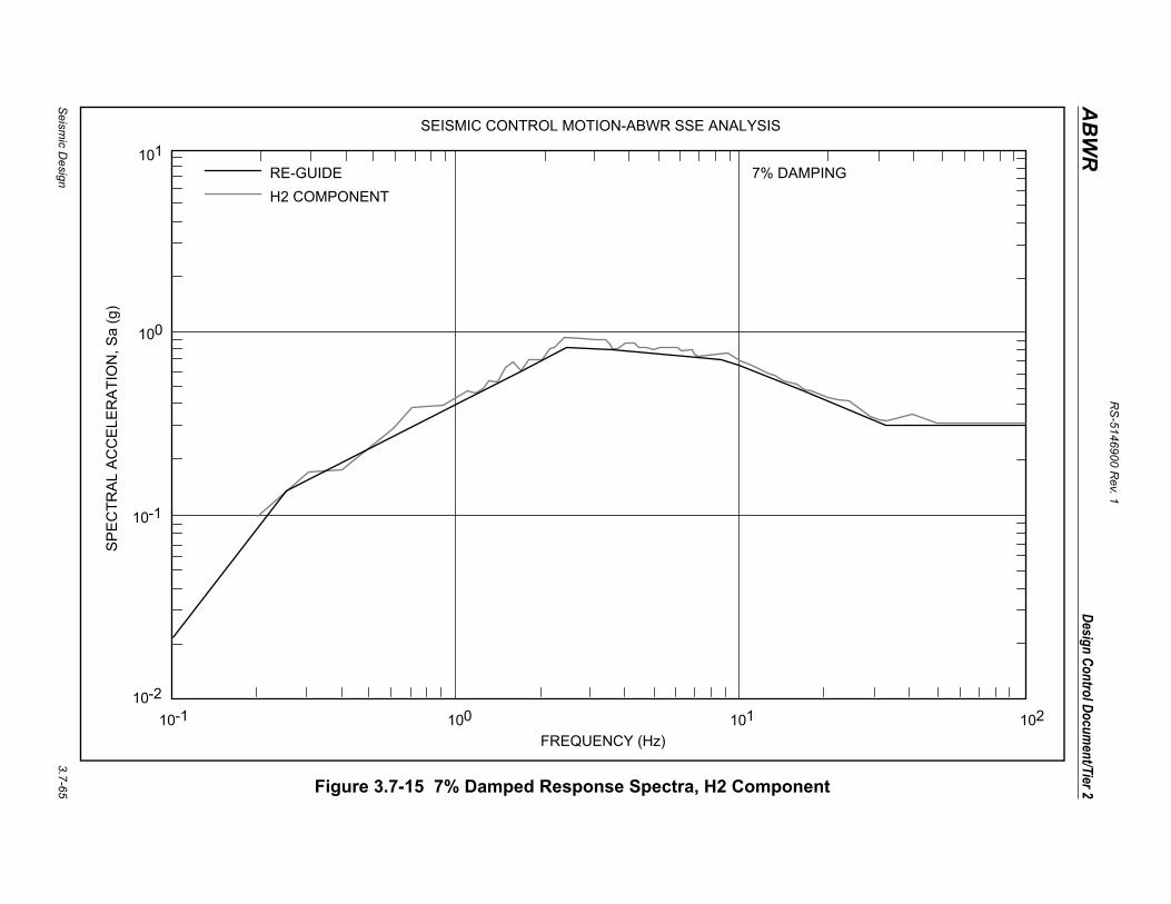
RS

-5146900 Rev. 1

Seism

ic Design

3.7-65


ABWR

nt

ING

102


101

100

10-1

10-2

10-1

FREQUENCY (Hz)

RE-GUIDE 7% DAMP

100 101


PE

CT

RA

L A

CC

ELE

RA

TIO

N, S

a (g

)

H2 COMPONENT

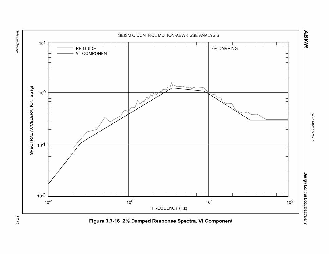
RS

-5146900 Rev. 1

Seism

ic Design

3.7-66


ABWR

t

ING

102

Figure 3.7-16 2% Damped Response Spectra, Vt Componen

101

100

10-1

10-2

10-1

FREQUENCY (Hz)

RE-GUIDEVT COMPONENT

2% DAMP

100 101


PE

CT

RA

L A

CC

ELE

RA

TIO

N, S

a (g

)

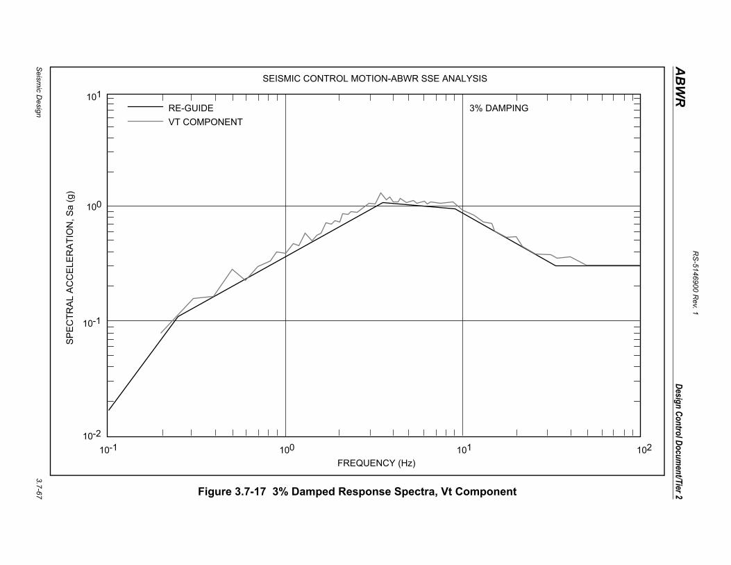
RS

-5146900 Rev. 1

Seism

ic Design

3.7-67


ABWR

t

ING

102


101

100

10-1

10-2

10-1

FREQUENCY (Hz)

RE-GUIDE

VT COMPONENT

3% DAMP

100 101


PE

CT

RA

L A

CC

ELE

RA

TIO

N, S

a (g

)

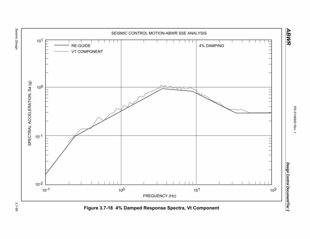
RS

-5146900 Rev. 1

Seism

ic Design

3.7-68


ABWR

t

ING

102


101

100

10-1

10-2

10-1

FREQUENCY (Hz)

RE-GUIDE

VT COMPONENT

4% DAMP

100 101


PE

CT

RA

L A

CC

ELE

RA

TIO

N, S

a (g

)

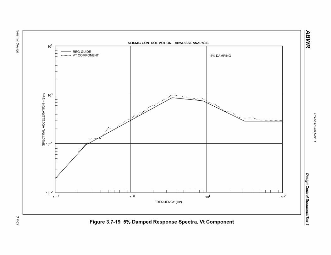
RS

-5146900 Rev. 1

Seism

ic Design

3.7-69


ABWR

t

102


FREQUENCY (Hz)

101

100

100 101

5% DAMPING

SEISMIC CONTROL MOTION – ABWR SSE ANALYSISSEISMIC CONTROL MOTION – ABWR SSE ANALYSISS

PE

CT

RA

L A

CC

ELE

RA

TIO

N –

Sa-

g

10–1

10–2

10–1

REG-GUIDEVT COMPONENT

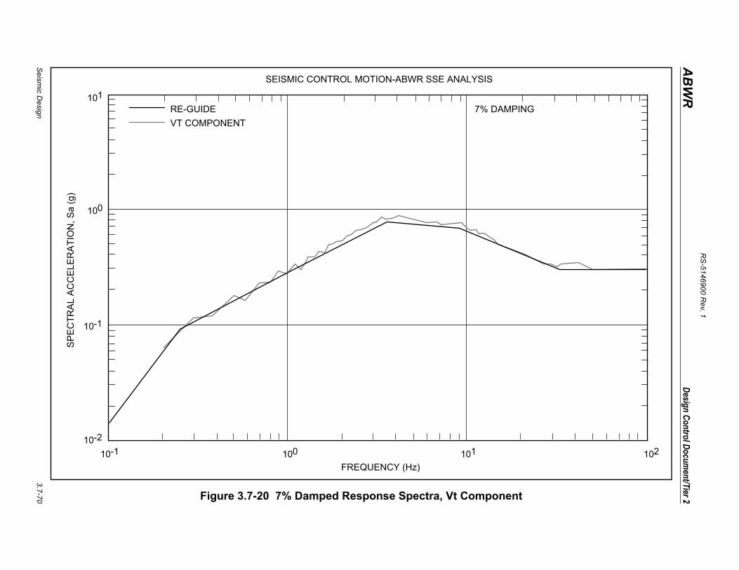
RS

-5146900 Rev. 1

Seism

ic Design

3.7-70


ABWR

t

ING

102


101

100

10-1

10-2

10-1

FREQUENCY (Hz)

RE-GUIDE

VT COMPONENT

7% DAMP

100 101


PE

CT

RA

L A

CC

ELE

RA

TIO

N, S

a (g

)

RS-5146900 Rev. 1


Figure 3.7-21 Not Used




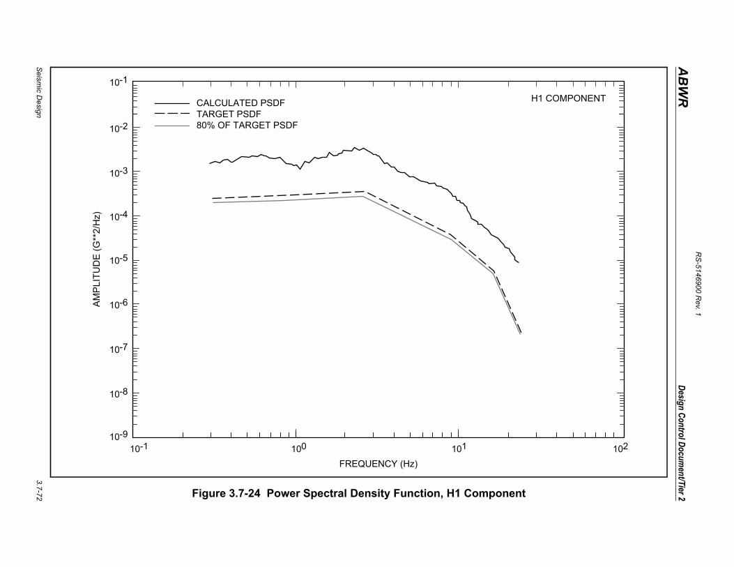
RS

-5146900 Rev. 1

Seism

ic Design

3.7-72


ABWR

ent

102

H1 COMPONENT

Figure 3.7-24 Power Spectral Density Function, H1 Compon

10-1

10-2

10-3

10-4

10-5

10-6

10-7

10-8

10-9

AM

PLI

TU

DE

(G

**2/

Hz)

10-1 100 101

FREQUENCY (Hz)

CALCULATED PSDFTARGET PSDF80% OF TARGET PSDF

RS

-5146900 Rev. 1

Seism

ic Design

3.7-73


ABWR

ent

102

H2 COMPONENT

Figure 3.7-25 Power Spectral Density Function, H2 Compon

10-1

10-2

10-3

10-4

10-5

10-6

10-7

10-8

10-9

AM

PLI

TU

DE

(G

**2/

Hz)

10-1 100 101

FREQUENCY (Hz)

CALCULATED PSDFTARGET PSDF80% OF TARGET PSDF

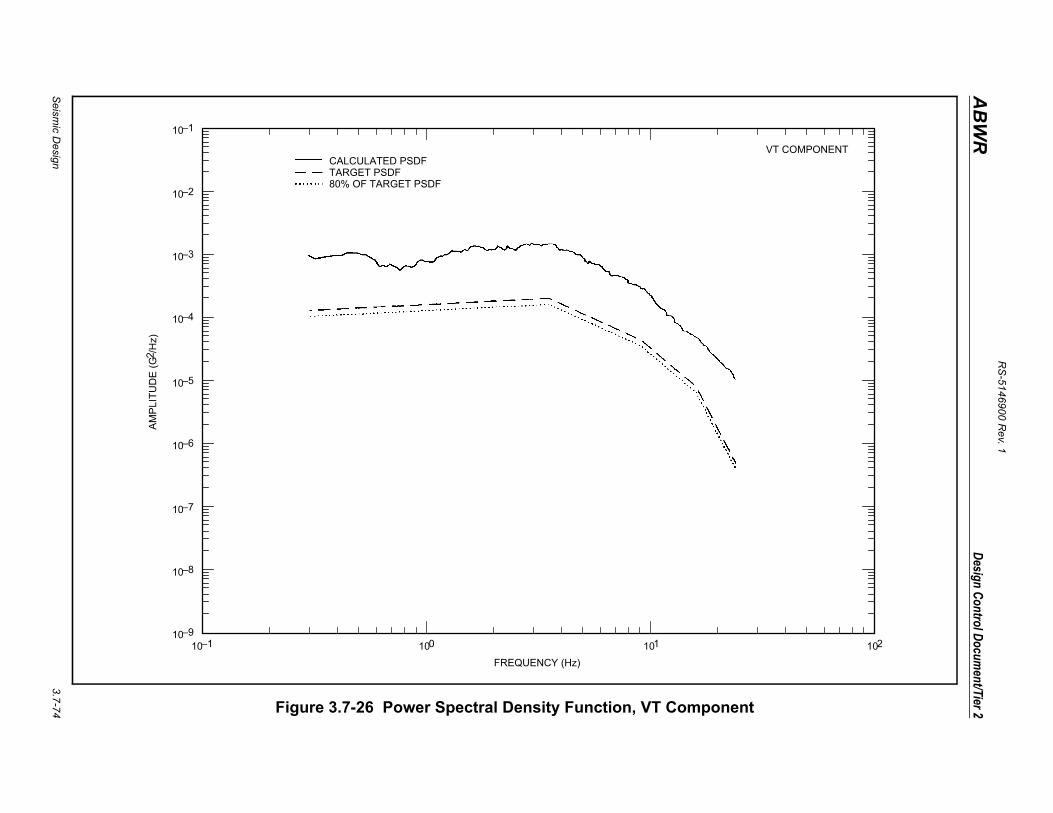
RS

-5146900 Rev. 1

Seism

ic Design

3.7-74


ABWR

ent

102

VT COMPONENT

Figure 3.7-26 Power Spectral Density Function, VT Compon

10–1

10–2

10–3

10–4

10–5

10–6

10–7

10–8

10–910–1 100 101

FREQUENCY (Hz)

AM

PLI

TUD

E (G

2 /H

z)CALCULATED PSDFTARGET PSDF80% OF TARGET PSDF

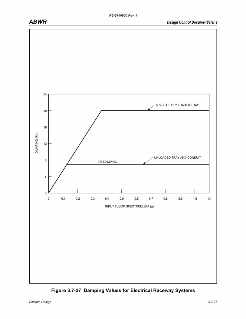
RS-5146900 Rev. 1


Figure 3.7-27 Damping Values for Electrical Raceway Systems

24

20

16

12

8

4

0

0 0.1 0.2 0.3 0.4 0.5 0.6 0.7 0.8 0.9 1.0 1.1

INPUT FLOOR SPECTRUM ZPA (g)

DA

MP

ING

(%

)

50% TO FULLY LOADED TRAY

UNLOADED TRAY AND CONDUIT7% DAMPING


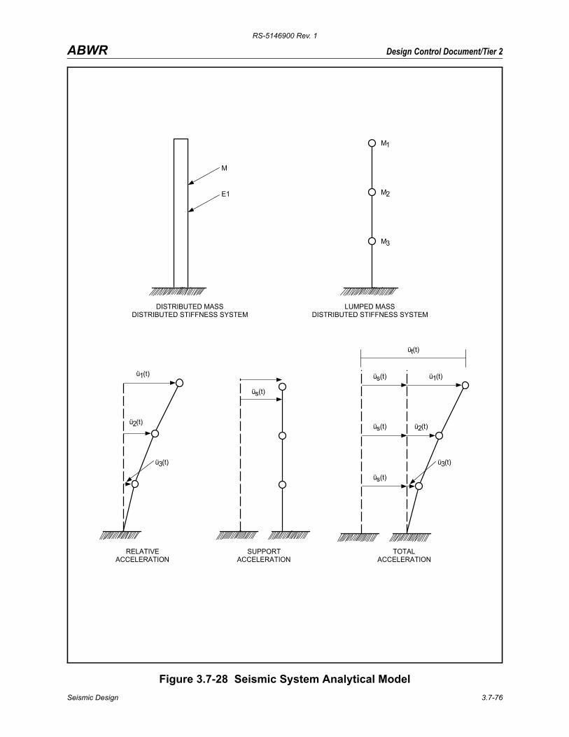
RS-5146900 Rev. 1


Figure 3.7-28 Seismic System Analytical Model

M

E1

DISTRIBUTED MASSDISTRIBUTED STIFFNESS SYSTEM

M1

M2

M3

LUMPED MASSDISTRIBUTED STIFFNESS SYSTEM

ü1(t)

ü2(t)

ü3(t)

RELATIVEACCELERATION

üs(t)

SUPPORTACCELERATION

ü3(t)

üs(t)

üs(t)

üs(t)

üt(t)

ü2(t)

ü1(t)

TOTALACCELERATION


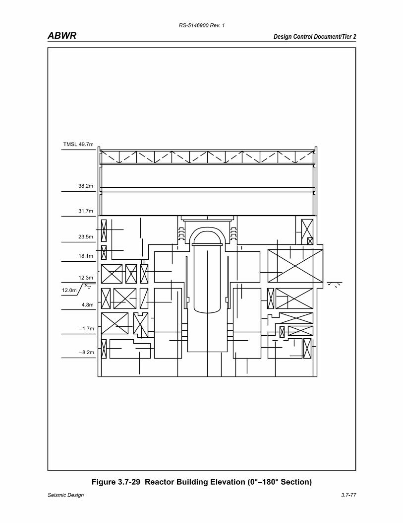
RS-5146900 Rev. 1


Figure 3.7-29 Reactor Building Elevation (0°–180° Section)

TMSL 49.7m

38.2m

31.7m

18.1m

23.5m

12.3m

12.0m

4.8m

– 1.7m

– 8.2m


RS-5146900 Rev. 1


Figure 3.7-30 Reactor Building Elevation (90°–270° Section)

TMSL 49.7m

38.2m

31.7m

18.1m

23.5m

12.3m

12.0m

4.8m

– 1.7m

– 8.2m


RS-5146900 Rev. 1


Figure 3.7-31 Reactor Building Model (see Figure 3A-8)

Figure 3.7-32 Reactor Pressure Vessel (RPV) and Internals Model (see Figure 3A-9)

Figure 3.7-33 Control Building Dynamic Model (see Figure 3A-27)


RS-5146900 Rev. 1




Toshiba Design Control Document Rev. 1 - Tier 2 - S

Documents