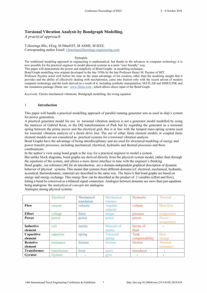
Torsional Vibration Analysis by Bondgraph Modelling. A ...

Torsional Vibration Analysis by Bondgraph Modelling. A practical approach

T.Heeringa BSc, EEng, M IMarEST, M ASME, M IEEE.Corresponding author Email: [email protected]

Synopsis The traditional modeling approach in engineering is mathematical, but thanks to the advances in computer technology it is now possible for the practical engineer to model physical systems in a more “user friendly” way. This paper will demonstrate the power and simplicity of Bond Graphs in modelling technique. Bond Graph modelling was original developed in the late 1950s by the late Professor Henry M. Paynter of MIT. Professor Paynter acted well before his time as the main advantage of his creation, other than the modeling insight that it provides and the ability of effectively dealing with mechatronics, came into fruition only with the recent advent of modern computer technology and the tools derived as a result of it, including symbolic manipulation, MATLAB and SIMULINK and the simulation package 20sim, see: www.20sim.com , which allows direct input of the Bond Graph.

Keywords: Electro-mechanical vibrations, Bondgraph modelling, the swing equation

1 Introduction

This paper will handle a practical modelling approach of parallel running generator sets as used in ship’s system for power generation. A practical generator model for use in torsional vibration analysis is not a generator model modelled by using the matrices of Gabriel Kron, or the DQ transformation of Park but by regarding the generator as a torsional spring between the prime mover and the electrical grid, this is in line with the lumped mass-spring system used for torsional vibration analysis of a diesel drive line. The use of either finite element models or coupled finite element models are not considered as practical systems for a torsional vibration analysis. Bond Graphs have the advantage of being interdisciplinary and are used for structured modeling of energy and power transfer processes, including mechanical, electrical, hydraulic and thermal processes and there combinations. In the author’s view using bond graph is the way for a practical engineer to model a system. But unlike block diagrams, bond graphs are derived directly from the physical system model, rather than through the equations of the system, and allows a more direct interface in tune with the engineer’s thinking. Bond graphs , see reference [40] for an introduction, are a domain-independent graphical description of dynamic behavior of physical systems. This means that systems from different domains (cf. electrical, mechanical, hydraulic, acoustical, thermodynamic, material) are described in the same way. The basis is that bond graphs are based on energy and energy exchange. This energy flow can be described as the product of 2 variables (effort and flow), letting a bond be conceived as a bilateral signal connection. Analogies between domains are more than just equations being analogous: the used physical concepts are analogous. Analogies among physical systems:

Electrical Mechanical translation

Mechanical rotation

Hydraulic Thermal

Flow current velocity Angular velocity

volume Heat flow

Effort voltage force torque pressure temperature Power power power power power Power ·

temperature Inductive element

coil inertia Moment of inertia

Inertia of fluid

-

Capacitive element

capacitor spring Torsional spring

Tank, compressibility

Heat storage

Resistive element

resistance friction friction friction Thermal resistance

Transformer transformer lever gears transducer - Gyrator Gyrator - gyro - -

Conference Proceedings of INEC 2 – 4 October 2018

14th International Naval Engineering Conference & Exhibition 1 http://doi.org/10.24868/issn.2515-818X.2018.034

Bond-graph modelling is a powerful tool for modelling engineering systems, especially when different physical domains are involved. Furthermore, bond-graph submodels can be re-used elegantly, because bond-graph models are non-causal. The submodels can be seen as objects; bond-graph modelling is a form of object-oriented physical systems modelling.

Bond graphs are labelled and directed graphs, in which the vertices represent submodels and the edges represent an ideal energy connection between power ports. The vertices are idealized descriptions of physical phenomena: they are concepts, denoting the relevant (i.e. dominant and interesting) aspects of the dynamic behavior of the system. It can be bond graphs itself, thus allowing hierarchical models, or it can be a set of equations in the variables of the ports (two at each port). The edges are called bonds. They denote point-to-point connections between submodel ports. When preparing for simulation, the bonds are embodied as two-signal connections with opposite directions. Furthermore, a bond has a power direction and a computational causality direction. Proper assigning the power direction resolves the sign-placing problem when connecting submodels structures. The internals of the submodels give preferences to the computational direction of the bonds to be connected. The eventually assigned computational causality dictates which port variable will be computed as a result (output) and consequently, the other port variable will be the cause (input). Therefore, it is necessary to rewrite equations if another computational form is specified then is needed. Since bond graphs can be mixed with block-diagram parts, bond-graph submodels can have power ports, signal inputs and signal outputs as their interfacing elements. Furthermore, aspects like the physical domain of a bond (energy flow) can be used to support the modelling process.

The concept of bond graphs was originated by Paynter (1961). The idea was further developed by Karnopp and Rosenberg in their textbooks (1968, 1975, 1983, 1990), such that it could be used in practice (Thoma, 1975; Van Dixhoorn, 1982). By means of the formulation by Breedveld (1984, 1985) of a framework based on thermodynamics, bond-graph model description evolved to a systems theory.

For a more thoroughly analysis of bond graphs the author refer to the extensive amount of literature available see among others the reference list: [1], [4], [5], [6], [9], [10], [12], [13], [14], [15], [16], [17], [19], [20]. Reference [40] and [42] gives a very good introduction in the use of bond graphs. [41] is an example how to use bond graphs in electronics.For Matlab users there is Bond graph add-on block library BG V2.1. see www.mathworks.com

As an introduction to the synchronous generator model the swing equation will be handled for a justification to consider the generator as a mass coupled with a torsional spring to the grid inertia. Another reason for a detailed explanation of the swing equation is because a literature review revealed that this important property of a synchronous generator is not get the required attendance in the author’s view. Another reason for this paper there is not much literature handling the weak grids on board of ship’s and the author’s involvement solving a power oscillation problem in a ship’s power plant, see the oscillation in the figures 11, 12 and 13. Also a practical diesel model with the dynamics of the governor and the fuel pump delay for TVA purpose will be presented. The model parameters as internal friction and damping are validated from torque measurements on a 12 cylinder generatorset engine but because of a NDA agreement the author was not allowed to use the data of that interesting project. The flexible coupling between the prime mover and the generator will also reviewed, it appears to be a highly nonlinear piece of equipment.



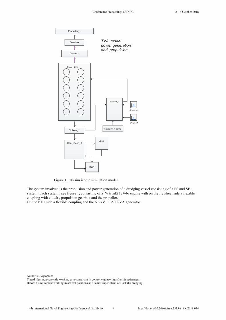
Figure 1. 20-sim iconic simulation model.

The system involved is the propulsion and power generation of a dredging vessel consisting of a PS and SB system. Each system , see figure 1, consisting of a Wärtsilä 12V46 engine with on the flywheel side a flexible coupling with clutch , propulsion gearbox and the propeller. On the PTO side a flexible coupling and the 6.6 kV 11350 KVA generator.

Author’s Biographies Tjeerd Heeringa currently working as a consultant in control engineering after his retirement. Before his retirement working in several positions as a senior superintend of Boskalis dredging

TVA model power generation and propulsion.

Clutch_1

Diesel_12V46

Droop_off

Droop_on

Gearbox

Gen_mech_1

Governor_1

Grid

KW1

Propeller_1

setpoint_speedVulkan_1



2 Introduction to the swing equation

As mentioned in the introduction in most text books this subject is not very clearly explained therefore we will pay some more attention on this important subject. Almost all energy consumed by various loads in an electric power system is produced by synchronous machines, or more correctly, the conversion from the primary energy sources, like water energy, nuclear energy, diesel engines, or chemical energy, to electrical energy is done in synchronous machines

2.1 Introduction

The tendency of a power system to develop restoring forces equal to or greater than the disturbing forces to maintain the state of equilibrium is known as stability If the forces tending to hold the state of equilibrium with one other are sufficient to overcome the disturbing forces, the system is said to remain stable (to stay in synchronism).

2.2 Oscillations

The combination of an inertial and an elastic restoring torque makes possible the generation of oscillations by reason of the interchange of energy between the two. Oscillatory conditions may arise in several ways, especially where there are forced vibrations near to that of the natural frequency. Oscillation amplitudes may substantially increase by mechanical torque pulsating at low frequency , as in a generator driven by a diesel engine. In ship propulsion with direct electric drive , fluctuating load torque may by impressed by the screws. Rope elasticity in the vertical or inclined haulage of mine winders may resonate with the load mass at a frequency near to the natural frequency of the machine or of its closed-loop control drives. Induction and synchronous machines respond in different ways to a change of load. The induction machine responds by a change of slip, and therefore of speed, and oscillations are of purely mechanical origin The synchronous machines, when operating in parallel with other synchronous machines or on supply bus bars, respond by adjusting its torque angle without change in mean speed: any divergence between actual and equilibrium angles calls into play a synchronizing torque proportional to a function of the angle of divergence and so adding to the system an elastic torque of electrical origin. More general the synchronous machine as an energy converter and the coupling between the mechanical drive and the electrical grid, behaves like a torsional spring with damping. A case of interest is that when the load change is cyclic.

2.3 Cyclic disturbing torque.

Cyclic irregularity in the driving torque of a generator (as when it is driven by a diesel engine), or in the load torque of a motor (as for an air compressor drive), or in a control system ( e.g. governor ‘hunting’) excite small fluctuations in speed. See reference [35]. With induction motors the speed variations are constrained by the system inertia and the inherent damping by 𝐼"𝑅 loss is large. With synchronous machines the synchronizing torque adds electrical elasticity and provides a combination with a natural oscillation frequency. If this is close to the frequency of the cyclic disturbance and if the damping is small the conditions may be such as to result in considerable phase-swing.

2.4 The generator.

The synchronous generator can be described by various mathematical models which have arisen from different methods of approach in the course of the development of the theory of electrical machines. Depending on the task, the following methods are most frequently chosen;

Park’s system of equations, see reference [27].



Model based on the rotating-field theory, Treatment as an asynchronous machine with distributed damper winding, Representation as a synchronous machine with distributed damper winding. The above mentioned descriptions are not easily suitable for use in torsional vibration calculations. We want to have a generator model which is in line with the used mass-rotating spring system or lumped mass-spring system of the diesel. Looking at energy level a generator can be viewed as rotating transformer, it transforms rotating mechanical energy by means of a rotating magnetic field in electrical energy.

Under normal operating conditions, the relative position of the rotor axis and the resultant rotor magnetic field is fixed. The angle between the two is known as the power angle or torque angle. During any disturbance, for instance the unequal angle of rotation of the driving shaft of a diesel engine, the rotor will decelerate or accelerate with respect to the synchronously rotating air gap mmf, and a relative motion begins. The equation describing this relative motion is known as the swing equation.

In addition to the state-space representation and model analysis, we will use the block diagram representation and torque-angle relationship to analyze the system stability. While this approach is not suited for a detailed study of large systems it is useful in gaining physical insight and it fits in the mass-spring system approach of the mechanical torsional vibration calculations. And it fits very well in system modeling by Bondgraph’s which is an elegant tool for total system modeling. A diesel generator set is a mechanical-electrical system and two or more generator set’s running parallel form a mechanical – electrical system, magnetically coupled. As an introduction to the theory of the generator rotor dynamics, “the swing equation”, a brief description of electrical power generating systems will be given.

2.5 Electrical power generating systems.

1) A turbine driven electrical power generating system

Figure 1. Turbo generator set. ( copy from ref.[7] page 142, figure 5.1 )

Generating unit as an oscillating system: (a) division of the rotor mass into individual sections; (b) schematic diagram; (c) torsional displacements. When the circuit breaker (in the red circle) is closed the right hand side of Figure 1 is valid, the grid inertia is coupled by a magnetic spring to the rotor inertia.

HP = high pressure turbine section IP = intermediate pressure turbine section LP = low pressure turbine section G = Generator



Ex = rotating exciter = stiffness shaft or coupling = angular displacement of a mass = external torque acting on a mass = moment of inertia of individual sections

Figure 2 Turbine unit as an oscillating system when coupled to the electrical system.

As the stiffness of the shafts and couplings is much higher than the stiffness of the “magnetic spring” the system simplifies to a two masses one spring system. See figure 2: 𝐼$= combined inertia turbo generator 𝐼"= inertia electrical system 𝐷'= magnetic damping turbo generator 𝐾'= magnetic elasticity turbo generator Both magnetic parameters 𝐷' and 𝐾' are dependent of the generator load. Simulations revealed that the damping is also influenced by the grid inertia, in today’s ship’s systems with VFD as propulsion drive the inertia of the propulsion motor is decoupled from the ship’s grid.

2) A diesel driven electrical power generating system.

Figure 3. Diesel driven generator set.

The prime mover in this system is a diesel engine and because the unequal angle of rotation of a diesel engine (see reference [10]) a flexible coupling is needed between the diesel and the synchronous generator. As the turbine has an equal angle of rotation the coupling between the turbine and the generator is a stiff one so, the inertia of the turbine can be combined with the inertia of the generator. With a diesel as a prime mover for the generator this simplification is not allowed. The simplification in this case is that the shaft stiffness is much higher than then stiffness of the coupling so the system of Fig. 3 is a two masses one spring system.

Figure 4 Generating unit from Fig. 3 as an oscillating system.

𝐼$ = inertia crankshaft + flywheel 𝐼" = inertia generator 𝐾$ = stiffness flexible coupling

According reference [2] the resonance frequency of this system is:

kdtJ

mD mK1I2I

Inertiaprimemover

Inertiagenerator

1I 2I1K



𝜔+ = ,𝐾 ∙ ./0.1./∙.1 (1)

When the diesel crankshaft has a torsional vibration damper on the non-driven side the simplified system is like this:

Figure 5. Generating unit as an oscillating system:

𝐼$ = damper 𝐼" = inertia crankshaft + flywheel 𝐼2 = inertia generator 𝐾$ = stiffness torsional damper 𝐾" = stiffness flexible coupling

The resonance frequencies of this system (Figure 5) can still be calculated by a pocket calculator again according reference [2], see the formulae below. This can be useful for a quick check of the simulation output.

𝜔+/,1 = 40.5 ∙ 𝐴 ∓ 0.5√𝐴" − 4𝐵 (2)

𝐴 = >/./+ >1

.@+ >/0>1

.1𝐵 = >/×>1

./×.1×.@∙ (𝐼$ + 𝐼" + 𝐼2)

When the diesel generator set is coupled to the electrical system than the oscillating system becomes complex as depicted in Figure 6.

Figure 6 The rotor inertia 𝐼2 is coupled magnetically to the “inertia” of the electrical system.

𝐼$ = damper on the NDE of the crankshaft 𝐼" = inertia crankshaft + flywheel 𝐼2 = inertia generator 𝐾$ = stiffness torsional damper 𝐾" = stiffness flexible coupling 𝐾' = stiffness magnetic “spring” 𝐷' = magnetic damping

3 The Swing equation

The equation governing the motion of the rotor of a synchronous machine is based on the elementary principle in dynamics which states that accelerating torque is the product of the momentum of inertia of the rotor times its angular acceleration. In the MKS system of units, this equation can be written for the synchronous generator in the form:

1I 2I 3I1K 2K

1K 2K1I 2I 3I mD mK



𝐽 ∙ E1FGEH1

+ 𝐷E ∙ 𝜔' = 𝑇J = 𝑇' − 𝑇K [N.m] (3)

where the symbols have the following meanings:

𝐽 the total moment of inertia of the rotor ( kg.m2) 𝐷E the damping-torque coefficient (Nms) 𝜔' the rotor shaft velocity (mechanical rad/s.). 𝜔L the synchronous speed. 𝑡 time, in seconds. 𝑇' the mechanical or shaft torque supplied by the prime mover, in Nm. 𝑇K the net electrical or electromagnetic torque, in Nm. 𝑇J the net accelerating torque, in Nm.

In the steady-state the rotor angular speed is synchronous speed 𝜔L' whilst the torque 𝑇N is equal to the sum of the electromagnetic torque 𝑇K and the damping (or rotational loss) torque 𝐷E ∙ 𝜔L'

𝑇H = 𝑇K + 𝐷E ∙ 𝜔L' or 𝑇' = 𝑇H − 𝐷E ∙ 𝜔L' = 𝑇K (4)

where 𝑇' is the net mechanical shaft torque i.e. the diesel torque less the rotational losses at 𝜔' = 𝜔L'. It is this torque that is converted into electromagnetic torque. If, due to some disturbance, 𝑇' > 𝑇K then it accelerates, if 𝑇' <𝑇K then it decelerates.

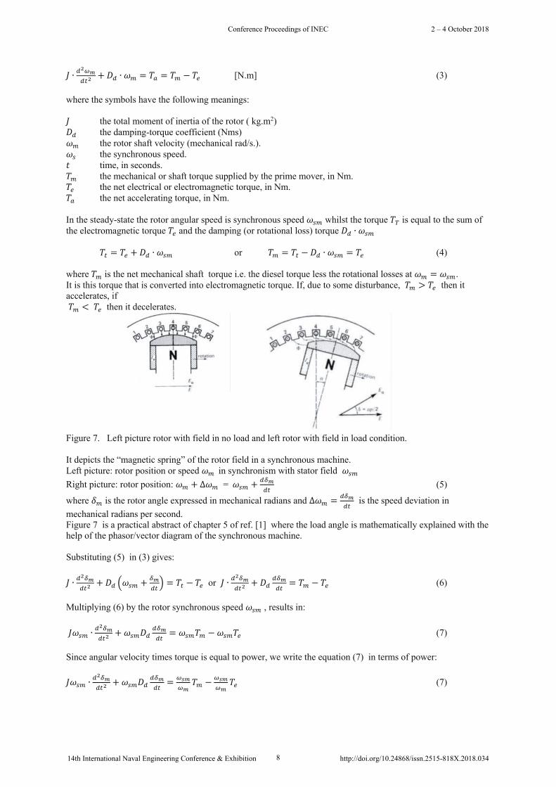
Figure 7. Left picture rotor with field in no load and left rotor with field in load condition.

It depicts the “magnetic spring” of the rotor field in a synchronous machine. Left picture: rotor position or speed 𝜔' in synchronism with stator field 𝜔L' Right picture: rotor position: 𝜔' + ∆𝜔' =𝜔L' +

ERGEH

(5)

where 𝛿' is the rotor angle expressed in mechanical radians and ∆𝜔' = ERGEH

is the speed deviation in mechanical radians per second. Figure 7 is a practical abstract of chapter 5 of ref. [1] where the load angle is mathematically explained with the help of the phasor/vector diagram of the synchronous machine.

Substituting (5) in (3) gives:

𝐽 ∙ E1RGEH1

+ 𝐷E T𝜔L' +RGEHU = 𝑇H − 𝑇K or 𝐽 ∙ E

1RGEH1

+ 𝐷EERGEH

= 𝑇' − 𝑇K (6)

Multiplying (6) by the rotor synchronous speed 𝜔L' , results in:

𝐽𝜔L' ∙E1RGEH1

+ 𝜔L'𝐷EERGEH

= 𝜔L'𝑇' − 𝜔L'𝑇K (7)

Since angular velocity times torque is equal to power, we write the equation (7) in terms of power:


+ 𝜔L'𝐷EERGEH

= FVGFG

𝑇' −FVGFG

𝑇K (7)



Where 𝑃' is the net shaft power input to the generator and 𝑃K is the electrical air-gap power, both expressed in watts. During a disturbance the speed of a synchronous machine is normally quite close to synchronous speed so that 𝜔' ≈ 𝜔L' and equation (7) becomes:


+ 𝜔L'𝐷EERGEH

= 𝑃' − 𝑃K (8)

The quantity 𝐽𝜔L' is called the inertia constant and is denoted by 𝑀' allows equation (8) to be written as:

𝑀' ∙E1RGEH1

= 𝑃' − 𝑃K − 𝐷'ERGEH

(9)

Where 𝐷' = 𝜔L'𝐷E is the damping coefficient. Equation (9) is called the swing equation.

It is common practice to express the angular momentum of the rotor in terms of a normalized inertia constant when all generators of a particular type will have similar inertia values regardless of their rating. The inertia constant is given the symbol 𝐻defined as the stored kinetic energy in megajoules at synchronous speed divided by the machine rating 𝑆\ in MVA so that

𝐻 = +.]^FVG1

_` and 𝑀' =

"a_`FVG

(10)

The units of 𝐻 are seconds. In effect 𝐻 simply quantifies the kinetic energy of the rotor at synchronous speed in terms of the number of seconds it would take the generator to provide an equivalent amount of electrical energy when operating at a power output equal to its MVA rating. Also used is the symbol 𝑇' as the mechanical time constant where:

𝑇' =^FVG1

_`= 2𝐻 and 𝑀' =

NG_`FVG

(11)

Again the units are seconds but the physical interpretation is different. In this case, if the generator is at rest and a mechanical torque equal to _`

FVG is suddenly applied to the turbine shaft, the rotor will accelerate, its velocity

will increase linearly and it will take 𝑇' seconds to reach synchronous speed 𝜔L' . The load angle is normally expressed in electrical radians and there mechanical equivalent is;

𝛿' = Rcd/"

and 𝜔L' = FVd/"

(12)

Where 𝑝 is the number of poles. Substituting equation (12) into equation (9) allows the swing equation to be written as:

"a_`FV

∙ E1REH1

+ 𝐷 EREH= 𝑃' −𝑃K or NG_`

FV∙ E

1REH1

+ 𝐷 EREH= 𝑃' −𝑃K (13)

When we neglect the losses : "a_`FV

∙ E1REH1

= 𝑃' −𝑃K (14) We can also write:

a_`g∙h

∙ E1REH1

= 𝑃' −𝑃K or 𝑀 ∙ E1REH1

= 𝑃' − 𝑃K (15)

This equation , is called the swing equation and it describes the rotor dynamics for a synchronous machine (generating/motoring). It is a second order differential equation where the damping term (proportional to 𝑑𝛿/𝑑𝑡 is absent because of the assumption of a lossless machine ). The electrical power equation in terms of 𝑃KGjk is: 𝑃K = 𝑃' − 𝑃KGjk ∙ 𝑠𝑖𝑛𝛿K (16) See for an extensive description reference [1] , [3] and [7]. Since, the mechanical power input 𝑃' and the maximum power output of the generator 𝑃KGjk are known for a given system topology and load, we can find the rotor angle 𝛿 from (16) as:



𝛿K = 𝑠𝑖𝑛o$ p qGqcGjk

r or 𝜋 − 𝑠𝑖𝑛o$ p qGqcGjk

r

It can be observed from (15) that the rotor angle 𝛿K has two solutions at which 𝑃' = 𝑃KGjk ∙ 𝑠𝑖𝑛𝛿K Now, let us label

𝛿Kt = 𝑠𝑖𝑛o$ p qGqcGjk

r and 𝛿KGjk = 𝜋 − 𝑠𝑖𝑛o$ p qGqcGjk

r

There is a very important implication of the two solutions u𝛿Kt, 𝛿KGjkv of equation (15) on the stability of the system. This can be clearly understood from what is called as “swing curve” or 𝑃 − 𝛿Kt curve.

Figure 8. Swing curve or 𝑃 − 𝛿Kt .

The swing curve is depicted in Figure 8. The swing curve shows the plot of electrical power output of the generator 𝑃K with respect to the rotor angle 𝛿K. As can be observed from Figure 8 the curve is a sine curve with 𝛿K varying from 0𝑡𝑜𝜋. The maximum power output of the generator 𝑃KGjk occurs at an angle 𝛿K = 𝜋/2. On the same curve the input mechanical power 𝑃' can also be represented. Since 𝑃' is assumed the be constant and does not vary with respect to 𝛿K , a straight line is drawn which cuts the 𝑃 − 𝛿Kt curve at points A and D. It can be seen from Figure 10 that at points A and D the mechanical power input 𝑃' is equal to 𝑃K. The rotor angles at point A and D are 𝛿Kt and 𝛿KGjk , the solutions of equation (15). Let us try to understand which of the solutions u𝛿Kt, 𝛿KGjkv leads to a stable operation. Let us take first point A. If we perturb the rotor angle 𝛿+ by a small positive angle ∆𝛿+, so that the new operating point is at B, then electrical power will also increase to 𝑃KGjk ∙ sin(𝛿+ + ∆𝛿+). So after perturbation 𝑃' <𝑃KGjk ∙ sin(𝛿+ + ∆𝛿+) , for a positive value of 𝛿+ . Now the output electrical power will be more than the input mechanical power and hence the rotor starts decelerating due to which the angle 𝛿 will be pulled back to the point A. But since the rotor has certain inertia it cannot stop at the point A and decelerate further due to which the angle 𝛿 moves to the point say C. At point C 𝑃' >𝑃KGjk ∙ sin(𝛿+ + ∆𝛿+) that is input mechanical power will be more than the electrical power output and hence the rotor starts accelerating. Again the rotor angle 𝛿 starts increasing and will reach point A but due to inertia it will again move to point B. This phenomenon repeats itself indefinitely if there is no damping to the rotor oscillations. This can be analogously understood from the pendulum motion in vacuum. If a pendulum is perturbed from its steady state position then it swings to one extreme point reverses it direction pass through its steady state position goes to the other extreme and reverse and pass through the extreme and this happens indefinitely as it is oscillating in vacuum and there is no air friction to stop the oscillations. Now take the case of second operating point 𝛿'J{. Again if we perturb 𝛿'J{ by a positive angle ∆𝛿'J{ then the electrical power output will be 𝑃KGjk sin(𝛿+ + ∆𝛿+)and the rotor starts accelerating due to which the angle will increased further and this will lead to further decrease in electrical output. Hence, for a small positive perturbation in the rotor angle at the operating point D leads to continuous increase in the speed of the rotor there by leading to unstable operation of the generator.

d

A

B

C

D

E



This discussion leads to an important conclusion that out of the two operating point B is unstable for small disturbances. Hence, point A is called stable equilibrium point and operating point D is called unstable equilibrium point. Similarly, 𝛿+ is a stable steady state rotor angle and 𝛿'J{ is an unstable rotor angle. From 𝑃 − 𝛿 curve it can be observed that if we disturb the rotor angle from point A by a small angle ∆𝛿 then the rotor angle starts oscillating between points B and C. If observed closely it can be seen that 𝑃 − 𝛿 curve falling between the points B and C is almost linear if ∆𝛿 is very small. Hence, if the rotor angle perturbation ∆𝛿 is very small then we can assume that the system behaves in a linear fashion around the operating point A between B and C. Mathematically this can be written by supposing the angle 𝛿+ is perturbed by an angle ∆𝛿 then we can express the swing equation as:

M∙ E1(Rt0∆R)EH1

= 𝑃' −𝑃KGjk ∙ sin(𝛿+ + ∆𝛿) (17)

using the formulae: sin(α+β) = sinα.cosβ + cosα.sinβ we get:

𝑀 ∙ E1RtEH1

+ 𝑀 ∙ E1∆REH1

= 𝑃' −𝑃KGjk ∙ (sin 𝛿+ ∙ 𝑐𝑜𝑠∆𝛿 + 𝑐𝑜𝑠𝛿+ ∙ 𝑠𝑖𝑛∆𝛿) (18)

since ∆𝛿 is small, 𝑐𝑜𝑠∆𝛿 ≅ 0 and 𝑠𝑖𝑛∆𝛿 ≅ ∆𝛿 with ∆𝛿 = 𝑟𝑎𝑑, we have:

𝑀 ∙ E1RtEH1

+ 𝑀 ∙ E1∆REH1

= 𝑃' −𝑃KGjk ∙ sin(𝛿+) −𝑃KGjk ∙ cos(𝛿+ ∙ ∆𝛿) (19)

Since at the initial operating point A,

𝑀 ∙ E1REH1

= 𝑃' − 𝑃KGjk ∙ 𝑠𝑖𝑛𝛿 = 0

𝑀 ∙ E1REH1

= −𝑃KGjk ∙ cos 𝛿 ∙ ∆𝛿 (20)

We can label, 𝑃L = 𝑃KGjk ∙ 𝑐𝑜𝑠𝛿+ 𝑃L is called as the synchronizing torque or power, as per units torque and power will be the same. 𝑃L is the torque required to pull the rotor in to synchronization. Substituting 𝑃L in (20) and rewriting it we can get:

𝑀 ∙ E1REH1

+ 𝑃L ∙ cos 𝛿+ = 0 (21)

The solution of the above second order differential equation depends on the roots of the characteristic equation given by

𝑠" = −𝑀 ∙ 𝑃L (22)

When 𝑃L is negative, we have one root in the right-half s-plane, and the response is exponentially increasing and stability is lost. When 𝑃L is positive, we have two roots on the 𝑗 − 𝜔 axis, and the motion is oscillatory and undamped. The system is marginally stable with a natural frequency of oscillation given by:

𝜔\ = 4𝑀 ∙ 𝑃L (23)

In case of a synchronous generator, the rotor has damper windings due to which it acts as an induction motor during transients and this effect has to be considered while evaluating the stability of the system. This effect of damper winding is called as damping torque which depends on the rate of change of rotor angle.

𝑃E = 𝐷 EREH

(24)

Where, 𝐷 is the damping coefficient. After including damping torque, the swing equation (15) can be written as:

𝑀 ∙ E1REH1

+ 𝐷 ∙ EREH+ 𝑃L∆𝛿 = 0 (25)



4 Introduction to the modelling

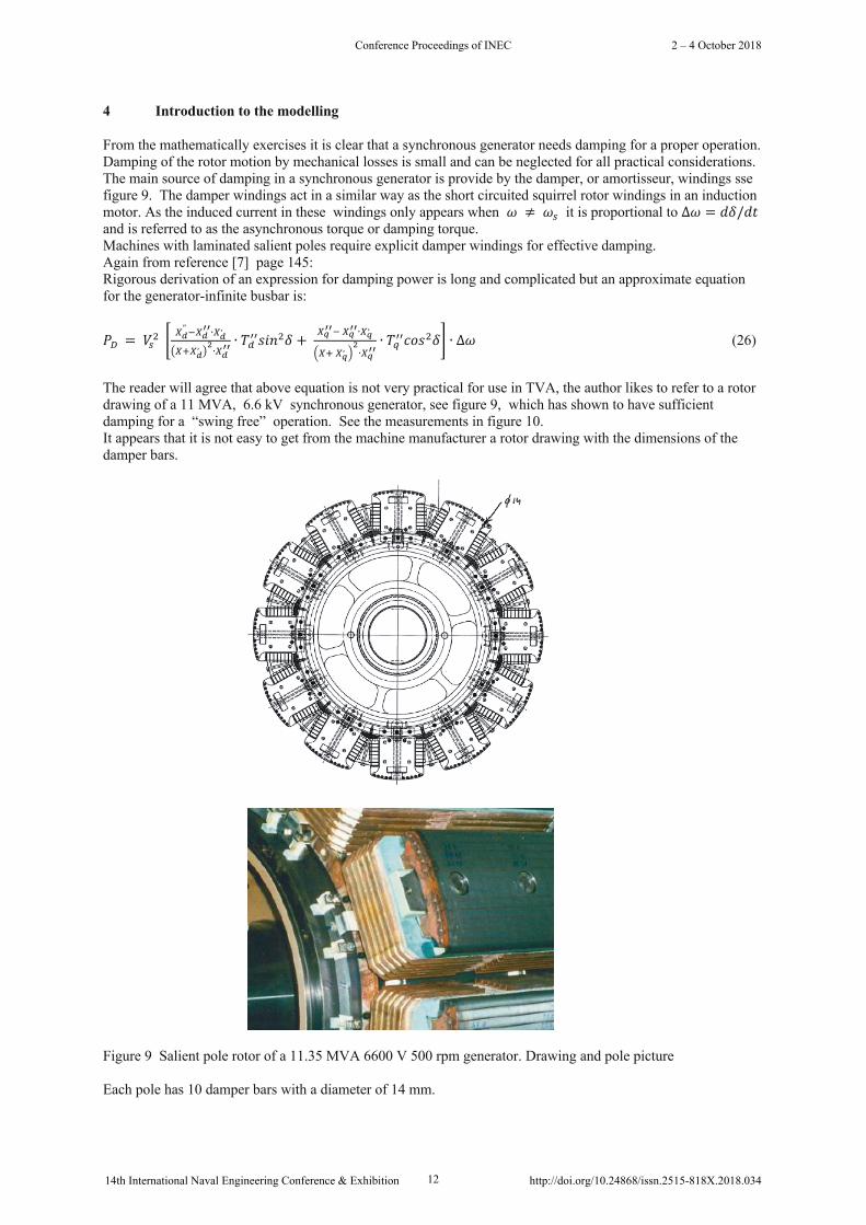
From the mathematically exercises it is clear that a synchronous generator needs damping for a proper operation. Damping of the rotor motion by mechanical losses is small and can be neglected for all practical considerations. The main source of damping in a synchronous generator is provide by the damper, or amortisseur, windings sse figure 9. The damper windings act in a similar way as the short circuited squirrel rotor windings in an induction motor. As the induced current in these windings only appears when 𝜔 ≠ 𝜔L it is proportional to ∆𝜔 = 𝑑𝛿/𝑑𝑡 and is referred to as the asynchronous torque or damping torque. Machines with laminated salient poles require explicit damper windings for effective damping. Again from reference [7] page 145: Rigorous derivation of an expression for damping power is long and complicated but an approximate equation for the generator-infinite busbar is:

𝑃� = 𝑉L" ��" o��

��∙��,

u�0��, v1∙�� ∙ 𝑇E

��𝑠𝑖𝑛"𝛿 +��o��∙��

,

T�0��, U1∙��

∙ 𝑇��𝑐𝑜𝑠"𝛿� ∙ ∆𝜔 (26)

The reader will agree that above equation is not very practical for use in TVA, the author likes to refer to a rotor drawing of a 11 MVA, 6.6 kV synchronous generator, see figure 9, which has shown to have sufficient damping for a “swing free” operation. See the measurements in figure 10. It appears that it is not easy to get from the machine manufacturer a rotor drawing with the dimensions of the damper bars.

Figure 9 Salient pole rotor of a 11.35 MVA 6600 V 500 rpm generator. Drawing and pole picture

Each pole has 10 damper bars with a diameter of 14 mm.



Also the mentioned exercises will not give a model for use in torsional vibration analysis. As mentioned in the introduction a practical approach is to regard the synchronous generator as a torsional spring, the rotor inertia is coupled magnetically to the grid inertia and through the grid inertia magnetically coupled to another generator in case of parallel service. So a ship’s power plant with generator sets running parallel appears to be a complicated dynamic system and needs proper design and engineering to ensure stable parallel operation of the generator set’s. The magnetic stiffness can be derived from the load angle data at different loads, see the calculations at page 15.

4.1 Measurements showing a swing free parallel operation

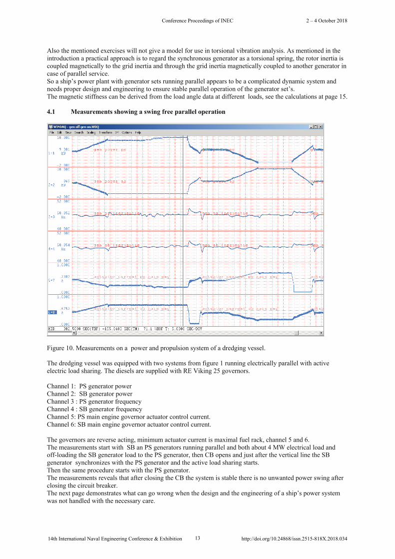
Figure 10. Measurements on a power and propulsion system of a dredging vessel.

The dredging vessel was equipped with two systems from figure 1 running electrically parallel with active electric load sharing. The diesels are supplied with RE Viking 25 governors.

Channel 1: PS generator power Channel 2: SB generator power Channel 3 : PS generator frequency Channel 4 : SB generator frequency Channel 5: PS main engine governor actuator control current. Channel 6: SB main engine governor actuator control current.

The governors are reverse acting, minimum actuator current is maximal fuel rack, channel 5 and 6. The measurements start with SB an PS generators running parallel and both about 4 MW electrical load and off-loading the SB generator load to the PS generator, then CB opens and just after the vertical line the SB generator synchronizes with the PS generator and the active load sharing starts. Then the same procedure starts with the PS generator. The measurements reveals that after closing the CB the system is stable there is no unwanted power swing after closing the circuit breaker. The next page demonstrates what can go wrong when the design and the engineering of a ship’s power system was not handled with the necessary care.



4.2 Undocumented measurements of a dynamic system with among other things insufficient damping

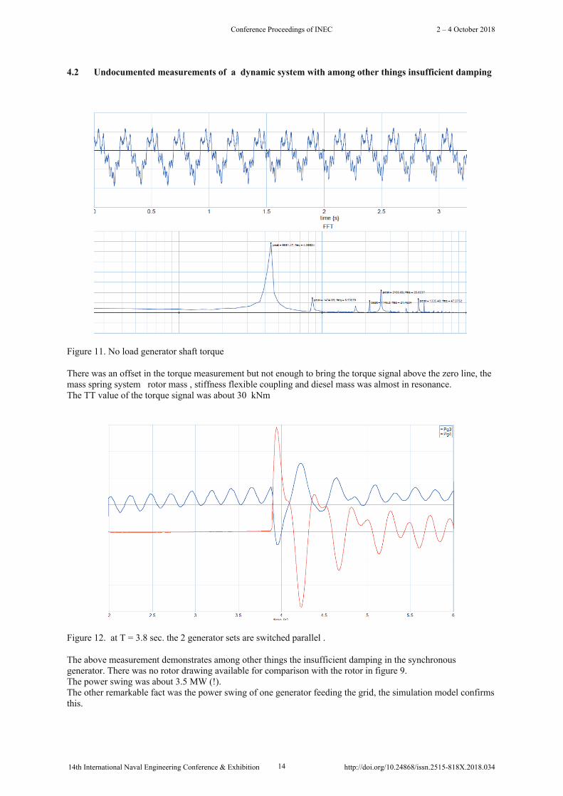
Figure 11. No load generator shaft torque

There was an offset in the torque measurement but not enough to bring the torque signal above the zero line, the mass spring system rotor mass , stiffness flexible coupling and diesel mass was almost in resonance. The TT value of the torque signal was about 30 kNm

Figure 12. at T = 3.8 sec. the 2 generator sets are switched parallel .

The above measurement demonstrates among other things the insufficient damping in the synchronous generator. There was no rotor drawing available for comparison with the rotor in figure 9. The power swing was about 3.5 MW (!). The other remarkable fact was the power swing of one generator feeding the grid, the simulation model confirms this.



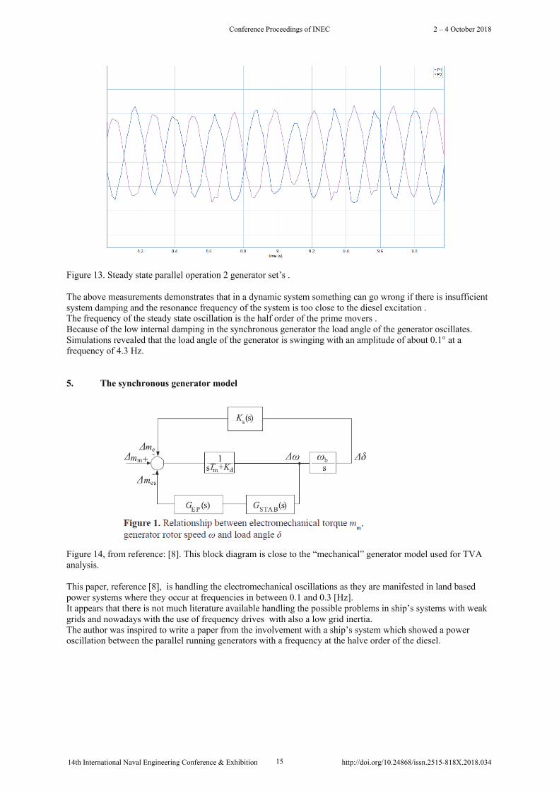
Figure 13. Steady state parallel operation 2 generator set’s .

The above measurements demonstrates that in a dynamic system something can go wrong if there is insufficient system damping and the resonance frequency of the system is too close to the diesel excitation . The frequency of the steady state oscillation is the half order of the prime movers . Because of the low internal damping in the synchronous generator the load angle of the generator oscillates. Simulations revealed that the load angle of the generator is swinging with an amplitude of about 0.1° at a frequency of 4.3 Hz.

5. The synchronous generator model

Figure 14, from reference: [8]. This block diagram is close to the “mechanical” generator model used for TVA analysis.

This paper, reference [8], is handling the electromechanical oscillations as they are manifested in land based power systems where they occur at frequencies in between 0.1 and 0.3 [Hz]. It appears that there is not much literature available handling the possible problems in ship’s systems with weak grids and nowadays with the use of frequency drives with also a low grid inertia. The author was inspired to write a paper from the involvement with a ship’s system which showed a power oscillation between the parallel running generators with a frequency at the halve order of the diesel.



5.1 Model parameters of the synchronous generator

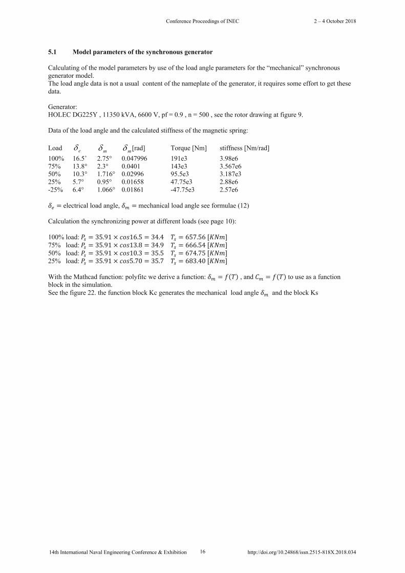
Calculating of the model parameters by use of the load angle parameters for the “mechanical” synchronous generator model. The load angle data is not a usual content of the nameplate of the generator, it requires some effort to get these data.

Generator: HOLEC DG225Y , 11350 kVA, 6600 V, pf = 0.9 , n = 500 , see the rotor drawing at figure 9.

Data of the load angle and the calculated stiffness of the magnetic spring:

Load [rad] Torque [Nm] stiffness [Nm/rad] 100% 16.5˚ 2.75° 0.047996 191e3 3.98e6 75% 13.8° 2.3° 0.0401 143e3 3.567e6 50% 10.3° 1.716° 0.02996 95.5e3 3.187e3 25% 5.7° 0.95° 0.01658 47.75e3 2.88e6 -25% 6.4° 1.066° 0.01861 -47.75e3 2.57e6

𝛿K = electrical load angle, 𝛿' = mechanical load angle see formulae (12)

Calculation the synchronizing power at different loads (see page 10):

100% load:𝑃L = 35.91 × 𝑐𝑜𝑠16.5 = 34.4 𝑇L = 657.56[𝐾𝑁𝑚] 75% load:𝑃L = 35.91 × 𝑐𝑜𝑠13.8 = 34.9 𝑇L = 666.54[𝐾𝑁𝑚] 50% load:𝑃L = 35.91 × 𝑐𝑜𝑠10.3 = 35.5 𝑇L = 674.75[𝐾𝑁𝑚] 25% load:𝑃L = 35.91 × 𝑐𝑜𝑠5.70 = 35.7 𝑇L = 683.40[𝐾𝑁𝑚]

With the Mathcad function: polyfitc we derive a function: 𝛿' = 𝑓(𝑇) , and 𝐶' = 𝑓(𝑇) to use as a function block in the simulation. See the figure 22. the function block Kc generates the mechanical load angle 𝛿' and the block Ks

ed md md



6. The model for torsional vibration analysis.

The purpose of this modelling is to investigate the torsional vibration behaviour of the system , a diesel engine with on the flywheel side a flexible coupling with a clutch then a reduction gearbox, propeller shaft with the propeller, and on the PTO side a flexible coupling with a generator. See figure 15.

Figure 15. Complete torsional vibration analysis model.

The iconic model is self explaining and on the next pages the bond graph within the icons will be clearyfied.

It appears that a thermodynamic model of the combustion to generate the combustion force on the piston is interesting but too complicated for this purpose. A practical approach to model the combustion pulse was found in reference [4], page 198 . For the piston force a cosine shaped variable is chosen, to be max. in the upper dead point and min. in the lower dead point. Another advantage is that for dynamic analysis of the speed control of the diesel the fuel pump delay is automatic taken into account. Figure 16. depicts how to generate this combustion signal with the help of some iconic models from the 20Sim library. Torque measurements reveals that this approach generates a simulation output close to the measurements. As the inertia of the generator in much more than the diesel inertia the rotational speed is more even , thanks to the Vulkan coupling, the governor speed sensing is performed from the shaft of the generator rotor, the back-up speed sensing is from the diesel flywheel.

12V46diesel

camshaft drive

Vulkan +Meslu clutch

Clutch_in

Clutch_out

Diesel_12V46

1

5

3

6

2

4

Firing order

Fuelinjection

Gearbox

Gen_1

Gov 1

Grid

KW_G1

Misfiring

Propeller_1

S_point speed

Vulkan_1



6.1 Combustion pulse generator

Figure 16 . Iconic model to generate the combustion pulse.

The diesel engine involved is a Wärtsilä 12V46 engine, the V angle is 45° degrees = 0.7853 rad..

Figure 17 Simulation output of the model of figure 15.

The black line is the combustion pulse, max. at upper dead point an min. at lower dead point. Comparing the FFT of the output torque of the diesel measurements and the FFT of the simulation of the diesel output torque this matches realistically.

Figure 18. The combined combustion pulse for a V engine.

To speed up the simulation process the iconic blocks are replaced by 20Sim code to generate the combustion pulses, see appendix 1.

- 0.7853 [rad]

+ 1

+ 1

And

And1

K

Comb_pulse

Constant

Constant1

Constant2

Constant3

cos

Cosine

cos

Cosine1

∫Integrate K

Pule_A

K

Pule_B

sin

Sine

sin

Sine1

Plot

0 2 4 6 8 10rad

-2

-1

0

1

2

3sinus1 + cosinePulse_A

Plot

0 2 4 6 8 10rad

0

1

2

3

4Pulse_A + Pulse_B



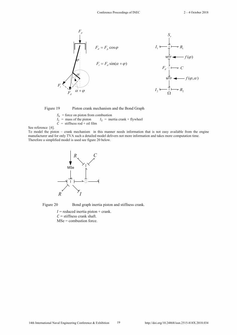
Figure 19 Piston crank mechanism and the Bond Graph 𝑆K = force on piston from combustion 𝐼$ = mass of the piston 𝐼" = inertia crank + flywheel 𝐶 = stiffness rod + oil film

See reference [4]. To model the piston – crank mechanism in this manner needs information that is not easy available from the engine manufacturer and for only TVA such a detailed model delivers not more information and takes more computation time. Therefore a simplified model is used see figure 20 below.

Figure 20 Bond graph inertia piston and stiffness crank.

𝐼 = reduced inertia piston + crank. 𝐶 = stiffness crank shaft. MSe = combustion force.

MTF

MTF

)(jf

),( ajf

dF

W 2R

1R

C

eS

j

a

ja +dF

tF

)sin( ja += dt FF

jcospd FF =

pF

1I

2I

MSe

R C

R I



6.2 Diesel rotating parts model

Figure 21. BG model elastic system 12V46 engine crank shaft.

On the right side the 6 combined cylinder inertia’s and on the left side the 6 torque pulses.

vulcan flange

camshaftdrive

shaft

A1/B1

A2/B2

A3/B3

A4/B4

A5/B5

A6/B6

Flywheel +coupling flange

diesel PTO shaft

rpm

p

input2

input3

input4

input5

input6

input7

CC10

CC11

CC4

CC5

CC6

CC7

CC8

CC9

II10

II11

II12

II4

II5

II6

II7

II8

II9

LPFFO

LowPassFilter1

MSeMSe1

MSeMSe4

MSeMSe5

MSeMSe6

MSeMSe8

MSeMSe9

1OneJunction10

1OneJunction11

1OneJunction12

1OneJunction13

1OneJunction14

1OneJunction15

1OneJunction16

1OneJunction17

1OneJunction18

1OneJunction19

1OneJunction20

1OneJunction21

1OneJunction22

1OneJunction23

1OneJunction7

1OneJunction8

1OneJunction9

RR10

RR11

RR12

RR13

RR14

RR15

RR16

RR17

RR18

RR19

RR20

RR21

RR22

RR23

RR7

RR8

RR9

0ZeroJunction10

0ZeroJunction11

0ZeroJunction4

0ZeroJunction5

0ZeroJunction6

0ZeroJunction7

0ZeroJunction8

0ZeroJunction9



6.3 Mechanical synchronous generator model

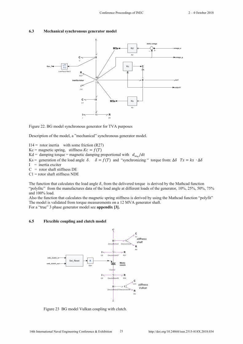
Figure 22. BG model synchronous generator for TVA purposes

Description of the model, a ”mechanical” synchronous generator model.

I14 = rotor inertia with some friction (R27) Kc = magnetic spring, stiffness 𝐾𝑐 = 𝑓(𝑇) Kd = damping torque = magnetic damping proportional with 𝑑F`/𝑑𝑡 Ks = generation of the load angle 𝛿. 𝛿 = 𝑓(𝑇) and “synchronizing “ torque from: ∆𝛿 𝑇𝑠 = 𝑘𝑠 ∙ ∆𝛿 I = inertia exciter C = rotor shaft stiffness DE C1 = rotor shaft stiffness NDE

The function that calculates the load angle 𝛿, from the delivered torque is derived by the Mathcad function “polyfitc” from the manufactures data of the load angle at different loads of the generator, 10%, 25%, 50%, 75% and 100% load. Also the function that calculates the magnetic spring stiffness is derived by using the Mathcad function “polyfit” The model is validated from torque measurements on a 12 MVA generator shaft. For a “true” 3 phase generator model see appendix [3].

6.5 Flexcible coupling and clutch model

Figure 23 BG model Vulkan coupling with clutch.

inertia rotor

delta omega

p

output1

p1

omega_e

omega_g

Gen_T

CC

CC1

CCm

II

II14

Kc

Kc

Kd

Kd

Ks

Ks

LPFFO

LowPassFilter3

MSe

MSe

1

1

RR1

RR27

0

0

0

stiffnessshaft

Mesluclutch

stiffness Vulkan

p

p1

cmb_clutch_in

cmb_clutch_out

CC2

CC23

Clutch2

Set_Reset K

Gain

II24

II25

1OneJunction4

1OneJunction49

1OneJunction50

1OneJunction51

RR3

RR4

RR50

RR51

0ZeroJunction2

0ZeroJunction23



The used clutch model is a simple clutch model from the 20Sim librarie and its suits for this purpose. Friction is not easy to model it in a proper way and again the auther refers to the literature available on this subject see [37]. And also the stiffness of the elastic element is modeled as a simple spring.

6.6 Gearbox model

Figure 24. BG model gearbox.

The model can be simplified by reducing the system to engine speed then the system simplifies to the gearbox inertia the propeller shaft stiffness and then the propeller inertia.

6.7 Propeller model

Figure 25. BG model of propeller shaft and propeller inertia and the 20Sim blocks to generator the first order propeller excitation.

inertia gearwheel

stiffnessshaft

inertia flange

gear ratio0.2347

gear mesh

inertia gearwheel

p

p1

CC16

CC4

II17

II2

II4

1OneJunction3

1OneJunction32

1OneJunction33

1OneJunction7

RR3

RR32

RR33

RR7

TFTF

0ZeroJunction16

0ZeroJunction4

stiffnessprop.shaft

inertiapropeller

first order propellerexcitation

p

CC1

K

Gain

K

Gain1

II1

Integrate

MSeMSe

1OneJunction1

1OneJunction2

RR1

RR2

sin

Sine

0ZeroJunction1



6.8 Simple speed governor model

Figure 26. Simplified model of the Viking 25 governor.

As depicted this is a simplified model, normally the governor has a some more variable gains as there are: error dependable gain( small error low gain big error high gain), speed dependable gain, error dependable integration time. See appendix 2 for a detailed block diagram. In the model there is only load dependable gain and load dependable integration time and error dependable derivation time (big error no derivation , small error some derivation) . The dynamics of a governor are determined by the actuator to move the lever of the fuel pumps see again appendix 2 for a block diagram of the hydraulic actuator, the up/down time of the actuator is about 80 msec. so the actuator is modelled as a fist order system with a time constant of 80 msec. The modern diesel is now a common rail engine and this engine is much better to control, today necessary to comply with the exhaust emission rules, the controller output is direct input to the fuel injector.

6.9 The flexible coupling

Another object of interest is the flexible coupling, in this simulation model, modelled as a simple spring with damping. As depicted in the icon in figure 15 there is a flexible coupling between the diesel and generator and a second one between the diesel and the propulsion gearbox.

The author was able to do some measurements during a commissioning at the Vulkan factory in Herne (years ago but the physics of the rubber elements do not change) and an abstract of the analysis of the measurements will be given see pages 25 and 26. For interesting literature regarding this subject see [30], [31], [32], [33], [34].

Unfortunately this literature does not present a “usable” rubber model for use in a TVA model. The analysis of the measurements revealed that a rubber coupling element is a highly nonlinear peace of material, at low oscillating torque amplitude there is no damping and at high oscillating torque there is considerable damping. Regarding the stiffness at low oscillating torque amplitude there is high dynamic stiffness and at high oscillating torque amplitude the dynamic stiffness is lower. This nasty habit of the rubber elements in a flexible coupling played an important role in the project with unpleasant oscillations ( see figure 11 , 12 and 13), unfortunately the flow of information is blocked by a NDA agreement. The flexible coupling (Vulkan_1) between the diesel and generator is a model with stiffness and damping adaption derived from the Vulkan measurements and the Vulkan data sheet during a commissioning at their factory. The Author developed a “usable” coupling model

sp speed

mv speed

output stage +hydraulic actuator

input

plus

output

kd 2 fh ss + 2 fh

Differentiate

LP-1Butterworth

Filter1Integrate1

K

Kd

K

Ki

K

Kp

LPFFO

LowPassFilter1

LPFFO

LowPassFilter2

K

NLGi

K

NLGp

NLG_I

NLG_P

NLG_P2

PlusMinus1 PlusMinus2Splitter2 Splitter5



Figure 27. BG model flexible coupling with adaption block. The adaption block has 2 outputs, output Kd is the elastic element damping adoption signal and output Kc is the elastic element stiffness adoption signal.

Figure 28. inside the adaption block.

The Tk_w block determines the amplitude of the oscillating torque superimposed upon the mean torque and the right blocks determines the adaption factor for the damping and the stiffness of the elastic element.

In the Vulkan performance data the Vibratory Torque TW is specified as: “The vibratory torque Tw is the amplitude of the fluctuating torque superimposed upon the mean torque Tm in the stationary condition, Tw should not exceed the permissible maximum vibratory torque Tkw ”. See reference [38].

The adaption block is not complete, the internal warming up of the element is not yet modelled . To use this elastic coupling model is also useful at starting the model, starting of the diesel generates high oscillating torque in the element and can cause numeric instability

6.10 The grid model.

Figure 29. Simple grid model. The grid is modelled as an inertia (I31) with a resistive load (R60) ,input1 is the increasing load command input and the grid inertia is also increased with the load. Please note that the grid inertia has to be transformed to the diesel speed and that means that the grid inertia has to be multiplied by a factor 36. The generator has 6 pole pairs ( 50 Hz) , so the factor is 62. When there are some big direct on-line electrical motors than the grid inertia can be considerable and has a low damping to the possible electrical power oscillations . Simulations depicts that a low grid inertia has more damping than a high grid inertia.

Vulcan flange

pp1

output1

AdaptionKd

Kc

Adaption

CC3

II16

1

1

RR29 R

R6

0

input

outputoutput1

output11

increase/decrease Kc

up_down Kd

Limit1

Tk_w

Tk_w

inertia + loadmains

p

omega_e

input1II31

1

RR60



7. Some measurements of a Vulkan flexible element.

Figure 30. Element 27RTR , x axis applied torque y axis angle of deflection Temperature element is 30°. Pre torque of 20 kNm. Amplitude oscillating torque: 4.3 kNm top-top. Dynamic stiffness is 1411 kNm/rad. Notice that the element has almost no damping.

Figure 31 Element 27RTR. , x axis applied torque y axis angle of deflection Temperature element is 30°. Pre torque of 20 kNm. Amplitude oscillating torque: 16.67 kNm top-top. Dynamic stiffness is 645.1 kNm/rad. Notice that the element has now damping, the width of the banana is a the amount of damping.



7.1 Mathcad plot of damping versus oscillating torque

Figure 32. Plot from the Vulkan measurements.

x axis: ∆𝑇[𝑘𝑁𝑚] y axis: damping amplification factor

7.3 Mathcad plot of stiffness versus oscillating torque

Figure 33. Plot from the Vulkan measurements.

Stiffness as a function of the amplitude of the oscillating torque x axis: ∆𝑇[𝑘𝑁𝑚] y axis: stiffness reducing factor

The above plots demonstrates the nonlinear properties of rubber elements of a flexible coupling. In a proper engineered system the resonance frequencies are more than a factor √2 from the system excitations than the system works fine with the stiffness parameters from the manufactures data sheet. Also an important property is that at increasing temperature of the elements the stiffness is decreasing. See also reverence [34].



8. Simulation results.

Figure 34. Simulation output.

Plot 1: diesel speed [rad/sec] Plot 2: generator shaft torque [Nm] Plot 3: propeller shaft torque [Nm] Plot 4: generator electrical power.[W]

At t = 0 the diesel starts and speed up to half nominal speed, at t = 10 seconds the propeller in clutched-in and at t = 15 seconds the diesel speeds up to nominal speed = 500 rpm = 52.4 [rad/sec]. At t = 25 seconds the electrical generator load is increased to 4e6 [W]. The simulation depicts that there are no resonances in the speed range of the diesel.

Figure 35. Simulation output no load toque in generator shaft.

The first peak in the FFT plot is the halve order of the diesel, the second smaller peak is the first order of the diesel.

20

40

60

80 Diesel speedrad/sec

050000

100000150000200000250000 Gen_T

Nm

0100000200000300000400000500000 Prop_shaft_T

Nm

0 5 10 15 20 25 30 35 40time {s}

0

1e+006

2e+006

3e+006

4e+006 E powerW

0 2 4 6 8 10X {s}

0

20000

40000

60000

80000

Gen_TNm

FFT

1 10 100Frequency [Hz]

-1000

0

1000

2000

3000

4000FFT:Nm

peak = 2835.19; freq = 4.20168

peak = 947.907; freq = 71.2285peak = 591.158; freq = 8.40336peak = 513.352; freq = 50.2201

peak = 403.27; freq = 67.0268



Figure 36. Simulation output no load torque propeller shaft. The model is generating the same torque signal as measured in the propeller shaft see figure 37.

Figure 37. no load torque measurement propeller shaft.

The shaft torque measurement had an output of 118.5 kNm/V, so the vertical scaling is 6.97 kNm/div. The horizontal scaling is 0.28 sec/div. Literature/manufacture’s documentation revealed that the entrained water of the propeller should be taken into account and in case of a controllable pitch propeller the entrained water depends on the pitch. That implies that the resonance frequency in the system is changing with the pitch of the propeller. The Author has never measured a changing resonance frequency due to the changing pitch of the propeller.

Propshaft T

0 2 4 6 8 10 12time {s}

0

20000

40000

60000

80000

100000

120000

140000

160000

180000[Nm]



9. Torsional vibration analysis complete power and propulsion plant.

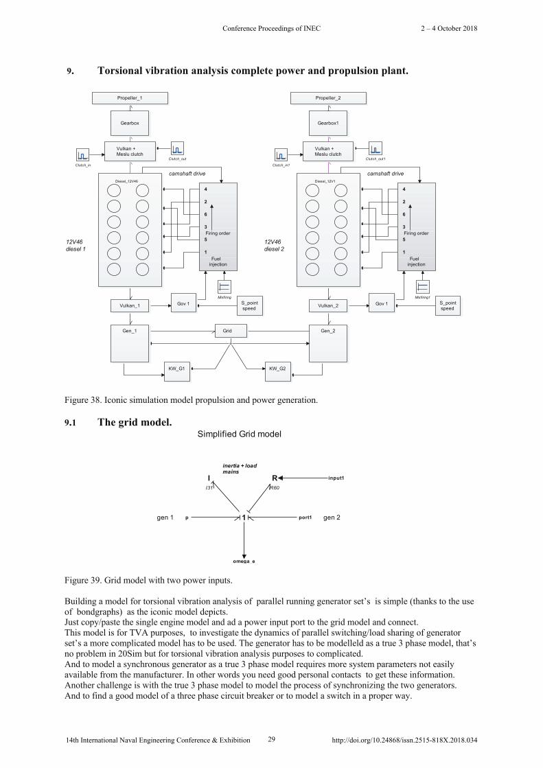
Figure 38. Iconic simulation model propulsion and power generation.

9.1 The grid model.

Figure 39. Grid model with two power inputs.

Building a model for torsional vibration analysis of parallel running generator set’s is simple (thanks to the use of bondgraphs) as the iconic model depicts. Just copy/paste the single engine model and ad a power input port to the grid model and connect. This model is for TVA purposes, to investigate the dynamics of parallel switching/load sharing of generator set’s a more complicated model has to be used. The generator has to be modelleld as a true 3 phase model, that’s no problem in 20Sim but for torsional vibration analysis purposes to complicated. And to model a synchronous generator as a true 3 phase model requires more system parameters not easily available from the manufacturer. In other words you need good personal contacts to get these information. Another challenge is with the true 3 phase model to model the process of synchronizing the two generators. And to find a good model of a three phase circuit breaker or to model a switch in a proper way.

12V46diesel 1

camshaft drive

12V46diesel 2

camshaft drive



Clutch_in Clutch_in1

Clutch_out Clutch_out1

Diesel_12V1Diesel_12V46

1

5

3

6

2

4

Firing order

Fuelinjection

1

5

3

6

2

4

Firing order

Fuelinjection

Gearbox Gearbox1

Gen_1 Gen_2

Gov 1 Gov 1

Grid

KW_G1 KW_G2

Misfiring Misfiring1

Propeller_1 Propeller_2

S_point speed

S_point speedVulkan_1 Vulkan_2

inertia + loadmains

gen 1 gen 2

Simplified Grid model

p

input1

omega_e

port1

II31

1

RR60



To get a good block diagram of the working of a synchronizer is not easy.

Figure 40. Simulation output .

Above plots are speed of diesel 1 with the generator 1 shaft torque. The below plots are speed of diesel 2 with the generator 2 shaft torque

As the interest are the torsional vibrations the diesels starts simultaneously and speed up to nominal speed. To investigate the dynamics of parallel switching of the generators than this model is to simple. Then there is the need for a “true” 3 phase synchronous generator model see appendix 3 .

diesel 1

0 5 10 15 20 25 30 35 40time {s}

0

10

20

30

40

50

60

70

80

90

100rpm

diesel 2

0 5 10 15 20 25 30 35 40time {s}

0

10

20

30

40

50

60

70

80

90

100rpm

gen 1

0 5 10 15 20 25 30 35 40time {s}

0

50000

100000

150000

200000Gen1_T

gen 2

0 5 10 15 20 25 30 35 40time {s}

0

50000

100000

150000

200000Gen2_T



Conclusions.

The synchronous 3 phase generator appears to be a highly dynamic system. It is not easy to get “usable” data regarding the damping torque of a synchronous generator, see for an explanation [39]. This paper depicts the power of Bond Graphs in modeling marine engineering systems. The first problem for a control engineer or systems engineer in front of a process to control is to obtain a precise and easily manipulated model with predictions corresponding to the real observations. The use of 20sim as a simulation package make live a lot easier because of the ability of direct input of the Bond Graph. For people not familiar with Bond Graphs there is a large library of iconic models see www.20Sim.com. The modeling itself is broaden the insight and understanding of the system. The most time consuming part of modeling is to get the right parameters of the system or the systems components. It depends largely on knowing the right man on the right place to get the information needed to set up a model that represent the physical system. Measurements revealed that the simplifications, among other things the generation of the combustion pulses, in the modeling where allowed for this reason finding the resonance frequencies of the system, as mentioned before one looks for relevant analogies, not for complex identities. Unfortunately the system involved and the mentioned measurements were not allowed to use in this paper.



REFERENCES

[1] Modeling for transient torsional vibration analysis in marine power train systems.Kristine Bruun, Eilif Pedersen and Harald Valland.The Norwegian University of Science and TechnologyDepartment of Marine Technology.

[2] J.P. den Hartog. Mechanical Vibrations Dover, 1985.ISBN 0-486-64785-4

[3] Power Systems Analysis, Hadi Saadat[4] S.T. Nannenberg. Bondgraaftechniek (in Dutch) Delta Press,

1987 ISBN 90-6674-1256[5] Dean C. Karnopp, Donand L. Marlolis, Ronald C. Rosenberg. System Dynamics John Wiley. 2000

ISBN 0-471-33301-8[6] Jean U. Thoma. Simulation by Bondgraphs. Intoroduction to a Graphical Method

Springer, 1990 ISBN 3-540-51640-9 (very good for the practical engineer)[7] Power System Dynamics and Stability

Jan Machowski, Janus W.Bialek, James R. Bumby. John Wiley & Sons.[8] Stabilization of the Electrotromechanical Oscillations of Synchronous Generator

Damir Sumina1) , Neven Bulic1) and Srdan Skok2)

1)Faculty of Electrical Engineering and Computing. University of Zagreb2)Faculty of Engineering University of Ryeka

[9] Hallvard Engja. Modelling for transient performance simulation of diesel engines using Bond Graphs.ISME 1983, page 321 - 328.

[10] Hallvard Engja. The Bond graph technique as a powerful modeling tool. International symposium onAdvances in Marine Technology, page 471 - 441.

[11] Vulkan Technical data sheet: RATO-ETD[12] Hallvard Engja, Application of Bond graphs for mathematical modelling and simulation of marine

PTMC 2004 papers , pages 11 – engineering systems.Trans IMarEST, Vol 110, part 4 pp 229-239.

[13] P.J.Gawthrop, Bondgraphs: A representation for mechatronic systems. Mechatronics Vol 1, No. 2 pp127-156, 1991

[14] Peter Gawthrop,Lorcan Smith: Metamodelling: Bond graphs and dynamic systems. Prentice Hall ISBN0-13-489824-9

[15] P.C. Breedveld and G.Dauphin-Tanguy: Bond Graphs for Engineers. North-Holland 1992.[16] T.Heeringa: Engineering around a hydraulic controlled gearbox.

PTMC 2004 papers , pages 11 – 36.[17] J.Thoma B.Ould Bouamama: Modelling and Simulation in Thermal and Chemical Engineering.

Springer. ISBN 3-540-66388-6[18] D.A. Haessig, B. Friedland. On the Modeling and Simulation of Friction. Transactions of the ASME

Vol. 113, September 1991 pages 354 – 362.[19] T.Heeringa: Modelling and control of marine engineering systems.

PTMC 2006 papers, pages: 225 – 249.[20] Stationäres Betriebsverhalten der Synchronmachine am starren Netz, Prof. Dr.-Ing. Habil. U. Beckert.

TU Bergakademie Freiberg, Institut für Elektrotechniek[21] Electric Power Systems, B.M.Weedy, John Wiley & Sons.[22] Electrische Maschinen, Rolf Fischer, Carl Hanser Verlag[23] Elements of Power System Analysis, William D. Stevenson, Jr. McGraw-Hill.[24] Bond Graph Modeling of Marine Power Systems. Tom Arne Pedersen, Doctoral thesis at NTNU, 2009[25] Alternating Current Machines M. G. Say ELBS/Longman ( The AC machines book for the practical

engineer ).[26] Friction Models and Friction Compensation. H. Olsson1), K.J.Åström1) , M.Gäfvert1), C.Canudas de

Wit2), P.Lischinsky3).1) Department of Automatic Control, Lund Institute of Technology, Lund University, Lund.2) Laboratoire d’Automatique de Grenoble3) Control Department, EIS, ULA, Mérida 5101, VenezuelaThis paper has an extensive reference list.

[27] Kundur, P., Power System Stability and Control McGraw-Hill, 1993[28] Bond Graph Modelling of Engineering Systems. Wolfgang Borutzky Springer .[29] On dynamic properties of rubber isolators.

Doctoral Thesis Mattias Sjöberg, ISRN KTH/KT/D--02/39--SE[30] The elasticity and related properties of rubbers, (http://iopscience.iop.org/0034-4885/36/7/001)



[31] Engineering Viscoelasticity. David Roylance, Department of Materials Science and Engineering. MITCambridge, October 24, 2001.

[32] On the modelling of nonlinear elastomeric vibration isolators, Journal of Sound and Vibration (1999)219(2), 239-253.

[33] Influence of temperature on characteristics properties of flexible coupling. Jaroslav HOMISIN, PeterKASSAY, Department of Mechanisms. Faculty of Engineering, Technical University Kosice.

[34] Vulkan Couplings, Explanation of technical data. 08/2016.[35] https://tel.archives-ouvertes.fr/tel-00563111/document document in French[37] An alternative model for static and dynamic friction in dynamic system simulation. Peter J Breedveld.

1st IFAC-conference on Mechatronic systems, September 18-20, 2000 Darmstad, Germany, Vol 2, pp.717-722.

[38] Vulkan paper : VULKAN Couplings, Explanation of technical data for marine applications andstationary energy production. 08/2016. See: www.vulkan.com

[39] EP-Based Optimisation for Estimation Synchronising and Damping Torque CoefficientsN.A.M. Kamari, I. Musirin, Z.A. Hamid, M.N.A. RahimEnergy and Power 20123, 2(2): 17-23

[40] Introduction to Physical Systems Modelling with Bond Graphs, Jan F. Broenink.University of Twente.[41] A Bond Graph Approach for the Modelling and Simulation of a Buck Converter. Rached Zrafi, Sami

Ghedira and Kamel Besbes, University of Monastir, Monastir 5000, Tunesia. Journal of Low PowerElectronics and Applications.

[42] Modeling & Simulation 2018 . Lecture 8. Bond graphs Claudio Altafini Automatic Control, ISYLinköping University, Sweden



Appendix 1

20Sim code of the combustion pulse generator for a V12 engine

variables real a,c,d,f,g,i,j,l,m,o,p,x,z; real aa,cc,dd,ff,gg,ii,jj,ll,mm,oo,pp,xx,zz; real ww; boolean b, bb, e, ee, h, hh, k, kk, n, nn, q, qq; real port1, port2, port3, port4, port5, port6, port8, port9, port10, port11, port12, port13;

equations z = misfiring; zz = fuel; ww = speed * 0.5; x = sin ( ww * time); a = 1 + cos ( ww * time); b = if x > 0.01 and a > 0.01 then

true else

false end;

if b then port1 = zz *(0.99 * a); // pulse 1A

else port1 = 0;

end; xx = sin ( ww * time - 0.43633); // Vee angle 45 degrees. aa = 1 + cos ( ww * time - 0.43633); bb = if xx > 0.01 and aa > 0.01 then

true else

false end;

if bb then port8 = zz * aa; // pulse 1B

else port8 = 0;

end; cylin_1 = port1 + port8; c = sin ( ww * time - 1.0473); d = 1 + cos ( ww * time - 1.0473); e = if c > 0.01 and d > 0.01 then

true else

false end;

if e then port2 = zz*( 0.98 * d); // pulse 2A

else port2 = 0;

end; cc = sin ( ww * time - 1.4835); dd = 1 + cos ( ww * time - 1.4835); ee = if cc > 0.01 and dd > 0.01 then

true else

false end;

if ee then port9 = zz * (1.03 * dd); // pulse 2B

else port9 = 0;

end; cylin_2 = port2 + port9;



f = z * sin ( ww * time - 2.0944); g = z * ( 1 + cos ( ww * time - 2.0944)); h = if f > 0.01 and g > 0.01 then

true else

false end;

if h then port3 = zz * (0.97 * g); // pulse 3A

else port3 = 0;

end; ff = sin ( ww * time - 2.503); gg = 1 + cos ( ww * time - 2.507); hh = if ff > 0.01 and gg > 0.01 then

true else

false end;

if hh then port10 = zz * gg; // pulse 3B

else port10 = 0;

end; cylin_3 = port3 + port10; i = sin (ww * time -3.1416); j = 1 + cos (ww * time - 3.1416); k = if i > 0.01 and j > 0.01 then

true else

false end;

if k then port4 = zz * (0.98 * j); // pulse 4A

else port4 = 0;

end; ii = sin (ww * time - 3.5773); jj = 1 + cos (ww * time - 3.5773); kk = if ii > 0.01 and jj > 0.01 then

true else

false end;

if kk then port11 = zz * (1.02 * jj); // pulse 4B

else port11 = 0;

end; cylin_4 = port4 + port11; l = sin (ww * time - 4.1888);m = 1 + cos ( ww * time - 4.1888);n = if l > 0.01 and m > 0.01 then

true else

false end;

if n then port5 = zz * (0.97 * m); // pulse 5A

else port5 = 0;

end;



ll = sin (ww * time - 4.6251); mm = 1 + cos ( ww * time - 4.6251); nn = if ll > 0.01 and mm > 0.01 then

true else

false end;

if nn then port12 = zz * (1.02 * mm); // pulse 5B

else port12 = 0;

end; cylin_5 = port5 + port12; o = sin ( ww * time - 5.2360);p = 1 + cos ( ww * time - 5.2360);q = if o > 0.01 and p > 0.01 then

true else

false end;

if q then port6 = zz * (0.97 * p); // pulse 6A

else port6 = 0;

end; oo = sin ( ww * time - 5.6723); pp = 1 + cos ( ww * time - 5.6723); qq = if oo > 0.01 and pp > 0.01 then

true else

false end;

if qq then port13 = zz * (1.02 * pp); // pulse 6B

else port13 = 0;

end; cylin_6 = port6 + port13;



Appendix 2

Software block diagram Viking 25 governor



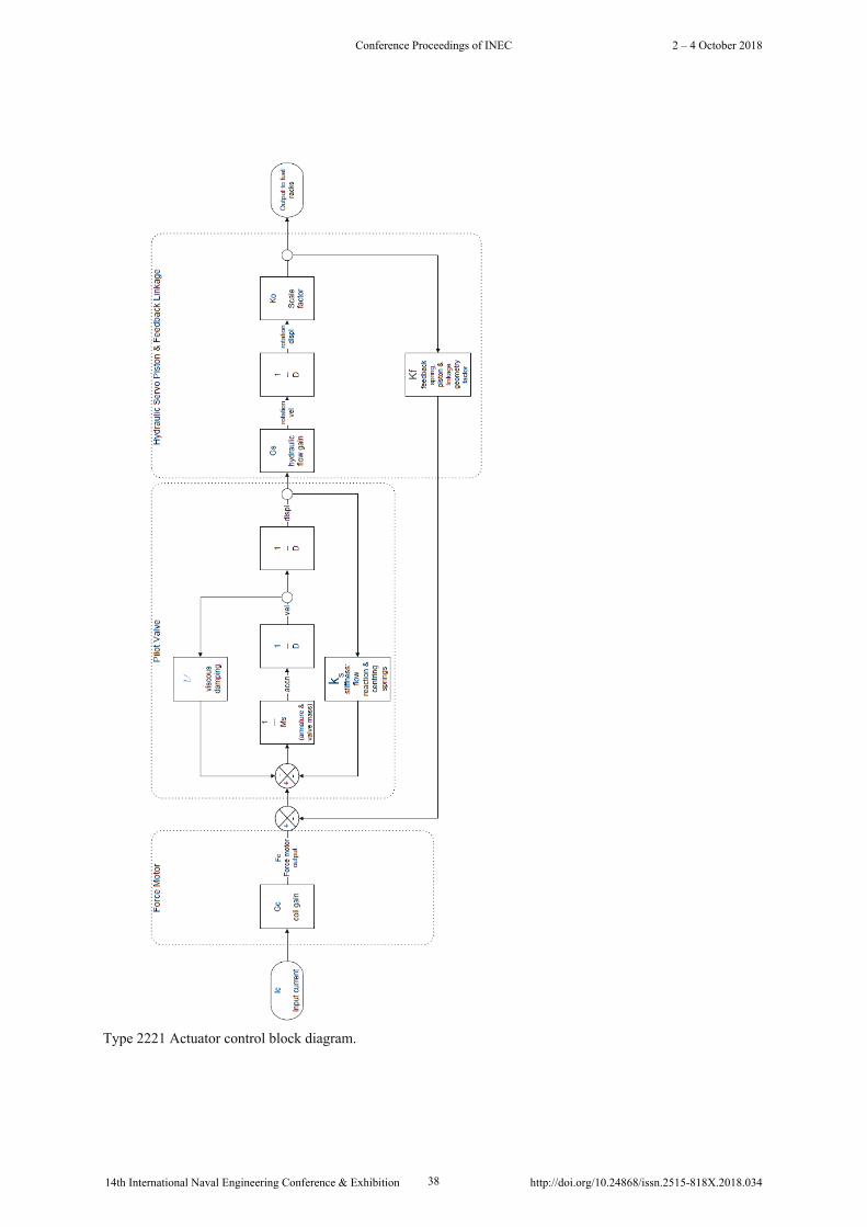
Type 2221 Actuator control block diagram.



Appendix 3

True 3 phase power generation and propulsion model in 20-sim. . This model has the ability to simulate the transients at parallel switching of the generators and the dynamics of active loadsharing between the generators. The other interesting possibilities of this model are the investigation of short circuit events, and with the package 20-sim 4C it opens the possibility to do HIL simulations.

From the 20 sim website: 20-sim 4C enables rapid prototyping for control engineers. With 20-sim 4C you can run c-code on hardware to control machines and systems.

Power generation model name : Parr_302date: 17-05-2018

sp_Ugenmv_Ugen

exc_onexc_off AVR

out

AVR_G1

sp_Ugenmv_Ugen

exc_onexc_off AVR

out

AVR_G2

Bus-TieControl

Bustie_sp

Bustie_sp1

0 1 0bustie_sync_cmd

0 1 0bustie_sync_cmd1

CB_control_G1

0 1 0CB_G1_close

0 1 0

CB_G1_open

Circuit_braker

Circuit_braker1

0 1 0cmd_CB_G2_CLOSE

0 cmd_CB_G2_CLOSE1

0 1 0cmd_CB_G2_open

0 cmd_CB_G2_open1

0 cmd_off_load_G1

0 1 0cmd_off_load_G2

0 1 0 cmd_start_sync_G1

0 1 0cmd_start_sync_G2

Constant

COUcoupling1

COUcoupling2

COU +CLUcoupling_clutch

COU +CLU

coupling_clutch1

Delay

on

off

2

Demux

0 1 0Dief_loadshare_cmd

0 1 0Dief_loadshare_cmd1

Engine

Diesel_1

Engine

Diesel_2

0 1 0DroopFalse

0 DroopFalse1

0 1 0

droop_on

0 droop_on1

0 1 0exc_off_G1

0 1 0exc_off_G2

0 1 0

exc_on_G1

0 1 0

exc_on_G2

K

fe2wn1

K

fe2wn2

freq

FreqBUS

freq

FreqGEN

SG

G1

SG

G2

K

Gearbox

Gearbox1

GOV

sp. speed

mv. gen shaft

droop-ondroop-off

fuel

Governor1

GOV

sp. speed

mv. gen shaft

droop-ondroop-off

fuel

Governor2

Load

Loadcontrol_P1

0 1 0Load_1_down

0 1 0Load_1_up

Load_33

Load_66

Load_ctrl

Load_Full

LoadShare

Load_share

LoadShare

Load_share1

Load_S_PF

Low-Pass FilterBW 2 (Hz) nd

LowPassFilter1


LowPassFilter2


LowPassFilter3


LowPassFilter4


LowPassFilter5


LowPassFilter6

LPFFO

1

Or

Or1

P

P

Pabc_G1

Pabc_G2

Global Holec 2

Parameters_calculation

P

P

P

P

K

percent_load

PF

PP

PP

pulse_off

Q_ctrl

Droop

ReactiveDroop

Droop

ReactiveDroop1

RefClutch

RefClutch1setpoint_U_G1

setpoint_U_G2

Sine

0 1 0speed_down_diesel

0 1 0speed_down_diesel1

Setpoint speed

cmd. stop

cmd. start

cmd. speed-up

cmd. speed-down

speed setpoint

load share on

sp. load share

sync. onsp. sync.

load-off

Bustie_sync_cmd

Bustie_sp

Dief_loadshare_cmd

VMS_loadshare_cmd

VMS_sp

droop_ondroop-off

Speed_ref_1

Setpoint speed

cmd. stop

cmd. start

cmd. speed-up

cmd. speed-down

speed setpoint

load share on

sp. load share

sync. onsp. sync.

load-off

Bustie_sync_cmd

Bustie_sp

Dief_loadshare_cmd

VMS_loadshare_cmd

VMS_sp

droop_ondroop-off

Speed_ref_2

0 1 0speed_up_diesel

0 1 0speed_up_diesel1

0 1 0start_diesel

0 1 0start_diesel1

0 1 0stop_diesel

0 1 0stop_diesel1

swtich

Synchronizer-1

Bus-Tie open cmd.Bus-Tie close cmd.

manual Bus-Tie close

Load share on

freq. G2sp. mech. freq.

sp. speed Gext Powersync. on load off

G PowerUa refUa G

manual Bus-Tie open

manual sync.

manual load off

Synchronizer_1

Synchronizer-2

Bus-Tie open cmd.Bus-Tie close cmd.

manual Bus-Tie close

Load share on

freq. G2sp. mech. freq.

sp. speed Gext Powersync. on load off

G PowerUa refUa G

manual Bus-Tie open

manual sync.

manual load off

Synchronizer_2

K

T1

K

T2

LPFFO

Torque_1

LPFFO

Torque_2

0 1 0VMS_loadshare_cmd

0 1 0VMS_loadshare_cmd1

VMS_sp

VMS_sp1

0

0

00

0



True 3 phase synchronous generator BG model in 20-sim. The model is based on the equations of Park, it is not easy to use this model because it uses generator parameters not easily available from the manufacturer.

-idid

-iq

iq

PU

RK4

@ 0

.001

Ld =

80e

-5;

Rd =

1e-

5;R

= 0.

1;C

= 20

00e-

6

iexc

iter

phas

e_a

phas

e_b

phas

e_c

Tm

Ua

Q

delta

_G1

delta

K Gain

Vnp

In

x yÐ|R

|

Ia_rms

IId

1 iD

1

K

iexc_to_if

1if_t

IIq

1 iQ

1

Limit

LPF

FO

LPF

FO

LPF

FO

LPF

FO

2

Mux

2

Mux1

TF Np

1

1M

TFPark1

phase

PhaseSensor

phase

PhaseSensor1

PQ _

iu

S

PQS_Sensor

MG

Ypsi_d

MG

Ypsi_q

pu2SI

pu2SI_a

pu2SI

pu2SI_b

pu2SI

pu2SI_c

pu2SI

pu2SI_T

Qabc_GEN

RRD

Remanence

RRf

R RQ

RRs R Rs1

SI2pu

SI2pu_f

-sin

Sine

theta

x yÐ|R

|

Va_rms

0

MSe Vf

00

0 0

0

0



Torsional Vibration Analysis by Bondgraph Modelling. A ...

Documents