Torsion in Helically Reinforced Prestressed Concrete Poles

Torsion in Helically Reinforced

Prestressed Concrete Poles

by

Michael Eduard Kuebler

A thesis

presented to the University of Waterloo

in fulfillment of the

thesis requirement for the degree of

Master of Applied Science

in

Civil Engineering

Waterloo, Ontario, Canada, 2008

©Michael Eduard Kuebler 2008

ISBN фтуπлπпфпπпотлпπф

ii

AUTHOR'S DECLARATION

I hereby declare that I am the sole author of this thesis. This is a true copy of the thesis, including any

required final revisions, as accepted by my examiners.

I understand that my thesis may be made electronically available to the public.

iii

Abstract

Reinforced concrete poles are commonly used as street lighting and electrical transmission poles.

Typical concrete lighting poles experience very little load due to torsion. The governing design loads

are typically bending moments as a result of wind on the arms, fixtures, and the pole itself. The

Canadian pole standard, CSA A14-07 relates the helical reinforcing to the torsion capacity of concrete

poles. This issue and the spacing of the helical reinforcing elements are investigated.

Based on the ultimate transverse loading classification system in the Canadian standard, the code

provides a table with empirically derived minimum helical reinforcing amounts that vary depending

on: 1) the pole class and 2) distance from the tip of the pole. Research into the minimum helical

reinforcing requirements in the Canadian code has determined that the values were chosen

empirically based on manufacturer’s testing. The CSA standard recommends two methods for the

placement of the helical reinforcing: either all the required helical reinforcing is wound in one

direction or an overlapping system is used where half of the required reinforcing is wound in each

direction. From a production standpoint, the process of placing and tying this helical steel is time

consuming and an improved method of reinforcement is desirable. Whether the double helix method

of placement produces stronger poles in torsion than the single helix method is unknown. The

objectives of the research are to analyze the Canadian code (CSA A14-07) requirements for minimum

helical reinforcement and determine if the Canadian requirements are adequate. The helical

reinforcement spacing requirements and the effect of spacing and direction of the helical reinforcing

on the torsional capacity of a pole is also analyzed. Double helix and single helix reinforcement

methods are compared to determine if there is a difference between the two methods of

reinforcement.

The Canadian pole standard (CSA A14-07) is analyzed and compared to the American and German

standards. It was determined that the complex Canadian code provides more conservative spacing

requirements than the American and German codes however the spacing requirements are based on

empirical results alone. The rationale behind the Canadian code requirements is unknown.

A testing program was developed to analyze the spacing requirements in the CSA A14-07 code.

Fourteen specimens were produced with different helical reinforcing amounts: no reinforcement,

single and double helical spaced CSA A14-07 designed reinforcement, and single helical specimens

with twice the designed spacing values. Two specimens were produced based on the single helical

iv

reinforcement spacing. One specimen was produced with helical reinforcement wound in the

clockwise direction and another with helical reinforcement in the counter clockwise direction. All

specimens were tested under a counter clockwise torsional load. The clockwise specimens

demonstrated the response of prestressed concrete poles with effective helical reinforcement whereas

the counter clockwise reinforced specimens represented theoretically ineffective reinforcement. Two

tip sizes were produced and tested: 165 mm and 210 mm.

A sudden, brittle failure was noted for all specimens tested. The helical reinforcement provided no

post-cracking ductility. It was determined that the spacing and direction of the helical reinforcement

had little effect on the torsional capacity of the pole. Variable and scattered test results were

observed. Predictions of the cracking torque based on the ACI 318-05, CSA A23.3-04 and Eurocode

2 all proved to be unconservative. Strut and tie modelling of the prestressing transfer zone suggested

that the spacing of the helical steel be 40 mm for the 165 mm specimens and 53 mm for the 210 mm

specimens. Based on the results of the strut and tie modelling, it is likely that the variability and

scatter in the test results is due to pre-cracking of the specimens. All the 165 mm specimens and the

large spaced 210 mm specimens were inadequately reinforced in the transfer zone. The degree of

pre-cracking in the specimen likely causes the torsional capacity of the pole to vary.

The strut and tie model results suggest that the requirements of the Canadian code can be simplified

and rationalized. Similar to the American spacing requirements of 25 mm in the prestressing transfer

zone, a spacing of 30 mm to 50 mm is recommended dependent on the pole tip size. Proper concrete

mixes, adequate concrete strengths, prestressing levels, and wall thickness should be emphasized in

the torsional CSA A14-07 design requirements since all have a large impact on the torsional capacity

of prestressed concrete poles.

Recommendations and future work are suggested to conclusively determine if direction and

spacing have an effect on torsional capacity or to determine the factors causing the scatter in the

results. The performance of prestressed concrete poles reinforced using the suggestions presented

should also be further investigated. Improving the ability to predict the cracking torque based on the

codes or reducing the scatter in the test results should also be studied.

v

Acknowledgements

The author would like to thank Mr. Ken Bowman, Mr. Terry Ridgway, and Mr. Doug Hirst for their

suggestions and technical assistance during the testing program.

Special thanks to Mr. Ron Ragwen, Mr. Uli Kuebler, and Sky Cast Inc. whose support during the

experimental testing made this research possible. Thanks also to Mr. Nick Lawler for his assistance

during testing.

The author would also like to thank his parents and friends for their support during the past two years.

A final thank you is extended to his supervisor, Professor Dr. Maria Anna Polak, P. Eng., whose

guidance and suggestions have been invaluable during this research.

vi

Table of Contents

List of Tables.......................................................................................................................................... x List of Figures ......................................................................................................................................xii Chapter 1 Introduction............................................................................................................................ 1

1.1 Background .................................................................................................................................. 1 1.1.1 Brief History of Prestressed Concrete Poles.......................................................................... 1 1.1.2 Typical Concrete Poles Failures ............................................................................................ 2

1.2 Justification and Scope of Research ............................................................................................. 5 1.3 Objectives..................................................................................................................................... 6 1.4 Contributions ................................................................................................................................ 6 1.5 Organization of Thesis ................................................................................................................. 7

Chapter 2 Literature Review .................................................................................................................. 8 2.1 Literature on Concrete Poles ........................................................................................................ 8

2.1.1 Field Behaviour of Prestressed Concrete Poles ..................................................................... 8 2.1.2 FRP and Prestressed Concrete Poles ..................................................................................... 9 2.1.3 Helical Reinforcement in Concrete Poles............................................................................ 11 2.1.4 Concrete Mixes for Spun-cast Concrete Poles .................................................................... 12 2.1.5 Published Guides and Specifications for Prestressed Concrete Pole Design ...................... 12

2.1.5.1 Guide Specification for Prestressed Concrete Poles..................................................... 12 2.1.5.2 Guide for Design of Prestressed Concrete Poles ..........................................................13 2.1.5.3 Guide for the Design and Use of Concrete Poles ......................................................... 14 2.1.5.4 Guide for the Design of Prestressed Concrete Poles (ASCE/PCI Joint Report) .......... 14

2.2 AASHTO and Canadian Highway Bridge Design Code Requirements for Concrete Poles ...... 16 2.2.1 AASHTO Standard Specifications for Structural Supports for Highway Signs, Luminaries,

and Traffic Signals ....................................................................................................................... 16 2.2.2 Canadian Highway Bridge Design Code............................................................................. 16

2.3 Design of Concrete Poles ........................................................................................................... 16 2.3.1 CSA A14 (Canadian Standard) ........................................................................................... 17 2.3.2 DIN EN 12843: Precast concrete products – Masts and poles and DIN EN 40-4: Lighting

Columns (German Standards) ...................................................................................................... 20

vii

2.3.3 ASTM Standard: Standard Specification for Spun Cast Prestressed Concrete Poles (U.S.A

Standard) ...................................................................................................................................... 21 2.3.4 Comparison of Helical Reinforcement Code Spacing Requirements.................................. 21

2.4 Torque Resistance Formulae ...................................................................................................... 23 2.4.1 Cracking Torque Resistance................................................................................................ 23 2.4.2 Ultimate Torsional Resistance............................................................................................. 29

2.5 Minimum Transverse Reinforcing Spacing................................................................................ 31 2.6 Torsion Models........................................................................................................................... 35

2.6.1 Mechanics of Torsion in Reinforced Concrete Members.................................................... 35 2.6.1.1 Equilibrium Conditions ................................................................................................ 36 2.6.1.2 Compatibility Conditions ............................................................................................. 37 2.6.1.3 Material Laws (Constitutive Conditions) ..................................................................... 39

2.6.2 Analytical Models for Torsion ............................................................................................ 41 2.6.2.1 Compression Field Theory “Spalled Model” ...............................................................41 2.6.2.2 Softened Truss Model................................................................................................... 43 2.6.2.3 Differences between the Compression Field Theory and Softened Truss Model ........ 45

Chapter 3 Analytical Models for Concrete Pole Design ...................................................................... 47 3.1 General Pole Design ................................................................................................................... 47 3.2 Pole Capacity Calculation Program............................................................................................ 48 3.3 Torsional Response Program using Analytical Models for Torsion .......................................... 55

3.3.1 Validation of the Torsional Response Program Output....................................................... 58 Chapter 4 Design of Test Program ....................................................................................................... 62

4.1 General ....................................................................................................................................... 62 4.2 Experimental Program................................................................................................................ 62 4.3 General Specimen Dimensions................................................................................................... 65 4.4 CSA A23.3-4 Specimen Design Moment, Shear and Torsion Values .......................................78 4.5 Specimen Preparation................................................................................................................. 79 4.6 Concrete Mix.............................................................................................................................. 82

4.6.1 Prestressing Strand .............................................................................................................. 83 4.6.2 Helical (Transverse) Reinforcement and Wall Thickness ................................................... 84 4.6.3 Curing Cycle........................................................................................................................ 86 4.6.4 Concrete Compressive and Tensile Strengths ..................................................................... 87

viii

Chapter 5 Experimental Setup and Procedures .................................................................................... 90 5.1 Test Setup and Apparatus........................................................................................................... 90 5.2 Instrumentation........................................................................................................................... 93

5.2.1 Data acquisition system....................................................................................................... 93 5.2.2 Load Cells and Single Channel Signal Conditioner ............................................................ 93 5.2.3 Electronic Clinometer.......................................................................................................... 95 5.2.4 Documentation Equipment .................................................................................................. 97

5.3 Testing Procedures ..................................................................................................................... 97 Chapter 6 Experimental Results ........................................................................................................... 99

6.1 Test Observations ....................................................................................................................... 99 6.1.1 Test Observations for 210 mm Tip Specimens ................................................................. 100

6.1.1.1 Specimen 210-C .........................................................................................................100 6.1.1.2 Specimen 210-C-2 ...................................................................................................... 105 6.1.1.3 Specimen 210-D .........................................................................................................105 6.1.1.4 Specimen 210-CCW-L ............................................................................................... 109 6.1.1.5 Specimen 210-CW-L.................................................................................................. 111 6.1.1.6 Specimen 210-CCW-N............................................................................................... 111 6.1.1.7 Specimen 210-CW-N ................................................................................................. 115

6.1.2 Test Observations for 165 mm Tip Specimens ................................................................. 117 6.1.2.1 Specimen 165-C .........................................................................................................117 6.1.2.2 Specimen 165-C-2 ...................................................................................................... 119 6.1.2.3 Specimen 165-D .........................................................................................................122 6.1.2.4 Specimen 165-CCW-L ............................................................................................... 122 6.1.2.5 Specimen 165-CW-L.................................................................................................. 126 6.1.2.6 Specimen 165-CW-N ................................................................................................. 126 6.1.2.7 Specimen 165-CCW-N............................................................................................... 130

Chapter 7 Analysis of Experimental Results...................................................................................... 132 7.1 General Experimental Results .................................................................................................. 132 7.2 Graphical Experimental Results Comparison........................................................................... 133

7.2.1 Cracking Torque Comparison ........................................................................................... 133 7.2.2 Influence of Diameter and Wall Thickness on Torsional Capacity................................... 134 7.2.3 Stiffness Difference between 165 and 210 Specimens...................................................... 134

ix

7.2.4 Helical Reinforcing Direction ........................................................................................... 138 7.2.5 Helical Reinforcing Spacing.............................................................................................. 140 7.2.6 Analysis of Failure Location (Clamp vs. Collar Failure) .................................................. 141

7.3 Comparison of Softened Truss and Spalled Models to Test Results........................................ 144 7.4 Minimum Transverse Reinforcement Requirements................................................................ 149

7.4.1 Prestressing Transfer Zone Strut and Tie Model............................................................... 149 7.4.2 Code Required Maximum Transverse Reinforcement Spacing ........................................ 152

7.5 Comparison of Experimental and Theoretical Cracking Torque Results .................................153 7.6 Factors Affecting Theoretical Cracking Torque Formulae ...................................................... 161 7.7 Influence of Longitudinal Cracking, Segregation, and Concrete Quality on Cracking Torque162 7.8 Discussion on the Variation in the Results ............................................................................... 165

7.8.1 Sky Cast Inc. Database and Experimental Specimen Comparison.................................... 165 7.8.2 Experimental Variation and the CSA A14-07 Spacing Provisions ................................... 170

7.9 Economic Analysis of Helical Reinforcing ..............................................................................173 7.10 Analysis and Comparison of Typical Applied Torques on Lighting Poles ............................ 174

Chapter 8 Conclusions and Recommendations for Future Work ....................................................... 177 References .......................................................................................................................................... 180

Appendices

Appendix A Pole Analysis Output for Design of Specimen .......................................................... 185

Appendix B Specimen Material Reports........................................................................................ 192

Appendix C Testing Raw Data Sheets ........................................................................................... 222

Appendix D Strut and Tie Model and Code Maximum Spacing Calculations .............................. 238

Appendix E Typical Fixture Product Sheets and Wind Load Calculations ................................... 243

x

List of Tables

Table 2-1: Minimum Ultimate Transverse Capacity (CSA A14-07 Table 1) .................................... 18 Table 2-2: Minimum Amounts of Helical Reinforcing (CSA A14-07 Table 2) ................................ 18 Table 2-3: Minimum Torsional Capacities (CSA A14-07 Table 3) .................................................... 18 Table 2-4: DIN 4228 (1989): Helical steel spacing requirements....................................................... 20 Table 2-5: Helical reinforcement spacing code comparison ............................................................... 23 Table 2-6: Summary of Variables and Equations for Torsion (Hsu, 1988)......................................... 35 Table 4-1: Summary of experimental program ................................................................................... 64 Table 4-2: Specimen description ......................................................................................................... 64 Table 4-3: Specimen design dimensions and classification ................................................................ 65 Table 4-4: Calculated unfactored 165 and 210 specimen moment, shear, and torsional capacities....78 Table 4-5: Calculated factored 165 and 210 specimen moment, shear, and torsional capacities........78 Table 4-6: Summary of target mix and actual specimen concrete mixes ............................................ 83 Table 4-7: Summary of prestressing strand strains and stress values.................................................. 84 Table 4-8: Target helical reinforcing spacing/percentages and concrete wall thickness..................... 85 Table 4-9: Actual helical reinforcing spacing/percentages and concrete wall thickness .................... 85 Table 4-10: Summary of concrete cylinder compressive and tensile strengths................................... 88 Table 6-1: Summary of initial test excitation and calibration readings............................................... 99 Table 6-2: Summary of 210 mm tip Experimental Results ............................................................... 101 Table 6-3: Summary of 165 mm tip Experimental Results ............................................................... 102 Table 7-1: Comparison of average stiffness for 165 and 2 10 specimens ......................................... 135 Table 7-2: Strut and tie transfer zone model spacing results............................................................. 151 Table 7-3: Comparison of experimental and theoretical cracking torque results (at 0.6 m and using

measured prestressing) ............................................................................................................... 154 Table 7-4: Comparison of experimental and theoretical cracking torque results (at failure location

and using measured prestressing) ............................................................................................... 155 Table 7-5: Comparison of experimental and theoretical cracking torque results (at 0.6 m and using

assumed prestressing)................................................................................................................. 156 Table 7-6: Comparison of experimental and theoretical cracking torque results (at failure location

and using assumed prestressing) ................................................................................................ 157

xi

Table 7-7: Comparison of ACI-318-05 Statistical Data with and without control specimens .......... 161 Table 7-8: Comparison between strut and tie spacing requirements and specimen spacing.............173 Table 7-9: Savings due to helical spacing changes ........................................................................... 173

xii

List of Figures

Figure 1.1: Shear failure caused by vehicle impact (Sky Cast, 2008) ................................................... 3 Figure 1.2 a) and b): Pole failure caused by vehicle impact and inertia effects (Sky Cast Inc., 2007) .4 Figure 1.3 a) and b): Longitudinal cracking, corrosion and spalling caused by differential shrinkage

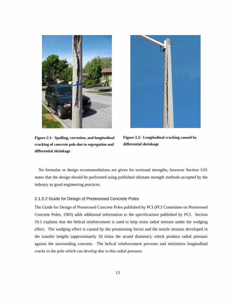
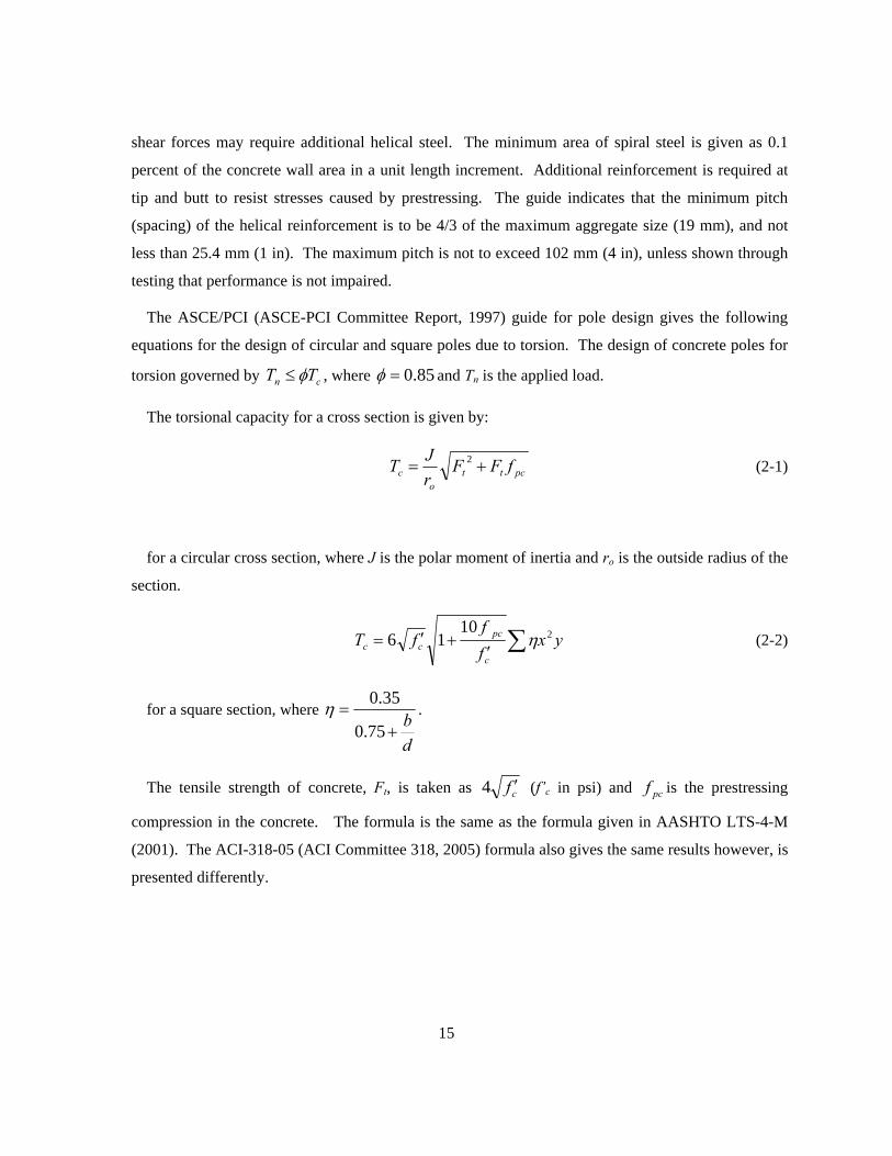
and segregation of concrete mix..................................................................................................... 5 Figure 2.1: Spalling, corrosion, and longitudinal cracking of concrete pole due to segregation and

differential shrinkage.................................................................................................................... 13 Figure 2.2: Longitudinal cracking caused by differential shrinkage ................................................... 13 Figure 2.3: Derivation of helical reinforcement spacing formula for hollow tapered concrete poles .21 Figure 2.4: Helical spacing versus wall thickness for CSA A14-07, ASTM C 1089-06 and DIN EN

12843 ............................................................................................................................................ 22 Figure 2.5: Bredt's "thin-tube" theory (ACI Committee 445, 2006) ................................................... 24 Figure 2.6: Derivation of prestressing factor (ACI Committee 445, 2006)......................................... 25 Figure 2.7: Rausch's space truss model (ACI Committee 445, 2006) ................................................. 30 Figure 2.8: Coordinate systems and variable definition (ACI Committee 445, 2006)........................ 36 Figure 2.9: Warping of member wall section (Collins and Mitchell, 1974)........................................38 Figure 2.10: Strain and Stress Distribution in Concrete Struts (ACI Committee 445, 2006) ............. 39 Figure 2.11: Softened stress-strain curve for concrete (Pang and Hsu, 1996) .................................... 39 Figure 2.12: Spalling of Concrete Cover (ACI Committee 445, 2006)............................................... 42 Figure 2.13: Compression Field Theory Shear Flow (ACI Committee 445, 2006) ............................ 42 Figure 2.14: Softened Truss Model Stress Distribution (ACI Committee 445, 2006) ........................ 44 Figure 3.1: Calculation of pole concrete compression area................................................................. 47 Figure 3.2: Rotated geometry of prestressing strands ......................................................................... 48 Figure 3.3: Flowchart of Pole Capacity Calculation Program............................................................. 49 Figure 3.4: Screenshot of Pole Capacity Calculation Program ........................................................... 50 Figure 3.5: Diagram of layered parabolic stress-strain analysis..........................................................52 Figure 3.6: Moment resistance output from pole program.................................................................. 53 Figure 3.7: Shear resistance output from pole program ...................................................................... 54 Figure 3.8: Torsional resistance output from pole program ................................................................ 54 Figure 3.9: Flowchart of the Softened Truss Model Program............................................................. 56

xiii

Figure 3.10: Flowchart of the Compression Field Theory (spalled model) program.......................... 57 Figure 3.11: Box section example details (Hsu, 1991b)...................................................................... 58 Figure 3.12: Comparison of Softened Truss Model example (Hsu, 1991) and Torsional Response

program output ............................................................................................................................. 59 Figure 3.13: Comparison of McMullen and El-Degwy (1985) specimen PB1 results and Torsional

Response program output ............................................................................................................. 60 Figure 3.14: Comparison of McMullen and El-Degwy (1985) specimen PB4 results and Torsional

Response program output ............................................................................................................. 61 Figure 4.1: Example helical reinforcing layouts a) 165-CW-N, b) 165-CCW-L c) 210-D d) 210-

CCW-N......................................................................................................................................... 63 Figure 4.2: 165 Control Specimen (165-C) ......................................................................................... 66 Figure 4.3: 165 Double Helix Specimen (165-D) ............................................................................... 67 Figure 4.4: 165 Single CW Helix Large Spaced Specimen (165-CW-L) ........................................... 68 Figure 4.5: 165 Single CCW Helix Large Spaced Specimen (165-CCW-L) ......................................69 Figure 4.6: 165 Single CW Helix Normal Spaced Specimen (165-CW-N) ........................................ 70 Figure 4.7: 165 Single CCW Helix Normal Spaced Specimen (165-CCW-N)................................... 71 Figure 4.8: 210 Control Specimen (210-C) ......................................................................................... 72 Figure 4.9: 210 Double Helix Specimen (210-D) ............................................................................... 73 Figure 4.10: 210 Single CW Helix Large Spaced Specimen (210-CW-L) ......................................... 74 Figure 4.11: 210 Single CCW Helix Large Spaced Specimen (210-CCW-L) .................................... 75 Figure 4.12: 210 Single CW Helix Normal Spaced Specimen (210-CW-N) ...................................... 76 Figure 4.13: 210 Single CCW Helix Normal Spaced Specimen (210-CCW-N)................................. 77 Figure 4.14: Placing the helical reinforcing ........................................................................................ 80 Figure 4.15: Spacing the helical reinforcing ....................................................................................... 80 Figure 4.16: Pouring and placing of concrete...................................................................................... 81 Figure 4.17: Tightening bolts on mould .............................................................................................. 81 Figure 4.18: Mould on spinning machine............................................................................................ 81 Figure 4.19: Kiln and curing process .................................................................................................. 81 Figure 4.20: De-moulding machine..................................................................................................... 81 Figure 4.21: Releasing pole from mould ............................................................................................. 81 Figure 4.22: Typical prestressed concrete steam curing cylcle .......................................................... 87 Figure 4.23: Specimen compression strength development to time of testing ................................... 88

xiv

Figure 5.1: Test bed layout and test setup ........................................................................................... 91 Figure 5.2 a) - e): Pictures of test setup............................................................................................... 92 Figure 5.3: Signal conditioner with voltage divider ............................................................................ 94 Figure 5.4: Load cell calibration 1 ...................................................................................................... 96 Figure 5.5: Load cell calibration 2 (with voltage divider)................................................................... 96 Figure 5.6: Diagram of cracking patterns, failure locations, and loading terminology....................... 97 Figure 6.1: a) – f) 210-C test observation photos .............................................................................. 103 Figure 6.2: Torque-twist history for 210-C ....................................................................................... 104 Figure 6.3: Torque-twist history for 210-C-2.................................................................................... 104 Figure 6.4: a) – e) 210-C-2 test observation photos .......................................................................... 106 Figure 6.5: a) – e) 210-D test observation photos ............................................................................. 107 Figure 6.6: Torque-twist history for 210-D....................................................................................... 108 Figure 6.7: Torque-twist history for 210-CCW-L ............................................................................. 108 Figure 6.8: a) – f) 210-CCW-L test observation photos....................................................................110 Figure 6.9: a) – f) 210-CW-L test observation photos ......................................................................112 Figure 6.10: a) – e) 210-CCW-N test observation photos ................................................................. 113 Figure 6.11: Torque-twist history for 210-CW-L.............................................................................. 114 Figure 6.12: Torque-twist history for 210-CCW-N........................................................................... 114 Figure 6.13: a) – e) 210-CW-N test observation photos.................................................................... 116 Figure 6.14: Torque-twist history for 210-CW-N ............................................................................. 117 Figure 6.15: a) – f) 165-C test observation photos ............................................................................ 118 Figure 6.16: Torque-twist history for 165-C ..................................................................................... 119 Figure 6.17: a) – f) 165-C-2 test observation photos......................................................................... 120 Figure 6.18: Torque-twist history for 165-C-2.................................................................................. 121 Figure 6.19: Specimen 165-C-2 load history without collar slip....................................................... 121 Figure 6.20: a) – f) 165-D test observation photos............................................................................ 123 Figure 6.21: a) – e) 165-CCW-L test observation photos ................................................................. 124 Figure 6.22: Torque-twist history for 165-D..................................................................................... 125 Figure 6.23: Torque-twist history for 165-CCW-L........................................................................... 125 Figure 6.24: a) – f) 165-CW-L test observation photos ....................................................................127 Figure 6.25: Torque-twist history for 165-CW-L.............................................................................. 128 Figure 6.26: Torque-twist history for 165-CW-N ............................................................................. 128

xv

Figure 6.27: a) – d) 165-CW-N test observation photos ................................................................... 129 Figure 6.28: Torque-twist history for 165-CCW-N........................................................................... 130 Figure 6.29: a) – d) 165-CCW-N test observation photos................................................................. 131 Figure 7.1: Torque-twist history of 165 specimens...........................................................................133 Figure 7.2: Torque-twist history of 210 specimens...........................................................................133 Figure 7.3: Torque-twist response of 165 mm specimens................................................................. 134 Figure 7.4: Torque-twist response of 210 mm Specimens ................................................................ 134 Figure 7.5: 210 vs. 165 mm tip cracking torques .............................................................................. 135 Figure 7.6: Torque-twist curves for all specimens ............................................................................ 136 Figure 7.7: Linear portion of specimen results.................................................................................. 136 Figure 7.8: Linear elastic torsional predicted response compared to test results .............................. 137 Figure 7.9: 165 mm clockwise reinforced specimens ....................................................................... 139 Figure 7.10: 165 mm counter clockwise reinforced specimens ........................................................ 139 Figure 7.11: 210 mm clockwise reinforced specimens ..................................................................... 139 Figure 7.12: 210 mm counter clockwise reinforced specimens ........................................................ 139 Figure 7.13: Comparison between 165 mm clockwise and counter clockwise specimens ............... 140 Figure 7.14: Comparison between 210 mm clockwise and counter clockwise specimens ............... 140 Figure 7.15: 165 mm large spaced specimens (-L) ........................................................................... 142 Figure 7.16: 165 mm normal spaced specimens (-N)........................................................................ 142 Figure 7.17: 210 mm large spaced specimens (-L) ........................................................................... 142 Figure 7.18: 210 mm normal spaced specimens (-N)........................................................................ 142 Figure 7.19: Clamp failures for 165 mm specimens ......................................................................... 144 Figure 7.20: Collar failures of 165 mm specimens ........................................................................... 144 Figure 7.21: Clamp failures for 210 mm specimens ......................................................................... 144 Figure 7.22: Collar failures for 210 mm specimens .......................................................................... 144 Figure 7.23: Comparison between 165-N and 165-D specimens and torsion models....................... 146 Figure 7.24: Comparison between 165-L and 165–D specimens and torsion models ...................... 147 Figure 7.25: Comparison between 210-N and 210-D specimens and torsion models....................... 147 Figure 7.26: Comparison between 210-L and 210-D specimens and torsion models ....................... 148 Figure 7.27: Strut and tie model ........................................................................................................ 149 Figure 7.28: Strut and tie model for transfer length zone.................................................................. 150 Figure 7.29: Variation and accuracy of ACI 318-05 code predictions............................................. 158

xvi

Figure 7.30: Variation and accuracy of CSA A23.3-04 code predictions ......................................... 158 Figure 7.31: Variation and accuracy of EC2 code predictions.......................................................... 159 Figure 7.32: Effects of wall thickness, compressive strength, and prestressing stress on cracking

torque.......................................................................................................................................... 162 Figure 7.33: Longitudinal cracking (a) and strand slip (b) due to prestressing (165-C) ................... 163 Figure 7.34 a)-c): a) Typical paste wedge and segregation along inner wall of specimens b)

segregation of 210-CCW-L specimen c) extreme example from Chahrour and Soudki (2006)

pole testing ................................................................................................................................. 164 Figure 7.35: Sky Cast Inc. Torsion Database Results - 150 mm tip, 3/8" prestressing strand .......... 166 Figure 7.36: Sky Cast Inc. Torsion Database Results - 165 mm tip, 7/16" prestressing strand ........ 166 Figure 7.37: Sky Cast Inc. Torsion Database Results - 165 mm tip, 1/2" prestressing strand .......... 168 Figure 7.38: Sky Cast Inc. Torsion Database and Experimental Results - 165 mm tip, 3/8"strand ..168 Figure 7.39: Sky Cast Inc. Torsion Database and Experimental Results - 210 mm tip .................... 170 Figure 7.40: 165 mm specimens designed to CSA A14.................................................................... 171 Figure 7.41: 165 mm specimens against CSA A14........................................................................... 171 Figure 7.42: 210 mm specimens designed to CSA A14.................................................................... 171 Figure 7.43: 210 mm specimens against CSA A14........................................................................... 171 Figure 7.44: Applied factored torque versus 165 cracking torques................................................... 176 Figure 7.45: Applied factored torque versus 210 cracking torques................................................... 176

1

Chapter 1 Introduction

1.1 Background

1.1.1 Brief History of Prestressed Concrete Poles

Concrete poles have been used since the invention of reinforced concrete. In their paper titled “Spun

Prestressed Concrete Poles – Past, Present, and Future”, Fouad, Sherman and Werner (1992) present a

summary of the past 150 years of concrete poles. According to Fouad et al. the first concrete poles

were used in Germany in 1856 for supporting telegraph lines. In 1867, Joseph Monier of France

produced the first iron-reinforced concrete poles. The concrete poles had increased strength and

durability but usage was limited due to the heavier weight when compared to wood and steel. The

first spun cast concrete poles were first produced in 1907, by a German firm Otto Schlosser in

Meissen, northwest of Dresden. The result of the spinning process was a lighter pole due to the

hollow section. Since concrete poles were considered maintenance-free, by 1932, 250,000 poles were

in use in Europe, 150,000 in Germany only. Fouad et al. indicate that several poles built in the first

quarter of the 20th century are still in use today. For example, a 19 m high pole in Newmarkt,

Germany was built in 1924 with a 280 mm tip diameter, 50 MPa concrete, 18 to 20 mm diameter

longitudinal steel and 5 mm circumferential spiral wire at a spacing of 80 to 100 mm.

Eugene Freyssinet developed the first prestressed concrete poles during the 1930’s and produced

poles that could withstand higher loads without cracking and exhibited elastic characteristics. World

War II and the shortage of steel after the war increased the use of prestressed concrete poles since less

steel was required for production compared to conventional reinforced concrete poles. By the 1950’s

the first spun cast prestressed concrete poles were in production in Europe. The poles had improved

strength, durability, and were lighter when compared with other products. The result was that

transportation and erection was simplified. On the North American continent, reinforced concrete

poles were not used until the 1930’s. Prestressed poles were not used until the middle of the 1950’s

in the United States and became more common when the Virginia Electric Power Company (VEPCO)

and Bayshore Concrete Products started to produce efficient European designs of tapered spun

prestressed concrete poles (Fouad et al., 1992).

2

Fouad et al. also presented the advantages of concrete poles over steel and wood poles. Steel poles

normally cost more and require longer delivery times. Large wood poles on the other hand are

becoming scarce and expensive due to heavy forest cutting, fire, drought and disease. Fouad et al.

(1992) stated that “4 to 6 million wood poles become defective each year mainly due to rot and attack

by insects and woodpeckers.” In contrast, properly built prestressed concrete poles offer a somewhat

elastic, corrosion resistant, maintenance-free, and long lasting aesthetic product. Fouad et al. (1992)

suggest that while concrete poles are initially more expensive than wood poles, a life-cycle cost

analysis provides economic advantages due to the longer life span and reduced maintenance costs

associated with concrete poles.

A wide range of spun concrete poles can be produced, ranging from 6 m long, 200 mm base

diameter poles to 100 m long, 2 m base diameter poles (Fouad et al., 1992). Concrete poles can be

used in a variety of applications, including street lighting, electrical distribution, rail electrification,

communication towers, supports for wind turbines and several pole sections can be joined together to

produce 100 m long post-tensioned towers for communication equipment (Fouad et al., 1992). The

use of concrete poles has spread throughout Europe and North America and has become a popular

alternative to wood and steel poles.

1.1.2 Typical Concrete Poles Failures

The governing design loads are typically due to wind on the pole, arms, and fixtures. These loads

primarily produce bending moments, but also shear forces, and torsional moments. While failures

caused by overloads of moment, shear, and torsion are possible, very few have been documented and

no photos could be found. A few of the documented cases of concrete pole failures found by the

author are presented.

During the course of the thesis research two or three poles failed in the City of Kitchener in June of

2007. A storm caused high winds in the area and caused several trees and branches to fall all over

town. On Glasgow Street, falling branches landed on electrical lines causing the prestressed concrete

poles to fall over. While no known investigation was completed and very little information was

available to the author, it appeared from the pieces found that segregation of the concrete had

occurred during production. It is the author’s opinion that perhaps the sudden forces on the electrical

lines caused the inner cement paste to crack and spall causing the prestressing strands to break into

3

the hollow middle section of the pole. The loss of the strands could cause the pole to lose all

resistance and stability leading to the premature failure of the pole.

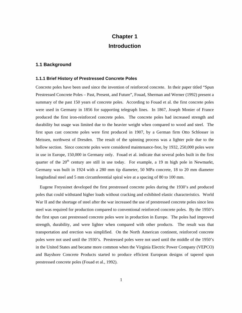
Vehicle impacts typically cause shear failure of concrete poles between the bumper level and the

ground (Dilger and Ghali, 1986). A typical shear failure caused by vehicle impact is shown in Figure

1.1. The crack caused by vehicle impact originates at the bumper level and proceeds diagonally

towards the ground level. As described by Dilger and Ghali (1986), disintegration of the surrounding

concrete occurs and may cause the pole to ultimately fall over. The use of tight spirals can minimize

the damaged area of the pole, while longitudinal reinforcement will provide the pole stability in the

case of complete concrete section loss.

Figure 1.1: Shear failure caused by vehicle impact (Sky Cast, 2008)

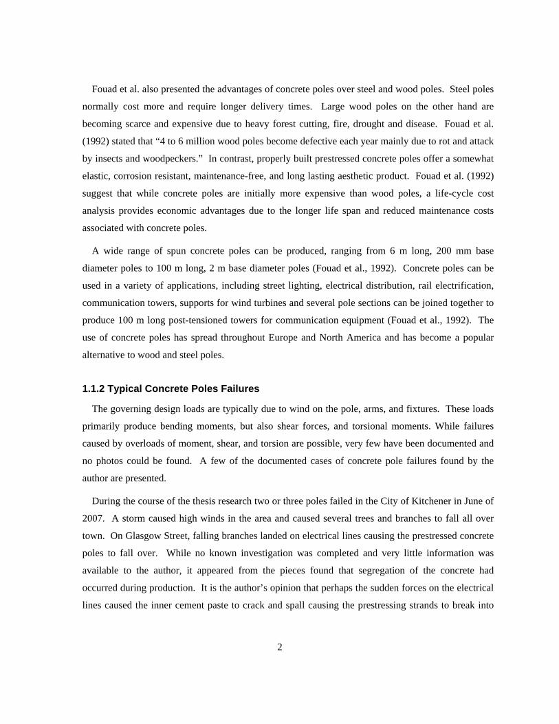
Damage and failure caused by vehicle impact is not always limited to the bumper level and

surrounding area. Improper embedment and vehicle impact forces can also cause failure to occur

below the ground. Inertia forces on the upper portion of the pole due to the vehicle impact can

alternatively cause the pole to snap higher up (Dilger and Ghali, 1986). Figure 1.2 shows an

architectural pole failure due to a vehicle impact. The failure of this pole occurred in two places. On

impact, cracking occurred below the ground where openings in the pole were made for electrical

4

wiring. Poles are typically reinforced with crash cages at points where vehicle collisions are possible.

Crash cages are made from conventional longitudinal steel reinforcement and tied together with

helical steel cages. Due to the sudden load on the pole and inertia forces (whiplash effect caused by

the collision), the upper portion of the pole shown in Figure 1.2 broke where the crash cage

longitudinal steel was terminated.

a) b)

Figure 1.2 a) and b): Pole failure caused by vehicle impact and inertia effects (Sky Cast Inc., 2007)

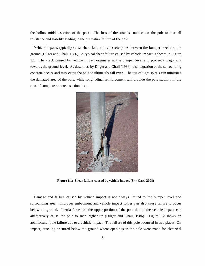
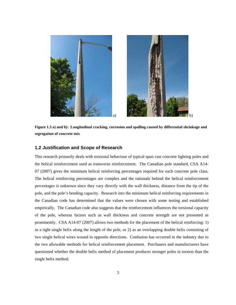
Another failure typically found in concrete poles and linked to segregation of the concrete and poor

concrete mixtures is shown in Figure 1.3. Segregation of the concrete during production of the

concrete poles creates several durability problems. Segregation creates a layer of fines and cement

paste along the inner surface of the wall. Differential shrinkage between the fine layer along the

inside of the pole and coarser layer on the outside of the pole can cause longitudinal cracks to develop

in the weaker cement paste layer (Dilger et al, 1996). Water infiltration then causes rusting of the

steel reinforcement leading to corrosion issues and increase cracking and spalling of the concrete.

5

a) b)

Figure 1.3 a) and b): Longitudinal cracking, corrosion and spalling caused by differential shrinkage and

segregation of concrete mix

1.2 Justification and Scope of Research

This research primarily deals with torsional behaviour of typical spun cast concrete lighting poles and

the helical reinforcement used as transverse reinforcement. The Canadian pole standard, CSA A14-

07 (2007) gives the minimum helical reinforcing percentages required for each concrete pole class.

The helical reinforcing percentages are complex and the rationale behind the helical reinforcement

percentages is unknown since they vary directly with the wall thickness, distance from the tip of the

pole, and the pole’s bending capacity. Research into the minimum helical reinforcing requirements in

the Canadian code has determined that the values were chosen with some testing and established

empirically. The Canadian code also suggests that the reinforcement influences the torsional capacity

of the pole, whereas factors such as wall thickness and concrete strength are not presented as

prominently. CSA A14-07 (2007) allows two methods for the placement of the helical reinforcing: 1)

as a tight single helix along the length of the pole, or 2) as an overlapping double helix consisting of

two single helical wires wound in opposite directions. Confusion has occurred in the industry due to

the two allowable methods for helical reinforcement placement. Purchasers and manufacturers have

questioned whether the double helix method of placement produces stronger poles in torsion than the

single helix method.

6

A deeper understanding of the reason for helical reinforcement placement in prestressed concrete

poles is needed for the simplification and rationalization of the CSA A14-07 minimum helical

reinforcing requirements. The purpose of the helical reinforcing steel, how much is required, and

whether the direction and/or spacing of the steel influences the torsional capacity of the concrete pole

must be determined to properly understand the helical reinforcing problem.

The research scope is limited to lighting and hydro poles where torsional loads are relatively small

and bending or shear typically govern the design. Where torsional loads are large and govern the

design, poles must be designed accordingly. Poles governed by large torsional loads are not part of

this research.

1.3 Objectives

The objectives of this research are to:

• Analyze the Canadian code (CSA A14-07) requirements for minimum helical reinforcement

and determine whether the requirements are adequate and,

• Determine the role of the helical steel reinforcement in sustaining torsional loads.

The research objectives are completed by: researching the development of the spacing requirements

for helical reinforcement in prestressed concrete poles, comparing the Canadian requirements against

pole codes from other countries, establishing whether spacing and direction (winding) of the helical

reinforcing has an effect on the torsional capacity of a pole, determining the difference between the

double helix and single helix reinforcement methods allowed by the Canadian code, and by

analyzing, through full scale testing, the mode of failure, post-cracking behaviour, and reason for

inclusion of helical reinforcement in prestressed concrete poles to determine the main factors that

influence the torsional capacity of prestressed concrete poles.

1.4 Contributions

The thesis summarizes current manufacturing and design practices for prestressed concrete poles.

The thesis gives a summary of concrete pole codes and literature and also provides a comparison

between the Canadian requirements for the design of prestressed concrete poles and the American and

German requirements.

7

A pole analysis program created as part of the research simplifies the design and analysis of

prestressed concrete poles and provides clear graphical output to the designer. Rational and simple

requirements are also presented for the design of helical reinforcing steel and the purpose for helical

steel in prestressed concrete poles is clarified.

1.5 Organization of Thesis

The remaining portion of the thesis is separated into six chapters. First a literature review (Chapter 2)

of concrete pole research, governing pole and concrete codes, and models for torsional response of

concrete members are presented. The cracking torque equations are derived and variations found in

the literature discussed. The mechanics and governing equations for the post-cracking torsion models

are also presented.

A MatLab program created for the flexural, shear, and torsional analysis of prestressed concrete

poles is presented in Chapter 3. Two other programs created to model the post-cracking torsional

behaviour of concrete poles are also discussed. Flowcharts and the program logic are presented and

validation/comparison of the output to existing data is given.

Chapter 4 summarizes the experimental testing program conducted and design of the specimens.

The design of the experimental specimens including the concrete mix/strength, prestressing strand,

helical reinforcement is discussed and the general spun cast production sequence is presented and

explained. The experimental test setup and instrumentation, and the testing procedure used are given

in Chapter 5. The experimental results and observations are summarized for each specimen in

Chapter 6. Pictures of the failure for each specimen and general remarks on each test are presented.

Chapter 7 contains an analysis of the experimental results. The chapter includes discussion on the

influence of helical reinforcing direction and spacing as well as concrete quality. A comparison of

the predicted cracking torques and torsional model behaviours to the experimental results is presented

and discussed. Factors important to the cracking torque of prestressed concrete poles are analyzed.

Comparison of the experimental data to a database of torsional pole testing results is also presented.

Finally an investigation into the applied loads on lighting poles and minimum transverse

reinforcement requirements in the prestressing transfer zone and the remaining portion of the pole is

discussed. The conclusions and recommendations are presented in Chapter 8. Appendices are also

attached which contain material reports and more detailed analysis and testing information.

8

Chapter 2 Literature Review

2.1 Literature on Concrete Poles

Publications and papers related to concrete poles and prestressed concrete poles generally fall into the

following categories: analysis techniques (typically bending capacity), concrete mixtures (durability

and performance), construction techniques, and impact/bending testing. Only a few papers discussed

helical reinforcing and the reasoning for placing it. None mentioned how spacing requirements were

developed for concrete poles while only one paper dealt with the combined bending and torsional

capacity of prestressed concrete poles. The following sections summarize the findings of the papers

dealing with concrete poles.

2.1.1 Field Behaviour of Prestressed Concrete Poles

Fouad et al. (1994) studied the performance of spun prestressed concrete poles during Hurricane

Andrew in Dade County, Florida. Hurricane Andrew was a category 4 hurricane with wind speeds in

the range of 211 to 249 km/h (131 to 155 mph). Fouad et al. inspected poles in Dade Country and

found they were in good structural condition even though cracking and near ultimate strength loads

had been applied. The poles were able to dissipate energy and survive the storm due to an inherent

ductility achieved through partial prestressing and a round cross section. The cracks formed due to

the hurricane appeared to fully close, indicating no yielding of prestressing steel and that the elasticity

was maintained. Full-scale bending tests were performed on six poles subjected to the hurricane

winds and it was determined that the storm did not cause a reduction in the strength of the poles. In

fact, the poles failed at loads 8 and 32 percent greater than the theoretical ultimate design capacity.

Fouad et al. suggested that the improved performance could be attributed to the high compaction

forces applied to the concrete in the spinning process. The result is a much denser concrete with

reduced water-cement ratio and improved material properties. Fouad et al. indicated that a modulus

of elasticity 28 percent larger than cast concrete can be achieved through spinning of the concrete. It

was noted that the failure rate for all concrete poles (both prestressed and static cast) during Hurricane

Andrew was 8 percent as compared to 80 percent for wood poles in the same area. The 8 percent of

9

concrete pole failures were all statically-cast square poles while no failures of spun-cast round poles

were reported.

The behaviour and design of static cast prestressed concrete poles were studied by Rosson et al.

(1996). Two full-scale poles were tested as prototypes to test the design methodology suggested in

the paper. Two poles were tested in bending, one constructed with helical steel (No. 9 gauge/2.9 mm

diameter spaced at 152 mm) and the other without. The mix used consisted of 318 kg of cement, 159

kg of Class C fly ash, 500 kg of masonry sand, 750 kg of 13 mm limestone, 136 kg of water, and 5.3

L of Rheobuild. The corresponding water-cement ratio was 0.43 and slump was measured as 203

mm.

During testing, the cracks due to bending were closed after release of the load showing that

corrosion of steel due to cracked concrete is prevented due to prestressing. The pole without spiral

reinforcement failed at a higher load than the one with spiral reinforcement. The pole with spiral

reinforcement failed in compression at the ground line and failure was confined due to the spiral

reinforcement. The second pole tested without spiral reinforcement failed due to a combination of

unconfined longitudinal cracking between prestressing strands and crushing at the ground line.

The shear strength provided by the concrete was deemed adequate to resist the design shear forces

and therefore shear reinforcement provided by the helical steel was not required. Rosson et al.

suggested however, that spiral reinforcement be placed for the entire length of the pole due to

longitudinal cracking in overload situations. Spiral reinforcement was found to confine the failure of

the concrete and prevent longitudinal cracking. Rosson et al. (1996) suggested that high shear forces

below the ground line can develop between active and passive soil pressures which can also cause

longitudinal cracking between strands.

2.1.2 FRP and Prestressed Concrete Poles

Terrasi and Lees (2003) investigated the bending and torsional behaviour of five full-scale CFRP

prestressed concrete lighting prototype poles. The use of CFRP instead of steel prestressing strands

allowed for a non-corrodible, lightweight, and high strength pole to be produced. CFRP poles were

initially investigated to produce high power transmission pylons in Switzerland (Terrasi et al, 2002).

The weight reduction is due to the smaller cover (15-20 mm) required for CFRP tendons. Steel

prestressing strands in contrast require covers of 40-50 mm for protection against aggressive

environmental effects and corrosion. Terrasi and Lees (2003) determined that a CFRP reinforced

10

lighting pole could be constructed and a weight reduction of 30% could be achieved. They also found

that the total material, production, and installations costs were equivalent to that of a steel-prestressed

concrete pole.

Terrasi and Lees (2003) tested the poles at low levels of pure torsion and to failure in combined

torsion and bending. Three different types of FRP shear reinforcement were also investigated using

geogrids typically used for slope stabilization and spirally wound CFRP tapes. High strength

concrete with cube compressive strength over 90 MPa was used, containing silica fume and 0-6 mm

aggregates. The poles tested were 120 mm at the tip with a taper of 10 mm/m to the butt of the pole.

Pure torsion tests were undertaken to verify the load clamping system to be used and investigate the

torsional behaviour of the poles. Specimens were not tested until failure and a maximum torsion load

of 280 N-m was applied to the specimens. The torsion moment and twist angle relationship was

determined to be linear over the applied torsion loading range.

It was concluded that the poles “showed sufficient bending rotation capacity to make up for the

lack of plasticity of the brittle CFRP prestressing tendons” (Terrasi and Lees, 2003). FRP shear

reinforcement was found to have no effect on the behaviour of the specimens in the bending/torsional

testing, however an ultimate load increase and post-peak carrying capacity was noted for the PVA

fiber geogrid. The fuse box (or hand hole) location was varied during testing to determine whether

missing portions of the pole near the ground line would cause a reduction in moment capacity. It was

found that the ultimate capacity was the same whether the fuse box was on the compressive or tensile

flange, and that the capacity increased if the opening was located on the neutral axis. The

bending/torsional capacities of the pole specimens varied from 10.6 kN-m to 14.2 kN-m.

Kaufmann et al. (2004) also investigated the use of short fiber reinforced cement or mortar for use

in spun cast structures. They found that heavy and costly conventional steel could be replaced by

lightweight polymer and carbon fibres. Spun cast lighting pylons were constructed based on mixtures

investigated in the paper. Flow properties and mixture consistency were investigated and optimized

for spun cast applications.

Research using FRP sheets for retrofitting four concrete lighting poles was conducted by Chahrour

and Soudki (2006). The use of FRP laminates was investigated to develop an efficient and reliable

method of retrofitting concrete lighting poles in field situations. Glass and carbon FRP sheets were

investigated and flexural testing was conducted after the deteriorated portions of the poles were

repaired. Chahrour and Soudki (2006) concluded that the use of glass and carbon FRP sheets

11

impregnated with epoxy and placed as confinement to the poles or in both directions (transversely and

longitudinally) were efficient methods for repairing and restoring the flexural capacity of the concrete

poles. The bidirectional FRP system gave better flexural responses for load capacity, stiffness,

deflection, and ductility than the unidirectional FRP repaired and undamaged poles.

2.1.3 Helical Reinforcement in Concrete Poles

Dilger and Ghali (1986) studied the response of spun cast concrete poles (prestressed and static cast)

to vehicle impact loads to determine the safety aspects of using such poles for lighting and power

transmission. Previous studies by the Department of Highways, Ontario, Canada, entitled “Impact

Testing of Lighting Poles and Sign Supports, 1967-1968” (Smith, 1970) tested three conventionally

reinforced, spun concrete poles at high vehicle speeds. The first two poles were 15.25 m long while

the third was only 8 m long. Vehicle speeds for each test were 85 km/h, 78 km/h, and 69 km/h

respectively. It was found in all three tests that the pole fell onto the vehicle, causing severe damage

to the cars. The upper 3 m of the poles appeared to break due to the inertia effects of the impact

forces. The report recommended that concrete poles be used only where protective barriers and rails

could prevent vehicle impact.

Dilger and Ghali (1986) analyzed the previous findings and investigated how prestressed concrete

poles would behave when hit by a vehicle compared to normally reinforced concrete poles. It was

speculated that prestressed concrete poles would lead to a brittle failure due to the high prestressing

forces. The poles tested by Dilger and Ghali were lighter and shorter prestressed concrete poles (12

m long) typically used in lighting situations. From the 11 tests it was found that closely spaced spiral

reinforcement increased the shear resistance significantly at the base of the pole where impact with

the vehicle occurred. Prestressed concrete poles also exhibited higher shear strengths than mild steel

reinforced concrete poles. Wall thickness was determined to be significant for the shear resistance of

the concrete pole and the bedding type was also significant for impact resistance. Dilger and Ghali

concluded that thick walls and closely spaced spirals increase the impact resistance of concrete poles,

while thin walls with nominal spiral reinforcement lead to low impact resistance. Tested poles all

failed due to shearing between the bumper level and the ground and fell away from the vehicle

contradicting the results of the Department of Highways, Ontario tests. Dilger and Ghali contributed

the difference in the way the poles fell to the smaller pole lengths and wall thicknesses which resulted

in smaller inertia forces during vehicle impact. The authors also discussed whether “strong” or

“weak” poles should be designed. For higher impact vehicle speeds, they suggested that poles be

12

designed to break upon impact to save lives of the passengers. An excess of spiral reinforcement

could lead to stronger and more dangerous poles for high speed vehicle impacts.

Fouad et al. (1992) suggested that closely spaced spirals (4 to 5 mm in diameter) wrapped around

the strands provide the needed reinforcement to resist temperature stresses, transfer forces at the pole

ends and contribute to the torsional and shear strength of the member.

2.1.4 Concrete Mixes for Spun-cast Concrete Poles

Dilger, Ghali and Rao (1996), Dilger and Rao (1997), and Wang, Dilger, and Kuebler (2001)

determined that special mix designs were required for spun cast concrete poles. It was found that

normal concrete mixes would have serious segregation problems due to the spinning process, and the

dry or coarse mixes would not consolidate properly. Drying shrinkage, freeze thaw, chloride

penetration, mix proportions and mixing time, spinning speeds and duration were all investigated.

The spinning process seemed to be the cause of differential shrinkage due to the segregation of fines

from the coarse aggregate. Differential shrinkage between the inner and outer layers was linked to

the longitudinal cracking of concrete poles causing deterioration, reduction in strength, and reduced

life expectancy (Figure 2.1 and Figure 2.2). Longitudinal cracking was noted as a typical problem

with poles in service. To eliminate segregation and therefore significantly improve the strength and

durability of concrete poles, special mix designs were suggested. Slag and silica fume were also

included in the study and found to improve the results for spun concrete. A mix suggested for use in

production by Wang, Dilger, and Kuebler (2001) had the following components: 1255 kg/m3 coarse

aggregate, 650 kg/m3 sand, 341 kg/m3 cement, 34 kg/m3 silica fume, 9.5 L of superplasticizer, 1.15 L

of air entraining agent (5.3% air), and 115 kg/m3 water.

2.1.5 Published Guides and Specifications for Prestressed Concrete Pole Design

2.1.5.1 Guide Specification for Prestressed Concrete Poles

The PCI Guide Specifications for Prestressed Concrete Poles (PCI Committee on Prestressed

Concrete Poles, 1982) indicate that cold drawn steel (Section 2.01-E) should be used as helical

reinforcement for the entire length of the pole and the ratio of steel to concrete taken as not less than

0.1 percent (Section 3.03-A). The spiral pitch should not be greater than 102 mm (4 in.) or the radius

of the pole, whichever is less.

13

Figure 2.1: Spalling, corrosion, and longitudinal

cracking of concrete pole due to segregation and

differential shrinkage

Figure 2.2: Longitudinal cracking caused by

differential shrinkage

No formulae or design recommendations are given for torsional strengths, however Section 3.01

states that the design should be performed using published ultimate strength methods accepted by the

industry as good engineering practices.

2.1.5.2 Guide for Design of Prestressed Concrete Poles

The Guide for Design of Prestressed Concrete Poles published by PCI (PCI Committee on Prestressed

Concrete Poles, 1983) adds additional information to the specifications published by PCI. Section

10.1 explains that the helical reinforcement is used to help resist radial stresses under the wedging

effect. The wedging effect is caused by the prestressing forces and the tensile stresses developed in

the transfer lengths (approximately 50 times the strand diameter), which produce radial pressure

against the surrounding concrete. The helical reinforcement prevents and minimizes longitudinal

cracks in the pole which can develop due to this radial pressure.

14

The guide suggests that the helical reinforcement be No. 6 gauge wire with a yield strength of 483

MPa. Helical reinforcement is suggested at 0.1 percent of the concrete wall area in a 3 m (10 ft)

increment (Clause 10.4). Minimum pitch of spirals is given as 25.4 mm, governed by the 19 mm

aggregate size, and no maximum pitch is specified. No information is given on the torsional design

of the concrete pole.

2.1.5.3 Guide for the Design and Use of Concrete Poles

The Guide for the Design and Use of Concrete Poles published by ASCE (ASCE Concrete Pole Task

Committee, 1987) states that the helical reinforcement is used to control longitudinal cracking and

improve shear and torsion strength (Clause 2.4.3). The guide indicates that the cold drawn steel

(Clause 3.3.3) helical reinforcement is required throughout full length of the pole and since theories

are not well developed, common practice suggests that the volume of helical steel be not less than 0.1

percent. Spacing of the helical reinforcement is not to be greater than 102 mm (4 in) or the radius of

pole, whichever is less. The guide notes that prestressing loads near ends of pole and shear or torsion

loads may require additional helical steel. It also states that helical spacing greater than 102 mm (4

in) may be allowed if the manufacturer presents evidence of satisfactory performance and end-user

agrees.

No information is given in the guide with regards to torsional capacity of poles. Clause 2.2.5 of the

guide indicates that “good theory for design of poles to resist torsional loads does not exist” and that

extensive research is required to develop mathematical models for the combined loading situations in

poles. It also suggests that design of the poles for torsion is limited to the testing of specimens

(Clause 2.2.5).

2.1.5.4 Guide for the Design of Prestressed Concrete Poles (ASCE/PCI Joint Report)

The Guide for the Design of Prestressed Concrete Poles (ASCE-PCI Committee Report, 1997) was

developed as a joint publication to summarize the previous three documents published by PCI and

ASCE. The spiral reinforcement is explained in Section 3.3 to be required for resisting radial stresses

caused by wedging effect of strand at release, and to minimize cracking due to torsion, shear, and

shrinkage. As previously mentioned, longitudinal cracking can be produced due to the radial

pressures at transfer locations. The guide indicates that the helical steel is to be in the range of No. 5

to 11 gauge wire (4.6 mm to 2.3 mm in diameter), depending on pole use and size. Poles with high

15

shear forces may require additional helical steel. The minimum area of spiral steel is given as 0.1

percent of the concrete wall area in a unit length increment. Additional reinforcement is required at

tip and butt to resist stresses caused by prestressing. The guide indicates that the minimum pitch

(spacing) of the helical reinforcement is to be 4/3 of the maximum aggregate size (19 mm), and not

less than 25.4 mm (1 in). The maximum pitch is not to exceed 102 mm (4 in), unless shown through

testing that performance is not impaired.

The ASCE/PCI (ASCE-PCI Committee Report, 1997) guide for pole design gives the following

equations for the design of circular and square poles due to torsion. The design of concrete poles for

torsion governed by cn TT φ≤ , where 85.0=φ and Tn is the applied load.

The torsional capacity for a cross section is given by:

pctto

c fFFrJT += 2 (2-1)

for a circular cross section, where J is the polar moment of inertia and ro is the outside radius of the

section.

∑′+′= yx

ff

fTc

pccc

21016 η (2-2)

for a square section, where

db

+=

75.0

35.0η .

The tensile strength of concrete, Ft, is taken as cf ′4 (f’c in psi) and pcf is the prestressing

compression in the concrete. The formula is the same as the formula given in AASHTO LTS-4-M

(2001). The ACI-318-05 (ACI Committee 318, 2005) formula also gives the same results however, is

presented differently.

16

2.2 AASHTO and Canadian Highway Bridge Design Code Requirements for Concrete Poles

2.2.1 AASHTO Standard Specifications for Structural Supports for Highway Signs, Luminaries, and Traffic Signals

The Standard Specifications for Structural Supports for Highway Signs, Luminaries and Traffic

Signals prepared by the AASHTO subcommittee on Bridges and Structures provides equations for

calculating the bending and torsional strengths of hollow prestressed concrete poles (AASHTO LTS-

4-M, 2001; Section 7). The torsional strength formulae presented are identical to those given in the

ASCE-PCI joint publication (ASCE-PCI Committee Report, 1997), and ACI-318-05 (ACI Committee

318, 2005). The spacing requirements for helical reinforcement is also identical to the ASCE-PCI

joint publication, and are suggested as a maximum spacing of 100 mm (4 in) throughout the length of

the pole, except at the transfer ends where the maximum is set as 25 mm (1 in).

The previous version of the AASHTO standard (AASHTO LTS-3 (1994), 1994) gives

requirements for helical reinforcement in prestressed concrete poles in Section 6. A minimum spiral

reinforcement of 11 gauge wire (approximately 3 mm) spaced at 102 mm (4 in) spacing is

recommended along the full length of the pole (Section 6: Clause 1.6.3). The helical reinforcement

should therefore not be spaced larger than 102 mm.

2.2.2 Canadian Highway Bridge Design Code

The Canadian Highway Bridge Design Code (CAN/CSA-S6-06, 2006) has a clause specifically for

highway accessory supports (Clause 12.5). Any concrete highway accessory support must be

designed according to Section 8 of the Canadian Highway Bridge Design Code (CHBDC), which is

similar to CSA A23.3-04 (2004). Loads on the supports should be calculated using the methods in

Annex A3.2, which are also similar to the AASHTO formulae.

2.3 Design of Concrete Poles

The governing design loads are typically due to wind on the pole, arms, and fixtures. These loads

primarily produce bending moments, but also shear forces, and torsional moments. In some cases,

where guy wires are used, axially loads may be large enough to cause the pole to be treated as a

compression member. Typical concrete lighting poles experience very little load due to shear and

17

torsion, and generally both loading conditions do not control the design. Where poles are used in a

shear or torsion situation however, a code based design must be performed and adequate reinforcing

must be included.

Generally the design of prestressed concrete poles is governed by the flexural capacity. Typically

the flexural loads on the pole due to the wind are larger than the shear and torsional loads applied due

to the slenderness and height of the pole. For the design of poles for bending and shear the standard

beam approach can be used. The shear resistance provided by the concrete alone is usually adequate

since the applied shear loads are generally low. The contribution of the transverse reinforcement to

the shear resistance is typically ignored in design. Torsionally, the contribution of the transverse

reinforcement is often ignored as well and the cracking torque is used as the limiting value.

The governing codes and standards however, give requirements which govern the design of the

helical reinforcement in concrete pole. The standards governing the design and helical reinforcement

for concrete poles in Canada, Germany, and the United States are presented and compared in the

following sections.

2.3.1 CSA A14 (Canadian Standard)

In Canada, concrete poles are built according to CSA Standard A14 “Concrete Poles” (CSA A14-07,

2007). The current version of the code is CSA A14-07 with previous versions being published in

2000 (CSA A14-00, 2000) and 1979 (CSA A14-M1979, 1979). CSA A14-07 (2007) states that

concrete poles are different than other members used in building design and therefore the equations

used for predicting torsional strength in building design are not suitable (Annex B). The standard

provides no formulae for the design of the poles, but indicates that empirical design methods may be

required to determine torsional strength (Clause 4.3.4.2) and also references AASHTO LTS-4-M

(2001) as a source for design formulae.

The code indicates indirectly that helical reinforcing steel amount and direction contributes to the

torsional strength of the concrete pole. CSA A14-07 presents tables with the minimum amounts of

helical reinforcing for a certain class of pole (Table 2-1 and Table 2-2) and minimum torsional

capacities based on these minimum helical reinforcing amounts (Table 2-3). Table 2-3 also presents

the tip diameter of each pole class, however it does not indicate the wall thickness, concrete strength,

and other factors important to the torsional response of the pole.

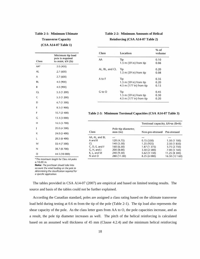
18

Table 2-2: Minimum Amounts of Helical

Reinforcing (CSA A14-07 Table 2)

Table 2-1: Minimum Ultimate

Transverse Capacity

(CSA A14-07 Table 1)

Table 2-3: Minimum Torsional Capacities (CSA A14-07 Table 3)

The tables provided in CSA A14-07 (2007) are empirical and based on limited testing results. The

source and basis of the tables could not be further explained.

According the Canadian standard, poles are assigned a class rating based on the ultimate transverse

load held during testing at 0.6 m from the tip of the pole (Table 2-1). The tip load also represents the

shear capacity of the pole. As the class letter goes from AA to O, the pole capacities increase, and as

a result, the pole tip diameter increases as well. The pitch of the helical reinforcing is calculated

based on an assumed wall thickness of 45 mm (Clause 4.2.4) and the minimum helical reinforcing

19

amounts found in Table 2-2. The minimum torsional capacities expected from poles reinforced with

the minimum helical reinforcing values are indicated in Table 2-3. CSA A14-07 (2007) states that

poles of class AA, AL, and BL should not be used in torsion applications and therefore no minimum

torsional capacities are listed Table 2-3 (Clause 4.2.6). Clause 4.2.5 recommends two methods for

the placement of the helical reinforcing: either all the required helical reinforcing is wound in one

direction or an overlapping system is used where half of the required reinforcing is wound in each

direction.

When needed, the Canadian code states that poles can be designed for torsional strengths in excess

of Table 2-3. It indicates that the pole designs should be based on empirical methods (Clause 4.3.4.2)

and that the poles should have helical reinforcement wound in both directions with a maximum pitch

of 1/5 of the pole diameter measured anywhere along the length (Clause 4.3.4.3).

In addition to the helical steel required for torsion, the minimum amount of helical reinforcing was

added originally to prevent splitting of the pole due to the transfer of prestressing forces and other

environmental effects (CSA A14-M1979, 1979). According to the CSA A14-M1979 (1979),

additional spiral reinforcement requirements were included to prevent splitting at the butt of the pole.

The standard also states that the splitting of the butt may be related to the cycles of freeze and thaw

and concrete poles manufacturers in Southern Ontario determined that including additional spiral

reinforcement to the reinforcement required for torsional strength solved the problem of splitting at

the butt of the pole (preface of CSA A14-M1979, 1979). Studies conducted by Dilger et al. (1996;

1997) and Wang et al. (2001), on the other hand, indicate that the addition of helical steel to prevent

splitting at the butt of the pole was incorrect. The addition of more steel to prevent splitting would

only cause further problems. With more helical steel in the pole, there would be more of a possibility

for corrosion and eventual spalling of the concrete. Special consideration to the concrete mixes and

elimination of concrete segregation would be better than the addition of helical steel.

The requirements added by the CSA A14-M1979 standard are stated in Clause 4.4, helical

reinforcement. Clause 4.4.1 states that helical reinforcement is included for torsional strength and to

reinforce areas of the pole that contain openings. A helical steel reinforcement ratio of 0.1 percent of

the concrete wall area was recommended (Clause 4.4.4). The old standard suggested using 3 mm

wire at pitches varying from 100 mm at the tip to 300 mm at the butt along the full length of the pole

to control cracking. The interior 13 mm of wall thickness was also neglected in the calculation of the

helical reinforcement amount for spun concrete poles according to the 1979 code. The reduction in

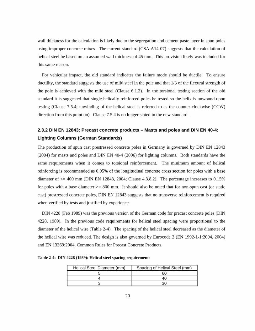
20

wall thickness for the calculation is likely due to the segregation and cement paste layer in spun poles

using improper concrete mixes. The current standard (CSA A14-07) suggests that the calculation of

helical steel be based on an assumed wall thickness of 45 mm. This provision likely was included for

this same reason.

For vehicular impact, the old standard indicates the failure mode should be ductile. To ensure

ductility, the standard suggests the use of mild steel in the pole and that 1/3 of the flexural strength of

the pole is achieved with the mild steel (Clause 6.1.3). In the torsional testing section of the old

standard it is suggested that single helically reinforced poles be tested so the helix is unwound upon

testing (Clause 7.5.4; unwinding of the helical steel is referred to as the counter clockwise (CCW)

direction from this point on). Clause 7.5.4 is no longer stated in the new standard.

2.3.2 DIN EN 12843: Precast concrete products – Masts and poles and DIN EN 40-4: Lighting Columns (German Standards)

The production of spun cast prestressed concrete poles in Germany is governed by DIN EN 12843

(2004) for masts and poles and DIN EN 40-4 (2006) for lighting columns. Both standards have the

same requirements when it comes to torsional reinforcement. The minimum amount of helical

reinforcing is recommended as 0.05% of the longitudinal concrete cross section for poles with a base

diameter of <= 400 mm (DIN EN 12843, 2004; Clause 4.3.8.2). The percentage increases to 0.15%

for poles with a base diameter >= 800 mm. It should also be noted that for non-spun cast (or static

cast) prestressed concrete poles, DIN EN 12843 suggests that no transverse reinforcement is required

when verified by tests and justified by experience.

DIN 4228 (Feb 1989) was the previous version of the German code for precast concrete poles (DIN

4228, 1989). In the previous code requirements for helical steel spacing were proportional to the

diameter of the helical wire (Table 2-4). The spacing of the helical steel decreased as the diameter of

the helical wire was reduced. The design is also governed by Eurocode 2 (EN 1992-1-1:2004, 2004)

and EN 13369:2004, Common Rules for Precast Concrete Products.

Table 2-4: DIN 4228 (1989): Helical steel spacing requirements

Helical Steel Diameter (mm) Spacing of Helical Steel (mm) 5 60 4 40 3 30

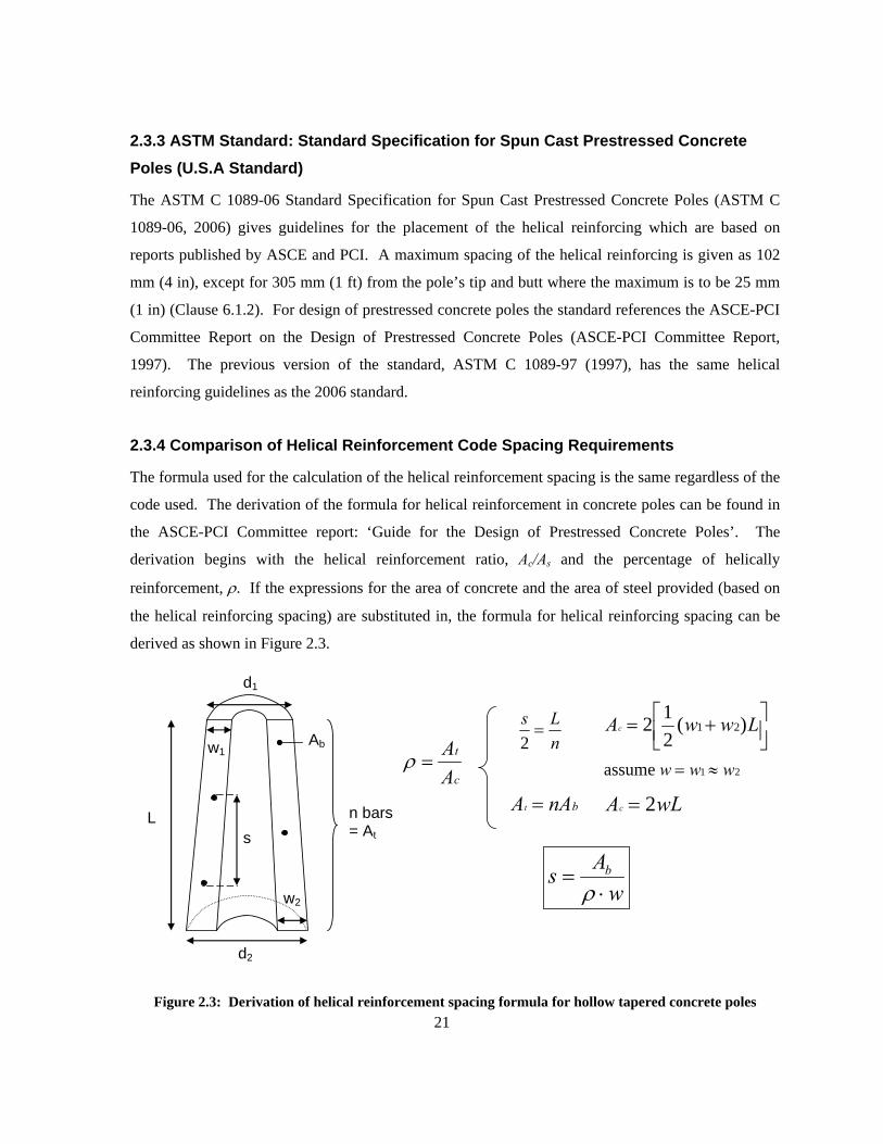
21

2.3.3 ASTM Standard: Standard Specification for Spun Cast Prestressed Concrete Poles (U.S.A Standard)

The ASTM C 1089-06 Standard Specification for Spun Cast Prestressed Concrete Poles (ASTM C

1089-06, 2006) gives guidelines for the placement of the helical reinforcing which are based on

reports published by ASCE and PCI. A maximum spacing of the helical reinforcing is given as 102

mm (4 in), except for 305 mm (1 ft) from the pole’s tip and butt where the maximum is to be 25 mm

(1 in) (Clause 6.1.2). For design of prestressed concrete poles the standard references the ASCE-PCI

Committee Report on the Design of Prestressed Concrete Poles (ASCE-PCI Committee Report,

1997). The previous version of the standard, ASTM C 1089-97 (1997), has the same helical

reinforcing guidelines as the 2006 standard.

2.3.4 Comparison of Helical Reinforcement Code Spacing Requirements

The formula used for the calculation of the helical reinforcement spacing is the same regardless of the

code used. The derivation of the formula for helical reinforcement in concrete poles can be found in

the ASCE-PCI Committee report: ‘Guide for the Design of Prestressed Concrete Poles’. The

derivation begins with the helical reinforcement ratio, Ac/As and the percentage of helically

reinforcement, ρ. If the expressions for the area of concrete and the area of steel provided (based on

the helical reinforcing spacing) are substituted in, the formula for helical reinforcing spacing can be

derived as shown in Figure 2.3.

L

d1

d2

w1

w2

Ab

n bars= Ats

⎥⎦⎤

⎢⎣⎡ += LwwAc )(212 21

wAs b

⋅=

ρ

c

t

AA

=ρ

bnAAt =

nLs

=2

21 assume www ≈=

wLAc 2=

Figure 2.3: Derivation of helical reinforcement spacing formula for hollow tapered concrete poles

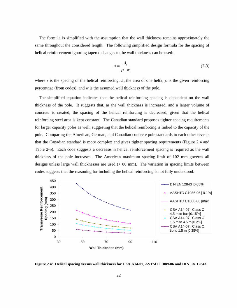
22

The formula is simplified with the assumption that the wall thickness remains approximately the

same throughout the considered length. The following simplified design formula for the spacing of

helical reinforcement ignoring tapered changes to the wall thickness can be used:

w

As s

⋅=

ρ (2-3)

where s is the spacing of the helical reinforcing, As the area of one helix, ρ is the given reinforcing

percentage (from codes), and w is the assumed wall thickness of the pole.

The simplified equation indicates that the helical reinforcing spacing is dependent on the wall

thickness of the pole. It suggests that, as the wall thickness is increased, and a larger volume of

concrete is created, the spacing of the helical reinforcing is decreased, given that the helical

reinforcing steel area is kept constant. The Canadian standard proposes tighter spacing requirements

for larger capacity poles as well, suggesting that the helical reinforcing is linked to the capacity of the

pole. Comparing the American, German, and Canadian concrete pole standards to each other reveals

that the Canadian standard is more complex and gives tighter spacing requirements (Figure 2.4 and

Table 2-5). Each code suggests a decrease in helical reinforcement spacing is required as the wall

thickness of the pole increases. The American maximum spacing limit of 102 mm governs all

designs unless large wall thicknesses are used (> 80 mm). The variation in spacing limits between

codes suggests that the reasoning for including the helical reinforcing is not fully understood.

0

50

100

150

200

250

300

350

400

450

30 50 70 90 110

Wall Thickness (mm)

Tran

sver

se R

einf

orce

men

t Sp

acin

g (m

m)

DIN EN 12843 [0.05%]

AASHTO C1086-06 [ 0.1%]

AASHTO C1086-06 [max]

CSA A14-07: Class C 4.5 m to butt [0.15%]CSA A14-07: Class C 1.5 m to 4.5 m [0.2%]CSA A14-07: Class C tip to 1.5 m [0.35%]

Figure 2.4: Helical spacing versus wall thickness for CSA A14-07, ASTM C 1089-06 and DIN EN 12843

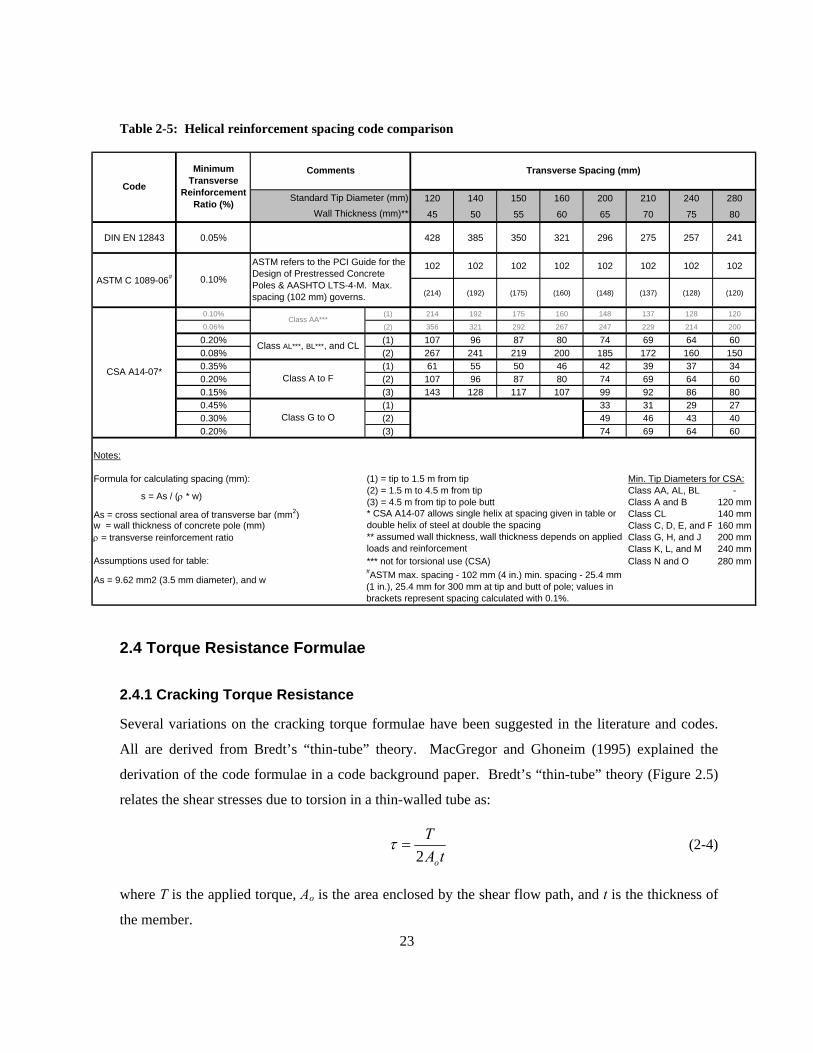
23

Table 2-5: Helical reinforcement spacing code comparison

120 140 150 160 200 210 240 280

45 50 55 60 65 70 75 80

DIN EN 12843 0.05% 428 385 350 321 296 275 257 241

102 102 102 102 102 102 102 102

(214) (192) (175) (160) (148) (137) (128) (120)

0.10% (1) 214 192 175 160 148 137 128 120

0.06% (2) 356 321 292 267 247 229 214 200

0.20% (1) 107 96 87 80 74 69 64 600.08% (2) 267 241 219 200 185 172 160 1500.35% (1) 61 55 50 46 42 39 37 340.20% (2) 107 96 87 80 74 69 64 600.15% (3) 143 128 117 107 99 92 86 800.45% (1) 33 31 29 270.30% (2) 49 46 43 400.20% (3) 74 69 64 60

Notes:

Formula for calculating spacing (mm): (1) = tip to 1.5 m from tip Min. Tip Diameters for CSA:(2) = 1.5 m to 4.5 m from tip Class AA, AL, BL -(3) = 4.5 m from tip to pole butt Class A and B 120 mm

As = cross sectional area of transverse bar (mm2) Class CL 140 mmw = wall thickness of concrete pole (mm) Class C, D, E, and F 160 mmρ = transverse reinforcement ratio Class G, H, and J 200 mm

Class K, L, and M 240 mm*** not for torsional use (CSA) Class N and O 280 mm

s = As / (ρ * w)

Standard Tip Diameter (mm)

Wall Thickness (mm)**

Minimum Transverse

Reinforcement Ratio (%)

Code

CSA A14-07*

Class AA***

ASTM refers to the PCI Guide for the Design of Prestressed Concrete Poles & AASHTO LTS-4-M. Max. spacing (102 mm) governs.

0.10%ASTM C 1089-06#

Comments Transverse Spacing (mm)

Class G to O

Class AL***, BL***, and CL

Class A to F

* CSA A14-07 allows single helix at spacing given in table or double helix of steel at double the spacing** assumed wall thickness, wall thickness depends on applied loads and reinforcement

As = 9.62 mm2 (3.5 mm diameter), and w

Assumptions used for table:#ASTM max. spacing - 102 mm (4 in.) min. spacing - 25.4 mm (1 in.), 25.4 mm for 300 mm at tip and butt of pole; values in brackets represent spacing calculated with 0.1%.

2.4 Torque Resistance Formulae

2.4.1 Cracking Torque Resistance

Several variations on the cracking torque formulae have been suggested in the literature and codes.

All are derived from Bredt’s “thin-tube” theory. MacGregor and Ghoneim (1995) explained the

derivation of the code formulae in a code background paper. Bredt’s “thin-tube” theory (Figure 2.5)

relates the shear stresses due to torsion in a thin-walled tube as:

tA

T

o2=τ (2-4)

where T is the applied torque, Ao is the area enclosed by the shear flow path, and t is the thickness of

the member.

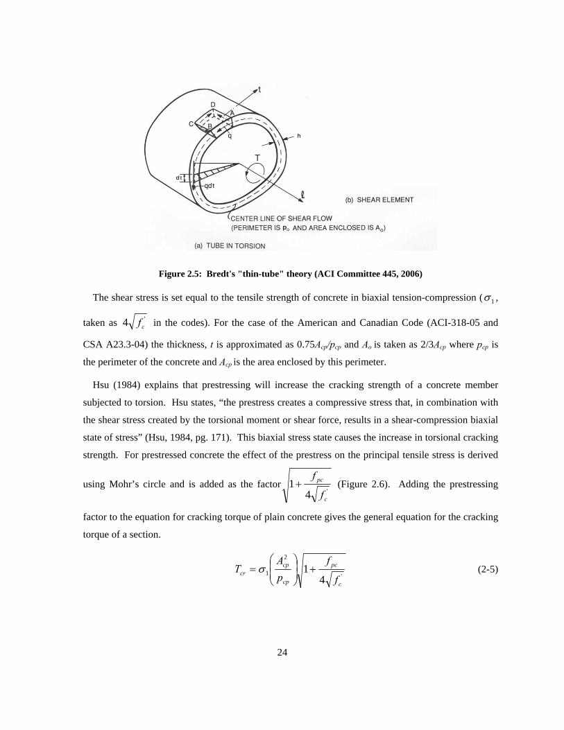
24

Figure 2.5: Bredt's "thin-tube" theory (ACI Committee 445, 2006)

The shear stress is set equal to the tensile strength of concrete in biaxial tension-compression ( 1σ ,

taken as '4 cf in the codes). For the case of the American and Canadian Code (ACI-318-05 and

CSA A23.3-04) the thickness, t is approximated as 0.75Acp/pcp and Ao is taken as 2/3Acp where pcp is

the perimeter of the concrete and Acp is the area enclosed by this perimeter.

Hsu (1984) explains that prestressing will increase the cracking strength of a concrete member

subjected to torsion. Hsu states, “the prestress creates a compressive stress that, in combination with

the shear stress created by the torsional moment or shear force, results in a shear-compression biaxial

state of stress” (Hsu, 1984, pg. 171). This biaxial stress state causes the increase in torsional cracking

strength. For prestressed concrete the effect of the prestress on the principal tensile stress is derived

using Mohr’s circle and is added as the factor'4

1c

pc

f

f+ (Figure 2.6). Adding the prestressing

factor to the equation for cracking torque of plain concrete gives the general equation for the cracking

torque of a section.

'

2

14

1c

pc

cp

cpcr

f

fpA

T +⎟⎟⎠

⎞⎜⎜⎝

⎛= σ (2-5)

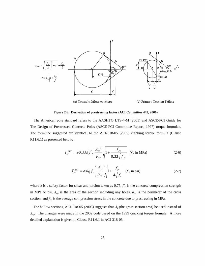
25

Figure 2.6: Derivation of prestressing factor (ACI Committee 445, 2006)

The American pole standard refers to the AASHTO LTS-4-M (2001) and ASCE-PCI Guide for

The Design of Prestressed Concrete Poles (ASCE-PCI Committee Report, 1997) torque formulae.

The formulae suggested are identical to the ACI-318-05 (2005) cracking torque formula (Clause

R11.6.1) as presented below:

c

pc

cp

cpc

ACIcr

f

fpA

fT'

2'

33.0133.0 += φ (f’c in MPa) (2-6)

'

2'

414

c

pc

cp

cpc

ACIcr

f

fpA

fT +⎟⎟⎠

⎞⎜⎜⎝

⎛= φ (f’c in psi) (2-7)

where φ is a safety factor for shear and torsion taken as 0.75, f`c is the concrete compression strength

in MPa or psi, Acp is the area of the section including any holes, pcp is the perimeter of the cross

section, and fcp is the average compression stress in the concrete due to prestressing in MPa.

For hollow sections, ACI-318-05 (2005) suggests that Ag (the gross section area) be used instead of

Acp. The changes were made in the 2002 code based on the 1999 cracking torque formula. A more

detailed explanation is given in Clause R11.6.1 in ACI-318-05.

26

The formula given in CSA A23.3-04 (2004) Canadian concrete standard is practically identical

except modified to work with the safety factors given in the Canadian code. In fact, the 0.38 factor is

derived from the 0.33 factor from ACI and multiplied by the 0.75 ACI safety factor and divided by

the 0.65 CSA concrete material safety factor.

cc

cppcc

c

cCSAcr

f

ff

pA

T'

'2

38.0138.0

λφ

φλφ +⎟

⎟⎠

⎞⎜⎜⎝

⎛= (f’c in MPa) (2-8)

where λ is a factor for low density concrete (taken as 1 for normal concrete), φc is a material safety

factor taken as 0.65 or 0.7 for precast concrete (Clause 16.1.3), f`c is the concrete compression

strength in MPa, Ac is the area of the section including any holes, pc is the perimeter of the cross

section, φp is a material safety factor for prestressing steel taken as 0.9, and fpc is the average

compression stress in the concrete due to prestressing in MPa. For hollow sections Ac is replaced by

1.5Ag if the wall thickness is less than 0.75Ac/pc.

The torsional formulae from the CHBDC (CAN/CSA-S6-06, 2006) are similar to those in the CSA

A23.3-04 (2004). Torsion is considered significant in the design of a member if the factored torsional

load is greater than a quarter of the cracking torque (CHBDC, Clause 8.9.1.1). The cracking torque

formula is identical to the formula from CSA A23.3-04 (2004) but uses a factor 0.32 (0.8 multiplied

by 0.4 from the fcr term) instead of 0.38 for the biaxial tension compression strength of concrete

(CHBDC, Clause 8.9.1.1).

crc

ce

cp

cpcrccr f

fpA

fTφ

φ80.0

180.02

+= (2-9)

where fcr = '4.0 cf for normal concrete, and fce is the stress in the concrete due to prestressing and

75.0=cφ .

In the German (DIN EN 12843) pole standard, Eurocode 2 (EC 2-1-1:2004, 2004) is referenced to

calculate the torsional capacities of poles. EC2 is identical to the German concrete standard, DIN

1045 (2001). Similar to the cracking torque formulae presented for ACI and CSA, EC2 suggests the

following formula (taken from Clause 6.3.2, and adding the prestressing effects included by Mohr’s

circle and the equation for the tensile strength of concrete):

27

ctd

cpctdiefk

ECcr f

ftATσ

+= 12 ,2 (2-10)

c

ctkctctd

ff

γα 05.0, where = , ctmctk ff 7.005.0, = ,

concrete MPa 50 for 10

1ln12.2

concrete MPa 50 for 30.0 )3/2(

>⎟⎠⎞

⎜⎝⎛ +

≤=

ckcm

ckck

ctm ffff

f

)(8 and MPaff ckcm += . Ak is the area enclosed by the centerline of the shear flow thickness

including hollow area, tef,i is the effective wall thickness taken as A/u but not less than twice the

distance between the edge and centre of the longitudinal reinforcement (hollow sections use real

thickness as an upper limit), A is the total area of the cross section including hollow areas, u is the

circumference of the cross section, σcp is the compressive stress in the concrete due to prestressing,

and fctd is the design tensile strength of the concrete. αct is a factor for long term effects normally

taken as 1, γc is the partial safety factor for concrete (1.5 for persistent or transient loads, 1.2 for

accidental or 1.0 for unfactored), and fctk,0.05 is the 5% fractal of the characteristic tensile strength of

concrete. The mean characteristic tensile strength is represented as fctm and the characteristic concrete

compressive strength (equivalent to 'cf ) is fck. fcm is the mean characteristic compressive strength.

The formulae used in the ASCE-PCI Guide (ASCE-PCI Committee Report, 1997) and AASHTO

LTS-4-M (2001) are the same as the formulae given in the ACI-318-05 (2005). The previous

AASHTO LTS-3 (1994) standard recommended the use of equations modified from the American

Concrete Institute standard at that time for nominal moment strength provided by concrete (discussed

in AASHTO 1994 – 1986 Commentary). It included an axial stress factor, FN. Axial stresses, due to

prestressing, increase the torsional capacity. An upper limit of 2 for FN was assumed as a reasonable

limit due to the limited research data available for the torsional capacity of prestressed concrete

without stirrups. For ultimate strength design torsional strengths are given by the following equation

for hollow poles with a inner diameter not more than one-half the pole diameter or width:

SVNpcAASHTO

u FFFdfT 394, 066.0 ′= (2-11)

where cf ′ in MPa

FN = axial stress factor = (1 + 0.29FP / Ac) where Ac is area of concrete in m2

FP = total prestress force after losses in MN

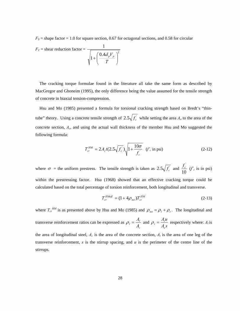
28

FS = shape factor = 1.0 for square section, 0.67 for octagonal sections, and 0.58 for circular

FV = shear reduction factor = 24.0

1

1

⎟⎟⎠

⎞⎜⎜⎝

⎛+

TVd pp

The cracking torque formulae found in the literature all take the same form as described by

MacGregor and Ghoneim (1995), the only difference being the value assumed for the tensile strength

of concrete in biaxial tension-compression.

Hsu and Mo (1985) presented a formula for torsional cracking strength based on Bredt’s “thin-

tube” theory. Using a concrete tensile strength of '5.2 cf while setting the area Ao to the area of the

concrete section, Ac, and using the actual wall thickness of the member Hsu and Mo suggested the

following formula:

`` 101)5.2(2

ccc

HMcr f

ftAT σ+= (f’c in psi) (2-12)

where σ = the uniform prestress. The tensile strength is taken as '5.2 cf and 10

`cf (f`c is in psi)

within the prestressing factor. Hsu (1968) showed that an effective cracking torque could be

calculated based on the total percentage of torsion reinforcement, both longitudinal and transverse.

HMcrtot

HMeffcr TT )41( ρ+= (2-13)

where TcrHM is as presented above by Hsu and Mo (1985) and tltot ρρρ += . The longitudinal and

transverse reinforcement ratios can be expressed as c

ll A

A=ρ and

sAuA

c

tt =ρ respectively where: Al is

the area of longitudinal steel, Ac is the area of the concrete section, At is the area of one leg of the

transverse reinforcement, s is the stirrup spacing, and u is the perimeter of the centre line of the

stirrups.

29

Rahal and Collins (1996) suggested a formula similar to the CSA equation (CSA A23.3-04, 2004),

but used '5 cf instead for the tensile strength of the concrete. The resulting equation for cracking

torque is:

'

2'

515

c

pc

c

cc

RCcr

f

fpA

fT +⎟⎟⎠

⎞⎜⎜⎝

⎛= (f’c in psi) (2-14)

Similar to Rahal and Collins, Ghoneim and MacGregor (1993) suggested the following formula for

cracking torque:

'

2'

46.0146.0

c

pc

c

cc

GMcr

f

fpA

fT +⎟⎟⎠

⎞⎜⎜⎝

⎛= (f’c in MPa) (2-15)

It should be noted that the Tcr equation suggested by Ghoneim and MacGregor (1993) and Rahal

and Collins (1996) are for beams subjected to pure torsion whereas the formulae provided by the

codes are for combined stresses (Koutchoukai and Belarbi, 2001). The result is that the equations

presented by all authors are 40% larger than the code values (Koutchoukai and Belarbi, 2001).

2.4.2 Ultimate Torsional Resistance

The ‘State of the Art Report: Design for Torsion in Concrete Structures’ by ACI Committee 445

(2006) presents the development of Rausch’s space truss model for torsion which is the basis for all

codes equations (ACI, CSA, EC2). Presented in the three paragraphs below is a summary of the

development from the ACI Committee report.

Ritter (1899) and Mörsch (1902) developed the first theories for shear using a plane truss model

consisting of struts and ties. The reinforced concrete member was constructed using compressive

carrying struts (concrete) and tension carrying ties (steel). The concept of the struts and ties gave a

simple approach to solving shear problems. Rausch extended the 2-D plane truss model developed by

Ritter and Mörsch and added the lever arm area idea proposed by Bredt in his “thin-tube” theory.

The space truss model developed by Rausch, in 1927 gave the first theory for torsion. Rausch’s

space truss model resisted the applied torsional moment by diagonal concrete compressive struts and

steel tension ties in the longitudinal and transverse direction (Figure 2.7). Rausch also assumed that

the struts were at an angle of 45 degrees and the ties were connected by hinges at the joints. The

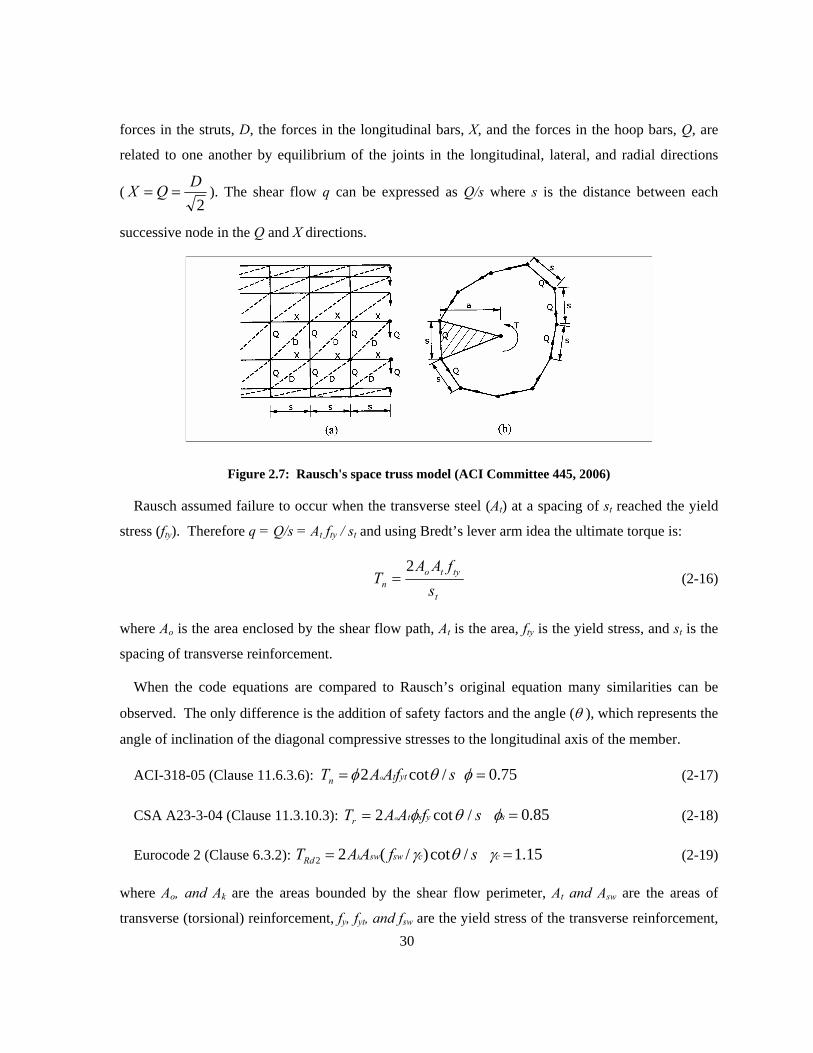
30

forces in the struts, D, the forces in the longitudinal bars, X, and the forces in the hoop bars, Q, are

related to one another by equilibrium of the joints in the longitudinal, lateral, and radial directions

(2

DQX == ). The shear flow q can be expressed as Q/s where s is the distance between each

successive node in the Q and X directions.

Figure 2.7: Rausch's space truss model (ACI Committee 445, 2006)

Rausch assumed failure to occur when the transverse steel (At) at a spacing of st reached the yield

stress (fty). Therefore q = Q/s = At fty / st and using Bredt’s lever arm idea the ultimate torque is:

t

tyton s

fAAT

2= (2-16)

where Ao is the area enclosed by the shear flow path, At is the area, fty is the yield stress, and st is the

spacing of transverse reinforcement.

When the code equations are compared to Rausch’s original equation many similarities can be

observed. The only difference is the addition of safety factors and the angle (θ ), which represents the

angle of inclination of the diagonal compressive stresses to the longitudinal axis of the member.

ACI-318-05 (Clause 11.6.3.6): sfAAT yttn o /cot2 θφ= 75.0=φ (2-17)

CSA A23-3-04 (Clause 11.3.10.3): sfAAT ystr o /cot2 θφ= 85.0=sφ (2-18)

Eurocode 2 (Clause 6.3.2): sfAAT cswswRd k /cot)/(22 θγ= 15.1=cγ (2-19)

where Ao, and Ak are the areas bounded by the shear flow perimeter, At and Asw are the areas of

transverse (torsional) reinforcement, fy, fyt, and fsw are the yield stress of the transverse reinforcement,

31

and s is the spacing of the transverse reinforcement. θ is the angle of inclination of the diagonal

compressive stresses and φ, φs, and γc are the code specific safety factors.

The CHBDC and CSA A23.3-04 provide the same formula for calculating the ultimate torsional

resistance of a section, except a higher material resistance is used for the prestressing and reinforcing

steel (0.95 and 0.90 respectively).

In addition each code has additional clauses for checking the adequate amount of longitudinal

reinforcing and cross section/concrete strut crushing strengths. The lowest value is taken then as the

ultimate torsional resistance. In the case of concrete poles the cross section is usually strong enough

for crushing and the governing factor is the transverse/helical reinforcement.

2.5 Minimum Transverse Reinforcing Spacing

Transverse reinforcement for torsion in all codes is determined by setting Tr > Tf and adding the

amount to the transverse reinforcement required for shear. Tr is calculated using the formulae given

in section 2.4.2. In the case of CSA A23.3-04 (2004) and ACI-318-05 (2005), if Tf is less than

0.25Tcr then torsional transverse reinforcement is not required.

The minimum transverse reinforcement requirements for torsion are based on the minimum shear

reinforcing requirements and are empirically based. ACI gives the following minimum requirement

for shear and torsion transverse reinforcement (Clause 11.6.5.4):

⎟⎟⎠

⎞⎜⎜⎝

⎛=+

yt

wc

tv f

sbfAA '75.02

(Imperial units) but not less than (50bws)/fyt (2-20)

⎟⎟⎠

⎞⎜⎜⎝

⎛=+

yt

wc

tv f

sbfAA '0625.02

(SI units: 0.0625 = 1/16) but not less than (0.33bws)/fyt (2-21)

where Av is the area of shear reinforcement (in2, mm2), At is the area of torsional reinforcement (in2,

mm2), f`c is the concrete compressive strength (psi, MPa), bw is the width of the web (in, mm), s is the

spacing of the transverse reinforcement (in, mm), and fyt is the yield stress of the transverse

reinforcement (psi, MPa).

Clause 11.5.6.3 indicates that the minimum shear reinforcement, Av,min is equal to the right hand

side of the equations above. For prestressed members it is suggested that the minimum shear

reinforcement be the smaller of Clause 11.5.6.3 and 11.5.6.4 (shown below):

32

wyd

pupsv b

df

sfAA

80min, = (Imperial units) (2-22)

where Av,min is the minimum area of shear reinforcement (in2), Aps is the area of prestressing

reinforcement (in2), fpu is the prestressing ultimate stress (psi), bw is the width of the web (in), s is the

spacing of the transverse reinforcement (in), d is the distance from the compressive flange to the

reinforcing steel (in), and fyd is the yield stress of the transverse reinforcement (psi).

The maximum spacing for transverse reinforcement according to ACI-318-05 is as follows (Clause

11.5.5.1):

d/2 for non-prestressed members

0.75h for prestressed members or 24 inches whichever smaller

where d is the distance from the compressive flange to the reinforcing steel, and h is the height of the

section.

ACI-318-05 Clause 11.5.5.2 gives another spacing requirement that at least one transverse

reinforcement steel bar must intercept a 45 degree inclined line to the member axis drawn through the

midpoint of the member extending to the flexural tension steel. In addition if the shear force in the

steel exceeds dbf wc'4 ( dbf wc

'33.0 ) then the requirements of Clause 11.5.5.1 and 11.5.5.2 must

be decreased by half (Clause 11.5.5.3). Clause 11.6.6 also limits the maximum spacing for transverse

torsional reinforcement as ph/8 (where ph is the perimeter at the level of the transverse reinforcement)

or 12 inches whichever smaller.

CSA A23.3-04 presents similar requirements to those of ACI-318-05 for minimum shear

reinforcement and maximum spacing. According to CSA Clause 11.3.8.1 torsional reinforcement can

be placed using spirals and the maximum spiral spacing is governed as follows:

If )125.0( 'pvwccf VdbfV +< φ or crf TT 25.0≤ then

smax is 600 mm or 0.7dv (where dv is the effective depth).

If )10.0( 'pvwccf VdbfV +> φ or crf TT 25.0> then Clause 11.3.8.3 reduces the requirements by

half to:


33

where f’c is the compressive strength in MPa, bw is the effective web width (mm), dv is the effective

shear depth (mm), Vp is the shear force due to prestressing (kN), Tf is the factored torsional moment,

Tcr is the cracking torque and smax is the maximum spacing of the transverse reinforcement (mm).

CSA A23.3-04 Clause 11.3.8.2 indicates one line of effective shear reinforcement must intercept a

line drawn at 35 degrees from the member axis. The minimum amount of transverse reinforcement is

given by Clause 11.2.8.2 and is calculated as follows:

⎟⎟⎠

⎞⎜⎜⎝

⎛=

y

wcv f

sbfA 'min, 06.0 (2-23)

where bw is the effective web width (mm) with the effective depth of the section (dv) (mm), s is the

spacing the reinforcing (mm), and fy is the reinforcement yield stress (MPa). For a solid circular

section bw is taken as the diameter (Clause 11.2.10.3).

The requirements are also very similar to those given in the CHBDC (CAN/CSA-S6-06, 2006).

According to CHBDC Clause 8.1.4.5.2 torsional reinforcement can be placed using spirals and the

maximum spiral spacing is governed as follows:

If )10.0( 'pvwccf VdbfV +< φ or crf TT 25.0≤ then


If )10.0( 'pvwccf VdbfV +> φ or crf TT 25.0> then


The minimum amount of transverse reinforcement is given by CHBDC Clause 8.9.1.3 and is

calculated using:

⎟⎟⎠

⎞⎜⎜⎝

⎛=

y

wcrv f

sbfA 15.0min, (2-24)

where bw is the effective web width with the effective depth of the section (dv), s is the spacing the

reinforcing, and fy is the reinforcement yield stress. For a solid circular section bw is taken as the

diameter. If the 0.4 factor is included from the fcr variable the formula given by Clause 8.9.1.3 gives

the 0.06 coefficient used in CSA A23-3-04 (2004).

EC-2 suggests the minimum shear reinforcement be taken as (Clause 9.2.2 (5) and (6)):

34

⎟⎟⎠

⎞⎜⎜⎝

⎛=

yk

wckv f

sbfA 08.0min, (2-25)

where fck is the characteristic compressive strength (MPa), bw is the effective web width (mm), s is the

spacing of the transverse reinforcement (mm), and fyk is the characteristic yield stress of the transverse

reinforcement (MPa).

Maximum spacing of the transverse reinforcement, st,max is taken as 0.75d or 600 mm whichever is

less. For torsion Clause 9.2.3 (2) indicates that the minimum requirements for shear are generally

sufficient for minimum torsional reinforcement required.

The minimum requirements for torsion could alternatively be derived by setting Tr >= λTcr (Ali and

White, 1999 and Koutchoukali and Belarbi, 2001). The cracking torque is multiplied by a factor,

taken as 1.2 (Koutchoukali and Belarbi, 2001) or 1.5-1.7 (Ali and White, 1999), to include reserve

strength after cracking. Koutchoukali and Belarbi presented the following equation for the transverse

reinforcement requirements derived using the cracking torque equation given by Ghoneim and

MacGregor (1993):

coyt

cct

pAfAf

sA 2'

min

28.0=⎟⎠⎞

⎜⎝⎛ (2-26)

where At is the transverse reinforcement area (mm2), s is the spacing (mm), f’c is the compressive

stress in the concrete (MPa), Ac is the area of the concrete (mm2), fyt is the yield stress of the

transverse reinforcement (MPa), AO is the area enclosed by the shear flow path (mm2), and pc is the

perimeter of the concrete section (mm).

Similarly Ali and White (1999) derived an equation for minimum transverse reinforcement from

the ACI cracking torque formula relating to the longitudinal reinforcement and not the concrete

strength.

)(cot 2min θ

yl

yvh

lt

ff

p

AsA

=⎟⎠⎞

⎜⎝⎛ (2-27)

where At is the transverse reinforcement area (mm2), s is the spacing (mm), Al is the area of the

longitudinal reinforcement (mm2), fyv is the yield stress of the transverse reinforcement (MPa), fyl is

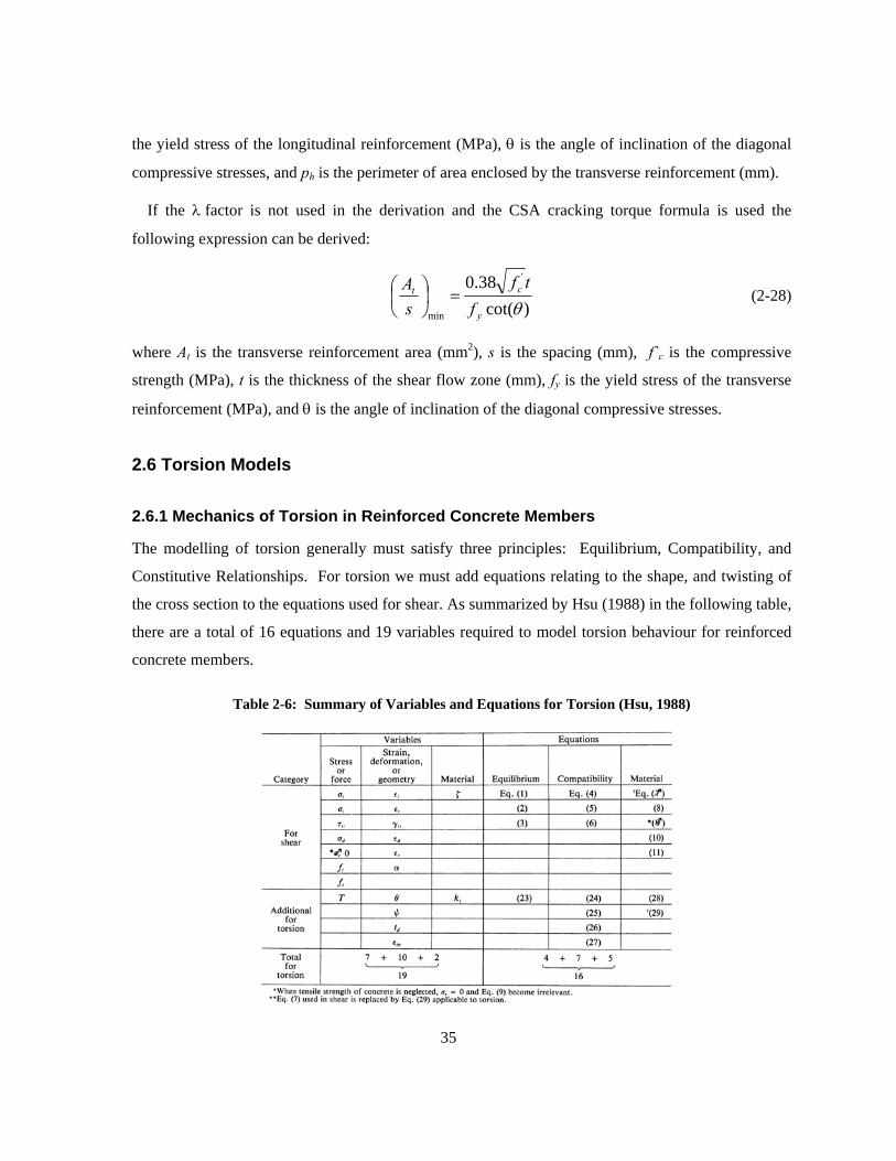
35

the yield stress of the longitudinal reinforcement (MPa), θ is the angle of inclination of the diagonal

compressive stresses, and ph is the perimeter of area enclosed by the transverse reinforcement (mm).

If the λ factor is not used in the derivation and the CSA cracking torque formula is used the

following expression can be derived:

)cot(

38.0 '

min θy

ct

ftf

sA

=⎟⎠⎞

⎜⎝⎛ (2-28)

where At is the transverse reinforcement area (mm2), s is the spacing (mm), f`c is the compressive

strength (MPa), t is the thickness of the shear flow zone (mm), fy is the yield stress of the transverse

reinforcement (MPa), and θ is the angle of inclination of the diagonal compressive stresses.

2.6 Torsion Models

2.6.1 Mechanics of Torsion in Reinforced Concrete Members

The modelling of torsion generally must satisfy three principles: Equilibrium, Compatibility, and

Constitutive Relationships. For torsion we must add equations relating to the shape, and twisting of

the cross section to the equations used for shear. As summarized by Hsu (1988) in the following table,

there are a total of 16 equations and 19 variables required to model torsion behaviour for reinforced

concrete members.

Table 2-6: Summary of Variables and Equations for Torsion (Hsu, 1988)

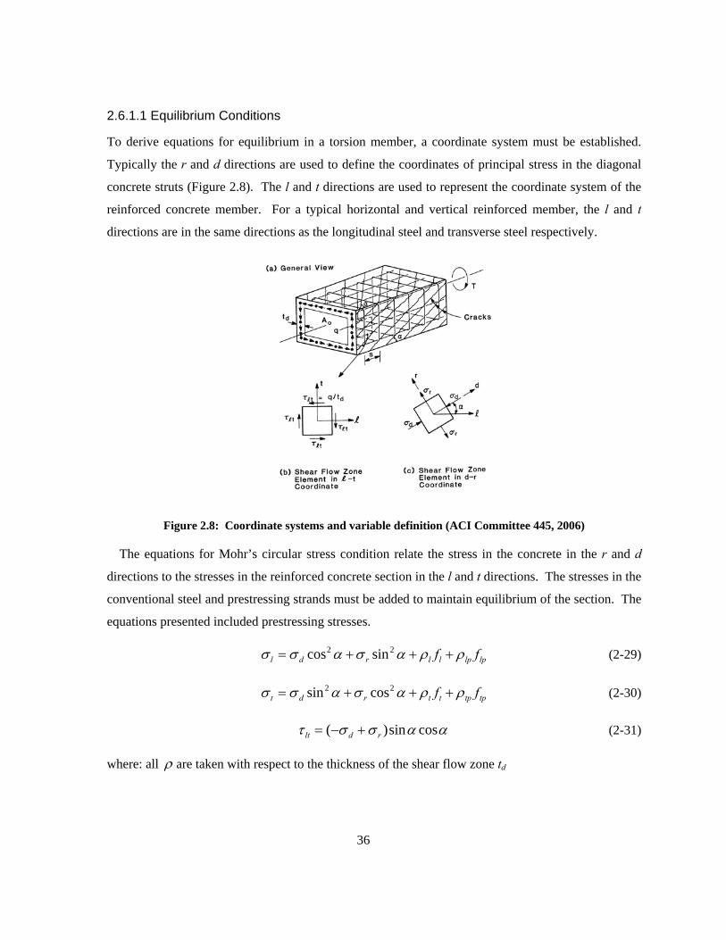
36

2.6.1.1 Equilibrium Conditions

To derive equations for equilibrium in a torsion member, a coordinate system must be established.

Typically the r and d directions are used to define the coordinates of principal stress in the diagonal

concrete struts (Figure 2.8). The l and t directions are used to represent the coordinate system of the

reinforced concrete member. For a typical horizontal and vertical reinforced member, the l and t

directions are in the same directions as the longitudinal steel and transverse steel respectively.

Figure 2.8: Coordinate systems and variable definition (ACI Committee 445, 2006)

The equations for Mohr’s circular stress condition relate the stress in the concrete in the r and d

directions to the stresses in the reinforced concrete section in the l and t directions. The stresses in the

conventional steel and prestressing strands must be added to maintain equilibrium of the section. The

equations presented included prestressing stresses.

lplpllrdl ff ρρασασσ +++= 22 sincos (2-29)

tptpttrdt ff ρρασασσ +++= 22 cossin (2-30)

αασστ cossin)( rdlt +−= (2-31)

where: all ρ are taken with respect to the thickness of the shear flow zone td

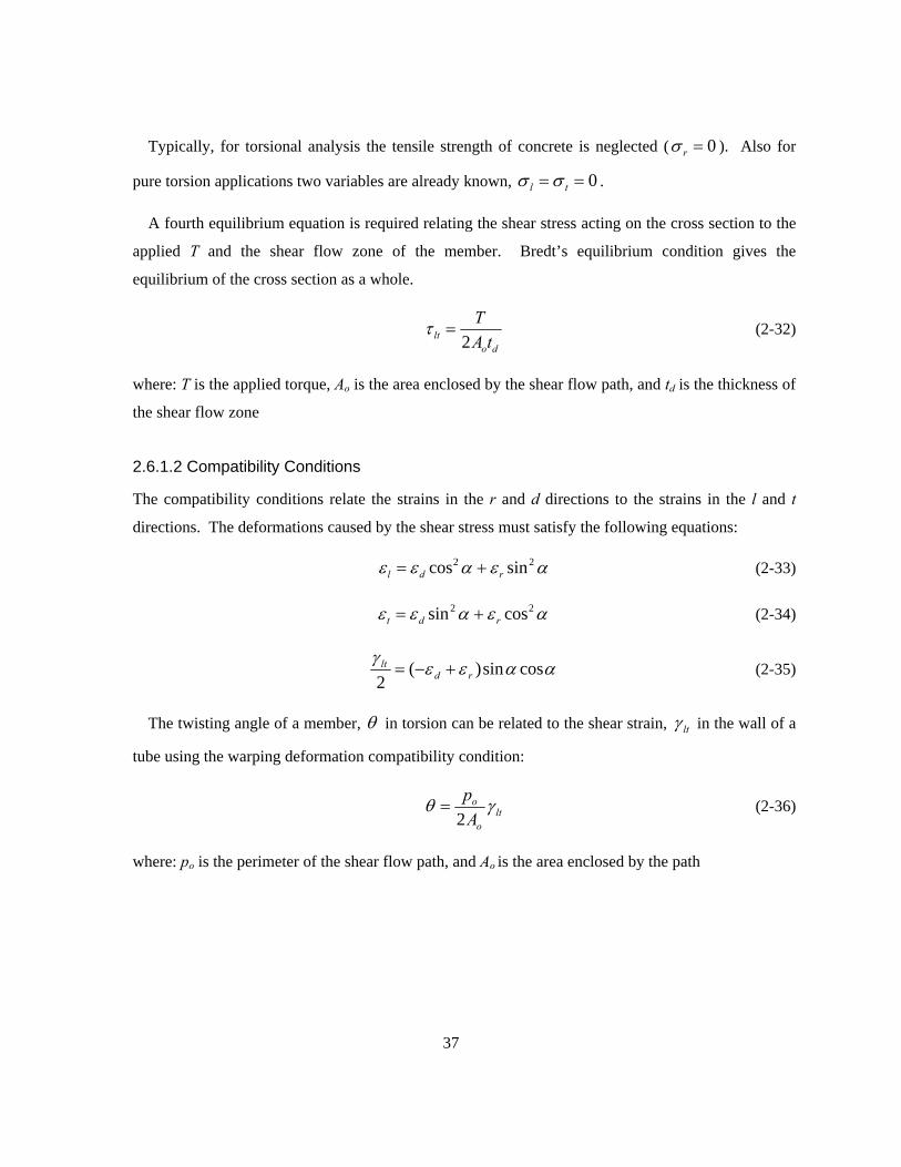
37

Typically, for torsional analysis the tensile strength of concrete is neglected ( 0=rσ ). Also for

pure torsion applications two variables are already known, 0== tl σσ .

A fourth equilibrium equation is required relating the shear stress acting on the cross section to the

applied T and the shear flow zone of the member. Bredt’s equilibrium condition gives the

equilibrium of the cross section as a whole.

do

lt tAT

2=τ (2-32)

where: T is the applied torque, Ao is the area enclosed by the shear flow path, and td is the thickness of

the shear flow zone

2.6.1.2 Compatibility Conditions

The compatibility conditions relate the strains in the r and d directions to the strains in the l and t

directions. The deformations caused by the shear stress must satisfy the following equations:

αεαεε 22 sincos rdl += (2-33)

αεαεε 22 cossin rdt += (2-34)

ααεεγ cossin)(2 rdlt +−= (2-35)

The twisting angle of a member, θ in torsion can be related to the shear strain, ltγ in the wall of a

tube using the warping deformation compatibility condition:

lto

o

Ap γθ

2= (2-36)

where: po is the perimeter of the shear flow path, and Ao is the area enclosed by the path

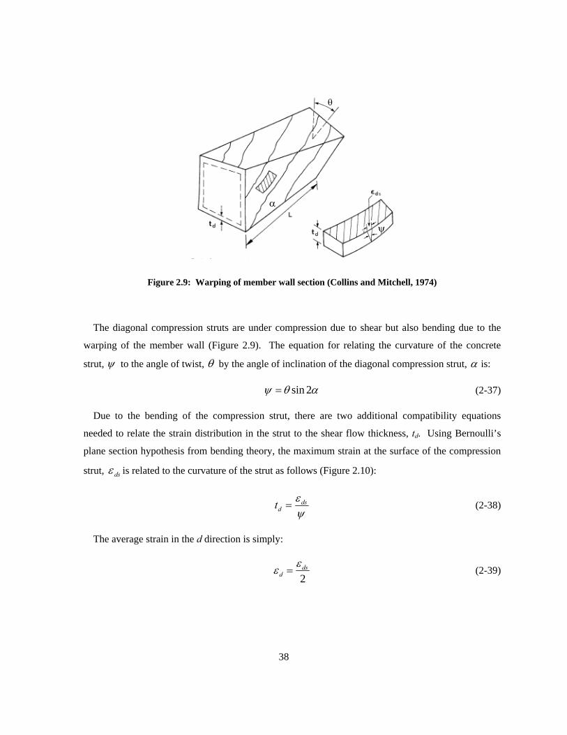
38

Figure 2.9: Warping of member wall section (Collins and Mitchell, 1974)

The diagonal compression struts are under compression due to shear but also bending due to the

warping of the member wall (Figure 2.9). The equation for relating the curvature of the concrete

strut, ψ to the angle of twist, θ by the angle of inclination of the diagonal compression strut, α is:

αθψ 2sin= (2-37)

Due to the bending of the compression strut, there are two additional compatibility equations

needed to relate the strain distribution in the strut to the shear flow thickness, td. Using Bernoulli’s

plane section hypothesis from bending theory, the maximum strain at the surface of the compression

strut, dsε is related to the curvature of the strut as follows (Figure 2.10):

ψε ds

dt = (2-38)

The average strain in the d direction is simply:

2ds

dεε = (2-39)

θ

ψ

α

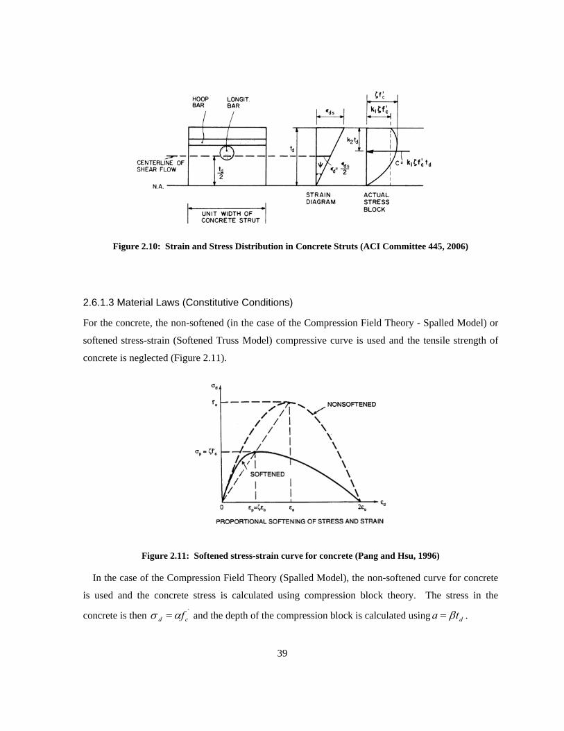
39

Figure 2.10: Strain and Stress Distribution in Concrete Struts (ACI Committee 445, 2006)

2.6.1.3 Material Laws (Constitutive Conditions)

For the concrete, the non-softened (in the case of the Compression Field Theory - Spalled Model) or

softened stress-strain (Softened Truss Model) compressive curve is used and the tensile strength of

concrete is neglected (Figure 2.11).

Figure 2.11: Softened stress-strain curve for concrete (Pang and Hsu, 1996)

In the case of the Compression Field Theory (Spalled Model), the non-softened curve for concrete

is used and the concrete stress is calculated using compression block theory. The stress in the

concrete is then `cd fασ = and the depth of the compression block is calculated using dta β= .

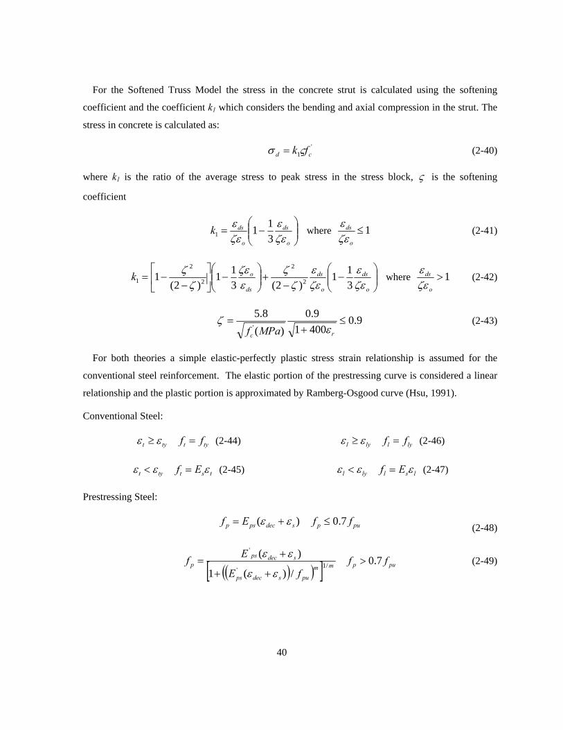
40

For the Softened Truss Model the stress in the concrete strut is calculated using the softening

coefficient and the coefficient k1 which considers the bending and axial compression in the strut. The

stress in concrete is calculated as:

'1 cd fk ςσ = (2-40)

where k1 is the ratio of the average stress to peak stress in the stress block, ς is the softening

coefficient

⎟⎟⎠

⎞⎜⎜⎝

⎛−=

o

ds

o

dskζεε

ζεε

3111 where 1≤

o

ds

ζεε

(2-41)

⎟⎟⎠

⎞⎜⎜⎝

⎛−

−+⎟⎟

⎠

⎞⎜⎜⎝

⎛−⎥

⎦

⎤⎢⎣

⎡−

−=o

ds

o

ds

ds

okζεε

ζεε

ζζ

εζε

ζζ

311

)2(311

)2(1 2

2

2

2

1 where 1>o

ds

ζεε

(2-42)

9.040019.0

)(8.5

'≤

+=

rc MPaf εζ (2-43)

For both theories a simple elastic-perfectly plastic stress strain relationship is assumed for the

conventional steel reinforcement. The elastic portion of the prestressing curve is considered a linear

relationship and the plastic portion is approximated by Ramberg-Osgood curve (Hsu, 1991).

Conventional Steel:

tyt εε ≥ tyt ff = (2-44)

tyt εε < tst Ef ε= (2-45)

lyl εε ≥ lyl ff = (2-46)

lyl εε < lsl Ef ε= (2-47)

Prestressing Steel:

)( sdecpsp Ef εε += pup ff 7.0≤ (2-48)

( )( )[ ] mm

pusdecps

sdecpsp

fE

Ef /1'

'

/)(1

)(⋅

++

+=

εε

εε pup ff 7.0> (2-49)

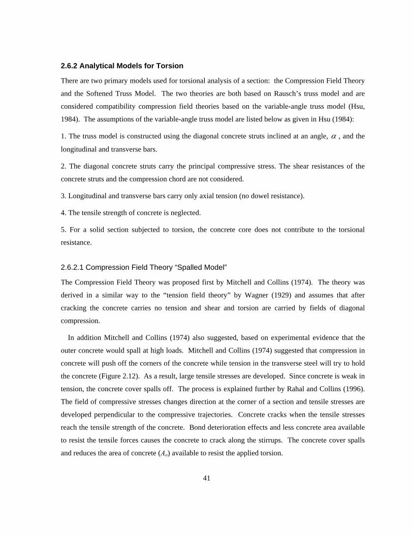
41

2.6.2 Analytical Models for Torsion

There are two primary models used for torsional analysis of a section: the Compression Field Theory

and the Softened Truss Model. The two theories are both based on Rausch’s truss model and are

considered compatibility compression field theories based on the variable-angle truss model (Hsu,

1984). The assumptions of the variable-angle truss model are listed below as given in Hsu (1984):

1. The truss model is constructed using the diagonal concrete struts inclined at an angle, α , and the

longitudinal and transverse bars.

2. The diagonal concrete struts carry the principal compressive stress. The shear resistances of the

concrete struts and the compression chord are not considered.

3. Longitudinal and transverse bars carry only axial tension (no dowel resistance).

4. The tensile strength of concrete is neglected.

5. For a solid section subjected to torsion, the concrete core does not contribute to the torsional

resistance.

2.6.2.1 Compression Field Theory “Spalled Model”

The Compression Field Theory was proposed first by Mitchell and Collins (1974). The theory was

derived in a similar way to the “tension field theory” by Wagner (1929) and assumes that after

cracking the concrete carries no tension and shear and torsion are carried by fields of diagonal

compression.

In addition Mitchell and Collins (1974) also suggested, based on experimental evidence that the

outer concrete would spall at high loads. Mitchell and Collins (1974) suggested that compression in

concrete will push off the corners of the concrete while tension in the transverse steel will try to hold

the concrete (Figure 2.12). As a result, large tensile stresses are developed. Since concrete is weak in

tension, the concrete cover spalls off. The process is explained further by Rahal and Collins (1996).

The field of compressive stresses changes direction at the corner of a section and tensile stresses are

developed perpendicular to the compressive trajectories. Concrete cracks when the tensile stresses

reach the tensile strength of the concrete. Bond deterioration effects and less concrete area available

to resist the tensile forces causes the concrete to crack along the stirrups. The concrete cover spalls

and reduces the area of concrete (Ao) available to resist the applied torsion.

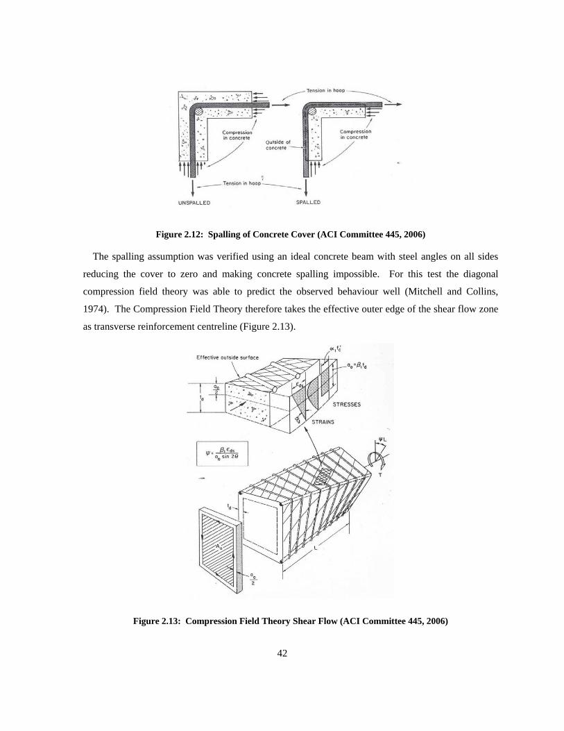
42

Figure 2.12: Spalling of Concrete Cover (ACI Committee 445, 2006)

The spalling assumption was verified using an ideal concrete beam with steel angles on all sides

reducing the cover to zero and making concrete spalling impossible. For this test the diagonal

compression field theory was able to predict the observed behaviour well (Mitchell and Collins,

1974). The Compression Field Theory therefore takes the effective outer edge of the shear flow zone

as transverse reinforcement centreline (Figure 2.13).

Figure 2.13: Compression Field Theory Shear Flow (ACI Committee 445, 2006)

43

The area enclosed by the shear flow path and perimeter of the shear flow path are taken as follows:

ho

oho paAA2

−= (2-50)

oho app 4−= (2-51)

where ao = β1td (stress block factors), Aoh is the area measured to the middle of the outer closed

stirrups, and ph is the outer perimeter of the cross section.

A typical solution for a pure torsion case would take the following form (from ACI Committee

445, 2006):

1. A value of strain is selected in the d direction.

2. The value of the equivalent depth of compression is then estimated.

3. Using the estimated depth of compression and the geometry the values Ao and po can be

calculated.

4. Tensile stresses in the longitudinal and transverse steel as well as the diagonal compressive

stresses can then be calculated from the truss equilibrium equations.

5. Strains in the l, t and d directions can be calculated and the values can be used to check the

estimated value of the compression depth.

6. Convergence the compression depth gives the torque resistance and twist of the member.

The full torque-twist curve is found by selecting varying values of strain in the d direction up to

0.0035.

2.6.2.2 Softened Truss Model

The Softened Truss Model was proposed by Hsu (1988) and is similar to the theory developed by

Collins and Mitchell. The Softened Truss Model used the same equilibrium and compatibility

equations but included the softening effects of the compressive strength of concrete. The Softened

Truss Model assumes that the concrete outside of the transverse reinforcement participates in resisting

the applied torsion and therefore no spalling of the concrete occurs (Figure 2.14).

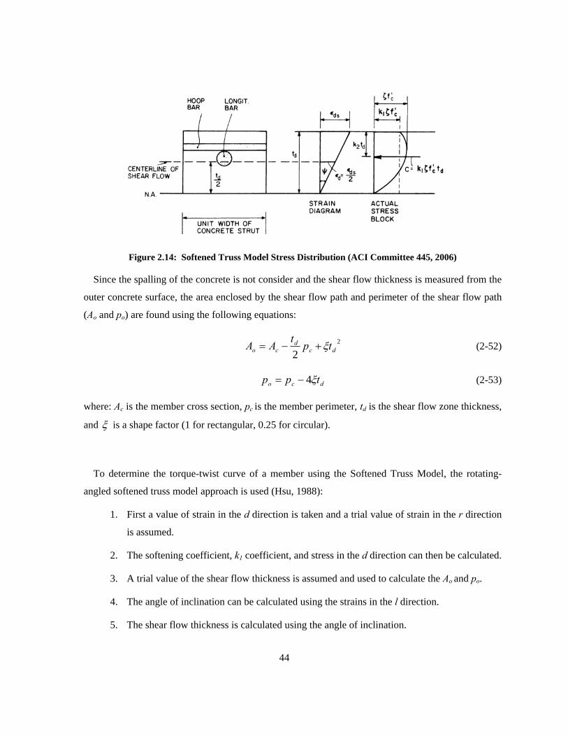
44

Figure 2.14: Softened Truss Model Stress Distribution (ACI Committee 445, 2006)

Since the spalling of the concrete is not consider and the shear flow thickness is measured from the

outer concrete surface, the area enclosed by the shear flow path and perimeter of the shear flow path

(Ao and po) are found using the following equations:

2

2 dcd

co tptAA ξ+−= (2-52)

dco tpp ξ4−= (2-53)

where: Ac is the member cross section, pc is the member perimeter, td is the shear flow zone thickness,

and ξ is a shape factor (1 for rectangular, 0.25 for circular).

To determine the torque-twist curve of a member using the Softened Truss Model, the rotating-

angled softened truss model approach is used (Hsu, 1988):

1. First a value of strain in the d direction is taken and a trial value of strain in the r direction

is assumed.

2. The softening coefficient, k1 coefficient, and stress in the d direction can then be calculated.

3. A trial value of the shear flow thickness is assumed and used to calculate the Ao and po.

4. The angle of inclination can be calculated using the strains in the l direction.

5. The shear flow thickness is calculated using the angle of inclination.

45

6. The strain in the r direction is calculated and yielding in the t direction is checked. If the

strain in r does not match the initial guess, a new value of strain in r is selected until

convergence occurs.

7. Once the strain has converged, the torque and twist values can be calculated.

The full torque-twist curve is found by selecting varying values of strain in the d direction up to

0.0035.

Another approach taken by Hsu and Zhang (1997) is the Fixed-Angled Softened Truss Model.

Instead of calculating the angle of inclination, it is a known variable and calculated from the applied

stresses in the l and t directions and the shear stress in the lt directions. Hsu and Zhang (1997) were

able to consistently achieve very good results with the Fixed-Angled Softened Truss Model which is

based on a macroscopic “smeared-crack” model.

2.6.2.3 Differences between the Compression Field Theory and Softened Truss Model

There are few differences between the two theories presented in the previous section. The

Compression Field Theory (CFT) assumes spalling of the concrete cover and uses a non-softened

stress-strain curve for the concrete. The Softened Truss Model (STM) does not consider concrete

cover spalling and uses the softened stress-strain curve.

The use of the non-softened concrete stress-strain curve was found to yield very unconservative

torsional strengths according to Hsu (1984) and therefore the softened curve should be used.

However the conservative assumption of cover spalling and the unconservative assumption a non-

softened stress-strain curve used in the CFT appeared to balance one another (ACI Committee 445,

2006). McMullen and El-Degwy (1985) tested thirteen rectangular beams and compared the results

to both the CFT and STM models. McMullen and El-Degwy concluded that the STM gave the most

realistic predictions of the torsion strain curves but gave different failure modes than the experimental

results. The CFT however gave the best prediction of the failure result. Spalling was found to occur

either at or after the maximum torque and therefore McMullen and El-Degwy suggested that the full

cross section be used in analysis. Rahal and Collins (1996) indicate that the magnitude of the

compressive force changing direction at the corner is the critical parameter in spalling. The potential

for spalling increases with an increase in cover and applied load level, since compressive forces will

be larger while the tensile strength of concrete and spacing of reinforcement are other factors (Rahal

and Collins, 1996). Rahal (2000) explains that while it is conservative to assume that the cover spalls

46

off, experimental evidence indicates that spalling will occur when cover is larger. However when the

cover is small the concrete cover portion contributes in resisting the applied torque. It is suggested

therefore by Rahal and Collins (1996) that spalling should be considered in sections where the

concrete cover exceeds 30 percent of the ratio of the area of concrete to the perimeter of the concrete

(Ac/pc) and the parameters Aoh and ph be used instead of Ac and pc. The conservative assumption that

the concrete cover spalls off near ultimate conditions is used in the ACI, CSA, and Eurocode 2 codes.

Current revisions to the base model have been done for each theory. Modified Compression Field

theory was incorporated into the CFT model which included the effects of a softened concrete

compression curve. The Softened Truss Model was modified to the previously mentioned Fixed-

Angled STM model, improving the model’s prediction of test results. However the issue still remains

to what extent spalling occurs and researchers are also trying to better understand the softened curve

of concrete and the shear flow zone.

While there are differences between the two models, there are many advantages of using one of

these models over other models, such as skew-bending theories. Hsu (1984) explains that the

variable-angle truss models provide a clear concept for shear and torsion after cracking and therefore

provide a good basis for design codes. The models also provide a unified theory for shear and torsion

which includes the interaction between torsion, shear, bending, and axial loads, and the effects of

prestressing. The theories can also predict the entire load response history after cracking reasonably

well whereas with skew-bending theories only the ultimate failure load can be determined.

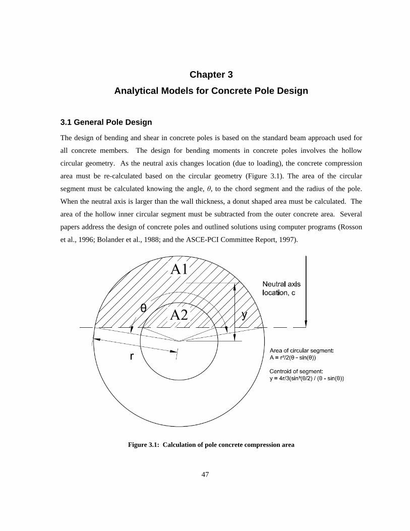
47

Chapter 3 Analytical Models for Concrete Pole Design

3.1 General Pole Design

The design of bending and shear in concrete poles is based on the standard beam approach used for

all concrete members. The design for bending moments in concrete poles involves the hollow

circular geometry. As the neutral axis changes location (due to loading), the concrete compression

area must be re-calculated based on the circular geometry (Figure 3.1). The area of the circular

segment must be calculated knowing the angle, θ, to the chord segment and the radius of the pole.

When the neutral axis is larger than the wall thickness, a donut shaped area must be calculated. The

area of the hollow inner circular segment must be subtracted from the outer concrete area. Several

papers address the design of concrete poles and outlined solutions using computer programs (Rosson

et al., 1996; Bolander et al., 1988; and the ASCE-PCI Committee Report, 1997).

Figure 3.1: Calculation of pole concrete compression area

48

To aid in the analysis of the concrete pole specimens, a MatLab program was created to calculate

the bending resistance of prestressed concrete poles. The program was based on the papers by

Rosson et al. (1996), Bolander et al. (1988), and the ASCE-PCI Committee Report on concrete pole

design (1997). The pole design experience of The Walter Fedy Partnership, a consulting company in

Kitchener, Ontario was also used as a starting point for the program. Using the design formulae and

values outlined in ACI-318-05 and CSA A23.3-04, the program can calculate the cracking moments

and ultimate moments from both codes. The program was then further developed to include shear

and torsional resistances and the ability to analyze the moment resistance about the longitudinal axis

at any reinforcement angle, κ (Figure 3.2). It was determined that the rotated geometry presented in

Figure 3.2 a) represents the critical moment design geometry for round poles (geometry Figure 3.2 b)

has slightly higher moment resistances).

a) b)

Figure 3.2: Rotated geometry of prestressing strands

3.2 Pole Capacity Calculation Program

A summary and flowchart (Figure 3.3) of the pole capacity calculation program is provided to

demonstrate how the program calculates the capacity of the concrete pole. The program’s results

were validated by comparison with a prestressed pole design completed by The Walter Fedy

Partnership.

49

Read Inputs

Select code analysis type

Start loop for rotation of cross section

Start loop for length increment of pole

Begin neutral axis locating loop

(assume initially that NA is at 1/3 of diameter)

Calculate stress in strands/bars

Calculate stress in concrete

Compression block (based

on codes)

Parabolic stress/strain distribution

(Hognestad)

Is Ttot = Ctot?

No

Adj

ust N

A lo

catio

n

Yes

Calculate Moment Resistance

Calculate Shear and Torsional Resistance

Last length increment of pole?

Last cross section

rotation?

No

No

Yes

Yes

End Program

Output results

Figure 3.3: Flowchart of Pole Capacity Calculation Program

50

Figu

re 3

.4:

Scre

ensh

ot o

f Pol

e C

apac

ity C

alcu

latio

n Pr

ogra

m

51

The analysis begins by reading the inputs from the graphical user interface (Figure 3.4). The user

can specify the geometric properties of the pole, the concrete/prestressing/reinforcing steel properties

and helical reinforcing amount and spacing. The analysis can be run using the compression block

theory as outlined in the ACI and CSA concrete codes or using Hognestad’s parabola for the concrete

stress-strain relationship. The user can also specify the analysis length increments, whether to

analyze a rotated cross section, and if unfactored or factored results are required. Plots of the

moment, shear, and torsion capacities along the length of the pole can also be selected to be

outputted.

The calculations begin by setting the factors of safety and constants (modulus of elasticity/rupture,

and ultimate concrete strain) according to either the ACI or CSA standards. At this stage, the

intervals for the length and cross section rotation analysis are also set. The cross section rotation loop

and the length increment loops are started and the capacity analysis process is initiated for one

increment and rotation.

First the location of each prestressing strand and steel reinforcement bar is calculated and the

distance, d, from the top of the section is stored. The neutral axis is calculated by trial and error. A

loop is initiated to find the neutral axis location (the initial first step is to assume a neutral axis of 1/3

the diameter from the compression side. Using the ultimate compressive strain value of concrete as

the initial point at the top of the section and drawing a line through the assumed neutral axis provides

a strain diagram for the calculation of stress in the concrete and steel. The stresses in the strands and

reinforcing bars are calculated based on this strain diagram and checked for yielding. The concrete

stresses are calculated using either the compression block theory or Hognestad’s parabolic stress-

strain relationship (presented below).

⎟⎟

⎠

⎞

⎜⎜

⎝

⎛⎟⎟⎠

⎞⎜⎜⎝

⎛−=

2'

22

oocff

εε

εε

(3-1)

where ε is the strain in the concrete, f’c is the concrete compressive strength, and 002.0=oε .

For the compression block theory the area of the concrete circular segments in the compression

zone are calculated and multiplied by the stress block to get the resulting compressive force. The

centroid of the circular segment and lever arm from the neutral axis is also determined to locate the

location of the resultant compression force on the cross section. Using the parabolic stress-strain

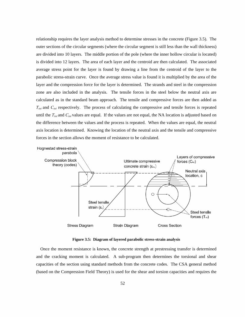
52

relationship requires the layer analysis method to determine stresses in the concrete (Figure 3.5). The

outer sections of the circular segments (where the circular segment is still less than the wall thickness)

are divided into 10 layers. The middle portion of the pole (where the inner hollow circular is located)

is divided into 12 layers. The area of each layer and the centroid are then calculated. The associated

average stress point for the layer is found by drawing a line from the centroid of the layer to the

parabolic stress-strain curve. Once the average stress value is found it is multiplied by the area of the

layer and the compression force for the layer is determined. The strands and steel in the compression

zone are also included in the analysis. The tensile forces in the steel below the neutral axis are

calculated as in the standard beam approach. The tensile and compressive forces are then added as

Ttot and Ctot respectively. The process of calculating the compressive and tensile forces is repeated

until the Ttot and Ctot values are equal. If the values are not equal, the NA location is adjusted based on

the difference between the values and the process is repeated. When the values are equal, the neutral

axis location is determined. Knowing the location of the neutral axis and the tensile and compressive

forces in the section allows the moment of resistance to be calculated.

Figure 3.5: Diagram of layered parabolic stress-strain analysis

Once the moment resistance is known, the concrete strength at prestressing transfer is determined

and the cracking moment is calculated. A sub-program then determines the torsional and shear

capacities of the section using standard methods from the concrete codes. The CSA general method

(based on the Compression Field Theory) is used for the shear and torsion capacities and requires the

53

use of a loop to iterate for the strain at midpoint of the section. The ACI method does not require the

loop. The sub-program returns the shear and torsional resistance values separated into the steel and

concrete contributions. Following the calculations for shear and torsion, the entire process of

calculating the moment capacity is repeated until the entire length of the pole has been analyzed. If

rotations of the cross section are selected by the user, the process is repeated again for the entire

length of the pole using the modified cross section layout. When all the iterations have been

completed the program outputs the capacity results in graphical and text format for moment, shear,

and torsion (Figure 3.6, Figure 3.7, and Figure 3.8).

0 2 4 6 8 10 125

10

15

20

25

30

35

40

45

50

55

Distance from Tip (m)

Mom

ent R

esis

tanc

e (k

N-m

)

Moment Resistance for a Round Pole

Mr CSAMcr CSAMn ACIMcr ACI

Figure 3.6: Moment resistance output from pole program

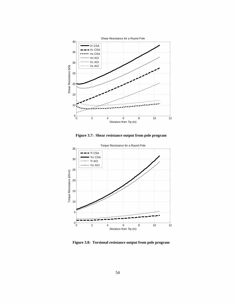
54

0 2 4 6 8 10 125

10

15

20

25

30

35

40


She

ar R

esis

tanc

e (k

N)

Shear Resistance for a Round Pole

Vr CSAVc CSAVs CSAVn ACIVc ACIVs ACI

Figure 3.7: Shear resistance output from pole program

0 2 4 6 8 10 120

5

10

15

20

25

30

35


Torq

ue R

esis

tanc

e (k

N-m

)

Torque Resistance for a Round Pole

Tr CSATcr CSATr ACITcr ACI

Figure 3.8: Torsional resistance output from pole program

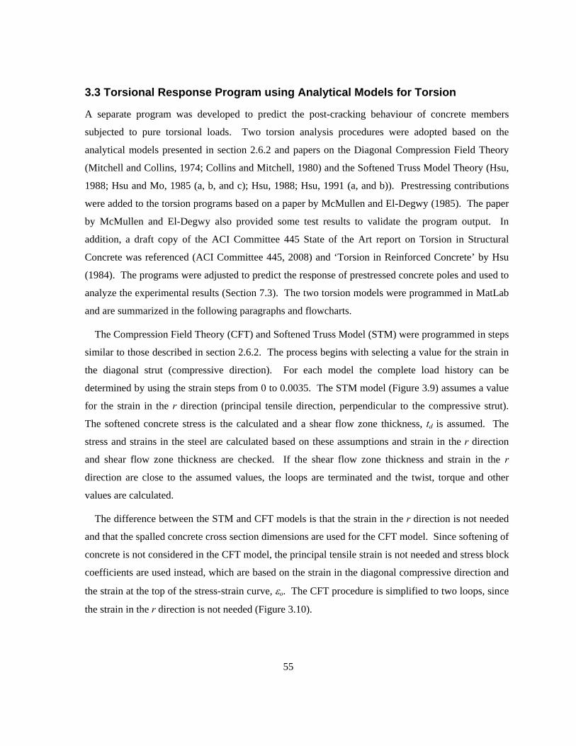
55

3.3 Torsional Response Program using Analytical Models for Torsion

A separate program was developed to predict the post-cracking behaviour of concrete members

subjected to pure torsional loads. Two torsion analysis procedures were adopted based on the

analytical models presented in section 2.6.2 and papers on the Diagonal Compression Field Theory

(Mitchell and Collins, 1974; Collins and Mitchell, 1980) and the Softened Truss Model Theory (Hsu,

1988; Hsu and Mo, 1985 (a, b, and c); Hsu, 1988; Hsu, 1991 (a, and b)). Prestressing contributions

were added to the torsion programs based on a paper by McMullen and El-Degwy (1985). The paper

by McMullen and El-Degwy also provided some test results to validate the program output. In

addition, a draft copy of the ACI Committee 445 State of the Art report on Torsion in Structural

Concrete was referenced (ACI Committee 445, 2008) and ‘Torsion in Reinforced Concrete’ by Hsu

(1984). The programs were adjusted to predict the response of prestressed concrete poles and used to

analyze the experimental results (Section 7.3). The two torsion models were programmed in MatLab

and are summarized in the following paragraphs and flowcharts.

The Compression Field Theory (CFT) and Softened Truss Model (STM) were programmed in steps

similar to those described in section 2.6.2. The process begins with selecting a value for the strain in

the diagonal strut (compressive direction). For each model the complete load history can be

determined by using the strain steps from 0 to 0.0035. The STM model (Figure 3.9) assumes a value

for the strain in the r direction (principal tensile direction, perpendicular to the compressive strut).

The softened concrete stress is the calculated and a shear flow zone thickness, td is assumed. The

stress and strains in the steel are calculated based on these assumptions and strain in the r direction

and shear flow zone thickness are checked. If the shear flow zone thickness and strain in the r

direction are close to the assumed values, the loops are terminated and the twist, torque and other

values are calculated.

The difference between the STM and CFT models is that the strain in the r direction is not needed

and that the spalled concrete cross section dimensions are used for the CFT model. Since softening of

concrete is not considered in the CFT model, the principal tensile strain is not needed and stress block

coefficients are used instead, which are based on the strain in the diagonal compressive direction and

the strain at the top of the stress-strain curve, εo. The CFT procedure is simplified to two loops, since

the strain in the r direction is not needed (Figure 3.10).

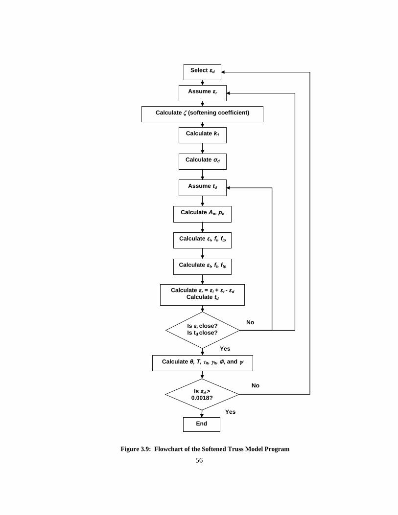
56

Select εd

Assume εr

Calculate ζ (softening coefficient)

Calculate k1

Calculate σd

Assume td

Calculate Ao, po

Calculate εl, fl, flp

Calculate εt, ft, ftp

Calculate εr = εl + εt - εd Calculate td

Is εr close?Is td close?

Calculate θ, T, τlt, γlt, Φ, and ψ

Is εd > 0.0018?

End

No

Yes

Yes

No

Figure 3.9: Flowchart of the Softened Truss Model Program

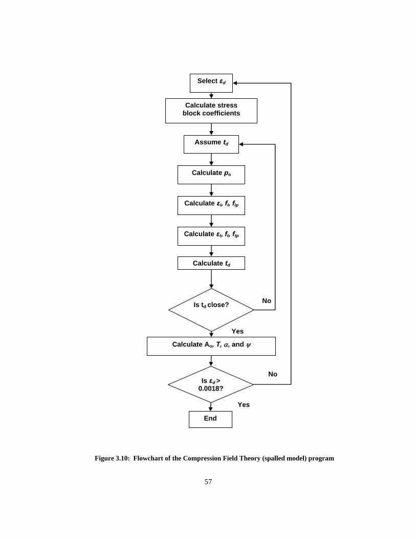
57

Select εd

Assume td

Calculate po

Calculate εl, fl, flp

Calculate εt, ft, ftp

Calculate td

Is td close?

Calculate Ao, T, α, and ψ

Is εd > 0.0018?

End

No

Yes

Yes

No

Calculate stress block coefficients

Figure 3.10: Flowchart of the Compression Field Theory (spalled model) program

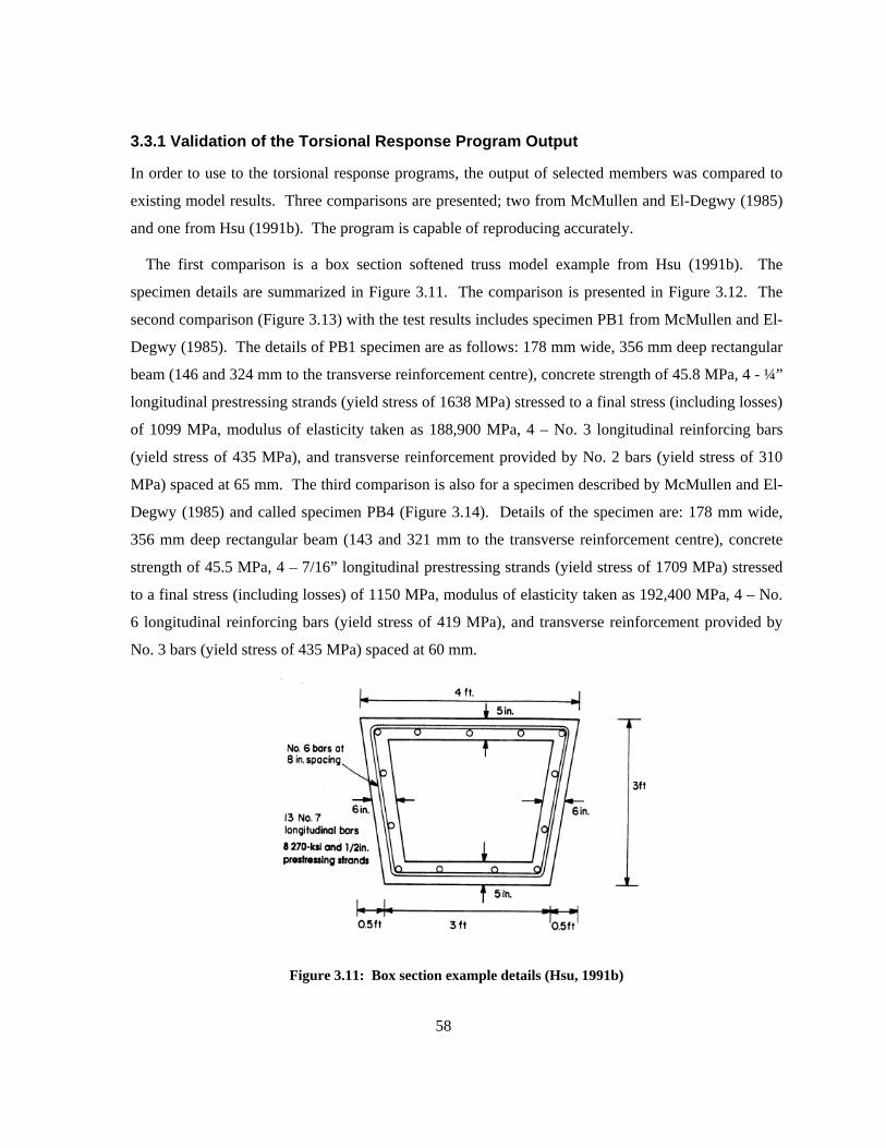
58

3.3.1 Validation of the Torsional Response Program Output

In order to use to the torsional response programs, the output of selected members was compared to

existing model results. Three comparisons are presented; two from McMullen and El-Degwy (1985)

and one from Hsu (1991b). The program is capable of reproducing accurately.

The first comparison is a box section softened truss model example from Hsu (1991b). The

specimen details are summarized in Figure 3.11. The comparison is presented in Figure 3.12. The

second comparison (Figure 3.13) with the test results includes specimen PB1 from McMullen and El-

Degwy (1985). The details of PB1 specimen are as follows: 178 mm wide, 356 mm deep rectangular

beam (146 and 324 mm to the transverse reinforcement centre), concrete strength of 45.8 MPa, 4 - ¼”

longitudinal prestressing strands (yield stress of 1638 MPa) stressed to a final stress (including losses)

of 1099 MPa, modulus of elasticity taken as 188,900 MPa, 4 – No. 3 longitudinal reinforcing bars

(yield stress of 435 MPa), and transverse reinforcement provided by No. 2 bars (yield stress of 310

MPa) spaced at 65 mm. The third comparison is also for a specimen described by McMullen and El-

Degwy (1985) and called specimen PB4 (Figure 3.14). Details of the specimen are: 178 mm wide,

356 mm deep rectangular beam (143 and 321 mm to the transverse reinforcement centre), concrete

strength of 45.5 MPa, 4 – 7/16” longitudinal prestressing strands (yield stress of 1709 MPa) stressed

to a final stress (including losses) of 1150 MPa, modulus of elasticity taken as 192,400 MPa, 4 – No.

6 longitudinal reinforcing bars (yield stress of 419 MPa), and transverse reinforcement provided by

No. 3 bars (yield stress of 435 MPa) spaced at 60 mm.

Figure 3.11: Box section example details (Hsu, 1991b)

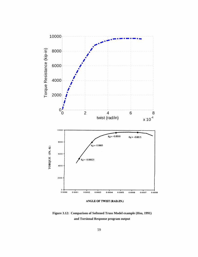
59

0 2 4 6 8x 10-4

0

2000

4000

6000

8000

10000

twist (rad/in)

Torq

ue R

esis

tanc

e (k

ip-in

)

Figure 3.12: Comparison of Softened Truss Model example (Hsu, 1991)

and Torsional Response program output

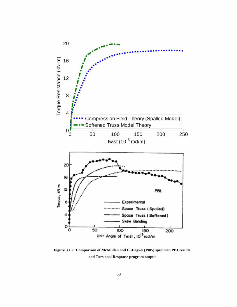
60

0 50 100 150 200 2500

4

8

12

16

20

twist (10-3 rad/m)

Torq

ue R

esis

tanc

e (k

N-m

)

Compression Field Theory (Spalled Model)Softened Truss Model Theory

Figure 3.13: Comparison of McMullen and El-Degwy (1985) specimen PB1 results


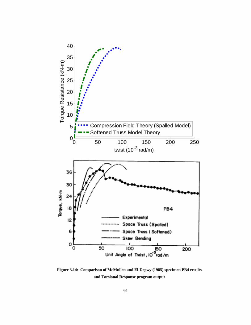
61

0 50 100 150 200 2500

5

10

15

20

25

30

35

40

twist (10-3 rad/m)

Torq

ue R

esis

tanc

e (k

N-m

)

Compression Field Theory (Spalled Model)Softened Truss Model Theory

Figure 3.14: Comparison of McMullen and El-Degwy (1985) specimen PB4 results


62

Chapter 4 Design of Test Program

4.1 General

A testing program was developed to determine the effect that helical reinforcement direction and

spacing (also referred to as pitch) have on the torsional response of prestressed concrete poles. A

total of 14 poles were produced with varying tip diameters, helical reinforcement directions, spacing,

and with single or double helical reinforcement. The specimens were produced by Sky Cast Inc. in

Guelph. Testing was also performed using the testing bed at Sky Cast Inc. with instrumentation from

the University of Waterloo, Civil and Environmental Engineering Department.

4.2 Experimental Program

The experimental program consisted of 14 Class C poles with differences in the direction of helical

steel and with varying spacing requirements. Two sizes of poles were produced, 165 mm tip

diameters and 210 mm tip diameters. For each size, three specimens were produced according to

CSA A14-07 (2007) standard. One specimen used a double helix (Figure 4.1 c)) to provide the

necessary percentage of helical reinforcement. The double helix consisted of two helixes, one wound

in each direction to form an overlapping system. The spacing of each half helix was governed by the

percentage of reinforcement required in the CSA code. The other two specimens, had a single helix

wound at half the spacing of the double helix halves. To achieve the same percentage of helical

reinforcement as the double helix using a single helix, the spacing of the reinforcement must be

reduced by half. The difference between the two specimens was that one had helical reinforcement

wound in the clockwise direction while the other was wound in the counter clockwise direction

(Figure 4.1). The poles in which the torsional load creates compressive principal stresses along the

direction of spirals is denoted as the counter clockwise direction (-CCW). The pole with the opposite

direction (with tensile torsional stresses along the spirals) is denoted as the clockwise direction (-

CW). Theoretically the counter clockwise reinforcement should be ineffective in resisting torque.

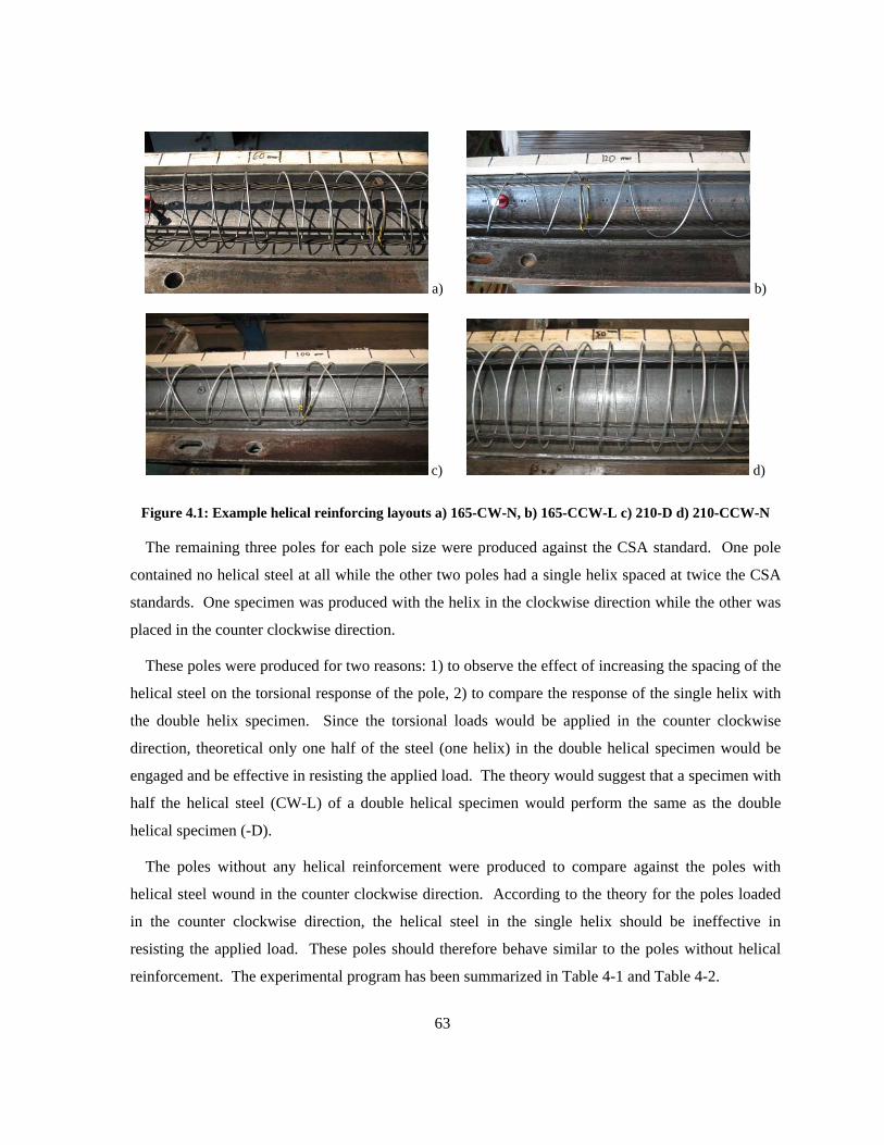
63

a) b)

c) d)

Figure 4.1: Example helical reinforcing layouts a) 165-CW-N, b) 165-CCW-L c) 210-D d) 210-CCW-N

The remaining three poles for each pole size were produced against the CSA standard. One pole

contained no helical steel at all while the other two poles had a single helix spaced at twice the CSA

standards. One specimen was produced with the helix in the clockwise direction while the other was

placed in the counter clockwise direction.

These poles were produced for two reasons: 1) to observe the effect of increasing the spacing of the

helical steel on the torsional response of the pole, 2) to compare the response of the single helix with

the double helix specimen. Since the torsional loads would be applied in the counter clockwise

direction, theoretical only one half of the steel (one helix) in the double helical specimen would be

engaged and be effective in resisting the applied load. The theory would suggest that a specimen with

half the helical steel (CW-L) of a double helical specimen would perform the same as the double

helical specimen (-D).

The poles without any helical reinforcement were produced to compare against the poles with

helical steel wound in the counter clockwise direction. According to the theory for the poles loaded

in the counter clockwise direction, the helical steel in the single helix should be ineffective in

resisting the applied load. These poles should therefore behave similar to the poles without helical

reinforcement. The experimental program has been summarized in Table 4-1 and Table 4-2.

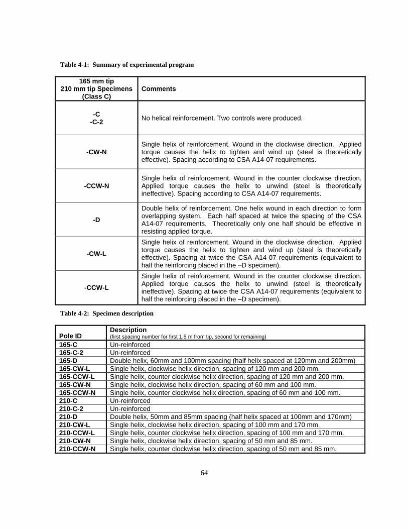
64

Table 4-1: Summary of experimental program

165 mm tip 210 mm tip Specimens

(Class C) Comments

-C -C-2 No helical reinforcement. Two controls were produced.

-CW-N Single helix of reinforcement. Wound in the clockwise direction. Applied torque causes the helix to tighten and wind up (steel is theoretically effective). Spacing according to CSA A14-07 requirements.

-CCW-N Single helix of reinforcement. Wound in the counter clockwise direction. Applied torque causes the helix to unwind (steel is theoretically ineffective). Spacing according to CSA A14-07 requirements.

-D Double helix of reinforcement. One helix wound in each direction to form overlapping system. Each half spaced at twice the spacing of the CSA A14-07 requirements. Theoretically only one half should be effective in resisting applied torque.

-CW-L Single helix of reinforcement. Wound in the clockwise direction. Applied torque causes the helix to tighten and wind up (steel is theoretically effective). Spacing at twice the CSA A14-07 requirements (equivalent to half the reinforcing placed in the –D specimen).

-CCW-L Single helix of reinforcement. Wound in the counter clockwise direction. Applied torque causes the helix to unwind (steel is theoretically ineffective). Spacing at twice the CSA A14-07 requirements (equivalent to half the reinforcing placed in the –D specimen).

Table 4-2: Specimen description

Pole ID Description (first spacing number for first 1.5 m from tip, second for remaining)

165-C Un-reinforced 165-C-2 Un-reinforced 165-D Double helix, 60mm and 100mm spacing (half helix spaced at 120mm and 200mm) 165-CW-L Single helix, clockwise helix direction, spacing of 120 mm and 200 mm. 165-CCW-L Single helix, counter clockwise helix direction, spacing of 120 mm and 200 mm. 165-CW-N Single helix, clockwise helix direction, spacing of 60 mm and 100 mm. 165-CCW-N Single helix, counter clockwise helix direction, spacing of 60 mm and 100 mm. 210-C Un-reinforced 210-C-2 Un-reinforced 210-D Double helix, 50mm and 85mm spacing (half helix spaced at 100mm and 170mm) 210-CW-L Single helix, clockwise helix direction, spacing of 100 mm and 170 mm. 210-CCW-L Single helix, counter clockwise helix direction, spacing of 100 mm and 170 mm. 210-CW-N Single helix, clockwise helix direction, spacing of 50 mm and 85 mm. 210-CCW-N Single helix, counter clockwise helix direction, spacing of 50 mm and 85 mm.

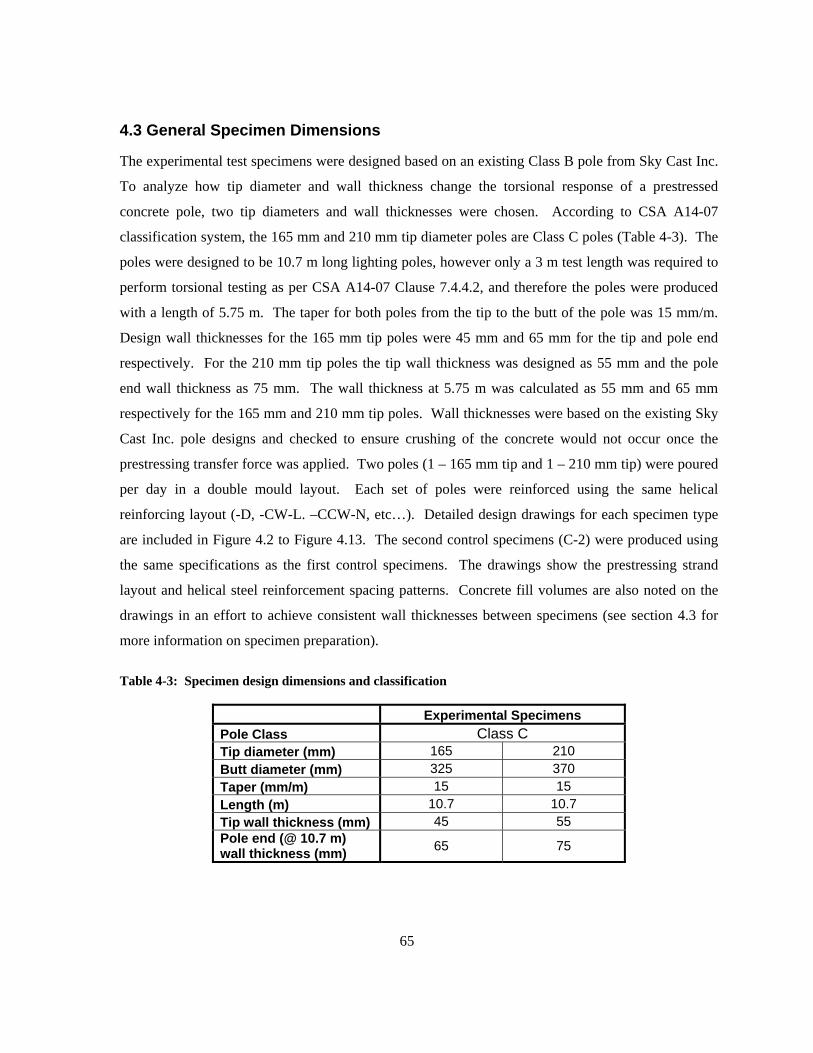
65

4.3 General Specimen Dimensions

The experimental test specimens were designed based on an existing Class B pole from Sky Cast Inc.

To analyze how tip diameter and wall thickness change the torsional response of a prestressed

concrete pole, two tip diameters and wall thicknesses were chosen. According to CSA A14-07

classification system, the 165 mm and 210 mm tip diameter poles are Class C poles (Table 4-3). The

poles were designed to be 10.7 m long lighting poles, however only a 3 m test length was required to

perform torsional testing as per CSA A14-07 Clause 7.4.4.2, and therefore the poles were produced

with a length of 5.75 m. The taper for both poles from the tip to the butt of the pole was 15 mm/m.

Design wall thicknesses for the 165 mm tip poles were 45 mm and 65 mm for the tip and pole end

respectively. For the 210 mm tip poles the tip wall thickness was designed as 55 mm and the pole

end wall thickness as 75 mm. The wall thickness at 5.75 m was calculated as 55 mm and 65 mm

respectively for the 165 mm and 210 mm tip poles. Wall thicknesses were based on the existing Sky

Cast Inc. pole designs and checked to ensure crushing of the concrete would not occur once the

prestressing transfer force was applied. Two poles (1 – 165 mm tip and 1 – 210 mm tip) were poured

per day in a double mould layout. Each set of poles were reinforced using the same helical

reinforcing layout (-D, -CW-L. –CCW-N, etc…). Detailed design drawings for each specimen type

are included in Figure 4.2 to Figure 4.13. The second control specimens (C-2) were produced using

the same specifications as the first control specimens. The drawings show the prestressing strand

layout and helical steel reinforcement spacing patterns. Concrete fill volumes are also noted on the

drawings in an effort to achieve consistent wall thicknesses between specimens (see section 4.3 for

more information on specimen preparation).

Table 4-3: Specimen design dimensions and classification

Experimental Specimens Pole Class Class C Tip diameter (mm) 165 210 Butt diameter (mm) 325 370 Taper (mm/m) 15 15 Length (m) 10.7 10.7 Tip wall thickness (mm) 45 55 Pole end (@ 10.7 m) wall thickness (mm) 65 75

66

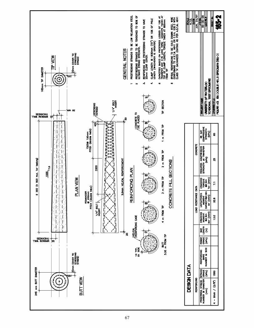
67

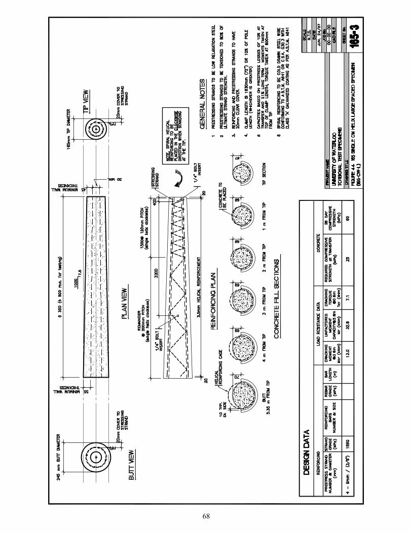
68

69

70

71

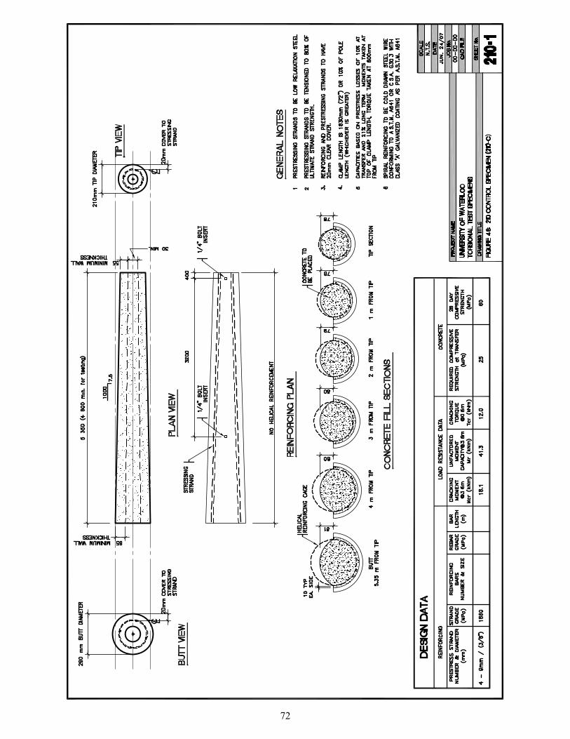
72

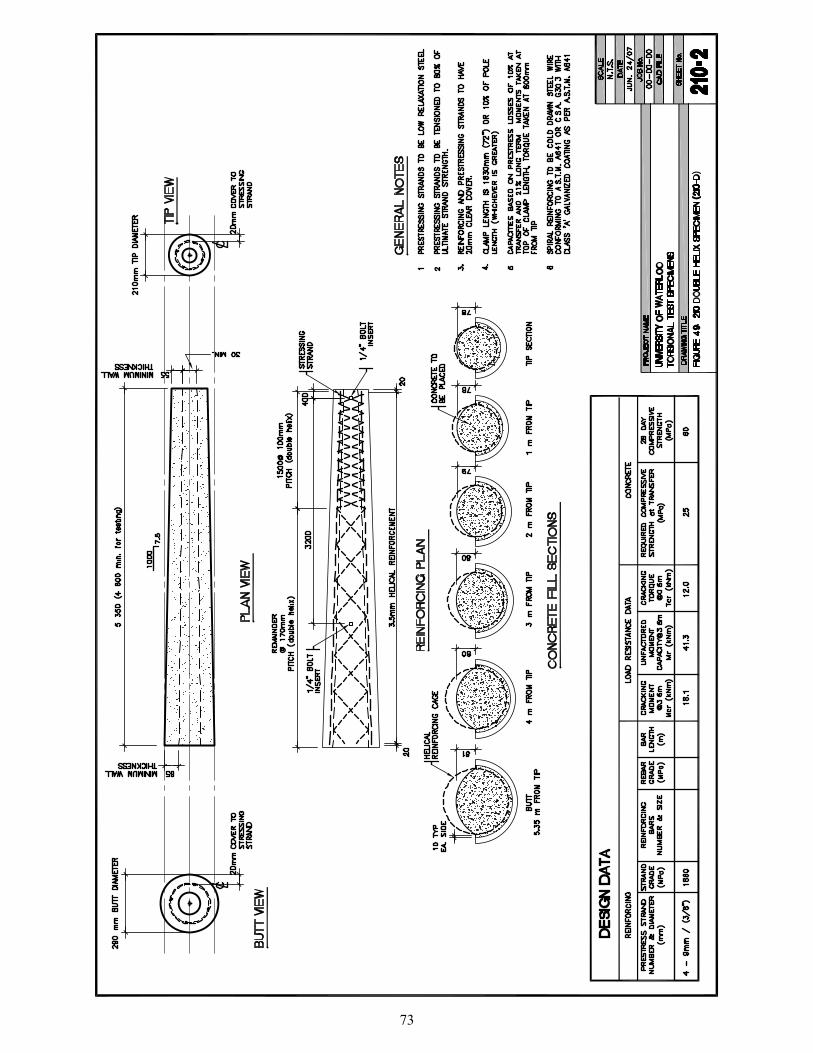
73

74

75

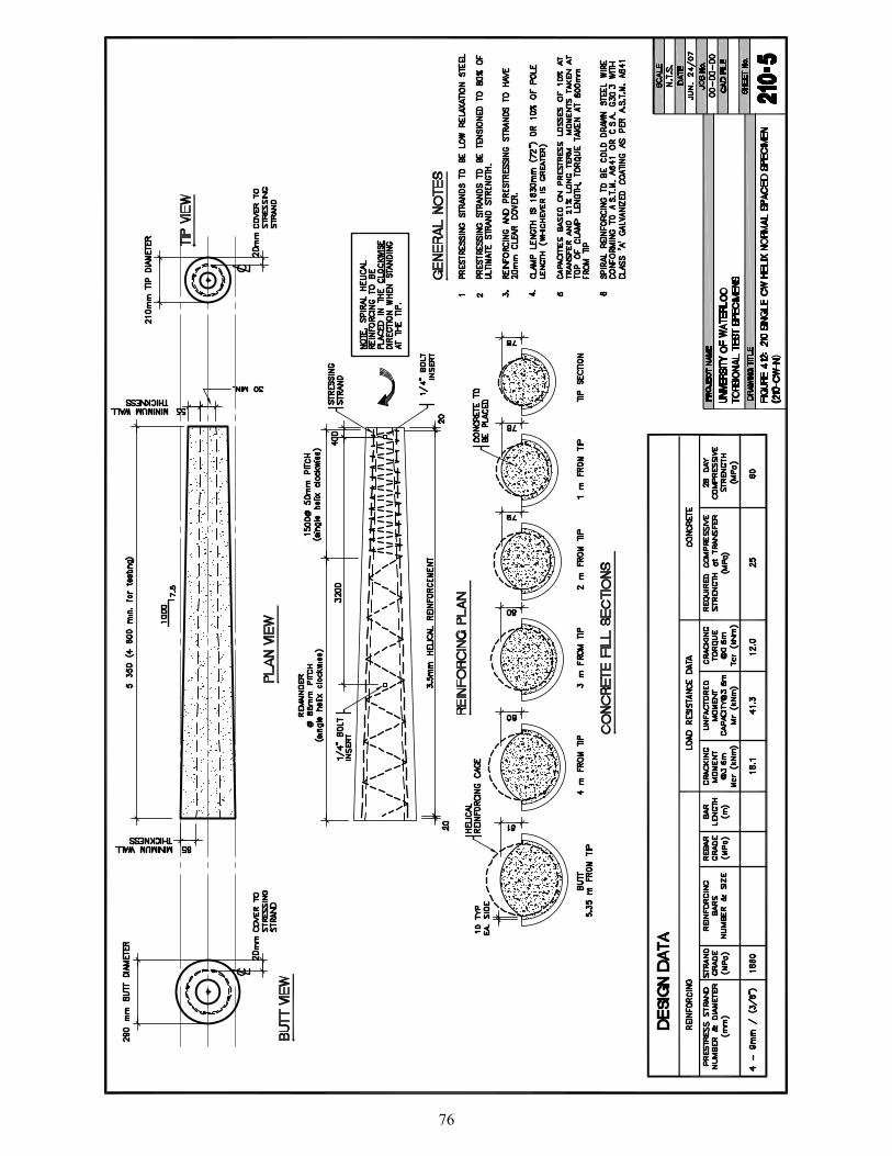
76

77

78

4.4 CSA A23.3-4 Specimen Design Moment, Shear and Torsion Values

The specimens were analyzed using the pole capacity analysis program presented in section 3.2.

According to the CSA A14-07 classification system a Class C pole is required to hold a 5.3 kN load

at 0.6 m from the tip. Typical ground embedment for concrete poles is 10 percent of the pole length

plus 2 feet (~ 0.66 m). For a 10.7 m design pole length, the corresponding classification ground line

moment at 9 m from the tip of the pole is 44.5 kN-m. The unfactored and factored design moment,

shear, and torsional capacities are given in Table 4-4 and Table 4-5 respectively. Comparing the

unfactored moments at 9 m from the tip to the required classification ground line moment confirms

that the specimens are all Class C poles.

Table 4-4: Calculated unfactored 165 and 210 specimen moment, shear, and torsional capacities

Specimen 165 Tip 210 Tip

Unfactored Resistances

Location (m from tip): 0.6 m 3.6 m 9 m 0.6 m 3.6 m 9 m

Mcr 13.0 23.2 18.1 30.7 Moment (kN-m) Mr 32.8 48.1 41.3 56.7 Vc 11.4 15.8 16.7 21.8 Vs 8.7 8.5 8.5 9.3 Shear (kN) Vr 20.1 24.3 25.2 31.1 Tcr 7.1 12.2 12.0 18.8 Torsion (kN-m) Tr 1.2 1.6 1.5 2.2

Transfer release strength (MPa) fci 25.2 16.2

Table 4-5: Calculated factored 165 and 210 specimen moment, shear, and torsional capacities

Specimen 165 Tip 210 Tip

Factored Resistances

Location (m from tip): 0.6 m 3.6 m 9 m 0.6 m 3.6 m 9 m

Mcr 13.0 23.2 18.1 30.7 Moment (kN-m) Mr 28.3 41.8 35.8 49.5 Vc 8.0 11.1 11.7 15.2 Vs 7.4 7.2 7.2 7.9 Shear (kN) Vr 15.4 19.3 18.9 23.1 Tcr 5.6 9.4 9.2 14.4 Torsion (kN-m) Tr 1.0 1.3 1.3 1.9

Transfer release strength (MPa) fci 25.2 16.2

79

The calculated ultimate torsion resistances are lower than the cracking torques in all cases since the

ultimate resistance is based on the transverse reinforcement alone. The concrete transfer release

strength required for the 165 mm specimens is 25.2 MPa and 16.2 MPa for the 210 mm specimens.

The shear capacity of the concrete is greater than the applied shear force indicating that the concrete

is adequate to resist the shear force. The output from the pole analysis program has been included in

Appendix A.

4.5 Specimen Preparation

The test specimens were produced by Sky Cast Inc. between August 22nd, 2007 and August 30th,

2007. The spun cast concrete pole production process is summarized in this section.

The moulds are first cleaned and then setup according to the Sky Cast specifications. The mould

design allows multiple mould sections to be assembled to produce a variety of pole lengths and

diameters. To save material costs the test specimens were produced shorter than normal poles at 5.345

m long, and therefore specially made wood tip and butt plates were fastened in the moulds at the

required diameters.

Once the setup of the mould is complete it is moved to the reinforcing and pouring stations. The

reinforcing and pouring steps in spun cast pole production uses the bottom half of the mould only.

Depending on the applied loads, 4 or 8 prestressing strands are spaced evenly within the pole section

and stressed initially to 20% of the final stressing to tighten the strands. The end plates on the mould

are left 3 to 5 mm away from the bottom mould half to allow enough room for the top mould to be

placed prior to the spinning process.

The helical reinforcing is wound by hand tightly against the stressing strands and spaced according

to the specifications of the pole (Figure 4.14). When a double helix of reinforcing is required an

additional coil is added in the opposite direction of the first. To ensure the required spacing of the

specimen helix was achieved for all specimens, a wooden ruler was used to indicate the spacing

needed (Figure 4.15). Typically the helical reinforcing is spaced by eye. The helical reinforcing is

typically a 3.5 mm cold drawn wire with a yield stress between 500 and 600 MPa (CSA A14-07).

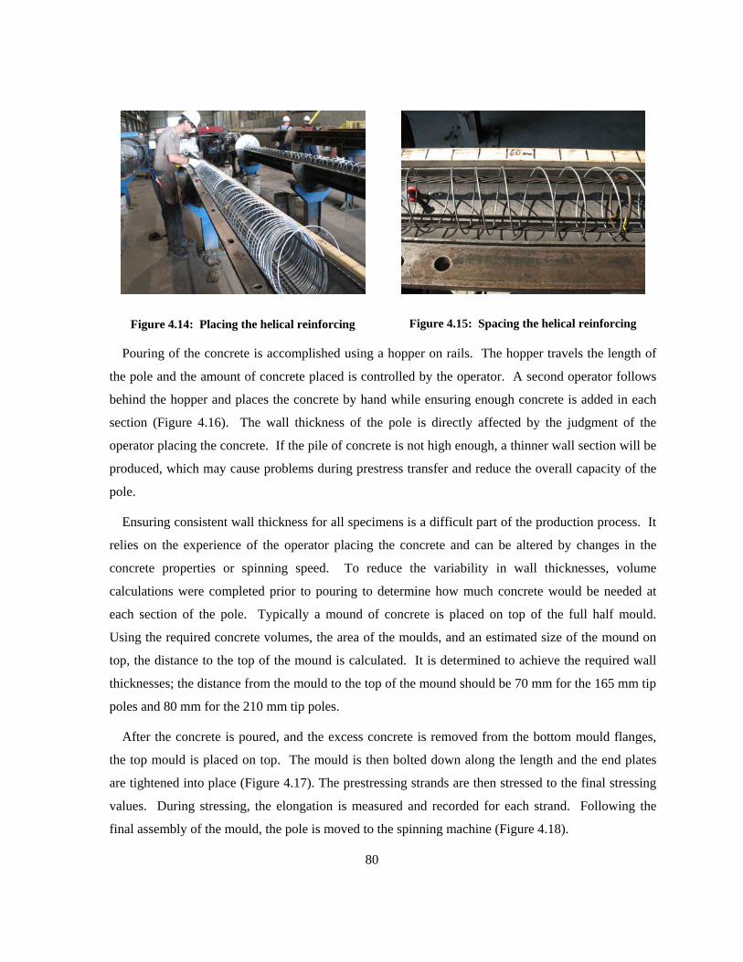
80

Figure 4.14: Placing the helical reinforcing

Figure 4.15: Spacing the helical reinforcing

Pouring of the concrete is accomplished using a hopper on rails. The hopper travels the length of

the pole and the amount of concrete placed is controlled by the operator. A second operator follows

behind the hopper and places the concrete by hand while ensuring enough concrete is added in each

section (Figure 4.16). The wall thickness of the pole is directly affected by the judgment of the

operator placing the concrete. If the pile of concrete is not high enough, a thinner wall section will be

produced, which may cause problems during prestress transfer and reduce the overall capacity of the

pole.

Ensuring consistent wall thickness for all specimens is a difficult part of the production process. It

relies on the experience of the operator placing the concrete and can be altered by changes in the

concrete properties or spinning speed. To reduce the variability in wall thicknesses, volume

calculations were completed prior to pouring to determine how much concrete would be needed at

each section of the pole. Typically a mound of concrete is placed on top of the full half mould.

Using the required concrete volumes, the area of the moulds, and an estimated size of the mound on

top, the distance to the top of the mound is calculated. It is determined to achieve the required wall

thicknesses; the distance from the mould to the top of the mound should be 70 mm for the 165 mm tip

poles and 80 mm for the 210 mm tip poles.

After the concrete is poured, and the excess concrete is removed from the bottom mould flanges,

the top mould is placed on top. The mould is then bolted down along the length and the end plates

are tightened into place (Figure 4.17). The prestressing strands are then stressed to the final stressing

values. During stressing, the elongation is measured and recorded for each strand. Following the

final assembly of the mould, the pole is moved to the spinning machine (Figure 4.18).

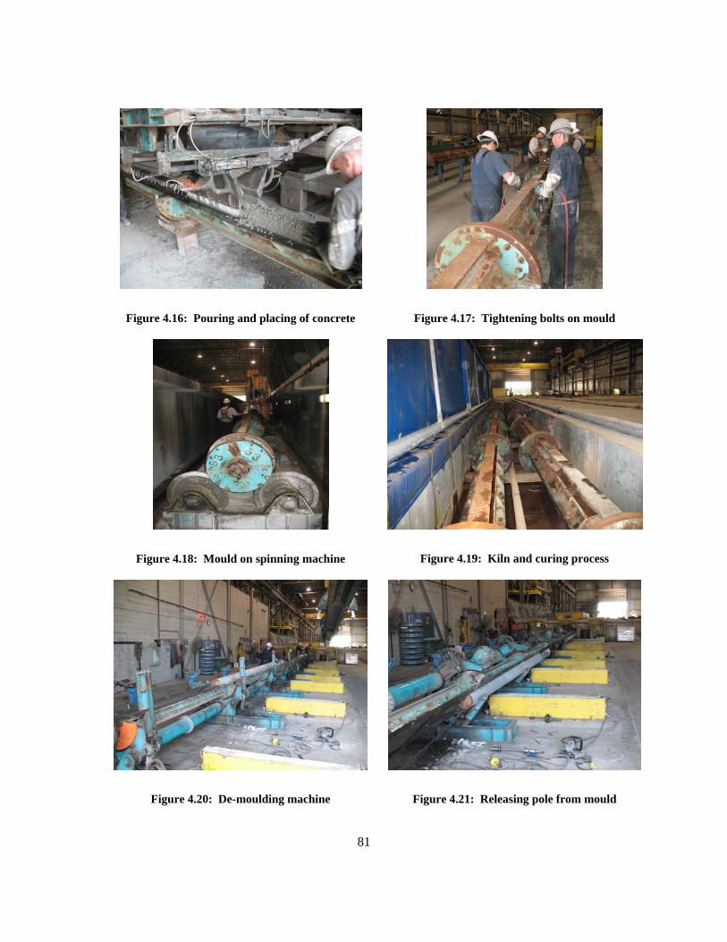
81

Figure 4.16: Pouring and placing of concrete

Figure 4.17: Tightening bolts on mould

Figure 4.18: Mould on spinning machine

Figure 4.19: Kiln and curing process

Figure 4.20: De-moulding machine

Figure 4.21: Releasing pole from mould

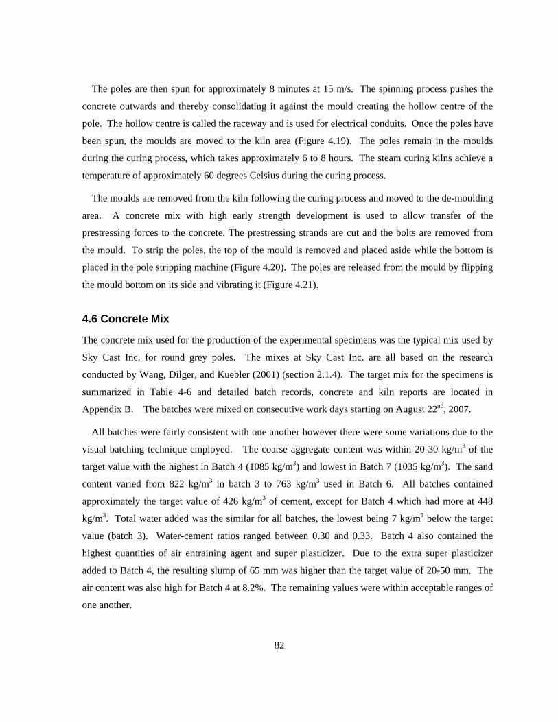
82

The poles are then spun for approximately 8 minutes at 15 m/s. The spinning process pushes the

concrete outwards and thereby consolidating it against the mould creating the hollow centre of the

pole. The hollow centre is called the raceway and is used for electrical conduits. Once the poles have

been spun, the moulds are moved to the kiln area (Figure 4.19). The poles remain in the moulds

during the curing process, which takes approximately 6 to 8 hours. The steam curing kilns achieve a

temperature of approximately 60 degrees Celsius during the curing process.

The moulds are removed from the kiln following the curing process and moved to the de-moulding

area. A concrete mix with high early strength development is used to allow transfer of the

prestressing forces to the concrete. The prestressing strands are cut and the bolts are removed from

the mould. To strip the poles, the top of the mould is removed and placed aside while the bottom is

placed in the pole stripping machine (Figure 4.20). The poles are released from the mould by flipping

the mould bottom on its side and vibrating it (Figure 4.21).

4.6 Concrete Mix

The concrete mix used for the production of the experimental specimens was the typical mix used by

Sky Cast Inc. for round grey poles. The mixes at Sky Cast Inc. are all based on the research

conducted by Wang, Dilger, and Kuebler (2001) (section 2.1.4). The target mix for the specimens is

summarized in Table 4-6 and detailed batch records, concrete and kiln reports are located in

Appendix B. The batches were mixed on consecutive work days starting on August 22nd, 2007.

All batches were fairly consistent with one another however there were some variations due to the

visual batching technique employed. The coarse aggregate content was within 20-30 kg/m3 of the

target value with the highest in Batch 4 (1085 kg/m3) and lowest in Batch 7 (1035 kg/m3). The sand

content varied from 822 kg/m3 in batch 3 to 763 kg/m3 used in Batch 6. All batches contained

approximately the target value of 426 kg/m3 of cement, except for Batch 4 which had more at 448

kg/m3. Total water added was the similar for all batches, the lowest being 7 kg/m3 below the target

value (batch 3). Water-cement ratios ranged between 0.30 and 0.33. Batch 4 also contained the

highest quantities of air entraining agent and super plasticizer. Due to the extra super plasticizer

added to Batch 4, the resulting slump of 65 mm was higher than the target value of 20-50 mm. The

air content was also high for Batch 4 at 8.2%. The remaining values were within acceptable ranges of

one another.

83

Table 4-6: Summary of target mix and actual specimen concrete mixes

Mix Targets Actual

Batch number (#): 1 2 - 7 1 (-C)

2 (-D)

3 (-C-2)

4 (-CCW-L)

5 (-CW-L)

6 (CW-N)

7 (CCW-N)

Batch size (m3) 0.38 0.46 0.38** 0.46 0.46 0.46 0.46 0.46 0.46 13 mm Coarse Aggregate (kg/m3)

1057 1045 1054 1048 1085 1052 1052 1035

Sand (kg/m3) 774 803 807 822 798 807 763 774

Type 30 HSF Cement (kg/m3)*

426 426 422 422 448 426 426 424

Total Water (kg/m3) 135 137 137 128 139 135 135 137

Air Entraining Agent (mL) 646 782 688 813 812 963 813 813 813 Super Plasticizer (mL) 2109 2553 2150 2600 2600 2650 2600 2600 2600 Water Reducing Agent (mL) 408 494 450 550 500 500 500 500 500 w/c ratio 0.32 0.32 0.33 0.30 0.31 0.32 0.32 0.32 Slump (mm) 20-50 35 35 40 65 55 55 45 Temperature ( °C) 25 minimum 25 27.5 28 28 28.5 28 27 Air Content (%) 5 - 8 4.8 6.1 6.7 8.2 6.4 6.5 6.6 Moisture Content (%) - 7 7.1 N/A 6.7 6.8 6.4 6.3 Fresh Density (kg/m3) - 2449 2391 2384 2354 2419 2427 2380 Kiln # 2 1 1 3 5 2 9 Average Curing Temperature over 4 hours ( °C)

60 +/- 5 62 61 61 59 59 61 54

Density of Hardened Concrete (kg/m3) - 2425 2394 2419 2321 2373 2395 2371

* = 82 % Type 30, 10 % silica fume, 8% slag ** = second batch made, more concrete was needed

4.6.1 Prestressing Strand

Each specimen was reinforced with 4 - 3/8” (9.5 mm) diameter prestressing strands spaced 90 degrees

around the pole cross section. The use of the same strand size for both poles allowed the double-pole

manufacturing process to be simplified since only one set of strands needed to be placed for two

poles. The prestressing strand had the following properties according to quality control test reports

(provided in Appendix B: Coil No. C-8944): area of 55.22 mm2, breaking load of 110.7 kN, yield

load of 102.3 kN, and modulus of elasticity of 199 534 MPa. The strands are initially stressed to 40%

of the final stressing force, which corresponds to 16.7 kN for the 3/8” strands. Afterwards, when final

stress values are applied, the resulting force is 80 kN for the 3/8” strands. The jacks used to stress the

prestressing strands are calibrated and stop when the design stressing stress of 80% fpu (1488 MPa,

resulting in 1176 MPa after 21% losses) is reached. Measurements of the strand elongation and tilt in

the end plates are typically taken between the initial and final stressing steps to confirm the stress in

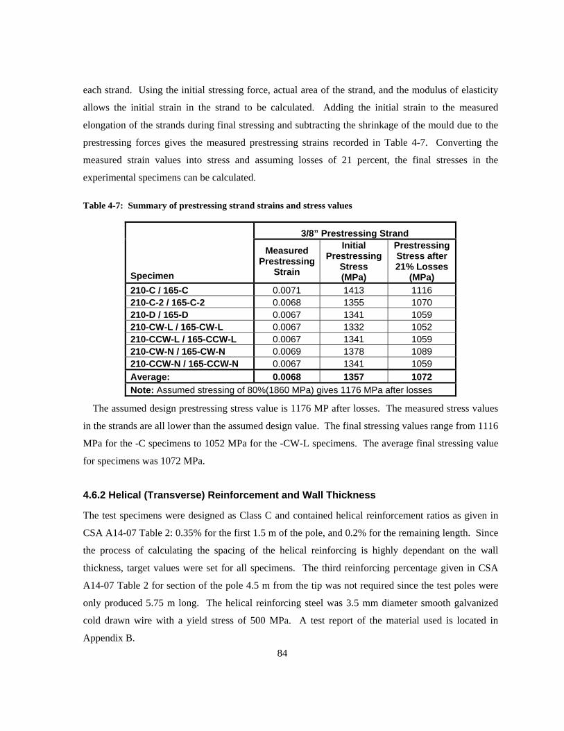
84

each strand. Using the initial stressing force, actual area of the strand, and the modulus of elasticity

allows the initial strain in the strand to be calculated. Adding the initial strain to the measured

elongation of the strands during final stressing and subtracting the shrinkage of the mould due to the

prestressing forces gives the measured prestressing strains recorded in Table 4-7. Converting the

measured strain values into stress and assuming losses of 21 percent, the final stresses in the

experimental specimens can be calculated.

Table 4-7: Summary of prestressing strand strains and stress values

3/8” Prestressing Strand

Specimen

Measured Prestressing

Strain

Initial Prestressing

Stress (MPa)

Prestressing Stress after 21% Losses

(MPa) 210-C / 165-C 0.0071 1413 1116 210-C-2 / 165-C-2 0.0068 1355 1070 210-D / 165-D 0.0067 1341 1059 210-CW-L / 165-CW-L 0.0067 1332 1052 210-CCW-L / 165-CCW-L 0.0067 1341 1059 210-CW-N / 165-CW-N 0.0069 1378 1089 210-CCW-N / 165-CCW-N 0.0067 1341 1059 Average: 0.0068 1357 1072 Note: Assumed stressing of 80%(1860 MPa) gives 1176 MPa after losses

The assumed design prestressing stress value is 1176 MP after losses. The measured stress values

in the strands are all lower than the assumed design value. The final stressing values range from 1116

MPa for the -C specimens to 1052 MPa for the -CW-L specimens. The average final stressing value

for specimens was 1072 MPa.

4.6.2 Helical (Transverse) Reinforcement and Wall Thickness

The test specimens were designed as Class C and contained helical reinforcement ratios as given in

CSA A14-07 Table 2: 0.35% for the first 1.5 m of the pole, and 0.2% for the remaining length. Since

the process of calculating the spacing of the helical reinforcing is highly dependant on the wall

thickness, target values were set for all specimens. The third reinforcing percentage given in CSA

A14-07 Table 2 for section of the pole 4.5 m from the tip was not required since the test poles were

only produced 5.75 m long. The helical reinforcing steel was 3.5 mm diameter smooth galvanized

cold drawn wire with a yield stress of 500 MPa. A test report of the material used is located in

Appendix B.

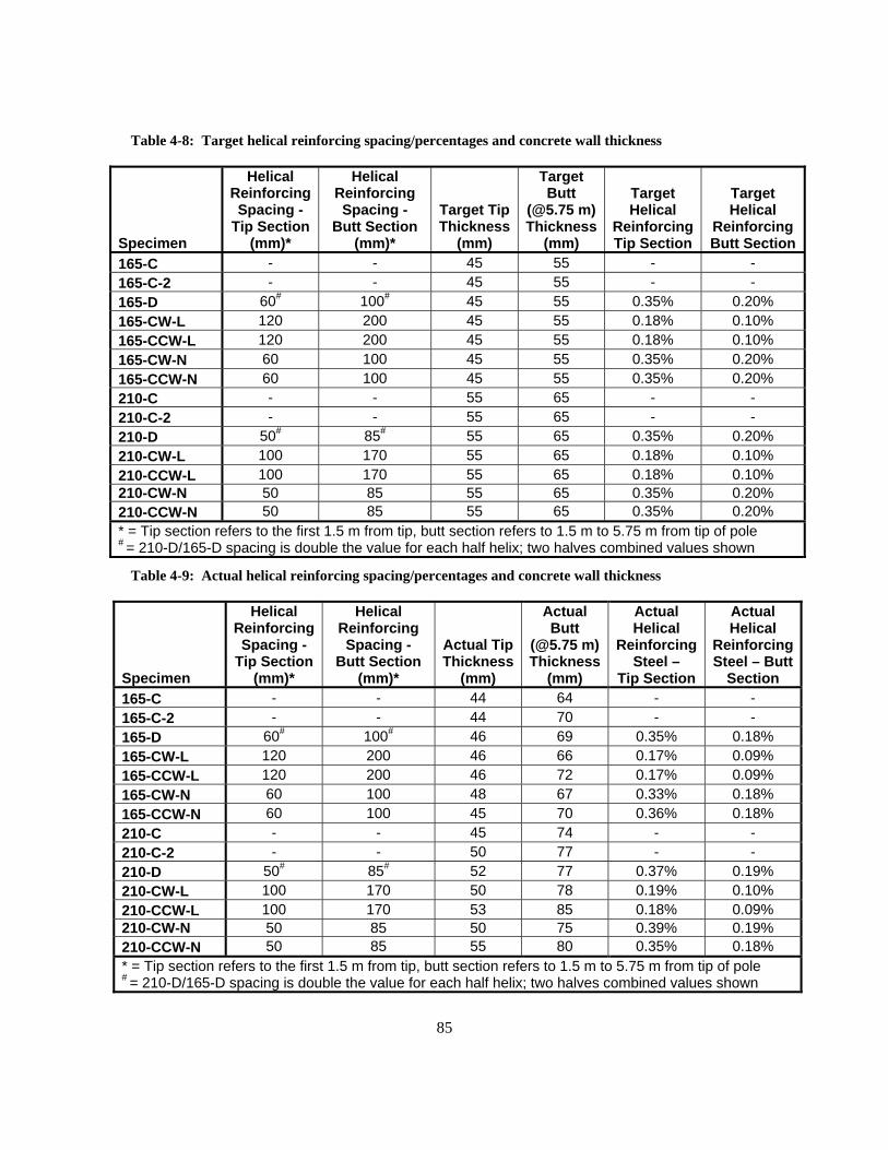
85

Table 4-8: Target helical reinforcing spacing/percentages and concrete wall thickness

Specimen

Helical Reinforcing Spacing -

Tip Section (mm)*


Butt Section (mm)*

Target Tip Thickness

(mm)

Target Butt

(@5.75 m)Thickness

(mm)

Target Helical

Reinforcing Tip Section

Target Helical

ReinforcingButt Section

165-C - - 45 55 - - 165-C-2 - - 45 55 - - 165-D 60# 100# 45 55 0.35% 0.20% 165-CW-L 120 200 45 55 0.18% 0.10% 165-CCW-L 120 200 45 55 0.18% 0.10% 165-CW-N 60 100 45 55 0.35% 0.20% 165-CCW-N 60 100 45 55 0.35% 0.20% 210-C - - 55 65 - - 210-C-2 - - 55 65 - - 210-D 50# 85# 55 65 0.35% 0.20% 210-CW-L 100 170 55 65 0.18% 0.10% 210-CCW-L 100 170 55 65 0.18% 0.10% 210-CW-N 50 85 55 65 0.35% 0.20% 210-CCW-N 50 85 55 65 0.35% 0.20% * = Tip section refers to the first 1.5 m from tip, butt section refers to 1.5 m to 5.75 m from tip of pole # = 210-D/165-D spacing is double the value for each half helix; two halves combined values shown

Table 4-9: Actual helical reinforcing spacing/percentages and concrete wall thickness

Specimen


Tip Section (mm)*


Butt Section (mm)*

Actual Tip Thickness

(mm)

Actual Butt

(@5.75 m)Thickness

(mm)

Actual Helical

Reinforcing Steel –

Tip Section

Actual Helical

Reinforcing Steel – Butt

Section 165-C - - 44 64 - - 165-C-2 - - 44 70 - - 165-D 60# 100# 46 69 0.35% 0.18% 165-CW-L 120 200 46 66 0.17% 0.09% 165-CCW-L 120 200 46 72 0.17% 0.09% 165-CW-N 60 100 48 67 0.33% 0.18% 165-CCW-N 60 100 45 70 0.36% 0.18% 210-C - - 45 74 - - 210-C-2 - - 50 77 - - 210-D 50# 85# 52 77 0.37% 0.19% 210-CW-L 100 170 50 78 0.19% 0.10% 210-CCW-L 100 170 53 85 0.18% 0.09% 210-CW-N 50 85 50 75 0.39% 0.19% 210-CCW-N 50 85 55 80 0.35% 0.18% * = Tip section refers to the first 1.5 m from tip, butt section refers to 1.5 m to 5.75 m from tip of pole # = 210-D/165-D spacing is double the value for each half helix; two halves combined values shown

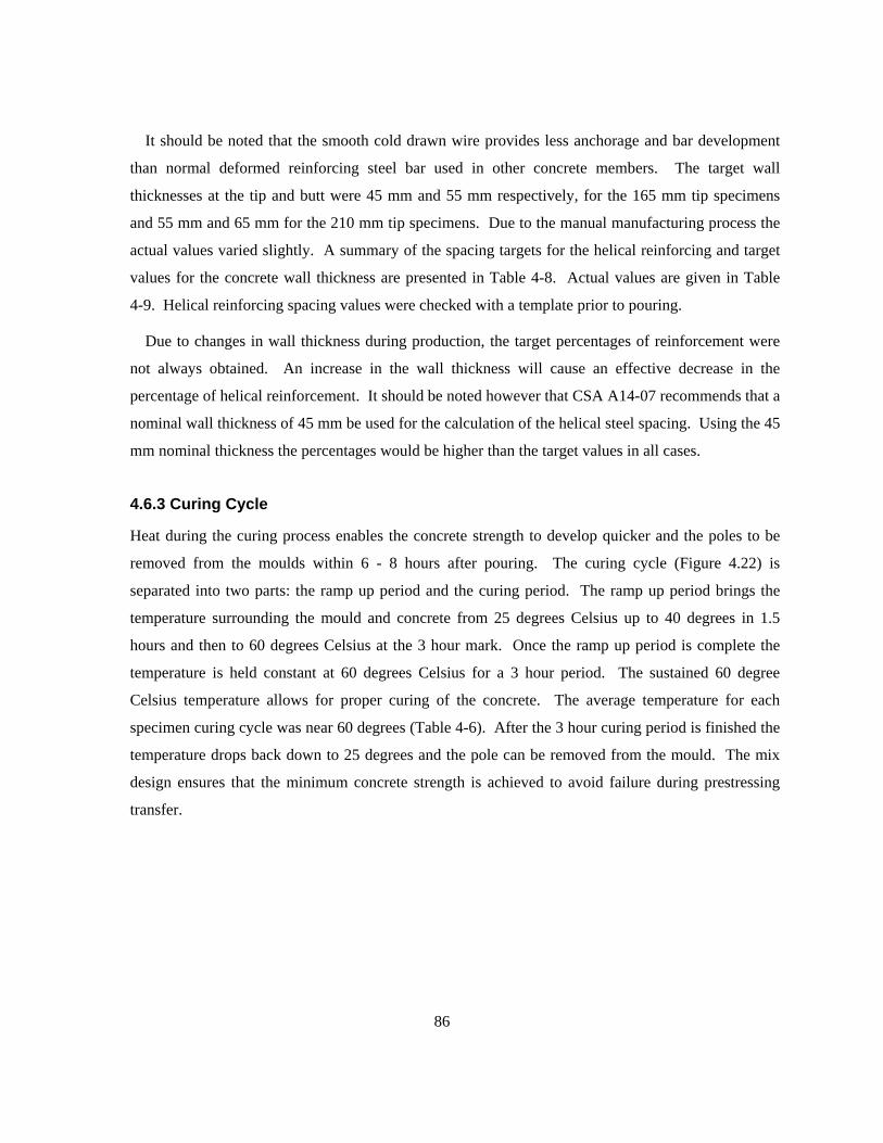
86

It should be noted that the smooth cold drawn wire provides less anchorage and bar development

than normal deformed reinforcing steel bar used in other concrete members. The target wall

thicknesses at the tip and butt were 45 mm and 55 mm respectively, for the 165 mm tip specimens

and 55 mm and 65 mm for the 210 mm tip specimens. Due to the manual manufacturing process the

actual values varied slightly. A summary of the spacing targets for the helical reinforcing and target

values for the concrete wall thickness are presented in Table 4-8. Actual values are given in Table

4-9. Helical reinforcing spacing values were checked with a template prior to pouring.

Due to changes in wall thickness during production, the target percentages of reinforcement were

not always obtained. An increase in the wall thickness will cause an effective decrease in the

percentage of helical reinforcement. It should be noted however that CSA A14-07 recommends that a

nominal wall thickness of 45 mm be used for the calculation of the helical steel spacing. Using the 45

mm nominal thickness the percentages would be higher than the target values in all cases.

4.6.3 Curing Cycle

Heat during the curing process enables the concrete strength to develop quicker and the poles to be

removed from the moulds within 6 - 8 hours after pouring. The curing cycle (Figure 4.22) is

separated into two parts: the ramp up period and the curing period. The ramp up period brings the

temperature surrounding the mould and concrete from 25 degrees Celsius up to 40 degrees in 1.5

hours and then to 60 degrees Celsius at the 3 hour mark. Once the ramp up period is complete the

temperature is held constant at 60 degrees Celsius for a 3 hour period. The sustained 60 degree

Celsius temperature allows for proper curing of the concrete. The average temperature for each

specimen curing cycle was near 60 degrees (Table 4-6). After the 3 hour curing period is finished the

temperature drops back down to 25 degrees and the pole can be removed from the mould. The mix

design ensures that the minimum concrete strength is achieved to avoid failure during prestressing

transfer.

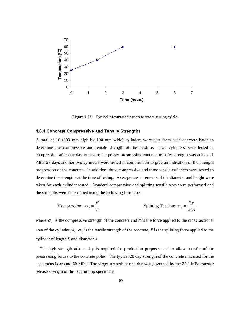
87

0

10

20

30

40

50

60

70

0 1 2 3 4 5 6 7

Time (hours)

Tem

pera

ture

(°C)

Figure 4.22: Typical prestressed concrete steam curing cylcle

4.6.4 Concrete Compressive and Tensile Strengths

A total of 16 (200 mm high by 100 mm wide) cylinders were cast from each concrete batch to

determine the compressive and tensile strength of the mixture. Two cylinders were tested in

compression after one day to ensure the proper prestressing concrete transfer strength was achieved.

After 28 days another two cylinders were tested in compression to give an indication of the strength

progression of the concrete. In addition, three compressive and three tensile cylinders were tested to

determine the strengths at the time of testing. Average measurements of the diameter and height were

taken for each cylinder tested. Standard compressive and splitting tensile tests were performed and

the strengths were determined using the following formulae:

Compression: AP

c =σ Splitting Tension: LdP

t πσ 2

=

where cσ is the compressive strength of the concrete and P is the force applied to the cross sectional

area of the cylinder, A, tσ is the tensile strength of the concrete, P is the splitting force applied to the

cylinder of length L and diameter d.

The high strength at one day is required for production purposes and to allow transfer of the

prestressing forces to the concrete poles. The typical 28 day strength of the concrete mix used for the

specimens is around 60 MPa. The target strength at one day was governed by the 25.2 MPa transfer

release strength of the 165 mm tip specimens.

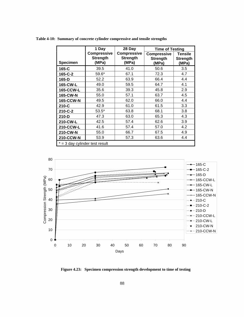
88

Table 4-10: Summary of concrete cylinder compressive and tensile strengths

Time of Testing

Specimen

1 Day Compressive

Strength (MPa)

28 Day Compressive

Strength (MPa)

Compressive Strength

(MPa)

Tensile Strength

(MPa) 165-C 39.5 41.0 50.6 3.5 165-C-2 59.6* 67.1 72.3 4.7 165-D 52.2 63.9 66.4 4.4 165-CW-L 49.0 59.5 64.7 4.1 165-CCW-L 35.6 39.3 45.8 2.9 165-CW-N 55.0 57.1 63.7 4.5 165-CCW-N 49.5 62.0 66.0 4.4 210-C 42.9 61.0 61.5 3.3 210-C-2 53.5* 63.8 68.1 3.8 210-D 47.3 63.0 65.3 4.3 210-CW-L 42.5 57.4 62.6 3.9 210-CCW-L 41.6 57.4 57.0 4.2 210-CW-N 55.0 66.7 67.5 4.9 210-CCW-N 53.9 57.3 63.6 4.4 * = 3 day cylinder test result

0

10

20

30

40

50

60

70

80

0 10 20 30 40 50 60 70 80 90Days

Com

pres

sion

Stre

ngth

(MP

a)

165-C165-C-2165-D165-CCW-L165-CW-L165-CW-N165-CCW-N210-C210-C-2210-D210-CCW-L210-CW-L210-CW-N210-CCW-N

Figure 4.23: Specimen compression strength development to time of testing

89

At one day, all specimens achieved the required transfer strength (Table 4-10). The strength at

prestressing transfer ranged from 35.6 to 59.6 MPa (three day result). Compression testing results at

28 days ranged from 39.3 MPa to 67.1 MPa (Table 4-10). The low value of the 165-CCW-L

specimen (39.3 MPa) can be traced to mix differences and variations in the kiln curing temperatures

from one end to the other. The CCW-L mixture could have been altered due to the higher air

entrainment and super plasticizer volume, which resulted in a higher slump. Only two specimens

(165-C and 165-CCW-L) had 28 day compression results well below the target 60 MPa concrete

strength. The remaining specimens had values over or just under the target concrete strength. At the

time of testing compressive strengths ranged from 45.8 MPa to 68.1 MPa. Tensile strengths ranged

from 2.9 MPa to 4.9 MPa. It should be noted that both the 165-C and 165-CCW-L specimens had

significantly lower values (~15-20 MPa) at the time of testing and may be reflected in their torsional

performance.

It should also be noted that even though the 165-CCW-L mix achieved the lowest concrete

strengths, the same mix used in the 210-CCW-L specimen achieved acceptable strengths. This

confirms the fact that variations in the kiln temperatures played a role in the strength development of

the concrete in the 165-CCW-L specimen. Figure 4.23 shows the compression strength development

of the specimens from the time of casting to the time of testing. All time of testing specimen

compression results, except the 165-C and 165-CCW-L specimens lie between 55 MPa and 72 MPa

and show similar strength development curves.

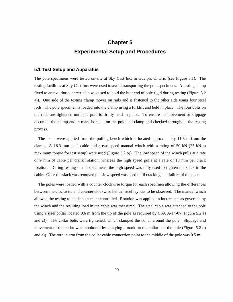
90

Chapter 5 Experimental Setup and Procedures

5.1 Test Setup and Apparatus

The pole specimens were tested on-site at Sky Cast Inc. in Guelph, Ontario (see Figure 5.1). The

testing facilities at Sky Cast Inc. were used to avoid transporting the pole specimens. A testing clamp

fixed to an exterior concrete slab was used to hold the butt end of pole rigid during testing (Figure 5.2

a)). One side of the testing clamp moves on rails and is fastened to the other side using four steel

rods. The pole specimen is loaded into the clamp using a forklift and held in place. The four bolts on

the rods are tightened until the pole is firmly held in place. To ensure no movement or slippage

occurs at the clamp end, a mark is made on the pole and clamp and checked throughout the testing

process.

The loads were applied from the pulling bench which is located approximately 11.5 m from the

clamp. A 16.3 mm steel cable and a two-speed manual winch with a rating of 50 kN (25 kN-m

maximum torque for test setup) were used (Figure 5.2 b)). The low speed of the winch pulls at a rate

of 9 mm of cable per crank rotation, whereas the high speed pulls at a rate of 18 mm per crack

rotation. During testing of the specimens, the high speed was only used to tighten the slack in the

cable. Once the slack was removed the slow speed was used until cracking and failure of the pole.

The poles were loaded with a counter clockwise torque for each specimen allowing the differences

between the clockwise and counter clockwise helical steel layouts to be observed. The manual winch

allowed the testing to be displacement controlled. Rotation was applied in increments as governed by

the winch and the resulting load in the cable was measured. The steel cable was attached to the pole

using a steel collar located 0.6 m from the tip of the pole as required by CSA A-14-07 (Figure 5.2 a)

and c)). The collar bolts were tightened, which clamped the collar around the pole. Slippage and

movement of the collar was monitored by applying a mark on the collar and the pole (Figure 5.2 d)

and e)). The torque arm from the collar cable connection point to the middle of the pole was 0.5 m.

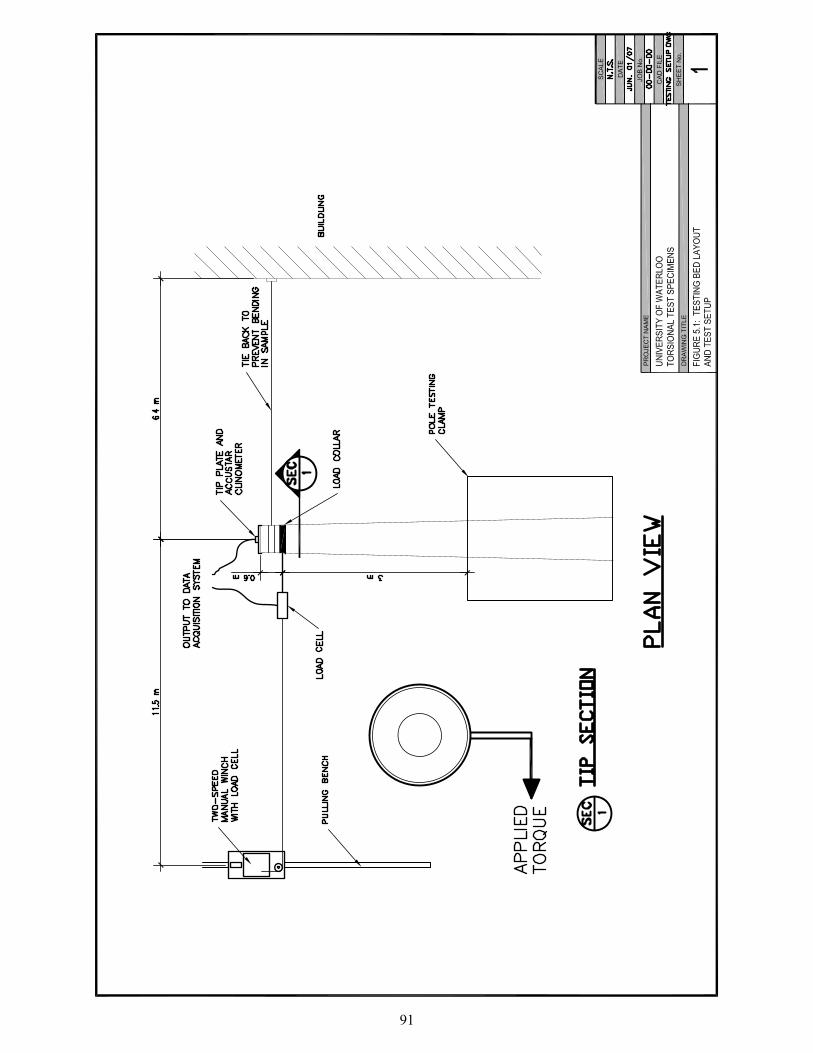
91

92

a) Pole testing clamp

b) Application of loads using two-speed manual winch

c) Loading and tie-back collar setup

d) monitoring movement at pole clamp end

e) monitoring movement at loading collar

Figure 5.2 a) - e): Pictures of test setup

93

To ensure pure torsional loads were applied to the specimens a tie back cable was attached to the

plant building (6.4 m in the opposite direction of the pulling bench). The tie back cable was tightened

using a griphoist and an 11 mm steel cable prior to testing. A loose steel collar was placed on the

pole near where the loading collar was fastened (Figure 5.2 c)).

Applied loads were recorded using a 44.5 kN (10000 lbs.) load cell attached between the loading

collar and the 16.3 mm steel cable. Twist values were recorded using an electronic clinometer

attached at the tip end of the pole.

5.2 Instrumentation

5.2.1 Data acquisition system

The data acquisition system consisted of a laptop, and a four input Onset HOBO micro station

datalogger. Two S-VIA-CM14 Onset 0-5 V adapters were used to input the applied load and twist

data values. The HOBO datalogger system was chosen as the data acquisition system since the

testing would be done onsite. A simple and easy to use system was needed to reduce the electronic

devices required on site. The data logger was easily launched using the HOBOware Pro software and

was downloaded to the laptop using a serial cable connection.

The use of the HOBO data loggers caused limitations on the data acquisition system. The 0-5 V

input adapters limited the input voltages from the instrumentation to 5 V. The HOBO data logger

could only record every 0.1 mV difference, and sample from the instrumentation every second. To

overcome these limitations the instrumentation output voltage was kept below 5 V and the loading

was applied slowly to ensure enough voltage values were recorded at each step.

5.2.2 Load Cells and Single Channel Signal Conditioner

Two load cells were used to record the applied loads. The first load cell was attached to the pulling

bench behind the winch to give the winch operator an indication of the load level. No data was

recorded from the first load cell.

The second load cell was placed between the steel cable and the load collar to obtain the most

accurate recording of the load applied to the pole specimen. The second load cell had a capacity of

44.5 kN (10000 lbs.) and an output of 3 mV/V. The load cell was excited with a 10.22 V signal.

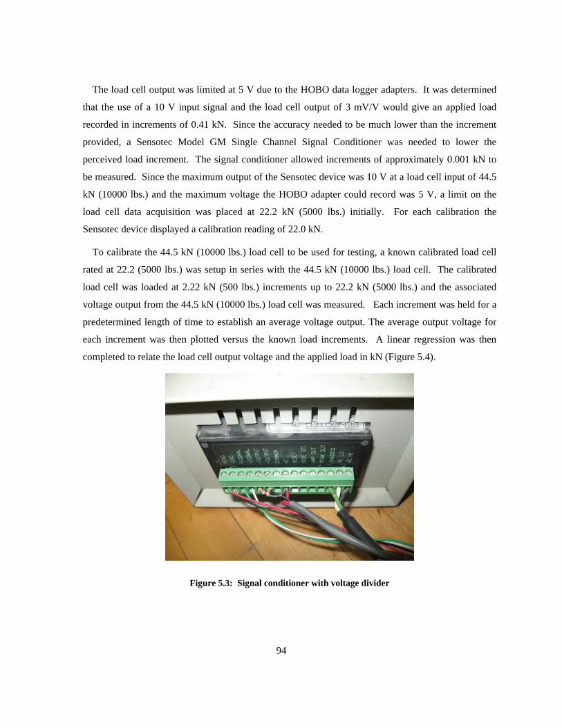
94

The load cell output was limited at 5 V due to the HOBO data logger adapters. It was determined

that the use of a 10 V input signal and the load cell output of 3 mV/V would give an applied load

recorded in increments of 0.41 kN. Since the accuracy needed to be much lower than the increment

provided, a Sensotec Model GM Single Channel Signal Conditioner was needed to lower the

perceived load increment. The signal conditioner allowed increments of approximately 0.001 kN to

be measured. Since the maximum output of the Sensotec device was 10 V at a load cell input of 44.5

kN (10000 lbs.) and the maximum voltage the HOBO adapter could record was 5 V, a limit on the

load cell data acquisition was placed at 22.2 kN (5000 lbs.) initially. For each calibration the

Sensotec device displayed a calibration reading of 22.0 kN.

To calibrate the 44.5 kN (10000 lbs.) load cell to be used for testing, a known calibrated load cell

rated at 22.2 (5000 lbs.) was setup in series with the 44.5 kN (10000 lbs.) load cell. The calibrated

load cell was loaded at 2.22 kN (500 lbs.) increments up to 22.2 kN (5000 lbs.) and the associated

voltage output from the 44.5 kN (10000 lbs.) load cell was measured. Each increment was held for a

predetermined length of time to establish an average voltage output. The average output voltage for

each increment was then plotted versus the known load increments. A linear regression was then

completed to relate the load cell output voltage and the applied load in kN (Figure 5.4).

Figure 5.3: Signal conditioner with voltage divider

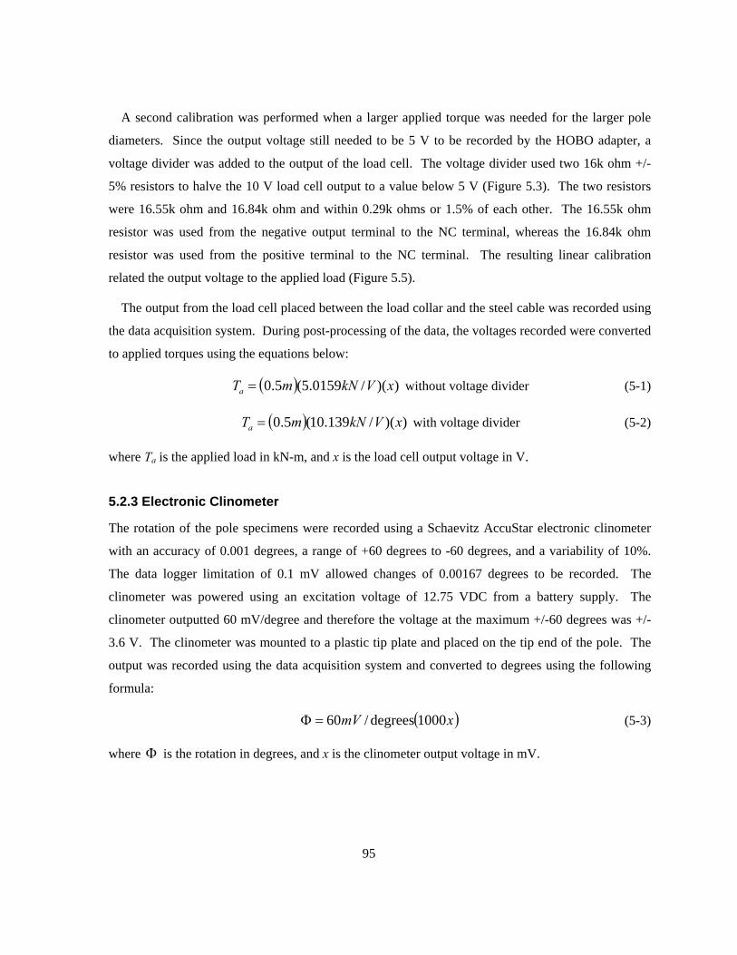
95

A second calibration was performed when a larger applied torque was needed for the larger pole

diameters. Since the output voltage still needed to be 5 V to be recorded by the HOBO adapter, a

voltage divider was added to the output of the load cell. The voltage divider used two 16k ohm +/-

5% resistors to halve the 10 V load cell output to a value below 5 V (Figure 5.3). The two resistors

were 16.55k ohm and 16.84k ohm and within 0.29k ohms or 1.5% of each other. The 16.55k ohm

resistor was used from the negative output terminal to the NC terminal, whereas the 16.84k ohm

resistor was used from the positive terminal to the NC terminal. The resulting linear calibration

related the output voltage to the applied load (Figure 5.5).

The output from the load cell placed between the load collar and the steel cable was recorded using

the data acquisition system. During post-processing of the data, the voltages recorded were converted

to applied torques using the equations below:

( ) ))(/0159.5(5.0 xVkNmTa = without voltage divider (5-1)

( ) ))(/139.10(5.0 xVkNmTa = with voltage divider (5-2)

where Ta is the applied load in kN-m, and x is the load cell output voltage in V.

5.2.3 Electronic Clinometer

The rotation of the pole specimens were recorded using a Schaevitz AccuStar electronic clinometer

with an accuracy of 0.001 degrees, a range of +60 degrees to -60 degrees, and a variability of 10%.

The data logger limitation of 0.1 mV allowed changes of 0.00167 degrees to be recorded. The

clinometer was powered using an excitation voltage of 12.75 VDC from a battery supply. The

clinometer outputted 60 mV/degree and therefore the voltage at the maximum +/-60 degrees was +/-

3.6 V. The clinometer was mounted to a plastic tip plate and placed on the tip end of the pole. The

output was recorded using the data acquisition system and converted to degrees using the following

formula:

( )xmV 1000degrees/60=Φ (5-3)

where Φ is the rotation in degrees, and x is the clinometer output voltage in mV.

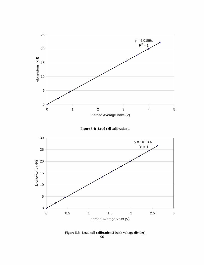
96

y = 5.0159xR2 = 1

0

5

10

15

20

25

0 1 2 3 4 5Zeroed Average Volts (V)

kilo

new

tons

(kN

)

Figure 5.4: Load cell calibration 1

y = 10.139xR2 = 1

0

5

10

15

20

25

30

0 0.5 1 1.5 2 2.5 3Zeroed Average Volts (V)

kilo

new

tons

(kN

)

Figure 5.5: Load cell calibration 2 (with voltage divider)

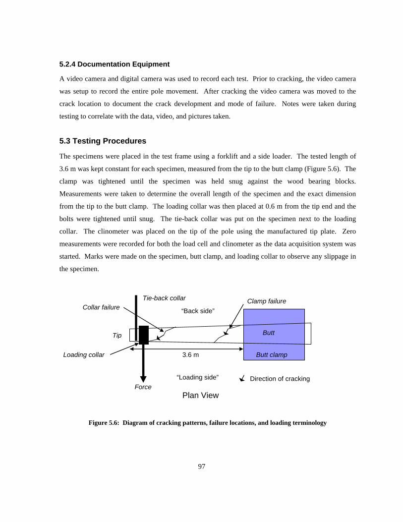
97

5.2.4 Documentation Equipment

A video camera and digital camera was used to record each test. Prior to cracking, the video camera

was setup to record the entire pole movement. After cracking the video camera was moved to the

crack location to document the crack development and mode of failure. Notes were taken during

testing to correlate with the data, video, and pictures taken.

5.3 Testing Procedures

The specimens were placed in the test frame using a forklift and a side loader. The tested length of

3.6 m was kept constant for each specimen, measured from the tip to the butt clamp (Figure 5.6). The

clamp was tightened until the specimen was held snug against the wood bearing blocks.

Measurements were taken to determine the overall length of the specimen and the exact dimension

from the tip to the butt clamp. The loading collar was then placed at 0.6 m from the tip end and the

bolts were tightened until snug. The tie-back collar was put on the specimen next to the loading

collar. The clinometer was placed on the tip of the pole using the manufactured tip plate. Zero

measurements were recorded for both the load cell and clinometer as the data acquisition system was

started. Marks were made on the specimen, butt clamp, and loading collar to observe any slippage in

the specimen.

Collar failure Clamp failure

“Loading side”

“Back side”

Butt clamp

Tie-back collar

Loading collar

ButtTip

Plan View

3.6 m

Force Direction of cracking

Figure 5.6: Diagram of cracking patterns, failure locations, and loading terminology

98

The load cell and the loading cable were then attached to the loading collar to begin testing of the

specimen. The load cell calibration shown in Figure 5.4 was used in testing of specimens 210-C,

210-C-2, and the pre-cracking portion of 210-D. Since the 210-D specimen required larger loads, the

load cell output was split using a voltage divider and the remaining 210 specimens and all of the 165

specimens were tested using the second calibration presented in Figure 5.5.

Since the load was applied manually, the best method for ensuring an approximate constant loading

rate was to have one person crank the winch slowly. The testing was performed in displacement

control mode using the two gears of the manual winch. After the cable slack was removed the low

speed of the winch was used, which pulled 9 mm of cable per full crank rotation. The loading rate

was difficult to maintain perfectly constant, however a rate of 0.7 degrees/min was calculated from

the data afterwards. As the specimen cracked and rotated, the cable slacked, meaning the slow crank

rotation allowed only the necessary amount of displacement and load to be applied. Load was applied

post-peak to record the behaviour after cracking. Specimen testing was completed once substantial

rotation occurred or the specimen fell to the ground. Measurements were also taken after testing to

determine the failure location, wall thickness, and cover to the prestressing steel.

99

Chapter 6 Experimental Results

6.1 Test Observations

Generally, the 165 specimens cracked and failed at the loading collar whereas the 210 specimens

began to fail at the butt clamp (Figure 5.6). Cracking was initiated on the back side for all specimens

and moved up towards the tip of the pole spiralling to the loading side of the specimen (Figure 5.6)

indicating that perhaps not all of the flexure was eliminated by the restraining cable. A summary of

the test results and observations are presented in Table 6-2 and Table 6-3. Specimens were tested in

the same order as presented in the following sections. The total length and tested specimen length

(distance from tip to clamp) were measured. Prior to each test the calibration of the electronic

equipment was checked and values for the excitation voltages for the load cell and clinometer, and the

Sensotec signal conditioner reading were recorded. Differences were noted between the excitation

voltages, and calibration readings. These differences can be contributed to the change in temperature

between tests and warming up of the electronic equipment. The recorded values for each specimen

have been summarized in Table 6-1. Raw test observation sheets are included in Appendix C.

Table 6-1: Summary of initial test excitation and calibration readings

Specimen Date and Time

Tested

Total Specimen

Length (m)

Tested Length

(m)

Excitation Voltage load cell

(V)

Sensotec Calibration

reading (kN)

Accustar Clinometer Excitation Voltage (V)

210-C Oct. 25, 10:30 AM 5.345 3.627 10.22 22.00 12.75 210-C-2 Oct. 30 11:01 AM 5.350 3.613 10.21 22.00 12.75 210-D Oct. 30 1:30 PM 5.350 3.605 10.22 21.95 12.75 210-CCW-L Nov. 6 10:55 AM 5.360 3.610 10.22 21.98 12.73 210-CW-L Nov. 6 11:55 AM 5.357 3.615 10.22 21.98 12.70 210-CCW-N Nov. 8 10:12 AM 5.350 3.622 10.22 21.97 12.74 210-CW-N Nov. 6 1:51 PM 5.347 3.608 10.22 22.03 12.69 165-C Nov. 8 11:15 AM 5.345 3.63 10.22 22.01 12.69 165-C-2 Nov. 8 12:07 PM 5.345 3.61 10.22 22.00 12.68 165-D Nov. 10 12:15 PM 5.350 3.608 10.22 21.99 12.73 165-CCW-L Nov. 13 10:35 AM 5.343 3.605 10.22 22.00 12.72 165-CW-L Nov. 13 11:35 AM 5.340 3.608 10.22 21.98 12.71 165-CW-N Nov. 13 1:45 PM 5.345 3.610 10.22 21.99 12.72 165-CCW-N Nov. 13 2:50 PM 5.344 3.604 10.22 22.00 12.71

100

After the maximum torque had been reached, loads were sustained to observe behaviour. The

behaviour was noted in the torque-twist figures when the curve looped back upon itself (Figure 6.3;

0.065 rad/m). The torque-twist loops can be attributed to increased cracking and movement in the

specimens. As an excess amount of torque is applied, the specimen releases energy post-peak

through rotation and increased cracking. The applied torque decreases suddenly causing slack in the

loading cable. The slack allows specimen relaxation and the torque-twist curve loop back behaviour.

6.1.1 Test Observations for 210 mm Tip Specimens

6.1.1.1 Specimen 210-C

The 210-C and 165-C specimens were the first to be produced. There was a shortage of concrete

during the production of the 210-C specimen which caused the wall thickness at the tip end of the

pole to be thinner on one side of the pole (Figure 6.1 a)). The cover from the inside wall of the pole

to the strand was only 5 to 10 mm. The wall thickness was only 45 mm, 10 mm thinner than the 55

mm needed. Due to the thinner wall and the lack of helical reinforcement in the 210-C control

specimen, a 400 mm longitudinal crack formed along the strand starting at the tip (Figure 6.1 b)).

Since the loading collar relies on friction resistance between the steel collar and the concrete pole,

slippage can occur if the bolts on the loading collar are not tightened adequately. Zero readings were

initially taken as 0.0006 V for the load cell, and 0.3961 V for the clinometer. Loading collar slippage

occurred at 10:48 AM and zero readings were re-established as 0.0006 V for the load cell and 0.3961

V for the clinometer.

The cracking torque of the specimen was determined from the torque-twist curve. Cracking of

210-C specimen occurred at 5.1 kN-m and a twist of 0.0011 rad/m. This corresponds to a stiffness of

4733.11 kN-m2/rad. Cracking was observed at the butt of the pole near the clamp. Ultimate torque

capacity of the specimen was 8.5 kN-m at 0.0029 rad/m of twist. Failure was sudden and brittle and

located at the butt clamp (Figure 6.1 c)). The failure crack extended 2.8 m from the butt clamp and

1.7 m into the clamped section. The bottom of the pole held in the clamp was cracked and large

pieces had spalled. Post failure, the specimen sustained approximately 1.5 kN-m. Large cracking and

twist deformation continued as the specimen continued to hold 1.5 – 2.0 kN-m load. Ultimately the

specimen fell to ground. The measured wall thickness at failure was 57 mm with a 20 mm cover to

the prestressing strands.

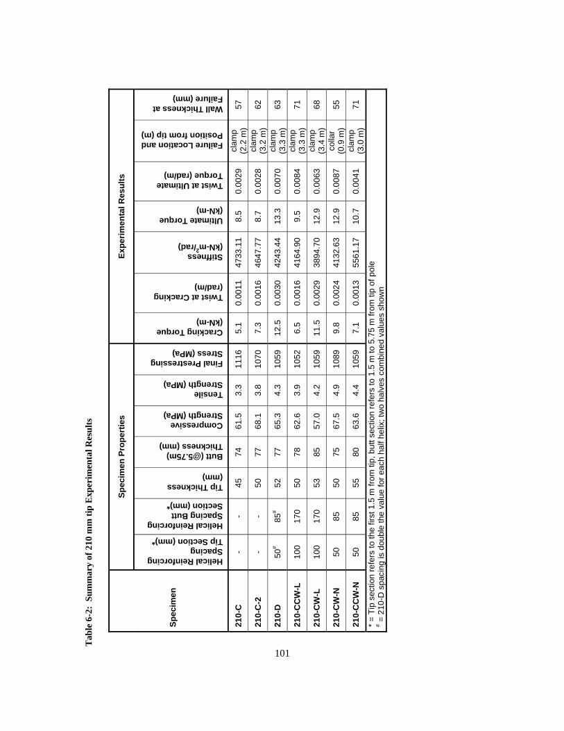
101

Tab

le 6

-2:

Sum

mar

y of

210

mm

tip

Exp

erim

enta

l Res

ults

Spec

imen

Pro

pert

ies

Expe

rimen

tal R

esul

ts

Spec

imen

Helical Reinforcing Spacing Tip Section (mm)*

Helical Reinforcing Spacing Butt Section (mm)*

Tip Thickness (mm)

Butt (@5.75m) Thickness (mm)

Compressive Strength (MPa)

Tensile Strength (MPa)

Final Prestressing Stress (MPa)

Cracking Torque (kN-m)

Twist at Cracking (rad/m)

Stiffness (kN-m

2/rad)

Ultimate Torque (kN-m)

Twist at Ultimate Torque (rad/m)

Failure Location and Position from tip (m)

Wall Thickness at Failure (mm)

210-

C

- -

45

74

61.5

3.

3 11

16

5.1

0.00

11

4733

.11

8.5

0.00

29

clam

p (2

.2 m

) 57

210-

C-2

-

- 50

77

68

.1

3.8

1070

7.

3 0.

0016

46

47.7

7 8.

7 0.

0028

cl

amp

(3

.2 m

) 62

210-

D

50#

85#

52

77

65.3

4.

3 10

59

12.5

0.

0030

42

43.4

4 13

.3

0.00

70

clam

p (3

.3 m

) 63

210-

CC

W-L

10

0 17

0 50

78

62

.6

3.9

1052

6.

5 0.

0016

41

64.9

0 9.

5 0.

0084

cl

amp

(3.3

m)

71

210-

CW

-L

100

170

53

85

57.0

4.

2 10

59

11.5

0.

0029

38

94.7

0 12

.9

0.00

63

clam

p (3

.4 m

) 68

210-

CW

-N

50

85

50

75

67.5

4.

9 10

89

9.8

0.00

24

4132

.63

12.9

0.

0087

co

llar

(0.9

m)

55

210-

CC

W-N

50

85

55

80

63

.6

4.4

1059

7.

1 0.

0013

55

61.1

7 10

.7

0.00

41

clam

p (3

.0 m

) 71

* = T

ip s

ectio

n re

fers

to th

e fir

st 1

.5 m

from

tip,

but

t sec

tion

refe

rs to

1.5

m to

5.7

5 m

from

tip

of p

ole

# = 2

10-D

spa

cing

is d

oubl

e th

e va

lue

for e

ach

half

helix

; tw

o ha

lves

com

bine

d va

lues

sho

wn

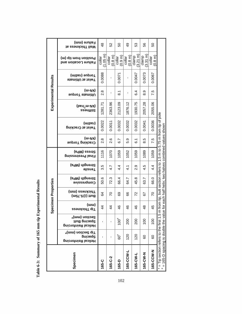
102

Tab

le 6

-3:

Sum

mar

y of

165

mm

tip

Exp

erim

enta

l Res

ults

Spec

imen

Pro

pert

ies

Expe

rimen

tal R

esul

ts

Spec

imen

Helical Reinforcing Spacing Tip Section (mm)*

Helical Reinforcing Spacing Butt Section (mm)*

Tip Thickness (mm)

Butt (@5.75m) Thickness (mm)

Compressive Strength (MPa)

Tensile Strength (MPa)

Final Prestressing Stress (MPa)

Cracking Torque (kN-m)

Twist at Cracking (rad/m)

Stiffness (kN-m

2/rad)

Ultimate Torque (kN-m)

Twist at Ultimate Torque (rad/m)

Failure Location and Position from tip (m)

Wall Thickness at Failure (mm)

165-

C

- -

44

64

50.6

3.

5 11

16

2.8

0.00

22

1281

.71

2.8

0.00

88

colla

r (1

.05

m)

48

165-

C-2

-

- 44

70

72

.3

4.7

1070

2.

6 0.

0011

23

63.9

6 -

- co

llar

(0.8

m)

52

165-

D

60#

100#

46

69

66.4

4.

4 10

59

6.7

0.00

32

2123

.09

8.1

0.00

71

colla

r (0

.9 m

) 50

165-

CC

W-L

12

0 20

0 46

66

64

.7

4.1

1052

5.

9 0.

0032

18

76.1

2 -

- co

llar

(0.8

m)

49

165-

CW

-L

120

200

46

72

45.8

2.

9 10

59

6.1

0.00

32

1930

.75

6.4

0.00

47

clam

p (3

.21

m)

53

165-

CW

-N

60

100

48

67

63.7

4.

5 10

89

8.5

0.00

41

2057

.28

8.9

0.00

73

clam

p (3

.31

m)

56

165-

CC

W-N

60

10

0 45

70

66

.0

4.4

1059

7.

5 0.

0036

20

55.0

6 7.

5 0.

0067

co

llar

(0.8

m)

50

* = T

ip s

ectio

n re

fers

to th

e fir

st 1

.5 m

from

tip,

but

t sec

tion

refe

rs to

1.5

m to

5.7

5 m

from

tip

of p

ole

# = 1

65-D

spa

cing

is d

oubl

e th

e va

lue

for e

ach

half

helix

; tw

o ha

lves

com

bine

d va

lues

sho

wn

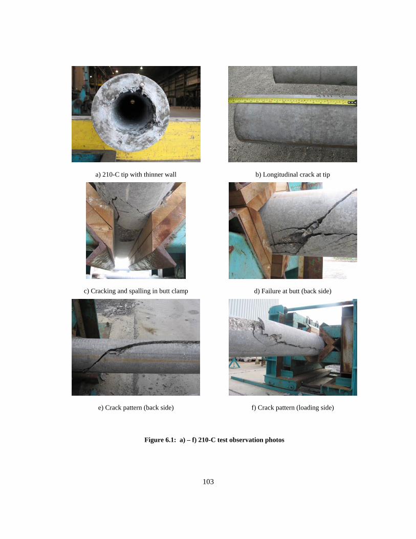
103

a) 210-C tip with thinner wall

b) Longitudinal crack at tip

c) Cracking and spalling in butt clamp

d) Failure at butt (back side)

e) Crack pattern (back side)

f) Crack pattern (loading side)

Figure 6.1: a) – f) 210-C test observation photos

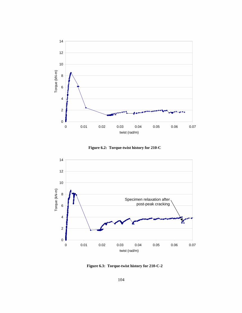
104

0

2

4

6

8

10

12

14

0 0.01 0.02 0.03 0.04 0.05 0.06 0.07twist (rad/m)

Torq

ue (k

N-m

)

Figure 6.2: Torque-twist history for 210-C

0

2

4

6

8

10

12

14

0 0.01 0.02 0.03 0.04 0.05 0.06 0.07twist (rad/m)

Torq

ue (k

N-m

)

Figure 6.3: Torque-twist history for 210-C-2

Specimen relaxation after post-peak cracking

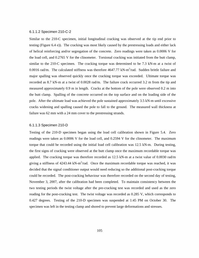
105

6.1.1.2 Specimen 210-C-2

Similar to the 210-C specimen, initial longitudinal cracking was observed at the tip end prior to

testing (Figure 6.4 e)). The cracking was most likely caused by the prestressing loads and either lack

of helical reinforcing and/or segregation of the concrete. Zero readings were taken as 0.0006 V for

the load cell, and 0.2765 V for the clinometer. Torsional cracking was initiated from the butt clamp,

similar to the 210-C specimen. The cracking torque was determined to be 7.3 kN-m at a twist of

0.0016 rad/m. The calculated stiffness was therefore 4647.77 kN-m2/rad. Sudden brittle failure and

major spalling was observed quickly once the cracking torque was exceeded. Ultimate torque was

recorded as 8.7 kN-m at a twist of 0.0028 rad/m. The failure crack occurred 3.2 m from the tip and

measured approximately 0.9 m in length. Cracks at the bottom of the pole were observed 0.2 m into

the butt clamp. Spalling of the concrete occurred on the top surface and on the loading side of the

pole. After the ultimate load was achieved the pole sustained approximately 3.5 kN-m until excessive

cracks widening and spalling caused the pole to fall to the ground. The measured wall thickness at

failure was 62 mm with a 24 mm cover to the prestressing strands.

6.1.1.3 Specimen 210-D

Testing of the 210-D specimen began using the load cell calibration shown in Figure 5.4. Zero

readings were taken as 0.0006 V for the load cell, and 0.2594 V for the clinometer. The maximum

torque that could be recorded using the initial load cell calibration was 12.5 kN-m. During testing,

the first signs of cracking were observed at the butt clamp once the maximum recordable torque was

applied. The cracking torque was therefore recorded as 12.5 kN-m at a twist value of 0.0030 rad/m

giving a stiffness of 4243.44 kN-m2/rad. Once the maximum recordable torque was reached, it was

decided that the signal conditioner output would need reducing so the additional post-cracking torque

could be recorded. The post-cracking behaviour was therefore recorded on the second day of testing,

November 3, 2007, after the calibration had been completed. To maintain consistency between the

two testing periods the twist voltage after the pre-cracking test was recorded and used as the zero

reading for the post-cracking test. The twist voltage was recorded as 0.285 V, which corresponds to

0.427 degrees. Testing of the 210-D specimen was suspended at 1:45 PM on October 30. The

specimen was left in the testing clamp and shored to prevent large deformations and stresses.

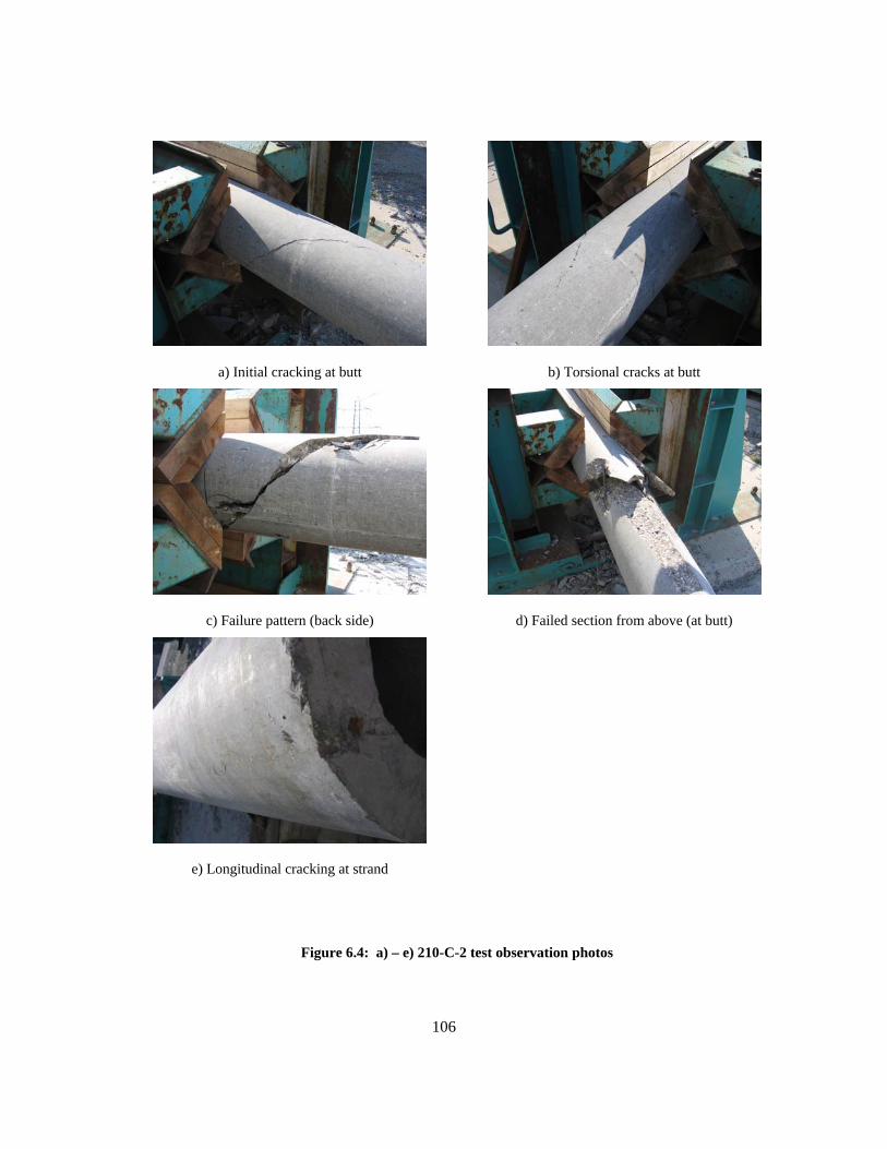
106

a) Initial cracking at butt

b) Torsional cracks at butt

c) Failure pattern (back side)

d) Failed section from above (at butt)

e) Longitudinal cracking at strand

Figure 6.4: a) – e) 210-C-2 test observation photos

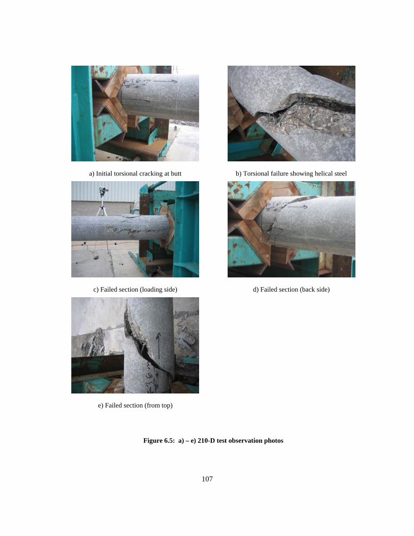
107

a) Initial torsional cracking at butt

b) Torsional failure showing helical steel

c) Failed section (loading side)

d) Failed section (back side)

e) Failed section (from top)

Figure 6.5: a) – e) 210-D test observation photos

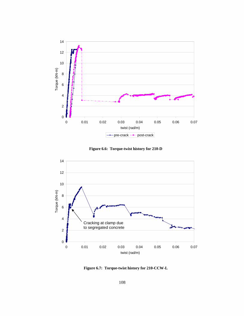
108

0

2

4

6

8

10

12

14

0 0.01 0.02 0.03 0.04 0.05 0.06 0.07twist (rad/m)

Torq

ue (k

N-m

)

pre-crack post-crack

Figure 6.6: Torque-twist history for 210-D

0

2

4

6

8

10

12

14

0 0.01 0.02 0.03 0.04 0.05 0.06 0.07twist (rad/m)

Torq

ue (k

N-m

)

Figure 6.7: Torque-twist history for 210-CCW-L

Cracking at clamp due to segregated concrete

109

Post-cracking testing for the 210-D specimen was continued on November 3 at 11:30 AM using the

load cell calibration as shown in Figure 5.5. The excitation voltage for the load cell was recorded as

10.22 V. The calibration reading from the Sensotec device was 21.98 kN. The battery providing

excitation to the AccuStar clinometer was outputting 12.75 V. Zero readings were taken as 0.0006 V

for the load cell, and 0.2863 V for the clinometer.

Due to the pre-cracked nature of the specimen a reduced stiffness was observed once loading was

continued. The post-cracking curve met the pre-cracking curve very closely indicating that post-

cracking testing would give acceptable torsional results. As the applied load was increased the crack

observed initially at the butt clamp continued to grow in size. Spalling, continued increase in crack

width, and yielding and necking of the helically steel was observed as the ultimate torque of 13.3 kN-

m was reached. The ultimate torque was found to occur at a twist of 0.0070 rad/m. Spalling occurred

0.8 m from the butt clamp, while the major crack causing failure was located at 3.3 m from the tip.

After the peak torque the specimen sustained 4 kN-m as the twist angle continually increased.

Spacing of the helical reinforcement in the failed portion was measured to be 100 mm. The measured

wall thickness at failure was 63 mm with a 30 mm cover to the prestressing strands.

6.1.1.4 Specimen 210-CCW-L

The zero readings for the 210-CCW-L specimen were taken as 0.0006 V for the load cell, and 0.4889

V for the clinometer. Cracking at the butt of the pole was observed at 6.5 kN-m and a twist of 0.0016

rad/m, giving a stiffness value of 4164.9 kN-m2/rad. Two cracks were observed at the butt of the

pole. One crack was located at the clamp, whereas the second crack formed approximately 200 mm

from the clamp. As the load was increased both cracks linked together, possibly due to additional

longitudinal cracking down the prestressing strand.

Increasing cracks widths near the butt of the pole and spalling of the concrete to 0.3 m from the

butt clamp (3.3 m from the tip) caused the failure of the specimen. Failure of the helical steel could

also be heard (popping sound) at this time. The ultimate torque was recorded as 9.5 kN-m at 0.0084

rad/m. Examination of the specimen after failure indicated that the helical steel did not arrest the

developing cracks. Instead, the cracks formed alongside the helical steel. Failure occurred when the

longitudinal cracking linked the torsional cracks together and caused a single piece of helical steel to

hold the load. Since the failure of the steel was heard at the same time as the specimen failed, it is

likely that the steel could not maintain the torsional load.

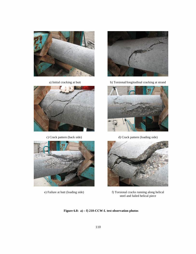
110


b) Torsional/longitudinal cracking at strand

c) Crack pattern (back side)

d) Crack pattern (loading side)

e) Failure at butt (loading side)

f) Torsional cracks running along helical steel and failed helical piece

Figure 6.8: a) – f) 210-CCW-L test observation photos

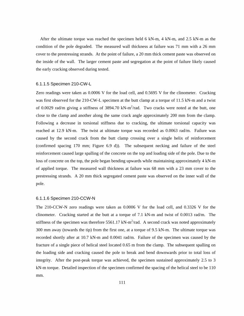
111

After the ultimate torque was reached the specimen held 6 kN-m, 4 kN-m, and 2.5 kN-m as the

condition of the pole degraded. The measured wall thickness at failure was 71 mm with a 26 mm

cover to the prestressing strands. At the point of failure, a 20 mm thick cement paste was observed on

the inside of the wall. The larger cement paste and segregation at the point of failure likely caused

the early cracking observed during tested.

6.1.1.5 Specimen 210-CW-L

Zero readings were taken as 0.0006 V for the load cell, and 0.5695 V for the clinometer. Cracking

was first observed for the 210-CW-L specimen at the butt clamp at a torque of 11.5 kN-m and a twist

of 0.0029 rad/m giving a stiffness of 3894.70 kN-m2/rad. Two cracks were noted at the butt, one

close to the clamp and another along the same crack angle approximately 200 mm from the clamp.

Following a decrease in torsional stiffness due to cracking, the ultimate torsional capacity was

reached at 12.9 kN-m. The twist at ultimate torque was recorded as 0.0063 rad/m. Failure was

caused by the second crack from the butt clamp crossing over a single helix of reinforcement

(confirmed spacing 170 mm; Figure 6.9 d)). The subsequent necking and failure of the steel

reinforcement caused large spalling of the concrete on the top and loading side of the pole. Due to the

loss of concrete on the top, the pole began bending upwards while maintaining approximately 4 kN-m

of applied torque. The measured wall thickness at failure was 68 mm with a 23 mm cover to the

prestressing strands. A 20 mm thick segregated cement paste was observed on the inner wall of the

pole.

6.1.1.6 Specimen 210-CCW-N

The 210-CCW-N zero readings were taken as 0.0006 V for the load cell, and 0.3326 V for the

clinometer. Cracking started at the butt at a torque of 7.1 kN-m and twist of 0.0013 rad/m. The

stiffness of the specimen was therefore 5561.17 kN-m2/rad. A second crack was noted approximately

300 mm away (towards the tip) from the first one, at a torque of 9.5 kN-m. The ultimate torque was

recorded shortly after at 10.7 kN-m and 0.0041 rad/m. Failure of the specimen was caused by the

fracture of a single piece of helical steel located 0.65 m from the clamp. The subsequent spalling on

the loading side and cracking caused the pole to break and bend downwards prior to total loss of

integrity. After the post-peak torque was achieved, the specimen sustained approximately 2.5 to 3

kN-m torque. Detailed inspection of the specimen confirmed the spacing of the helical steel to be 110

mm.

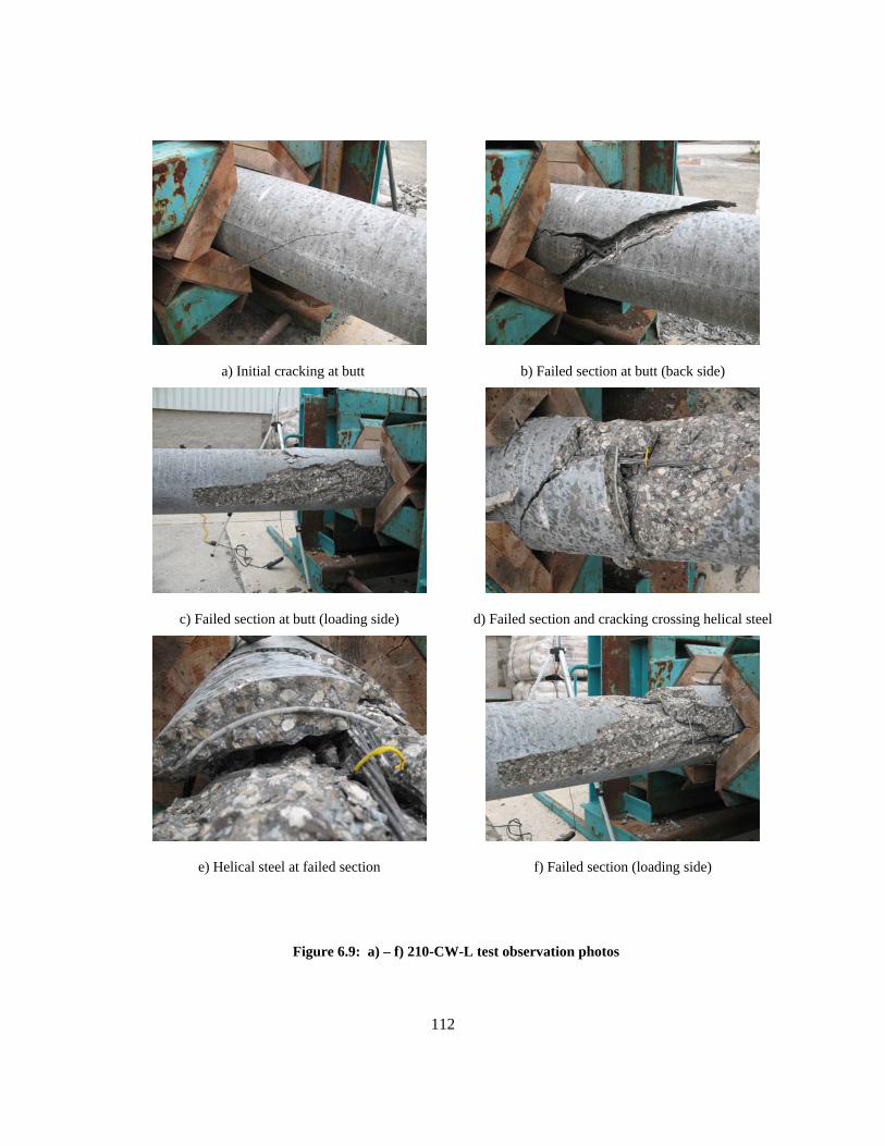
112


b) Failed section at butt (back side)

c) Failed section at butt (loading side)

d) Failed section and cracking crossing helical steel

e) Helical steel at failed section

f) Failed section (loading side)

Figure 6.9: a) – f) 210-CW-L test observation photos

113


b) Two sets of torsional cracks at butt

c) Failed section (back side)

d) Failed section (loading side)

e) Close up torsional cracks crossing failed helical steel

Figure 6.10: a) – e) 210-CCW-N test observation photos

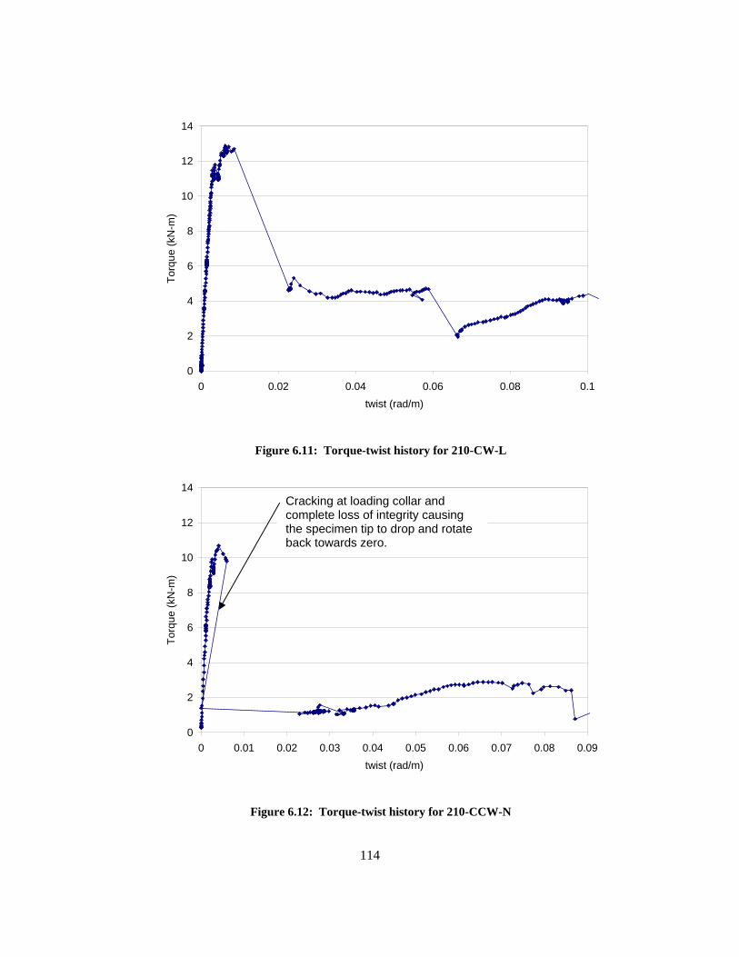
114

0

2

4

6

8

10

12

14

0 0.02 0.04 0.06 0.08 0.1twist (rad/m)

Torq

ue (k

N-m

)

Figure 6.11: Torque-twist history for 210-CW-L

0

2

4

6

8

10

12

14

0 0.01 0.02 0.03 0.04 0.05 0.06 0.07 0.08 0.09twist (rad/m)

Torq

ue (k

N-m

)

Figure 6.12: Torque-twist history for 210-CCW-N

Cracking at loading collar and complete loss of integrity causing the specimen tip to drop and rotate back towards zero.

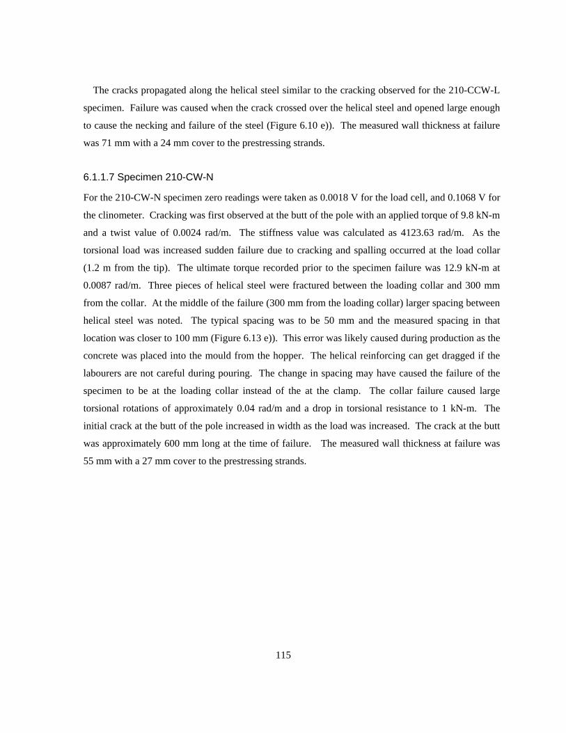
115

The cracks propagated along the helical steel similar to the cracking observed for the 210-CCW-L

specimen. Failure was caused when the crack crossed over the helical steel and opened large enough

to cause the necking and failure of the steel (Figure 6.10 e)). The measured wall thickness at failure

was 71 mm with a 24 mm cover to the prestressing strands.

6.1.1.7 Specimen 210-CW-N

For the 210-CW-N specimen zero readings were taken as 0.0018 V for the load cell, and 0.1068 V for

the clinometer. Cracking was first observed at the butt of the pole with an applied torque of 9.8 kN-m

and a twist value of 0.0024 rad/m. The stiffness value was calculated as 4123.63 rad/m. As the

torsional load was increased sudden failure due to cracking and spalling occurred at the load collar

(1.2 m from the tip). The ultimate torque recorded prior to the specimen failure was 12.9 kN-m at

0.0087 rad/m. Three pieces of helical steel were fractured between the loading collar and 300 mm

from the collar. At the middle of the failure (300 mm from the loading collar) larger spacing between

helical steel was noted. The typical spacing was to be 50 mm and the measured spacing in that

location was closer to 100 mm (Figure 6.13 e)). This error was likely caused during production as the

concrete was placed into the mould from the hopper. The helical reinforcing can get dragged if the

labourers are not careful during pouring. The change in spacing may have caused the failure of the

specimen to be at the loading collar instead of the at the clamp. The collar failure caused large

torsional rotations of approximately 0.04 rad/m and a drop in torsional resistance to 1 kN-m. The

initial crack at the butt of the pole increased in width as the load was increased. The crack at the butt

was approximately 600 mm long at the time of failure. The measured wall thickness at failure was

55 mm with a 27 mm cover to the prestressing strands.

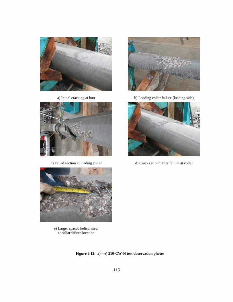
116


b) Loading collar failure (loading side)

c) Failed section at loading collar

d) Cracks at butt after failure at collar

e) Larger spaced helical steel at collar failure location

Figure 6.13: a) – e) 210-CW-N test observation photos

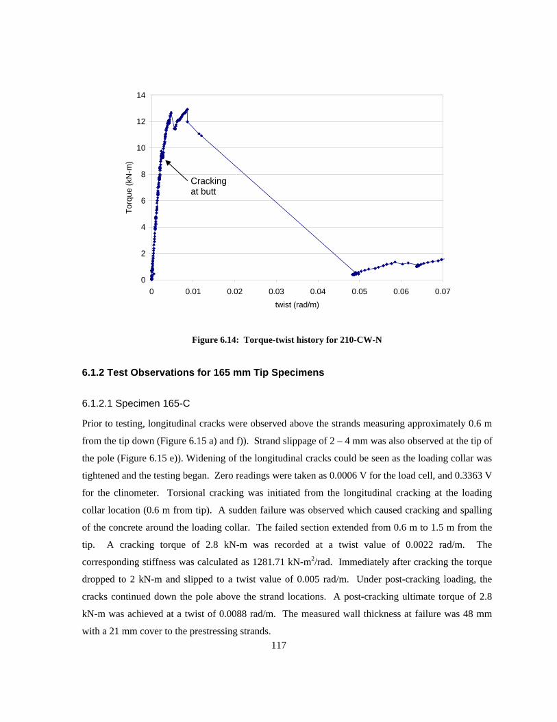
117

0

2

4

6

8

10

12

14

0 0.01 0.02 0.03 0.04 0.05 0.06 0.07twist (rad/m)

Torq

ue (k

N-m

)

Figure 6.14: Torque-twist history for 210-CW-N

6.1.2 Test Observations for 165 mm Tip Specimens

6.1.2.1 Specimen 165-C

Prior to testing, longitudinal cracks were observed above the strands measuring approximately 0.6 m

from the tip down (Figure 6.15 a) and f)). Strand slippage of 2 – 4 mm was also observed at the tip of

the pole (Figure 6.15 e)). Widening of the longitudinal cracks could be seen as the loading collar was

tightened and the testing began. Zero readings were taken as 0.0006 V for the load cell, and 0.3363 V

for the clinometer. Torsional cracking was initiated from the longitudinal cracking at the loading

collar location (0.6 m from tip). A sudden failure was observed which caused cracking and spalling

of the concrete around the loading collar. The failed section extended from 0.6 m to 1.5 m from the

tip. A cracking torque of 2.8 kN-m was recorded at a twist value of 0.0022 rad/m. The

corresponding stiffness was calculated as 1281.71 kN-m2/rad. Immediately after cracking the torque

dropped to 2 kN-m and slipped to a twist value of 0.005 rad/m. Under post-cracking loading, the

cracks continued down the pole above the strand locations. A post-cracking ultimate torque of 2.8

kN-m was achieved at a twist of 0.0088 rad/m. The measured wall thickness at failure was 48 mm

with a 21 mm cover to the prestressing strands.

Cracking at butt

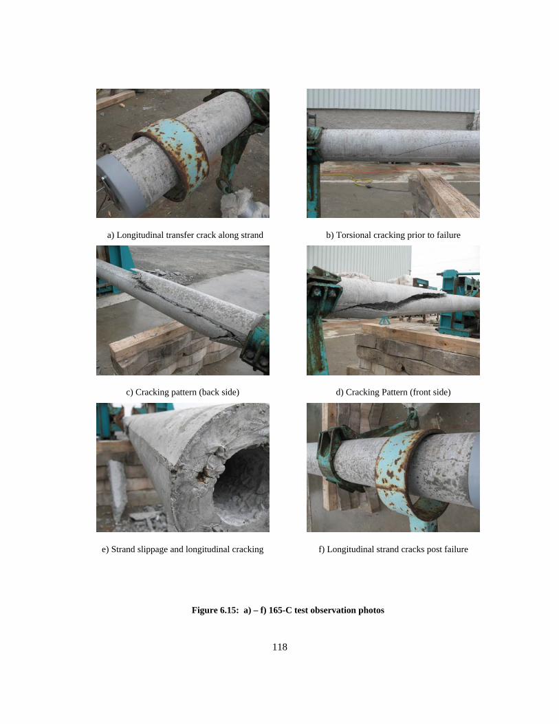
118

a) Longitudinal transfer crack along strand

b) Torsional cracking prior to failure

c) Cracking pattern (back side)

d) Cracking Pattern (front side)

e) Strand slippage and longitudinal cracking

f) Longitudinal strand cracks post failure

Figure 6.15: a) – f) 165-C test observation photos

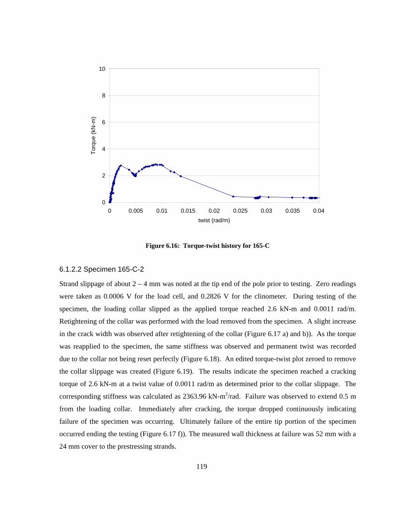
119

0

2

4

6

8

10

0 0.005 0.01 0.015 0.02 0.025 0.03 0.035 0.04twist (rad/m)

Torq

ue (k

N-m

)

Figure 6.16: Torque-twist history for 165-C

6.1.2.2 Specimen 165-C-2

Strand slippage of about 2 – 4 mm was noted at the tip end of the pole prior to testing. Zero readings

were taken as 0.0006 V for the load cell, and 0.2826 V for the clinometer. During testing of the

specimen, the loading collar slipped as the applied torque reached 2.6 kN-m and 0.0011 rad/m.

Retightening of the collar was performed with the load removed from the specimen. A slight increase

in the crack width was observed after retightening of the collar (Figure 6.17 a) and b)). As the torque

was reapplied to the specimen, the same stiffness was observed and permanent twist was recorded

due to the collar not being reset perfectly (Figure 6.18). An edited torque-twist plot zeroed to remove

the collar slippage was created (Figure 6.19). The results indicate the specimen reached a cracking

torque of 2.6 kN-m at a twist value of 0.0011 rad/m as determined prior to the collar slippage. The

corresponding stiffness was calculated as 2363.96 kN-m2/rad. Failure was observed to extend 0.5 m

from the loading collar. Immediately after cracking, the torque dropped continuously indicating

failure of the specimen was occurring. Ultimately failure of the entire tip portion of the specimen

occurred ending the testing (Figure 6.17 f)). The measured wall thickness at failure was 52 mm with a

24 mm cover to the prestressing strands.

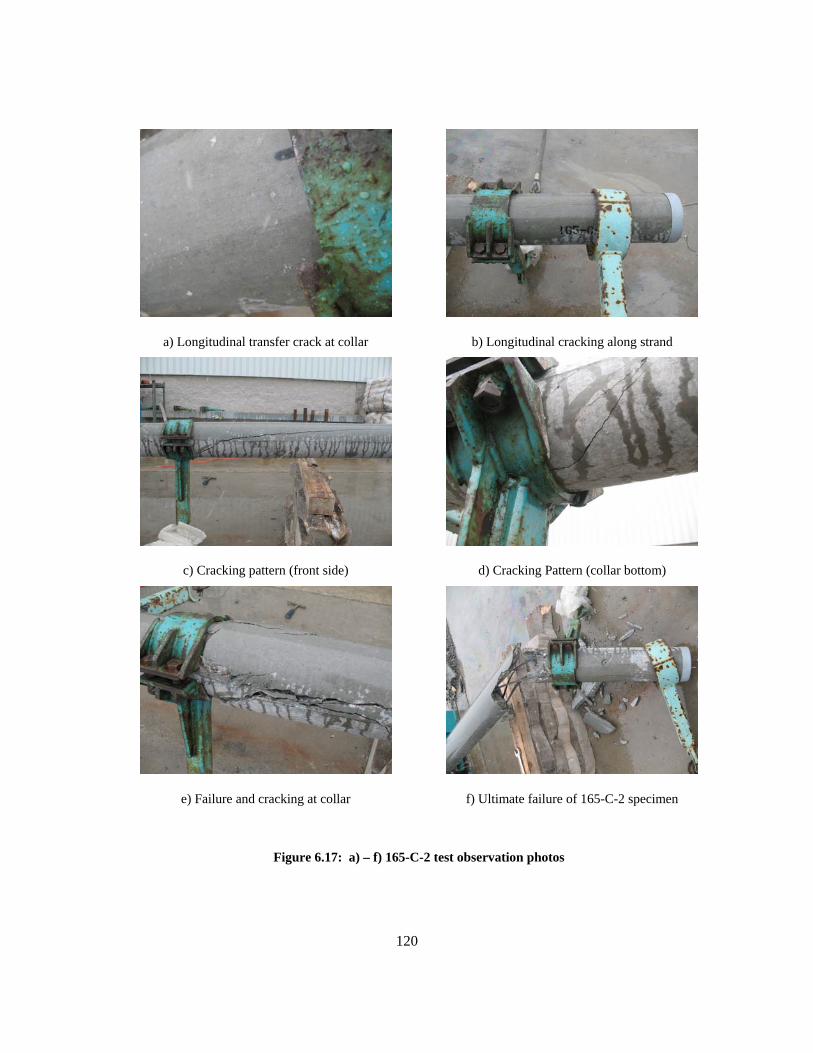
120

a) Longitudinal transfer crack at collar

b) Longitudinal cracking along strand

c) Cracking pattern (front side)

d) Cracking Pattern (collar bottom)

e) Failure and cracking at collar

f) Ultimate failure of 165-C-2 specimen

Figure 6.17: a) – f) 165-C-2 test observation photos

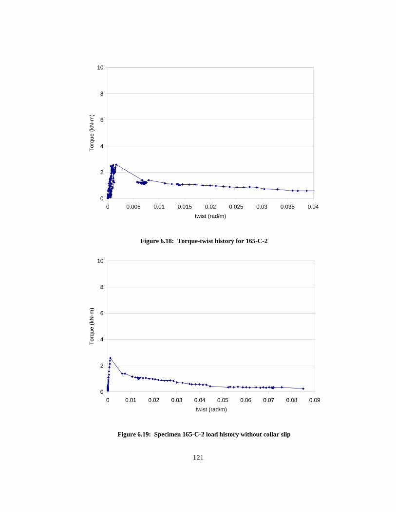
121

0

2

4

6

8

10

0 0.005 0.01 0.015 0.02 0.025 0.03 0.035 0.04twist (rad/m)

Torq

ue (k

N-m

)

Figure 6.18: Torque-twist history for 165-C-2

0

2

4

6

8

10

0 0.01 0.02 0.03 0.04 0.05 0.06 0.07 0.08 0.09twist (rad/m)

Torq

ue (k

N-m

)

Figure 6.19: Specimen 165-C-2 load history without collar slip

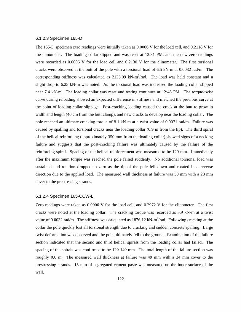
122

6.1.2.3 Specimen 165-D

The 165-D specimen zero readings were initially taken as 0.0006 V for the load cell, and 0.2118 V for

the clinometer. The loading collar slipped and was reset at 12:31 PM, and the new zero readings

were recorded as 0.0006 V for the load cell and 0.2130 V for the clinometer. The first torsional

cracks were observed at the butt of the pole with a torsional load of 6.5 kN-m at 0.0032 rad/m. The

corresponding stiffness was calculated as 2123.09 kN-m2/rad. The load was held constant and a

slight drop to 6.25 kN-m was noted. As the torsional load was increased the loading collar slipped

near 7.4 kN-m. The loading collar was reset and testing continues at 12:48 PM. The torque-twist

curve during reloading showed an expected difference in stiffness and matched the previous curve at

the point of loading collar slippage. Post-cracking loading caused the crack at the butt to grow in

width and length (40 cm from the butt clamp), and new cracks to develop near the loading collar. The

pole reached an ultimate cracking torque of 8.1 kN-m at a twist value of 0.0071 rad/m. Failure was

caused by spalling and torsional cracks near the loading collar (0.9 m from the tip). The third spiral

of the helical reinforcing (approximately 350 mm from the loading collar) showed signs of a necking

failure and suggests that the post-cracking failure was ultimately caused by the failure of the

reinforcing spiral. Spacing of the helical reinforcement was measured to be 120 mm. Immediately

after the maximum torque was reached the pole failed suddenly. No additional torsional load was

sustained and rotation dropped to zero as the tip of the pole fell down and rotated in a reverse

direction due to the applied load. The measured wall thickness at failure was 50 mm with a 28 mm

cover to the prestressing strands.

6.1.2.4 Specimen 165-CCW-L

Zero readings were taken as 0.0006 V for the load cell, and 0.2972 V for the clinometer. The first

cracks were noted at the loading collar. The cracking torque was recorded as 5.9 kN-m at a twist

value of 0.0032 rad/m. The stiffness was calculated as 1876.12 kN-m2/rad. Following cracking at the

collar the pole quickly lost all torsional strength due to cracking and sudden concrete spalling. Large

twist deformation was observed and the pole ultimately fell to the ground. Examination of the failure

section indicated that the second and third helical spirals from the loading collar had failed. The

spacing of the spirals was confirmed to be 120-140 mm. The total length of the failure section was

roughly 0.6 m. The measured wall thickness at failure was 49 mm with a 24 mm cover to the

prestressing strands. 15 mm of segregated cement paste was measured on the inner surface of the

wall.

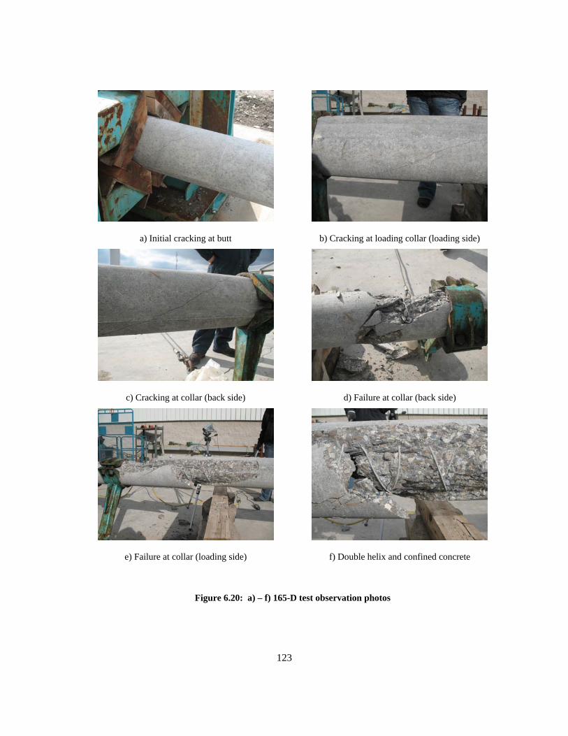
123


b) Cracking at loading collar (loading side)

c) Cracking at collar (back side)

d) Failure at collar (back side)

e) Failure at collar (loading side)

f) Double helix and confined concrete

Figure 6.20: a) – f) 165-D test observation photos

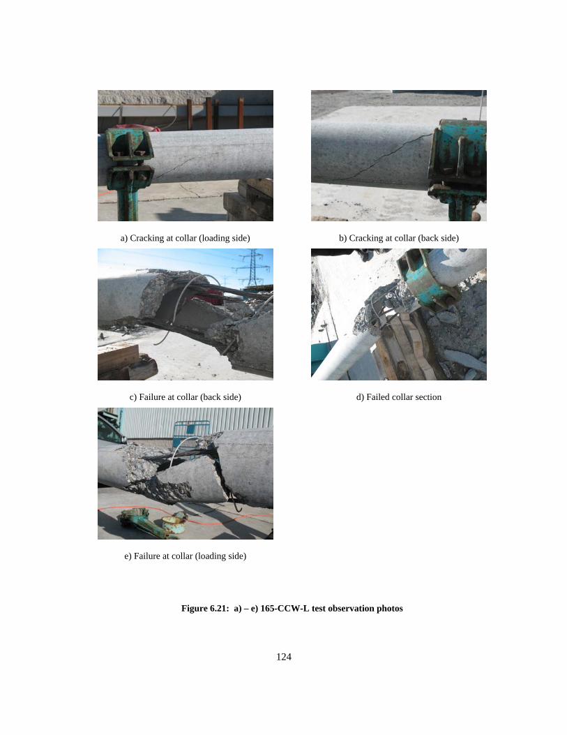
124

a) Cracking at collar (loading side)

b) Cracking at collar (back side)

c) Failure at collar (back side)

d) Failed collar section

e) Failure at collar (loading side)

Figure 6.21: a) – e) 165-CCW-L test observation photos

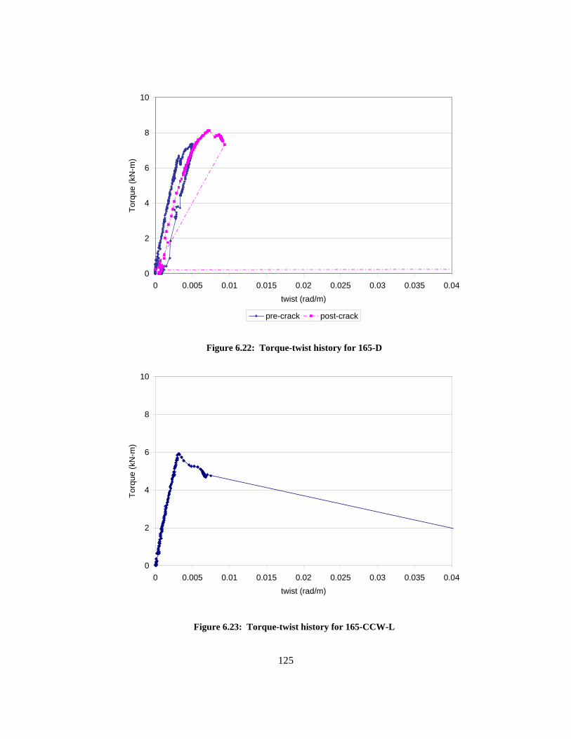
125

0

2

4

6

8

10

0 0.005 0.01 0.015 0.02 0.025 0.03 0.035 0.04twist (rad/m)

Torq

ue (k

N-m

)

pre-crack post-crack

Figure 6.22: Torque-twist history for 165-D

0

2

4

6

8

10

0 0.005 0.01 0.015 0.02 0.025 0.03 0.035 0.04twist (rad/m)

Torq

ue (k

N-m

)

Figure 6.23: Torque-twist history for 165-CCW-L

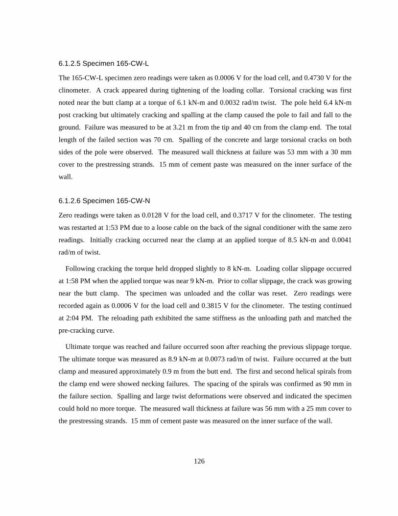
126

6.1.2.5 Specimen 165-CW-L

The 165-CW-L specimen zero readings were taken as 0.0006 V for the load cell, and 0.4730 V for the

clinometer. A crack appeared during tightening of the loading collar. Torsional cracking was first

noted near the butt clamp at a torque of 6.1 kN-m and 0.0032 rad/m twist. The pole held 6.4 kN-m

post cracking but ultimately cracking and spalling at the clamp caused the pole to fail and fall to the

ground. Failure was measured to be at 3.21 m from the tip and 40 cm from the clamp end. The total

length of the failed section was 70 cm. Spalling of the concrete and large torsional cracks on both

sides of the pole were observed. The measured wall thickness at failure was 53 mm with a 30 mm

cover to the prestressing strands. 15 mm of cement paste was measured on the inner surface of the

wall.

6.1.2.6 Specimen 165-CW-N

Zero readings were taken as 0.0128 V for the load cell, and 0.3717 V for the clinometer. The testing

was restarted at 1:53 PM due to a loose cable on the back of the signal conditioner with the same zero

readings. Initially cracking occurred near the clamp at an applied torque of 8.5 kN-m and 0.0041

rad/m of twist.

Following cracking the torque held dropped slightly to 8 kN-m. Loading collar slippage occurred

at 1:58 PM when the applied torque was near 9 kN-m. Prior to collar slippage, the crack was growing

near the butt clamp. The specimen was unloaded and the collar was reset. Zero readings were

recorded again as 0.0006 V for the load cell and 0.3815 V for the clinometer. The testing continued

at 2:04 PM. The reloading path exhibited the same stiffness as the unloading path and matched the

pre-cracking curve.

Ultimate torque was reached and failure occurred soon after reaching the previous slippage torque.

The ultimate torque was measured as 8.9 kN-m at 0.0073 rad/m of twist. Failure occurred at the butt

clamp and measured approximately 0.9 m from the butt end. The first and second helical spirals from

the clamp end were showed necking failures. The spacing of the spirals was confirmed as 90 mm in

the failure section. Spalling and large twist deformations were observed and indicated the specimen

could hold no more torque. The measured wall thickness at failure was 56 mm with a 25 mm cover to

the prestressing strands. 15 mm of cement paste was measured on the inner surface of the wall.

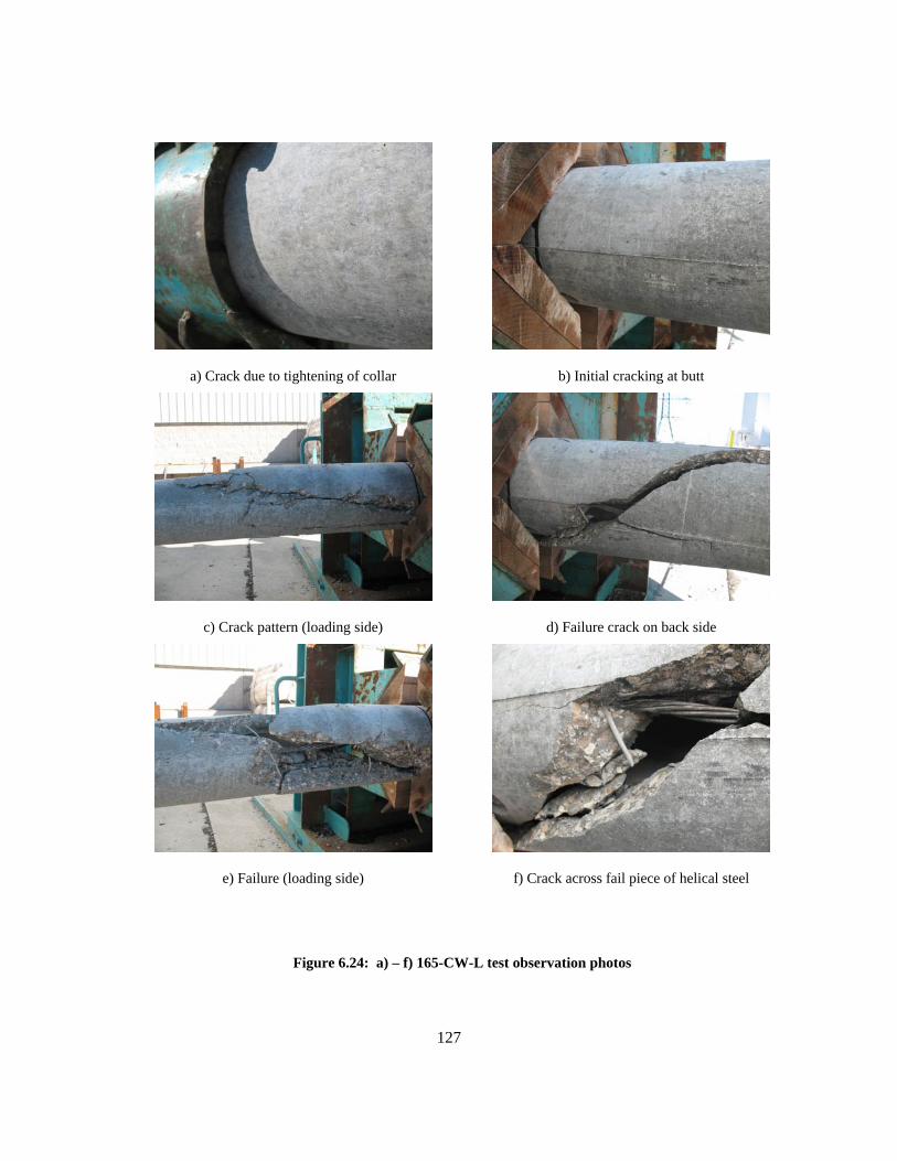
127

a) Crack due to tightening of collar

b) Initial cracking at butt

c) Crack pattern (loading side)

d) Failure crack on back side

e) Failure (loading side)

f) Crack across fail piece of helical steel

Figure 6.24: a) – f) 165-CW-L test observation photos

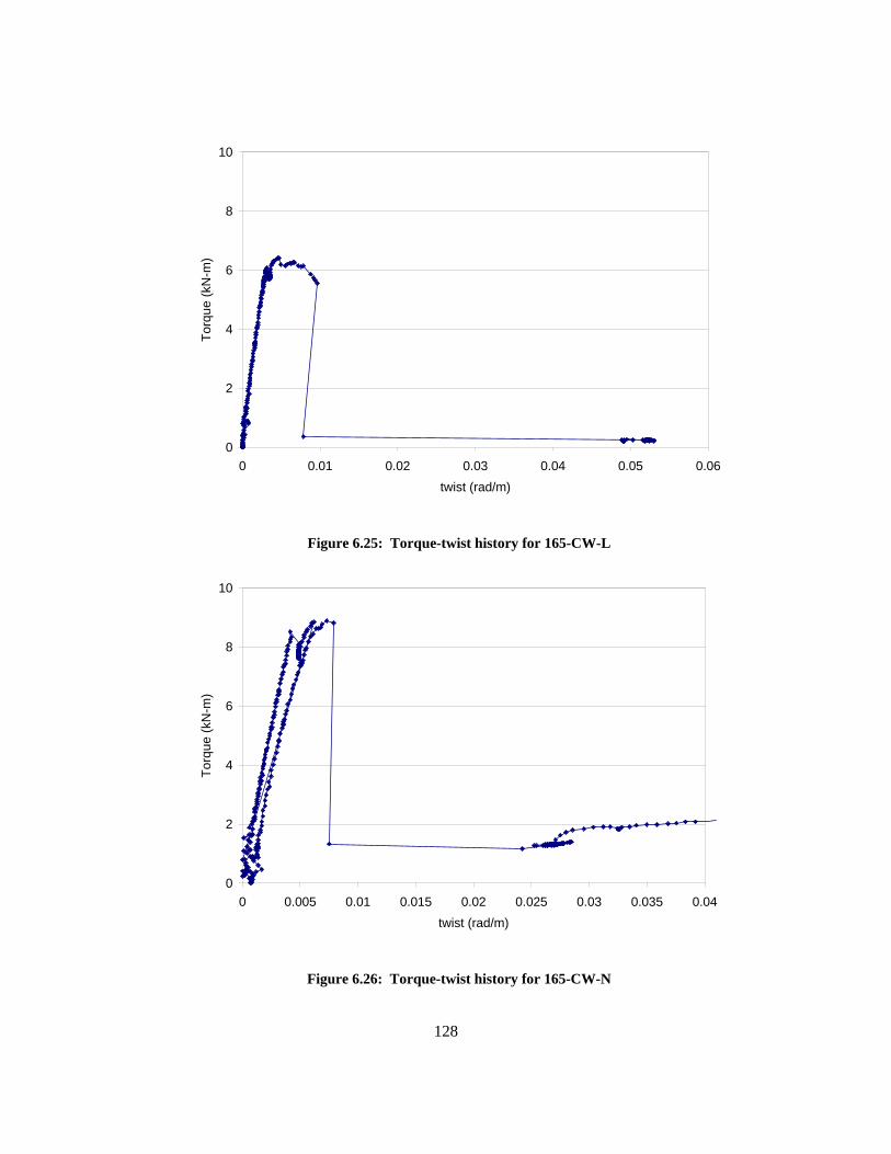
128

0

2

4

6

8

10

0 0.01 0.02 0.03 0.04 0.05 0.06twist (rad/m)

Torq

ue (k

N-m

)

Figure 6.25: Torque-twist history for 165-CW-L

0

2

4

6

8

10

0 0.005 0.01 0.015 0.02 0.025 0.03 0.035 0.04twist (rad/m)

Torq

ue (k

N-m

)

Figure 6.26: Torque-twist history for 165-CW-N

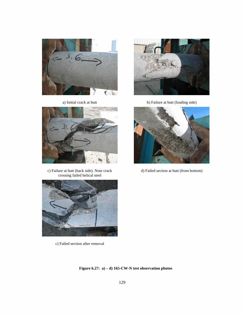
129

a) Initial crack at butt

b) Failure at butt (loading side)

c) Failure at butt (back side). Note crack crossing failed helical steel

d) Failed section at butt (from bottom)

c) Failed section after removal

Figure 6.27: a) – d) 165-CW-N test observation photos

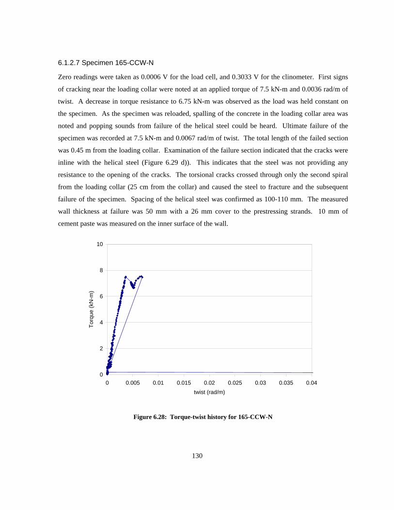
130

6.1.2.7 Specimen 165-CCW-N

Zero readings were taken as 0.0006 V for the load cell, and 0.3033 V for the clinometer. First signs

of cracking near the loading collar were noted at an applied torque of 7.5 kN-m and 0.0036 rad/m of

twist. A decrease in torque resistance to 6.75 kN-m was observed as the load was held constant on

the specimen. As the specimen was reloaded, spalling of the concrete in the loading collar area was

noted and popping sounds from failure of the helical steel could be heard. Ultimate failure of the

specimen was recorded at 7.5 kN-m and 0.0067 rad/m of twist. The total length of the failed section

was 0.45 m from the loading collar. Examination of the failure section indicated that the cracks were

inline with the helical steel (Figure 6.29 d)). This indicates that the steel was not providing any

resistance to the opening of the cracks. The torsional cracks crossed through only the second spiral

from the loading collar (25 cm from the collar) and caused the steel to fracture and the subsequent

failure of the specimen. Spacing of the helical steel was confirmed as 100-110 mm. The measured

wall thickness at failure was 50 mm with a 26 mm cover to the prestressing strands. 10 mm of

cement paste was measured on the inner surface of the wall.

0

2

4

6

8

10

0 0.005 0.01 0.015 0.02 0.025 0.03 0.035 0.04twist (rad/m)

Torq

ue (k

N-m

)

Figure 6.28: Torque-twist history for 165-CCW-N

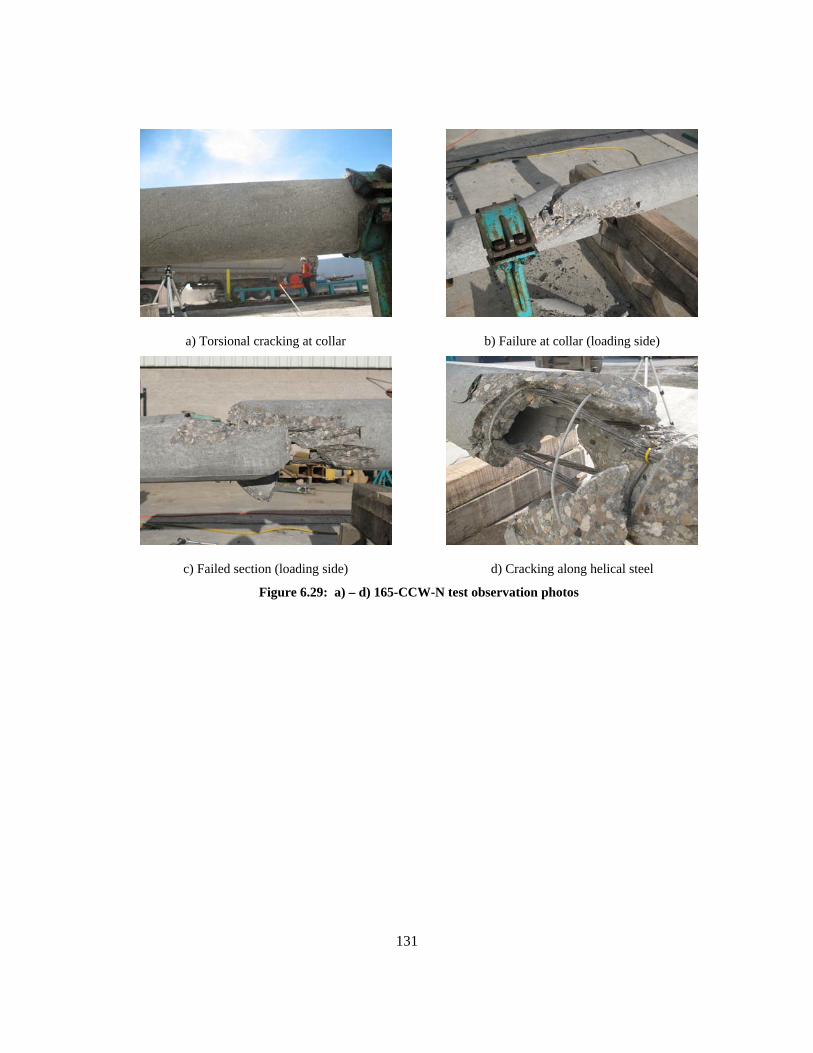
131

a) Torsional cracking at collar

b) Failure at collar (loading side)

c) Failed section (loading side)

d) Cracking along helical steel

Figure 6.29: a) – d) 165-CCW-N test observation photos

132

Chapter 7 Analysis of Experimental Results

7.1 General Experimental Results

This chapter contains the analysis of the results, which are used to determine the influence that helical

reinforcing spacing, direction, wall thickness, and other factors have on the cracking torque of

prestressed concrete poles. The results are also compared to two torsion models (presented in section

2.6) and analyzed to determine how well the models can predict the experimental results. Cracking

torque formulae are presented and compared to the experimental data to establish whether the torsion

capacity of concrete poles can be accurately calculated. The variation in the experimental results is

analyzed and the potential causes for the variations discussed. Finally, strut and tie models are used

to determine the required spacing of the helical reinforcing in the prestressing transfer zone and

minimum transverse reinforcement requirements from the concrete codes and literature will be

discussed.

The data collected during the testing allowed the entire torque-twist history of each pole to be

plotted (Figure 7.1 and Figure 7.2). All experimental data figures present the torque and twist

response of the pole specimens at 0.6 m from the tip. The torque is given in kN-m and the twist in

rad/m. The twist angle measured was divided by the length of each specimen to account for slight

variations in the tested length of the specimens. All CCW labelled specimens were tested in the

counter clockwise direction indicating that the helical steel was theoretically ineffective (see Section

4.2). The CW specimens were tested in the clockwise direction and had effective helical steel.

In general, the larger 210 mm specimens sustained an additional amount of torque after cracking.

The post-cracking additional load was in the range of 0.3 kN-m for the 165 mm tip poles and 2.4 kN-

m for the 210 mm tip poles. Failure in all cases was sudden and coincided with substantial rotation.

The load sustained after maximum torque had been achieved was less than half of the maximum

torque. The lower results of the CCW-L specimens may have been skewed due to the higher air

content and lower concrete strengths.

Figure 7.1 displays the 165 mm specimens. It should be noted that since all except for two of the

failures (165-CW-N and 165-CW-L) occurred at the loading collar. The torque-twist curves all

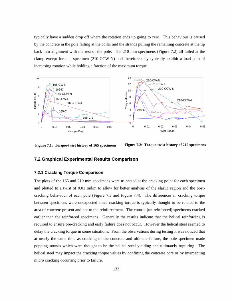
133

typically have a sudden drop off where the rotation ends up going to zero. This behaviour is caused

by the concrete in the pole failing at the collar and the strands pulling the remaining concrete at the tip

back into alignment with the rest of the pole. The 210 mm specimens (Figure 7.2) all failed at the

clamp except for one specimen (210-CCW-N) and therefore they typically exhibit a load path of

increasing rotation while holding a fraction of the maximum torque.

0

2

4

6

8

10

0 0.01 0.02 0.03 0.04 0.05twist (rad/m)

Torq

ue (k

N-m

)

165-C

165-C-2

165-CCW-L165-CW-L

165-D165-CW-N

165-CCW-N

Figure 7.1: Torque-twist history of 165 specimens

0

2

4

6

8

10

12

14

0 0.01 0.02 0.03 0.04 0.05twist (rad/m)

Torq

ue (k

N-m

)

210-C 210-C-2

210-CCW-L

210-CW-L210-D 210-CW-N

210-CCW-N

Figure 7.2: Torque-twist history of 210 specimens

7.2 Graphical Experimental Results Comparison

7.2.1 Cracking Torque Comparison

The plots of the 165 and 210 mm specimens were truncated at the cracking point for each specimen

and plotted to a twist of 0.01 rad/m to allow for better analysis of the elastic region and the post-

cracking behaviour of each pole (Figure 7.3 and Figure 7.4). The differences in cracking torque

between specimens were unexpected since cracking torque is typically thought to be related to the

area of concrete present and not to the reinforcement. The control (un-reinforced) specimens cracked

earlier than the reinforced specimens. Generally the results indicate that the helical reinforcing is

required to ensure pre-cracking and early failure does not occur. However the helical steel seemed to

delay the cracking torque in some situations. From the observations during testing it was noticed that

at nearly the same time as cracking of the concrete and ultimate failure, the pole specimen made

popping sounds which were thought to be the helical steel yielding and ultimately rupturing. The

helical steel may impact the cracking torque values by confining the concrete core or by intercepting

micro cracking occurring prior to failure.

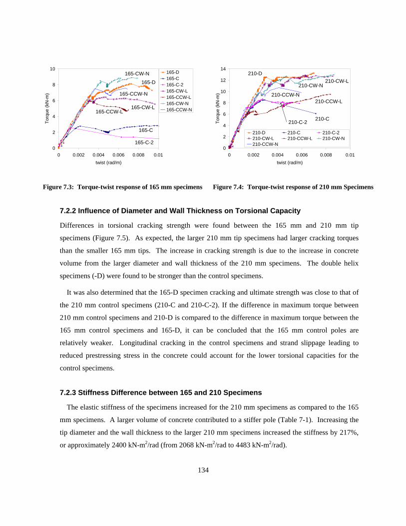
134

0

2

4

6

8

10

0 0.002 0.004 0.006 0.008 0.01twist (rad/m)

Torq

ue (k

N-m

)

165-D165-C165-C-2165-CW-L165-CCW-L165-CW-N165-CCW-N

165-C

165-C-2

165-CW-N

165-CCW-L165-CW-L

165-CCW-N

165-D

Figure 7.3: Torque-twist response of 165 mm specimens

0

2

4

6

8

10

12

14

0 0.002 0.004 0.006 0.008 0.01twist (rad/m)

Torq

ue (k

N-m

)

210-D 210-C 210-C-2210-CW-L 210-CCW-L 210-CW-N210-CCW-N

210-CCW-L

210-D

210-CW-N210-CW-L

210-CCW-N

210-C210-C-2

Figure 7.4: Torque-twist response of 210 mm Specimens

7.2.2 Influence of Diameter and Wall Thickness on Torsional Capacity

Differences in torsional cracking strength were found between the 165 mm and 210 mm tip

specimens (Figure 7.5). As expected, the larger 210 mm tip specimens had larger cracking torques

than the smaller 165 mm tips. The increase in cracking strength is due to the increase in concrete

volume from the larger diameter and wall thickness of the 210 mm specimens. The double helix

specimens (-D) were found to be stronger than the control specimens.

It was also determined that the 165-D specimen cracking and ultimate strength was close to that of

the 210 mm control specimens (210-C and 210-C-2). If the difference in maximum torque between

210 mm control specimens and 210-D is compared to the difference in maximum torque between the

165 mm control specimens and 165-D, it can be concluded that the 165 mm control poles are

relatively weaker. Longitudinal cracking in the control specimens and strand slippage leading to

reduced prestressing stress in the concrete could account for the lower torsional capacities for the

control specimens.

7.2.3 Stiffness Difference between 165 and 210 Specimens

The elastic stiffness of the specimens increased for the 210 mm specimens as compared to the 165

mm specimens. A larger volume of concrete contributed to a stiffer pole (Table 7-1). Increasing the

tip diameter and the wall thickness to the larger 210 mm specimens increased the stiffness by 217%,

or approximately 2400 kN-m2/rad (from 2068 kN-m2/rad to 4483 kN-m2/rad).

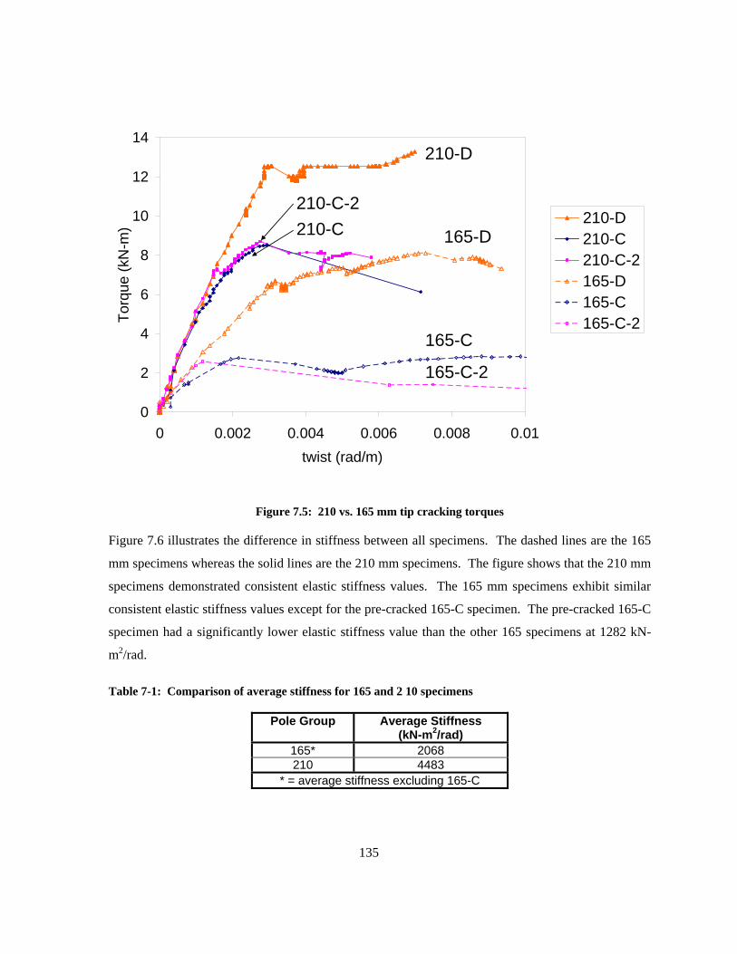
135

0

2

4

6

8

10

12

14

0 0.002 0.004 0.006 0.008 0.01twist (rad/m)

Torq

ue (k

N-m

) 210-D210-C210-C-2165-D165-C165-C-2

210-D

165-D

210-C-2210-C

165-C

165-C-2

Figure 7.5: 210 vs. 165 mm tip cracking torques

Figure 7.6 illustrates the difference in stiffness between all specimens. The dashed lines are the 165

mm specimens whereas the solid lines are the 210 mm specimens. The figure shows that the 210 mm

specimens demonstrated consistent elastic stiffness values. The 165 mm specimens exhibit similar

consistent elastic stiffness values except for the pre-cracked 165-C specimen. The pre-cracked 165-C

specimen had a significantly lower elastic stiffness value than the other 165 specimens at 1282 kN-

m2/rad.

Table 7-1: Comparison of average stiffness for 165 and 2 10 specimens

Pole Group Average Stiffness (kN-m2/rad)

165* 2068 210 4483

* = average stiffness excluding 165-C

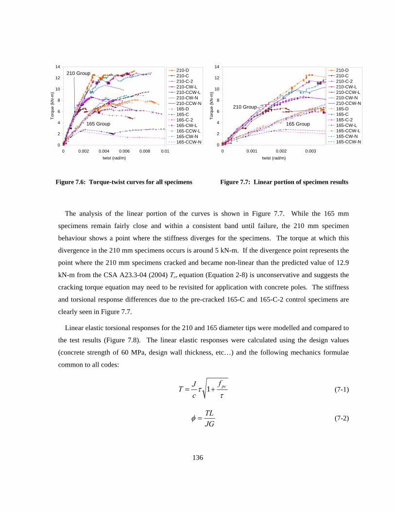
136

0

2

4

6

8

10

12

14

0 0.002 0.004 0.006 0.008 0.01twist (rad/m)

Torq

ue (k

N-m

)

210-D210-C210-C-2210-CW-L210-CCW-L210-CW-N210-CCW-N165-D165-C165-C-2165-CW-L165-CCW-L165-CW-N165-CCW-N

210 Group

165 Group

Figure 7.6: Torque-twist curves for all specimens

0

2

4

6

8

10

12

14

0 0.001 0.002 0.003twist (rad/m)

Torq

ue (k

N-m

)

210-D210-C210-C-2210-CW-L210-CCW-L210-CW-N210-CCW-N165-D165-C165-C-2165-CW-L165-CCW-L165-CW-N165-CCW-N

210 Group

165 Group

Figure 7.7: Linear portion of specimen results

The analysis of the linear portion of the curves is shown in Figure 7.7. While the 165 mm

specimens remain fairly close and within a consistent band until failure, the 210 mm specimen

behaviour shows a point where the stiffness diverges for the specimens. The torque at which this

divergence in the 210 mm specimens occurs is around 5 kN-m. If the divergence point represents the

point where the 210 mm specimens cracked and became non-linear than the predicted value of 12.9

kN-m from the CSA A23.3-04 (2004) Tcr equation (Equation 2-8) is unconservative and suggests the

cracking torque equation may need to be revisited for application with concrete poles. The stiffness

and torsional response differences due to the pre-cracked 165-C and 165-C-2 control specimens are

clearly seen in Figure 7.7.

Linear elastic torsional responses for the 210 and 165 diameter tips were modelled and compared to

the test results (Figure 7.8). The linear elastic responses were calculated using the design values

(concrete strength of 60 MPa, design wall thickness, etc…) and the following mechanics formulae

common to all codes:

τ

τ pcfcJT += 1 (7-1)

JGTL

=φ (7-2)

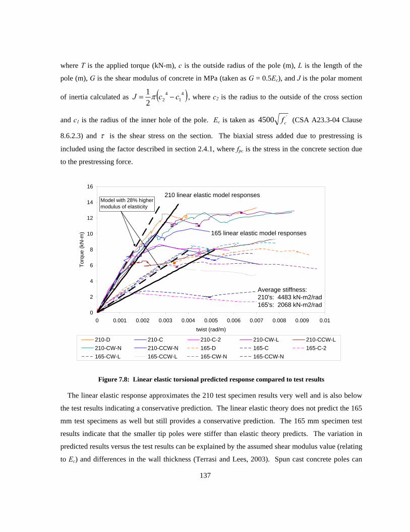
137

where T is the applied torque (kN-m), c is the outside radius of the pole (m), L is the length of the

pole (m), G is the shear modulus of concrete in MPa (taken as G = 0.5Ec), and J is the polar moment

of inertia calculated as ( )41

422

1 ccJ −= π , where c2 is the radius to the outside of the cross section

and c1 is the radius of the inner hole of the pole. Ec is taken as `4500 cf (CSA A23.3-04 Clause

8.6.2.3) and τ is the shear stress on the section. The biaxial stress added due to prestressing is

included using the factor described in section 2.4.1, where fpc is the stress in the concrete section due

to the prestressing force.

0

2

4

6

8

10

12

14

16

0 0.001 0.002 0.003 0.004 0.005 0.006 0.007 0.008 0.009 0.01twist (rad/m)

Torq

ue (k

N-m

)

210-D 210-C 210-C-2 210-CW-L 210-CCW-L210-CW-N 210-CCW-N 165-D 165-C 165-C-2165-CW-L 165-CCW-L 165-CW-N 165-CCW-N

210 linear elastic model responses

165 linear elastic model responses

Average stiffness:210's: 4483 kN-m2/rad165's: 2068 kN-m2/rad

Model with 28% higher modulus of elasticity

Figure 7.8: Linear elastic torsional predicted response compared to test results

The linear elastic response approximates the 210 test specimen results very well and is also below

the test results indicating a conservative prediction. The linear elastic theory does not predict the 165

mm test specimens as well but still provides a conservative prediction. The 165 mm specimen test

results indicate that the smaller tip poles were stiffer than elastic theory predicts. The variation in

predicted results versus the test results can be explained by the assumed shear modulus value (relating

to Ec) and differences in the wall thickness (Terrasi and Lees, 2003). Spun cast concrete poles can

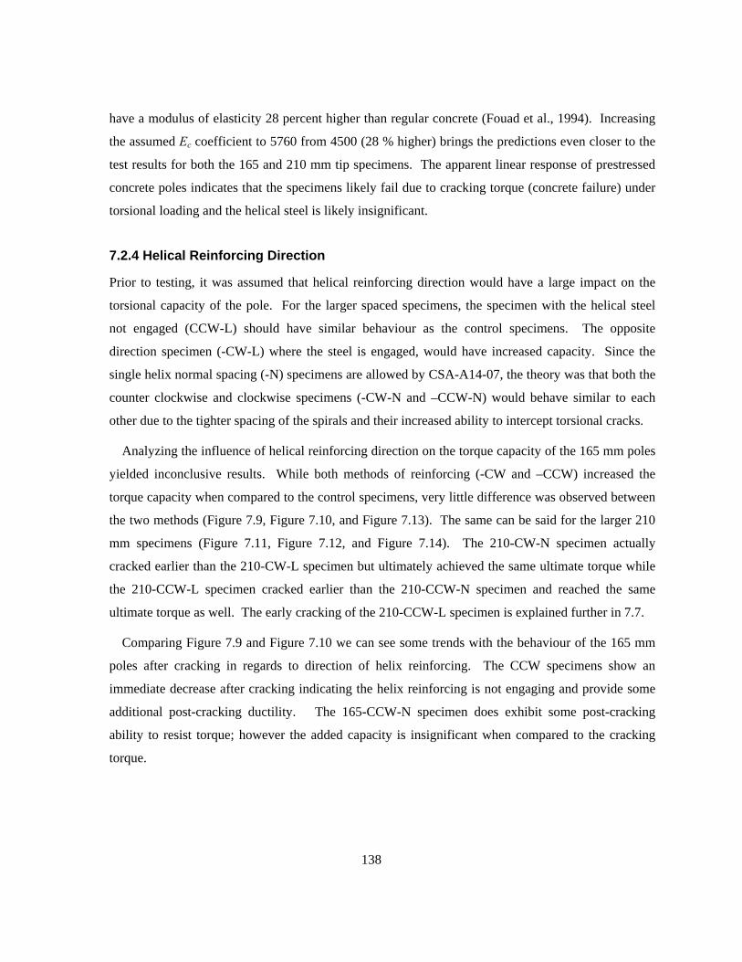
138

have a modulus of elasticity 28 percent higher than regular concrete (Fouad et al., 1994). Increasing

the assumed Ec coefficient to 5760 from 4500 (28 % higher) brings the predictions even closer to the

test results for both the 165 and 210 mm tip specimens. The apparent linear response of prestressed

concrete poles indicates that the specimens likely fail due to cracking torque (concrete failure) under

torsional loading and the helical steel is likely insignificant.

7.2.4 Helical Reinforcing Direction

Prior to testing, it was assumed that helical reinforcing direction would have a large impact on the

torsional capacity of the pole. For the larger spaced specimens, the specimen with the helical steel

not engaged (CCW-L) should have similar behaviour as the control specimens. The opposite

direction specimen (-CW-L) where the steel is engaged, would have increased capacity. Since the

single helix normal spacing (-N) specimens are allowed by CSA-A14-07, the theory was that both the

counter clockwise and clockwise specimens (-CW-N and –CCW-N) would behave similar to each

other due to the tighter spacing of the spirals and their increased ability to intercept torsional cracks.

Analyzing the influence of helical reinforcing direction on the torque capacity of the 165 mm poles

yielded inconclusive results. While both methods of reinforcing (-CW and –CCW) increased the

torque capacity when compared to the control specimens, very little difference was observed between

the two methods (Figure 7.9, Figure 7.10, and Figure 7.13). The same can be said for the larger 210

mm specimens (Figure 7.11, Figure 7.12, and Figure 7.14). The 210-CW-N specimen actually

cracked earlier than the 210-CW-L specimen but ultimately achieved the same ultimate torque while

the 210-CCW-L specimen cracked earlier than the 210-CCW-N specimen and reached the same

ultimate torque as well. The early cracking of the 210-CCW-L specimen is explained further in 7.7.

Comparing Figure 7.9 and Figure 7.10 we can see some trends with the behaviour of the 165 mm

poles after cracking in regards to direction of helix reinforcing. The CCW specimens show an

immediate decrease after cracking indicating the helix reinforcing is not engaging and provide some

additional post-cracking ductility. The 165-CCW-N specimen does exhibit some post-cracking

ability to resist torque; however the added capacity is insignificant when compared to the cracking

torque.

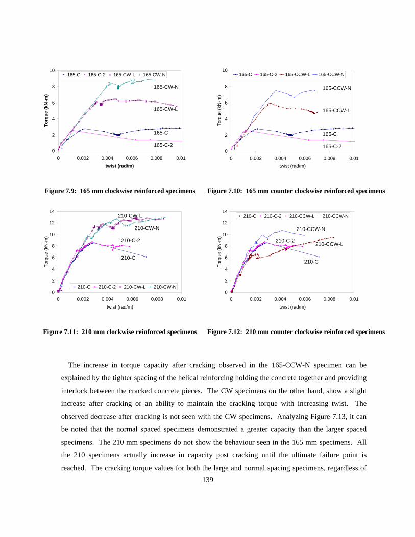
139

0

2

4

6

8

10

0 0.002 0.004 0.006 0.008 0.01twist (rad/m)

Torq

ue (k

N-m

)

165-C 165-C-2 165-CW-L 165-CW-N

165-C

165-C-2

165-CW-L

165-CW-N

Figure 7.9: 165 mm clockwise reinforced specimens

0

2

4

6

8

10

0 0.002 0.004 0.006 0.008 0.01twist (rad/m)

Torq

ue (k

N-m

)

165-C 165-C-2 165-CCW-L 165-CCW-N

165-C

165-C-2

165-CCW-L

165-CCW-N

Figure 7.10: 165 mm counter clockwise reinforced specimens

0

2

4

6

8

10

12

14

0 0.002 0.004 0.006 0.008 0.01twist (rad/m)

Torq

ue (k

N-m

)

210-C 210-C-2 210-CW-L 210-CW-N

210-C

210-C-2

210-CW-L

210-CW-N

Figure 7.11: 210 mm clockwise reinforced specimens

0

2

4

6

8

10

12

14

0 0.002 0.004 0.006 0.008 0.01twist (rad/m)

Torq

ue (k

N-m

)210-C 210-C-2 210-CCW-L 210-CCW-N

210-C

210-C-2

210-CCW-N

210-CCW-L

Figure 7.12: 210 mm counter clockwise reinforced specimens

The increase in torque capacity after cracking observed in the 165-CCW-N specimen can be

explained by the tighter spacing of the helical reinforcing holding the concrete together and providing

interlock between the cracked concrete pieces. The CW specimens on the other hand, show a slight

increase after cracking or an ability to maintain the cracking torque with increasing twist. The

observed decrease after cracking is not seen with the CW specimens. Analyzing Figure 7.13, it can

be noted that the normal spaced specimens demonstrated a greater capacity than the larger spaced

specimens. The 210 mm specimens do not show the behaviour seen in the 165 mm specimens. All

the 210 specimens actually increase in capacity post cracking until the ultimate failure point is

reached. The cracking torque values for both the large and normal spacing specimens, regardless of

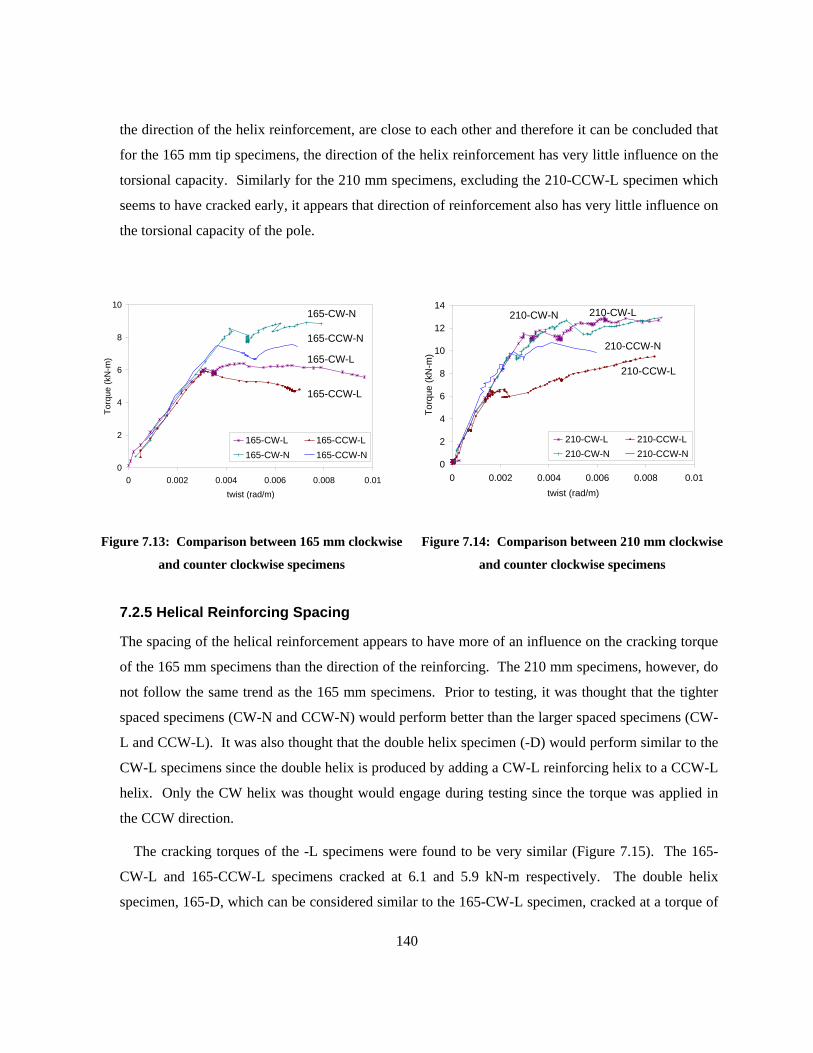
140

the direction of the helix reinforcement, are close to each other and therefore it can be concluded that

for the 165 mm tip specimens, the direction of the helix reinforcement has very little influence on the

torsional capacity. Similarly for the 210 mm specimens, excluding the 210-CCW-L specimen which

seems to have cracked early, it appears that direction of reinforcement also has very little influence on

the torsional capacity of the pole.

0

2

4

6

8

10

0 0.002 0.004 0.006 0.008 0.01twist (rad/m)

Torq

ue (k

N-m

)

165-CW-L 165-CCW-L165-CW-N 165-CCW-N

165-CW-L

165-CW-N

165-CCW-L

165-CCW-N

Figure 7.13: Comparison between 165 mm clockwise

and counter clockwise specimens

0

2

4

6

8

10

12

14

0 0.002 0.004 0.006 0.008 0.01twist (rad/m)

Torq

ue (k

N-m

)210-CW-L 210-CCW-L210-CW-N 210-CCW-N

210-CCW-N

210-CW-L210-CW-N

210-CCW-L

Figure 7.14: Comparison between 210 mm clockwise

and counter clockwise specimens

7.2.5 Helical Reinforcing Spacing

The spacing of the helical reinforcement appears to have more of an influence on the cracking torque

of the 165 mm specimens than the direction of the reinforcing. The 210 mm specimens, however, do

not follow the same trend as the 165 mm specimens. Prior to testing, it was thought that the tighter

spaced specimens (CW-N and CCW-N) would perform better than the larger spaced specimens (CW-

L and CCW-L). It was also thought that the double helix specimen (-D) would perform similar to the

CW-L specimens since the double helix is produced by adding a CW-L reinforcing helix to a CCW-L

helix. Only the CW helix was thought would engage during testing since the torque was applied in

the CCW direction.

The cracking torques of the -L specimens were found to be very similar (Figure 7.15). The 165-

CW-L and 165-CCW-L specimens cracked at 6.1 and 5.9 kN-m respectively. The double helix

specimen, 165-D, which can be considered similar to the 165-CW-L specimen, cracked at a torque of

141

6.7 kN-m. While the cracking torques of each specimen was similar, the behaviour after cracking

differed. The 165-D specimen was able to hold additional post-cracking torque, increasing to 8.1 kN-

m. The large spaced specimens on the other hand held no additional load (165-CCW-L) or

maintained approximately the cracking torque value while the twist continued to increase (165-CW-

L). The increase in torque after cracking observed for the 165-D specimen is likely caused by the

increased ratio of helical reinforcement. Since the 165-D specimen contained the same volume of

helical steel as the normal spaced specimens, an increase in ultimate torsional capacity for the double

helix specimen is expected when compared to the large spaced specimens.

The results of the 165 mm pole testing suggest that the normal spaced specimens have higher

cracking torque values than the larger spaced specimens. Respectively the 165-CW-N and 165-

CCW-N specimens cracked at 8.5 and 7.5 kN-m (Figure 7.16). Both normal spaced specimen

showed very little ability to hold additional load after cracking and held about the same torque as the

165-D specimen after cracking. Compared to the approximate 6 kN-m achieved with the larger

spaced specimens, the tighter spaced specimens crack at a higher torque. The results for the 165 mm

tip specimens appear to be consistent with the pre-testing theory, and logically suggest that with

tighter spacing specimens the torsional capacity of the pole increases.

The 210 poles on the other hand exhibited different behaviour than the 165 mm poles (Figure 7.17

and Figure 7.18. In fact, the larger spaced 210 specimens actual had higher torsional capacities than

the normal spaced specimens. The tighter spaced 210 specimens actually had lower cracking torques

and only the 210-CW-N specimen actually achieved the same ultimate, post-cracking torsional

capacity as the larger spaced specimens.

7.2.6 Analysis of Failure Location (Clamp vs. Collar Failure)

As discussed earlier in Chapter 6, two locations of failure were observed. Prior to testing the location

of failure was thought to be where the smallest loaded cross section is located. Since the load was

applied at 0.6 m from the tip and the torsion is constant throughout the length, logically the failure

would occur just after the loading collar.

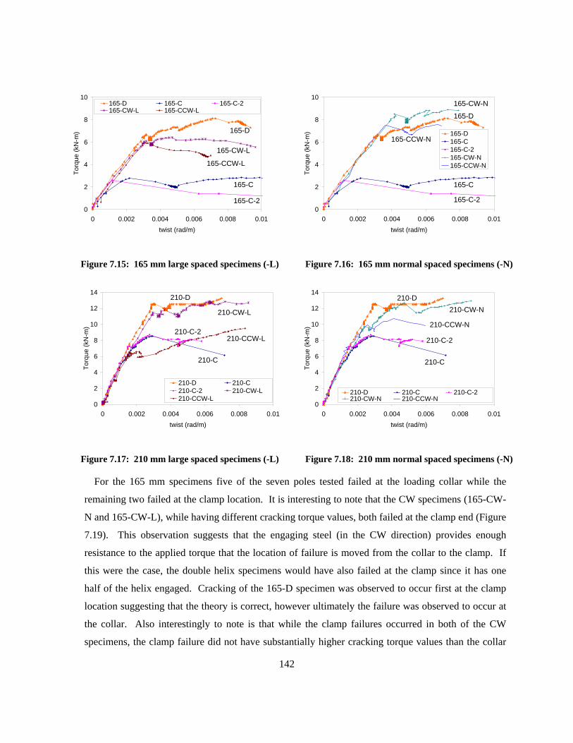
142

0

2

4

6

8

10

0 0.002 0.004 0.006 0.008 0.01twist (rad/m)

Torq

ue (k

N-m

)

165-D 165-C 165-C-2165-CW-L 165-CCW-L

165-C

165-C-2

165-CCW-L

165-D

165-CW-L

Figure 7.15: 165 mm large spaced specimens (-L)

0

2

4

6

8

10

0 0.002 0.004 0.006 0.008 0.01twist (rad/m)

Torq

ue (k

N-m

) 165-D165-C165-C-2165-CW-N165-CCW-N

165-C-2

165-CCW-N

165-D

165-CW-N

165-C

Figure 7.16: 165 mm normal spaced specimens (-N)

0

2

4

6

8

10

12

14

0 0.002 0.004 0.006 0.008 0.01twist (rad/m)

Torq

ue (k

N-m

)

210-D 210-C210-C-2 210-CW-L210-CCW-L

210-C

210-C-2

210-D

210-CW-L

210-CCW-L

Figure 7.17: 210 mm large spaced specimens (-L)

0

2

4

6

8

10

12

14

0 0.002 0.004 0.006 0.008 0.01twist (rad/m)

Torq

ue (k

N-m

)

210-D 210-C 210-C-2210-CW-N 210-CCW-N

210-C

210-C-2

210-D210-CW-N

210-CCW-N

Figure 7.18: 210 mm normal spaced specimens (-N)

For the 165 mm specimens five of the seven poles tested failed at the loading collar while the

remaining two failed at the clamp location. It is interesting to note that the CW specimens (165-CW-

N and 165-CW-L), while having different cracking torque values, both failed at the clamp end (Figure

7.19). This observation suggests that the engaging steel (in the CW direction) provides enough

resistance to the applied torque that the location of failure is moved from the collar to the clamp. If

this were the case, the double helix specimens would have also failed at the clamp since it has one

half of the helix engaged. Cracking of the 165-D specimen was observed to occur first at the clamp

location suggesting that the theory is correct, however ultimately the failure was observed to occur at

the collar. Also interestingly to note is that while the clamp failures occurred in both of the CW

specimens, the clamp failure did not have substantially higher cracking torque values than the collar

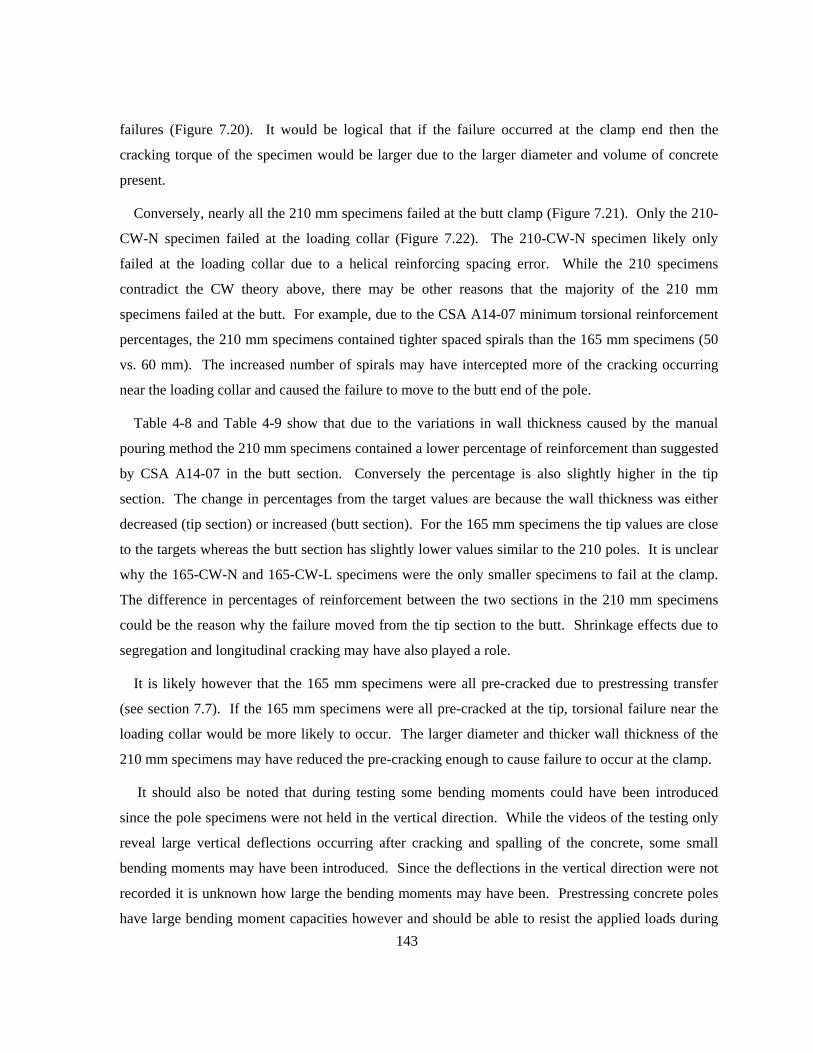
143

failures (Figure 7.20). It would be logical that if the failure occurred at the clamp end then the

cracking torque of the specimen would be larger due to the larger diameter and volume of concrete

present.

Conversely, nearly all the 210 mm specimens failed at the butt clamp (Figure 7.21). Only the 210-

CW-N specimen failed at the loading collar (Figure 7.22). The 210-CW-N specimen likely only

failed at the loading collar due to a helical reinforcing spacing error. While the 210 specimens

contradict the CW theory above, there may be other reasons that the majority of the 210 mm

specimens failed at the butt. For example, due to the CSA A14-07 minimum torsional reinforcement

percentages, the 210 mm specimens contained tighter spaced spirals than the 165 mm specimens (50

vs. 60 mm). The increased number of spirals may have intercepted more of the cracking occurring

near the loading collar and caused the failure to move to the butt end of the pole.

Table 4-8 and Table 4-9 show that due to the variations in wall thickness caused by the manual

pouring method the 210 mm specimens contained a lower percentage of reinforcement than suggested

by CSA A14-07 in the butt section. Conversely the percentage is also slightly higher in the tip

section. The change in percentages from the target values are because the wall thickness was either

decreased (tip section) or increased (butt section). For the 165 mm specimens the tip values are close

to the targets whereas the butt section has slightly lower values similar to the 210 poles. It is unclear

why the 165-CW-N and 165-CW-L specimens were the only smaller specimens to fail at the clamp.

The difference in percentages of reinforcement between the two sections in the 210 mm specimens

could be the reason why the failure moved from the tip section to the butt. Shrinkage effects due to

segregation and longitudinal cracking may have also played a role.

It is likely however that the 165 mm specimens were all pre-cracked due to prestressing transfer

(see section 7.7). If the 165 mm specimens were all pre-cracked at the tip, torsional failure near the

loading collar would be more likely to occur. The larger diameter and thicker wall thickness of the

210 mm specimens may have reduced the pre-cracking enough to cause failure to occur at the clamp.

It should also be noted that during testing some bending moments could have been introduced

since the pole specimens were not held in the vertical direction. While the videos of the testing only

reveal large vertical deflections occurring after cracking and spalling of the concrete, some small

bending moments may have been introduced. Since the deflections in the vertical direction were not

recorded it is unknown how large the bending moments may have been. Prestressing concrete poles

have large bending moment capacities however and should be able to resist the applied loads during

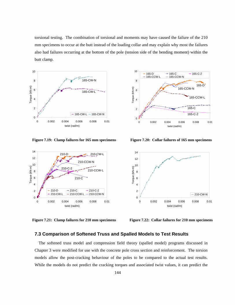
144

torsional testing. The combination of torsional and moments may have caused the failure of the 210

mm specimens to occur at the butt instead of the loading collar and may explain why most the failures

also had failures occurring at the bottom of the pole (tension side of the bending moment) within the

butt clamp.

0

2

4

6

8

10

0 0.002 0.004 0.006 0.008 0.01twist (rad/m)

Torq

ue (k

N-m

)

165-CW-L 165-CW-N

165-CW-N

165-CW-L

Figure 7.19: Clamp failures for 165 mm specimens

0

2

4

6

8

10

0 0.002 0.004 0.006 0.008 0.01twist (rad/m)

Torq

ue (k

N-m

)

165-D 165-C 165-C-2165-CCW-L 165-CCW-N

165-CCW-N

165-CCW-L

165-D

165-C-2

165-C

Figure 7.20: Collar failures of 165 mm specimens

0

2

4

6

8

10

12

14

0 0.002 0.004 0.006 0.008 0.01twist (rad/m)

Torq

ue (k

N-m

)

210-D 210-C 210-C-2210-CW-L 210-CCW-L 210-CCW-N

210-CCW-N

210-D 210-CW-L

210-CCW-L

210-C

210-C-2

Figure 7.21: Clamp failures for 210 mm specimens

0

2

4

6

8

10

12

14

0 0.002 0.004 0.006 0.008 0.01twist (rad/m)

Torq

ue (k

N-m

)

210-CW-N

Figure 7.22: Collar failures for 210 mm specimens

7.3 Comparison of Softened Truss and Spalled Models to Test Results

The softened truss model and compression field theory (spalled model) programs discussed in

Chapter 3 were modified for use with the concrete pole cross section and reinforcement. The torsion

models allow the post-cracking behaviour of the poles to be compared to the actual test results.

While the models do not predict the cracking torques and associated twist values, it can predict the

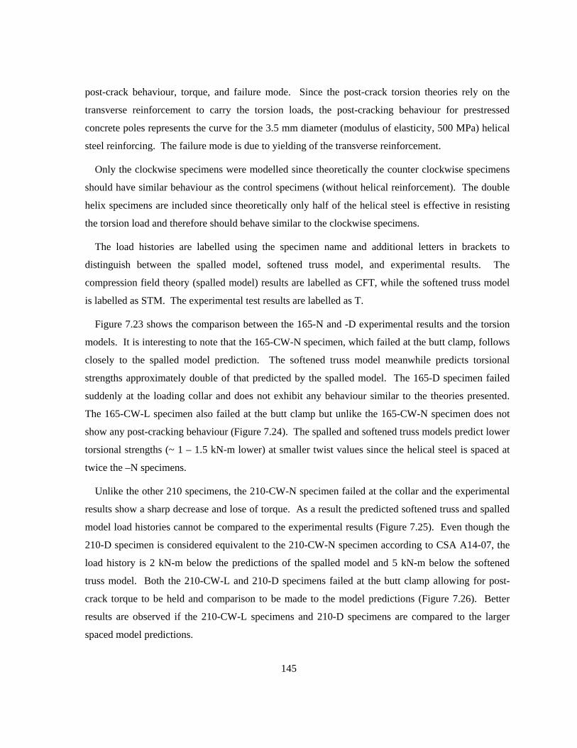
145

post-crack behaviour, torque, and failure mode. Since the post-crack torsion theories rely on the

transverse reinforcement to carry the torsion loads, the post-cracking behaviour for prestressed

concrete poles represents the curve for the 3.5 mm diameter (modulus of elasticity, 500 MPa) helical

steel reinforcing. The failure mode is due to yielding of the transverse reinforcement.

Only the clockwise specimens were modelled since theoretically the counter clockwise specimens

should have similar behaviour as the control specimens (without helical reinforcement). The double

helix specimens are included since theoretically only half of the helical steel is effective in resisting

the torsion load and therefore should behave similar to the clockwise specimens.

The load histories are labelled using the specimen name and additional letters in brackets to

distinguish between the spalled model, softened truss model, and experimental results. The

compression field theory (spalled model) results are labelled as CFT, while the softened truss model

is labelled as STM. The experimental test results are labelled as T.

Figure 7.23 shows the comparison between the 165-N and -D experimental results and the torsion

models. It is interesting to note that the 165-CW-N specimen, which failed at the butt clamp, follows

closely to the spalled model prediction. The softened truss model meanwhile predicts torsional

strengths approximately double of that predicted by the spalled model. The 165-D specimen failed

suddenly at the loading collar and does not exhibit any behaviour similar to the theories presented.

The 165-CW-L specimen also failed at the butt clamp but unlike the 165-CW-N specimen does not

show any post-cracking behaviour (Figure 7.24). The spalled and softened truss models predict lower

torsional strengths (~ 1 – 1.5 kN-m lower) at smaller twist values since the helical steel is spaced at

twice the –N specimens.

Unlike the other 210 specimens, the 210-CW-N specimen failed at the collar and the experimental

results show a sharp decrease and lose of torque. As a result the predicted softened truss and spalled

model load histories cannot be compared to the experimental results (Figure 7.25). Even though the

210-D specimen is considered equivalent to the 210-CW-N specimen according to CSA A14-07, the

load history is 2 kN-m below the predictions of the spalled model and 5 kN-m below the softened

truss model. Both the 210-CW-L and 210-D specimens failed at the butt clamp allowing for post-

crack torque to be held and comparison to be made to the model predictions (Figure 7.26). Better

results are observed if the 210-CW-L specimens and 210-D specimens are compared to the larger

spaced model predictions.

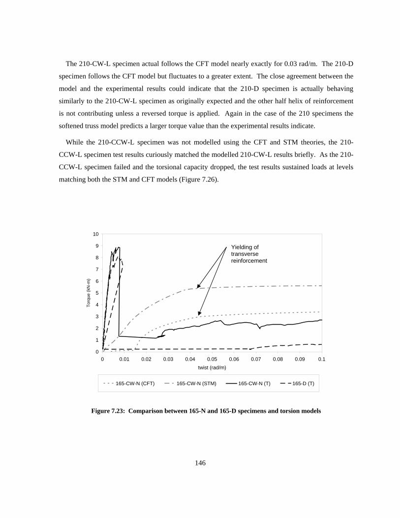
146

The 210-CW-L specimen actual follows the CFT model nearly exactly for 0.03 rad/m. The 210-D

specimen follows the CFT model but fluctuates to a greater extent. The close agreement between the

model and the experimental results could indicate that the 210-D specimen is actually behaving

similarly to the 210-CW-L specimen as originally expected and the other half helix of reinforcement

is not contributing unless a reversed torque is applied. Again in the case of the 210 specimens the

softened truss model predicts a larger torque value than the experimental results indicate.

While the 210-CCW-L specimen was not modelled using the CFT and STM theories, the 210-

CCW-L specimen test results curiously matched the modelled 210-CW-L results briefly. As the 210-

CCW-L specimen failed and the torsional capacity dropped, the test results sustained loads at levels

matching both the STM and CFT models (Figure 7.26).

0

1

2

3

4

5

6

7

8

9

10

0 0.01 0.02 0.03 0.04 0.05 0.06 0.07 0.08 0.09 0.1twist (rad/m)

Torq

ue (k

N-m

)

165-CW-N (CFT) 165-CW-N (STM) 165-CW-N (T) 165-D (T)

Figure 7.23: Comparison between 165-N and 165-D specimens and torsion models

Yielding of transverse reinforcement

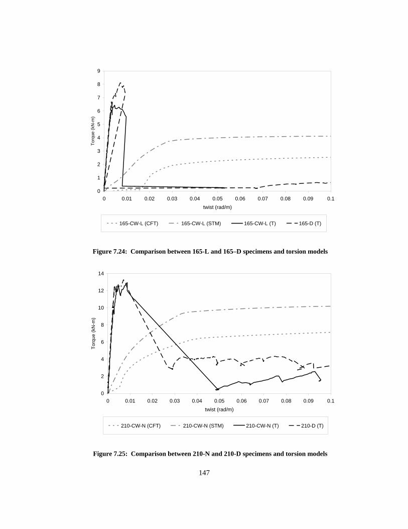
147

0

1

2

3

4

5

6

7

8

9

0 0.01 0.02 0.03 0.04 0.05 0.06 0.07 0.08 0.09 0.1twist (rad/m)

Torq

ue (k

N-m

)

165-CW-L (CFT) 165-CW-L (STM) 165-CW-L (T) 165-D (T)

Figure 7.24: Comparison between 165-L and 165–D specimens and torsion models

0

2

4

6

8

10

12

14

0 0.01 0.02 0.03 0.04 0.05 0.06 0.07 0.08 0.09 0.1twist (rad/m)

Torq

ue (k

N-m

)

210-CW-N (CFT) 210-CW-N (STM) 210-CW-N (T) 210-D (T)

Figure 7.25: Comparison between 210-N and 210-D specimens and torsion models

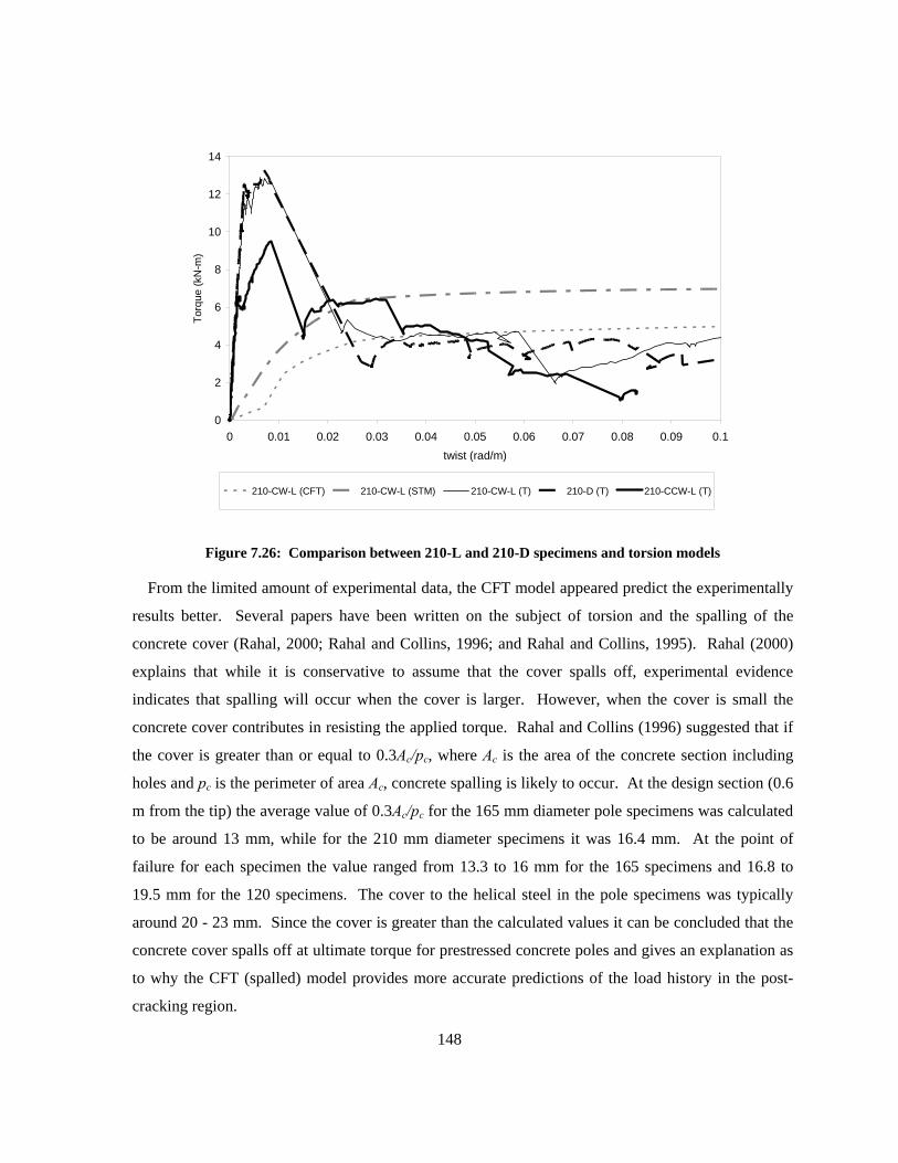
148

0

2

4

6

8

10

12

14

0 0.01 0.02 0.03 0.04 0.05 0.06 0.07 0.08 0.09 0.1twist (rad/m)

Torq

ue (k

N-m

)

210-CW-L (CFT) 210-CW-L (STM) 210-CW-L (T) 210-D (T) 210-CCW-L (T)

Figure 7.26: Comparison between 210-L and 210-D specimens and torsion models

From the limited amount of experimental data, the CFT model appeared predict the experimentally

results better. Several papers have been written on the subject of torsion and the spalling of the

concrete cover (Rahal, 2000; Rahal and Collins, 1996; and Rahal and Collins, 1995). Rahal (2000)

explains that while it is conservative to assume that the cover spalls off, experimental evidence

indicates that spalling will occur when the cover is larger. However, when the cover is small the

concrete cover contributes in resisting the applied torque. Rahal and Collins (1996) suggested that if

the cover is greater than or equal to 0.3Ac/pc, where Ac is the area of the concrete section including

holes and pc is the perimeter of area Ac, concrete spalling is likely to occur. At the design section (0.6

m from the tip) the average value of 0.3Ac/pc for the 165 mm diameter pole specimens was calculated

to be around 13 mm, while for the 210 mm diameter specimens it was 16.4 mm. At the point of

failure for each specimen the value ranged from 13.3 to 16 mm for the 165 specimens and 16.8 to

19.5 mm for the 120 specimens. The cover to the helical steel in the pole specimens was typically

around 20 - 23 mm. Since the cover is greater than the calculated values it can be concluded that the

concrete cover spalls off at ultimate torque for prestressed concrete poles and gives an explanation as

to why the CFT (spalled) model provides more accurate predictions of the load history in the post-

cracking region.

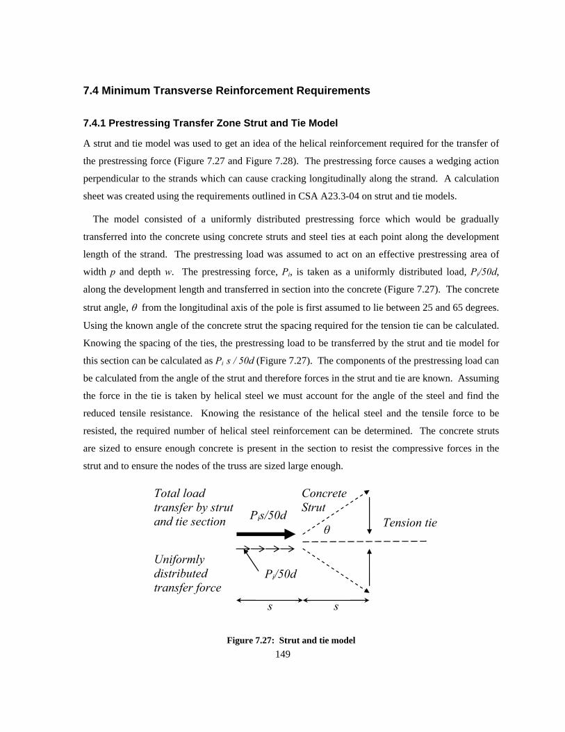
149

7.4 Minimum Transverse Reinforcement Requirements

7.4.1 Prestressing Transfer Zone Strut and Tie Model

A strut and tie model was used to get an idea of the helical reinforcement required for the transfer of

the prestressing force (Figure 7.27 and Figure 7.28). The prestressing force causes a wedging action

perpendicular to the strands which can cause cracking longitudinally along the strand. A calculation

sheet was created using the requirements outlined in CSA A23.3-04 on strut and tie models.

The model consisted of a uniformly distributed prestressing force which would be gradually

transferred into the concrete using concrete struts and steel ties at each point along the development

length of the strand. The prestressing load was assumed to act on an effective prestressing area of

width p and depth w. The prestressing force, Pi, is taken as a uniformly distributed load, Pi/50d,

along the development length and transferred in section into the concrete (Figure 7.27). The concrete

strut angle, θ from the longitudinal axis of the pole is first assumed to lie between 25 and 65 degrees.

Using the known angle of the concrete strut the spacing required for the tension tie can be calculated.

Knowing the spacing of the ties, the prestressing load to be transferred by the strut and tie model for

this section can be calculated as Pi s / 50d (Figure 7.27). The components of the prestressing load can

be calculated from the angle of the strut and therefore forces in the strut and tie are known. Assuming

the force in the tie is taken by helical steel we must account for the angle of the steel and find the

reduced tensile resistance. Knowing the resistance of the helical steel and the tensile force to be

resisted, the required number of helical steel reinforcement can be determined. The concrete struts

are sized to ensure enough concrete is present in the section to resist the compressive forces in the

strut and to ensure the nodes of the truss are sized large enough.

θ Pis/50d Tension tie

Concrete Strut

s s

Uniformly distributed transfer force

Pi/50d

Total load transfer by strut and tie section

Figure 7.27: Strut and tie model

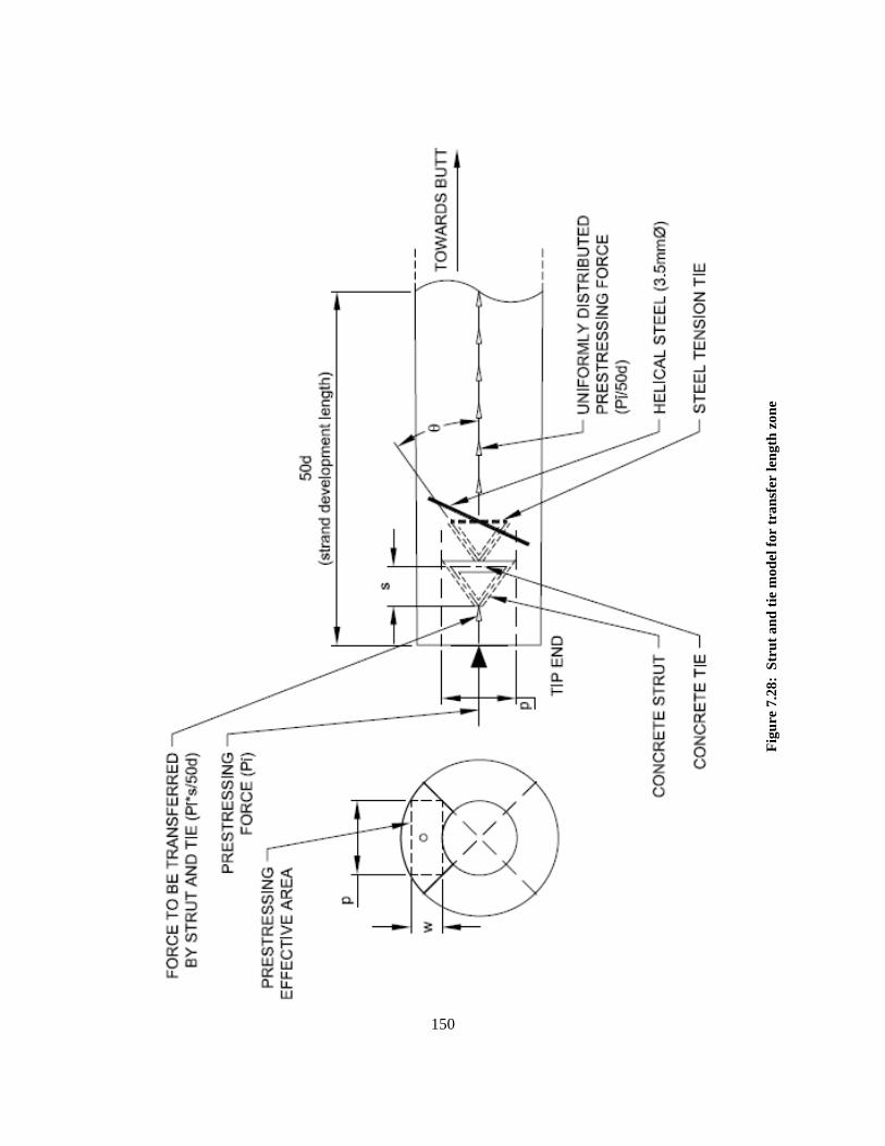
150

Figu

re 7

.28:

Str

ut a

nd ti

e m

odel

for

tran

sfer

leng

th z

one

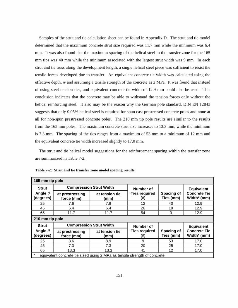
151

Samples of the strut and tie calculation sheet can be found in Appendix D. The strut and tie model

determined that the maximum concrete strut size required was 11.7 mm while the minimum was 6.4

mm. It was also found that the maximum spacing of the helical steel in the transfer zone for the 165

mm tips was 40 mm while the minimum associated with the largest strut width was 9 mm. In each

strut and tie truss along the development length, a single helical steel piece was sufficient to resist the

tensile forces developed due to transfer. An equivalent concrete tie width was calculated using the

effective depth, w and assuming a tensile strength of the concrete as 2 MPa. It was found that instead

of using steel tension ties, and equivalent concrete tie width of 12.9 mm could also be used. This

conclusion indicates that the concrete may be able to withstand the tension forces only without the

helical reinforcing steel. It also may be the reason why the German pole standard, DIN EN 12843

suggests that only 0.05% helical steel is required for spun cast prestressed concrete poles and none at

all for non-spun prestressed concrete poles. The 210 mm tip pole results are similar to the results

from the 165 mm poles. The maximum concrete strut size increases to 13.3 mm, while the minimum

is 7.3 mm. The spacing of the ties ranges from a maximum of 53 mm to a minimum of 12 mm and

the equivalent concrete tie width increased slightly to 17.0 mm.

The strut and tie helical model suggestions for the reinforcement spacing within the transfer zone

are summarized in Table 7-2.

Table 7-2: Strut and tie transfer zone model spacing results

165 mm tip pole Compression Strut Width Strut

Angle θ (degrees)

at prestressing force (mm)

at tension tie (mm)

Number of Ties required

(#) Spacing of Ties (mm)

Equivalent Concrete Tie Width* (mm)

25 7.6 7.9 12 40 12.9 45 6.4 6.4 26 19 12.9 65 11.7 11.7 54 9 12.9

210 mm tip pole Compression Strut Width Strut

Angle θ (degrees)

at prestressing force (mm)

at tension tie (mm)

Number of Ties required

(#) Spacing of Ties (mm)

Equivalent Concrete Tie Width* (mm)

25 8.6 8.9 9 53 17.0 45 7.3 7.3 20 25 17.0 65 13.3 13.3 41 12 17.0

* = equivalent concrete tie sized using 2 MPa as tensile strength of concrete

152

7.4.2 Code Required Maximum Transverse Reinforcement Spacing

To determine the spacing required for the helical steel according to the ACI-318-05, CSA A23.3-04,

and Eurocode 2 (EC2) the minimum shear reinforcement requirements presented in section 2.5 were

used. The detailed calculations of the clauses are included with the strut and tie results in Appendix

C. The calculations were done assuming the use of 3.5 mm diameter helical steel as the

transverse/torsional reinforcement. The diameter of the pole was taken as the effective width, bw.

For the 165 mm tip poles the CSA clauses suggested a maximum spacing of 62 mm whereas the

ACI and EC2 clauses suggested lower values of 51 mm and 47 mm respectively. In the case that the

factored torsional moment is larger than a quarter of the cracking torque the CSA requirement

decreases to 45.5 mm. The requirements for the 210 mm poles were lower since the effective width

increased from 165 mm to 210 mm. The CSA recommended maximum spacing for the 210 mm

poles is 49 mm while ACI and EC2 suggested 47 mm and 40 mm respectively.

The alternative equations for minimum transverse reinforcement for torsion presented by Ali and

White (1999) and Koutchoukali and Belarbi (2001) were also used to calculate the maximum spacing

permitted. The formula suggested by Ali and White gave a spacing of 19 mm for the 165 mm tip

poles and 26 mm for the 210 mm poles. Similarly, the equation suggested by Koutchoukali and

Belarbi suggested 28 and 23 mm for the 165 and 210 mm poles respectively. The equations are

developed assuming Tr = λTcr and the tighter spacing requirements suggested by these equations are

due to the assumed value λ. Ali and White and Koutchoukali and Belarbi assumed a value greater

than 1 for λ. If λ is assumed to be 1 and the calculations are repeated for maximum spacing of the

transverse reinforcement a value of 36 mm results for the 165 mm poles and 29 for the 210 mm poles.

In either case the transverse reinforcement equations presented in the literature give tighter spacing

requirements than the codes. It is possible that theses equations should only be used for large

concrete members and cannot be used in the case of prestressed concrete poles. It should also be

noted that a spacing of less than 20 mm is not feasible for manufacturing purposes since concrete

must be able to pass through the helical reinforcing during pouring and spinning of the concrete pole.

Similar to the strut and tie model results, the helical reinforcement spacing for all experimental

specimens were all larger than the recommended concrete code maximum transverse reinforcement

spacing.

153

7.5 Comparison of Experimental and Theoretical Cracking Torque Results

During the design of the specimens (section 4.4) it was noted that the equations given in the CSA

A23.3-04 (2004) and ACI 318-05 (2005) code for ultimate torsional capacity resulted in lower values

than the values based on the cracking torque formulae. The ultimate torsional capacity equations are

not really applicable since they are based on the space truss model and are dependent on the

transverse/helical reinforcing steel and ignore the concrete contribution. In the case of prestressed

concrete poles, the helical reinforcing steel area is so small that the calculated ultimate torsional

capacity is lower than the cracking torque, indicating that the poles fail at cracking loads. Given this,

the equations presented in section 2.4.2 were not used.

Using the cracking torque formulae presented in section 2.4.1, a comparison between theoretical

and experimental results were made. The experimental cracking torque (taken at the point when the

torque-twist curve became non-linear) was used for comparison as well as the maximum torque

sustained by each specimen. In addition, comparisons were made at the theoretical minimum

torsional resistance location on the pole at 0.6 m from the tip (Table 7-3, Table 7-5) and at the

recorded failure location (loading collar or butt clamp) using the measured wall thickness at the

failure location (Table 7-4, Table 7-6). The same tables were then reproduced using two different

sets of prestressing values. The first set was calculated from measurements taken of the strand

elongation between the initial prestressing to tighten the strand and the final prestressing during

manufacturing (Table 7-3 and Table 7-4). The measured change in length of the strands, recorded by

the manufacturers was typically around 140 mm. Using the strand elongation measurements and

taking into account the length changes in the pole mould and tip/butt plates prestressing stresses were

calculated for each specimen. Since the stressing jack doesn’t allow overstressing, theoretically each

pole should have been stressed to the same prestressing value. The second prestressing value used for

all pole specimens assumed a prestressing stress of 0.8fpu and final prestressing losses of 21% as

given in codes (Table 7-5 and Table 7-6).

Ratios of experimental to theoretical values were produced to predict the accuracy and

conservativeness of each formula. Statistical information presented below the tables allows for

comparison between the theoretical methods. Figure 7.29, Figure 7.30, and Figure 7.31 summarize

the predictions by ACI 318-05, CSA A23.3-04 and EC2 respectively. The code summarizes provide

a visual interpretation of the Table 7-3 to Table 7-6. Ratios above 1.0 in the tables and figures

represent a conservative code prediction of the experimental cracking torque.

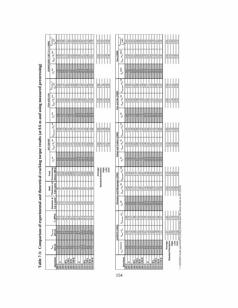
154

Tab

le 7

-3:

Com

pari

son

of e

xper

imen

tal a

nd th

eore

tical

cra

ckin

g to

rque

res

ults

(at 0

.6 m

and

usi

ng m

easu

red

pres

tres

sing

)

T crAC

IT t

est /

Tcr

ACI

T tes

t-max

/ T c

rAC

IT c

rCSA

T tes

t / T

crC

SAT t

est-m

ax /

T crC

SAT c

rEC2

T tes

t / T

crEC

2T t

est-m

ax /

T crEC

2

165-

C2.

82.

850

.617

446

1116

6.3

0.44

0.45

6.8

0.41

0.42

7.9

0.35

0.36

165-

C-2

2.6

2.6

72.3

174

4710

706.

80.

370.

387.

40.

340.

358.

80.

290.

2916

5-D

6.7

8.1

66.4

174

4910

596.

61.

021.

237.

10.

941.

148.

40.

790.

9616

5-C

W-L

6.1

6.4

64.7

174

4810

526.

50.

930.

987.

10.

860.

918.

40.

730.

7716

5-C

CW

-L5.

95.

945

.817

449

1059

5.9

1.01

1.01

6.4

0.93

0.93

7.2

0.83

0.83

165-

CW

-N8.

58.

963

.717

450

1089

6.5

1.31

1.36

7.1

1.21

1.26

8.3

1.02

1.07

165-

CC

W-N

7.5

7.5

66.0

174

4810

596.

61.

141.

147.

11.

051.

068.

50.

890.

8921

0-C

5.1

8.5

61.5

219

4811

1611

.60.

440.

7312

.60.

400.

6814

.10.

360.

6021

0-C

-27.

38.

768

.121

953

1070

11.5

0.64

0.76

12.5

0.58

0.70

14.6

0.50

0.59

210-

D12

.513

.365

.321

955

1059

11.2

1.12

1.19

12.2

1.03

1.09

14.4

0.87

0.92

210-

CW

-L11

.512

.962

.621

953

1052

11.1

1.03

1.16

12.1

0.95

1.07

14.1

0.81

0.91

210-

CC

W-L

6.5

9.5

57.0

219

5710

5910

.60.

620.

8911

.60.

570.

8213

.60.

480.

7021

0-C

W-N

9.8

12.9

67.5

219

5310

8911

.50.

851.

1212

.50.

781.

0314

.70.

670.

8821

0-C

CW

-N7.

110

.763

.621

958

1059

10.9

0.65

0.98

11.9

0.60

0.90

14.1

0.51

0.76

Ave

rage

:0.

830.

960.

760.

880.

650.

75St

anda

rd D

evia

tion:

0.30

0.29

0.28

0.27

0.23

0.22

Hig

h:1.

311.

361.

211.

261.

021.

07Lo

w:

0.37

0.38

0.34

0.35

0.29

0.29

CO

V:0.

360.

300.

360.

300.

360.

30

T crA

ASH

TO,9

4T t

est /

Tcr

T tes

t-max

/ T c

rT c

rGM

T tes

t / T

crG

MT t

est-m

ax /

T crG

MT c

rRC

T tes

t / T

crR

CT t

est-m

ax /

T crR

CT c

rHM

T tes

t / T

crH

MT t

est-m

ax /

T crH

MT c

rHM

eff

T tes

t / T

crH

Mef

fT t

est-m

ax /

T crH

Mef

f

165-

C2.

90.

960.

998.

20.

340.

347.

20.

390.

406.

20.

450.

466.

40.

430.

4416

5-C

-23.

40.

740.

759.

00.

280.

297.

80.

330.

337.

40.

350.

357.

60.

330.

3416

5-D

3.3

2.04

2.47

8.6

0.78

0.94

7.5

0.89

1.08

7.2

0.93

1.12

13.0

0.52

0.63

165-

CW

-L3.

21.

881.

988.

50.

710.

757.

40.

820.

867.

10.

860.

9110

.00.

610.

6416

5-C

CW

-L2.

72.

172.

177.

70.

770.

776.

70.

880.

886.

00.

980.

988.

50.

690.

6916

5-C

W-N

3.2

2.65

2.76

8.5

1.00

1.04

7.4

1.14

1.19

7.3

1.16

1.21

13.2

0.65

0.68

165-

CC

W-N

3.3

2.29

2.30

8.6

0.87

0.87

7.5

1.00

1.00

7.1

1.05

1.06

12.8

0.59

0.59

210-

C6.

30.

811.

3515

.20.

330.

5613

.30.

380.

6410

.00.

510.

8510

.30.

490.

8321

0-C

-26.

61.

101.

3115

.10.

480.

5813

.20.

550.

6611

.20.

650.

7711

.50.

640.

7621

0-D

6.5

1.93

2.05

14.7

0.85

0.90

12.9

0.97

1.03

11.2

1.11

1.18

23.1

0.54

0.58

210-

CW

-L6.

41.

802.

0214

.60.

790.

8812

.80.

901.

0110

.71.

071.

2016

.50.

700.

7821

0-C

CW

-L6.

11.

081.

5714

.00.

470.

6812

.20.

530.

7810

.80.

610.

8816

.60.

400.

5721

0-C

W-N

6.6

1.48

1.96

15.2

0.64

0.85

13.3

0.74

0.98

11.2

0.87

1.16

23.0

0.42

0.56

210-

CC

W-N

6.4

1.11

1.67

14.4

0.49

0.74

12.6

0.56

0.85

11.6

0.61

0.92

23.8

0.30

0.45

Ave

rage

:1.

571.

810.

630.

730.

720.

830.

800.

930.

520.

61St

anda

rd D

evia

tion:

0.61

0.57

0.23

0.22

0.26

0.25

0.27

0.27

0.13

0.14

Hig

h:2.

652.

761.

001.

041.

141.

191.

161.

210.

700.

83Lo

w:

0.74

0.75

0.28

0.29

0.33

0.33

0.35

0.35

0.30

0.34

CO

V:0.

390.

310.

360.

300.

360.

300.

340.

280.

250.

22* =

AS

CE/

PCI G

uide

and

AAS

HTO

(200

1) fo

rmul

as g

ive

the

sam

e re

sults

as

ACI 3

18-0

5

Hsu

(196

8)

AC

I 318

-05*

Dia

met

er a

t 0.

6 m

(mm

)

Wal

l Th

ickn

ess

at

0.6m

(mm

)

Gho

neim

and

Mac

greg

or (1

993)

Fin

al

Pres

tres

sing

St

ress

(MPa

)Sp

ecim

enT t

est

(kN

-m)

T tes

t-max

(kN

-m)

f' c (M

Pa)

Rah

al a

nd C

ollin

s (1

996)

Hsu

and

Mo

(198

5)A

ASH

TO (1

994)

S pec

imen

CSA

-A23

.3-0

4EU

RO

CO

DE

2 (E

C 2

-1-1

:200

4)

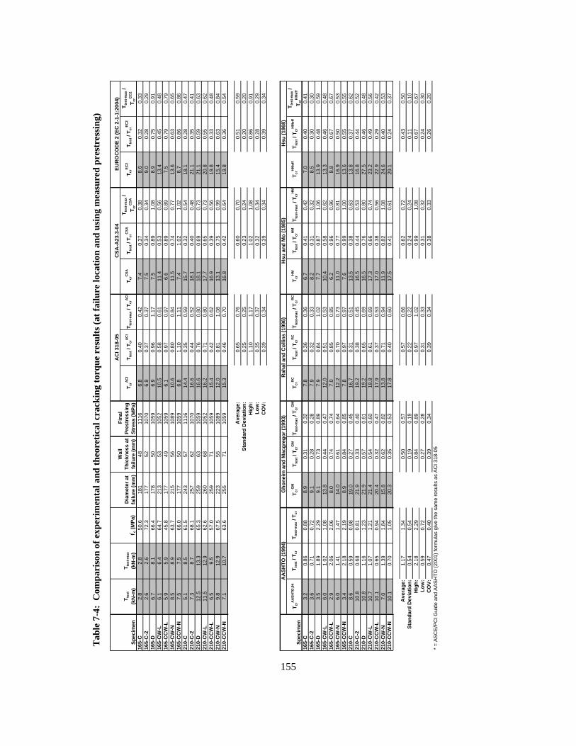
155

Tab

le 7

-4:

Com

pari

son

of e

xper

imen

tal a

nd th

eore

tical

cra

ckin

g to

rque

res

ults

(at f

ailu

re lo

catio

n an

d us

ing

mea

sure

d pr

estr

essi

ng)

T crAC

IT t

est /

Tcr

ACI

T tes

t-max

/ T c

rACI

T crC

SAT t

est /

Tcr

CSA

T tes

t-max

/ T c

rCSA

T crEC

2T t

est /

Tcr

EC2

T tes

t-max

/ T c

rEC2

165-

C2.

82.

850

.618

148

1116

6.8

0.40

0.42

7.4

0.37

0.38

8.6

0.32

0.33

165-

C-2

2.6

2.6

72.3

177

5210

706.

90.

370.

377.

50.

340.

349.

00.

280.

2916

5-D

6.7

8.1

66.4

178

5010

596.

90.

961.

177.

50.

891.

088.

90.

750.

9116

5-C

W-L

6.1

6.4

64.7

213

5310

5210

.50.

580.

6111

.40.

530.

5613

.40.

450.

4816

5-C

CW

-L5.

95.

945

.817

749

1059

6.1

0.97

0.97

6.6

0.89

0.89

7.5

0.79

0.79

165-

CW

-N8.

58.

963

.721

556

1089

10.6

0.80

0.84

11.5

0.74

0.77

13.6

0.63

0.65

165-

CC

W-N

7.5

7.5

66.0

177

5010

596.

81.

101.

117.

41.

021.

028.

70.

860.

8621

0-C

5.1

8.5

61.5

243

5711

1614

.40.

350.

5915

.70.

320.

5418

.10.

280.

4721

0-C

-27.

38.

768

.125

762

1070

16.6

0.44

0.52

18.1

0.40

0.48

21.1

0.35

0.41

210-

D12

.513

.365

.325

963

1059

16.6

0.76

0.80

18.1

0.69

0.73

21.1

0.59

0.63

210-

CW

-L11

.512

.962

.626

068

1052

16.2

0.71

0.80

17.7

0.65

0.73

20.8

0.55

0.62

210-

CC

W-L

6.5

9.5

57.0

259

7110

5915

.40.

420.

6216

.90.

390.

5619

.80.

330.

4821

0-C

W-N

9.8

12.9

67.5

223

5510

8912

.00.

811.

0813

.10.

750.

9915

.40.

630.

8421

0-C

CW

-N7.

110

.763

.625

571

1059

15.3

0.46

0.70

16.8

0.42

0.64

19.8

0.36

0.54

Ave

rage

:0.

650.

760.

600.

700.

510.

59St

anda

rd D

evia

tion:

0.25

0.25

0.23

0.24

0.20

0.20

Hig

h:1.

101.

171.

021.

080.

860.

91Lo

w:

0.35

0.37

0.32

0.34

0.28

0.29

CO

V:0.

390.

340.

390.

340.

390.

34

T crA

ASH

TO,9

4T t

est /

Tcr

T tes

t-max

/ T c

rT c

rGM

T tes

t / T

crG

MT t

est-m

ax /

T crG

MT c

rRC

T tes

t / T

crR

CT t

est-m

ax /

T crR

CT c

rHM

T tes

t / T

crH

MT t

est-m

ax /

T crH

MT c

rHM

eff

T tes

t / T

crH

Mef

fT t

est-m

ax /

T crH

Mef

f

165-

C3.

20.

860.

888.

90.

310.

327.

80.

360.

366.

70.

410.

427.

00.

400.

4116

5-C

-23.

60.

710.

729.

10.

280.

287.

90.

320.

338.

20.

310.

328.

50.

300.

3016

5-D

3.5

1.89

2.29

9.1

0.73

0.89

7.9

0.84

1.02

7.7

0.87

1.06

13.9

0.48

0.59

165-

CW

-L6.

01.

021.

0813

.80.

440.

4712

.00.

510.

5310

.40.

580.

6213

.30.

460.

4816

5-C

CW

-L2.

92.

062.

068.

00.

740.

747.

00.

850.

856.

20.

960.

968.

80.

670.

6716

5-C

W-N

6.0

1.41

1.47

14.0

0.61

0.64

12.2

0.70

0.73

11.0

0.77

0.81

16.9

0.50

0.53

165-

CC

W-N

3.4

2.18

2.19

8.9

0.84

0.85

7.8

0.97

0.97

7.6

0.99

1.00

13.6

0.55

0.55

210-

C8.

60.

590.

9819

.00.

270.

4516

.70.

310.

5113

.50.

380.

6313

.80.

370.

6221

0-C

-210

.80.

680.

8121

.90.

330.

4019

.20.

380.

4516

.50.

440.

5316

.80.

440.

5221

0-D

10.8

1.16

1.23

21.9

0.57

0.61

19.2

0.65

0.69

16.5

0.76

0.80

27.5

0.46

0.48

210-

CW

-L10

.71.

071.

2121

.40.

540.

6018

.80.

610.

6917

.30.

660.

7423

.20.

490.

5621

0-C

CW

-L10

.10.

650.

9420

.40.

320.

4717

.90.

370.

5317

.00.

380.

5622

.90.

290.

4221

0-C

W-N

7.0

1.39

1.84

15.8

0.62

0.82

13.8

0.71

0.94

11.9

0.82

1.08

24.6

0.40

0.53

210-

CC

W-N

10.1

0.70

1.05

20.3

0.35

0.53

17.8

0.40

0.60

17.5

0.41

0.61

29.1

0.24

0.37

Ave

rage

:1.

171.

340.

500.

570.

570.

660.

620.

720.

430.

50St

anda

rd D

evia

tion:

0.54

0.54

0.19

0.19

0.22

0.22

0.24

0.24

0.11

0.10

Hig

h:2.

182.

290.

840.

890.

971.

020.

991.

080.

670.

67Lo

w:

0.59

0.72

0.27

0.28

0.31

0.33

0.31

0.32

0.24

0.30

CO

V:0.

470.

400.

390.

340.

390.

340.

380.

330.

260.

20* =

AS

CE/

PCI G

uide

and

AAS

HTO

(200

1) fo

rmul

as g

ive

the

sam

e re

sults

as

AC

I 318

-05

Hsu

(196

8)

Spec

imen

T tes

t

(kN

-m)

T tes

t-max

(kN

-m)

f' c (M

Pa)

Dia

met

er a

t fa

ilure

(mm

)

Wal

l Th

ickn

ess

at

failu

re (m

m)

EUR

OC

OD

E 2

(EC

2-1

-1:2

004)

Fin

al

Pres

tres

sing

St

ress

(MPa

)

CSA

-A23

.3-0

4

S pec

imen

AA

SHTO

(199

4)G

hone

im a

nd M

acgr

egor

(199

3)R

ahal

and

Col

lins

(199

6)H

su a

nd M

o (1

985)

AC

I 318

-05

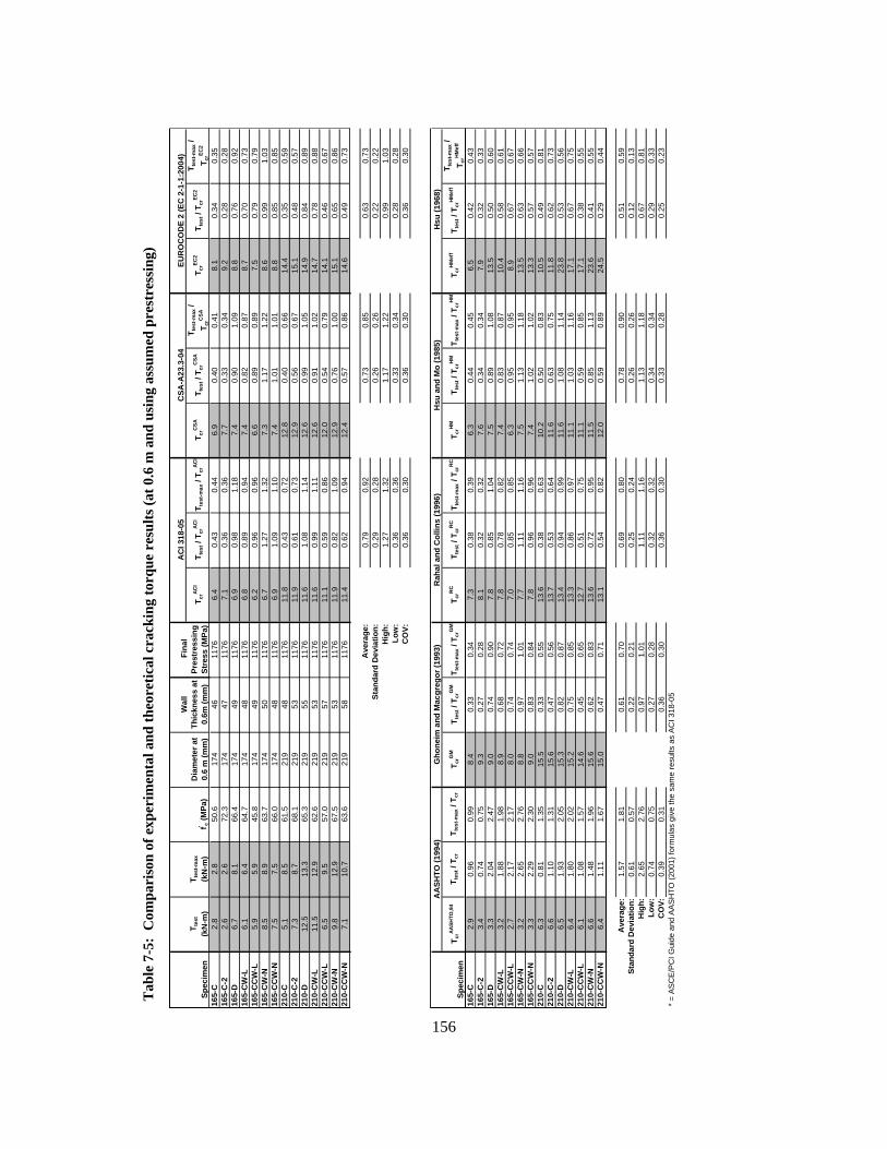
156

Tab

le 7

-5:

Com

pari

son

of e

xper

imen

tal a

nd th

eore

tical

cra

ckin

g to

rque

res

ults

(at 0

.6 m

and

usi

ng a

ssum

ed p

rest

ress

ing)

T crAC

IT t

est /

Tcr

AC

IT t

est-m

ax /

T crA

CI

T crC

SAT t

est /

Tcr

CSA

T tes

t-max

/ T c

rCSA

T crEC

2T t

est /

Tcr

EC2

T tes

t-max

/ T c

rEC2

165-

C2.

82.

850

.617

446

1176

6.4

0.43

0.44

6.9

0.40

0.41

8.1

0.34

0.35

165-

C-2

2.6

2.6

72.3

174

4711

767.

10.

360.

367.

70.

330.

349.

20.

280.

2816

5-D

6.7

8.1

66.4

174

4911

766.

90.

981.

187.

40.

901.

098.

80.

760.

9216

5-C

W-L

6.1

6.4

64.7

174

4811

766.

80.

890.

947.

40.

820.

878.

70.

700.

7316

5-C

CW

-L5.

95.

945

.817

449

1176

6.2

0.96

0.96

6.6

0.89

0.89

7.5

0.79

0.79

165-

CW

-N8.

58.

963

.717

450

1176

6.7

1.27

1.32

7.3

1.17

1.22

8.6

0.99

1.03

165-

CC

W-N

7.5

7.5

66.0

174

4811

766.

91.

091.

107.

41.

011.

018.

80.

850.

8521

0-C

5.1

8.5

61.5

219

4811

7611

.80.

430.

7212

.80.

400.

6614

.40.

350.

5921

0-C

-27.

38.

768

.121

953

1176

11.9

0.61

0.73

12.9

0.56

0.67

15.1

0.48

0.57

210-

D12

.513

.365

.321

955

1176

11.6

1.08

1.14

12.6

0.99

1.05

14.9

0.84

0.89

210-

CW

-L11

.512

.962

.621

953

1176

11.6

0.99

1.11

12.6

0.91

1.02

14.7

0.78

0.88

210-

CC

W-L

6.5

9.5

57.0

219

5711

7611

.10.

590.

8612

.00.

540.

7914

.10.

460.

6721

0-C

W-N

9.8

12.9

67.5

219

5311

7611

.90.

821.

0912

.90.

761.

0015

.10.

650.

8621

0-C

CW

-N7.

110

.763

.621

958

1176

11.4

0.62

0.94

12.4

0.57

0.86

14.6

0.49

0.73

Ave

rage

:0.

790.

920.

730.

850.

630.

73St

anda

rd D

evia

tion:

0.29

0.28

0.26

0.26

0.22

0.22

Hig

h:1.

271.

321.

171.

220.

991.

03Lo

w:

0.36

0.36

0.33

0.34

0.28

0.28

CO

V:0.

360.

300.

360.

300.

360.

30

T crAA

SHTO

,94

T tes

t / T

crT t

est-m

ax /

T cr

T crG

MT t

est /

Tcr

GM

T tes

t-max

/ T c

rGM

T crR

CT t

est /

Tcr

RC

T tes

t-max

/ T c

rRC

T crH

MT t

est /

Tcr

HM

T tes

t-max

/ T c

rHM

T crH

Mef

fT t

est /

Tcr

HM

eff

T tes

t-max

/ T c

rHM

eff

165-

C2.

90.

960.

998.

40.

330.

347.

30.

380.

396.

30.

440.

456.

50.

420.

4316

5-C

-23.

40.

740.

759.

30.

270.

288.

10.

320.

327.

60.

340.

347.

90.

320.

3316

5-D

3.3

2.04

2.47

9.0

0.74

0.90

7.8

0.85

1.04

7.5

0.89

1.08

13.5

0.50

0.60

165-

CW

-L3.

21.

881.

988.

90.

680.

727.

80.

780.

827.

40.

830.

8710

.40.

580.

6116

5-C

CW

-L2.

72.

172.

178.

00.

740.

747.

00.

850.

856.

30.

950.

958.

90.

670.

6716

5-C

W-N

3.2

2.65

2.76

8.8

0.97

1.01

7.7

1.11

1.16

7.5

1.13

1.18

13.5

0.63

0.66

165-

CC

W-N

3.3

2.29

2.30

9.0

0.83

0.84

7.8

0.96

0.96

7.4

1.02

1.02

13.3

0.57

0.57

210-

C6.

30.

811.

3515

.50.

330.

5513

.60.

380.

6310

.20.

500.

8310

.50.

490.

8121

0-C

-26.

61.

101.

3115

.60.

470.

5613

.70.

530.

6411

.60.

630.

7511

.80.

620.

7321

0-D

6.5

1.93

2.05

15.3

0.82

0.87

13.4

0.94

0.99

11.6

1.08

1.14

23.8

0.53

0.56

210-

CW

-L6.

41.

802.

0215

.20.

750.

8513

.30.

860.

9711

.11.

031.

1617

.10.

670.

7521

0-C

CW

-L6.

11.

081.

5714

.60.

450.

6512

.70.

510.

7511

.10.

590.

8517

.10.

380.

5521

0-C

W-N

6.6

1.48

1.96

15.6

0.62

0.83

13.6

0.72

0.95

11.5

0.85

1.13

23.6

0.41

0.55

210-

CC

W-N

6.4

1.11

1.67

15.0

0.47

0.71

13.1

0.54

0.82

12.0

0.59

0.89

24.5

0.29

0.44

Ave

rage

:1.

571.

810.

610.

700.

690.

800.

780.

900.

510.

59St

anda

rd D

evia

tion:

0.61

0.57

0.22

0.21

0.25

0.24

0.26

0.26

0.12

0.13

Hig

h:2.

652.

760.

971.

011.

111.

161.

131.

180.

670.

81Lo

w:

0.74

0.75

0.27

0.28

0.32

0.32

0.34

0.34

0.29

0.33

CO

V:0.

390.

310.

360.

300.

360.

300.

330.

280.

250.

23* =

ASC

E/P

CI G

uide

and

AAS

HTO

(200

1) fo

rmul

as g

ive

the

sam

e re

sults

as

ACI 3

18-0

5

Hsu

(196

8)

AC

I 318

-05

Dia

met

er a

t 0.

6 m

(mm

)

Wal

l Th

ickn

ess

at

0.6m

(mm

)

Gho

neim

and

Mac

greg

or (1

993)

Fin

al

Pres

tres

sing

St

ress

(MPa

)Sp

ecim

enT t

est

(kN

-m)

T tes

t-max

(kN

-m)

f' c (M

Pa)

Rah

al a

nd C

ollin

s (1

996)

Hsu

and

Mo

(198

5)A

ASH

TO (1

994)

S pec

imen

CSA

-A23

.3-0

4EU

RO

CO

DE

2 (E

C 2

-1-1

:200

4)

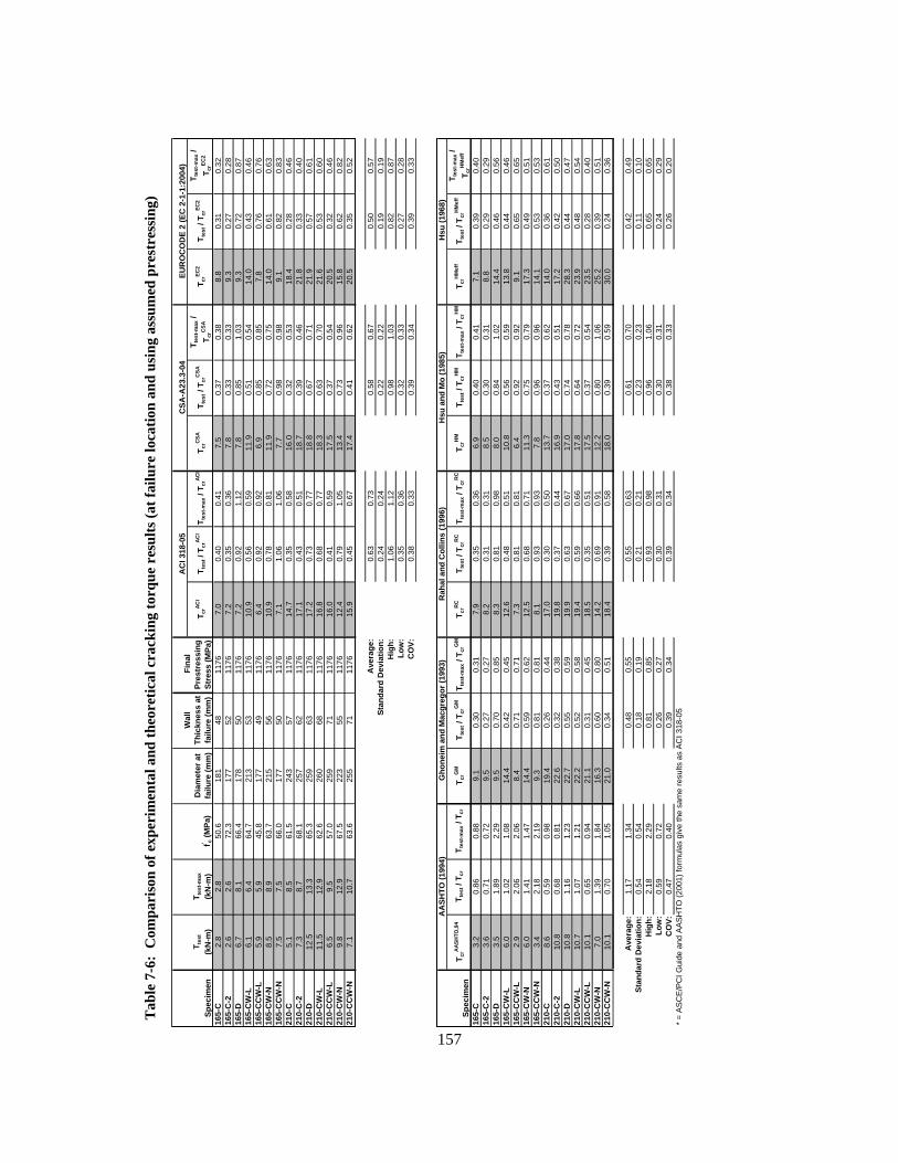
157

Tab

le 7

-6:

Com

pari

son

of e

xper

imen

tal a

nd th

eore

tical

cra

ckin

g to

rque

res

ults

(at f

ailu

re lo

catio

n an

d us

ing

assu

med

pre

stre

ssin

g)

T crAC

IT t

est /

Tcr

AC

IT t

est-m

ax /

T crAC

IT c

rCSA

T tes

t / T

crC

SAT t

est-m

ax /

T crC

SAT c

rEC2

T tes

t / T

crEC

2T t

est-m

ax /

T crEC

2

165-

C2.

82.

850

.618

148

1176

7.0

0.40

0.41

7.5

0.37

0.38

8.8

0.31

0.32

165-

C-2

2.6

2.6

72.3

177

5211

767.

20.

350.

367.

80.

330.

339.

30.

270.

2816

5-D

6.7

8.1

66.4

178

5011

767.

20.

921.

127.

80.

851.

039.

30.

720.

8716

5-C

W-L

6.1

6.4

64.7

213

5311

7610

.90.

560.

5911

.90.

510.

5414

.00.

430.

4616

5-C

CW

-L5.

95.

945

.817

749

1176

6.4

0.92

0.92

6.9

0.85

0.85

7.8

0.76

0.76

165-

CW

-N8.

58.

963

.721

556

1176

10.9

0.78

0.81

11.9

0.72

0.75

14.0

0.61

0.63

165-

CC

W-N

7.5

7.5

66.0

177

5011

767.

11.

061.

067.

70.

980.

989.

10.

820.

8321

0-C

5.1

8.5

61.5

243

5711

7614

.70.

350.

5816

.00.

320.

5318

.40.

280.

4621

0-C

-27.

38.

768

.125

762

1176

17.1

0.43

0.51

18.7

0.39

0.46

21.8

0.33

0.40

210-

D12

.513

.365

.325

963

1176

17.2

0.73

0.77

18.8

0.67

0.71

21.9

0.57

0.61

210-

CW

-L11

.512

.962

.626

068

1176

16.8

0.68

0.77

18.3

0.63

0.70

21.6

0.53

0.60

210-

CC

W-L

6.5

9.5

57.0

259

7111

7616

.00.

410.

5917

.50.

370.

5420

.50.

320.

4621

0-C

W-N

9.8

12.9

67.5

223

5511

7612

.40.

791.

0513

.40.

730.

9615

.80.

620.

8221

0-C

CW

-N7.

110

.763

.625

571

1176

15.9

0.45

0.67

17.4

0.41

0.62

20.5

0.35

0.52

Ave

rage

:0.

630.

730.

580.

670.

500.

57St

anda

rd D

evia

tion:

0.24

0.24

0.22

0.22

0.19

0.19

Hig

h:1.

061.

120.

981.

030.

820.

87Lo

w:

0.35

0.36

0.32

0.33

0.27

0.28

CO

V:0.

380.

330.

390.

340.

390.

33

T crA

ASH

TO,9

4T t

est /

Tcr

T tes

t-max

/ T c

rT c

rGM

T tes

t / T

crG

MT t

est-m

ax /

T crG

MT c

rRC

T tes

t / T

crR

CT t

est-m

ax /

T crR

CT c

rHM

T tes

t / T

crH

MT t

est-m

ax /

T crH

MT c

rHM

eff

T tes

t / T

crH

Mef

fT t

est-m

ax /

T crH

Mef

f

165-

C3.

20.

860.

889.

10.

300.

317.

90.

350.

366.

90.

400.

417.

10.

390.

4016

5-C

-23.

60.

710.

729.

50.

270.

278.

20.

310.

318.

50.

300.

318.

80.

290.

2916

5-D

3.5

1.89

2.29

9.5

0.70

0.85

8.3

0.81

0.98

8.0

0.84

1.02

14.4

0.46

0.56

165-

CW

-L6.

01.

021.

0814

.40.

420.

4512

.60.

480.

5110

.80.

560.

5913

.80.

440.

4616

5-C

CW

-L2.

92.

062.

068.

40.

710.

717.

30.

810.

816.

40.

920.

929.

10.

650.

6516

5-C

W-N

6.0

1.41

1.47

14.4

0.59

0.62

12.5

0.68

0.71

11.3

0.75

0.79

17.3

0.49

0.51

165-

CC

W-N

3.4

2.18

2.19

9.3

0.81

0.81

8.1

0.93

0.93

7.8

0.96

0.96

14.1

0.53

0.53

210-

C8.

60.

590.

9819

.40.

260.

4417

.00.

300.

5013

.70.

370.

6214

.00.

360.

6121

0-C

-210

.80.

680.

8122

.60.

320.

3819

.80.

370.

4416

.90.

430.

5117

.20.

420.

5021

0-D

10.8

1.16

1.23

22.7

0.55

0.59

19.9

0.63

0.67

17.0

0.74

0.78

28.3

0.44

0.47

210-

CW

-L10

.71.

071.

2122

.20.

520.

5819

.40.

590.

6617

.80.

640.

7223

.90.

480.

5421

0-C

CW

-L10

.10.

650.

9421

.10.

310.

4518

.50.

350.

5117

.50.

370.

5423

.50.

280.

4021

0-C

W-N

7.0

1.39

1.84

16.3

0.60

0.80

14.2

0.69

0.91

12.2

0.80

1.06

25.2

0.39

0.51

210-

CC

W-N

10.1

0.70

1.05

21.0

0.34

0.51

18.4

0.39

0.58

18.0

0.39

0.59

30.0

0.24

0.36

Ave

rage

:1.

171.

340.

480.

550.

550.

630.

610.

700.

420.

49St

anda

rd D

evia

tion:

0.54

0.54

0.18

0.19

0.21

0.21

0.23

0.23

0.11

0.10

Hig

h:2.

182.

290.

810.

850.

930.

980.

961.

060.

650.

65Lo

w:

0.59

0.72

0.26

0.27

0.30

0.31

0.30

0.31

0.24

0.29

CO

V:0.

470.

400.

390.

340.

390.

340.

380.

330.

260.

20* =

AS

CE/

PCI G

uide

and

AAS

HTO

(200

1) fo

rmul

as g

ive

the

sam

e re

sults

as

ACI 3

18-0

5

Hsu

(196

8)

S pec

imen

T tes

t

(kN

-m)

T tes

t-max

(kN

-m)

f' c (M

Pa)

Dia

met

er a

t fa

ilure

(mm

)

Wal

l Th

ickn

ess

at

failu

re (m

m)

EUR

OC

OD

E 2

(EC

2-1

-1:2

004)

Fin

al

Pres

tres

sing

St

ress

(MPa

)

CSA

-A23

.3-0

4

S pec

imen

AA

SHTO

(199

4)G

hone

im a

nd M

acgr

egor

(199

3)R

ahal

and

Col

lins

(199

6)H

su a

nd M

o (1

985)

AC

I 318

-05

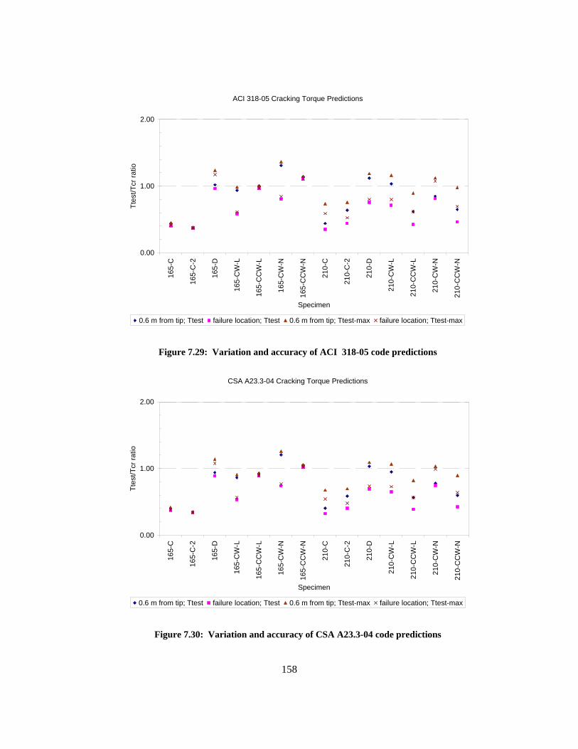
158

ACI 318-05 Cracking Torque Predictions

0.00

1.00

2.00

165-

C

165-

C-2

165-

D

165-

CW

-L

165-

CC

W-L

165-

CW

-N

165-

CC

W-N

210-

C

210-

C-2

210-

D

210-

CW

-L

210-

CC

W-L

210-

CW

-N

210-

CC

W-N

Specimen

Ttes

t/Tcr

ratio

0.6 m from tip; Ttest failure location; Ttest 0.6 m from tip; Ttest-max failure location; Ttest-max

Figure 7.29: Variation and accuracy of ACI 318-05 code predictions

CSA A23.3-04 Cracking Torque Predictions

0.00

1.00

2.00

165-

C

165-

C-2

165-

D

165-

CW

-L

165-

CC

W-L

165-

CW

-N

165-

CC

W-N

210-

C

210-

C-2

210-

D

210-

CW

-L

210-

CC

W-L

210-

CW

-N

210-

CC

W-N

Specimen

Ttes

t/Tcr

ratio


Figure 7.30: Variation and accuracy of CSA A23.3-04 code predictions

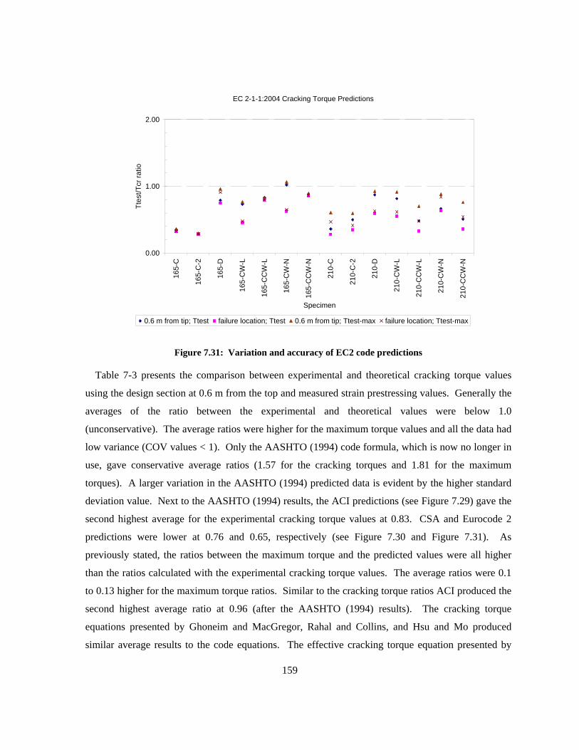
159

EC 2-1-1:2004 Cracking Torque Predictions

0.00

1.00

2.00

165-

C

165-

C-2

165-

D

165-

CW

-L

165-

CC

W-L

165-

CW

-N

165-

CC

W-N

210-

C

210-

C-2

210-

D

210-

CW

-L

210-

CC

W-L

210-

CW

-N

210-

CC

W-N

Specimen

Ttes

t/Tcr

ratio


Figure 7.31: Variation and accuracy of EC2 code predictions

Table 7-3 presents the comparison between experimental and theoretical cracking torque values

using the design section at 0.6 m from the top and measured strain prestressing values. Generally the

averages of the ratio between the experimental and theoretical values were below 1.0

(unconservative). The average ratios were higher for the maximum torque values and all the data had

low variance (COV values < 1). Only the AASHTO (1994) code formula, which is now no longer in

use, gave conservative average ratios (1.57 for the cracking torques and 1.81 for the maximum

torques). A larger variation in the AASHTO (1994) predicted data is evident by the higher standard

deviation value. Next to the AASHTO (1994) results, the ACI predictions (see Figure 7.29) gave the

second highest average for the experimental cracking torque values at 0.83. CSA and Eurocode 2

predictions were lower at 0.76 and 0.65, respectively (see Figure 7.30 and Figure 7.31). As

previously stated, the ratios between the maximum torque and the predicted values were all higher

than the ratios calculated with the experimental cracking torque values. The average ratios were 0.1

to 0.13 higher for the maximum torque ratios. Similar to the cracking torque ratios ACI produced the

second highest average ratio at 0.96 (after the AASHTO (1994) results). The cracking torque

equations presented by Ghoneim and MacGregor, Rahal and Collins, and Hsu and Mo produced

similar average results to the code equations. The effective cracking torque equation presented by

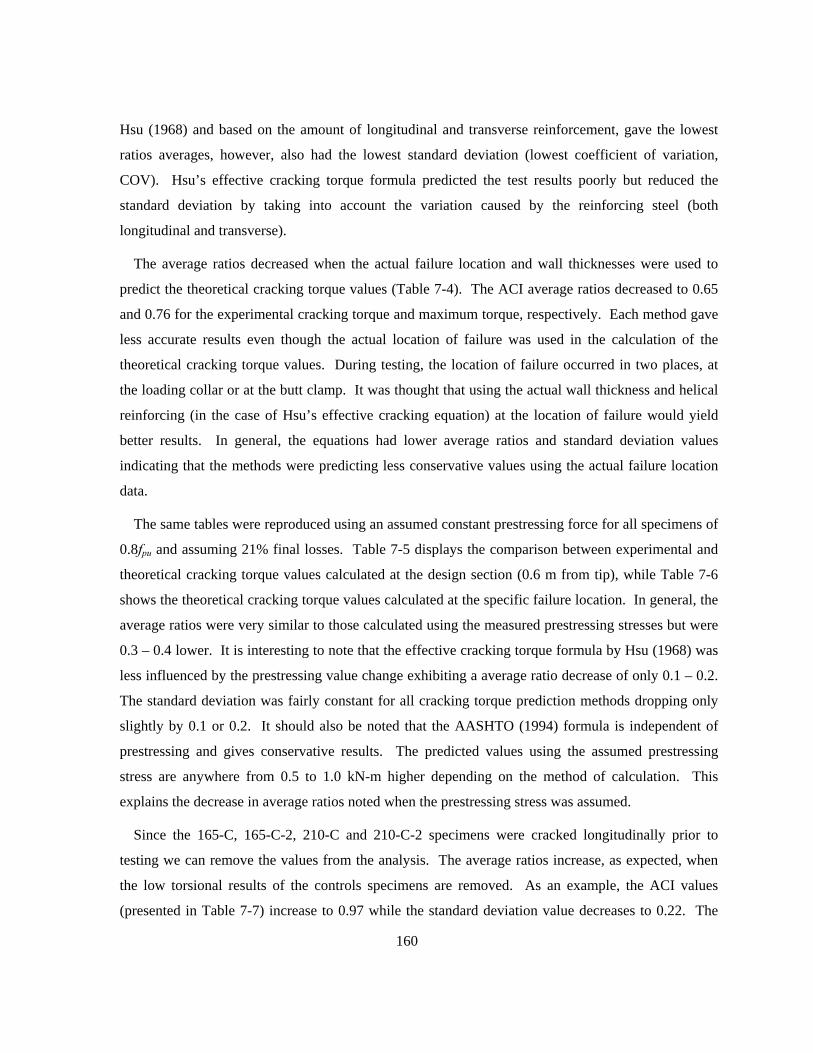
160

Hsu (1968) and based on the amount of longitudinal and transverse reinforcement, gave the lowest

ratios averages, however, also had the lowest standard deviation (lowest coefficient of variation,

COV). Hsu’s effective cracking torque formula predicted the test results poorly but reduced the

standard deviation by taking into account the variation caused by the reinforcing steel (both

longitudinal and transverse).

The average ratios decreased when the actual failure location and wall thicknesses were used to

predict the theoretical cracking torque values (Table 7-4). The ACI average ratios decreased to 0.65

and 0.76 for the experimental cracking torque and maximum torque, respectively. Each method gave

less accurate results even though the actual location of failure was used in the calculation of the

theoretical cracking torque values. During testing, the location of failure occurred in two places, at

the loading collar or at the butt clamp. It was thought that using the actual wall thickness and helical

reinforcing (in the case of Hsu’s effective cracking equation) at the location of failure would yield

better results. In general, the equations had lower average ratios and standard deviation values

indicating that the methods were predicting less conservative values using the actual failure location

data.

The same tables were reproduced using an assumed constant prestressing force for all specimens of

0.8fpu and assuming 21% final losses. Table 7-5 displays the comparison between experimental and

theoretical cracking torque values calculated at the design section (0.6 m from tip), while Table 7-6

shows the theoretical cracking torque values calculated at the specific failure location. In general, the

average ratios were very similar to those calculated using the measured prestressing stresses but were

0.3 – 0.4 lower. It is interesting to note that the effective cracking torque formula by Hsu (1968) was

less influenced by the prestressing value change exhibiting a average ratio decrease of only 0.1 – 0.2.

The standard deviation was fairly constant for all cracking torque prediction methods dropping only

slightly by 0.1 or 0.2. It should also be noted that the AASHTO (1994) formula is independent of

prestressing and gives conservative results. The predicted values using the assumed prestressing

stress are anywhere from 0.5 to 1.0 kN-m higher depending on the method of calculation. This

explains the decrease in average ratios noted when the prestressing stress was assumed.

Since the 165-C, 165-C-2, 210-C and 210-C-2 specimens were cracked longitudinally prior to

testing we can remove the values from the analysis. The average ratios increase, as expected, when

the low torsional results of the controls specimens are removed. As an example, the ACI values

(presented in Table 7-7) increase to 0.97 while the standard deviation value decreases to 0.22. The

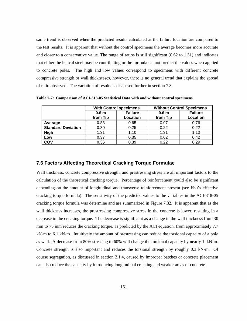
161

same trend is observed when the predicted results calculated at the failure location are compared to

the test results. It is apparent that without the control specimens the average becomes more accurate

and closer to a conservative value. The range of ratios is still significant (0.62 to 1.31) and indicates

that either the helical steel may be contributing or the formula cannot predict the values when applied

to concrete poles. The high and low values correspond to specimens with different concrete

compressive strength or wall thicknesses, however, there is no general trend that explains the spread

of ratio observed. The variation of results is discussed further in section 7.8.

Table 7-7: Comparison of ACI-318-05 Statistical Data with and without control specimens

With Control specimens Without Control Specimens 0.6 m

from Tip Failure

Location 0.6 m

from Tip Failure

Location Average 0.83 0.65 0.97 0.76 Standard Deviation 0.30 0.25 0.22 0.22 High 1.31 1.10 1.31 1.10 Low 0.37 0.35 0.62 0.42 COV 0.36 0.39 0.22 0.29

7.6 Factors Affecting Theoretical Cracking Torque Formulae

Wall thickness, concrete compressive strength, and prestressing stress are all important factors to the

calculation of the theoretical cracking torque. Percentage of reinforcement could also be significant

depending on the amount of longitudinal and transverse reinforcement present (see Hsu’s effective

cracking torque formula). The sensitivity of the predicted values to the variables in the ACI-318-05

cracking torque formula was determine and are summarized in Figure 7.32. It is apparent that as the

wall thickness increases, the prestressing compressive stress in the concrete is lower, resulting in a

decrease in the cracking torque. The decrease is significant as a change in the wall thickness from 30

mm to 75 mm reduces the cracking torque, as predicted by the ACI equation, from approximately 7.7

kN-m to 6.1 kN-m. Intuitively the amount of prestressing can reduce the torsional capacity of a pole

as well. A decrease from 80% stressing to 60% will change the torsional capacity by nearly 1 kN-m.

Concrete strength is also important and reduces the torsional strength by roughly 0.3 kN-m. Of

course segregation, as discussed in section 2.1.4, caused by improper batches or concrete placement

can also reduce the capacity by introducing longitudinal cracking and weaker areas of concrete

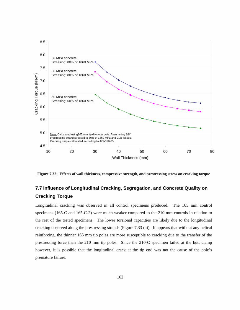
162

4.5

5.0

5.5

6.0

6.5

7.0

7.5

8.0

8.5

10 20 30 40 50 60 70 80Wall Thickness (mm)

Cra

ckin

g To

rque

(kN

-m)

60 MPa concreteStressing: 80% of 1860 MPa

Note: Calculated using165 mm tip diameter pole. Assumming 3/8" prestressing strand stressed to 80% of 1860 MPa and 21% losses.Cracking torque calculated according to ACI-318-05.



Figure 7.32: Effects of wall thickness, compressive strength, and prestressing stress on cracking torque

7.7 Influence of Longitudinal Cracking, Segregation, and Concrete Quality on Cracking Torque

Longitudinal cracking was observed in all control specimens produced. The 165 mm control

specimens (165-C and 165-C-2) were much weaker compared to the 210 mm controls in relation to

the rest of the tested specimens. The lower torsional capacities are likely due to the longitudinal

cracking observed along the prestressing strands (Figure 7.33 (a)). It appears that without any helical

reinforcing, the thinner 165 mm tip poles are more susceptible to cracking due to the transfer of the

prestressing force than the 210 mm tip poles. Since the 210-C specimen failed at the butt clamp

however, it is possible that the longitudinal crack at the tip end was not the cause of the pole’s

premature failure.

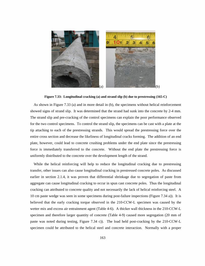
163

(a) (b)

Figure 7.33: Longitudinal cracking (a) and strand slip (b) due to prestressing (165-C)

As shown in Figure 7.33 (a) and in more detail in (b), the specimens without helical reinforcement

showed signs of strand slip. It was determined that the strand had sunk into the concrete by 2-4 mm.

The strand slip and pre-cracking of the control specimens can explain the poor performance observed

for the two control specimens. To control the strand slip, the specimens can be cast with a plate at the

tip attaching to each of the prestressing strands. This would spread the prestressing force over the

entire cross section and decrease the likeliness of longitudinal cracks forming. The addition of an end

plate, however, could lead to concrete crushing problems under the end plate since the prestressing

force is immediately transferred to the concrete. Without the end plate the prestressing force is

uniformly distributed to the concrete over the development length of the strand.

While the helical reinforcing will help to reduce the longitudinal cracking due to prestressing

transfer, other issues can also cause longitudinal cracking in prestressed concrete poles. As discussed

earlier in section 2.1.4, it was proven that differential shrinkage due to segregation of paste from

aggregate can cause longitudinal cracking to occur in spun cast concrete poles. Thus the longitudinal

cracking can attributed to concrete quality and not necessarily the lack of helical reinforcing steel. A

10 cm paste wedge was seen in some specimens during post-failure inspections (Figure 7.34 a)). It is

believed that the early cracking torque observed in the 210-CCW-L specimen was caused by the

wetter mix and excess air entrainment agent (Table 4-6). A thicker wall thickness in the 210-CCW-L

specimen and therefore larger quantity of concrete (Table 4-9) caused more segregation (20 mm of

paste was noted during testing, Figure 7.34 c)). The load held post-cracking by the 210-CCW-L

specimen could be attributed to the helical steel and concrete interaction. Normally with a proper

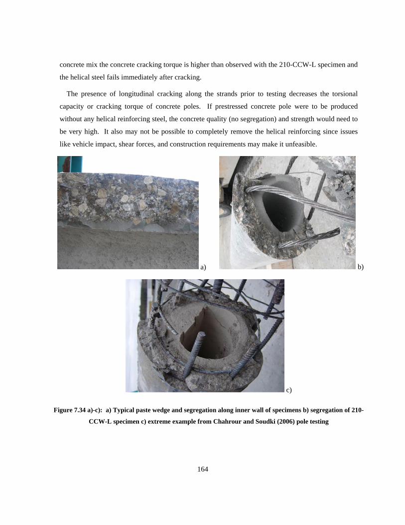
164

concrete mix the concrete cracking torque is higher than observed with the 210-CCW-L specimen and

the helical steel fails immediately after cracking.

The presence of longitudinal cracking along the strands prior to testing decreases the torsional

capacity or cracking torque of concrete poles. If prestressed concrete pole were to be produced

without any helical reinforcing steel, the concrete quality (no segregation) and strength would need to

be very high. It also may not be possible to completely remove the helical reinforcing since issues

like vehicle impact, shear forces, and construction requirements may make it unfeasible.

a) b)

c)

Figure 7.34 a)-c): a) Typical paste wedge and segregation along inner wall of specimens b) segregation of 210-

CCW-L specimen c) extreme example from Chahrour and Soudki (2006) pole testing

165

7.8 Discussion on the Variation in the Results

7.8.1 Sky Cast Inc. Database and Experimental Specimen Comparison

The experimental results discussed in Chapter 6 were compared to a database of test results provided

by Sky Cast Inc. to determine if the specimens were representative of previous findings. The Sky

Cast Inc. database contained many test results ranging from smaller Class A poles to larger Class O

poles. The database provided information on the class, length, helical reinforcement type (single,

double, none), prestressing strand size, wall thickness at failure for bending, and tip diameter.

Specimen specific concrete strengths, wall thickness at torsion failure, and prestressing levels were

not recorded and therefore theoretical calculations were not completed on the database. While the

missing information could have be estimated, the theoretical calculations were not completed since

cracking torque is greatly affected by wall thickness, concrete strength, and prestressing level (as

shown previously in section 7.5 and 7.6).

The database was sorted and plotted into 5 figures with tip diameters of 165 mm and 210 mm and

stressing strand sizes of 3/8”, 7/16” and 1/2”. Poles classified as A through F were used since the

CSA A14-07 standard gives the same spacing and percentage of helical reinforcement as the

experimental specimens tested. The class of a pole relates only to the length and bending capacity of

the pole and does not affect the torsional result as long as wall thickness, tip diameter, and strand

sizes are kept constant. Testing of database single helical reinforcement poles were always completed

in the CCW direction according to the CSA A14-M1979 standard, clause 7.5.4 (torsional load creates

compressive principal stresses along the direction of spirals).

Figure 7.35 plots the database results of 150 mm tip poles with 3/8” prestressing strand. The

results include Class A and B poles and double helix, single helix, and no helical reinforcement. The

single helically reinforced poles results are between 4 and 10 kN-m with the majority between 5 and 8

kN-m. The results of the few double helically reinforced and non reinforced poles tested also fall

between 5 and roughly 8.5 kN-m. The database results suggest that the single helical poles behave

similarly to the double helical and non-reinforced poles. The results also suggest that helical

reinforcement did not increase the torsional capacity of the 150 mm tip poles, and the torsional results

vary between 4 and 9 kN-m regardless of the helical reinforcement type.

166

0

2

4

6

8

10

12

14

Sky Cast Inc. Torsion Database150 mm tip, 3/8" diameter strand

(Class A, and B)

Torq

ue (k

N-m

)

Double Helix Single Helix (CCW) No Helix

Figure 7.35: Sky Cast Inc. Torsion Database Results - 150 mm tip, 3/8" prestressing strand

0

2

4

6

8

10

12

14

Sky Cast Inc. Torsion Database165 mm Tip, 7/16" diameter strand

(Class A, B, C, and D)

Torq

ue (k

N-m

)

Double Helix Single Helix (CCW) No Helix


167

The database also contained 165 mm tip poles with stressing strands sizes of 3/8”, 7/16”, and 1/2”.

The majority of the poles tested used 7/16” strand (Figure 7.36). Similar to the 150 mm tip pole

results, the 165 mm tip poles with 7/16” strand lie within a band of roughly 5 to 10 kN-m with a few

outliers. Again, no significant difference in torsional capacity was observed between the double

helical poles and the single/no helix poles. The results indicate further that the helical reinforcement

does not contribute significantly to the torsional capacity of the pole tested. The variation in the

torsional capacities (5 to 10 kN-m) is slightly higher, but very similar to the band determined from the

150 mm tip poles (4 to 9 kN-m). The similar results can be explained by the concrete area difference

between a 150 mm tip pole and 165 mm tip pole being small. It should be noted that the prestressing

strand size, while doubled from 3/8” to 7/16” strand, increased the torsional capacity only slightly.

Figure 7.37 shows the 165 mm tip poles tested with 1/2” prestressing strand. Similarly to Figure

7.35 and Figure 7.36, the double helix and single helix specimens do not show a difference in

torsional capacity and all the results lie within a band of 6 – 9 kN-m. Again, similar to the 165 mm

tip - 7/16” strand results, it appears that the prestressing strand size does not affect the torsional

capacity very much. Failure of the specimens may be caused by some other phenomenon and as a

result the increased strand size does not cause a noticeable increase in the torsional capacity.

To determine if the experimental results were in agreement with the Sky Cast Inc. database results,

poles with the same tip diameter as the 14 experimental specimens were selected and plotted together

with the experimental results (Figure 7.38 and Figure 7.39). Due to the lack of results to compare to

the 210 mm specimens with 3/8”, 7/16”, and 1/2” strands were plotted together with the 210

experimental specimens since it was determined in the previous figures that prestressing strand size

does seem to affect the torsional capacity of the pole to a great extent.

The 165 mm tip experimental specimens all behaved similarly to the database results (Figure 7.38).

While the 165-D specimen had a lower torsional capacity than the database results, the specimen still

fell within the 6 to 10 kN-m band observed. According to the database results the double helix does

not seem to hold more torsional load than the single/non-reinforced specimens. The 165-CCW-N and

165-CW-N specimens were found to lie in the middle of the database results as expected since the

single helix (CCW) poles were reinforced and tested in the same manner. Even though the engaged

reinforcing direction (CW) yielded larger torsional capacities in the experimental testing, the database

results (tested in the CCW direction) do not support this result.

168

0

2

4

6

8

10

12

14


(Class B, E, and F)

Torq

ue (k

N-m

)

Double Helix Single Helix (CCW)


165-C 165-C-2

165-D165-CW-L 165-CCW-L

165-CW-N

165-CCW-N

0

2

4

6

8

10

12

14


(Class A, B, C, and D)

Torq

ue (k

N-m

)


Experimental SpecimensNote: Experimental specimens contained 3/8" strand.

Figure 7.38: Sky Cast Inc. Torsion Database and Experimental Results - 165 mm tip, 3/8"strand

169

The database had several poles, tested in the CCW direction, which gave larger torsional results

than the 165-CW-N specimen. This fact seems to suggest that the direction of the reinforcement does

not affect the capacity of the pole. The large spaced, non CSA A14-07 conforming poles, 165-CW-L

and 165-CCW-L, interestingly enough also behaved similar to the low end single helix results from

the database. This suggests that the spacing of the helical reinforcement is also insignificant to the

overall variation observed in the database. The non reinforced experimental specimens (165-C and

165-C-2) behaved significantly below the other database results. While no non-helical reinforced

specimens were tested with 3/8” strand in the database, previous figures suggest that the non-

reinforced specimens typically lie within the band 5 – 10 kN-m band. The poor performance of the

165-C and 165-C-2 specimens can likely be linked to the longitudinal cracking observed. Concrete

strength and wall thickness differences may also have contributed.

Since there are fewer Sky Cast Inc. database results for the 210 mm tip poles, less can be

conclusively derived. The 210 mm tip experimental specimens are compared with 10 poles from the

database in Figure 7.39. While one of the non-reinforced specimens (210-C-2) was in the middle of

the database results, the other specimen (210-C) was lower than all the other database results. The

low result observed by the 210-C specimen is still within 2 kN-m of the other results and could seem

further removed due to the lower number of results available for comparison. The 210-CCW-L, 210-

CCW-N, and 210-CW-N specimens all were relatively close to the database results. The results

further the suggestion presented in the 165 mm tip data that the spacing of the helical reinforcement

does not affect the torsional capacity. However, the 210-D, 210-CW-L and 210-CW-N poles appear

to have increased torsional capacity compared to the database results. This result suggests that the

direction may have an influence on the larger sized poles or that not enough database results are

available for comparison and the band of results is actually wider. The increased capacity exhibited

by the 210-D and 210-CW-L may be due to differences in concrete and is unlikely related to the

helical reinforcement as the specimens with more helical reinforcement actually exhibited smaller

torsional capacities.

Without further testing the observations made can not be conclusively stated, however from the

experimental results both differences in wall thickness and concrete strength can not explain the

increase in torsional capacities observed. It is apparent that helical steel affects the cracking torque of

the specimen, however the mechanism and how much the steel contributes is unknown.

170

210-C

210-C-2

210-D

210-CW-L

210-CCW-L

210-CW-N

210-CCW-N

0

2

4

6

8

10

12

14

Sky Cast Inc. Torsion Database210 mm Tip, 3/8", 7/16", 1/2" diameter strand

(Class C, D, E, and F)

Torq

ue (k

N-m

)


No Helix Experimental SpecimensNote: Experimental specimens contained 3/8" strand.

Figure 7.39: Sky Cast Inc. Torsion Database and Experimental Results - 210 mm tip

7.8.2 Experimental Variation and the CSA A14-07 Spacing Provisions

Of the seven 165 mm poles tested, only three were acceptable according to current CSA A14-07

standards (165-D, 165-CW-N, and 165-CCW-N). The remaining poles were not designed based on

CSA A14-07; 165-C and 165-C-2 contained no reinforcing and the spacing was too large for the 165-

CW-L and 165-CCW-L specimens. The variation and scatter observed during testing of the

specimens and in the Sky Cast Inc. database results could be explained by insufficient transfer zone

helical steel.

The three specimens designed based on the code displayed similar behaviour after cracking, adding

approximately 0.5 to 1.5 kN-m to the torque sustained in post-cracking region (Figure 7.40). The

cracking torques ranged from 6.7 to 8.5 kN-m for the 165-D and 165-CW-N specimens respectively.

The remaining poles, excluding the control specimens, exhibited cracking torques of 6.1 and 5.9 kN-

m and held the cracking torque or maintained no additional post-crack torque (Figure 7.41). The

results suggest that for the 165 mm specimens the code designed poles have a better ability to

maintain the cracking torque in the post-cracking region and have larger cracking torques in general.

171

0

2

4

6

8

10

0 0.002 0.004 0.006 0.008 0.01twist (rad/m)

Torq

ue (k

N-m

)

165-D 165-CW-N 165-CCW-N

165-D

165-CCW-N

165-CW-N

Figure 7.40: 165 mm specimens designed to CSA A14

0

2

4

6

8

10

0 0.002 0.004 0.006 0.008 0.01twist (rad/m)

Torq

ue (k

N-m

)

165-C 165-C-2 165-CW-L 165-CCW-L

165-C

165-CCW-L

165-CW-L

165-C-2

Figure 7.41: 165 mm specimens against CSA A14

0

2

4

6

8

10

12

14

0 0.002 0.004 0.006 0.008 0.01twist (rad/m)

Torq

ue (k

N-m

)

210-D 210-CW-N 210-CCW-N

210-D

210-CCW-N

210-CW-N

Figure 7.42: 210 mm specimens designed to CSA A14

0

2

4

6

8

10

12

14

0 0.002 0.004 0.006 0.008 0.01twist (rad/m)

Torq

ue (k

N-m

)

210-C 210-C-2 210-CW-L 210-CCW-L

210-C

210-C-2

210-CW-L

210-CCW-L

Figure 7.43: 210 mm specimens against CSA A14

However, the difference between the highest cracking torque for the non-code designed poles (165-

CW-L) and the lowest cracking torque for the code designed poles (165-D) is only 0.6 kN-m.

The 210 mm specimens behaved differently than the 165 mm specimens. Two of the code

allowable poles (210-D and 210-CW-N) displayed similar ultimate torque values of 12 kN-m. Both

normal spaced specimens (210-CW-N and 210-CCW-N) however cracked 3 kN-m below the 210-D

specimen. In fact, the 210-CW-L exhibited a larger cracking torque value indicating that the code

designed poles may in fact not be better than the non-code designed poles. However, it cannot be

conclusively stated since the 210-CCW-L specimen cracked much lower than all the specimens.

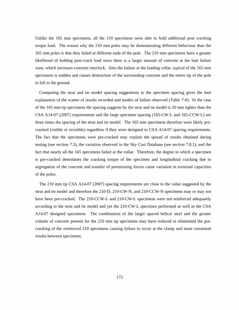
172

Unlike the 165 mm specimens, all the 210 specimens were able to hold additional post cracking

torque load. The reason why the 210 mm poles may be demonstrating different behaviour than the

165 mm poles is that they failed at different ends of the pole. The 210 mm specimens have a greater

likelihood of holding post-crack load since there is a larger amount of concrete at the butt failure

zone, which increases concrete interlock. Also the failure at the loading collar, typical of the 165 mm

specimens is sudden and causes destruction of the surrounding concrete and the entire tip of the pole

to fall to the ground.

Comparing the strut and tie model spacing suggestions to the specimen spacing gives the best

explanation of the scatter of results recorded and modes of failure observed (Table 7-8). In the case

of the 165 mm tip specimens the spacing suggests by the strut and tie model is 20 mm tighter than the

CSA A14-07 (2007) requirements and the large specimen spacing (165-CW-L and 165-CCW-L) are

three times the spacing of the strut and tie model. The 165 mm specimens therefore were likely pre-

cracked (visible or invisible) regardless if they were designed to CSA A14-07 spacing requirements.

The fact that the specimens were pre-cracked may explain the spread of results obtained during

testing (see section 7.5), the variation observed in the Sky Cast Database (see section 7.8.1), and the

fact that nearly all the 165 specimens failed at the collar. Therefore, the degree to which a specimen

is pre-cracked determines the cracking torque of the specimen and longitudinal cracking due to

segregation of the concrete and transfer of prestressing forces cause variation in torsional capacities

of the poles.

The 210 mm tip CSA A14-07 (2007) spacing requirements are close to the value suggested by the

strut and tie model and therefore the 210-D, 210-CW-N, and 210-CCW-N specimens may or may not

have been pre-cracked. The 210-CCW-L and 210-CW-L specimens were not reinforced adequately

according to the strut and tie model and yet the 210-CW-L specimen performed as well as the CSA

A14-07 designed specimens. The combination of the larger spaced helical steel and the greater

volume of concrete present for the 210 mm tip specimens may have reduced or eliminated the pre-

cracking of the reinforced 210 specimens causing failure to occur at the clamp and more consistent

results between specimens.

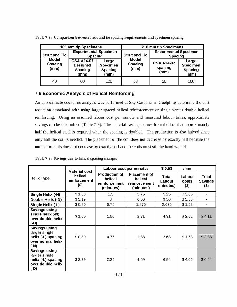
173

Table 7-8: Comparison between strut and tie spacing requirements and specimen spacing

165 mm tip Specimens 210 mm tip Specimens Experimental Specimen

Spacing Experimental Specimen

Spacing Strut and Tie Model

Spacing (mm)

CSA A14-07 Designed Spacing

(mm)

Large Specimen Spacing

(mm)

Strut and Tie Model

Spacing (mm)

CSA A14-07 spacing

(mm)

Large Specimen Spacing

(mm)

40 60 120 53 50 100

7.9 Economic Analysis of Helical Reinforcing

An approximate economic analysis was performed at Sky Cast Inc. in Guelph to determine the cost

reduction associated with using larger spaced helical reinforcement or single versus double helical

reinforcing. Using an assumed labour cost per minute and measured labour times, approximate

savings can be determined (Table 7-9). The material savings comes from the fact that approximately

half the helical steel is required when the spacing is doubled. The production is also halved since

only half the coil is needed. The placement of the coil does not decrease by exactly half because the

number of coils does not decrease by exactly half and the coils must still be hand wound.

Table 7-9: Savings due to helical spacing changes

Labour cost per minute: $ 0.58 /min

Helix Type Material cost

helical reinforcement

($)

Production of helical

reinforcement (minutes)

Placement of helical

reinforcement (minutes)

Total Labour

(minutes)

Labour costs

($)

Total Savings

($)

Single Helix (-N) $ 1.60 1.5 3.75 5.25 $ 3.06 - Double Helix (-D) $ 3.19 3 6.56 9.56 $ 5.58 - Single Helix (-L) $ 0.80 0.75 1.875 2.625 $ 1.53 - Savings using single helix (-N) over double helix (-D)

$ 1.60 1.50 2.81 4.31 $ 2.52 $ 4.11

Savings using larger single helix (-L) spacing over normal helix (-N)

$ 0.80 0.75 1.88 2.63 $ 1.53 $ 2.33

Savings using larger single helix (-L) spacing over double helix (-D)

$ 2.39 2.25 4.69 6.94 $ 4.05 $ 6.44

174

It can be approximated that $2.33 can be saved per pole using the larger spaced single helical

spacing (-L). Using a similar method, approximately $4.11 can be saved using the single helix (-N)

over the double helix (-D). When the single helix at the large spacing is compared against the double

helix spacing we get a total savings of approximately $6.44. The savings may not be significant when

it is compared to the $300 total production cost of a single pole. When large volumes of poles are

produced, savings may be more substantial.

7.10 Analysis and Comparison of Typical Applied Torques on Lighting Poles

Typical applied loads on lighting poles were calculated to determine if the torque capacity of the

tested poles was adequate. A standard cobra head fixture with an Effective Projected Area (EPA) of

0.093 m2 (1 ft2) and a fixture arm length of 2.4 m (8 ft) and EPA of 0.055 m2 (0.6 ft2) were used to

calculated wind torque loads due to 80 and 160 mph wind speeds using the AASHTO LTS-4-M

(2001) static wind pressure formula below:

drZ CIGVKP 2613.0= (7-3)

where KZ is a height and exposure factor, G is the gust effect factor of 1.14, V is the design wind

velocity in mph, Ir is a wind importance factor, Cd is the drag coefficient, and P is the static wind

pressure in Pa. Appendix E contains the product sheets showing where the EPA values were taken

from and a print out of the wind load calculation spreadsheet.

Calculating the height and exposure factor for 10.7 m gave a value of 1.09. The gust factor was

calculated to be 1.14. Since the poles were near 10 m in height, the wind importance factor was taken

as 1. A drag coefficient of 1 was used since the EPA values given by the manufacturers already

incorporate the fixture’s drag coefficient. The 80 mph wind speed was considered as a design wind

speed for non-hurricane regions (Waterloo, Ontario) whereas the 160 mph wind speed was assumed

for hurricane regions. The factored calculated values of applied torque for the 80 mph and 160 mph

wind speeds were calculated as 0.4 kN-m, and 1.84 kN-m respectively.

The ACI (Clause 11.6.1) and CSA (Clause 11.2.9.1) code indicate that if the factored torsional

loads are below 0.25Tcr than the torsional loads can be ignored for design. The clauses in both codes

can be linked to a report by ACI Committee 438 (1969). The report suggests that torsion can be

neglected in design if the nominal ultimate stress due to torsion is less than '5.1 cfφ . The stress

suggested is approximately 25 percent of the pure torsional strength of a member without web

175

reinforcement. The simplification for design is considered allowable since a torsional moment

applying a stress of '5.1 cfφ will not cause a significant reduction in ultimate strength in flexure of

shear. In beams without stirrups, a torsional moment of 30 percent of the pure torsional strength

causes no reduction in the flexural strength, and reduces the shear strength by about 5-15 percent. It

is suggested that the reduction in shear strength can be compensated by the post-cracking shear

strength, since shear strength is based on diagonal cracking and is less than the actual ultimate shear

strength. Beams with stirrups the stress corresponds to a torsional moment much less than 25 percent

of the pure torsional strength. The flexural strength is reduced by a few percent only and shear

strength is reduced by about 15 percent.

The associated factored resistance (calculated using CSA cracking torque equations and including

factors of safety (φc = 0.7)) for the lowest 165 mm tip diameter specimen can be calculated as 5.18

kN-m and 9.29 kN-m for the 210 mm specimen. The 0.25Tcr values are 1.3 kN-m and 2.3 kN-m

respectively. This indicates that even the lowest strength specimen could have been designed

neglecting torsion in non-hurricane areas. Only in the 210 mm lighting pole specimens however, can

the torsional forces be neglected in hurricane areas (Figure 7.44 and Figure 7.45).

In hurricane areas torsion effects must be considered in addition to bending and shear, however the

torsional loads are still well below the tested cracking torque values. The specimens have adequate

reserve strength for torsional loads however the torsional loads above 0.25Tc may cause a reduction in

the shear or moment capacities. For torsional resistance, poles have better geometry and control of

material properties than beams cast on site and since the design recommendation of 0.25Tcr was

developed for structural beam elements, it is likely too conservative for concrete lighting poles. It

should be noted that the difference between the cracking torques of the CSA A14-07 acceptable and

unacceptable specimens is insignificant when compared to the torques typically applied to street

lighting poles. As a result, the spacing of the helical reinforcement is insignificant compared to the

applied torques and the CSA A14-07 requirements can likely be simplified.

176

0.7(0.25 Tcr)Tf (160 mph)

Tf (80 mph)0

1

2

3

4

5

6

7

8

9

10

0 0.001 0.002 0.003 0.004 0.005 0.006 0.007 0.008 0.009 0.01twist (rad/m)

Torq

ue (k

N-m

)

165-D 165-C 165-C-2 165-CW-L 165-CCW-L 165-CW-N 165-CCW-N

Figure 7.44: Applied factored torque versus 165 cracking torques

0.7(0.25 Tcr)Tf (160 mph)

Tf (80 mph)0

2

4

6

8

10

12

14

0 0.002 0.004 0.006 0.008 0.01twist (rad/m)

Torq

ue (k

N-m

)

210-D 210-C 210-C-2 210-CW-L 210-CCW-L 210-CW-N 210-CCW-N

Figure 7.45: Applied factored torque versus 210 cracking torques

177

Chapter 8 Conclusions and Recommendations for Future Work

An investigation into the effect of helical reinforcement on the torsional capacity of prestressed

concrete poles was completed. The objectives of the investigation were to analyze the Canadian code

(CSA A14-07) and compare the minimum helical reinforcing requirements to other concrete pole

codes. Spacing requirements and direction of the helical steel reinforcing effects on torsional

capacity were determined and double and single helix reinforcement methods analyzed. The mode of

failure and post-cracking behaviour were also presented and analyzed. The reason for inclusion of

helical reinforcement in prestressed concrete poles and the main factors influencing the torsional

capacity of prestressed concrete poles were determined. The investigation yielded the conclusions

and results.

• The response of the poles could be modelled closely using a linear elastic torsion model,

suggesting that the failure is at the cracking torque of the concrete. The model was

dependent on the assumed modulus of elasticity and wall thickness. The torsional failure

mode for concrete poles is brittle and sudden with no post-cracking ductility provided by

the helical reinforcing steel. It appears that the added torsional capacity from the helical

reinforcement is insignificant when compared to the torsional capacity contributed by the

concrete.

• The helical reinforcing may influence the cracking torque capacity of the prestressed

concrete pole. The helical steel provides some confinement to the inner concrete and also

intercepts cracks and increases the cracking torque.

• Little difference in torsional capacity was observed between the clockwise (CW; engaged

helical steel) and counter clockwise (CCW) helically reinforced specimens. For the

smaller 165 mm tip specimens, the CW specimens had slightly higher cracking torque

values. The trend was not observed with the 210 mm specimens. The helix direction was

determined to be insignificant to the torsional capacity of the concrete pole.

• Spacing of the helical reinforcement as suggested by the CSA A14-07 code and twice the

code spacing had little effect on the torsional capacity of the pole. Higher results were

noted with 165 mm specimens when tighter spaced helical reinforcement was used.

178

• Quality assurance of the concrete, prestressing levels and wall thickness are all important

factors for the torsional capacity of prestressed concrete poles. Segregation caused by poor

concrete, low concrete strengths, and insufficient reinforcement for the transfer of

prestressing loads cause longitudinal cracks to develop, which reduce the torsional capacity

of the pole.

• The Compression Field Theory was found to better predict the post-cracking region of the

concrete pole test results than the Softened Truss Model. For prestressed concrete poles it

is apparent that the cover spalls and post-cracking loads are sustained by the helical

reinforcement and interlock of the concrete.

• The pole cracking torque was best predicted by the ACI-318-05 code. CSA A23.3-04 and

Eurocode 2 were less conservative than ACI. All codes predicted unconservative results

on average and a large scatter in the predicted results was noted. The database of previous

torsional tests had results scattered over a range of 5 to 10 kN-m regardless of the direction

and method of helical reinforcement.

• Strut and tie modeling of the transfer zone determined that a 40 mm helical reinforcement

spacing was needed for the 165 mm specimens in the first 500 mm from the tip. The 210

mm specimens required a 53 mm spacing in the prestressing transfer zone. CSA, ACI, and

EC2 code determined maximum spacing of the minimum transverse reinforcement was

between 47 – 62 mm for the 165 specimens and 40 – 49 mm for the 210 mm specimens.

The strut and tie model and code spacing requirements indicate that all the 165 mm

specimens and the large spaced 210 mm specimens (210-CW-L and 210-CCW-L) were

insufficiently reinforced in the transfer zone. The insufficient reinforcement may explain

the scatter of results observed during tested since the specimens could have been pre-

cracked to different degrees.

• Torsional loads are typically not a governing factor in the design of concrete lighting poles.

In the case of the 165 mm and 210 mm tip specimens the applied loads due to a standard

fixture gave negligible or near negligible loads.

Potential exists for the simplification of the CSA A14-07 code in regards to minimum reinforcing

requirements and torsional capacities. It is suggested that the requirements be modelled similar to the

American (ASTM C 1089-06) requirements. A spacing of 30 mm to 50 mm is recommended in the

179

transfer zone (approximately 50 times the strand diameter) depending on the pole tip size. The

American limit of 102 mm in the remaining portions of the pole requires further investigation. Proper

spun cast concrete mixes and adequate concrete strengths, prestressing levels, and wall thickness all

have a large impact on the torsional capacity of prestressed concrete poles and therefore should be

emphasized in the CSA A14-07 design requirements.

It is recommended that an extensive testing program be undertaken to conclusively determine if

direction and spacing have an effect on torsional capacity or to ultimately determine the factors

causing the scatter in the results. Further torsional and helical reinforcement research should

investigate the performance of prestressed concrete poles reinforced using the suggestions based on

the strut and tie model results. If more torsional tests are performed on concrete poles, a method to

entirely eliminate the flexural load other than the use of a restraining cable would be beneficial.

Reducing the scatter of the results and providing conservative predictions of the cracking torque of

prestressed concrete poles is desirable to provide safe, rationale concrete pole designs. A better

understanding of the factors that influence the cracking torque in reinforced and prestressed concrete

will allow for safer and more economical designs to be produced.

180

References

AASHTO LTS-3 (1994), “Standard Specification for Structural Supports for Highway Signs,

Luminaries and Traffic Signals”, American Association of State Highway and Transportation

Officials, Washington, D.C., U.S.A, 1994.

AASHTO LTS-4-M, “Standard Specification for Structural Supports for Highway Signs, Luminaries

and Traffic Signals”, American Association of State Highway and Transportation Officials,

Washington, D.C., U.S.A, 2001.

ACI Committee 318, “Building Code Requirements for Structural Concrete and Commentary (ACI

318-05)”, American Concrete Institute, Farmington Hills, Detroit, Michigan, U.S.A, 2005.

ACI Committee 438, “Tentative Recommendations for the Design of Reinforced Concrete Members

to Resist Torsion”, ACI Journal, January 1969, 8 pp.

ACI Committee 445, State of the Art Report: Design for Torsion in Concrete Structures - Draft Copy,

American Concrete Institute, Detroit, 2006, 173 pp.

Ali, M.A., and White, R.N., “Toward a Rational Approach for Design of Minimum Torsion

Reinforcement”, ACI Structural Journal, Vol. 96, No. 1, January-February, 1999, pp. 40-46.

ASCE Concrete Pole Task Committee, Guide for the Design and Use of Concrete Poles, American

Society of Civil Engineers, New York, 1987, 52 pp.

ASCE-PCI Committee Report, “Guide for the Design of Prestressed Concrete Poles”, PCI Journal,

November-December 1997, Vol. 42. No. 6, pp. 93-134.

ASTM C 1089-06, “Standard Specification for Spun Cast Prestressed Concrete Poles”, ASTM

International, West Conshohocken, PA., U.S.A, 2006.

ASTM C 1089-97, “Standard Specification for Spun Cast Prestressed Concrete Poles”, ASTM

International, West Conshohocken, PA., U.S.A, 1997.

Bolander, J., Sowlat, K., and Naaman, A.E., “Design Considerations for Tapered Prestressed

Concrete Poles”, PCI Journal, Vol. 33, No. 1, January-February, 1988, pp. 44-66.

Rosson, B.T., Rohde, J.R., and Klovsky, R., “Behaviour and Design of Static Cast Prestressed

Concrete Distribution Poles”, PCI Journal, Vol. 41, No. 5, September-October, 1996, pp. 94-107.

181

CAN/CSA-S6-06, “Canadian Highway Bridge Design Code (CHBDC)”, Canadian Standards

Association International, Mississauga, Ontario, Canada, 2006.

CSA A14-M1979, “Concrete Poles”, Canadian Standards Association International, Mississauga,

Ontario, Canada, 1979.

CSA A14-00, “Concrete Poles”, Canadian Standards Association International, Mississauga, Ontario,

Canada, 2000.

CSA A14-07, “Concrete Poles”, Canadian Standards Association International, Mississauga, Ontario,

Canada, 2007.

Chahrour, A.H., and Soudki, K.A., “Structural Retrofitting of Deteriorated Concrete Lighting Poles

Using FRP Sheets in Wet Layup – Field Application”, Journal of Composites for Construction,

ASCE, May-June, 2006, pp 234-243.

Collins, M.P. and Mitchell, D., “Shear and Torsion Design of Prestressed and Non-Prestressed

Concrete Beams”, Journal of the Prestressed Concrete Institute, Vol. 25, No. 5, September-

October, 1980, pp. 32-100.

CSA A23.3-04, “Design of Concrete Structures”, Canadian Standards Association International,

Mississauga, Ontario, Canada, 2004.

DIN 1045, “Tragwerke aus Beton, Stahlbeton und Spannbeton – Teil 1: Bemessung und Konstruktion

(Concrete, reinforced and prestressed concrete structures – Part 1: Design)”, DIN 1045-1:2001-07,

Deutsche Institut für Normung e.V., Berlin, Germany, June 2001.

DIN EN 12843, “ Betonfertigteile – Maste (Precast Concrete Products –Masts and Poles)”, DIN EN

12843:2004, Deutsche Institut für Normung e.V., Berlin, Germany, 2004.

DIN EN 40-4, “Lichtmaste – Teil 4: Anforderungen an Lichtmaste aus Stahl- und Spannbeton

(Lighting columns - Part 4: Requirements for reinforced and prestressed concrete lighting

columns)”, DIN EN 40-4:2005, Deutsche Institut für Normung e.V., Berlin, Germany, June 2006.

DIN 4228, “Werkmäßig hergestellte Betonmaste”, Deutsche Institut für Normung e.V., Berlin,

Germany, February 1989.

Dilger, W.H., and Ghali, A., “Response of Spun Cast Concrete Poles to Vehicle Impact”, PCI

Journal, Vol. 31, No. 1, January-February, 1986, pp. 62-82.

182

Dilger, W.H., Ghali, A., and Rao, S.V.K.M., “Improving the Durability and Performance of Spun-

Cast Concrete Poles”, PCI Journal, Vol. 41, No. 2, March-April, 1996, pp. 68-90.

Dilger, W.H., and Rao, S.V.K.M., “High Performance Concrete Mixtures for Spun-Cast Concrete

Poles”, PCI Journal, Vol. 42, No. 2, July-August, 1997, pp. 82-96.

EN 1992-1-1:2004, “Eurocode 2: Design of Concrete Structures – Part 1-1: General rules and rules

for buildings”, BS EN 1992-1-1:2004, British Standards Institution, December 2004.

Fouad, F.H., Scott, N.L., Calvert, E., and Donovan, M., “Performance of Spun Prestressed Concrete

Poles During Hurricane Andrew”, PCI Journal, Vol. 39, No. 2, March-April, 1994, pp. 102-110.

Fouad, F.H., Sherman, D, and Werner, R.J., “Spun Prestressed Concrete Poles – Past, Present, and

Future”, Concrete International, Vol. 14 No. 11, November 1992, pp. 25-29.

Ghoneim, M.G., and MacGregor, J.G., “Evaluation of Design Procedures for Torsion in Reinforced

and Prestressed Concrete”, Report No. 184, Department of Civil Engineering, University of

Alberta, Edmonton, February 1993, 301 pp.

Hsu, T. T. C., “Torsion of Structural Concrete – A Summary on Pure Torsion”, Torsion of Structural

Concrete, Special Publication No. 18-6, American Concrete Institute, Detroit, 1968.

Hsu, T. T. C., Torsion of Reinforced Concrete, Van Nostrand Reinhold, Inc., New York, 1984, 544

pp.

Hsu, T. T. C. and Mo, Y.L., “Softening of Concrete in Torsional Members – Prestressed Concrete”,

ACI Journal, Vol. 82, No. 5, September-October, 1985, pp. 603-615.

Hsu, T. T. C., “Softened Truss Model Theory for Shear and Torsion”, Structural Journal of the

American Concrete Institute, Vol. 85, No. 6, November–December, 1988, pp. 624-635.

Hsu, T. T. C. and Zhang, L. X., “Nonlinear Analysis of Membrane Elements by Fixed-Angle

Softened-Truss Model”, ACI Structural Journal, Vol. 94, No. 5, 1997, pp. 483-492.

Kaufmann, J.P., Hesselbarth, D., Moser, K., and Terrasi, G.P., “Application of fiber reinforced high

performance composites in spun-cast elements”, Materials and Structures, V. 38 No. 279, June,

2005, pp. 549-555.

183

Koutchoukali, N. and Belarbi, A., “Torsion of High-Strength Reinforced Concrete Beams and

Minimum Reinforcement Requirement”, ACI Structural Journal, Vol. 98, No. 4, July-August,

2001, pp. 658-666.

MagGregor, J.G., and Ghoneim, M.G., “Design for Torsion”, ACI Journal, Vol. 92, No. 2, March-

April, 1995, pp. 211-218.

McMullen, A.E. and El-Degwy, W.M., “Prestressed Concrete Tests Compared With Torsion

Theories”, PCI Journal, Vol. 35, No. 5, September-October, 1985, pp. 96-127.

Mitchell, D., and Collins, M.P., “Diagonal Compression Field Theory – A Rational Model for

Structural Concrete in Pure Torsion”, ACI Journal, Vol. 71, August 1974, pp. 396-408.

PCI Committee on Prestressed Concrete Poles, “Guide Specification for Prestressed Concrete Poles”,

PCI Journal, Vol. 27, No 3. May-June, 1982, 13 pp.

PCI Committee on Prestressed Concrete Poles, “Guide for the Design of Prestressed Concrete Poles”,

PCI Journal, Vol. 28, No. 3, May-June 1983, 67 pp.

Rahal, K. N., “Torsional Strength of Reinforced Concrete Beams”, Canadian Journal of Civil

Engineering, Vol. 27, No. 3, 2000, pp. 445–453.

Rahal, K.N. and Collins, M.P., “Simple Model for Predicting Torsional Strength of Reinforced and

Prestressed Concrete Sections”, ACI Structural Journal, Vol. 93, No. 6, November-December,

1996, pp. 658-666.

Rodgers, T.E., “Prestressed Concrete Poles – State of the Art”, PCI Journal, Vol. 29, No. 4,

September-October 1984, 53 pp.

Smith, P., “Impact Testing of Lighting Poles and Sign Supports, 1967-1968”, Report RR158,

Department of Highways Ontario Canada, March, 1970, 33 pp.

Terrasi, G.P., Battig, G., and Bronnimann, R., “Pylons made of high-strength spun concrete and

prestressed with carbon fiber reinforced plastic for high power transmission lines”, International

Journal of Materials and Product Technology, Vol. 17 No. 1-2, 2002, pp. 32-45.

Terrasi, G.P., and Lees, J.M., “CFRP Prestressed Concrete Lighting Columns”, Special Publication

No. 215-3, American Concrete Institute, 2003, pp. 55-74.

184

Wang, M., Dilger, W., and Kuebler, U., “High Performance Concrete for Spun-Cast Utilities Poles”,

Proceedings of the 2001 Second International Conference on Engineering Materials Volume 2,

Canadian Society of Civil Engineers and Japan Society of Civil Engineers, August 2001, pp. 143 -

154.

185

Appendix A Pole Analysis Output for Design of Specimen

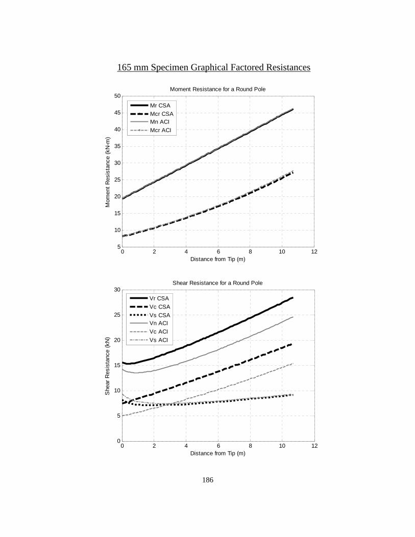
186

165 mm Specimen Graphical Factored Resistances

0 2 4 6 8 10 125

10

15

20

25

30

35

40

45

50


Mom

ent R

esis

tanc

e (k

N-m

)



0 2 4 6 8 10 120

5

10

15

20

25

30


She

ar R

esis

tanc

e (k

N)



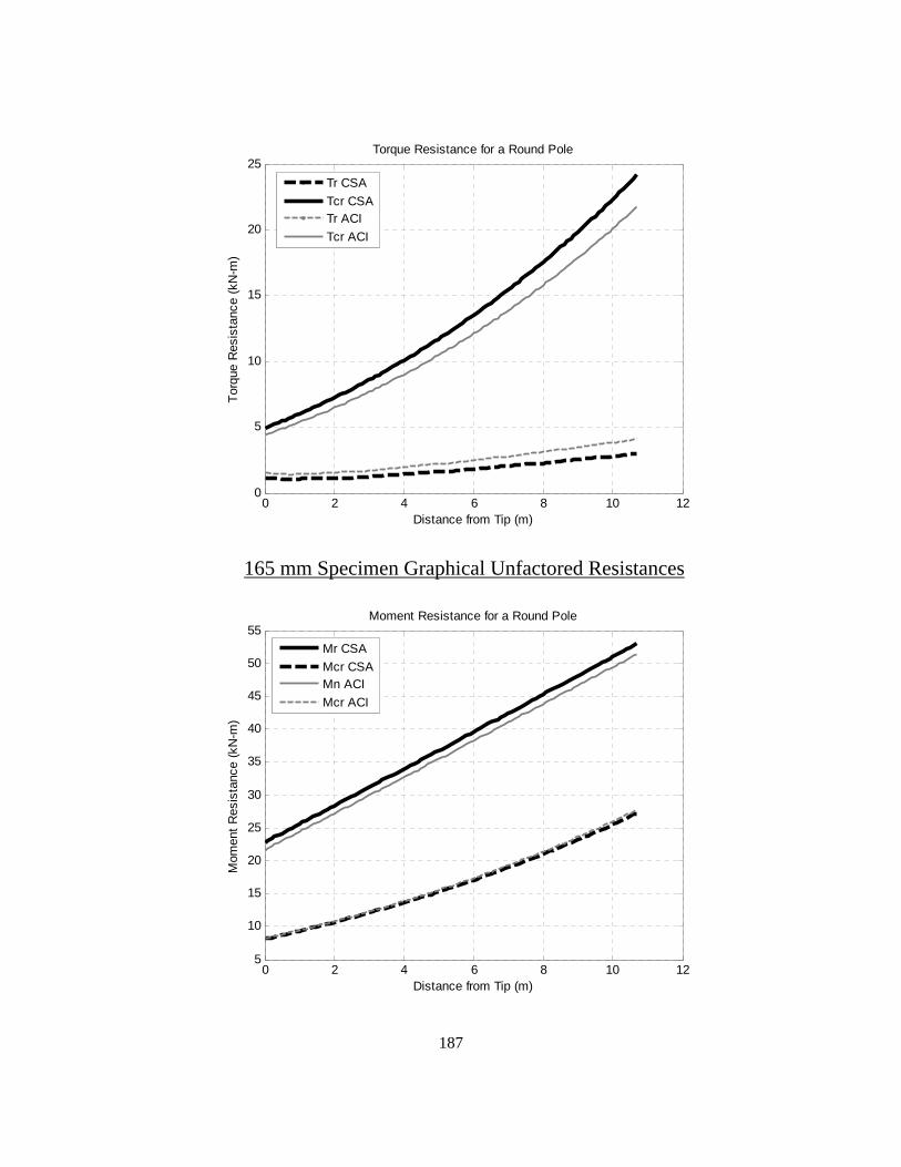
187

0 2 4 6 8 10 120

5

10

15

20

25


Torq

ue R

esis

tanc

e (k

N-m

)



165 mm Specimen Graphical Unfactored Resistances

0 2 4 6 8 10 125

10

15

20

25

30

35

40

45

50

55


Mom

ent R

esis

tanc

e (k

N-m

)



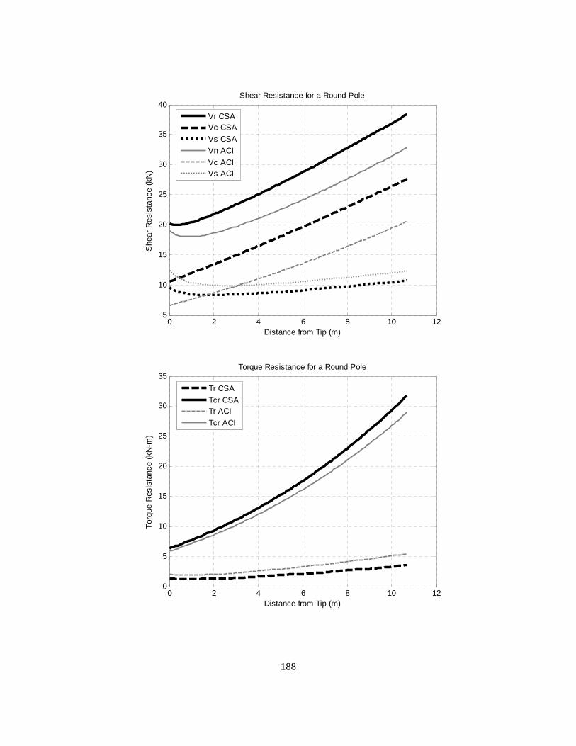
188

0 2 4 6 8 10 125

10

15

20

25

30

35

40


She

ar R

esis

tanc

e (k

N)



0 2 4 6 8 10 120

5

10

15

20

25

30

35


Torq

ue R

esis

tanc

e (k

N-m

)



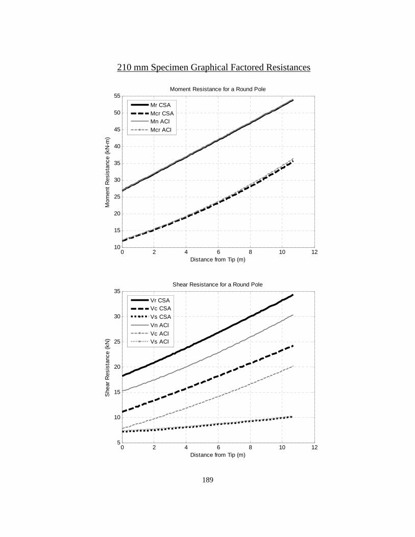
189

210 mm Specimen Graphical Factored Resistances

0 2 4 6 8 10 1210

15

20

25

30

35

40

45

50

55


Mom

ent R

esis

tanc

e (k

N-m

)



0 2 4 6 8 10 125

10

15

20

25

30

35


She

ar R

esis

tanc

e (k

N)



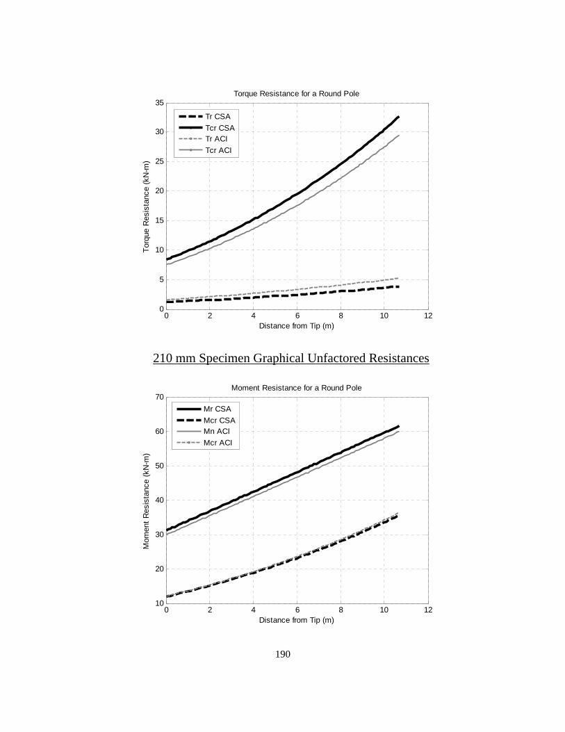
190

0 2 4 6 8 10 120

5

10

15

20

25

30

35


Torq

ue R

esis

tanc

e (k

N-m

)



210 mm Specimen Graphical Unfactored Resistances

0 2 4 6 8 10 1210

20

30

40

50

60

70


Mom

ent R

esis

tanc

e (k

N-m

)



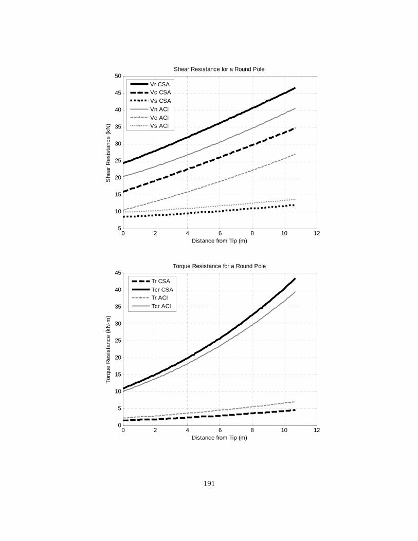
191

0 2 4 6 8 10 125

10

15

20

25

30

35

40

45

50


She

ar R

esis

tanc

e (k

N)



0 2 4 6 8 10 120

5

10

15

20

25

30

35

40

45


Torq

ue R

esis

tanc

e (k

N-m

)



192

Appendix B Specimen Material Reports

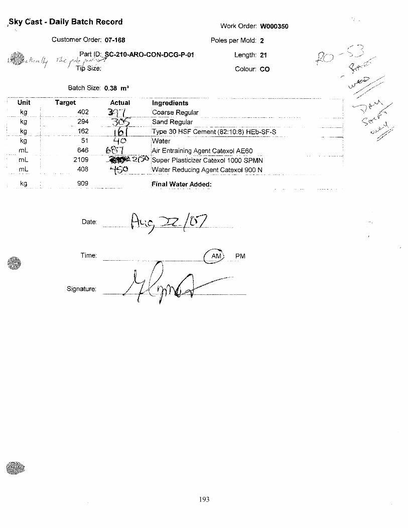
193

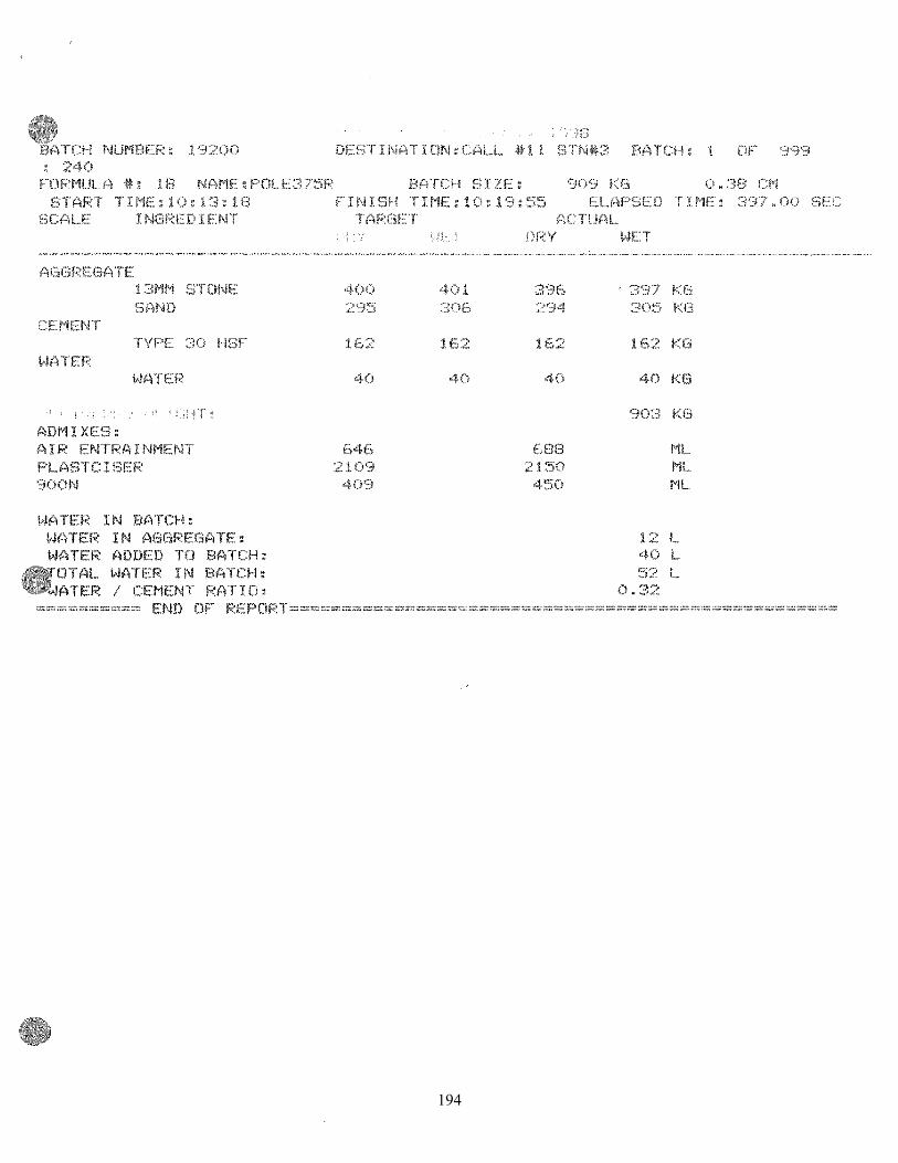
194

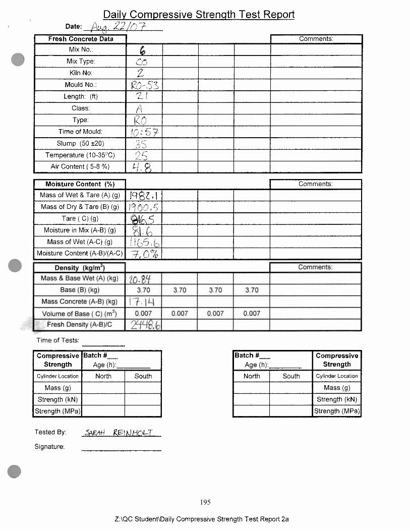
195

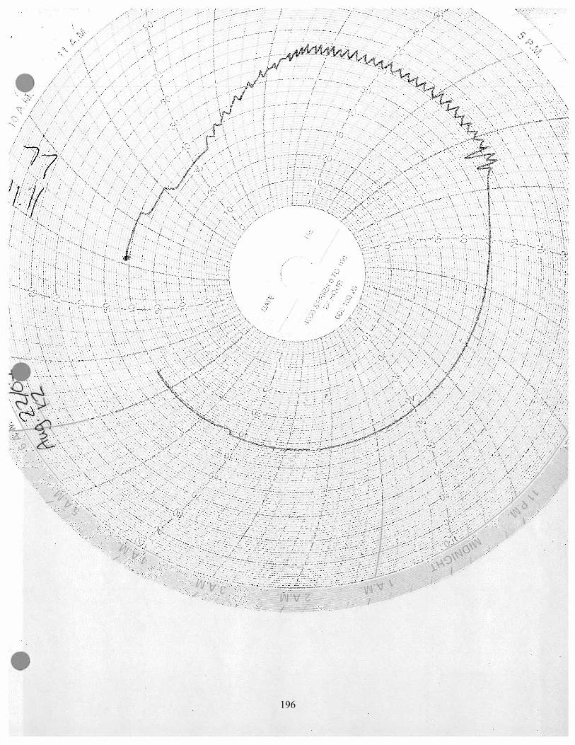
196

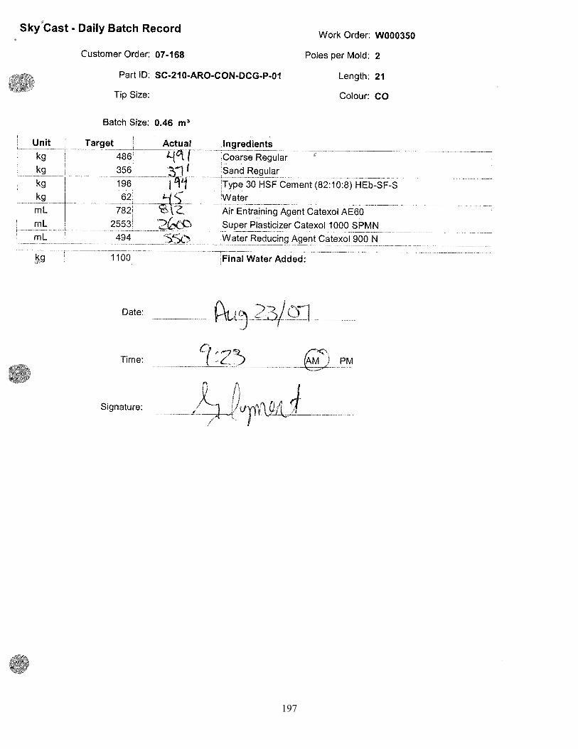
197

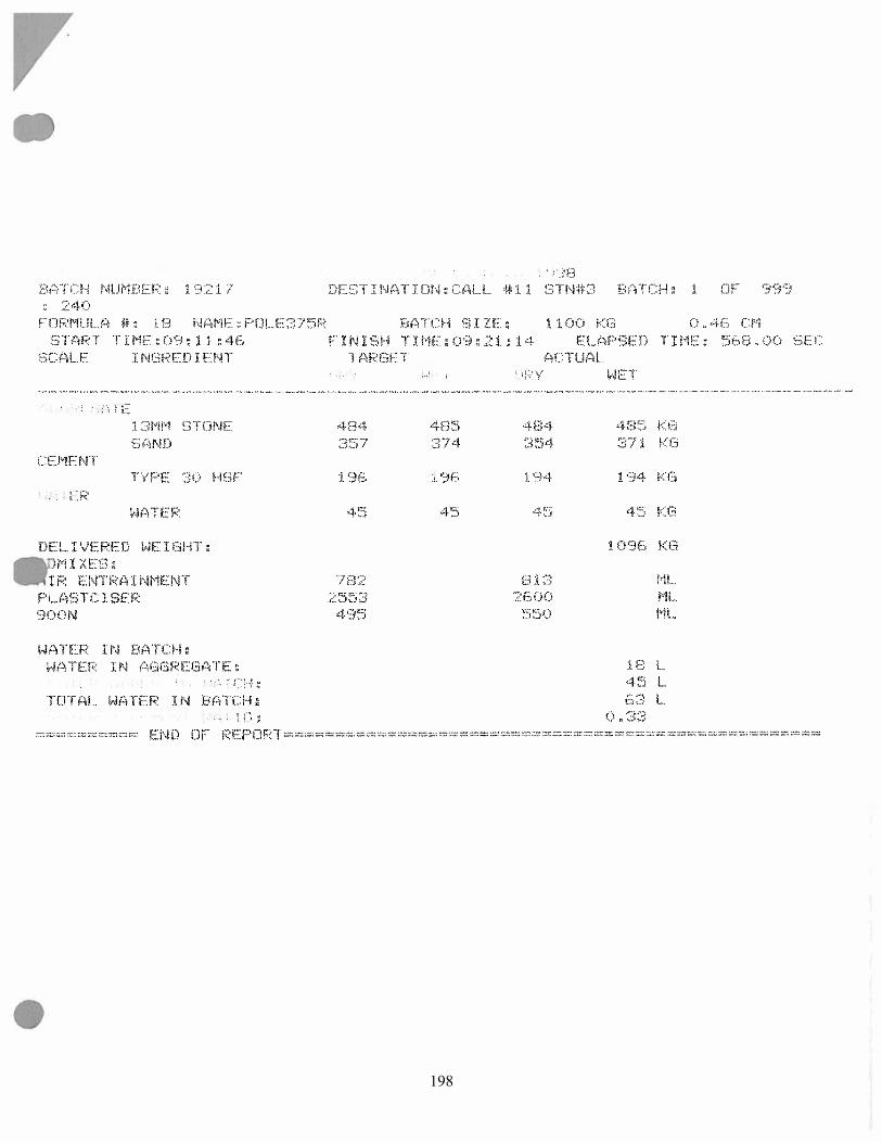
198

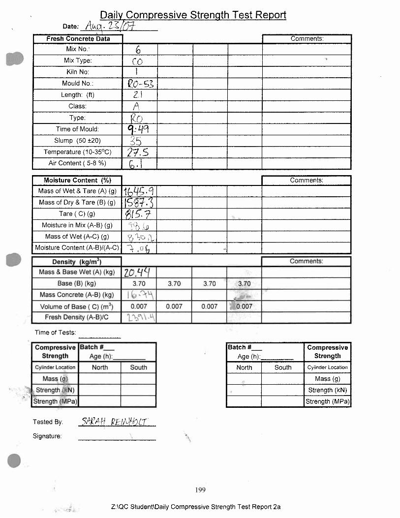
199

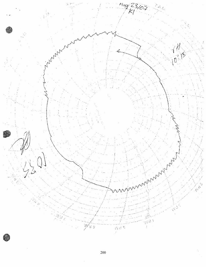
200

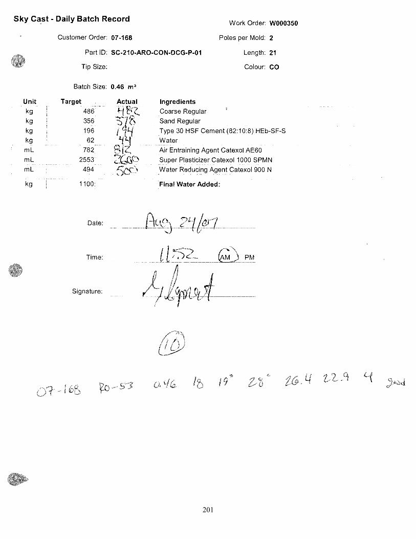
201

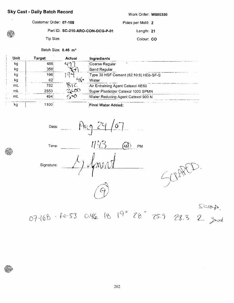
202

203

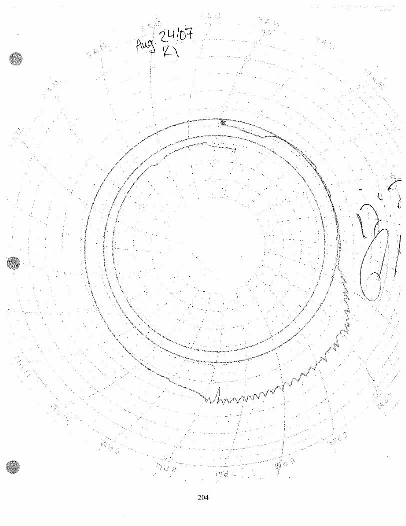
204

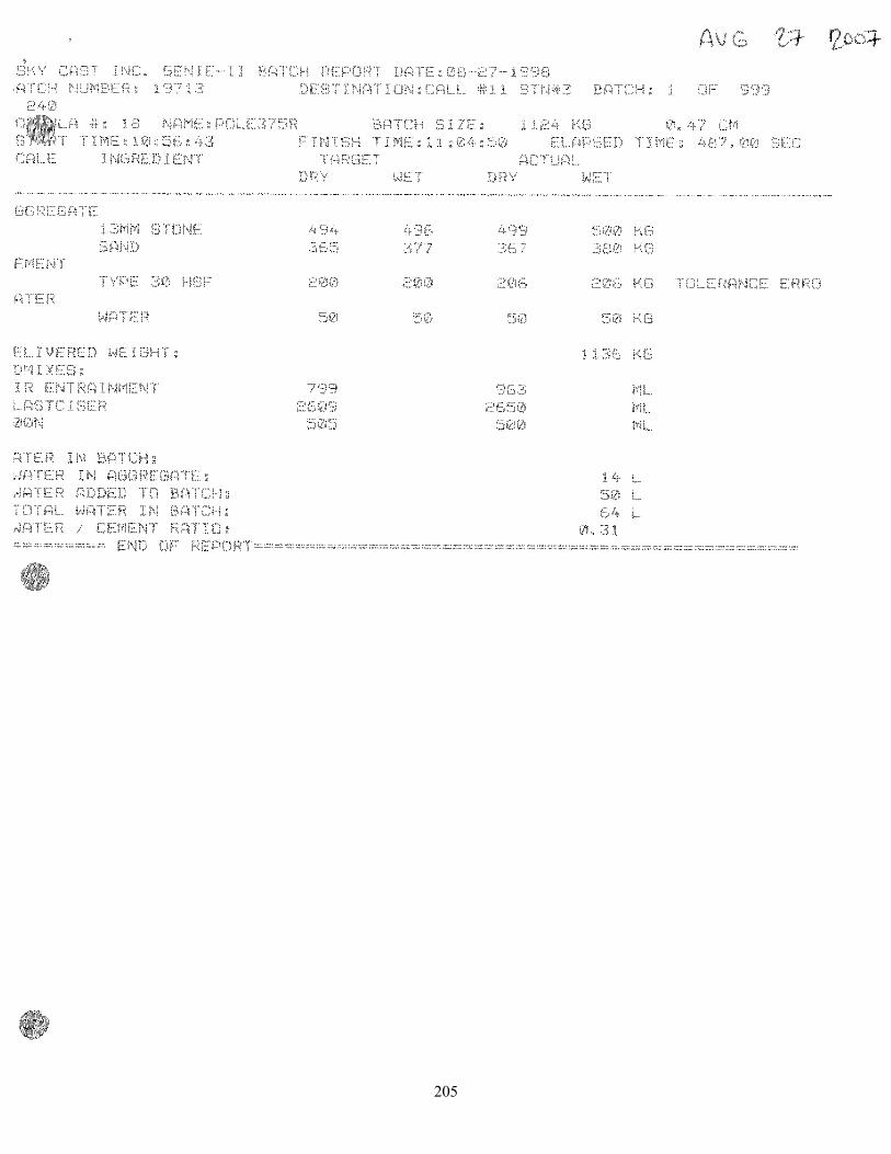
205

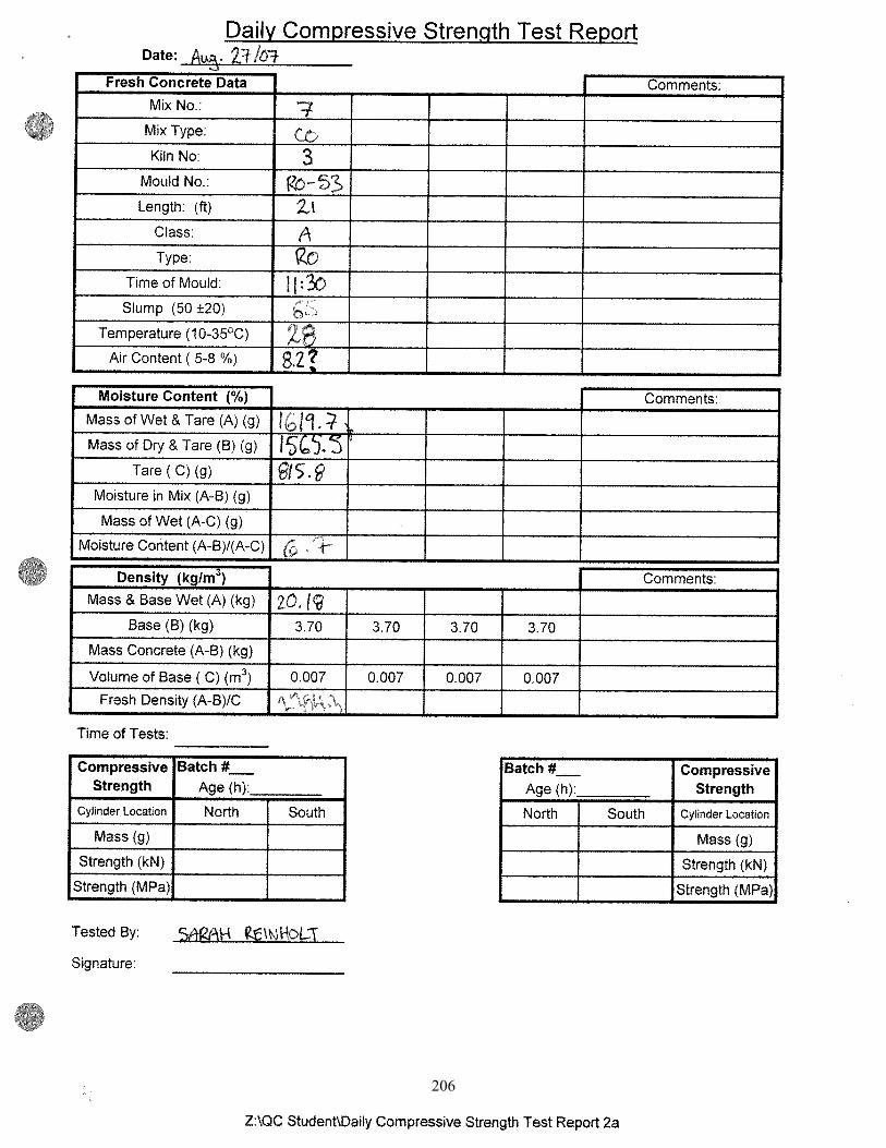
206

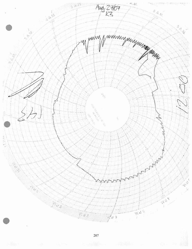
207

208

209

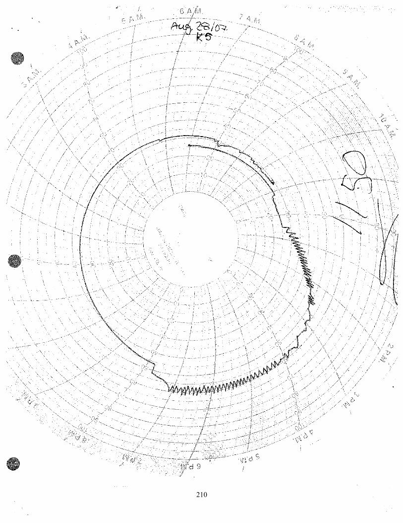
210

211

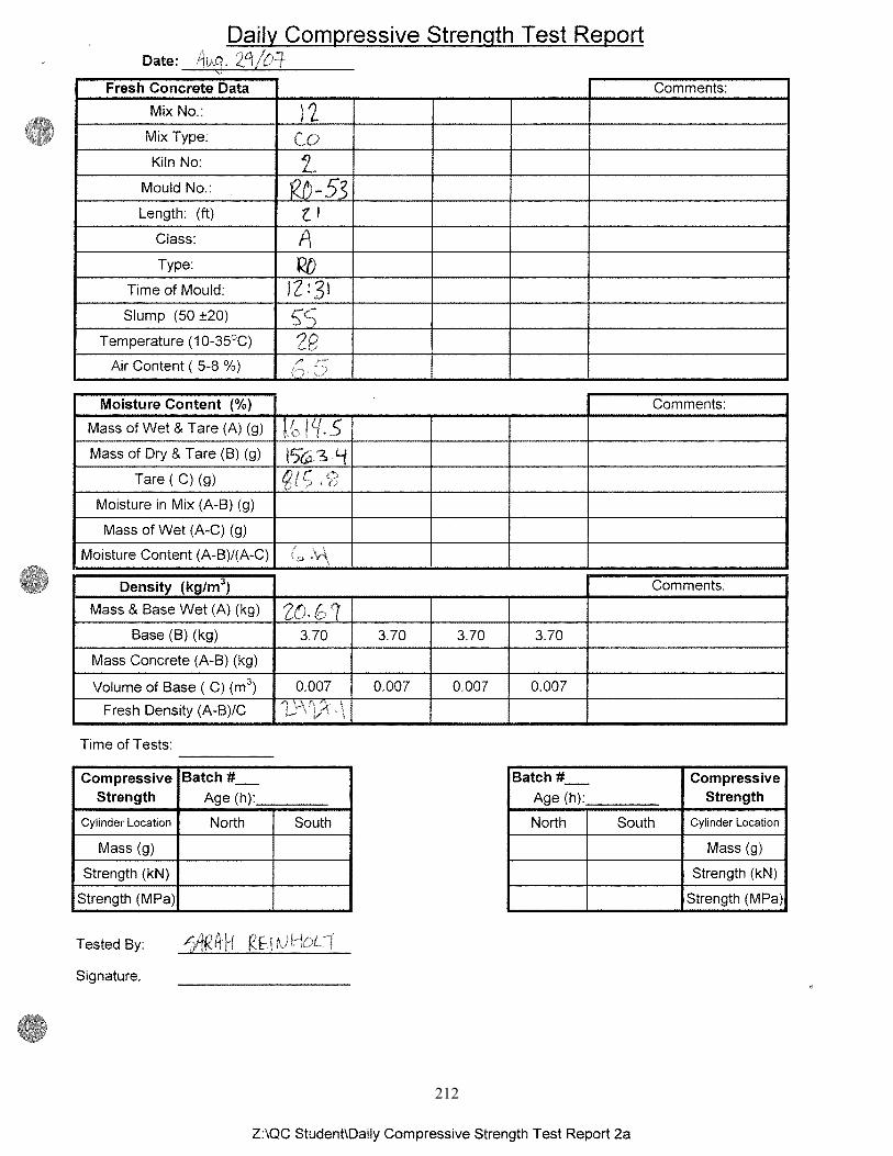
212

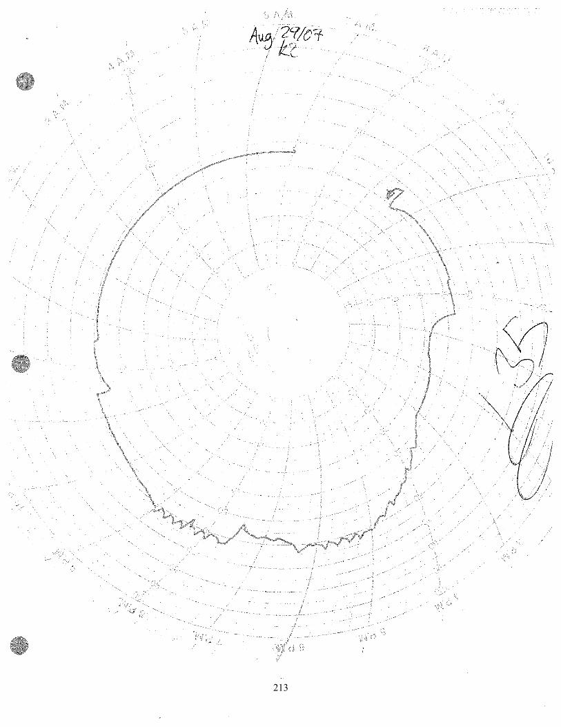
213

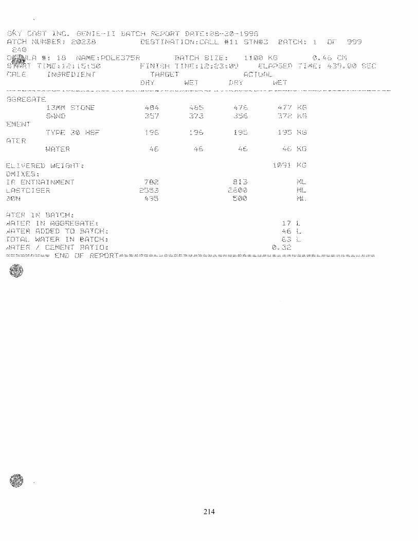
214

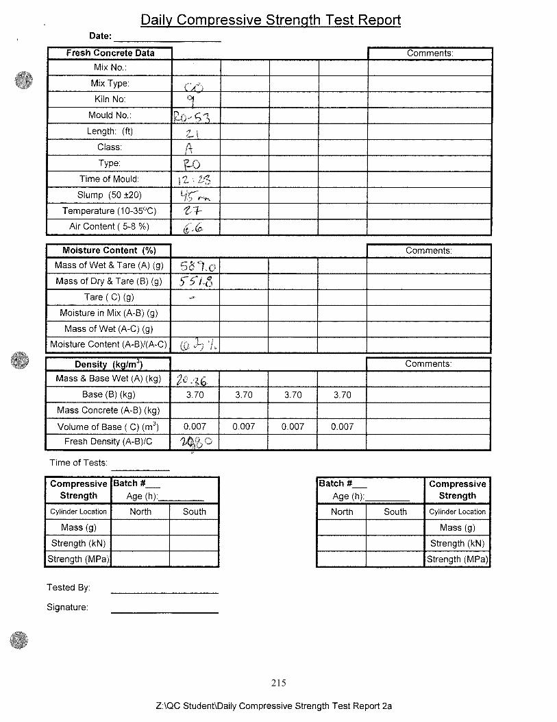
215

216

217

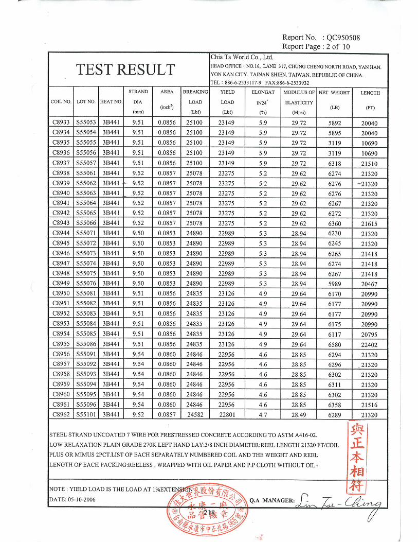
218

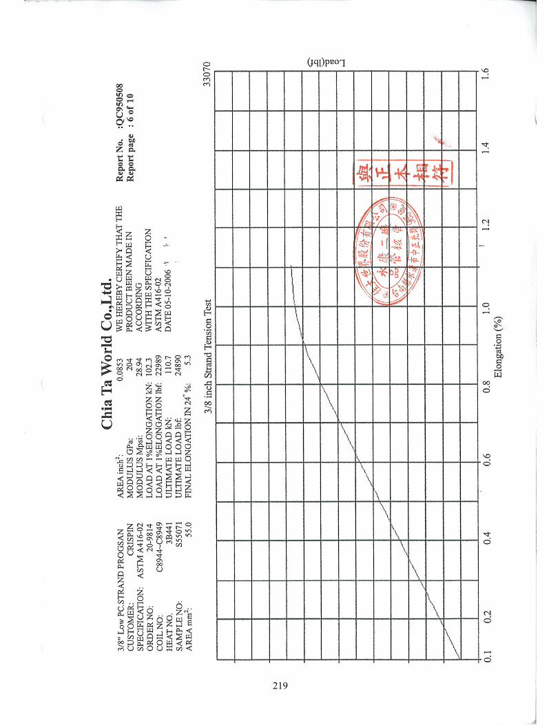
219

220

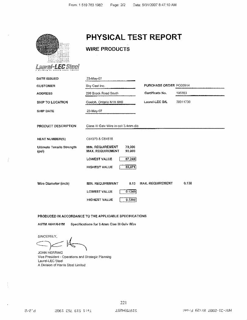
221

222

Appendix C Testing Raw Data Sheets

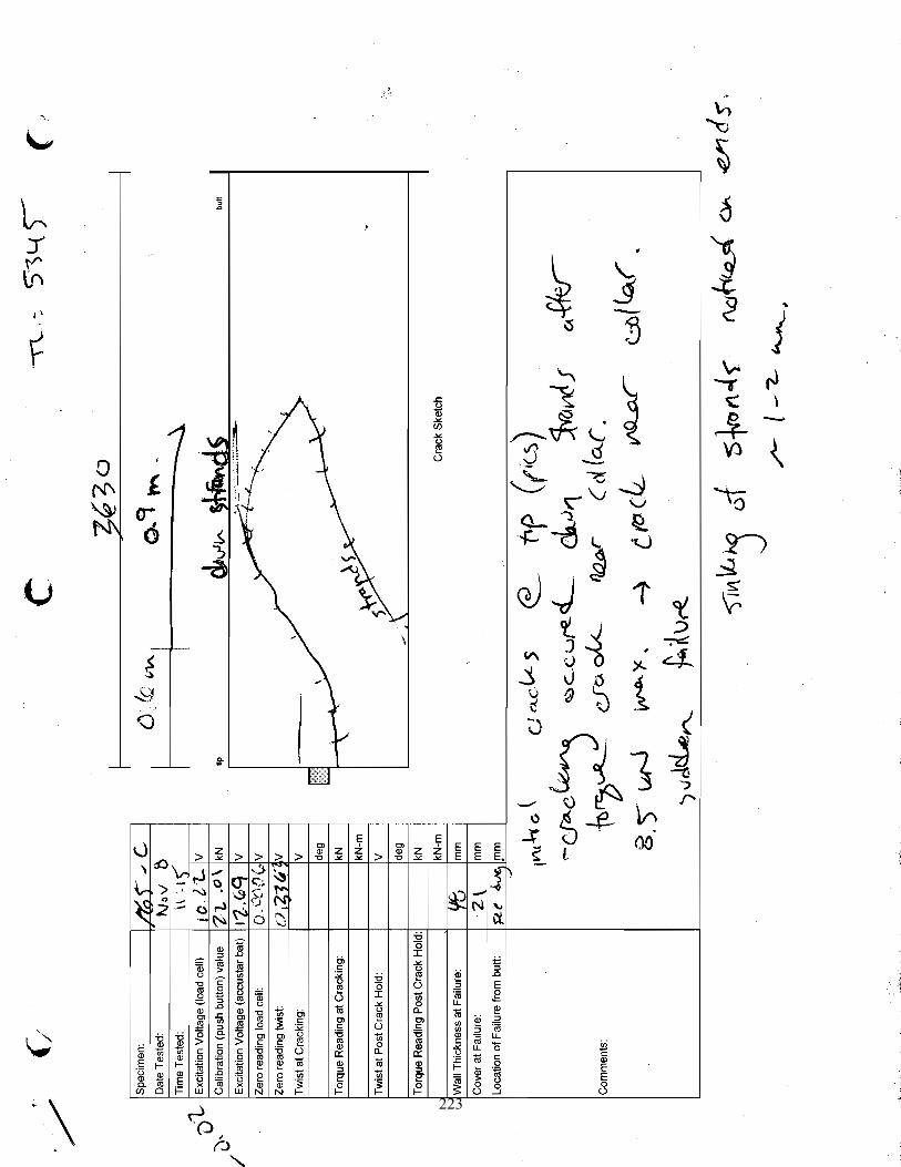
223

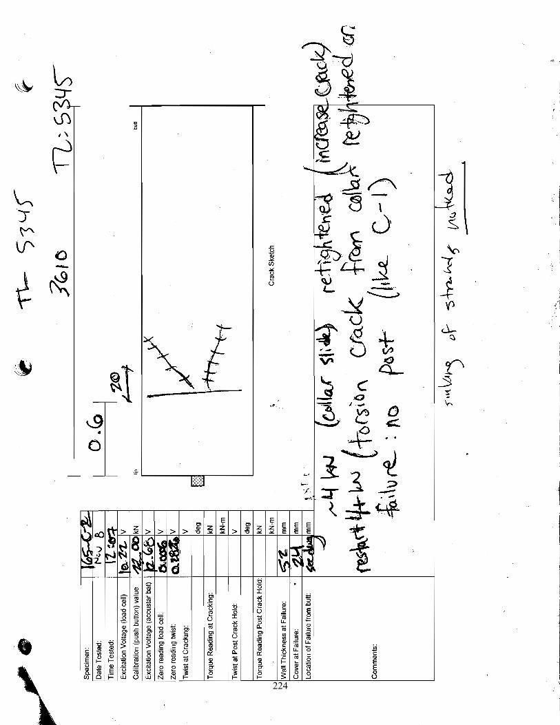
224

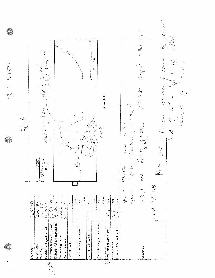
225

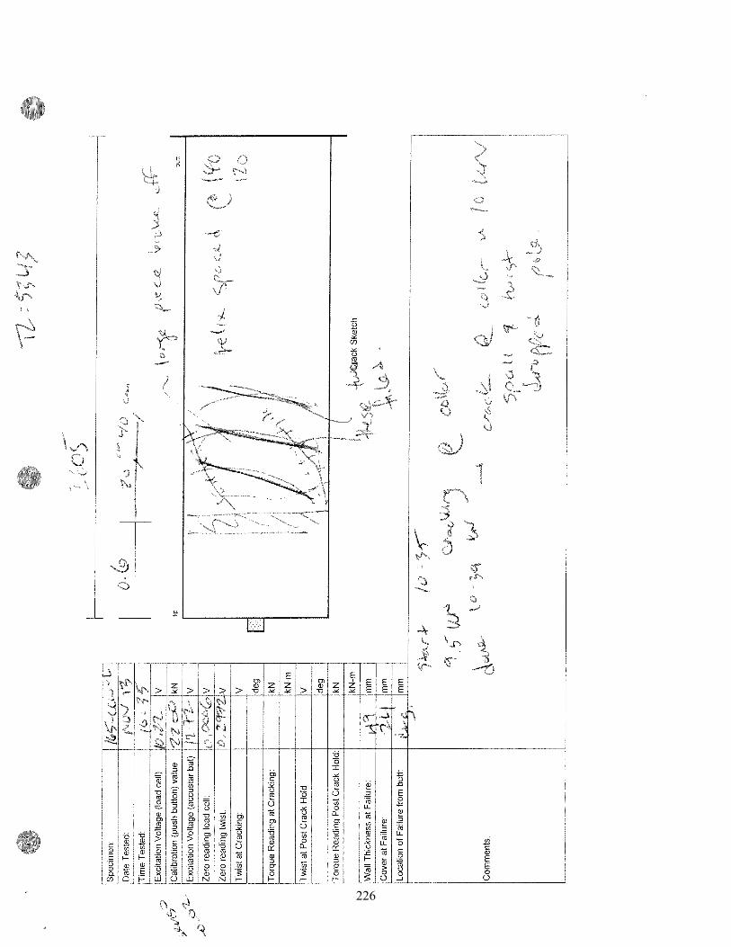
226

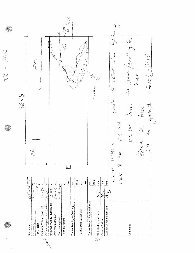
227

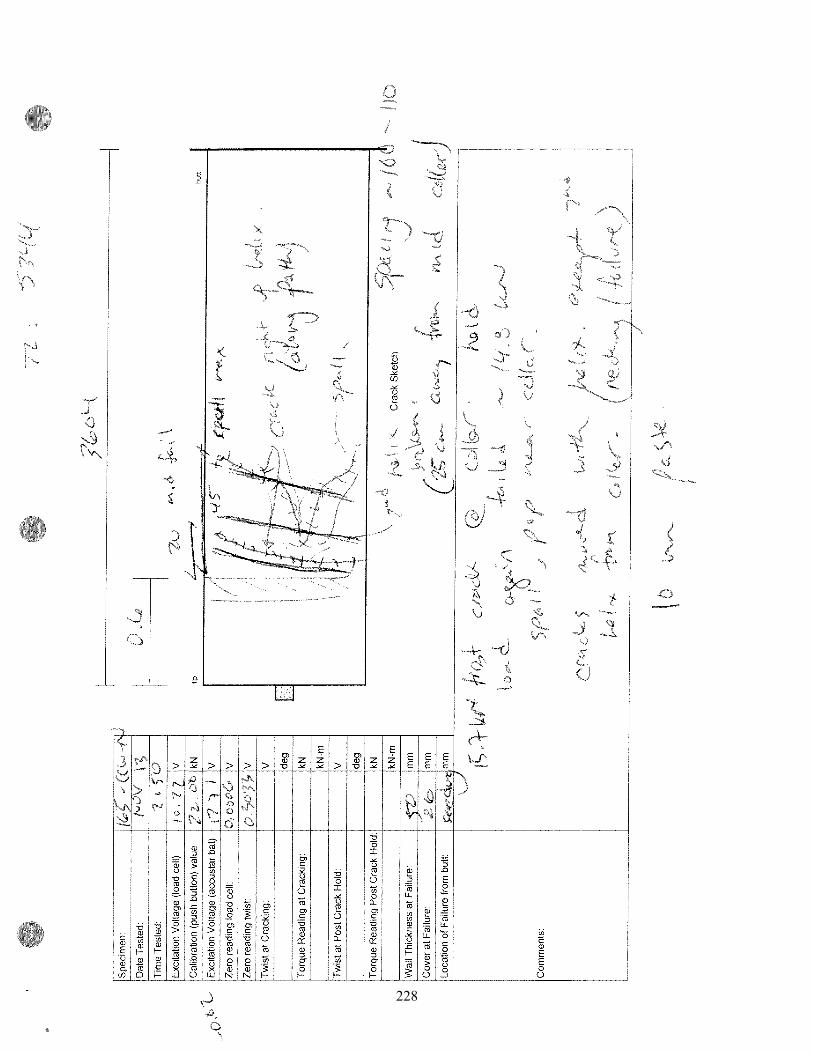
228

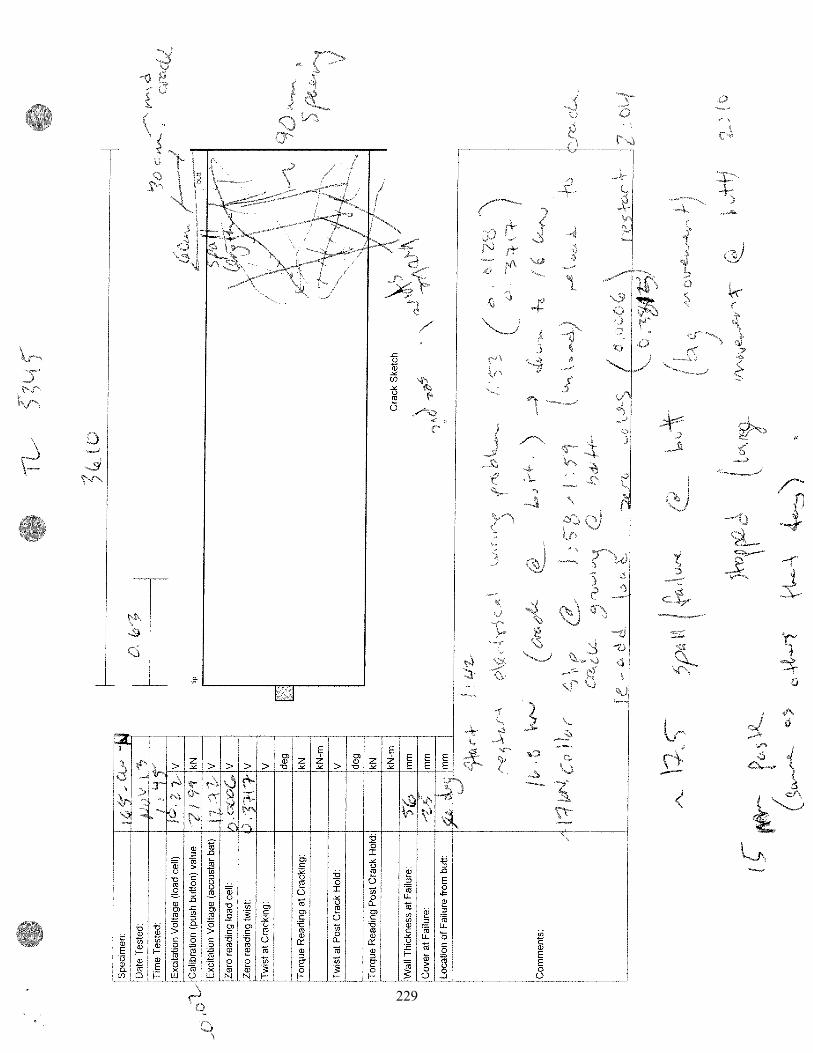
229

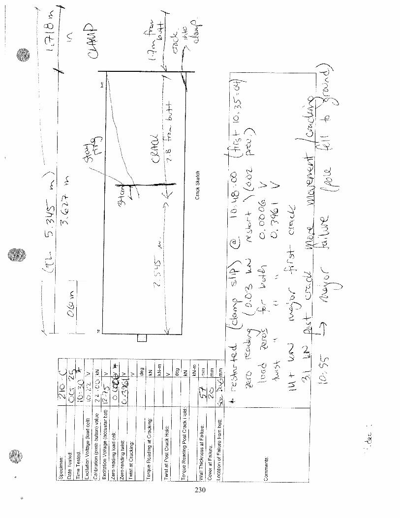
230

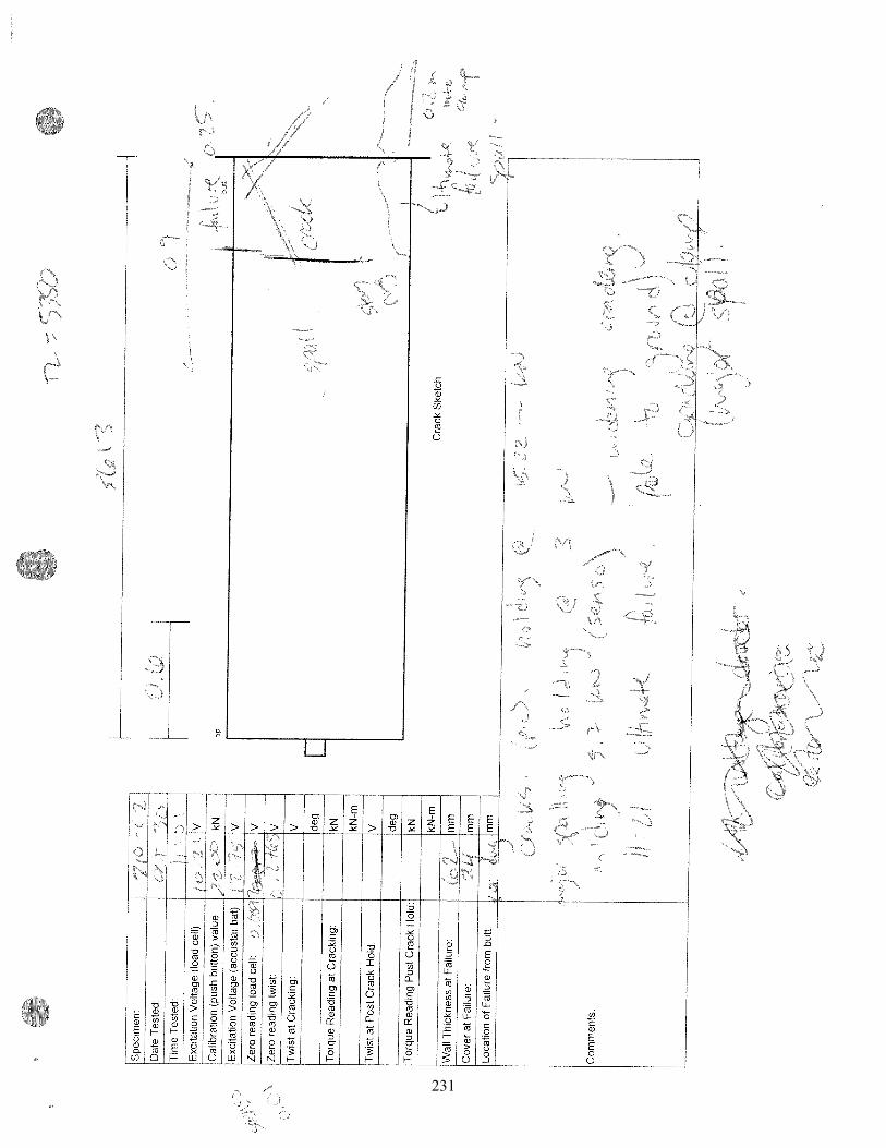
231

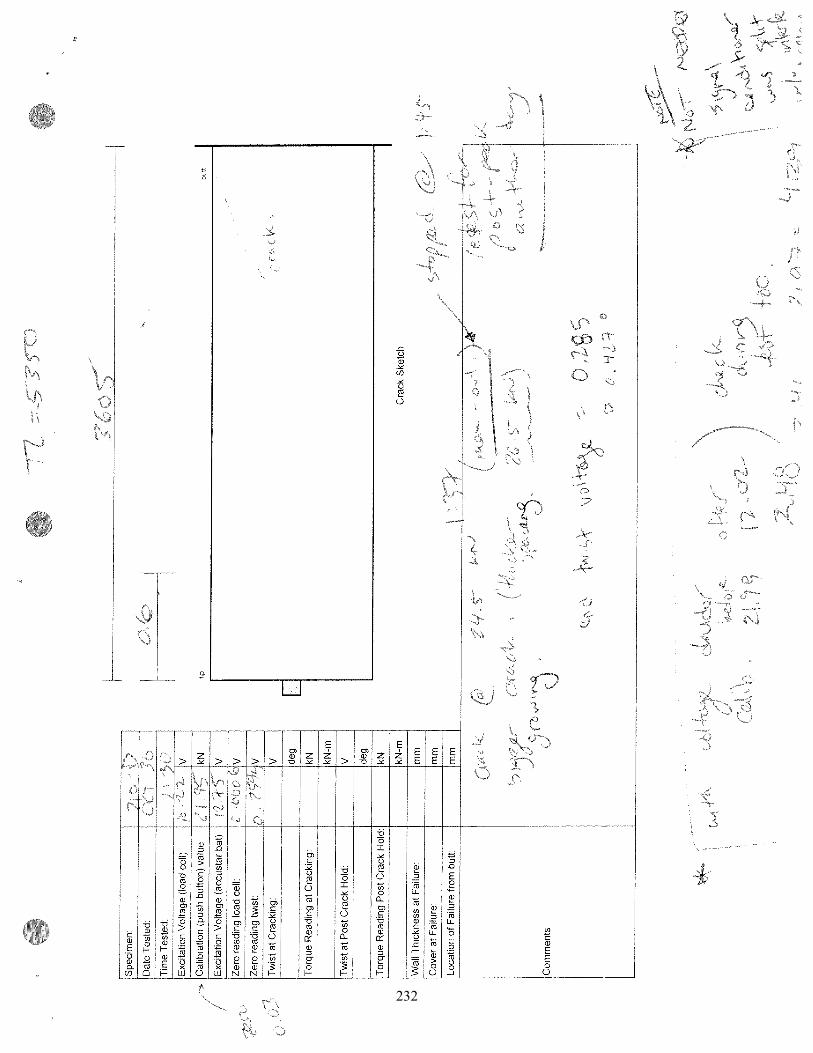
232

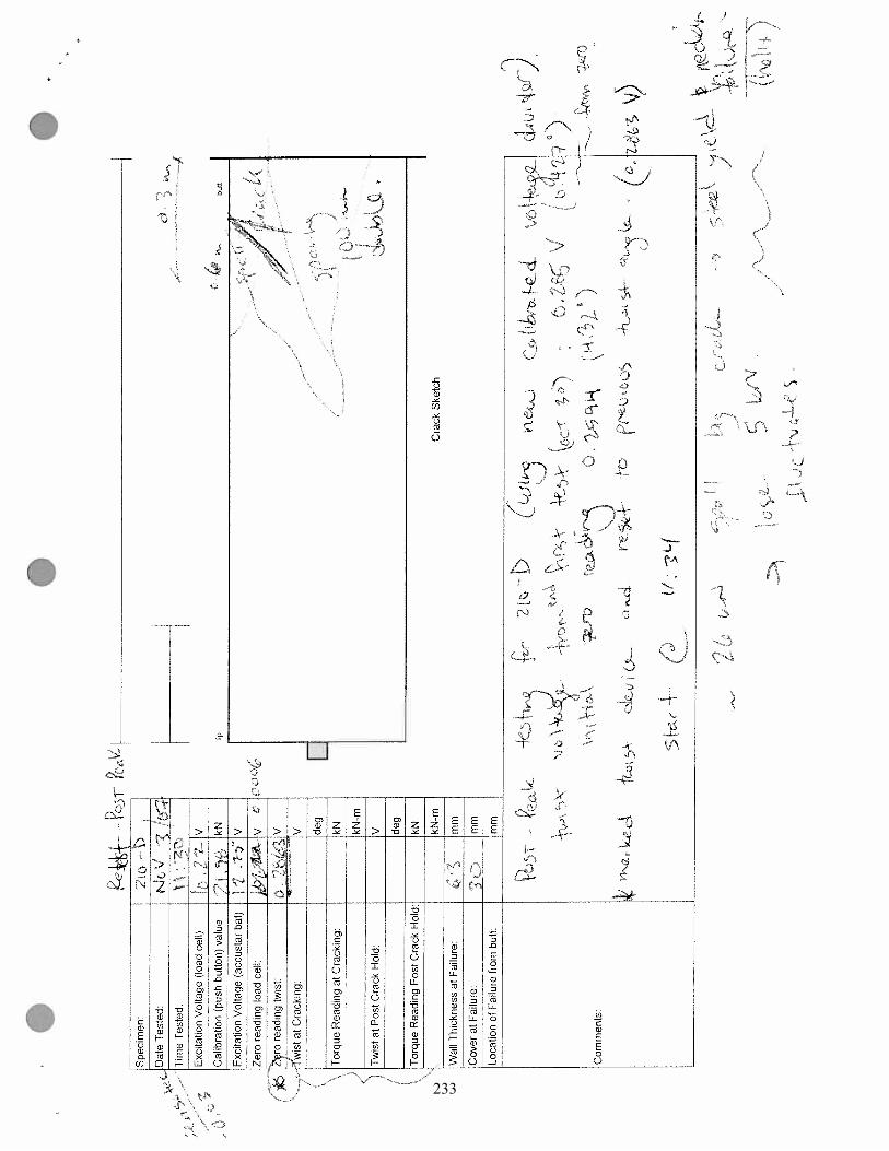
233

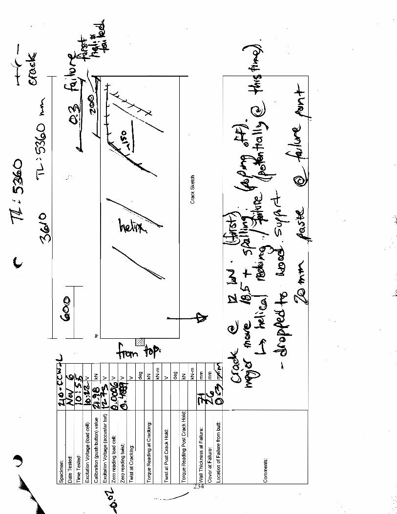
234

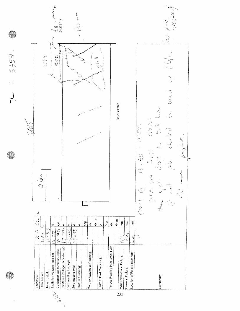
235

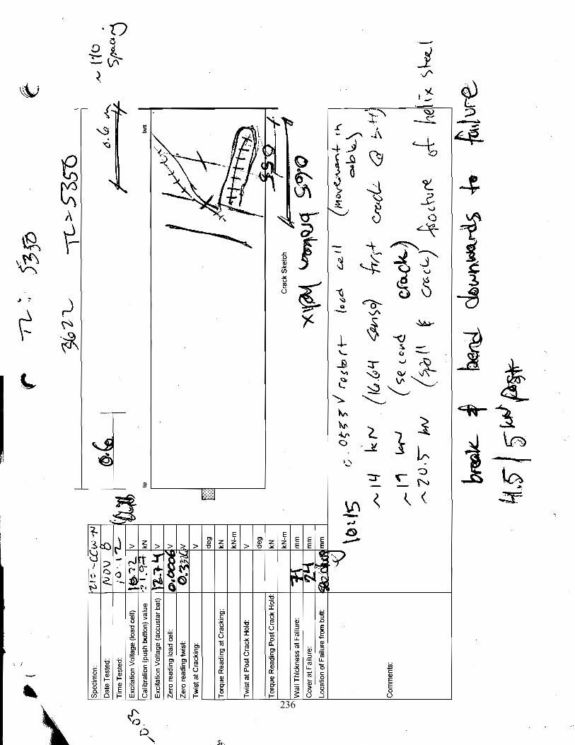
236

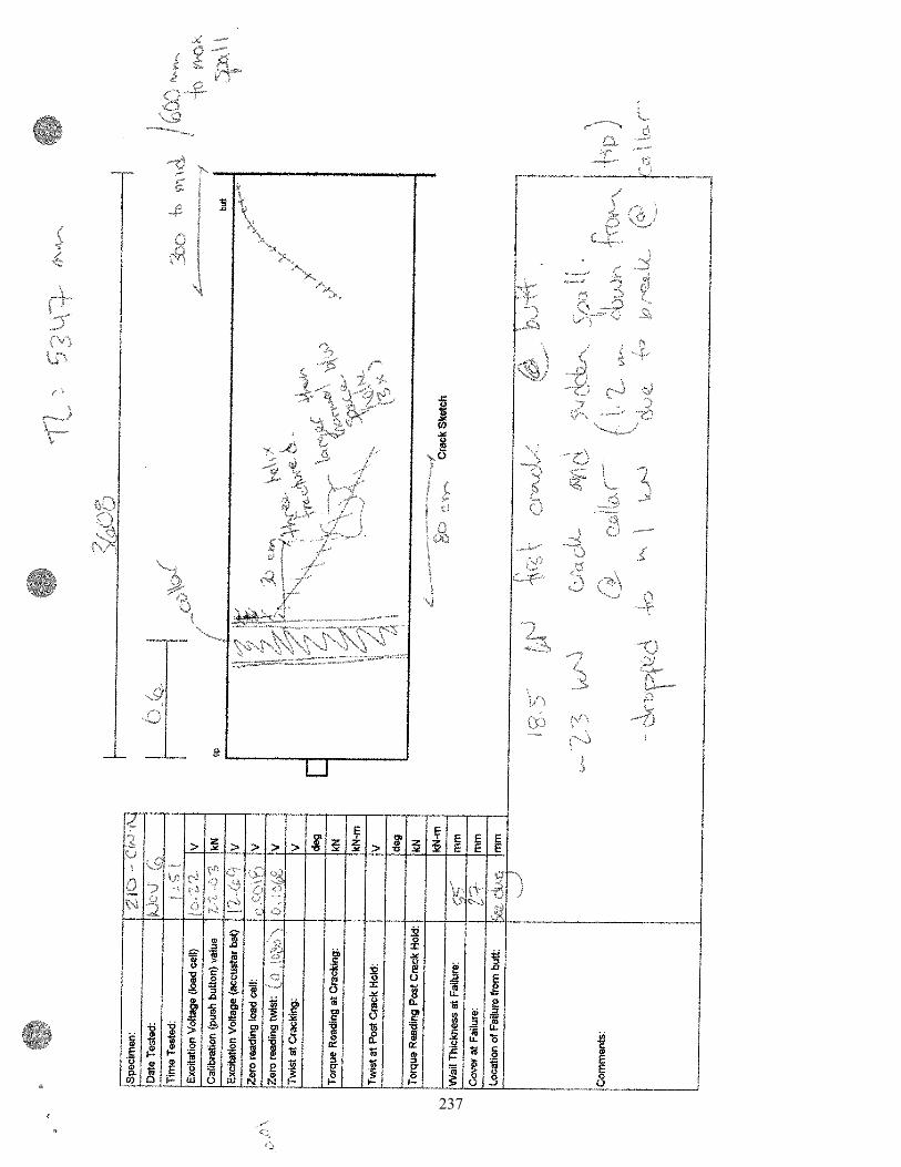
237

238

Appendix D Strut and Tie Model and Code Maximum Spacing Calculations

Stru

t and

Tie

Cal

cula

tion

for T

rans

fer L

engt

h of

Con

cret

e P

ole

- Poi

nt S

trand

Loa

d

fpu

1860

Mpa

phi p

1fp

i13

39.2

Mpa

(20

% lo

sses

, stre

ssed

to 9

0%)

Ass

ume

fci =

25M

pa@

tran

sfer

Ap

(one

stra

nd)

55.2

3m

m^2

9.52

mm

tip d

iam

eter

210

mm

wal

l thi

ckne

ss55

mm

p - e

ff99

perim

eter

(dia

met

er)

Tape

r15

mm

/mw

- ef

f42

wal

l thi

ckne

sstra

nsfe

r len

gth

=47

6m

mX

-sec

tion

(Ac)

2678

2.07

737

mm

^2ph

i s1

fy50

0M

Pa

Pi =

73.9

6kN

db3.

5m

mP

i/L0.

16kN

/mm

As

9.62

mm

^2

Ass

umed

s

Dia

met

erat

incr

emen

tlo

adw

all

thic

knes

s

1/4

cent

erlin

epe

rimet

eras

sum

ed s

- s

p-ef

fw

-eff

angl

e of

st

rut (

deg)

s

Pin

crem

ent

al (k

N)

C in

stru

t (k

N)

Cr (

kN)

T (k

N)

Tr (k

N)

angl

e of

re

info

rcem

ent

Tr -

redu

ced

(kN

)

T / T

r re

duce

d #

need

edIn

crem

ent

47.1

221

0.71

55.0

012

2.29

-5.9

599

4225

53.0

88.

254.

553.

681.

924.

8182

.80

4.77

0.40

9942

4524

.75

3.85

2.72

1.72

1.92

4.81

86.6

34.

800.

4099

4265

11.5

41.

792.

120.

801.

924.

8188

.43

4.81

0.40

#DIV

/0!

1.65

MP

a6.

0144

62kN

take

pre

stre

ss2.

6980

1818

MP

aw

t16

.969

3254

mm

Che

ck s

truts

Com

pute

wid

th o

f stru

ts A

BN

ode

A is

CC

Cal

pha

E1

phi c

* fc

u m

ax =

0.8

5*f c

fcu

assu

me

wal

l thi

ckne

ssw

sE

nd A

650.

0028

719

.421

.25

19.4

428.

645

0.00

613

.721

.25

13.7

427.

325

0.02

0396

5.9

21.2

55.

942

13.3

Nod

e B

is C

CT

max

= 0

.75*

fcu

End

B65

0.00

287

19.4

18.7

518

.75

428.

945

0.00

613

.718

.75

13.7

3626

3742

7.3

250.

0203

965.

918

.75

5.85

8562

4213

.3

SU

MM

AR

Y

Stru

tsTi

esA

ngle

ws

End

Aw

s E

nd B

# tie

ss

OR

Con

cret

e Ti

e25

8.6

8.9

mm

9.0

5317

.0m

m45

7.3

7.3

mm

19.2

2517

.0m

m65

13.3

13.3

mm

4112

17.0

mm

239

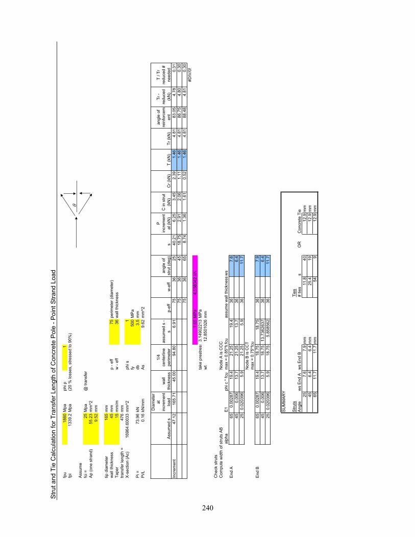
Stru

t and

Tie

Cal

cula

tion

for T

rans

fer L

engt

h of

Con

cret

e P

ole

- Poi

nt S

trand

Loa

d

fpu

1860

Mpa

phi p

1fp

i13

39.2

Mpa

(20

% lo

sses

, stre

ssed

to 9

0%)

Ass

ume

fci =

25M

pa@

tran

sfer

Ap

(one

stra

nd)

55.2

3m

m^2

9.52

mm

tip d

iam

eter

165

mm

wal

l thi

ckne

ss45

mm

p - e

ff75

perim

eter

(dia

met

er)

Tape

r15

mm

/mw

- ef

f36

wal

l thi

ckne

sstra

nsfe

r len

gth

=47

6m

mX

-sec

tion

(Ac)

1696

4.60

033

mm

^2ph

i s1

fy50

0M

Pa

Pi =

73.9

6kN

db3.

5m

mP

i/L0.

16kN

/mm

As

9.62

mm

^2

Ass

umed

s

Dia

met

erat

incr

emen

tlo

adw

all

thic

knes

s

1/4

cent

erlin

epe

rimet

eras

sum

ed s

- s

p-ef

fw

-eff

angl

e of

st

rut (

deg)

s

Pin

crem

ent

al (k

N)

C in

stru

t (k

N)

Cr (

kN)

T (k

N)

Tr (k

N)

angl

e of

re

info

rcem

ent

Tr -

redu

ced

(kN

)

T / T

r re

duce

d #

need

edIn

crem

ent

47.1

216

5.71

45.0

094

.80

6.91

7536

2540

.21

6.25

3.45

2.39

1.46

4.81

83.0

54.

780.

3175

3645

18.7

52.

912.

061.

111.

464.

8186

.75

4.80

0.30

7536

658.

741.

361.

610.

521.

464.

8188

.48

4.81

0.30

#DIV

/0!

1.65

MP

a4.

5583

42kN

take

pre

stre

ss3.

1490

2213

MP

aw

t12

.850

1026

mm

Che

ck s

truts

Com

pute

wid

th o

f stru

ts A

BN

ode

A is

CC

Cal

pha

E1

phi c

* fc

u m

ax =

0.8

5*f c

fcu

assu

me

wal

l thi

ckne

ssw

sE

nd A

650.

0028

719

.421

.25

19.4

367.

645

0.00

613

.721

.25

13.7

366.

425

0.02

0396

5.9

21.2

55.

936

11.7

Nod

e B

is C

CT

max

= 0

.75*

fcu

End

B65

0.00

287

19.4

18.7

518

.75

367.

945

0.00

613

.718

.75

13.7

3626

3736

6.4

250.

0203

965.

918

.75

5.85

8562

3611

.7

SU

MM

AR

Y

Stru

tsTi

esA

ngle

ws

End

Aw

s E

nd B

# tie

ss

OR

Con

cret

e Ti

e25

7.6

7.9

mm

11.8

4012

.9m

m45

6.4

6.4

mm

25.4

1912

.9m

m65

11.7

11.7

mm

549

12.9

mm

240

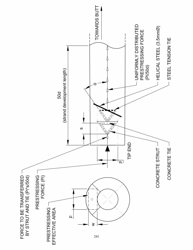
241

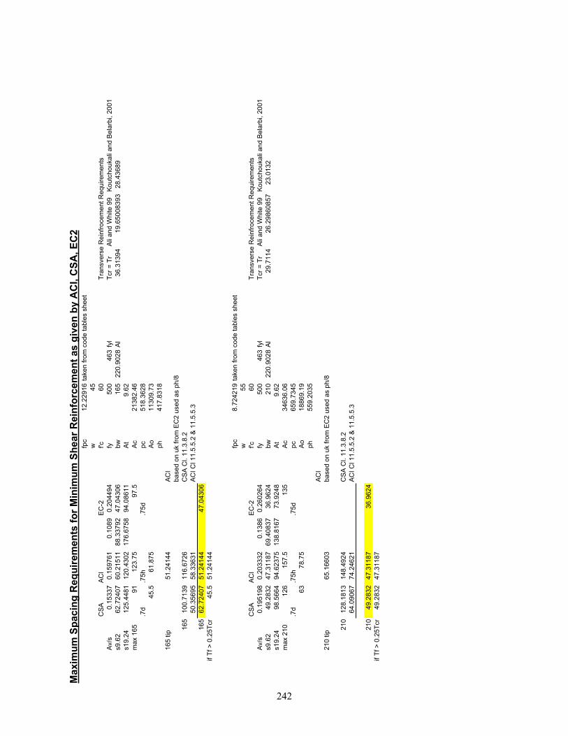
Max

imum

Spa

cing

Req

uire

men

ts fo

r Min

imum

She

ar R

einf

orce

men

t as

give

n by

AC

I, C

SA, E

C2

fpc

12.2

2916

take

n fro

m c

ode

tabl

es s

heet

w45

CS

AA

CI

EC

-2f'c

60Tr

ansv

erse

Rei

nfro

cem

ent R

equi

rem

ents

Av/

s0.

1533

70.

1597

610.

1089

0.20

4494

fy50

046

3fy

lTc

r = T

rA

li an

d W

hite

99

Kou

tcho

ukal

i and

Bel

arbi

, 200

1s9

.62

62.7

2407

60.2

1511

88.3

3792

47.0

4306

bw16

522

0.90

28A

l36

.313

9419

.650

0839

328

.436

89s1

9.24

125.

4481

120.

4302

176.

6758

94.0

8611

At

9.62

max

165

9112

3.75

97.5

Ac

2138

2.46

.7d

.75h

.75d

pc51

8.36

2845

.561

.875

Ao

1130

9.73

ph41

7.83

1816

5 tip

51.2

4144

AC

Iba

sed

on u

k fro

m E

C2

used

as

ph/8

165

100.

7139

116.

6726

CS

A C

l. 11

.3.8

.250

.356

9558

.336

31A

CI C

l 11.

5.5.

2 &

11.

5.5.

316

562

.724

0751

.241

4447

.043

06if

Tf >

0.2

5Tcr

45.5

51.2

4144

fpc

8.72

4219

take

n fro

m c

ode

tabl

es s

heet

w55

CS

AA

CI

EC

-2f'c

60Tr

ansv

erse

Rei

nfro

cem

ent R

equi

rem

ents

Av/

s0.

1951

980.

2033

320.

1386

0.26

0264

fy50

046

3fy

lTc

r = T

rA

li an

d W

hite

99

Kou

tcho

ukal

i and

Bel

arbi

, 200

1s9

.62

49.2

832

47.3

1187

69.4

0837

36.9

624

bw21

022

0.90

28A

l29

.711

426

.298

6085

723

.013

2s1

9.24

98.5

664

94.6

2375

138.

8167

73.9

248

At

9.62

max

210

126

157.

513

5A

c34

636.

06.7

d.7

5h.7

5dpc

659.

7345

6378

.75

Ao

1886

9.19

ph55

9.20

35A

CI

210

tip65

.166

03ba

sed

on u

k fro

m E

C2

used

as

ph/8

210

128.

1813

148.

4924

CS

A C

l. 11

.3.8

.264

.090

6774

.246

21A

CI C

l 11.

5.5.

2 &

11.

5.5.

3

210

49.2

832

47.3

1187

36.9

624

if Tf

> 0

.25T

cr49

.283

247

.311

87

242

243

Appendix E Typical Fixture Product Sheets and Wind Load Calculations

244

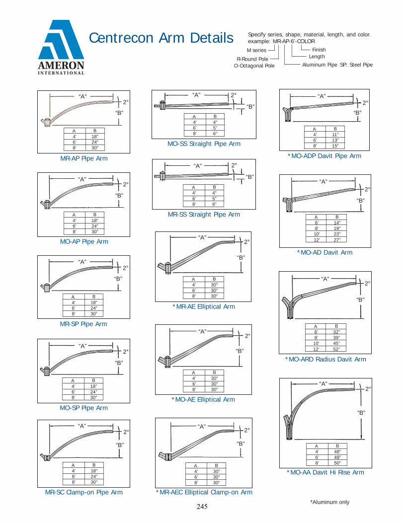
*MO-AD Davit Arm

*MO-ADP Davit Pipe Arm

MR-SS Straight Pipe Arm

MO-SS Straight Pipe Arm

*MO-AA Davit Hi Rise Arm

*MR-AE Elliptical Arm

*MO-AE Elliptical Arm

*MR-AEC Elliptical Clamp-on Arm

*MO-ARD Radius Davit Arm

MR-SP Pipe Arm

MO-SP Pipe Arm

MR-SC Clamp-on Pipe Arm

“A”

“B”

2°

“A”

“B”

2°

“A”2°

“B”

MO-AP Pipe Arm

“A”

“B”

2°

MR-AP Pipe Arm

“A”

“B”

2°

“A”

“B”

2°

“A”

“B”

2°

“A”

“B”

2°

“A”

“B”

2°

“A”

“B”

2°

“A”

“B”

2°

“A”

“B”

2°

“A”

“B”

2°

“A”

“B”

2°

Specify series, shape, material, length, and color.example: MR-AP-6’-COLOR

M series

R-Round PoleO-Octagonal Pole

FinishLength

Aluminum Pipe SP: Steel Pipe

Centrecon Arm Details

*Aluminum only

A4’6’8’

B18”24”30”

A4’6’8’

B18”24”30”

A4’6’8’

B18”24”30”

A4’6’8’

B18”24”30”

A4’6’8’

B18”24”30”

A4’6’8’

B30”30”30”

A4’6’8’

B30”30”30”

A4’6’8’

B30”30”30”

A4’6’8’

B4”5”6”

A4’6’8’

B4”5”6”

A4’6’8’

B11”13”15”

A4’6’8’

B48”49”50”

A6’8’

10’

B14”19”23”

12’ 27”

A6’8’

10’

B32”39”45”

12’ 52”

245

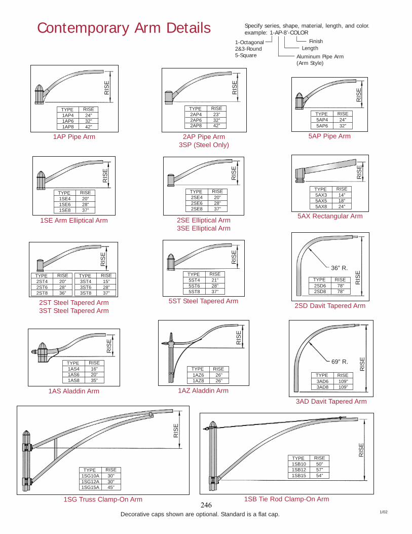
Contemporary Arm Details

2ST Steel Tapered Arm3ST Steel Tapered Arm

5ST Steel Tapered Arm

2AP Pipe Arm3SP (Steel Only)

1AP Pipe Arm 5AP Pipe Arm

1SE Arm Elliptical Arm 2SE Elliptical Arm3SE Elliptical Arm

1AS Aladdin Arm 1AZ Aladdin Arm

2SD Davit Tapered Arm

3AD Davit Tapered Arm

5AX Rectangular Arm

1SB Tie Rod Clamp-On Arm1SG Truss Clamp-On Arm

RIS

E

RIS

E

RIS

E

RIS

E

RIS

E

RIS

E

RIS

E

RIS

E

RIS

E

RIS

E RIS

E

RIS

E

36” R.

RIS

E69” R.R

ISE

Specify series, shape, material, length, and color.example: 1-AP-8’-COLOR

1-Octagonal2&3-Round5-Square

FinishLength

Aluminum Pipe Arm(Arm Style)

TYPE1SE41SE61SE8

RISE20”28”37”

TYPE2SE42SE62SE8

RISE20”28”37”

TYPE5AP45AP6

RISE24”32”

TYPE2AP42AP62AP8

RISE23”32”42”

TYPE1AP41AP61AP8

RISE24”32”42”

TYPE1AS41AS61AS8

RISE16”20”35”

TYPE1AZ61AZ8

RISE26”26”

TYPE2SD62SD8

RISE78”78”

TYPE3AD63AD8

RISE109”109”

TYPE2ST42ST62ST8

RISE20”28”36”

TYPE3ST43ST63ST8

RISE15”28”37”

TYPE5ST45ST65ST8

RISE21”28”37”

TYPE5AX35AX55AX8

RISE14”18”24”

TYPE1SB101SB121SB15

RISE50”57”54”

TYPE1SG10A1SG12A1SG15A

RISE30”30”45”

Decorative caps shown are optional. Standard is a flat cap. 1/02246

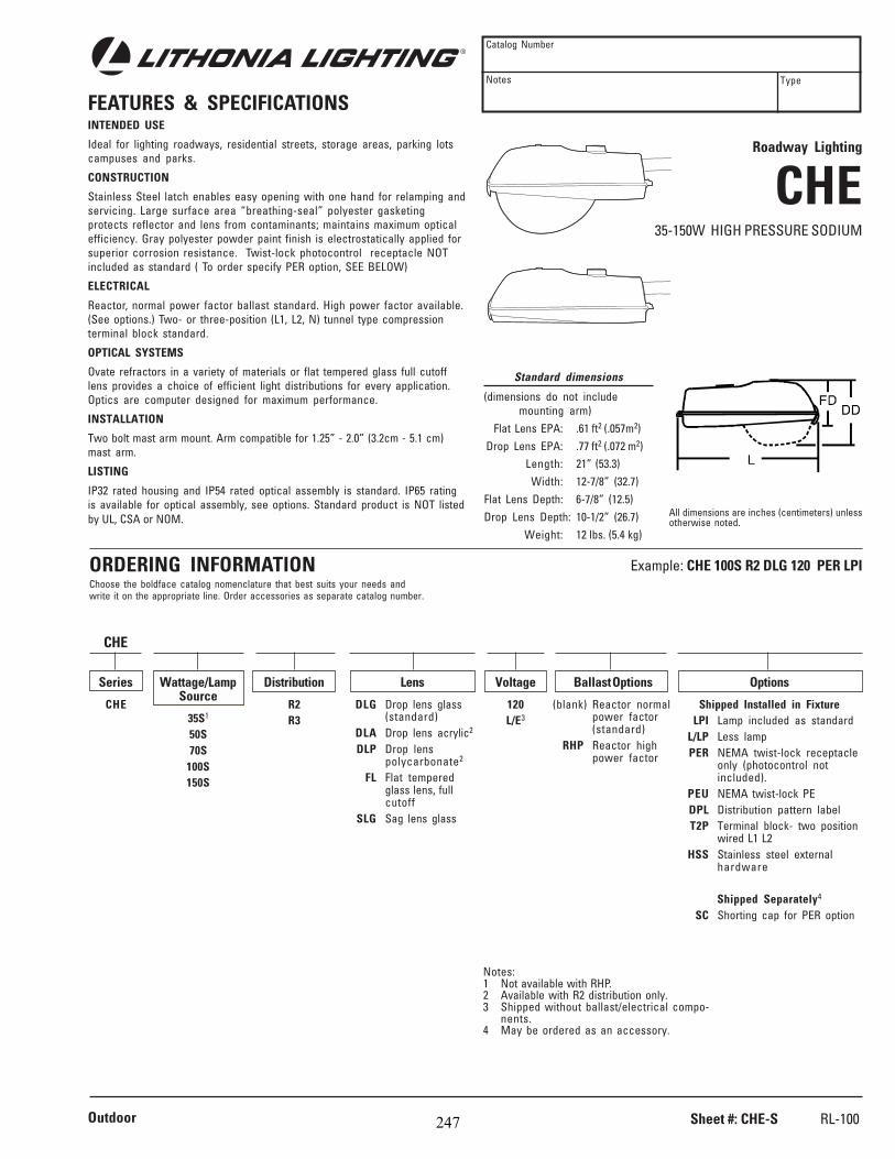
ORDERING INFORMATIONChoose the boldface catalog nomenclature that best suits your needs andwrite it on the appropriate line. Order accessories as separate catalog number.

Example: CHE 100S R2 DLG 120 PER LPI

FEATURES & SPECIFICATIONSINTENDED USE

Ideal for lighting roadways, residential streets, storage areas, parking lotscampuses and parks.

CONSTRUCTION

Stainless Steel latch enables easy opening with one hand for relamping andservicing. Large surface area “breathing-seal” polyester gasketingprotects reflector and lens from contaminants; maintains maximum opticalefficiency. Gray polyester powder paint finish is electrostatically applied forsuperior corrosion resistance. Twist-lock photocontrol receptacle NOTincluded as standard ( To order specify PER option, SEE BELOW)

ELECTRICAL

Reactor, normal power factor ballast standard. High power factor available.(See options.) Two- or three-position (L1, L2, N) tunnel type compressionterminal block standard.

OPTICAL SYSTEMS

Ovate refractors in a variety of materials or flat tempered glass full cutofflens provides a choice of efficient light distributions for every application.Optics are computer designed for maximum performance.

INSTALLATION

Two bolt mast arm mount. Arm compatible for 1.25” - 2.0” (3.2cm - 5.1 cm)mast arm.

LISTING

IP32 rated housing and IP54 rated optical assembly is standard. IP65 ratingis available for optical assembly, see options. Standard product is NOT listedby UL, CSA or NOM.

Series

CHE

Distribution

R2R3

Outdoor

Catalog Number

Notes Type

Standard dimensions

(dimensions do not includemounting arm)

Flat Lens EPA: .61 ft2 (.057m2)Drop Lens EPA: .77 ft2 (.072 m2)

Length: 21” (53.3)Width: 12-7/8” (32.7)

Flat Lens Depth: 6-7/8” (12.5)Drop Lens Depth: 10-1/2” (26.7)

Weight: 12 lbs. (5.4 kg)

Wattage/LampSource

35S1

50S70S

100S150S

Lens

DLG Drop lens glass(standard)

DLA Drop lens acrylic2

DLP Drop lenspolycarbonate2

FL Flat temperedglass lens, fullcutoff

SLG Sag lens glass

Voltage

120L/E3

Ballast Options

(blank) Reactor normalpower factor(standard)

RHP Reactor highpower factor

Options

Shipped Installed in FixtureLPI Lamp included as standard

L/LP Less lampPER NEMA twist-lock receptacle

only (photocontrol notincluded).

PEU NEMA twist-lock PEDPL Distribution pattern labelT2P Terminal block- two position

wired L1 L2HSS Stainless steel external

hardware

Shipped Separately4

SC Shorting cap for PER option

Notes:1 Not available with RHP.2 Available with R2 distribution only.3 Shipped without ballast/electrical compo-

nents.4 May be ordered as an accessory.

CHE

All dimensions are inches (centimeters) unlessotherwise noted.

Roadway Lighting

CHE35-150W HIGH PRESSURE SODIUM

Sheet #: CHE-S RL-100247

SPECIFICATION FEATURES

07/19/2007 10:13:38 AMConsult your representative for additional options and finishes.

Specifications and Dimensions subject to change without notice. ADH060543

WALL MOUNT DRILLING ARM MOUNT DRILLINGDIMENSIONS

DESCRIPTION

The Lumark Hammer's one-piece die-cast housing provides smooth,

clean-line aesthetics while ensuring watertight protection of the electrical

components. A computer-designed optical assembly delivers repeatable

photometrics in four beam patterns for maximum design flexibility. The

AIR/AIS mounting option provides contractor friendly, single shipment of

fixture with the arm-in-box.

Superior beam utilization and smooth distribution make the Hammer ideal

for parking areas, access roadways and other general offstreet area/site

lighting applications.

A ... LatchesSpring-loaded, die-cast latches

provide entry without tools.

B ... HousingWeather-resistant, one-piece

die-cast aluminum housing is

finished in dark bronze polyester

powder coat as standard. Optional

colors available. U.L. listed for wet

locations. CSA certified.

C ... ReflectorHydroformed anodized aluminum

reflector delivers repeatable Type I,

II, III and Forward Throw

distributions.

D ... GasketDie-cut, dacron polyester gasket

seals out external contaminants.

IP65 rated optical assembly.

E ... DoorRemovable one-piece die-cast

aluminum door with clear flat

tempered glass lens.

F ... SocketMogul-base porcelain socket for

high pressure sodium or above

150W Metal Halide lamps.

G ... BallastRemovable swing-down ballast

assembly standard on arm mount

units. Optional hard mount

available. Hard mount ballast

assembly standard on internal

slipfitter option.

HRHAMMER

70-400WHigh Pressure Sodium

Metal Halide

ARM-MOUNTED

AREA/SITE LUMINAIRE

248

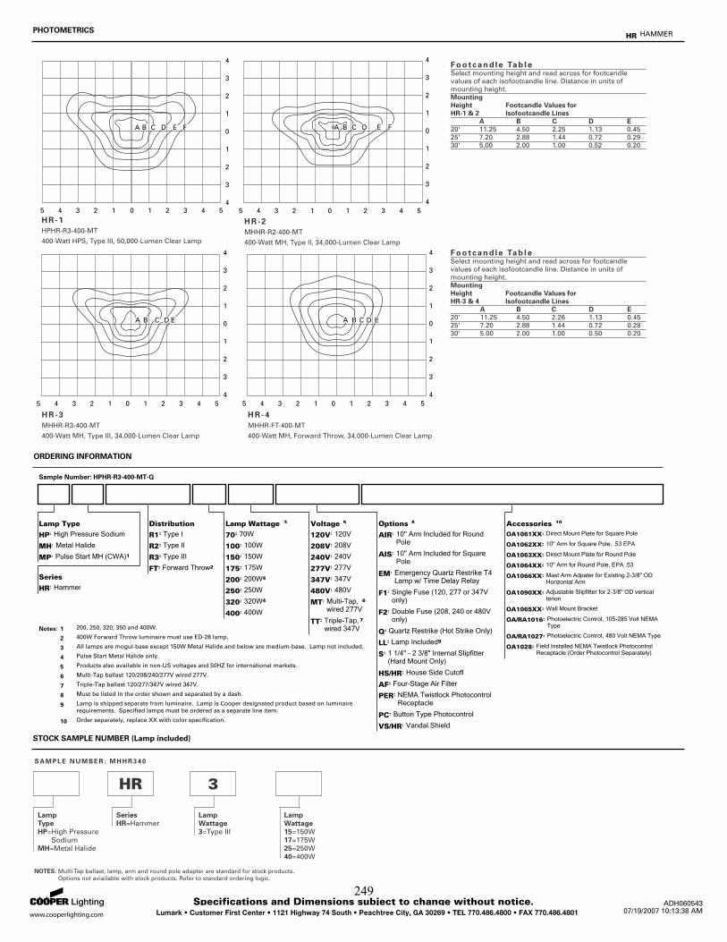
Lumark • Customer First Center • 1121 Highway 74 South • Peachtree City, GA 30269 • TEL 770.486.4800 • FAX 770.486.4801 07/19/2007 10:13:38 AM


PHOTOMETRICS

STOCK SAMPLE NUMBER (Lamp included)

HAMMERHR

ORDERING INFORMATION

Sample Number: HPHR-R3-400-MT-Q

Voltage 5

120V 120V=

208V 208V=

240V 240V=

277V 277V=

347V 347V=

480V 480V=

MT Multi-Tap,wired 277V

6=

TT Triple-Tap,wired 347V

7=

Options 8

AIR 10'' Arm Included for Round Pole

=

AIS 10'' Arm Included for Square Pole

=

EM Emergency Quartz Restrike T4 Lamp w/ Time Delay Relay

=

F1 Single Fuse (120, 277 or 347V only)

=

F2 Double Fuse (208, 240 or 480V only)

=

Q Quartz Restrike (Hot Strike Only)=

LL Lamp Included9=

S 1 1/4" - 2 3/8" Internal Slipfitter (Hard Mount Only)

=

HS/HR House Side Cutoff=

AF Four-Stage Air Filter=

PER NEMA Twistlock Photocontrol Receptacle

=

PC Button Type Photocontrol=

VS/HR Vandal Shield=

Accessories 10

OA1061XX Direct Mount Plate for Square Pole=

OA1062XX 10'' Arm for Square Pole, .53 EPA=

OA1063XX Direct Mount Plate for Round Pole=

OA1064XX 10'' Arm for Round Pole, EPA .53=

OA1066XX Mast Arm Adpater for Existing 2-3/8'' OD Horizontal Arm

=

OA1090XX Adjustable Slipfitter for 2-3/8'' OD vertical tenon

=

OA1065XX Wall Mount Bracket=

OA/RA1016 Photoelectric Control, 105-285 Volt NEMA Type

=

OA/RA1027 Photoelectric Control, 480 Volt NEMA Type=

OA1028 Field Installed NEMA Twistlock Photocontrol Receptacle (Order Photocontrol Separately)

=

Lamp Wattage 3

70 70W=

100 100W=

150 150W=

175 175W=

200 200W4=

250 250W=

320 320W4=

400 400W=

Lamp Type

HP High Pressure Sodium=

MH Metal Halide=

MP Pulse Start MH (CWA)1=

Distribution

R1 Type I=

R2 Type II=

R3 Type III=

FT Forward Throw2=Series

HR Hammer=

1 200, 250, 320, 350 and 400W.Notes:

2 400W Forward Throw luminaire must use ED-28 lamp.

3 All lamps are mogul-base except 150W Metal Halide and below are medium-base. Lamp not included.

4 Pulse Start Metal Halide only.

5 Products also available in non-US voltages and 50HZ for international markets.

6 Multi-Tap ballast 120/208/240/277V wired 277V.

7 Triple-Tap ballast 120/277/347V wired 347V.

8 Must be listed in the order shown and separated by a dash.

9 Lamp is shipped separate from luminaire. Lamp is Cooper designated product based on luminaire

requirements. Specified lamps must be ordered as a separate line item.

10 Order separately, replace XX with color specification.

249

SPECIFICATION FEATURES

05/03/2007 5:12:13 PMConsult your representative for additional options and finishes.


DIMENSIONS

DESCRIPTION

Roadway Cobrahead fixtures feature durable die-cast aluminum

construction and a computer-designed optical system for sturdiness and

optimum photometric control.

A ... HousingDie-cast aluminum housing and

integrally cast door hinge are

finished in durable grey polyester

powder coat.

B ... ReflectorThe reflector is precision

hydroformed anodized aluminum

with a Dacron polyester filter.

C ... DoorDie-cast aluminum door frame has

two-position latch to ensure door

stays fastened under extreme

conditions.

D ... LensRemovable prismatic refractor for

use with high pressure sodium and

metal halide lamp sources.

E ... SocketAdjustable mogul-base porcelain

socket.

F ... Ballast AssemblyHard mounted ballast with

encapsulated starter and plastic

terminal block for protection from

environmental abuse.

G ... MountingTwo-bolt/one clamp slipfitter for

1 1/4" or 2" mounting arms.

RYROADWAY

COBRAHEAD

50W-400WHigh Pressure Sodium

Metal Halide

SITE/ROADWAY LIGHT

250

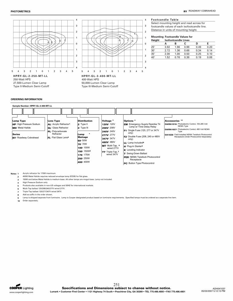
Lumark • Customer First Center • 1121 Highway 74 South • Peachtree City, GA 30269 • TEL 770.486.4800 • FAX 770.486.4801 05/03/2007 5:12:13 PM


PHOTOMETRICS ROADWAY COBRAHEADRY

ORDERING INFORMATION

Sample Number: HPRY-GL-3-400-MT-LL

Voltage 5

120V 120V=

208V 208V=

240V 240V=

277V 277V=

347V 347V=

480V 480V=

MT Multi-Tap,wired 277V

6=

TT Triple-Tap,wired 347V

7=

Options 8

EM Emergency Quartz Restrike T4 Lamp w/ Time Delay Relay

=

F1 Single Fuse (120, 277 or 347V only)

=

F2 Double Fuse (208, 240 or 480V only)

=

LL Lamp Included9=

H Plug-In Starter4=

K Leveling Indicator=

T Swing-Down Ballast=

PER NEMA Twistlock Photocontrol Receptacle

=

PC Button Type Photocontrol=

Accessories 10

OA/RA1016 Photoelectric Control, 105-285 Volt NEMA Type

=

OA/RA1027 Photoelectric Control, 480 Volt NEMA Type

=

OA1028 Field Installed NEMA Twistlock Photocontrol Receptacle (Order Photocontrol Separately)

=

Distribution

2 Type II=

3 Type III=

Lamp Type

HP High Pressure Sodium=

MH Metal Halide=

Lens Type

AL Acrylic Refractor1=

GL Glass Refractor=

PL PolycarbonateRefractor

=

FL Flat Glass Lens2=LampWattage

3

50 50W=

70 70W=

100 100W=

150 150W4=

175 175W=

250 250W=

400 400W=

Series

RY Roadway Cobrahead=

1 Acrylic refractor for 175W maximum.Notes:

2 400W Metal Halide requires reduced envelope lamp (ED28) for flat glass.

3 150W and below Metal Halide is medium-base. All other lamps are mogul-base. Lamp not included.

4 High Pressure Sodium only.

5 Products also available in non-US voltages and 50HZ for international markets.

6 Multi-Tap ballast 120/208/240/277V wired 277V.

7 Triple-Tap ballast 120/277/347V wired 347V.

8 Add as suffix in the order shown.

9 Lamp is shipped separate from luminaire. Lamp is Cooper designated product based on luminaire requirements. Specified lamps must be ordered as a separate line item.

10 Order separately.

251

Date:

Quote/Job no.:

Job Name:

Pole Specification:

Pole Logic:

POLE Height Above Grade 32 (ft)Shape RO (Pole Logic Code)Taper 15 (mm/m)

Tip Diameter 210 (mm)

FIXTURES Qty.: 1 (enter 0 if none)Height Above Grade (to centre) 9.7 (m)

EPA (each) 1 (ft2)

ARMS Qty.: 1 (enter 0 if none)Height Above Grade (to centre) 9.7 (m)

EPA (each) 0.6 (ft2)Arm Length 8 (ft)

BANNERS Qty.: 0 (enter 0 if none)Height Above Grade (to centre) 0 (m)

Length 0 (in)Width 0 (in)

WIND Speed (from map) 80 (mph)

Bending Force at 600mm from Tip 1.55 (kN)

Torsion Force 0.68 (kN-m)

Govering Design Class AA* (CSA)

Checked By Engineering:

New AAHSTO 2001 LOADSKz 1.09G 1.14V 80.57 180 mphIr 1 < 10 mCd 1

4944.859447 Pa

Tf-arm 0.55 kN-mTf-fixt 1.75 kN-m

2.30 kN-m0.4 kN-m for 80 mph1.84 kN-m for 160 mph

AA*

A

Pole Classification Based on Wind Load

(CSA)Torsional Class

Tranverse Class (CSA)

File Path: Z/Engineering/Designs/ Nov 17 2006 REV 000252

Torsion in Helically Reinforced Prestressed Concrete Poles

Documents