Toroid Cavity Detectors for High-Resolution NMR Spectroscopy and Rotating Frame Imaging: Capabilities and Limitations

Toroid Cavity Detectors for High-Resolution NMR Spectroscopy

and Rotating Frame Imaging: Capabilities and Limitations

Konstantin I. Momot, Nader Binesh, Olaf Kohlmann and Charles S. Johnson, Jr.*

Department of Chemistry, University of North Carolina, Chapel Hill, NC 27599-3290

* To whom correspondence should be addressed.

Corresponding author: Charles S. Johnson, Jr.

Voice: (919) 966-5229

FAX: (919) 962-2388

EMAIL: [email protected]

Running Title: Toroid Cavity Detectors

Momot, Konstantin I. and Binesh, Nader and Kohlmann, Olaf and Johnson, Jr., Charles S.

(2000) Toroid Cavity Detectors for High-Resolution NMR Spectroscopy and Rotating

Frame Imaging: Capabilities and Limitations. Journal of Magnetic Resonance 142(2):pp.

348-357.

Copyright 2000 Elsevier

−2−

ABSTRACT

The capabilities of toroid cavity detectors for simultaneous rotating frame imaging

and NMR spectroscopy have been investigated by means of experiments and computer

simulations. The following problems are described: (a) magnetic field inhomogeneity and

subsequent loss of chemical shift resolution resulting from bulk magnetic susceptibility

effects, (b) image distortions resulting from off-resonance excitation and saturation effects,

and (c) distortion of line shapes and images resulting from radiation damping. Also, special

features of signal analysis including truncation effects and the propagation of noise are

discussed. Bo inhomogeneity resulting from susceptibility mismatch is a serious problem

for applications requiring high spectral resolution. Image distortions resulting from off-

resonance excitation are not serious within the rather narrow spectral range permitted by

the RF pulse lengths required to read out the image. Incomplete relaxation effects are

easily recognized and can be avoided. Also, radiation damping produces unexpectedly

small effects because of self-cancellation of magnetization and short free induction decay

times. The results are encouraging, but with present designs only modest spectral

resolution can be achieved.

Keywords: toroid, imaging, rotating frame, radiation damping, diffusion

−3−

Introduction

Radiofrequency (RF) fields for NMR spectroscopy are usually provided by solenoid

or saddle coils. In high-resolution applications, uniformity of B1 fields and sensitivity are

highly desirable, but the choice of coil type is usually dictated by the magnet geometry and

spatial restrictions. For example, NMR in superconducting magnets requires that the RF

field be polarized perpendicular to the vertical symmetry axis of the magnet. Saddle coils

that can accommodate vertical sample tubes are often chosen in spite of the fact that the

signal to noise (S/N) ratio is expected to be a factor of three lower than for solenoid coils

(1). The S/N difference results largely from the lower filling factors for samples in saddle

coils that is associated with the inefficient use of the flux density. A way around this

problem, when high sensitivity is required, is to use a toroid coil than can efficiently trap the

flux and provide reasonable B1 homogeneity. In fact, toroid coils have been shown to give

S/N enhancements of a factor of four or better relative to saddle coils, but at the cost of

sample handling inconvenience and a small flux cross-section compared with the horizontal

space required for the coil (2,3).

There are, of course, very different requirements for RF field gradient spectroscopy.

Imaging applications and diffusion measurements require constant B1 gradients or at least

that the amplitude of the RF field be simply related to the spatial position (4). The

combination of RF gradients with high-resolution NMR typically involves the use of a single

loop transmitter coil, to provide the RF gradient, with a saddle coil for homogeneous B1

pulses and for detection (5). This arrangement has been successfully used for NMR

microscopy and for diffusion measurements but is limited in the magnitude of gradients that

can be produced and the extent of the region where the gradient is approximately constant.

Cylindrical NMR detectors similar to that illustrated in Fig. 1 have some of the

−4−

properties of toroid coils and provide well characterized RF gradients (6). These devices,

known as toroid cavity detectors (TCDs), behave as a continuous array of single loops

connected in parallel in contrast to the toroid coils where the loops are in series. The TCD

is, thus, a low inductance device that can be tuned to relatively high frequencies.

Furthermore, the amplitude of the RF field is inversely proportional to the distance from the

symmetry axis of the cavity. It is interesting to note that the first successful NMR

experiment on bulk matter made use of a TCD (7,8).

FIGURE 1

The following advantages of TCDs have been emphasized: (a) sensitivity is inversely

proportional to r (reciprocity principle)(1) thus permitting the detection of signals from thin

layers close to the central rod (9), (b) rotating frame imaging of spin densities and

displacements with respect to r is practical and provides high resolution (~20 µm) for small

values of r (10), (c) TCDs can serve as cells for high pressure NMR, and (d) the central rod

can be electrically isolated from ground so it can serve as an electrode in electrochemistry

experiments (6). What has not been demonstrated or even claimed is that rotating frame

imaging with TCDs is compatible with high-resolution NMR.

Since we are interested in chemical applications of TCDs that require both chemical

shift resolution and the determination of molecular displacement by means of imaging, we

have undertaken experiments and computer simulations to investigate the characteristics of

these detectors. In this paper we explore the following problems: (a) reduced chemical shift

resolution resulting from bulk magnetic susceptibility effects, (b) image distortions resulting

from off-resonance excitation and saturation effects, and (c) distortion of line shapes and

images resulting from radiation damping. To anticipate the results, we find that Bo

inhomogeneity resulting from susceptibility mismatch is indeed a serious problem that

−5−

cannot be eliminated without changing the geometry of the TCD or possibly by using

specialized shim stacks. Characteristic image distortions resulting from off-resonance

excitation have been obtained both experimentally and theoretically, and fortunately are not

serious within the rather narrow spectral range permitted by the RF pulse lengths required

to read out the image. Also, saturation or incomplete relaxation effects produce image

distortions with an easily recognized signature that can be avoided by reducing the

repetition rate of the experiment. The predicted effect of radiation damping in experiments

involving magnetization gratings consists primarily of winding or unwinding the

magnetization helix after the RF preparation pulse; however, this effect was too small to be

detected experimentally. In general the results are encouraging, but with present

technology one must be satisfied with modest spectral resolution.

Background

RF fields inside TCDs: The TCD is essentially a small copper can with a central conductor

insulated from one end and making contact with the other as shown in Fig. 1, i.e. a co-axial

detector. The RF field amplitude in the cavity is given by B1 = A/r where A is the toroid

constant, sometimes called the A factor, and r is the distance from the symmetry axis. This

permits precisely known phase encoding of the radial position, i.e. an RF pulse produces a

Saarinen helix with a pitch proportional to r2 (11). It should be noted that the oscillating RF

field is tangential to the circular field lines shown in Fig. 1. At any point we choose the

laboratory coordinate frame so that the X-axis is also tangential to the field lines and the Y-

axis is in the radial direction. As with conventional RF coils, the oscillating field is resolved

into counterrotating components and only the one rotating with the same sense as the

nuclei of interest is retained. The rotating B1 field then defines the x-axis in the rotating

frame. Only the rotating coordinate systems with origins in the same radial direction have

−6−

the same orientation relative to the laboratory frame at a given time. Fortunately, the array

of orientations does not introduce any complications in the analysis since the relative

orientations of fields and isochromats are identical in all rotating coordinate systems with

origins at the same distance from the symmetry axis, i.e. the same value of r.

Imaging with TCDs: The rotating frame imaging (RFI) method makes use of RF field

gradients to encode nuclear positions (4). Woelk, et al., have applied this technique to

obtain radial images of samples in TCDs (9). They have also demonstrated the use of the

magnetization grid rotating frame imaging (MAGROFI) method (12) to image diffusion in

TCDs (10). The situation with RFI and MAGROFI differs from pulsed field gradient (PFG)

NMR because the RF pulses both excite the spins and provide the radial gradient for

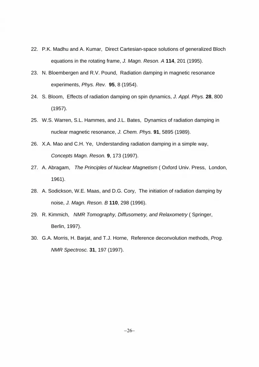
imaging. In MAGROFI (Fig. 2) the first pulse, of length tP1, generates a z-magnetization

pattern (after transverse components are eliminated) that is proportional to cos[q(r)r] where

q(r) = γAtP1/r2, thus covering all q space in a single shot. The second RF pulse is

incremented in n steps of ∆tP2, i.e. tP2 = n∆tP2 with n = 0 to N-1, in order to obtain NMR

signals with information that characterizes the magnetization pattern or grid present at the

end of the diffusion period τ. If tP1 is set equal to zero, the second pulse simply images the

spin density of the sample as in the RFI experiment.

FIGURE 2

The free induction decay (FID) obtained for each value of tP2 is Fourier transformed

with respect to time to obtain the amplitude of the (absorption mode) signal of interest. The

signal amplitude versus pulse length, i.e. the interferogram, can be expressed as (13):

max

min

sinr P2

z P1P2

r

tS ( ) = t tM

A 1(r, + ) 2 rh drr r

γτ π⎛ ⎞ ⋅ ⋅∫ ⎜ ⎟⎝ ⎠

−7−

Here Mz(r, tP1+τ) is magnitude of the z-component of magnetization of the nuclei of interest

at the beginning of the pulse P2. Equation [1] represents the transverse component of

magnetization integrated over the volume of the sample, here assumed to fill the TCD,

taking into account the inverse dependence of sensitivity on radius. Since the precession

frequency of spins in the RF field is given by ω1 = γA/r, the transformation of variables (r to

ω1) permits Eq. [1] to be recognized as the sine Fourier transform of r2Mz(r, tP1+τ). The

image of Mz(r, tP1+τ) can thus be obtained by dividing the inverse sine transform of S(tP2) by

r2.

Effects of radial diffusion and flow: The magnetization grid, that is a simple cosinusoidal

function of 1/r at the end of the first RF pulse, is modified by diffusion, flow, and longitudinal

relaxation during the diffusion interval τ. At time tP1+ τ the magnetization at position r is

described by (14):

In Eq. [2] D is the tracer diffusion coefficient, v(r) is the position dependent radial velocity,

and T1 is the longitudinal relaxation time. We note that q(r) = 2π/Λ(r) where Λ(r) is the local

period or wavelength of the grid. Therefore, the scattering vector q(r) is the local tightness

of the grid and is responsible for sensitizing the sample to diffusion and flow.

Experimental Section

Probes for TCD experiments: The basic principles of design of TCDs have been described

in the literature (6). The TCD used in this work was made of beryllium-copper alloy except

for the central rod which was copper. The dimensions defined in Fig. 1 were as follows: rmin

( ){ }exp cos exp2z 0

1

(r) = 1 - 1 - -D q(r [q(r)(r + v(r) )] - )M MTττ τ

⎡ ⎤⎛ ⎞⎢ ⎥⎜ ⎟

⎝ ⎠⎣ ⎦

−8−

= 0.8 mm; rmax = 7.4 mm; h = 24 mm, wall thickness = 2 mm, and outside height = 30 mm.

In anticipation of future use of the TCD in electrophoresis experiments, all interior surfaces

were electroplated with silver and the copper rod was isolated from ground by placing two

chip capacitors (that were part of the resonance circuit) on top of the TCD. It was found

that the arrangement of these capacitors affects the lineshape and achievable shimming

quality. Trimmers, required for tuning and matching, were placed as close to the TCD as

possible to minimize the stray inductance.

To reduce the effects of susceptibility mismatch, top/bottom inserts were placed

inside the cavity. The inserts were 3 mm thick disks machined from PEEK (χ = -9.3 ppm)

(15). In some of the test experiments, sample inserts were also introduced to constrain the

sample volume (concentric inserts). The inserts were machined of Teflon (χ = -10.5 ppm)

or PEEK and typically the radial thickness was 2 to 5 mm.

NMR Samples and Spectra: 1H spectra were obtained with H2O/D2O samples having

compositions ranging from 1 % to 50 % H2O. D2O (99.9 atom % D) was obtained from

Aldrich Chemical Co., and distilled water was added to prepare the required ratios of

H2O/D2O.

Image acquisition rates were severely limited by the T1s of the HDO proton, and

relaxation delays of 30 to 60 s were typically required. Copper sulfate(1 mM) was

sometimes added to the solutions as a relaxation agent to shorten the T1 of HDO to

approximately 1 s (16).

Spectrometer requirements: For imaging applications it is required that the toroid constant

A be of the order of 1 mT⋅mm and that the RF pulse amplitudes remain constant up to 5

ms. All spectra in this work were acquired on a Bruker AC250 spectrometer with a Tecmag

−9−

computer upgrade. The original RF amplifier provided a maximum of only 30W and the

power output drooped significantly after about 100 µs. These limitations were circumvented

by using the low power output (800 mW) from the Bruker amplifier through a set of

attenuators to drive a 150 W power amplifier (AMT M3135). This arrangement provided

power stability of better than 1% for 10 ms. The input to the power amplifier was limited to

0.1 mW with a maximum duration of 20 ms by a homemade protection circuit which in turn

limited the output power of the amplifier to 40 W to avoid overloading the Bruker RF

preamplifier. Fortunately, this level was sufficient to provide an average A factor of

1 mT⋅mm.

Experimental parameters and data analysis: RF imaging places severe restrictions on the

choices of pulse lengths. Consider the problem of imaging a z-magnetization pattern

created by an RF pulse of duration tP1 and having the form cos[q(r)r]. We must consider

both foldover and digital resolution (17). According to the Nyquist theorem we must sample

at least two times in each period in the pattern to avoid foldover. Therefore, we require that

To calculate the spatial resolution, we note that in the frequency domain δv = 1/tP2 where

v = ω1/(2π). Then by using the relationship δv = (γA/2πr2)δr, we find that the resolution is

given by

Eqs. [3] and [4] can be combined with r ≈ rmin to obtain a lower limit on digital resolution

close to the rod, δr ≥ 2rmin/n. If the resolution is selected to be Λ(r)/2, Eq. [4] indicates that

tP2 = 2tP1. Digital resolution can, of course, be improved by means of “zero-filling” the

interferogram prior to the Fourier transformation (17).

minP2

r < tA

πγ

∆

2

P2

2 rr = An tπδ

γ ∆

−10−

Taking into account these restrictions, a typical experiment with A = 1.0 mT⋅ mm

might have ∆tP2 = 4 µs and N = 256. This combination yields tP2(max) = 1 ms which yields

an effective spectral width of the order of 1 kHz. The effects of resonance offset on images

are presented in Results and Discussion.

The experimental toroid factor A can be determined from an interferogram obtained

with tP1 = 0. A satisfactory procedure is to use the Levenberg-Marquardt algorithm (18) to

obtain a least squares fit of the experimental interferogram to the right hand side of Eq. [1]

with τ = 0. The amplitude and baseline of the interferogram can be included in the fitted

parameters. However, the least squares determination of rmin and rmax is unstable. These

parameters should be measured independently and not determined by the fitting procedure.

Another experimental problem is that interferograms often must be truncated, and

the way this is done affects the quality of the image. As a general rule, truncating the

interferogram at a node, S(tp2max)=0, is beneficial to the image quality. Also, two-fold zero-

filling of a non-zero terminated interferogram produces significant "beats" in image

amplitude, while analogous zero-filling of a zero-terminated interferogram preserves the

overall quality of the image. Truncation effects are usually less severe in cases where

interferograms rapidly decay to zero, e.g. imaging of gratings.

The simulations reported here were performed on a Dell 350 MHz Pentium II PC

using the software packages Digital Fortran, Mathcad, and Mathematica.

Results and Discussion

In RFI the “ideal” interferogram described by Eq. [1] is obtained when RF excitation

is the only factor considered. However, in real NMR experiments, factors that distort the

interferogram must be taken into account, e.g. inhomogeneity of the static field inside the

−11−

sample, resonance offset, relaxation, and radiation damping. The effects of these factors

on the image and their experimental "signatures" are discussed in this section.

The simulations presented here are based on the Bloch equations. Unless noted

otherwise, NMR experiments were simulated in the following way. The rotating frame (x-

axis defined by B1) was on resonance and the RF pulses were simulated by simple

rotations. During the pulses relaxation, radiation damping, and diffusion were neglected.

The free evolution periods were modeled by solving Bloch equations that included any or all

of the following: precession in the effective local field, relaxation, diffusion, and radiation

damping. Diffusion was modeled using the diffusion propagator (10). Each point of the FID

was obtained by integrating the transverse magnetization over the volume of the toroid

cavity, and in the construction of an interferogram, only the absorptive part of the Fourier

transformed FID was used.

In some of the simulations uniform uncorrelated Gaussian noise (18) was added to

the simulated interferogram. The RMS noise, defined as a percentage of the maximum

interferogram intensity, was typically 0.5 % to 1 %. In the image, the noise amplitude is

proportional to 1/r2 because of the required division by r2 after Fourier Transformation. It

should be noted that 0.5 % noise in the interferogram noise transforms to 10% - 20% image

noise at rmin and negligible noise at rmax, in agreement with experimentally observed

images.

Intrinsic B0 inhomogeneity: When a sample with non-zero magnetic susceptibility is placed

in a homogeneous magnetic field, the field inside the sample is inhomogeneous for most

sample geometries. This “intrinsic” inhomogeneity is thus a characteristic of the sample

and its enclosure. For samples in TCDs we have computed the internal distribution of field

by means of the magnetization surface currents approach (15,19).

−12−

If the TCD and sample are represented by a number of blocks of uniform materials

(sample, metal, susceptibility matching plugs), the induced component of the magnetic field

can be calculated with Biot-Savart law as shown in Eq. [5]:

where S i is the surface of interface i, (∆χ)i is the susceptibility difference at interface i, ei is

a unit vector tangential to the surface of interface i and perpendicular to B0, and d2r' spans

Si. In cylindrical coordinates the surface element d2r' takes the form Ri(z)dφdz where Ri(z)

is the radius of interface i in cylindrical coordinates and r' specifies the point [Ri(z), φ, z].

Computationally, various geometries of susceptibility matching plugs can be incorporated in

a modular fashion by creating for each interface a subroutine defining its geometry

("surface definition subroutine") and later calling the surface current integration subroutine

with the name of the respective surface definition subroutine as a parameter. This

approach has been implemented in a Digital FORTRAN program named Toroid_MAP.

Numerical integration of Eq. [5] for the TCD described in the Experimental Section

yields the field map for a grid of points in the (r,z) plane that is illustrated in Fig. 3. An

analysis of the B(r) components shows an inhomogeneous distribution of radial and axial

components throughout the sample volume. For a D2O sample, representative values of

the quantities describing the induced part of B(r) are the following: <Bz> = 1850 Hz, relative

standard deviation σ(<Bz>) = 0.12, absolute standard deviation σ(<Br>) = 1400 Hz, with B

expressed in terms of the 1H precession frequency at 5.87 T. The axial components Br(r)

can be neglected in the presence of a large applied field, even though their magnitude has

i

0 ii

0 20 3

i S

( )B ( - )( ) = rd4 | - |

χµµ

π

⎡ ⎤∆ ′×⎢ ⎥⎣ ⎦ ′

′∑ ∫r re

B rr r

−13−

the same order as inhomogeneity of the axial component.

FIGURE 3

When a TCD is used to obtain an NMR spectrum, an RF pulse first generates a

pattern of transverse magnetization components throughout the sample. In the presence of

intrinsic inhomogeneity the FID depends on the amount of transverse magnetization

associated with each value of the local magnetic field. Therefore, the FID and the resulting

line shape depend on both the duration of the RF pulse and the distribution of static fields.

The simulations presented here permit the NMR line shape for a particular TCD and

sample to be obtained as a function of the RF pulse length. The complete simulation

requires the convolution of the weighted frequency distribution with a Lorentzian function

having the appropriate T2 value. In the interest of computational efficiency we have chosen

to approximate the distribution of local frequencies with a polynomial expansion prior to the

convolution.

We note that the cylindrically symmetric Bz(r) distribution can be represented

analytically by a set of gradients containing even powers of z and all powers of r. Such an

expansion can be performed using, among other methods, the generalized least squares

approach (18). In this work, we used the direct product of {1, r, ... r4} and {1, z2, ... z10} as

the basis set for expanding the TCD field maps. This basis set provides good numerical

accuracy (RMS < 0.7 Hz) and is sufficiently compact to be practical in lineshape

calculations. The expansion of Bz(r) shows that the most important gradients describing its

inhomogeneity are +r2 and -z2.

The simulated lineshape is essentially a histogram of local magnetic fields weighted

by the local transverse magnetization density and convoluted with a Lorentzian shape

−14−

function. Figure 4a shows the lineshape simulated for an unshimmed H2O/D2O (1:99)

sample acquired with a 4 µs RF pulse (A = 1.0 mT⋅mm, T2 = 1.0 s). The inhomogeneity of

Bz(r) gives rise to an unsymmetric lineshape with widths at half-height and 0.1 height of

∆v0.5 = 20 Hz and ∆v0.1 = 330 Hz, respectively. Experimentally recorded spectra of

unshimmed samples have comparable linewidths, although direct comparison is

problematic because of uncertainty as to what set of shims produces a "perfectly

homogeneous external field." Unfortunately, the lineshape deteriorates markedly with

increasing pulse length.

FIGURE 4

In view of the successful fitting of Bz(r) with an extensive set of gradients, we

undertook the determination of the limits of shimming with known shim functions. The

"simulated shimming" procedure is similar to the least squares expansion of a TCD field

map with the following differences. Since the available shim gradients are not cylindrically

symmetric, a 3D field map must be constructed from the original 2D field map. Axial

symmetry is maintained in the shimmed field distribution only through the effect of

combinations of gradients on the 3D map.

The map of the "shimmed" field is given by the residues of the least squares fitting

procedure. This procedure determines the best possible shimming with our spectrometer

because the basis set contains only the standard set of shim gradients of a Bruker AC250

instrument (which includes all except the last 4 gradients listed in Table 2.1, reference

(20)). The unshimmed and shimmed lineshapes are shown in Figs. 4a and 4b,

respectively, with different frequency scales. The solid line in Figure 4b shows the

theoretical limit of the shimming corresponding to the global minimum of χ2 in the least

−15−

squares procedure. This lineshape has the width at half-height of ∆v0.5 = 8 Hz and at 0.1

height of ∆v0.1 = 20 Hz. The dashed line is a result obtained with slightly mismatched

shims. The latter spectrum features a narrow central component with wide inhomogeneous

"wings" - an observation described previously in the literature (13).

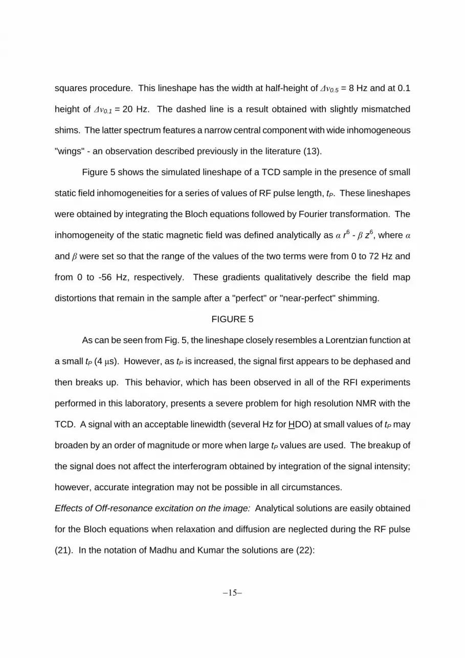
Figure 5 shows the simulated lineshape of a TCD sample in the presence of small

static field inhomogeneities for a series of values of RF pulse length, tP. These lineshapes

were obtained by integrating the Bloch equations followed by Fourier transformation. The

inhomogeneity of the static magnetic field was defined analytically as α r6 - β z6, where α

and β were set so that the range of the values of the two terms were from 0 to 72 Hz and

from 0 to -56 Hz, respectively. These gradients qualitatively describe the field map

distortions that remain in the sample after a "perfect" or "near-perfect" shimming.

FIGURE 5

As can be seen from Fig. 5, the lineshape closely resembles a Lorentzian function at

a small tP (4 µs). However, as tP is increased, the signal first appears to be dephased and

then breaks up. This behavior, which has been observed in all of the RFI experiments

performed in this laboratory, presents a severe problem for high resolution NMR with the

TCD. A signal with an acceptable linewidth (several Hz for HDO) at small values of tP may

broaden by an order of magnitude or more when large tP values are used. The breakup of

the signal does not affect the interferogram obtained by integration of the signal intensity;

however, accurate integration may not be possible in all circumstances.

Effects of Off-resonance excitation on the image: Analytical solutions are easily obtained

for the Bloch equations when relaxation and diffusion are neglected during the RF pulse

(21). In the notation of Madhu and Kumar the solutions are (22):

−16−

where tanθe = δ/ω1, ωe = (ω12 + δ2 )1/2, ω1 = γB1, δ = γB0 - ω, and ω is the angular frequency

of the rotating coordinate system. For a sample in a TCD, Eq. [6] describes the precession

of the magnetization (at a particular radial position r) in a cone around the effective

magnetic field Heff = (A/r)i + (δ/γ)k. Since the angle between Heff and the z-axis decreases

as r increases, there are nonlinear changes in the amplitude and phase of My and a

resulting distortion in the image.

An interferogram obtained off-resonance is given by:

This equation permits the criteria for off-resonance distortion to be established. In the limit

of small offset, the radical in the denominator can be expanded to obtain the following

condition for accurate amplitude: rmaxδ/(γA) << 1. The second criterion, resulting from the

expansion of the radical in the argument of the sine function, reduces to δ < 2π/tP2, a

criterion already imposed by spectral width restrictions.

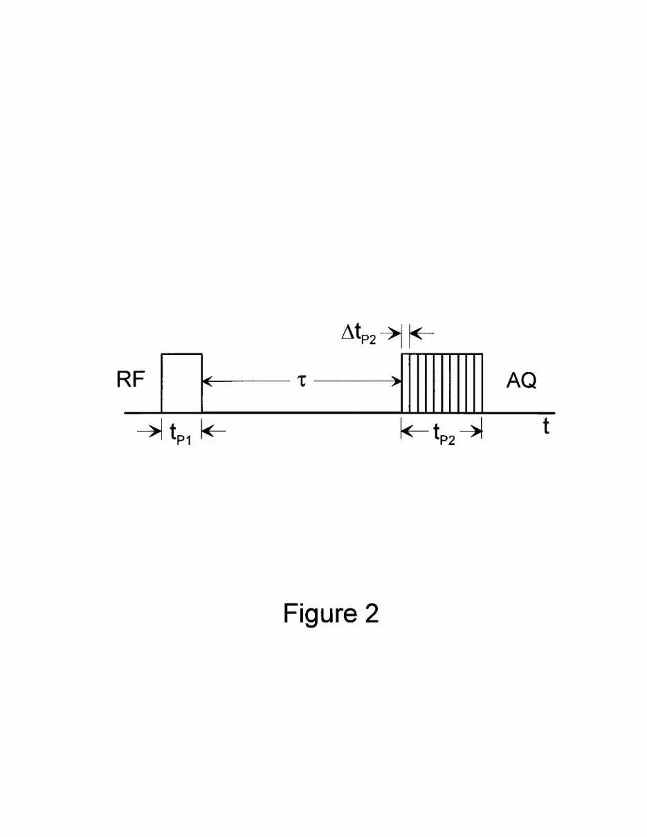
Experimental and simulated images obtained with offset frequencies ranging from 0

to 5 kHz are shown in Figs. 6a and 6b, respectively. There is good agreement between

these results, and we note that the parabolically rising roof of the image and the

underestimation of rmax are experimental signatures of off-resonance irradiation. The

retraction or shrinkage of the image is a consequence of the increase in precession

( )

sin sin

cos sin

cos sin

2x 0 e e

y 0 e e

2 2z 0 e e

= (2 ) ( t /2)M M

= ( ) ( t )M M

= 1 - 2 ( ) t M M

θ ω

θ ω

θ ω⎡ ⎤⎣ ⎦

max

min

sinr

2Py P 2

r

1 A 2t ( 2 ) = 2 h [ 1 + (r / A ] d r)S tr1 + (r / A )

γπ δ γδ γ

∫

−17−

frequency that results from the contribution of the offset term to Heff. An inspection of the

phase angle in Eq. [7] shows that the effective value of rmax becomes rmax/[1+(rmaxδ/γA)2]1/2.

The fractional increase is significant for larger values of r and results in mapping of the

intensity to lower r values in the image. This becomes apparent after introducing a new

integration variable, l = r/[1+(rδ/γA)2]1/2, and evaluating the new differential. For

(rδ/γA)2 << 1, the intensity of the image behaves as 1+(rδ/γA)2.

FIGURE 6

A hidden danger regarding determination of the toroid constant A from off-resonance

images should be noted. The A factor serves as a scaling factor for the r domain. Because

the apparent rmax is underestimated in off-resonance images, the A factor based on such

images will be overestimated in the least squares procedure mentioned in the Experimental

Section. Therefore, interferograms obtained on or near resonance must be used to

determine A unless the analysis is based on Eq. [7].

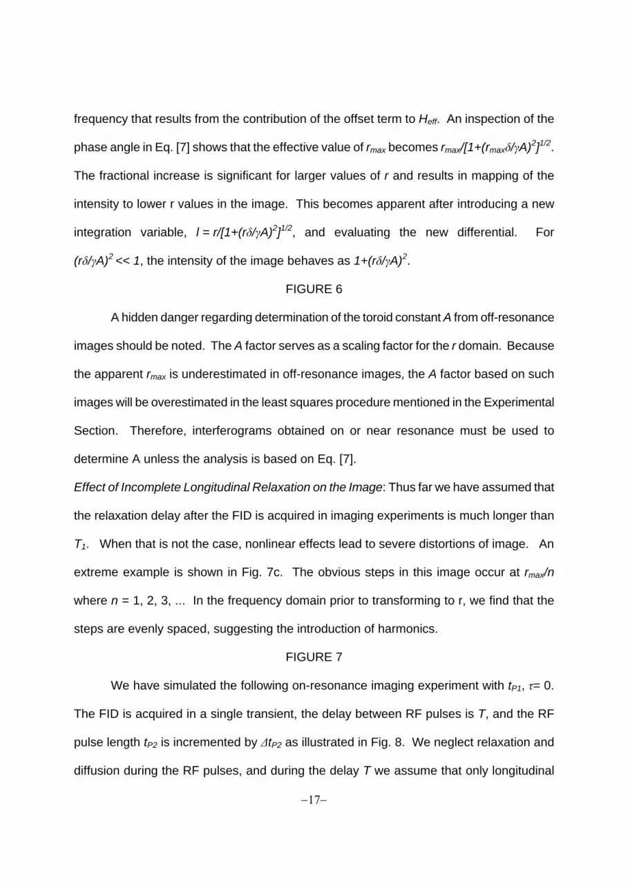
Effect of Incomplete Longitudinal Relaxation on the Image: Thus far we have assumed that

the relaxation delay after the FID is acquired in imaging experiments is much longer than

T1. When that is not the case, nonlinear effects lead to severe distortions of image. An

extreme example is shown in Fig. 7c. The obvious steps in this image occur at rmax/n

where n = 1, 2, 3, ... In the frequency domain prior to transforming to r, we find that the

steps are evenly spaced, suggesting the introduction of harmonics.

FIGURE 7

We have simulated the following on-resonance imaging experiment with tP1, τ= 0.

The FID is acquired in a single transient, the delay between RF pulses is T, and the RF

pulse length tP2 is incremented by ∆tP2 as illustrated in Fig. 8. We neglect relaxation and

diffusion during the RF pulses, and during the delay T we assume that only longitudinal

−18−

relaxation and diffusion are important. The nth RF pulse (P2) has the duration n∆tP2, and

we define the r dependent wavevector at the end of the nth pulse as qn(r) = γA n∆tP2/r2 so

that the phase angle resulting from the nth pulse is qn(r)r. The cumulative effect of

relaxation and diffusion on the acquired signals in this experiment on a sample with uniform

magnetization M0 can be described by the following iterative scheme (10,12):

FIGURE 8

We interpret Eqs. [8] as follows. The first RF pulse prepares a magnetization helix,

the transverse components of which contribute to an FID that provides the first point in the

interferogram. A z-magnetization pattern is also prepared; and, if T is not much larger that

T1, a residual pattern remains at the beginning of the second RF pulse. The residual

pattern is propagated by successive RF pulses as shown by the function fn(r), and the

points of the interferogram are given by:

The resulting interferogram suffers nonlinear but periodic distortions since the rate of

recovery of magnetization after an RF pulse depends on the deviation from the equilibrium

value. An image simulated with recursive scheme [8] with T/T1 = 1.0 is shown in Fig. 7f. In

general the effects of diffusion and transverse relaxation (during T) on the image are not

significant.

cos exp

exp

00

2n n n

0 0 1n+1n+1 n

(r) = f M

(r) = [ (r) r ] [-D (r)T ]q qC

(r) = + [ (r ) (r ) - ] (-T/ )f f CM M T

⋅

max

minsinr

n n-1 nr = 2 h (r) [ (r) r ] drf qS π ⋅∫

−19−

The experimental signature of incomplete longitudinal relaxation is the appearance

of descending "steps" in the image. At T/T1 = 5, the steps are negligibly small compared to

the image intensity while at T/T1 < 1, the steps are profound. We find that the number of

distinguishable steps ranges from 1 (2 < T/T1 < 5) to 3 (T/T1 < 1).

Radiation Damping: Effects of radiation damping on NMR signal have been studied

extensively for the solenoid and saddle coil detectors (23-27). The essence of the effect is

that the FID current in the detector coil induces the feedback magnetic field, Brd, that

oscillates with the precession frequency of the spins but has a π/2 phase delay. Interaction

of the magnetic moment of the spins with the feedback field leads to the radiation damping

term in the Bloch equations:

The explicit form of the damping term can be derived by the approach of Bloom

(24). After a RF pulse of length tP1, the current induced in the circuit is proportional to the

precessing magnetization or FID. On resonance and considering only radiation damping

effects we have:

where k is a proportionality constant and θ(r,0) = γAtP1/r. The effective B1 field resulting

from radiation damping is proportional to -FID(t)/r; and since FID(0) can be either positive

or negative this field acts to wind or unwind the magnetization helix created by the winding

pulse (P1) in the MAGROFI experiment. The winding or unwinding proceeds until the

FID(t) reaches the node of the interferogram nearest to the starting point in the indicated

rd

= [ ]d t

d γ⎛ ⎞

×⎜ ⎟⎝ ⎠

rdM M B

sin2

1

r

r0

2 1

(r, t) drFID(t) = k M - r r

θ∫

−20−

direction.

In a saddle coil detector, where the RF power is approximately uniform, radiation

damping drives magnetization to the thermal equilibrium at every point in the sample. The

uniformity of magnetization allows one to view radiation damping as being driven by local

transverse magnetization rather than by the FID. This approximation is reflected in the

commonly cited form of radiation damping terms of the Bloch equations (25,26), but is

invalid for TCDs because the RF field is not uniform. As a result, the magnetization at any

given point of the TCD can be driven past thermal equilibrium.

Another particularity of radiation damping in the TCD is the stability of Eq. [10] with a

vanishing initial FID. With a saddle coil or solenoid coil radiation damping is present

following a "perfect" π pulse because of the FID generated by thermal noise (26,28).

Therefore, inverted magnetization is unstable in the presence of radiation damping. This

situation is absent in the TCD since any node of the FID constitutes a stable point. Finally,

with the same sample and the same detector, a tight grating will be affected by radiation

damping to a lesser extent than a loose grating because the FID is essentially self-

canceling for tight gratings. Here the “tightness’ of a grating refers to the number of periods

of oscillation occurring between rmin and rmax, a number proportional to γAtP1. These

observations apply not only to the TCDs, but to any RFI detector (5,29).

In order to assess the effects of radiation damping on spectra and images obtained

with TCDs, we have performed two experiments. In the first experiment, spectra were

recorded for a series of H2O/D2O mixtures with compositions ranging from 1% to 50%

H2O in D2O. Each spectrum was recorded with a 4 µs RF pulse (A ≈ 1 mT⋅mm), and the

linewidth of the HDO signal was measured. All widths were in the range 7±1 Hz and no

−21−

significant correlation was found between the linewidth and concentration of H2O.

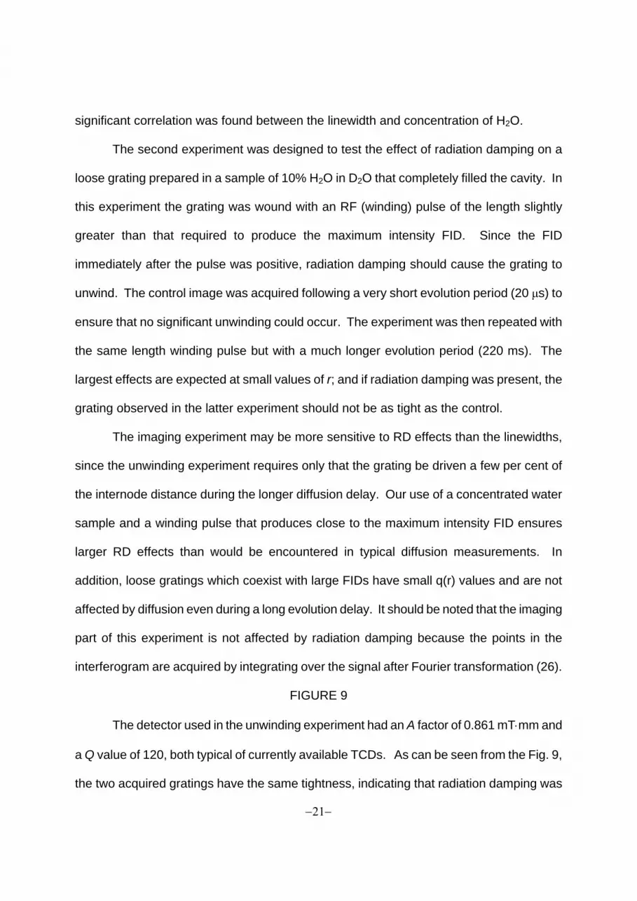
The second experiment was designed to test the effect of radiation damping on a

loose grating prepared in a sample of 10% H2O in D2O that completely filled the cavity. In

this experiment the grating was wound with an RF (winding) pulse of the length slightly

greater than that required to produce the maximum intensity FID. Since the FID

immediately after the pulse was positive, radiation damping should cause the grating to

unwind. The control image was acquired following a very short evolution period (20 µs) to

ensure that no significant unwinding could occur. The experiment was then repeated with

the same length winding pulse but with a much longer evolution period (220 ms). The

largest effects are expected at small values of r; and if radiation damping was present, the

grating observed in the latter experiment should not be as tight as the control.

The imaging experiment may be more sensitive to RD effects than the linewidths,

since the unwinding experiment requires only that the grating be driven a few per cent of

the internode distance during the longer diffusion delay. Our use of a concentrated water

sample and a winding pulse that produces close to the maximum intensity FID ensures

larger RD effects than would be encountered in typical diffusion measurements. In

addition, loose gratings which coexist with large FIDs have small q(r) values and are not

affected by diffusion even during a long evolution delay. It should be noted that the imaging

part of this experiment is not affected by radiation damping because the points in the

interferogram are acquired by integrating over the signal after Fourier transformation (26).

FIGURE 9

The detector used in the unwinding experiment had an A factor of 0.861 mT⋅mm and

a Q value of 120, both typical of currently available TCDs. As can be seen from the Fig. 9,

the two acquired gratings have the same tightness, indicating that radiation damping was

−22−

negligible. The offset of the baselines of the gratings is a consequence of T1 relaxation

during τ. The absence of radiation damping effects is surprising with such a large

magnetization especially since the filling factor is unity and Q is fairly large. We invoke

three factors to explain the absence of observable radiation damping in TCD experiments.

The first factor is the self-cancellation of the FID resulting from a helix of magnetization.

The maximum FID amplitude relative to that obtained with a hypothetical uniform π/2 pulse

depends on the ratio r2/r1 but was approximately 0.6 in our experiments, and we note that

self-cancellation becomes more complete as the RF pulse length is increased. The second

factor is stray inductance in the RF circuit that reduces the feedback field inside the TCD,

and the third factor is the rapid dephasing of transverse magnetization caused by

inhomogeneities in the static magnetic field. Figure 4 demonstrates that the longest

achievable T2* with our TCD is of the order of 100 ms. Therefore, only radiation damping

with shorter characteristic times can be observed. Improvements in TCD design will likely

lead to stronger radiation damping effects as increased A factors and improved

homogeneity give rise to more intense and slower decaying FIDs.

Conclusions

In evaluating TCD NMR we have investigated: static field inhomogeneities, off-

resonance irradiation, saturation (incomplete relaxation) during imaging, and radiation

damping. Of these factors, static field inhomogeneity, that causes the NMR signal to

"break up" under the long RF pulses, presents the biggest challenge to the use of TCD in

imaging applications requiring high spectral resolution. The breakup adversely affects

spectral resolution through line broadening and apparent dephasing. Potential ways of

handling this problem include susceptibility matching, changing the geometry of the sample

in either the direction of a long cylinder or a sphere (13), developing specialized shim coils,

−23−

or application of reference deconvolution (30). Off-resonance behavior of magnetization

does not present a serious problem for imaging, because the effective spectral width is

already limited by the longest imaging pulse. Incomplete relaxation can lead to significant

image distortions, but is easily identified and avoided. Radiation damping is not a

significant problem with current TCDs but may become severe as the static field

homogeneity and the A factor are improved. In this case, radiation damping can have

adverse effects on diffusion measurements since it affects the tightness of magnetization

grating.

With current technology, we were able to obtain good quality images from species

separated by 400 to 500 Hz. However, imaging species separated by less than 200 Hz is

problematic because of overlap of distorted signals. Efficient procedures for data collection

and analysis in TCD diffusion experiments and a detailed derivation of radiation damping

for TCD’s will be presented elsewhere.

ACKNOWLEDGEMENTS

This work was supported under National Science Foundation Grants CHE-9708228 and

CHE-9903723. Also, we thank Drs. R.E. Gerald, J.W. Rathke, and R.J. Klingler (Argonne

National Laboratories) and Dr. K. Woelk (Univ. of Bonn) for sharing information concerning

TCDs.

−24−

REFERENCES

1. D.I. Hoult and R.E. Richards, The signal-to-noise ratio of the nuclear magnetic

resonance experiment, J. Magn. Reson. 24, 71 (1976).

2. T.E. Glass and H.C. Dorn, B1 and B0 homogeneity considerations for a toroid-

shaped sample and detector, J. Magn. Reson. 51, 527 (1983).

3. T.E. Glass and H.C. Dorn, A high sensitivity toroid detector for 17O NMR, J. Magn.

Reson. 52, 518 (1983).

4. D.I. Hoult, Rotating frame zeugmatography, J. Magn. Reson. 33, 183 (1979).

5. D. Canet, Radiofrequency field gradient experiments, Prog. NMR Spectrosc. 30,

101 (1997).

6. J.W. Rathke, R.J. Klingler, R.E. Gerald, K.W. Kramarz, and K. Woelk, Toroids in

NMR spectroscopy, Prog. NMR Spectrosc. 30, 209 (1997).

7. E.M. Purcell, H.C. Torrey, and R.V. Pound, Resonance absorption by nuclear

magnetic moments in a solid, Phys. Rev. 69, 37 (1946).

8. R.V. Pound, From radar to nuclear magnetic resonance, Rev. Mod. Phys. 71, S54

(1999).

9. K. Woelk, J.W. Rathke, and R.J. Klingler, Rotating-frame NMR microscopy using

toroid cavity detectors, J. Magn. Reson. 105, 113 (1993).

10. K. Woelk, R.E. Gerald, R.J. Klingler, and J.W. Rathke, Imaging diffusion in toroid

cavity probes, J. Magn. Reson. A 121, 74 (1996).

11. T.R. Saarinen and C.S. Johnson, Jr., Imaging of transient magnetization gratings

in NMR: Analogies with laser induced gratings and applications to diffusion

and flow, J. Magn. Reson. 78, 257 (1988).

−25−

12. R. Kimmich, B. Simon, and H. Kostler, Magnetization-grid rotating-frame imaging

technique for diffusion and flow measurements, J. Magn. Reson. A 112, 7

(1995).

13. K. Woelk, J.W. Rathke, and R.J. Klingler, The Toroid Cavity NMR detector, J.

Magn. Reson. A 109, 137 (1994).

14. B. Simon, R. Kimmich, and H. Kostler, Rotating-frame-imaging technique for

spatially resolved diffusion and flow studies in the fringe field of RF probe coils,

J. Magn. Reson. A 118, 78 (1996).

15. F.D. Doty, G. Entzminger, and Y.A. Yang, Magnetism in high-resolution NMR

probe design. I: General methods, Concepts Magn. Reson. 10, 133 (1998).

16. N. Bloembergen, E.M. Purcell, and R.V. Pound, Relaxation effects in nuclear

magnetic resonance absorption, Phys. Rev. 73, 679 (1948).

17. A.G. Marshall and F.R. Verdun, Fourier transforms in NMR, optical, and mass

spectroscopy: a user's handbook ( Elsevier, Amsterdam, 1990).

18. W.H. Press, S.A. Teukolsky, W.T. Vetterling, B.P. Flannery, Numerical Recipes in

FORTRAN ( Cambridge Univ. Press, New York, 1992).

19. E.M. Purcell, Berkeley Physics Course Vol. 2 - Electricity and magnetism (

McGraw-Hill, New York, 1973).

20. W.W. Conover, Practical Guide to Shimming Superconducting NMR Magnets. In

Topics in Carbon-13 NMR Spectroscopy, Vol. 4, G.C. Levy, Ed. (Wiley-

Interscience, New York, 1976), p. 37.

21. I.I. Rabi, N.F. Ramsey, and J. Schwinger, Use of rotating coordinates in magnetic

resonance problems, Rev. Mod. Phys. 26, 167 (1954).

−26−

22. P.K. Madhu and A. Kumar, Direct Cartesian-space solutions of generalized Bloch

equations in the rotating frame, J. Magn. Reson. A 114, 201 (1995).

23. N. Bloembergen and R.V. Pound, Radiation damping in magnetic resonance

experiments, Phys. Rev. 95, 8 (1954).

24. S. Bloom, Effects of radiation damping on spin dynamics, J. Appl. Phys. 28, 800

(1957).

25. W.S. Warren, S.L. Hammes, and J.L. Bates, Dynamics of radiation damping in

nuclear magnetic resonance, J. Chem. Phys. 91, 5895 (1989).

26. X.A. Mao and C.H. Ye, Understanding radiation damping in a simple way,

Concepts Magn. Reson. 9, 173 (1997).

27. A. Abragam, The Principles of Nuclear Magnetism ( Oxford Univ. Press, London,

1961).

28. A. Sodickson, W.E. Maas, and D.G. Cory, The initiation of radiation damping by

noise, J. Magn. Reson. B 110, 298 (1996).

29. R. Kimmich, NMR Tomography, Diffusometry, and Relaxometry ( Springer,

Berlin, 1997).

30. G.A. Morris, H. Barjat, and T.J. Horne, Reference deconvolution methods, Prog.

NMR Spectrosc. 31, 197 (1997).

−27−

CAPTIONS

Figure 1. Illustration of a TCD in which the dotted circles represent magnetic field lines.

Figure 2. Pulse sequence for RFI and MAGROFI (see text).

Figure 3. Map of the static magnetic field inside a TCD placed in a homogeneous

magnetic field B0. The external field is parallel to the cylindrical symmetry

axis of the TCD.

Figure 4. Lineshape of the TCD sample: a) without shimming; b) after perfect shimming

(solid line) and with slightly mismatched shims (dashed line) with tP = 4 µs.

Figure 5. Lineshape of the TCD sample in the presence of slightly mismatched shims for

a series of tP values.

Figure 6. (a) Experimental and (b) simulated images of a uniform TCD sample for

various resonance offset frequencies.

Figure 7. Experimental (a)-(c) and simulated images (d)-(f) of a uniform TCD sample

with various T/T1 ratios.

Figure 8. The pulse sequence for RFI with pulse spacing T and incremented tP2 values.

Figure 9. Grating images for a sample containing 10% H2O/ 90% D2O. Unwinding of

magnetization grating with τ = 20 µs (solid line) and 220 ms (dashed line) in a

MAGROFI experiment.