Topological Well-Composedness and Glamorous Glue: A Digital Gluing Algorithm for Topologically Constrained Front Propagation

1

Topological Well-Composedness and Glamorous Glue: A DigitalGluing Algorithm for Topologically Constrained Front

Propagation

Nicholas J. Tustison, Brian B. Avants, Marcelo Siqueira, and JamesC. Gee

Abstract— We propose a new approach to front propagation algorithmsbased on a topological variant of well-composedness which contrastswith previous methods based on simple point detection. This providesfor a theoretical justification, based on the digital Jordan separationtheorem, for digitally “gluing” evolved well-composed objects separatedby well-composed curves or surfaces. Additionally, our framework can beextended to more relaxed topologically constrained algorithms based onmultisimple points. For both methods this framework has the additionalbenefit of obviating the requirement for both a user-specified connectiv-ity and a topologically-consistent marching cubes/squares algorithm inmeshing the resulting segmentation.

Index Terms— digital Jordan separation theorem, front propagation,marching cubes, simple point, topological well-composedness

I. INTRODUCTION

The exploration of topological concepts for digital image analysisalgorithms dates back to the pioneering work of the late Azriel Rosen-feld who coined the phrase digital topology. Given the digitization ofstructures of interest via the imaging process whose continuous topol-ogy is known a priori, digital topological considerations for imagesegmentation algorithms continue to be of significant research inter-est. Although general variational approaches to topology constrainedfront propagation include the work of [1], [2], [3], [4] in this work, wefocus on those methods based on the fundamental digital topologyconcept of simple points [5] which characterizes the local digitaltopology of a specified voxel based on the foreground/backgroundidentity of the immediate voxel neighborhood given a user-specifiedconnectivity relation. Exemplary methods include those of [6], [7].

We propose an extension to the digital concept of well-composedness [8], [9], [10], which we denote as topological well-composedness, for strictly maintaining the topology of the evolvingdigital fronts similar to the simple point approach of Han et al. [6].However, since our topology constraint employs well-composedness,we can utilize the digital Jordan separation theorem (DJST) [10] to‘glue’ digital objects separated by well-composed curves or surfaces.The well-composed hypersurface forming the boundaries betweenobjects, i.e. the digital gluing layer, has the potential to provide furtherinteresting shape-based analysis of such boundaries. This frameworkcan also be extended to more relaxed topology constrained methodssuch as that of [7]. Regardless of topology constraint, this frameworkdoes not require the user to specify a connectivity relation northe use of connectivity consistent marching cubes/squares (CCMC)algorithms (e.g. [11], [6], [12]) to handle ambiguous tiling cases. Asa practical contribution, we have integrated our method in the fastmarching image filter of the Insight Toolkit of the National Institutesof Health ( based on the algorithm given in [13]) which we plan toprovide to the open source community.

II. DIGITAL TOPOLOGY FOR CONSTRAINING FRONT

PROPAGATION

The following core digital topological concepts are briefly reviewedto better contextualize our contribution:

• simple points [14], [5], [15],• multisimple points [7],• well-composedness [8], [9], and• topological well-composedness.

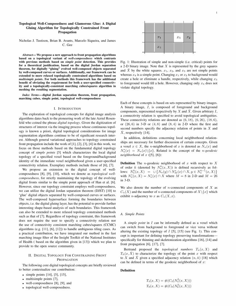
Fig. 1: Illustration of simple and non-simple (i.e. critical) points fora 2-D binary image. Note that X is represented by the grey squaresand X by the white squares. x1, x2, and x3 are not simple pointswhereas x4 is a simple point. Changing x1 or x2 to background wouldcreate a hole or eliminate a handle, respectively, while changing x3

to foreground would fill a hole. However, changing only x4 does notviolate digital topology.

Each of these concepts is based on sets represented by binary images.A binary image, I , is composed of foreground and backgroundcomponents, represented respectively by X and X . Given arbitrary I ,a connectivity relation is specified to avoid topological ambiguities.These connectivity relations are denoted as (6, 18), (6, 26), (18, 6),or (26, 6) in 3-D or (4, 8) and (8, 4) in 2-D where the first andsecond numbers specify the adjacency relation of points in X andX , respectively [14].

In addition, definitions concerning local neighborhood relation-ships are necessary for further discussion of certain concepts. Givena voxel x ∈ X , the n-neighborhood of x is denoted as Nn(x) andN∗

n(x) = Nn(x)\{x}. Related is the concept of the n-geodesicneighborhood of x ([5], [6]):

Definition The n-geodesic neighborhood of x with respect to Xof order k (denoted by Nk

n(x,X)) is defined recursively as fol-lows: Nk

n(x,X) = ∪{Nn(y) ∩N∗

M (x) ∩X, y ∈ Nk−1n (x,X)

}with N1

n(x,X) = N∗n(x) ∩X where M = 8 in 2-D and M = 26

in 3-D.

We also denote the number of n-connected components of X asCn(X) and the number of n-connected components of X\{x} whichexhibit n-adjacency to x as Cn(X,x).

A. Simple Points

A simple point in I can be informally defined as a voxel whichcan switch from background to foreground or vice versa withoutaltering the existing topology of I [5], [15] (see Fig. 1). This con-cept is important for defining topology preserving transformations—specifically for thinning and skeletonization algorithms [16], [14] andfront propagation [6], [17], [7].

Bertrand proposed the topological numbers Tn(x,X) andTn(x, X) to characterize the topology of the point x with respectto X and X given a specified adjacency relation (n, n) [18] whichcan be defined in terms of the geodesic neighborhood of x:

Definition

T4(x,X) = #(C4(N24 (x,X)))

T8(x,X) = #(C8(N28 (x,X)))

2

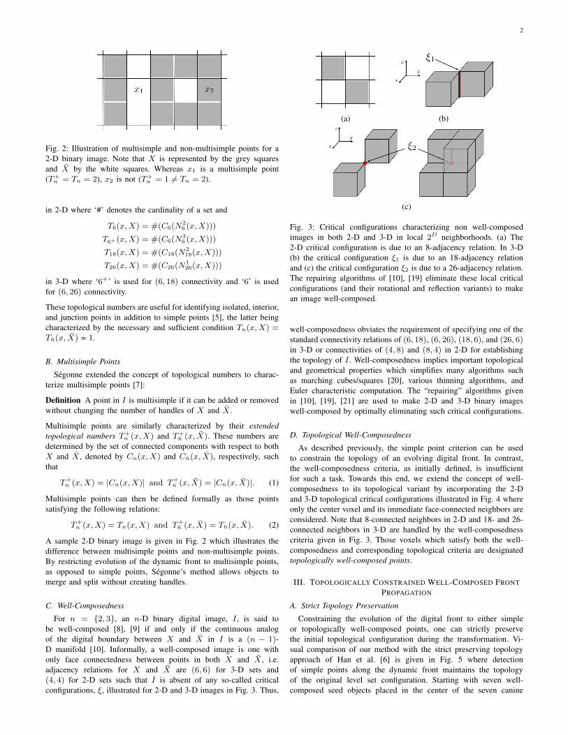
Fig. 2: Illustration of multisimple and non-multisimple points for a2-D binary image. Note that X is represented by the grey squaresand X by the white squares. Whereas x1 is a multisimple point(T+

n = Tn = 2), x2 is not (T+n = 1 6= Tn = 2).

in 2-D where ‘#’ denotes the cardinality of a set and

T6(x,X) = #(C6(N26 (x,X)))

T6+(x,X) = #(C6(N36 (x,X)))

T18(x,X) = #(C18(N218(x,X)))

T26(x,X) = #(C26(N126(x,X)))

in 3-D where ‘6+’ is used for (6, 18) connectivity and ‘6’ is usedfor (6, 26) connectivity.

These topological numbers are useful for identifying isolated, interior,and junction points in addition to simple points [5], the latter beingcharacterized by the necessary and sufficient condition Tn(x,X) =Tn(x, X) = 1.

B. Multisimple Points

Segonne extended the concept of topological numbers to charac-terize multisimple points [7]:

Definition A point in I is multisimple if it can be added or removedwithout changing the number of handles of X and X .

Multisimple points are similarly characterized by their extendedtopological numbers T+

n (x,X) and T+n (x, X). These numbers are

determined by the set of connected components with respect to bothX and X , denoted by Cn(x,X) and Cn(x, X), respectively, suchthat

T+n (x,X) = |Cn(x,X)| and T+

n (x, X) = |Cn(x, X)|. (1)

Multisimple points can then be defined formally as those pointssatisfying the following relations:

T+n (x,X) = Tn(x,X) and T+

n (x, X) = Tn(x, X). (2)

A sample 2-D binary image is given in Fig. 2 which illustrates thedifference between multisimple points and non-multisimple points.By restricting evolution of the dynamic front to multisimple points,as opposed to simple points, Segonne’s method allows objects tomerge and split without creating handles.

C. Well-Composedness

For n = {2, 3}, an n-D binary digital image, I , is said tobe well-composed [8], [9] if and only if the continuous analogof the digital boundary between X and X in I is a (n − 1)-D manifold [10]. Informally, a well-composed image is one withonly face connectedness between points in both X and X , i.e.adjacency relations for X and X are (6, 6) for 3-D sets and(4, 4) for 2-D sets such that I is absent of any so-called criticalconfigurations, ξ, illustrated for 2-D and 3-D images in Fig. 3. Thus,

(a) (b)

(c)

Fig. 3: Critical configurations characterizing non well-composedimages in both 2-D and 3-D in local 2D neighborhoods. (a) The2-D critical configuration is due to an 8-adjacency relation. In 3-D(b) the critical configuration ξ1 is due to an 18-adjacency relationand (c) the critical configuration ξ2 is due to a 26-adjacency relation.The repairing algorithms of [10], [19] eliminate these local criticalconfigurations (and their rotational and reflection variants) to makean image well-composed.

well-composedness obviates the requirement of specifying one of thestandard connectivity relations of (6, 18), (6, 26), (18, 6), and (26, 6)in 3-D or connectivities of (4, 8) and (8, 4) in 2-D for establishingthe topology of I . Well-composedness implies important topologicaland geometrical properties which simplifies many algorithms suchas marching cubes/squares [20], various thinning algorithms, andEuler characteristic computation. The “repairing” algorithms givenin [10], [19], [21] are used to make 2-D and 3-D binary imageswell-composed by optimally eliminating such critical configurations.

D. Topological Well-Composedness

As described previously, the simple point criterion can be usedto constrain the topology of an evolving digital front. In contrast,the well-composedness criteria, as initially defined, is insufficientfor such a task. Towards this end, we extend the concept of well-composedness to its topological variant by incorporating the 2-Dand 3-D topological critical configurations illustrated in Fig. 4 whereonly the center voxel and its immediate face-connected neighbors areconsidered. Note that 8-connected neighbors in 2-D and 18- and 26-connected neighbors in 3-D are handled by the well-composednesscriteria given in Fig. 3. Those voxels which satisfy both the well-composedness and corresponding topological criteria are designatedtopologically well-composed points.

III. TOPOLOGICALLY CONSTRAINED WELL-COMPOSED FRONT

PROPAGATION

A. Strict Topology Preservation

Constraining the evolution of the digital front to either simpleor topologically well-composed points, one can strictly preservethe initial topological configuration during the transformation. Vi-sual comparison of our method with the strict preserving topologyapproach of Han et al. [6] is given in Fig. 5 where detectionof simple points along the dynamic front maintains the topologyof the original level set configuration. Starting with seven well-composed seed objects placed in the center of the seven canine

3

(a) (b)

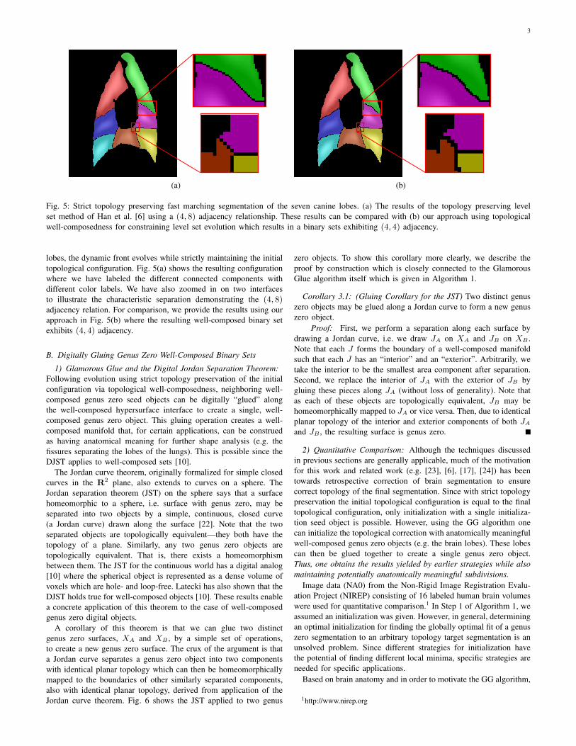
Fig. 5: Strict topology preserving fast marching segmentation of the seven canine lobes. (a) The results of the topology preserving levelset method of Han et al. [6] using a (4, 8) adjacency relationship. These results can be compared with (b) our approach using topologicalwell-composedness for constraining level set evolution which results in a binary sets exhibiting (4, 4) adjacency.

lobes, the dynamic front evolves while strictly maintaining the initialtopological configuration. Fig. 5(a) shows the resulting configurationwhere we have labeled the different connected components withdifferent color labels. We have also zoomed in on two interfacesto illustrate the characteristic separation demonstrating the (4, 8)adjacency relation. For comparison, we provide the results using ourapproach in Fig. 5(b) where the resulting well-composed binary setexhibits (4, 4) adjacency.

B. Digitally Gluing Genus Zero Well-Composed Binary Sets

1) Glamorous Glue and the Digital Jordan Separation Theorem:Following evolution using strict topology preservation of the initialconfiguration via topological well-composedness, neighboring well-composed genus zero seed objects can be digitally “glued” alongthe well-composed hypersurface interface to create a single, well-composed genus zero object. This gluing operation creates a well-composed manifold that, for certain applications, can be construedas having anatomical meaning for further shape analysis (e.g. thefissures separating the lobes of the lungs). This is possible since theDJST applies to well-composed sets [10].

The Jordan curve theorem, originally formalized for simple closedcurves in the R2 plane, also extends to curves on a sphere. TheJordan separation theorem (JST) on the sphere says that a surfacehomeomorphic to a sphere, i.e. surface with genus zero, may beseparated into two objects by a simple, continuous, closed curve(a Jordan curve) drawn along the surface [22]. Note that the twoseparated objects are topologically equivalent—they both have thetopology of a plane. Similarly, any two genus zero objects aretopologically equivalent. That is, there exists a homeomorphismbetween them. The JST for the continuous world has a digital analog[10] where the spherical object is represented as a dense volume ofvoxels which are hole- and loop-free. Latecki has also shown that theDJST holds true for well-composed objects [10]. These results enablea concrete application of this theorem to the case of well-composedgenus zero digital objects.

A corollary of this theorem is that we can glue two distinctgenus zero surfaces, XA and XB , by a simple set of operations,to create a new genus zero surface. The crux of the argument is thata Jordan curve separates a genus zero object into two componentswith identical planar topology which can then be homeomorphicallymapped to the boundaries of other similarly separated components,also with identical planar topology, derived from application of theJordan curve theorem. Fig. 6 shows the JST applied to two genus

zero objects. To show this corollary more clearly, we describe theproof by construction which is closely connected to the GlamorousGlue algorithm itself which is given in Algorithm 1.

Corollary 3.1: (Gluing Corollary for the JST) Two distinct genuszero objects may be glued along a Jordan curve to form a new genuszero object.

Proof: First, we perform a separation along each surface bydrawing a Jordan curve, i.e. we draw JA on XA and JB on XB .Note that each J forms the boundary of a well-composed manifoldsuch that each J has an “interior” and an “exterior”. Arbitrarily, wetake the interior to be the smallest area component after separation.Second, we replace the interior of JA with the exterior of JB bygluing these pieces along JA (without loss of generality). Note thatas each of these objects are topologically equivalent, JB may behomeomorphically mapped to JA or vice versa. Then, due to identicalplanar topology of the interior and exterior components of both JAand JB , the resulting surface is genus zero.

2) Quantitative Comparison: Although the techniques discussedin previous sections are generally applicable, much of the motivationfor this work and related work (e.g. [23], [6], [17], [24]) has beentowards retrospective correction of brain segmentation to ensurecorrect topology of the final segmentation. Since with strict topologypreservation the initial topological configuration is equal to the finaltopological configuration, only initialization with a single initializa-tion seed object is possible. However, using the GG algorithm onecan initialize the topological correction with anatomically meaningfulwell-composed genus zero objects (e.g. the brain lobes). These lobescan then be glued together to create a single genus zero object.Thus, one obtains the results yielded by earlier strategies while alsomaintaining potentially anatomically meaningful subdivisions.

Image data (NA0) from the Non-Rigid Image Registration Evalu-ation Project (NIREP) consisting of 16 labeled human brain volumeswere used for quantitative comparison.1 In Step 1 of Algorithm 1, weassumed an initialization was given. However, in general, determiningan optimal initialization for finding the globally optimal fit of a genuszero segmentation to an arbitrary topology target segmentation is anunsolved problem. Since different strategies for initialization havethe potential of finding different local minima, specific strategies areneeded for specific applications.

Based on brain anatomy and in order to motivate the GG algorithm,

1http://www.nirep.org

4

(a) (b)

(c)

(d) (e)

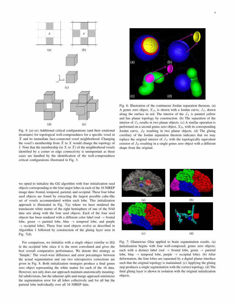
Fig. 4: (a)–(e) Additional critical configurations (and their rotationalinvariants) for topological well-composedness for a specific voxel inX and its immediate face-connected voxel neighborhood. Changingthe voxel’s membership from X to X would change the topology ofI . Note that the membership (in X or X) of the neighborhood voxelsidentified by a corner or edge connectivity is unimportant as thesecases are handled by the identification of the well-composednesscritical configurations illustrated in Fig. 3.

we opted to initialize the GG algorithm with four initialization seedobjects corresponding to the four major lobes in each of the 16 NIREPimage data: frontal, temporal, parietal, and occipital. These four lobarseed objects are found by extracting the largest possible cube-likeset of voxels accommodated within each lobe. This initializationapproach is illustrated in Fig. 7(a) where we have rendered thetranslucent white matter of the right hemisphere of one of the NA0data sets along with the four seed objects. Each of the four seedobjects has been rendered with a different color label (red → frontallobe, green → parietal lobe, blue → temporal lobe, and purple→ occipital lobe). These four seed objects evolve as described inAlgorithm 1 followed by construction of the gluing layer seen inFig. 7(d).

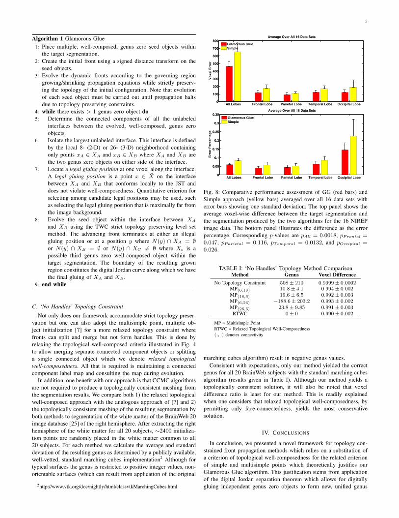
For comparison, we initialize with a single object (similar to [6])in the occipital lobe since it is the most convoluted and gives thebest overall comparative performance. We denote this strategy as‘Simple.’ The voxel-wise difference and error percentages betweenthe actual segmentation and our two retrospective corrections aregiven in Fig. 8. Both initialization strategies produce a final genuszero object representing the white matter for each of the 16 data.However, not only does our approach maintain anatomically meaning-ful subdivisions, but the inherent split-and-merge approach minimizesthe segmentation error for all lobes collectively and for all but theparietal lobe individually over all 16 NIREP data.

(a) (b)

(d)(c)

Fig. 6: Illustration of the continuous Jordan separation theorem. (a)A genus zero object, XA, is shown with a Jordan curve, JA, drawnalong the surface in red. The interior of the JA is painted yellowand has planar topology by construction. (b) The separation of theinterior of JA results in two planar objects. (c) A similar operation isperformed on a second genus zero object, XB , with its correspondingJordan curve, JB resulting in two planar objects. (d) The gluingcorollary of the Jordan separation theorem indicates that we mayreplace the original interior of JA with the topologically equivalentexterior of JB resulting in a single genus zero object with a differentshape from the original.

(a) (b)

(c) (d)

Fig. 7: Glamorous Glue applied to brain segmentation results. (a)Initialization begins with four well-composed, genus zero objects,each with a distinct label (red → frontal lobe, green → parietallobe, blue → temporal lobe, purple → occipital lobe). (b) Afterdeformation, the four lobes are separated by a digital planar interfacesuch that the original topology is maintained. (c) Applying the gluingstep produces a single segmentation with the correct topology. (d) Thefinal gluing layer is shown in isolation with the original initializationobjects.

5

Algorithm 1 Glamorous Glue1: Place multiple, well-composed, genus zero seed objects within

the target segmentation.2: Create the initial front using a signed distance transform on the

seed objects.3: Evolve the dynamic fronts according to the governing region

growing/shrinking propagation equations while strictly preserv-ing the topology of the initial configuration. Note that evolutionof each seed object must be carried out until propagation haltsdue to topology preserving constraints.

4: while there exists > 1 genus zero object do5: Determine the connected components of all the unlabeled

interfaces between the evolved, well-composed, genus zeroobjects.

6: Isolate the largest unlabeled interface. This interface is definedby the local 8- (2-D) or 26- (3-D) neighborhood containingonly points xA ∈ XA and xB ∈ XB where XA and XB arethe two genus zero objects on either side of the interface.

7: Locate a legal gluing position at one voxel along the interface.A legal gluing position is a point x ∈ X on the interfacebetween XA and XB that conforms locally to the JST anddoes not violate well-composedness. Quantitative criterion forselecting among candidate legal positions may be used, suchas selecting the legal gluing position that is maximally far fromthe image background.

8: Evolve the seed object within the interface between XA

and XB using the TWC strict topology preserving level setmethod. The advancing front terminates at either an illegalgluing position or at a position y where N(y) ∩ XA = ∅or N(y) ∩ XB = ∅ or N(y) ∩ XC 6= ∅ where Xc is apossible third genus zero well-composed object within thetarget segmentation. The boundary of the resulting grownregion constitutes the digital Jordan curve along which we havethe final gluing of XA and XB .

9: end while

C. ‘No Handles’ Topology Constraint

Not only does our framework accommodate strict topology preser-vation but one can also adopt the multisimple point, multiple ob-ject initialization [7] for a more relaxed topology constraint wherefronts can split and merge but not form handles. This is done byrelaxing the topological well-composed criteria illustrated in Fig. 4to allow merging separate connected component objects or splittinga single connected object which we denote relaxed topologicalwell-composedness. All that is required is maintaining a connectedcomponent label map and consulting the map during evolution.

In addition, one benefit with our approach is that CCMC algorithmsare not required to produce a topologically consistent meshing fromthe segmentation results. We compare both 1) the relaxed topologicalwell-composed approach with the analogous approach of [7] and 2)the topologically consistent meshing of the resulting segmentation byboth methods to segmentation of the white matter of the BrainWeb 20image database [25] of the right hemisphere. After extracting the righthemisphere of the white matter for all 20 subjects, ∼2400 initializa-tion points are randomly placed in the white matter common to all20 subjects. For each method we calculate the average and standarddeviation of the resulting genus as determined by a publicly available,well-vetted, standard marching cubes implementation2 Although fortypical surfaces the genus is restricted to positive integer values, non-orientable surfaces (which can result from application of the original

2http://www.vtk.org/doc/nightly/html/classvtkMarchingCubes.html

All Lobes Frontal Lobe Parietal Lobe Temporal Lobe Occipital Lobe0

100

200

300

400

500

600

700

800

Vox

el E

rror

Average Over All 16 Data Sets

Glamorous GlueSimple

All Lobes Frontal Lobe Parietal Lobe Temporal Lobe Occipital Lobe0

0.05

0.1

0.15

0.2

0.25

0.3

0.35

Err

or P

erce

ntag

e

Average Over All 16 Data Sets

Glamorous GlueSimple

Fig. 8: Comparative performance assessment of GG (red bars) andSimple approach (yellow bars) averaged over all 16 data sets witherror bars showing one standard deviation. The top panel shows theaverage voxel-wise difference between the target segmentation andthe segmentation produced by the two algorithms for the 16 NIREPimage data. The bottom panel illustrates the difference as the errorpercentage. Corresponding p-values are pAll = 0.0018, pFrontal =0.047, pParietal = 0.116, pTemporal = 0.0132, and pOccipital =0.026.

TABLE I: ‘No Handles’ Topology Method ComparisonMethod Genus Voxel Difference

No Topology Constraint 508± 210 0.9999± 0.0002MP(6,18) 10.8± 4.1 0.994± 0.002MP(18,6) 19.6± 6.5 0.992± 0.003MP(6,26) −188.6± 203.2 0.993± 0.002MP(26,6) 23.8± 9.85 0.991± 0.003

RTWC 0± 0 0.990± 0.002

MP = Multisimple PointRTWC = Relaxed Topological Well-Composedness(·, ·) denotes connectivity

marching cubes algorithm) result in negative genus values.Consistent with expectations, only our method yielded the correct

genus for all 20 BrainWeb subjects with the standard marching cubesalgorithm (results given in Table I). Although our method yields atopologically consistent solution, it will also be noted that voxeldifference ratio is least for our method. This is readily explainedwhen one considers that relaxed topological well-composedness, bypermitting only face-connectedness, yields the most conservativesolution.

IV. CONCLUSIONS

In conclusion, we presented a novel framework for topology con-strained front propagation methods which relies on a substitution ofa criterion of topological well-composedness for the related criterionof simple and multisimple points which theoretically justifies ourGlamorous Glue algorithm. This justification stems from applicationof the digital Jordan separation theorem which allows for digitallygluing independent genus zero objects to form new, unified genus

6

zero objects. An additional advantage is the elimination of CCMCalgorithmic requirements for meshing the resulting segmentation.

REFERENCES

[1] T. C. Cecil, “Numerical methods for partial differential equations in-volving discontinuities,” Ph.D. dissertation, University of California, LosAngeles, 2003.

[2] O. Alexandrov and F. Santosa, “A topology-preserving level set methodfor shape optimization,” Journal of Computational Physics, vol. 204,no. 1, pp. 121–130, 2005.

[3] G. Sundaramoorthi and A. Yezzi, “Global regularizing flows withtopology preservation for active contours and polygons.” IEEE TransImage Process, vol. 16, no. 3, pp. 803–812, Mar 2007.

[4] C. L. Guyader and L. A. Vese, “Self-repelling snakes for topology-preserving segmentation models.” IEEE Trans Image Process,vol. 17, no. 5, pp. 767–779, May 2008. [Online]. Available:http://dx.doi.org/10.1109/TIP.2008.919951

[5] G. Bertrand, “Simple points, topological numbers and geodesic neigh-borhoods in cubic grids,” Pattern Recognit. Lett., vol. 15, no. 10, pp.1003–1011, 1994.

[6] X. Han, C. Xu, and J. Prince, “A topology preserving level set methodfor geometric deformable models,” IEEE Trans. Pattern Analysis andMachine Intelligence, vol. 25, no. 6, pp. 755–768, 2003.

[7] F. Segonne, “Active contours under topology control–genus preservinglevel sets,” Int. J. Comput. Vision, vol. 79, no. 2, pp. 107–117, 2008.

[8] L. Latecki, U. Eckhardt, and A. Rosenfeld, “Well-composed sets,”Computer Vision and Image Understanding, vol. 61, pp. 70–83, 1995.

[9] L. J. Latecki, “3D well-composed pictures,” Graphical Models andImage Processing, vol. 59, no. 3, pp. 164–172, 1997.

[10] L. Latecki, Discrete Representation of Spatial Objects in ComputerVision. Springer, 1998.

[11] J.-O. Lachaud and A. Montanvert, “Continuous analogs of digitalboundaries: a topological approach to iso-surfaces,” Graphical models,vol. 62, no. 3, pp. 129–164, 2000.

[12] T. Lewiner, H. Lopes, A. W. Vieira, and G. Tavares, “Efficient implemen-tation of marching cubes’ cases with topological guarantees,” Journal ofgraphics, gpu, and game tools, vol. 8, no. 2, pp. 1–15, 2003.

[13] J. A. Sethian, Level Set Methods and Fast Marching Methods: EvolvingInterfaces in Computational Geometry, Fluid Mechanics, ComputerVision, and Materials Science. Cambridge University Press, 1999.

[14] T. Y. Kong and A. Rosenfeld, “Digital topology: Introduction andsurvey,” Computer Vision, Graphics, and Image Processing, vol. 48, pp.357–393, 1989.

[15] G. Bertrand, “A boolean characterization of three-dimensional simplepoints,” Pattern Recognit. Lett., vol. 17, pp. 115–124, 1996.

[16] A. Rosenfeld, “Connectivity in digital pictures,” J. ACM, vol. 17, pp.146–160, 1970.

[17] P.-L. Bazin and D. L. Pham, “Topology-preserving tissue classificationof magnetic resonance brain images.” IEEE Trans Med Imaging,vol. 26, no. 4, pp. 487–496, Apr 2007. [Online]. Available:http://dx.doi.org/10.1109/TMI.2007.893283

[18] G. Bertrand and G. Malandain, “A new characterization of three-dimensional simple points,” Pattern Recogn. Lett., vol. 15, no. 2, pp.169–175, 1994.

[19] M. Siqueira, L. J. Latecki, N. Tustison, J. Gallier, and J. Gee, “Topolog-ical repairing of 3-D digital images,” Journal of Mathematical Imagingand Vision, vol. 30, no. 3, pp. 249–274, March 2008.

[20] W. E. Lorenson and H. E. Cline, “Marching cubes: A high resolution3d surface construction algorithm,” Computer Graphics, vol. 21, no. 4,pp. 163–169, 1987.

[21] N. J. Tustison, M. Siqueira, and J. C. Gee, “Well-composedness andthe topological repairing of digital images,” The Insight Journal, 2007.[Online]. Available: http://hdl.handle.net/1926/470

[22] M. Nakahara, Geometry, Topology and Physics. Taylor and Francis,2003.

[23] D. W. Shattuck and R. M. Leahy, “Automated graph-based analysisand correction of cortical volume topology.” IEEE Trans Med Imaging,vol. 20, no. 11, pp. 1167–1177, Nov 2001. [Online]. Available:http://dx.doi.org/10.1109/42.963819

[24] P.-L. Bazin and D. L. Pham, “Homeomorphic brain imagesegmentation with topological and statistical atlases.” Med ImageAnal, vol. 12, no. 5, pp. 616–625, Oct 2008. [Online]. Available:http://dx.doi.org/10.1016/j.media.2008.06.008

[25] B. Aubert-Broche, M. Griffin, G. B. Pike, A. C. Evans, and D. L. Collins,“Twenty new digital brain phantoms for creation of validation image databases.” IEEE Trans Med Imaging, vol. 25, no. 11, pp. 1410–1416, Nov2006. [Online]. Available: http://dx.doi.org/10.1109/TMI.2006.883453