Topological numbers and singularities in scalar images: Scale-space evolution properties

P1: TPR/NKD P2: JSN/ASH/PCY QC: JSN

Journal of Mathematical Imaging and Vision KL645-04-Kalitzin September 28, 1998 19:54

Journal of Mathematical Imaging and Vision 9, 253–269 (1998)c© 1998 Kluwer Academic Publishers. Manufactured in The Netherlands.

Topological Numbers and Singularities in Scalar Images:Scale-Space Evolution Properties

STILIYAN N. KALITZIN, BART M. TER HAAR ROMENY, ALFONS H. SALDEN,PETER FM NACKEN, AND MAX A. VIERGEVER

Abstract. Singular points of scalar images in any dimensions are classified by a topological number. This numbertakes integer values and can efficiently be computed as a surface integral on any closed hypersurface surroundinga given point. A nonzero value of the topological number indicates that in the corresponding point the gradientfield vanishes, so the point is singular. The value of the topological number classifies the singularity and extendsthe notion of local minima and maxima in one-dimensional signals to the higher dimensional scalar images.Topological numbers are preserved along the drift of nondegenerate singular points induced by any smooth imagedeformation. When interactions such as annihilations, creations or scatter of singular points occurs upon a smoothimage deformation, the total topological number remains the same.

Our analysis based on an integral method and thus is a nonperturbative extension of the order-by-order approachusing sets of differential invariants for studying singular points.

Examples of typical singularities in one- and two-dimensional images are presented and their evolution inducedby isotropic linear diffusion of the image is studied.

Keywords: singular points, scalar images, topology, catastrophes, scale space

1. Introduction

Scale-space approaches [16] provide tools for studyinga given image at all scales simultaneously. Featuresthat can be detected at large scales can provide cluesfor tracing more detailed information at fine scales. Forthis ideology to be constructive, one needs to investi-gate whichlocal properties (or local operators) are ap-propriate for quantifying the desired features and howthese properties are changing from scale to scale. Invarious applications that involve the study of orientedimage structures [5], singular points are of particularinterest. Singular points, or singularities in the sequel,are those points in a grey-scale image, where the gra-dient vector field vanishes [4, 7]. Examples of suchpoints in two-dimensional images are extrema, sad-dle points, “monkey” saddles etc. Singularities can becharacterized by their order. The order of a singularpoint is the lowest nonvanishing power in the Taylorexpansion of the image fieldL(x1, x2, . . . , xd) aroundthis point. Obviously, the order must be greater than 1,

since the gradient vectorLi = ∂i L(x1, x2, . . . , xd) isequal to zero in this point.

We propose in this paper an additional topologicalcharacteristic, or number, which can classify singu-larity points of an image. Its definition is completelynonperturbative in the sense that it makes no referenceto any higher order differential structures (forming thecoefficients in any Taylor expansion) around the singu-larity [4, 7, 12, 14]. Instead, this number is computedas an integral on a hypersurface closely surrounding thesingular point. Nonperturbative integral quantities hasbeen introduced in [15], but they are of a nontopologicalnature. The topological features of the quantity con-sidered in this article are revealed by its large class ofinvariances. The topological number associated to anisolated singular point is independent, for example, onthe choice of the hypersurface which it is computed on.

For a surface-integral, nonperturbative definition tobe well-posed, we must ensure that our image fieldcontains only isolated singularities. If the image is con-volved with a Gaussian kernel, then all derivatives are



254 Kalitzin et al.

well defined [3] and it is well known that the image fieldwill have only isolated singularities [9]. The amountof blurring, or the scale, will be treated according tothe scale-space paradigm as an independent “coordi-nate” t . The blurred image is a solution of the lineardiffusion equation [6]

∂t L(x, t) = 1L(x, t), (1)

with the scalar image as an initial condition. Here we as-sumed spatial dimensions so, unless otherwise stated,we use the abbreviationx = {x1, . . . , xd}. When thescale is considered fixed at some value and the depen-dence on it is not explicitly used, thet variable will beomitted in our formulas.

The topological number considered below is the nat-ural quantity that describes singularities in all imagedimensions. For one-dimensional signals this quan-tity reduces to a binary number indicating points oflocal maxima or minima. For two-dimensional signalsthis number (known also as the winding number for thegradient vector field) extends the definitions of extremaand saddle points that characterize the nondegeneratesingularities, for the degenerate, higher order cases.Winding numbers have been introduced for analyzingsingularities in two-dimensional oriented patterns [5].Here we give a more general approach including anyorder of singularity and any number of image dimen-sions.

By computing the topological number in every(scale) space point, we can define in a consistent waya (scale) spacedistribution , or density, of the topolo-gical “charge”. This density provides a practical toolfor localization of the singularity points and thus con-tains both spatial information and information aboutthetype of the singularities.

When scale space evolution is considered, singula-rity points “drift” and eventually interact with eachother in the so-called catastrophe points [4]. The topo-logical number has a conservation property which en-ables to analyze the outcome of these interactions.

This article is organized as follows. In the followingsection we give a self-contained theoretical descriptionof the topological numbers and their major properties.The scale parameter introduced by the scale-space dy-namics (1) is considered fixed and serves only as aregularizing parameter that makes differentiation wellposed.

Section 3 is devoted to some low-dimensional orlow-order applications of the general definitions. First,

we consider second-order singularities and show thatfor any number of image dimensions the topologicalnumber (13) is proportional to the sign of the Hessian.Next, we study general singularities for one- and two-dimensional images and for the last case we apply analternative method for computing the topological num-bers. The last uses the complex representation of scalarimages and relates the topological number of a singu-lar point to the number of roots on the unit disc of anappropriately image-derived analytic function.

Section 4 introduces the scale-space dynamics andconsiders the evolution of the singularities. Conser-vation and additive properties of the topological num-ber allow the introduction of a conserved current thatcharacterizes the flow of singularities in the scale space.This current obeys the Kirchoff conservation law at thetop-points (degenerate singularities where singularitiesinteract in scale space [4]). In this section we give alsoa briefperturbative analysis of the top points.

Examples of the typical one- and two-dimensionaltop points are considered in Section 5 as an illustra-tion of the topological number conservation propertypresented in Section 4.

In Section 6, we use the local density of topologicalnumbers to propose a weak causality principle for anydiffusion scheme.

Finally, in Section 7 we summarize the propertiesof the topological number considered in this paperand discuss possible applications to image processing.Some open questions and suggestions for further re-search are considered.

2. Topological Invariants in Scalar Images

Now we introduce some brief notations from the the-ory of homotopy groups [11]. They provide the natu-ral basis for the introduction of a topological numberassociated to any singular image point. To understandthe rest of the paper, however, no explicit knowledgeof this theory is required. In the following, we giveself-contained definitions of our quantities as well as adetailed proof of their essential properties.

SupposeP is a point in the image (singular orregular) andVP is a region aroundP which doesnot contain any singularities except possiblyP. Nowwe will define a quantity characterizing the image inthe surrounding of the pointP. Let SP be a closedhypersurface, topologically equivalent to a(d − 1)-dimensional sphere, such that it is entirely inVP andour test pointP is inside the regionWP bounded bySP.



Topological Numbers and Singularities 255

In other words,

P ∈ WP : SP = ∂WP. (2)

Because by assumption there are no singularities inSP ∈ VP, the normalized gradient vector field

ξi = ∂i L

(∂ j L∂ j L)1/2(3)

Li ≡ ∂i L (4)

is well defined on the surfaceSP. Throughout this pa-per, a sum over all repeated indices is assumed.

The space of all unit-lengthd-dimensionalEuclidean vectors is isomorphic to the(d − 1)-dimensional sphere of unit radiusS(d−1)

1 . Therefore,the vector fieldξi defines a mapping

SP → S(d−1)1 .

But recalling that(SP) is a manifold homotopic to a(d − 1)-dimensional sphere, we see that the abovemapping can be classified by an element of the ho-motopy groupπ(d−1)(S(d−1)). This group comprisesall homotopically nonequivalent mappings betweentwo (d − 1)-dimensional spheres. It is known thatπ(d−1)(S

(d−1)1 ) ≡ Z which is the Abelian group of all

integer numbers (where addition is the group opera-tion). Without plunging further into the theory of ho-motopy groups, we can characterize the vector fieldξi

on the surfaceSP taken around the chosen pointP bythe homotopy number (the element ofπ(d−1)(S(d−1)))

of the mapping it defines. This numberν is indepen-dent of the surfaceSP as long asSP ∈ VP, since thenthe surface does not surround singularities other thanpossiblyP. Therefore, the so defined local topologicalnumberν characterizes only the image neighborhoodof the pointP and not the hypersurface on which it ismeasured.

To make the above statements and ideas explicit,we first give the operational definition of the quantityν (without any reference to the theory of homotopygroups).

Definition 1. Let L(x) : Rd → R be a differentiabled-dimensional scalar image represented by itsgrey-scale functionwith at most isolated singularity points.At a nonsingular point A = (x1, . . . , xd) we define a

d − 1 form:

8(A)= ξi1dξi2 ∧ · · · ∧ dξidεi1i2,...,i d (5)

ε i1i2,...,i k...,i l ,...,id =−ε i1i2,...,i l ,...,i k,...,id for anyl 6= k;ε12,...,d= 1. (6)

Definition 2. In the same conditions as in Definition 1,and furthermore letS, be a closed(∂S= 0), orientedhypersurface. If there are no singularities onSthen wedefine the quantity:

νS =∮

A∈S8(A). (7)

The above integral is the natural integral of a(d− 1)form over a(d−1)-dimensional manifold without bor-der.

The following proposition gives an equivalent ex-pression for8 (and therefore forνS):

Proposition 1.

8(A) = Li1dLi2 ∧ · · · ∧ dLidεi1i2,...,id

(L j (A)L j (A))d/2(8)

Proof: From the definition (4) forξi follows

dξi = dLi

(L j L j )1/2− Li

LkdLk

(L j L j )3/2. (9)

Replacing this expression in (8), we see from the pres-ence of anLi factor and from the antisymmetry of theε tensor that the second term will not contribute.2

An important property of thed− 1 form8 is that itis a closed form, or:

Proposition 2.

d8(A) = 0. (10)

Proof: From the definition of8 in (5) and the basicproperty of the exterior derivatived ∧ d ≡ 0 we have

d8(A) = dξi1 ∧ dξi2 ∧ · · · ∧ dξidεi1i2,...,id

≡ d!dξ1 ∧ · · · ∧ dξd. (11)

Recalling thatξ is a vector with a unit length, we notethat ξi dξi ≡ ξ1dξ1 + · · · + ξddξd = 0 whereverξis defined. This linear constraint together with (11)gives (10). 2



256 Kalitzin et al.

The above property of the form (5) is essential forthe applications of the topological quantity (7). IfWis a region where the image has no singularities, thenthe form8 is defined for the entire regionW and wecan apply the generalized Stoke’s theorem [1, 2]:∮

∂W8(d−1) =

∫W

d8(d−1) ≡ 0 (12)

because of (10). Therefore, we obtain the followingcorollary:

Corollary 1. If the grey-scale function has no singu-larities in a given region W, then the topological quan-tity (7) computed on its border is identically zero.

Consider now a smooth local deformation of the sur-faceS. If no singularities are crossed byS in the pro-cess of this deformation, then the region swept by thesurface will be free of singularities and therefore thetopological number on its border is zero. But the bor-der of this region is composed exactly of the initialsurface, with its orientation inverted, and the deformedsurface. It is easy to see that the number (7) is additiveor, in other wordsνS1∪S2 = νS1 + νS2 whereS1 andS2

are two hypersurfaces. The integral definingνS obvi-ously changes its sign when changing the orientation ofthe surface of integration. Therefore, the quantity (7)on the initial and the deformed surfaces are equal astheir difference is zero. This leads to the following:

Corollary 2. The topological number(7) is invariantunder smooth deformations of the hyper surface S, aslong as in the process no singularities are crossed.

The last property justifies the term “topological” thatwe assign to the quantityνS. It depends on the proper-ties of the image in the region whereS is placed, but, ingeneral, not on the surfaceS itself. More precisely, aswe shall see later, the topological number depends onlyon the number and type of singularities surrounded bythe surfaceS.

So far we considered a topological numberνS associ-ated with a given hypersurface. Suppose now that, as inthe beginning of this section, we have a selected pointP in the image and letSP be a hypersurface aroundPsuch that in the regionWP bounded bySP(∂WP = SP),there are no singularities except possiblyP. Then it isclear from the Corollary 2 that the numberν computedfor this surface will be invariant under any deforma-tions of S as long as no singular points are crossed.

Therefore, for any image pointP we can define thetopological number as:

Definition 3.

νP =∮

A∈S8(A) (13)

where S is any closed oriented hypersurface takenclosely aroundP. The surfaceS must be close toPin order to ensure that no other singularities are sur-rounded.

In this paper we deal only with topological numbersassociated with the close neighborhoods of the points inthe image. In this sense this topological description isan extension of the analysis of the local differential in-variants and should be considered as a complementarytechnique [13]. Given a scalar image, we can computethe quantity (13) for each point and analyze the dis-tribution of the different types of singular points. Anadvantage of the above approach is that the topologicalnumber takes discrete sets of values (see the beginningof this section) and therefore it is easy and natural to bethresholded. For example, we can select only singu-larities with topological number+1,−1 or any otherinteger value. Another convenient property, as we sawin deriving Corollary 2, is that (7) computed around agiven region is additive when the region is split intoseveral subregions. Therefore, two singularities closeto each other will have a combined topological numberequal to the sum of their individual ones. This propertywill be essential when we study the scale evolution ofthe singularities.

An important property of the topological num-bers (7) and (13) is that they are grey-scale invari-ants. Consider a transformation of the formL(x, t)→3(L(x, t)), where3 is a real, strictly monotonic func-tion, or in other words∂3

∂L > 0 everywhere. Then forthe new image3(x, t), quantities (13) and (7) remainthe same.

Proposition 3. Topological numbers(13) and(7) as-sociated respectively with every point or with every hy-persurface of the image are invariant under strictlymonotonic functional transformations of the imagefield.

Proof: From the definition (4), the normalized gra-dient field computed for the transformed image will be




equal to the original one. Indeed,

∂i3

(∂ j3∂ j3)1/2= ∂i L

(∂ j L∂ j L)1/2∂3/∂L

|∂3/∂L| . (14)

But the last factor is 1 in every point onS because3is strictly monotonic. 2

The last proposition can be generalized to the fol-lowing “conservation law”:

Proposition 4. Let νS be defined as in Definitions1and 2 and let L(x, λ), λ ∈ [0, 1] be a oneparameterfamily of images, smoothly depending on the deforma-tion parameterλ, such that L(x, 0) = L(x). If the newfield L(x, λ) has no singularities on the hypersurfaceS for any value ofλ ∈ [0, 1], then quantityνS(λ) givenin (5) and(7) for the field L(x, λ), is the same for allλ ∈ [0, 1].

Proof: The fieldL(x, λ)has no singularities onSandtherefore its gradient vector can be normalized for allλ ∈ [0, 1]. Taking both theλ-derivative and exteriorderivative of the normalization equationξi ξi ≡ 1, weobtain:

∂λξi ξi = 0,

dξi ξi = 0.(15)

From (15) we conclude that∂λξ is orthogonal toξand therefore, we have the decomposition

∂λξi =d−1∑

1

Bαηαi ,

dξi =d−1∑

1

Cαηαi , (16)

α = 1, . . . ,d − 1,

whereBα ared−1 scalar parameters,Cα ared−1 one-forms andηα ared − 1 linearly independent vectors,orthogonal toξ .

Theλ-derivative of the topological numberνS is

∂λνS =∮

S∂λ(ξi1dξi2, . . . ,dξidε

i1i2,...,id)

= (d)∮

S∂λξi1dξi2, . . . ,dξidε

i1i2,...,id (17)

To obtain the last equality, we have integrated by partsthe terms with∂λdξ ≡ d∂λξ and used the antisym-metry ofε. Finally, substituting∂λξ anddξi from (16),we find that an antisymmetric product ofd vectorsηα

appears as a common factor. But this is identically zerobecause there are onlyd−1 of these vectors. Therefore∂λνS ≡ 0. 2

The last proposition is of fundamental importancewhen smooth image evolution is considered. Such evo-lution can be induced, for example, by the diffusionequation (1) or by any other flow or deformation. Thetopological number of a given closed (always assumedoriented) hypersurface will not change unless singula-rities are crossing it during the evolution. Singularitiesmay merge, scatter, annihilate each other etc., but thesum of the topological numbers of a group of singularpoints in a given region will remain the same as longas no singularities are coming into the region and nosingularities are leaving this region. We will come tothis issue later when considering the evolution of thesingularities across the scale space.

Topological numbersνP can be associated with ev-ery point of the image. It is clear from Proposition 2and the integral Stoke’s theorem (12), however, thatthe topological number of a nonsingular point is zero.If we plot the value ofνP in every point of an image,we will obtain a map of the singularities of the im-age representing their topological “charge”. We cango one step further and define ascalar density field,ν(x1, x2, . . . , xd), that gives thedistribution of thetopological singularities in a given image.

Definition 4. Let νP be the number given by (13) foran arbitrarily selected pointP. Let SP be the hypersur-face in (13) aroundP andWP be the region boundedby SP. First, we define the followingRd → R functionas:

νP,SP (x) ={νP if x ∈ WP;0 otherwise.

. (18)

Now we can define thedistribution associated withthe topological numberin the point P as

νP(x) = limSp→0

1

|WSP |νP,SP (x) (19)

whereWSP is the Euclidean region ofWP and the limitis take for SP shrinking to a point. It is clear fromCorollary 2 that this limit is well defined.



258 Kalitzin et al.

When all points of the image are considered, the totaldistribution of the topological number is defined as:

ν(x) =∑P∈R2

νP(x). (20)

As the contributions from the regular points is identi-cally zero, the above sum is over only the discrete subsetof singularities in the image. This justifies the use of asum in (20), rather than of an integral over the imagespace.

Formula (20) can be computed exactly and gives:

Proposition 5. The distribution of the topologicalnumbers of an image with isolated singularities is

ν(x) =∑

P

νPδ(x − xP), (21)

whereνP are the topological numbers(13), δ(x) is thed-dimensional Dirac delta distribution, and the sumis over allsingular points in the image. The last areassumed to be in the discrete set of locations xP.

Proof: Let µ(x) be a test function,µ(x) ∈ C2(Rd).To prove (21) we consider the integral∫

R2µ(x)ν(x) =

∑P

∫R2µ(x)νP(x)

=∑

P

limSP→0

1

|WSP |∫

R2µ(x)νP,SP (x),

(22)

where the definitions (20) and (19) have been used.But in the last integral, because of Corollary 2 and thedefinition (18), we have∫

R2µ(x)νP,SP (x) = νP

∫WP

µ(x). (23)

As the hypersurfaceSP shrinks to a point, the last integ-ral givesµ(xP)WP (sinceµ(x) is a smooth function).So for any test functionµ(x) we have∫

R2µ(x)ν(x) =

∑P

νPµ(xP). (24)

This proves Eq. (21). 2

So with each image fieldL(x)we can associate a dis-tribution field of its singularitiesν(x) as defined above.

In practice though, when we give a graphical presen-tation of the singularities of an image, as for examplein Fig. 1, we can only deal with thespatial regular-izations of these distributions. Such a regularizationis the function

∑P νP,SP (x) obtained as a sum of the

individual functions from (18). In this last function, thetopological quantities are computed on a chosen set ofsurfaces, surrounding each singular point. The size (inany sense) of these surfaces will appear as an exter-nal measurement scale. In fact, this scale determinesto what precision we consider two closely positionedsingularities as separate.

3. Examples of Topological Numbers

In this section we present some particular cases, wherethe theory presented in the previous section can be illus-trated and the topological number can be computedanalytically.

3.1. Second-Order Singularities

Nondegenerate, or Morse, singularities are those pointswhere the gradient vector vanishes, but the determinantof the Hessian is nonzero. For these cases the topolo-gical number represents the sign of this determinant.

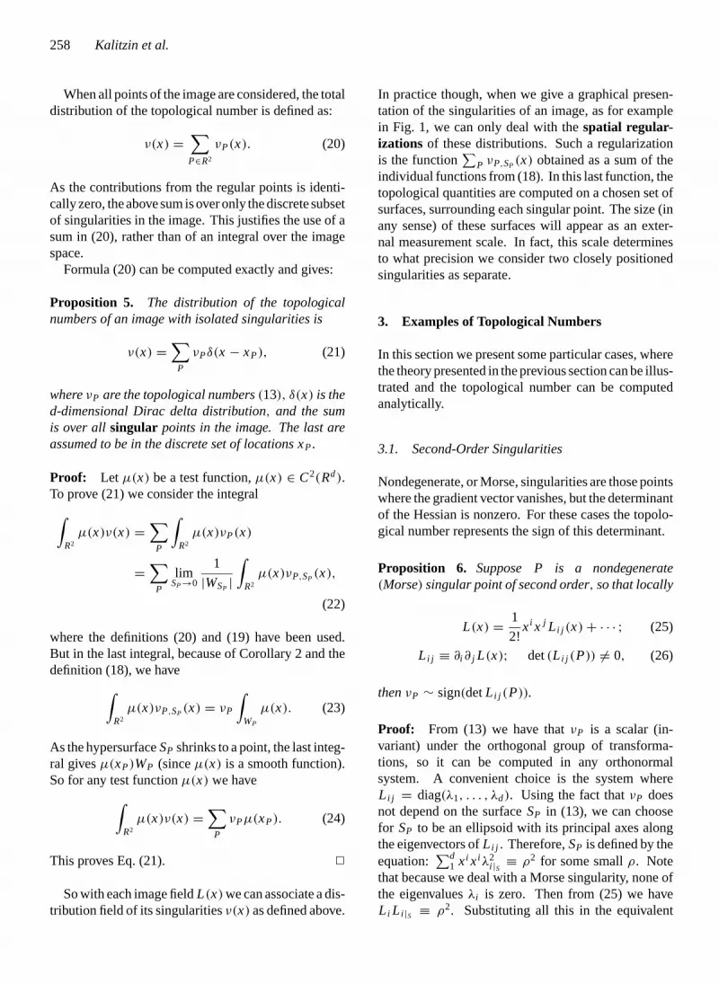
Proposition 6. Suppose P is a nondegenerate(Morse) singular point of second order, so that locally

L(x) = 1

2!xi x j Li j (x)+ · · · ; (25)

Li j ≡ ∂i ∂ j L(x); det(Li j (P)) 6= 0, (26)

thenνP ∼ sign(detLi j (P)).

Proof: From (13) we have thatνP is a scalar (in-variant) under the orthogonal group of transforma-tions, so it can be computed in any orthonormalsystem. A convenient choice is the system whereLi j = diag(λ1, . . . , λd). Using the fact thatνP doesnot depend on the surfaceSP in (13), we can choosefor SP to be an ellipsoid with its principal axes alongthe eigenvectors ofLi j . Therefore,SP is defined by theequation:

∑d1 xi xiλ2

i |S ≡ ρ2 for some smallρ. Notethat because we deal with a Morse singularity, none ofthe eigenvaluesλi is zero. Then from (25) we haveLi Li |S ≡ ρ2. Substituting all this in the equivalent




form (8) we have

νP = ρ−dd∏1

λi

∮S

xi1dxi2 ∧ · · · ∧ dxidεi1,...,id . (27)

Introducing new integration variables in (27)yi =xi |λi |ρ−1; yi yi ≡ 1, we get

νP =∏d

1 λi∏d1 |λi |

∮S1

yi1dyi2 ∧ · · · ∧ dyidεi1,...,id , (28)

whereS1 is the unitd−1 sphere and the integral is just aconstant depending only on the number of dimensions.The product ratio gives obviously the essential factorsign(detLi j ). 2

This proposition shows that the topological num-ber (7) can be considered also as an extension of thenotion of the sign of the determinant of the Hessian forthe cases where the last quantity vanishes.

Illustration for the nondegenerate singular pointtopological numbers is given in Fig. 1. There twoextrema (white dots) and two saddle points (blackdots) are localized by the winding number distribu-tion.

Now we switch to specific lower dimensional caseswhere the above definitions and propositions can becompared with more intuitive constructions.

3.2. One-Dimensional Case

For one-dimensional signalsL(x), the topologicalnumber (7) for a pointP= x is ultimately sim-ple: νP ≡ sign(Lx)B− sign(Lx)A for any A, B : A<P< B in the close vicinity ofP. In other words, thetopological number of a point is reduced to the differ-ence between the signs of the image derivative takenfrom the left and from the right. Obviously,νP = 2 forlocal minima,νP =−2 for local maxima andνP = 0for regular points or in-flex singularities.

Although this case is trivial, it shows that the gen-eral notion of topological quantity (7) reduces to thenatural concept of local minima and maxima in one-dimensional signals. For higher dimensional images,the topological number does not reduce to local extremaidentifier, but it provides a more subtle informationfor the behavior of the image around its singula-rities.

3.3. Two-Dimensional Images

For two-dimensional images the topological num-ber (13) labels the equivalent class of mappingsbetween two unit circles (see the beginning of theSection 2). This label is known also as the windingnumber. The winding number represents the numberof times that the normalized gradient turns around itsorigin, as a test point circles around a given contour(hypersurface ind = 2). Indeed, in two dimensionsthe one-form8 ≡ ξ × dξ in (5) gives just the anglebetween the normalized gradients in two neighboringpoints. Integrating this angle along a closed contour wefind the winding number associated with this contour.

Clearly, the winding number of any closed contourmust be an integer multiple of 2π . We can compute thisnumber directly from (13) and (5), but in two dimen-sions it is more convenient to use a complex-numberrepresentation.

Let z= x1+ i x2, z̄= x1− i x2 be the complex con-jugated couple of coordinates in the two-dimensionalimage space and letL(z, z̄) be the image in this nota-tion. Then the complex functionW = (L1+ i L 2)/2≡∂z̄L(z, z̄), whereLi ≡ ∂xi L, represents the gradientvector field in complex coordinates. Reality conditionimplies L(z, z̄) = L̄(z, z̄), ∂zW = ∂z̄W̄.

In accord with (5), we can present the form8(A) incomplex notation as:

8(A) = ξ1dξ2− ξ2dξ1 = (L1dL2− L2dL1)

(L1L1+ L2L2)

= Im(L1− i L 2)d(L1+ i L 2)

(L1L1+ L2L2)

= Im[W̄dW/(WW̄)] = Im(dW/W)

= Im(d ln(W)). (29)

The last equality clearly justifies the interpretation of8 as a relative angle change of the gradient field. Incomplex notations, this is just the phase (the imaginarypart of the complex logarithm) of the complex fieldW(z, z̄).

Using this equivalent representation, we can nowinvestigate the topological number for singularitiesgenerated by homogeneous polynomial structures ofa given order. If the image fieldL(x1, x2) is a ho-mogeneous polynomial of ordern, then by definitionL(λx1, λx2) ≡ λnL(x1, x2) for any numberλ and



260 Kalitzin et al.

therefore its complex representation is of the form:

L(z, z̄) =n∑

q=0

Cqzqz̄(n−q) (30)

with Cq = C̄n−q some complex coefficients. For thegradient fieldW we have:

W(z)|C =n−1∑q=0

(n− q)Cqzqz̄(n−q−1). (31)

Clearly, an image defined by the grey-scale func-tion (30) has a singular point at the originz = 0. Thewinding number generated by such a singularity canbe computed by investigating the complex roots of anappropriate analytic function. To this end, we need todefine an analytic functionF(η) of the complex argu-mentη ≡ z2.

Definition 5. Consider the gradient functionW(z, z̄)from (31) on the unit circleC1 : zz̄ ≡ 1. Then,W(z, z̄) ≡ W(z, z−1), or inserting this into (31):

W|C1 ≡ z−n+1n−1∑

0

(n− q)Cqz2q ≡ z−n+1U (z2) (32)

whereU (z2) is a polynomial defined onC1. Then wedefineF(η) as the unique analytic continuation in thecomplex planeη ≡ z2 of the functionU (η ≡ z2).Clearly, F(η) is a polynomial of maximal degree(n− 1).

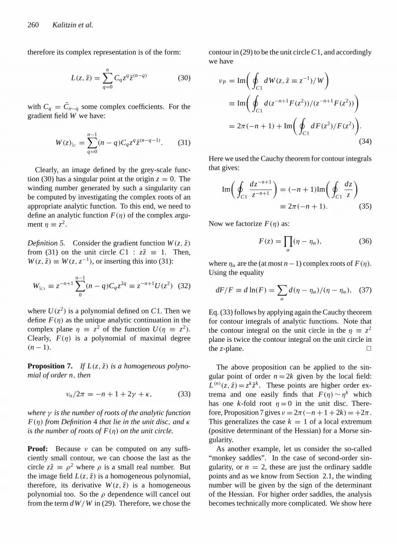
Proposition 7. If L (z, z̄) is a homogeneous polyno-mial of order n, then

νn/2π = −n+ 1+ 2γ + κ, (33)

whereγ is the number of roots of the analytic functionF(η) from Definition4 that lie in the unit disc, andκis the number of roots of F(η) on the unit circle.

Proof: Becauseν can be computed on any suffi-ciently small contour, we can choose the last as thecircle zz̄ ≡ ρ2 whereρ is a small real number. Butthe image fieldL(z, z̄) is a homogeneous polynomial,therefore, its derivativeW(z, z̄) is a homogeneouspolynomial too. So theρ dependence will cancel outfrom the termdW/W in (29). Therefore, we chose the

contour in (29) to be the unit circleC1, and accordinglywe have

νP = Im

(∮C1

dW(z, z̄≡ z−1)/W

)≡ Im

(∮C1

d(z−n+1F(z2))/(z−n+1F(z2))

)= 2π(−n+ 1)+ Im

(∮C1

d F(z2)/F(z2)

).

(34)

Here we used the Cauchy theorem for contour integralsthat gives:

Im

(∮C1

dz−n+1

z−n+1

)= (−n+ 1)Im

(∮C1

dz

z

)≡ 2π(−n+ 1). (35)

Now we factorizeF(η) as:

F(z) =∏α

(η − ηα), (36)

whereηα are the (at mostn−1) complex roots ofF(η).Using the equality

dF/F ≡ d ln(F) =∑α

d(η − ηα)/(η − ηα), (37)

Eq. (33) follows by applying again the Cauchy theoremfor contour integrals of analytic functions. Note thatthe contour integral on the unit circle in theη ≡ z2

plane is twice the contour integral on the unit circle inthez-plane. 2

The above proposition can be applied to the sin-gular point of ordern= 2k given by the local field:L(n)(z, z̄)= zkz̄k. These points are higher order ex-trema and one easily finds thatF(η)∼ ηk whichhas onek-fold root η= 0 in the unit disc. There-fore, Proposition 7 givesν= 2π(−n+ 1+ 2k)=+2π .This generalizes the casek = 1 of a local extremum(positive determinant of the Hessian) for a Morse sin-gularity.

As another example, let us consider the so-called“monkey saddles”. In the case of second-order sin-gularity, orn = 2, these are just the ordinary saddlepoints and as we know from Section 2.1, the windingnumber will be given by the sign of the determinantof the Hessian. For higher order saddles, the analysisbecomes technically more complicated. We show here




that in case of a nondegeneratenth order symmetricsaddle point, the winding number of the gradient fieldis 2π(−n+ 1).

A nondegeneratenth order symmetric saddle point(for simpler notations assumed atx1 = x2 = 0) isdefined locally by a grey-scale function of the form:

L(n)(z, z̄) = zn + z̄n, (38)

From Definition 5 we can directly find the analyticfunction F(η) ∼ 1. As a constant function, it has noroots at all, so Proposition 7 givesν = 2π(−n+ 1).

This image has a rosette type of structure aroundthe singular point and can be detected as a high-valuepoint of an appropriate (set of) differential invariant. Inour approach, such a point is just a point with negativewinding number,ν = 2π(−n+ 1) for somen.

It is clear that for two-dimensional images, the wind-ing number generalizes the notion of extrema and sad-dle points. The last are characterizing nondegeneratesingularities, where the Hessian can have positive ornegative determinant. When the singular point is de-generate, the determinant of the Hessian is zero and itdoes not quantify the singular point. The winding num-ber ν, on the other hand, represents information con-tained in the higher order jets in the degenerate singularpoint. More examples of singularities of a particularorder and their evolution in scale space is presented inthe next section.

4. Scale-Space Evolution

In the previous sections we considered the image fieldfor a fixed value of the scale parametert . The fact thatL(x, t) is a solution of the linear diffusion equation (1)was used only to ensure that the functionL(x, t) has atmost isolated singularities and that it is infinitely differ-entiable. Here we will reintroduce the explicit depen-dence of the grey-scale function on the scale parameter.In this sense, the image becomes a(d+ n)-dimensionalgrey-scale field. Singular points of each scale now willgroup in lines in the scale space, the so-called singular-ity strings. These singularity strings may occasionallyinteract with each other: scatter, annihilate etc. Fromthe point of view of the ordinary image space, the sin-gular strings are formed by the drifting of the singu-larities as a result of the deformation of the image.Then the events of interactions between the singulari-ties appear as a catastrophes (in Thom’s sense) [8, 10],where the scalet should be considered as a deformation

parameter. Such catastrophes are not linked intrinsi-cally to the diffusion equation, but as we discussed inthe Section 2, will occur within any scheme where theimage is smoothly deformed. For the rest of this sec-tion though, we deal only with solutions of the diffusionequation (1).

Here we present briefly the mechanism of groupingof the singularities in strings when scale evolution isconsidered. The defining equation for a singular pointwas Li (x1, x2, . . . , xd, t) = 0, wheret is the scaleparameter. If the scale changes byδt , we can definea change of the positionδxi such that the singularitycondition still remains true. In other words, we lookfor functionsδxi (δt) such that

Li (x1+ δx1, x2+ δx2, . . . , xd+ δxd, t + δt) = 0.

(39)

Expanding the last equation around the singular (byassumption) point(x1, x2, . . . , xd, t) and keeping onlythe lowest orders from the Taylor expansion, we obtain:

Li j δxj + · · · + Li 0δt + · · · = 0, (40)

where the index 0 means differentiation by the scaleparametert . Therefore, If the singular point at scaletis nondegenerate, then Eq. (40) has a unique solution:δxi (δt) = −L−1

i j L j 0δt . This shows that small changesof any sign of the scale cause drifting of the singularpoint in Rd. The vectorL−1

i j L j 0 is referred to as a driftvelocity vector.

In cases where the singular point is degenerate,Eq. (40) does not have a solution. Higher order analysisof Eq. (39) can determine different number of solutionsδxi (δt) for δt > 0 andδt < 0. These situation charac-terizes the catastrophe points. At a catastrophe, thesingularity string can split, join other string(s) or anni-hilate with other string(s). All these possibilities canbe obtained in the particular cases from the set of(nonlinear) solutions of the singularity drift equation(39).

Topological numbers defined with (7), (13) play anessential role in understanding the evolution of singu-larities across scales. To establish this, let us recall the“conservation law” given, in general, in Proposition 4.

A first implication of this proposition for the casewhere scale evolution is considered, is that all singu-larities preserve their topological numbers (13) whiledrifting across scales as long as they do not come in-finitely close to other singularities.



262 Kalitzin et al.

When interactions occur, or in other words, whentwo or more singularity points are colliding at somecritical scale, thetotal topological number is con-served. Indeed, choosing a hypersurface that surroundsa group of singularities in thed-dimensional imagespace and assuming that no other singularities arecrossing this surface within the scale changes we con-sider, Proposition 4 givesδ

∑ν ≡ 0. In other words,

the sum of topological numbers before a catastropheis equal to the sum of topological numbers after thecatastrophe.

The above conservation laws justify the notion oftopological current, that can be attached to each sin-gularity string. It represents the flow of the topolo-gical number of the corresponding singular point forany given fixed scale. This current is constant alongthe string (therefore correctly defined) and obeys theKirchoff summation law at the catastrophic points inthe scale space.

Geared with the topological number distribution(20), (21), we can give an exact formula for the con-served(d + 1)-dimensional current inscale space:

Jµ ≡ (J0, Ji ) = ν(x)(1,−L−1

i j L0 j). (41)

Thed-dimensional space projection of this current is,of course, the drift velocity vector for a singular pointmultiplied by the density of singularitiesν(x). Theconservation law then is simply:

∂µJµ ≡ ∂0J0+ ∂ i Ji = 0. (42)

Conservation law (42) can be written also in integralform as: ∫

Wd+1

∂µJµ ≡∮

Sd

dsµJµ = 0, (43)

where the Gauss theorem was applied for the(d+ 1)-dimensional regionWd+1 and its borderSd ≡ ∂Wd+1.Equation (43) means that the total influx of the cur-rent (41) in a closed surface inscale spaceis zero.

Topological current is a quantity, that naturally ex-tends the concept evolution of minima and maximafrom the one-dimensional case. It can take only a dis-crete set of values and therefore its detection is moreconvenient than that of the “gradual” quantities. An-other advantage of the topological analysis of the singu-larities is that it is essentially nonperturbative. Thatis, it does not rely on the local jet structure but esti-mates the nature of the field in a given region by sam-pling its surrounding neighborhood. It may happen,

for example, that the image is not defined in a givenpoint or even in a given region. While the jet struc-ture analysis will not be possible in such a case, thetopological number can be nevertheless defined by anyhypersurface, surrounding this region or point.

The above argument shows that definition (7) is moregeneral than (13). Topological quantities can be de-fined on surfaces surrounding or related to extendedobjects (as for example agrid of singularities). In thisnote, though, we concentrate exclusively on quantitiesassociated with image points.

5. Examples of Catastrophes in Scale Space

To illustrate the conservation property of the topologi-cal current we present in the next section some typicalone- and two-dimensional examples of singularity in-teractions in scale space.

5.1. One-Dimensional Fold

Consider the following solution of the diffusion equa-tion (1):

L(x, t) = x3+ 6xt. (44)

Singular points, defined as the points where∂x L = 0are

t < 0 : x = ±(−2t)1/2

t > 0 : none.(45)

The two singularities for anyt < 0 are with topologicalnumbers+2 an−2. In one-dimensional signals, thismeans that they are correspondingly a minimum anda maximum. The two singularity points annihilate att = 0 as permitted by the topological current conserva-tion.

5.2. Two-Dimensional Elliptic Umbilic Point

Consider the following solution of (1) in two dimen-sions:

L(x, y, t) = x2y+ y3+ 8yt. (46)

Singular points, defined as the points where∂x L =∂yL = 0 are

t < 0 : {x = 0; y = ±(−8t/3)1/2}∪ {y = 0; x = ±(−8t)1/2} (47)

t > 0 : none.




Figure 1. Elliptic umbilic points and their measured topological signature.Left frame: The simulated image (256× 256 pixels) is given bythe functionL(x, y) = x2y+ y3− 0.3y and is presented as a 3D plot.Right frame: The winding numbersν in every image point are computedby taking a sum of the angle variations of the gradient vector along a rectangular contour of side-length 4 lattice units. Light dots correspond tosingularities withν = +2π while the dark ones representν = −2π .

Therefore, whent < 0 there are four singularities.Two of them (those withx = 0) are with topologicalnumber+2π and the other two have topological num-ber−2π . They are presented in Fig. 1 for a negativevalue of the scalet . At t = 0, all four singularitiesannihilate in one point(x = y = t = 0). This processof annihilation is illustrated in the three-dimensionalplot in Fig. 2.

5.3. Two-Dimensional Hyperbolic Umbilic Point

In the next example no annihilation occurs. The twosingular strings carry both current of−2π . Therefore,these singularities can be only scatter in the scale spaceas the total current cannot vanish.

Consider the following solution of (1) in two dimen-sions:

L(x, y, t) = x2y− y3− 4yt. (48)

Singular points, defined as the points where∂x L =∂yL = 0 are

t < 0: x = 0; y = ±(−4t/3)1/2

t > 0: y = 0; x = ±2t1/2.(49)

So both fort > 0 and t < 0 there are two sin-gularities. The topological numbers are easily com-puted from (33) and are in this caseν = −2π for all

Figure 2. Three-dimensional plot of annihilation of singularitypoints in scale space. A cube of voxels presents the distributionof topological numbers in image defined in scale space by the func-tion L(x, y, t) = x2y + y3 + 8yt. The scalet is running alongthe vertical direction. Topological numbers at all scales (horizontalsections in the figure) are computed with rectangular contours withsize 4 lattice spaces. They form four strings in the scale-space cubethat annihilate att = 0. Two strings (the dark ones) carry topolog-ical number of−2π and the other two (the light strings) representsingularity points with topological number+2π .

singularities att 6= 0. Therefore, no annihilation is pos-sible, the singularity strings scatter (see Fig. 3) att = 0and change their plane of “polarization” fromx = 0to y = 0. At the catastrophe pointt = 0, the twosingularities merge into a single, third-order singular



264 Kalitzin et al.

Figure 3. Three-dimensional plot of scatter of singularity points inscale space. A cube of voxels presents the distribution of topologicalnumbers in image defined in scale space by the functionL(x, y, t) =x2y− y3 − 4yt. The scalet is running along the vertical direction.Topological numbers at all scales (horizontal sections in the figure)are computed with rectangular contours with size 4 lattice spaces.They form two strings in the scale-space cube that scatter att = 0.At the scatter point the two saddle points merge into a degeneratedsingular point (the bright spot) with a winding number of−4π .

point with a winding number−4π . Thus exactly asthe conservation law predicts.

6. Topological Numbers and Causality

The last example of Section 5 shows that a naivecausality principle, stating that in a linear diffusionscheme (1) the number of singularities can only de-crease with the scale evolution, is not automaticallytrue. In general, a strictly causal deformation will beone that yields at most one solution of the drift equa-tion (39) forδt > 0 in any degenerate singular point.This isnot the case when linear diffusion is assumedas an image evolution ind > 1. Indeed, in the lastexample of hyperbolic umbilic points we have for thedrift equation:

(δx)(δy) = 0, (50)

(δx)2− 2(δy)2− 4δt = 0. (51)

As already considered above, this givestwo solutionsboth forδt > 0 andδt < 0.

A weaker causality in this situation could mean thatthe number of singular points does not increase aftera catastrophe has occurred in comparison to the state

before the catastrophe. At the critical scale (in theexample this ist = 0) the number of singularities isactually one (of a higher order though) and immedi-ately after that there are two singularities. So the naive(strong) causality is broken. The number of singulari-ties though, remains in this example effectively thesame before and after the interaction. Our understand-ing of these form of causality is that only the com-plete scale space dynamics (for a finite scale interval)reveals whether the number of singularities increase,decrease, or remain the same. To give a more rigorousdefinition of this weaker causality principle, considera closed hypersurface6 in scale spacesurrounding agiven top-point, such that there are no other top-pointsin the region enclosed by6. Then the weaker causal-ity requires that the number of singularities entering6

is greater than the number of singularities leaving thehypersurface. All three examples above show causalityin this sense (the first two are, of course, causal evenin the strong sense).

Having the distribution of singularities with theirtopological numbers in (20), we give now a quanti-tative measure for the difference between the numberof singularity strings that enter a given region in scalespace and the number of strings that leave this region.Recalling the definition of the currentJµ (41), we canreplace the density (21) by the density

θ(x, t) =∑

P

δ(x − xP(t)), (52)

where the sum is again over all singularities. Then weobtain the current

Kµ ≡ (K0, Ki ) = θ(x, t)(1,−L−1

i j L0 j). (53)

This new current measures the flux of singularities (ofany chargeν) in a scale-space regionWd+1. If wedefine theannihilation density κ(x, t) as:

κ(x, t) = ∂µKµ, (54)

it will give us a measure of the distribution of thosecatastrophe points in scale space where annihilation(κ < 0) or creation(κ > 0) of singularities occurs.Regular points, nondegenerate singularities and catas-trophe points where singularities only scatter will notcontribute to the quantity (54). It is clear that the cur-rent (53) is not defined in the degenerate singulari-ties. Nevertheless, theintegral of the annihilationdensity (54) can be computed in a given scale-space




region (neighborhood of the top-point of interest) asthe total influx of the currentKµ through a surface sur-rounding this region.

In the expression (52), the winding numbers are re-placed by 1 if the point is singular and by 0 if thescale-space point is nonsingular. Therefore, the infor-mation about thevaluesof the singularities is filteredout. In practice, the densityν(x, t), is used by apply-ing formula (20) tolocalize the singularities and theirtrajectories in scale space.

Finally, we can formulate our weak causality princi-ple with the condition:κ(x, t) ≤ 0 in any scale-spacepoint.

While preparing the manuscript of this paper, wewere informed that the current (53) is considered alsoin [17] for analyzing the top-points characteristics inscale space.

7. Summary and Discussion on PossibleApplications to Image Processing

In this article we introduced a quantity characterizingisolated singular points in scalar images of any di-mensions. For one-dimensional signals this quantityreduces to a local extrema identifier and in two dimen-sions it reduces to the winding number of the gradientfield around any point of the image. In summary, theproperties of this topological quantity are

Discrete: It takes only a discrete set of values.Localized: It is zero in regular points and nonzero in

the singularities.Nonperturbative: It can be operationally defined and

nonperturbatively calculated using hypersurface in-tegrals of the normalized gradient vector around theimage point.

Conserved: Under smooth image deformations, in-cluding Gaussian blurring, the topological densityobeys a conservation law.

Invariant: It is a topological quantity in the sense thathomotopic deformations of the surfaces on whichthis quantity is computed do not affect its value (un-less other singularities are crossed).

Additive: The sum of topological numbers in a givenregion is a sum of these numbers in each subregion.

These properties enabled us to explore the singular-ity structure of an image in the full range of scales.The localization property gives a practical tool to trace

the drift and the interactions of the singularities in scalespace. The conservation property provides a nonper-turbative insight to the possible outcomes of the inter-actions between the singular points.

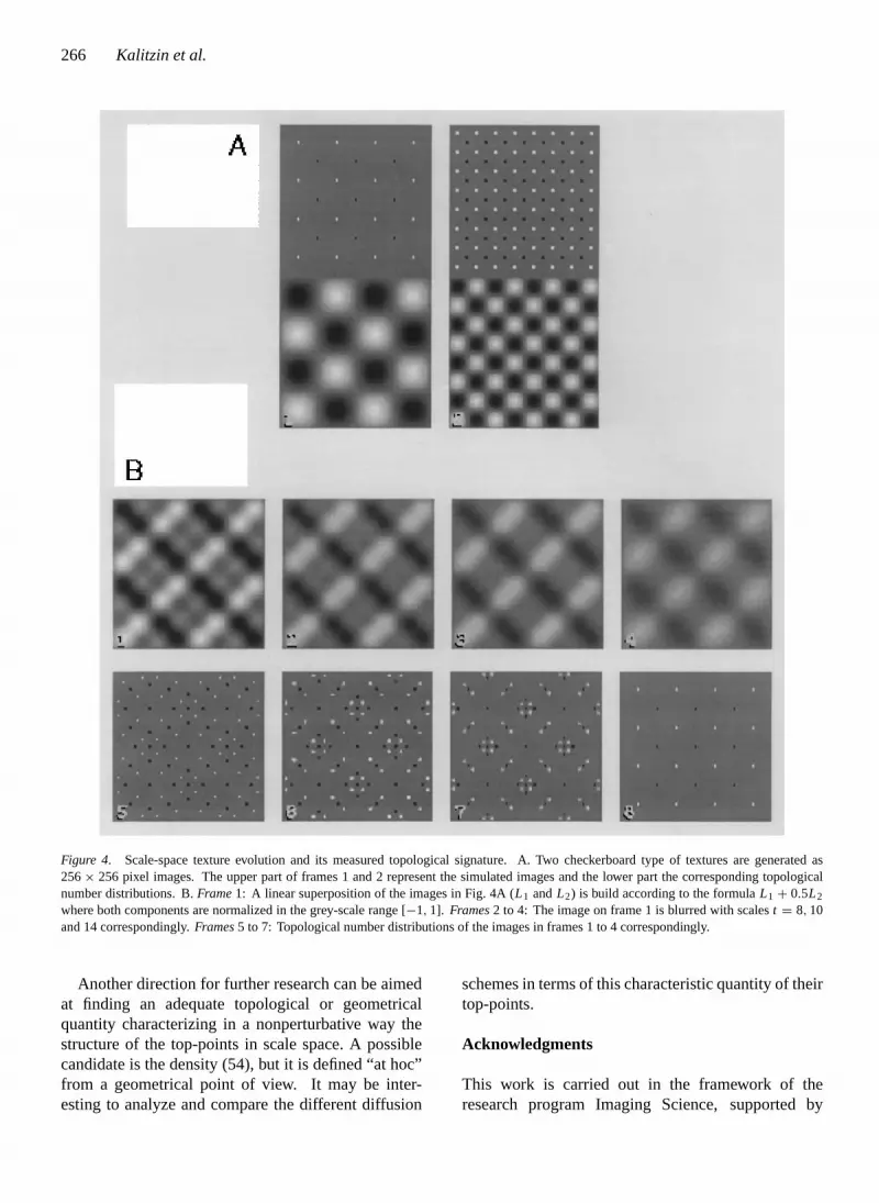
An illustrative example for the localization andscale-evolution properties of the topological numberconsidered in this work is given with Fig. 4. Two tex-ture patterns (check-board images with different wave-length) are superimposed (with different weights) andtheir scale-space evolution is studied.

The first observation we want to stress out from Fig. 4is the nonlinear feature of the invariant (7). Althoughframe 1 Fig. 4B is a linear superposition of the twopatterns in Fig. 4A, the topological number distributionis not. Second, after the Gaussian blurring, the image inframe4 reveals the same topological signature as thedominant texture (the one taken with a larger weight)from frame1 in Fig. 4A. This suggests the possibility ofa scale-classificationof the texture patterns by meansof their topological signatures evolving with scale.

A second applied area, where we can speculate aboutthe use of the topological numbers and their smoothevolution with scale, is the image segmentation realm.As shown in Fig. 5, singularities, localized with theirwinding numbers in a 2D image, determine ahierar-chyof subobjectslabeledby singularities with positivetopological charge (extrema). It is plausible also tosuggest, that at the borders between the subobjects,singularities with negative charge (7) (saddle points)are found. A comprehensivealgorithm for such deep-structure segmentation will involve tracing the objecthierarchy from large, down to finer scales and transfer-ring the object labels to their subobjects. This methodis now under investigation [18] and it involves tech-niques beyond the scope of the current paper.

In this article we used the topological number (7)defined by the normalized gradient vector field. Thesame definition can be directly applied to singularitiesof any vector field. More generally, there are appli-cations where the local orientation structure is definednot by a vector field, but by the Principal directions ofa structural tensor. It would be interesting to extendthe notion of a topological number to those cases. Wewere able to define a winding number associated withthe principle direction in the two-dimensional case.In comparison with the vector winding number consi-dered in Section 3.2, the winding number of the struc-tural tensor is a multiple ofπ . This is due to the factthat the principle direction of the structural tensor hasno orientation on it.



266 Kalitzin et al.

Figure 4. Scale-space texture evolution and its measured topological signature. A. Two checkerboard type of textures are generated as256× 256 pixel images. The upper part of frames 1 and 2 represent the simulated images and the lower part the corresponding topologicalnumber distributions. B.Frame1: A linear superposition of the images in Fig. 4A (L1 andL2) is build according to the formulaL1 + 0.5L2

where both components are normalized in the grey-scale range [−1, 1]. Frames2 to 4: The image on frame 1 is blurred with scalest = 8, 10and 14 correspondingly.Frames5 to 7: Topological number distributions of the images in frames 1 to 4 correspondingly.

Another direction for further research can be aimedat finding an adequate topological or geometricalquantity characterizing in a nonperturbative way thestructure of the top-points in scale space. A possiblecandidate is the density (54), but it is defined “at hoc”from a geometrical point of view. It may be inter-esting to analyze and compare the different diffusion

schemes in terms of this characteristic quantity of theirtop-points.

Acknowledgments

This work is carried out in the framework of theresearch program Imaging Science, supported by




Figure 5. Scale-space evolution of a grey-scale image and its topological signature.Left column: A CT-scan image of 256× 256 pixels isblurred with four different scales.Middle column: The topological number distribution is computed with rectangular contours of size 4 pixels inevery image point.Right column: Combined stack of images representing the scale evolution of the image together with its topological numberdistribution. Extrema (white dots) label blob-type of formations while saddle points (black dots) are situated at the borders of the blobs.

the industrial companies Phillips Medical Systems,KLMA, Shell International Exploration and Produc-tion, and ADAC Europe.

References

1. W.M. Boothby,An Introduction to Differential Geometry andRiemannian Geometry, Academic Press: New York, SanFrancisco, London, 1975.

2. T. Eguchi, P. Gilkey, and J. Hanson, “Gravitation, gauge theo-ries and differential geometry,”Physics Reports, Vol. 66, No. 2,pp. 213–393, 1980.

3. L.M.J. Florack, B.M. ter Haar Romeny, J.J. Koenderink, andM.A. Viergever, “Images: Regular tempered distributions,”in Proc. of the NATO Advanced Research Workshop Shapein Picture—Mathematical Description of Shape in GreylevelImages, Ying-Lie O, A. Toet, H.J.A.M. Heijmans, D.H. Foster,and P. Meer (Eds.), Volume 126 ofNATO ASI Series F, Springer-Verlag: Berlin, 1994, pp. 651–660.



268 Kalitzin et al.

4. P. Johansen, “On the classification of toppoints in scale-space,”Journal of Mathematical Imaging and Vision, Vol. 4, No. 1,pp. 57–68, 1994.

5. M. Kass, A. Witkin, and D. Terzopoulos, “Snakes: Active con-tour models,” inProc. IEEE First Int. Comp. Vision Conf., 1987.

6. J.J. Koenderink, “The structure of images,”Biol. Cybern.,Vol. 50, pp. 363–370, 1984.

7. T. Lindeberg, “Scale-space behaviour of local extrema andblobs,” Journal of Mathematical Imaging and Vision, Vol. 1,No. 1, pp. 65–99, March 1992.

8. T. Lindeberg,Scale-Space Theory in Computer Vision, TheKluwer International Series in Engineering and Computer Sci-ence, Kluwer Academic Publishers: Dordrecht, The Nether-lands, 1994.

9. J. Milnor,Morse Theory, Volume 51 of Annals of MathematicsStudies, Princeton University Press, 1963.

10. M. Morse and S.S Cairns,Critical Point Theory in Global Analy-sis and Differential Topology, Academic Press: New York andLondon, 1969.

11. M. Nakahara,Geometry, Topology and Physics, Adam Hilger:Bristol and New York, 1989.

12. A.H. Salden, “Invariant theory,” inGaussian Scale-Space The-ory, J. Sporring, M. Nielsen, L.M.J. Florack, and P. Johansen(Eds.), Kluwer Academic Publishers, 1997.

13. A.H. Salden, B.M. ter Haar Romeny, and M.A. Viergever, “Lo-cal and multilocal scale-space description,” inProc. of the NATOAdvanced Research Workshop Shape in Picture—MathematicalDescription of Shape in Greylevel Images, Ying-Lie O,A. Toet, H.J.A.M. Heijmans, D.H. Foster, and P. Meer (Eds.),Volume 126 of NATO ASI Series F, Springer-Verlag: Berlin,1994, pp. 661–670.

14. A.H. Salden, B.M. ter Haar Romeny, and M.A. Viergever,“Algebraic invariants of linear scale spaces,”Journal of Mathe-matical Imaging and Vision, March 1996 (submitted).

15. A.H. Salden, B.M. ter Haar Romeny, and M.A. Viergever, “Dif-ferential and integral geometry of linear scale spaces,”Journalof Mathematical Imaging and Vision, May 1996 (submitted).

16. B.M. ter Haar Romeny (Ed.),Geometry-Driven Diffusion inComputer Vision, Kluwer Academic Publishers: Dordrecht,1994.

17. L.M.J. Florack, Detection of Critical Points and Top-Points inScale-Space. In preparation.

18. S.N. Kalitzin, B.M. ter Haar Romeny, and M.A. Viergever,“On topological deep-structure segmentation,” submitted forICIP’97, Santa Barbara.

Stiliyan N. Kalitzin received a master degree in Nuclear Physicsand Nuclear Technology from the University of Sofia, Bulgaria. He

has worked in the Institute for Nuclear Research in Sofia and inthe Joint Institute for Nuclear Research in Dubna, Russia. In 1988he obtained a Ph.D. in Theoretical and Mathematical Physics on thesubjects of Supersymmetry and Supergravity. Since 1990, StiliyanKalitzin hold several consecutive post doctoral positions in differentacademic institutes in the Netherlands. His current research interestsare natural and automated perceptual grouping, neural networks,differential geometry, pattern recognition and nonlinear scale-spacetheories. Since 1996, Stiliyan Kalitzin works in the Image SciencesInstitute at the University of Utrecht.

Bart M. ter Haar Romeny received a M.S. in Applied Physicsfrom Delft University of Technology in 1978, and Ph.D. from UtrechtUniversity in 1983. After being the principal physicist of the UtrechtUniversity Hospital Radiology Department. He joined in 1989 theUtrecht University 3D Computer Vision Research Group where heis an Associate Professor. He is member of the editorial board ofJMIV. His interests are mathematical aspects of front-end vision,in particular, linear and nonlinear scale-space theory, medical com-puter vision applications, picture archiving and communication sys-tems, differential geometry and perception. He authored severalpapers and book-chapters on these issues, edited a recent book onnonlinear diffusion theory in Computer Vision and is involved in(resp. initiated) a number of international collaborations on thesesubjects.

Alfons H. Saldenreceived a M.Sc. in Experimental Physics in 1992and a Ph.D. in 1996 both from utrecht University. His main researchinterests are scale-space theories, invariant theory, differential and in-tegral geometry, theory of partial differential and integral equations,topology and category theory.




Peter FM Nackenhas masters degrees in Mathematics and Theo-retical Physics from the University of Nijmegen, The Netherlands,and a Ph.D. in Computer Science from the University of Amsterdam,

The Netherlands. His research topics included hierarchical methodsfor image segmentation and mathematical morphology. Currently,he is working for Shell International Exploration & Production BV,in the field of 3D seismic interpretation research.

Max A. Viergever

Topological numbers and singularities in scalar images: Scale-space evolution properties

Documents