Topological Mathieu Moonshine - arXiv

arX

iv:2

006.

0292

2v2

[m

ath.

AT

] 1

7 A

pr 2

021

Topological Mathieu Moonshine

Theo Johnson-Freyd

Department of Mathematics, Dalhousie University, Halifax, NS, CANADA

Perimeter Institute for Theoretical Physics, Waterloo, ON, CANADA

E-mail: [email protected]

Abstract: We explore the Atiyah–Hirzebruch spectral sequence for the tmf•[12 ]-cohomology

of the classifying space BM24 of the largest Mathieu group M24, twisted by a class ω ∈H4(BM24;Z[

12 ])

∼= Z3. Our exploration includes detailed computations of the F3-cohomology

of M24 and of the first few differentials in the AHSS. We are specifically interested in the

value of tmf•ω(BM24)[12 ] in cohomological degree −27. Our main computational result is that

tmf−27ω (BM24)[

12 ] = 0 when ω 6= 0. For comparison, the restriction map tmf−3

ω (BM24)[12 ] →

tmf−3(pt)[12 ]∼= Z3 is surjective for one of the two nonzero values of ω.

Our motivation comes from Mathieu Moonshine. Assuming a well-studied conjectural

relationship between TMF and supersymmetric quantum field theory, there is a canonically-

defined Co1-twisted-equivariant lifting [V f] of the class 24∆ ∈ TMF−24(pt), for a specific

value ω of the twisting, where Co1 denotes Conway’s largest sporadic group. We conjecture

that the product [V f]ν, where ν ∈ TMF−3(pt) is the image of the generator of tmf−3(pt) ∼=Z24, does not vanish Co1-equivariantly, but that its restriction to M24-twisted-equivariant

TMF does vanish. We explain why this conjecture answers some of the questions in Mathieu

Moonshine: it implies the existence of a minimally supersymmetric quantum field theory with

M24 symmetry, whose twisted-and-twined partition functions have the same mock modularity

as in Mathieu Moonshine. Our AHSS calculation establishes this conjecture “perturbatively”

at odd primes.

An appendix included mostly for entertainment purposes discusses “ℓ-complexes,” in

which the differential D satisfies Dℓ = 0 rather than D2 = 0, and their relation to SU(2)

Verlinde rings. The case ℓ = 3 is used in our AHSS calculations.

Keywords: supersymmetry, topological modular forms, mock modular forms, sporadic

groups, moonshine, group cohomology, Mathieu group, Steenrod powers, higher complexes.

Contents

1 Introduction 1

1.1 Notation 5

1.2 Acknowledgements 5

2 N = (0, 1) SQFTs 6

2.1 A source of holomorphic anomalies 6

2.2 SQFT• as an Ω-spectrum 11

2.3 Equivariant SQFT• and ’t Hooft anomalies 17

2.4 Twisted and twined shadows 22

2.5 TMF• and tmf• 26

3 Ordinary cohomology of M24 29

3.1 Computing in H•(M24;F3) 30

3.2 Cohomology of P + ǫr acting on H•(M24;F3) 34

4 The Atiyah–Hirzebruch spectral sequence for tmf•ω(BM24) 40

4.1 General comments about AHSSs 40

4.2 Review of tmf•(pt)[12 ] 41

4.3 Differentials for p ≥ 5 43

4.4 Differentials when p = 3 45

4.5 Running the spectral sequence 50

A Higher complexes 54

A.1 ℓ-complexes in characteristic not dividing ℓ 55

A.2 ℓ-complexes in characteristic ℓ 56

1 Introduction

By writing the elliptic genus of an N = (4, 4) K3 sigma model in terms of characters of the

chiral N = 4 superalgebra, Eguchi, Ooguri, and Tachikawa [EOT11] discovered a specific

weight-12 mock modular form (for Γ = SL2(Z)) with shadow 24η(τ)3:

H(τ) = 2q−1/8(−1 + 45q + 231q2 + 770q3 + 2277q4 + . . .

)

Physics readily explains the mock modularity and integrality of H. It does not, however,

explain why the coefficients of H are dimensions of representations of Mathieu’s largest group

M24 [Gan16], and more generally raises the following mysteries:

– 1 –

Question 1.1. Whenever a finite group G acts on a K3 sigma model preserving N = (4, 4)

supersymmetry, the elliptic genus can be twisted and twined by a commuting pair of elements

g, h ∈ G. This produces twisted-twined versions Hg,h(τ) of H(τ) with interesting (mock)

modularity properties, with multiplier that depends on the ’t Hooft anomaly of G. The group

G = M24 does not act nontrivially on any K3 sigma model [GHV12], but nevertheless the

functions Hg,h(τ) exist for all commuting pairs g, h ∈ M24 [GPRV13]. Why?

Question 1.2. A priori, the supertrace in the elliptic genus allows for a large cancelation of

bosonic and fermionic modes. In particular, the coefficients of g 7→ Hg(τ) = He,g(τ) are au-

tomatically virtual characters of G, but have no reason to be honest characters. Nevertheless,

except for the constant term −1, these coefficients are honest characters [Gan16]. Why?

Question 1.3. The functions Hg,h(τ) enjoy a mock-modular analogue of the “genus-zero

property” from monstrous moonshine [CD12]. Why?

The goal of this note is to suggest a solution to Question 1.1. We will not provide a

complete solution—some calculations are too hard—but our suggestion will at least answer

what type of quantum field theory it is that can produce the functions Hg,h(τ). We will

have nothing to say about Question 1.2. We will briefly comment in Conjecture 2.8 about

Question 1.3.

The first step is to recast the problem as a question in stable homotopy theory, and in

particular in elliptic cohomology. This follows the spirit of [Gan09, Tho10] to explain aspects

of moonshine in elliptic cohomological terms, but we believe that many aspects of the specific

approach here are new.

As explained in Section 2, compact minimally supersymmetric (1+1)-dimensional quan-

tum field theories are the cocycles for an extraordinary cohomology theory SQFT•. This

statement is not mathematically rigorous: even the set of “(1+1)-dimensional quantum field

theories” is not mathematically defined (although [ST11] comes close), and topologizing this

set will surely be subtle, but the construction is physically straightforward. This cohomology

theory connects directly with mock modularity [GJF19a]: if S is an SQFT of cohomological

degree 1 − 4k representing the trivial class in SQFT1−4k(pt), then any nullhomotopy of Sdetermines a (generalized) mock modular form with shadow determined by S. We will call

the theory S = ∂F the boundary of its nullhomotopy F . (Note that this is not a “boundary

condition,” where the boundary is on the worldsheet. Rather, it should be thought of as a

boundary in “field space” or “target space,” because if F is a sigma model with target M ,

then ∂F is a sigma model with target ∂M .)

If the boundary SQFT S furthermore admits an action by a finite group G of flavour

symmetries, and if the nullhomotopy is G-equivariant, then the same construction produces

mock modular forms depending on commuting pairs (g, h). The level structure depends on

the orders of g and h, and the multiplier system depends on the ’t Hooft anomaly ω ∈H3(M24; U(1)) ∼= H4(M24;Z) of the G-action. (For the purposes of this introduction, we will

ignore the fact that ’t Hooft anomalies for fermionic QFTs live in “supercohomology” and

– 2 –

not in ordinary cohomology.) In algebrotopological language, the fact that it makes sense

to talk about deformations of SQFTs with G-flavour symmetry and anomaly ω means that

the cohomology theory SQFT• has a twisted equivariant enhancement, allowing us to define

twisted equivariant cohomology groups SQFT•ω(BG) for any finite group G and anomaly

ω ∈ H4(G;Z). Here and throughout, we will write BG for the classifying stack of G; a more

standard name for SQFT•ω(BG) is SQFT•

G,ω(pt).

For example, the direct sum Fer(3)⊕24 of 24 copies of the antiholomorphic supercon-

formal field theory Fer(3) (three antichiral Majorana–Weyl fermions, with supersymmetry

encoding the structure constants of su(2)) is nullhomotopic [GJFW21], and the correspond-

ing mock modular form is H(τ). We can let M24 act on Fer(3)⊕24 by permuting the sum-

mands. Writing 24 for the standard degree-24 permutation representation of M24, we will

call the corresponding M24-equivariant SCFT 24⊗Fer(3). Because the M24-symmetry spon-

taneously breaks to M23, and because H4(M23;Z) = 0, we can think of the M24 action on

24 ⊗ Fer(3)as having any ’t Hooft anomaly that we want (see §2.3). Thus we have classes

[24 ⊗ Fer(3)] = [24] ⊗ [Fer(3)] ∈ SQFT−3ω (BM24) for every ω. If one of them were nullho-

motopic, then the nullhomotopy, with its corresponding mock modular forms, might explain

Mathieu Moonshine.

Unfortunately, we will show in Proposition 2.5 that 24⊗Fer(3) is not M24-equivariantly

nullhomotopic (for any value of the ’t Hooft anomaly). Rather, the boundary SQFT that we

will use is S = V f ⊗ Fer(3), where V f is the holomorphic SCFT constructed in [Dun07].

The automorphism group of V f is Conway’s largest sporadic group Co1, which contains M24

as a subgroup; the computations in [JFT20] show that the anomaly ω of the corresponding

M24-action on S agrees with the anomaly for Mathieu Moonshine computed in [GPRV13].

Cohomological degrees in SQFT• are determined by the central charges of the representing

QFTs, and this S represents a class in cohomological degree −27. Our suggested answer to

Question 1.1 is:

Conjecture 1.4. The antiholomorphic SCFT S = V f ⊗ Fer(3) represents the trivial class

[S] = 0 in SQFT−27ω (BM24).

Without further information about SQFT•, it seems impossible to test this conjecture.

But in fact there is a rather clear idea of the structure of SQFT•, with evidence continuing

to amass [Seg88, HK04, ST04, Che06, Seg07, ST11, BE15, BE16, BET18, GJF21, BET19,

GJFW21, GJF19a] in favour of the following conjecture:

Conjecture 1.5. The spectrum SQFT• represents the universal elliptic cohomology theory

TMF• of “topological modular forms” described in [Lur09, DFHH14].

Under this equivalence, the class [Fer(3)] ∈ SQFT−3(pt) corresponds to the class usually

denoted ν ∈ TMF−3(pt) = π3TMF, the image under the Hurewicz map of the 3-sphere

S3 = SU(2) with its Lie group framing [GJFW21], and the class [V f] ∈ SQFT−24(pt) is

24∆ ∈ TMF−24(pt) [GJF21], where ∆ = (c34 − c26)/1726 is the usual modular discriminant.

(The curly braces around 24∆ are there because ∆ itself is not a class in TMF−24(pt).)

– 3 –

Recently a complete definition of equivariant TMF has become available [Lur19, GM20].

Assuming Conjecture 1.5, Conjecture 1.4 becomes:

Conjecture 1.6. There is a distinguished refinement of 24∆ ∈ TMF−24(pt) to a class

in TMF−24ω (BCo1), and, after multiplying by ν and restricting along M24 ⊂ Co1, the class

24∆ν vanishes in TMF−27ω (BM24).

Note that the M24-action on V f, and hence on S = V f ⊗ Fer(3), extends to a Co1-

action. However, we do not believe that [S] = 24∆ν vanishes Co1-equivariantly. It is worth

emphasizing that, in order to define 24∆ν ∈ TMF−27ω (BM24), one would need to show that

the nonequivariant class 24∆ ∈ TMF−24(pt) admits an equivariant refinement to a class

in TMF−24ω (BCo1). The existence of such a refinement is implied by Conjecture 1.5, but it

has not been shown mathematically rigorously. Furthermore, in §2.5 we will suggest that an

answer to Question 1.3 might come from proving:

Conjecture 1.7. 24∆ refines to a class in Tcf−24ω (BCo1), the space of (twisted) Co1-

equivariant topological cusp forms, and the restriction of 24∆ν vanishes in Tcf−27ω (BM24).

Unfortunately, this author is not aware of techniques for computing twisted equivariant

TMF• (let alone Tcf•) groups. Instead, as evidence in favour of Conjecture 1.6, we will

attempt to compute the related group tmf−27ω (BM24). There are two changes involved. First,

we have replaced the genuinely equivariant problem with the Borel-equivariant one. Any

group G has a classifying space BG, and for any cohomology theory E•, Borel-equivariant E•-

cohomology studies cohomology of BG in place of BG. As with Atiyah–Segal completion for

K-theory [AS04, AS06], one expects in general that E•(BG) is an approximation of E•(BG),

but the latter may include more information than the former. (In fact, the “completion”

story for TMF is subtle, and typically fails for Lie groups [GM20], but seems to hold for

finite groups.) Second, we have replaced the spectrum TMF• by the related spectrum tmf•.

Speaking very roughly (see §2.5 for an important correction), tmf• corresponds to the modular

forms which are bounded at the cusp τ = i∞ and TMF• corresponds to the modular forms

which are meromorphic at the cusp; on homotopy groups, TMF•(pt) = tmf•[∆−24], and if

a class in tmf• vanishes, then its image in TMF• also vanishes. There is no known physical

description of tmf•, and there is not expected to be one.

Actually, computing tmf•ω(BM24) is still too hard, because the 2-local structure of tmf•

is complicated and the 2-local cohomology of M24 is not known. So we will attempt only

tmf•ω(BM24)[12 ]. After further inverting 3, the spectrum tmf•[16 ] becomes the spectrum called

“Eℓℓ” in [Tho94], where it is shown that tmf•ω(BM24)[16 ] (which is independent of ω) is

supported only in even degrees. As such, our computation is interesting only at the prime 3.

After a detailed study of H•(M24;F3) in Section 3, in Section 4 we investigate the Atiyah–

Hirzebruch spectral sequence for tmf•ω(BM24)[12 ]. Note that we are particularly interested in

the groups tmf−27ω (BM24), which houses the image under the completion map tmf(BM24) →

tmf(BM24) of the equivariant enhancement of 24∆ν, and tmf−3ω (BM24), which houses the

image under completion of 24ν. Our main mathematical result is:

– 4 –

Theorem 1.8. If ω ∈ H4(M24;Z[12 ])

∼= Z3 is nonzero, then tmf−27ω (BM24) = 0. For com-

parison, for one of the two nonzero values of ω, and not the other one, the restriction map

tmf−3ω (BM24)[

12 ] → tmf−3(pt)[12 ] is nonzero.

Spectral sequences in general, and the Atiyah–Hirzebruch spectral sequence in particular,

are the homotopy algebraist’s version of perturbation theory. Indeed, a physicist should think

of the difference between TMF•ω(BG) and TMF•

ω(BG) as the difference between nonperturba-

tive and perturbative field theory. One can pull back along the map BG→ BG to produce a

map TMF•ω(BG) → TMF•

ω(BG). The domain, hypothetically, encodes deformation classes of

SQFTs with G-flavour symmetry, and in particular their behaviours on worldsheets equipped

with arbitrary G-bundle, whereas the codomain remembers only the physics “near the trivial

G-bundle.” (Since G is finite, the stack of G-bundles has no perturbative structure “over C,”

but it does have perturbative structure p-locally for any prime p dividing the order of G.)

To end the paper, Appendix A describes some of the theory of “chain complexes” in which

the “differential” does not satisfy D2 = 0 but rather Dℓ = 0 for ℓ > 2. Some of this theory,

for ℓ = 3, is important in our calculations. The larger story connects in intriguing ways to

the Verlinde ring for SU(2) at level k = ℓ− 2, and some readers may find it entertaining.

1.1 Notation

We will write Zn for the cyclic group of order n. This name is reasonably standard in

the physics literature; mathematicians may prefer Cn or Z/nZ. For other finite groups, we

generally follow ATLAS naming conventions [CCN+85]. For a prime p, we will write Z(p)

for the ring of p-local integers, i.e. the subring of Q consisting of fractions with denominator

coprime to p. The finite field with q = pn elements is Fq; a generic field is K.

We will always use cohomological degree conventions, with degrees always written as

superscripts. For example, the homotopy groups of a spectrum E• are E•(pt) = π0E• = π−•E .If E• is connective (e.g. tmf•), then these groups are supported in nonpositive cohomological

degree. Without care, this paper would devolve into alphabet soup. So, for example, Bock-

stein maps will be denoted rather than β. We will sometimes write the group cohomology

of a finite group G, with coefficients in an abelian group A, as H•(G;A), and sometimes

as H•(BG;A), with “BG” denoting the classifying space of G. For an extraordinary coho-

mology theory E•, we will always use the latter name: E•(BG) is the E•-cohomology of the

space BG. If E• also admits an equivariant refinement, then we can evaluate E• on the clas-

sifying stack BG of G; by definition E•(BG) = E•G(pt) is the G-equivariant cohomology of a

point. When E• = H•(−;A) is ordinary cohomology, the groups H•(BG;A) and H•(BG;A)

agree, justifying our use of simply H•(G;A).

1.2 Acknowledgements

I thank D. Berwick-Evans for detailed and helpful comments on a draft of this paper. Sec-

tions 2.1 and 2.2 are based on ideas developed by the author jointly with D. Gaiotto, whom

I thank for ongoing discussions about this circle of ideas. Research at Perimeter Institute

– 5 –

is supported in part by the Government of Canada through the Department of Innovation,

Science and Economic Development Canada and by the Province of Ontario through the

Ministry of Colleges and Universities. The Perimeter Institute is in the Haldimand Tract,

land promised to the Six Nations. Dalhousie University is in Mi‘kma‘ki, the ancestral and

unceded territory of the Mi‘kmaq.

2 N = (0, 1) SQFTs

The goal of this section is to describe a detailed but largely conjectural relationship between

elliptic cohomology, mock modularity, and supersymmetry. As such, the language will drift

between mathematics and theoretical physics, and we will leave some statements mathemat-

ically imprecise. Sections 3 and 4 consist of rigorous mathematical calculations motivated by

the conjectures in this section.

2.1 A source of holomorphic anomalies

The starting point of our analysis is the following question: What type(s) of quantum field

theories produce mock modular forms? The (an?) answer has been well-investigated for more

than a decade [EST07, MM10, Tro10, ES11, Sug12, Mur14, ADT14, GM17, GJF19a, DJR19,

Sug20, DPW20]: A (1+1)-dimensional quantum field theory can produce mock modular

instead of modular forms if it is noncompact.

We will not in this paper attempt to define “quantum field theory.” We will always assume

our QFTs to be unitary, so that we have access to Wick rotation to Euclidean signature

(imaginary time). The physics literature does not seem to include a complete definition of

“compactness” for a QFT, but the consensus is that it should be a “spectral condition,”

since in the case of sigma-models what distinguishes compact from noncompact target is that

the former lead to Hamiltonians with discrete spectrum, whereas the latter have continuous

spectrum. We propose the following: a (d+1)-dimensional QFT is compact if its Wick-

rotated partition function “converges absolutely” on all closed spacetimes: in Lagrangian

formalism, we imagine an “absolutely convergent path integral” (in spite of the fact that not

all QFTs have path integral descriptions, and most spaces of fields do not support measures

of integration in the mathematical sense); in Hamiltonian formalism, we are asking that the

Wick-rotated evolution operator tr(exp(−τH)) should be trace-class. This latter condition

occurs when the spectrum of the Hamiltonian H is bounded below, discrete, and does not

grow too slowly. Compactness is a nontopological version of asking whether a functorial

topological field theory is defined on all cobordisms, or if it is only partially defined.

Badly noncompact QFTs might even fail to assign Hilbert spaces of states to all closed d-

dimensional spaces. The most mild type of noncompactness is when the Hilbert spaces are all

well-defined, but the Wick-rotated partition function converges only conditionally. The value

of a conditionally-convergent sum or integral can depend on the method used to evaluate it,

and so the partition function of a mildly noncompact QFT is not quite well-defined. This is the

– 6 –

origin of phenomena like mock modularity in noncompact QFTs: modular transformations

may not be compatible with the chosen evaluation method.

Focusing on the case we care most about, let F be a (1+1)-dimensional QFT, and write

Z(F) for its partition function on flat oriented 2-dimensional tori (these being the only flat

closed oriented 2-manifolds). If F has fermions, then Z(F) depends on a choice of spin

structure on the worldsheet. We will care most about the case of nonbounding spin structure,

which is to say the Ramond spin structure along both the A- and B-cycles; we will thus call

this the “Ramond-Ramond” partition function ZRR(F). The space of flat tori (with RR spin

structure) is 3-real dimensional: the local coordinates are the complex structure (τ, τ) and the

area a. If F is compact, then Z(F) is a well-defined function of these three real variables, and

we assume that it is real-analytic. (As with essentially all analytic questions about QFT, this

is an assumption, and we must fold it into some aspect of the definition of “compact QFT.”)

Because different values of (τ, τ , a) describe the same torus, a 7→ ZRR(τ, τ , a) is a real-analytic

family of real-analytic SL2(Z)-modular functions. In the conformal case, of course, there is

no a-dependence.

Now suppose that F is not just a compact QFT, but also is equipped with an N = (0, 1)

supersymmetry. A standard argument then says that ZRR(F) depends only on τ [Wit87].

This argument is so familiar that we will not review it, except to make a few comments:

1. The statement only holds in the Ramond-Ramond spin structure.

2. Let Q denote the supercurrent for the N = (0, 1) supersymmetry. (It is usually called

“G,” but we will soon want the letter G to stand for a finite group.) This supercurrent is

a worldsheet spinor, and so has two components, which explain the two nondependencies

(on τ and on a). Given coordinates z, z on the worldsheet, we can write the two

components of Q as Qz and Qz. The former is the “trace” of Q, and vanishes if F is

superconformal.

3. The growth rate of ZRR(F)(τ) as τ → i∞ is not worse than exp(τ2c/24), where c is

the central charge of F , and τ2 = (τ − τ)/2i is the imaginary part of τ . As such,

ZRR(F)(τ) is a weakly holomorphic modular function, meaning a modular function

which is holomorphic for finite τ , and meromorphic at the cusp τ = i∞.

4. F has a gravitational anomaly if its left and right central charges cL, cR do not match.

The difference w = cR − cL is always a half-integer. When w 6= 0, ZRR(F) suffers a

multiplier under T -transformations:

T [ZRR(F)] = e−w2πi24 ZRR(F).

This multiplier can be absorbed by adjusting

ZRR(F) Z ′RR(F) = ZRR(F)η(τ)2w .

This adjusted partition function Z ′RR(F) is then a weakly holomorphic modular form of

weight w and trivial multiplier. It matches better with the mathematics conventions for

– 7 –

Witten genera. In [GJF19a], this adjustment (up to a factor of iw that we will ignore)

is interpreted in terms of “spectator” Majorana–Weyl fermions that are added to F to

cure the anomaly. In §2.2 we will interpret the integer n = −2w as the cohomological

degree of F .

5. The q-expansion of ZRR(F) is the index of the S1-equivariant supersymmetric quantum

mechanics model H(F) formed by compactifying F on an A-cycle with Ramond spin

structure, thus explaining why ZRR(F) ∈ Z((q)). The q-expansion of Z ′RR(F) is built

by adjusting the SQM model by some spectator fermions.

When F is not compact, the standard arguments can break down, as we have already

indicated. Following [GJF19a], we will focus on a particularly mild noncompactness, which

is when F has “cylindrical ends.”

In order to give the definition, we will need the following construction. Let Φ be a

self-adjoint operator in the SQFT F , thought of as a “function” Φ : F → R. There is a

straightforward way to construct the “fibre” of Φ over x ∈ R, which we will denote F(Φ =

x), or F(x) when Φ is implicit. Namely, add to F a chiral Majorana–Weyl fermion λ,

which will serve as a Lagrange multiplier, to produce the QFT F ⊗ Fer(1). Now deform the

supersymmetry on F ⊗ Fer(1) by adding a superpotential equal to

W = λ(Φ− x).

This results in an adjustment of the Lagrangian like λQ[Φ − x] + (Φ − x)2. In the IR, one

expects this F(Φ = x) to flow to an SQFT in which Φ takes the constant value x.

Conversely, one expects to be able to recover F from the R-family of SQFTs x 7→ F(Φ =

x) by dynamicalizing the parameter x. This dynamicalization procedure involves replacing

the parameter x by a scalar field φ and also introducing its (right-moving) superpartner ψ,

so that together (φ,ψ) is a scalar supermultiplet for the N = (0, 1) algebra. We will write

the result of this dynamicalization as

F(x) 7→∫

φ,ψF(φ).

The SQFT F is then said to have cylindrical ends if it can be equipped with a Φ such

that the SQFTs F(x) are all compact, and if supersymmetry is spontaneously broken when

x ≪ 0, and if the theories F(x) stabilize to some fixed SQFT ∂F when x ≫ 0. We will call

∂F the boundary of F . Note that this is a boundary in field space, and not a “boundary

condition” that can be assigned to boundaries of the worldsheet.

For example, if F consists of a massless scalar φ (i.e. a noncompact nonchiral boson),

together with its superpartner ψ (an antichiral Majorana–Weyl fermion), and if Φ = φ2, then

F(x) picks up a quartic potential (φ2 − x)2 and a Yukawa coupling λφψ. If x < 0, F(x)

has spontaneous supersymmetry breaking, whereas if x > 0, F(x) has two massive vacua,

with fermion masses of opposite signs, and so the two vacua differ by a relative Arf invariant

– 8 –

(c.f. §2.1.1 of [KPMT19]). After fixing a convention about fermion masses (as in [KTT19,

Section 2], for example), we see that the noncompact scalar multiplet, i.e. the sigma-model

with target R, has cylindrical boundary equal to (trivial TQFT)⊕ (Arf TQFT).

Suppose that F has cylindrical ends, parameterized by an operator Φ. Then the partition

function of F has no reason to converge absolutely. But if the partition function of the

boundary vanishes,

ZRR(∂F) = 0,

then one expects that the path integral description of ZRR(F) will converge conditionally,

because the end R≫0×∂F contributes a term like 0×vol(R≫0), which we take to be 0. In this

way we can define ZRR(F). (The value of ZRR(F) might depend on the parameterization Φ.)

Because we never chose coordinates on the worldsheet, ZRR(F)(τ, τ , a) is manifestly

SL2(Z)-modular, and we will assume that it is real-analytic. However, it is not automat-

ically holomorphic, because the standard argument for holomorphicity requires compact-

ness. Rather, ZRR(F)(τ, τ , a) can suffer a holomorphic anomaly. One of the main results

of [GJF19a] is a precise formula for this holomorphic anomaly. The justification given in that

paper is a combination of heuristic arguments about path integrals and applying Stokes’ for-

mula in field space, together with carefully-worked examples to fix the proportionality factors.

A more detailed proof in the case of sigma models is given in [DPW20]. But in the general

case the arguments from [GJF19a] would need further improvements in order to provide a

“theorem” even at physicists’ level of rigour, and so we will call it here a “conjecture”:

Conjecture 2.1 ([GJF19a]). Suppose F is an N = (0, 1) SQFT with cylindrical ends and

boundary ∂F , and that ZRR(∂F) = 0. Then deformations of F that are “compactly sup-

ported,” i.e. that don’t deform the end F≫0, do not effect the value of ZRR(F). Moreover, the

τ - and a-dependence of the conditionally convergent partition function ZRR(F)(τ, τ , a) are de-

termined entirely by the boundary ∂F . In particular, if ∂F is superconformal, then ZRR(∂F)

has no a-dependence, and its τ -dependence is governed by the holomorphic anomaly equation

(up to convention-dependent factors of 4√−1):

√−8τ2η(τ)

∂

∂τZRR(F) = (torus one-point function of Qz in ∂F)

Thus, if ∂F is superconformal, the adjusted partition function Z ′RR(F) = ZRR(F)η(τ)w

is a real-analytic, but not holomorphic, modular form of weight w, where w = cR − cL is the

gravitational anomaly of F . Any real-analytic modular form f(τ, τ ) has a holomorphic part

f(τ), defined by analytically continuing and then taking a limit

f(τ) = limτ→−i∞

f(τ, τ),

assuming the limit exists. This is an example of a generalized mock modular form, with

shadow the complex conjugate of√−8τ2

∂f∂τ . (An excellent reference on many aspects of mock

modularity is [BFOR17].) It is honestly mock modular if the shadow is (weakly) holomorphic.

– 9 –

In particular, suppose that ∂F is a purely antiholomorphic SCFT (i.e. all of its fields are

antichiral). Then the torus one-point function of Q = Qz is antiholomorphic, and so

f(τ) = η(τ) limτ→−i∞

ZRR(F)(τ, τ )

will be a weight-1/2 mock modular form (with multiplier), and shadow (the complex conjugate

of) the torus one-point function of Q in ∂F .

The analysis in [GJF19a] furthermore suggests:

Conjecture 2.2 ([GJF19a]). Suppose that F as in Conjecture 2.1, with ∂F superconformal.

Then the holomorphic part of ZRR(F) exists (the limit converges). Its q-expansion is the index

of the S1-equivariant SQM model H(F) formed by compactifying F on an appropriate Ramond

circle called the Tate curve. (The compactification explicitly breaks SL2(Z)-modularity.) This

index lives in Z((q)) up to a correction given by an Atiyah–Patodi–Singer invariant of ∂F .

Because of the extra time-reversal symmetry of H(F) (c.f. §3.2.2 of [GPPV18]), this APS

invariant is just a half-integer related to a certain “mod-2 index” of ∂F .

The following example was the primary motivation for [GJFW21, GJF19a]. Take a K3

surface with 24 punctures, and arrange a B-field on M so that its flux near each puncture

satisfies∫S3 H/2π = 1. Now form an N = (0, 1) sigma model with target this noncompact 4-

manifold. (The (0, 1) worldsheet supersymmetry enhances to (0, 4) by using the hyperkaahler

structure. The B-field is needed to cancel an anomaly that would otherwise be present because

of the mismatched fermions [MN85].) The result is a noncompact SCFT F with cylindrical

ends. The boundary theory ∂F = Fer(3)⊕24 is a direct sum of 24 copies of the same theory, one

for each puncture. The contribution from each puncture is a purely antiholomorphic SCFT

Fer(3) consisting of three antichiral Majorana–Weyl fermions ψ1, ψ2, ψ3 and supersymmetry

G = :ψ1ψ2ψ3:, up to convention-dependent factors of 4√−1. The torus one-point function

of G in each summand is η(τ )3. Thus the K3 surface produces a mock modular form with

shadow 24η(τ)3, namely the function H(τ) that we started with in Section 1.

Fer(3)⊕24 is not the only possible boundary theory for producing H(τ), and is not the

one we will end up using. There is a famous holomorphic SCFT called V f constructed

in [Dun07], with automorphism group Aut(V f) = Co1 and central charge cL = 12 (and

cR = 0). We will work instead with its reflection to an antiholomorphic SCFT V f. The

supersymmetry together with the antiholomorphicity imply that the Ramond-sector partition

function ZRR(V f) simply counts the Ramond-sector ground states, of which there are 24.

Thus the torus one-point function of Q in V f ⊗ Fer(3) is

〈Q〉V f⊗Fer(3)

= 〈1〉V f 〈Q〉Fer(3) + 〈Q〉

V f 〈1〉Fer(3) = 24η(τ )3 + 0.

As we will explain in §2.5, Conjecture 1.5 implies that V f ⊗ Fer(3) is a boundary of an

N = (0, 1) SQFT F with cylindrical ends, thus providing another source of mock modular

forms with shadow 24η(τ)3.

– 10 –

2.2 SQFT• as an Ω-spectrum

The story in the previous section applies in the presence of a finite group G of flavour symme-

tries. Namely, suppose that F is a noncompact SQFT with cylindrical ends ∂F and G-flavour

symmetry. After averaging, we may assume that Φ is G-invariant. Then G acts on ∂F , and

so the right-hand side of the holomorphic anomaly equation 2.1 may be twisted and twined by

elements of G, and we predict that it will be the holomorphic anomaly for the corresponding

twisted-twined partition function of F . After taking holomorphic parts, we would produce a

(generalized) mock modular form valued in characters of G.

Thus we can answer Question 1.1 if we can produce an SQFT S which is not just the

boundary of an SQFT F with cylindrical ends, but is such a boundary compatibly with an

M24-flavour symmetry. By exchanging F with the R-family x 7→ F(x), we are equivalently

asking whether S can be deformed continuously, in an M24-equivariant way, to an SQFT with

spontaneous supersymmetry breaking: whether S is in the “spontaneous-supersymmetry-

breaking phase” of SQFTs with M24 flavour symmetry, or whether its supersymmetry is

“protected” by the M24-symmetry.

This question—whether some object can be continuously deformed into some other

object—is the fundamental question of homotopy theory, and we will try to answer it by

adopting homotopical techniques. Specifically, we will see that the space of SQFTs is not

merely a topological space, but rather has extra structure making it into a “spectrum.” The

algebraic topology of spectra is more rigid than the algebraic topology of spaces, and there

are more tools available. The construction of a spectrum SQFT• described in this section is

closely related to a construction in [BE16] (see also [ST04, ST11, DH11]).

In order to describe this spectrum structure, we will need to discuss in a bit more detail

the gravitational anomalies that (1+1)-dimensional (S)QFTs can enjoy. Specifically, we will

distinguish two versions of the word “quantum field theory,” which we call “absolute” versus

“anomalous.” For related recent discussion, see e.g. [Fre19, JF20].

For a QFT to be absolute, it must come with extra data which is of debatable physical

content. An absolute QFT has an absolutely-defined partition function, with no ambiguity

about, say, the “zero” in the energy scale, or about the normalization of the path integral

measure. An absolute QFT should have well-defined (super) Hilbert spaces, with no projec-

tivity in the action by isometries: vectors in this Hilbert space have well-defined phases. Since

the partition function is part of the data of an absolute QFT, symmetries of absolute QFTs

never have ’t Hooft anomalies. The group of symmetries of an absolute quantum mechanics

model is a subgroup of the unitary group rather than the projective unitary group. The usual

functorial definition of topological QFTs, building on the original definition of [Ati88], is an

attempt to model absolute TQFTs.

For comparison, an anomalous QFT is one that tolerates many phase ambiguities in its

values. To tolerate an ambiguity in the meaning of “zero” energy, anomalous QFTs have

“partition functions” that are not functions, but rather sections of possibly-nontrivial line

bundles. To tolerate an ambiguity in the phase of a pure state, anomalous QFTs assign

– 11 –

projective Hilbert spaces rather than honest Hilbert spaces. Symmetries of anomalous QFTs

typically have nontrivial ’t Hooft anomalies. QFTs defined in terms of their algebras of

operators are typically anomalous, and more data would to be needed in order to promote

them to absolute QFTs. The simplest example of this is the Stone–von Neumann theorem,

which says that an algebra of observables determines the Hilbert space functorialy only up

to a phase ambiguity, i.e. only as a projective Hilbert space.

In the case of (1+1)-dimensional QFTs, the obstruction to promoting from anomalous to

absolute is the gravitational anomaly w = cR−cL mentioned in §2.1. If this anomaly vanishes,

then there are still choices. For fermionic QFTs, it turns out that there are two choices (up to

isomorphism), which differ by the parity of the Ramond-sector Hilbert space. (The parity of

the Neveu–Schwarz sector is fixed by the state-operator correspondence.) There are further

anomalies and choices if one wants to promote from anomalous to absolute in the presence of

a symmetry. For example, symmetries of the operator algebra typically act only projectively,

or more precisely via a spin lift, on the Ramond-sector, and there is the standard ’t Hooft

anomaly cocycle. All together, the space of anomalies for fermionic (1+1)-dimensional QFTs

is the 4-layer spectrum described in §5.6 of [GJF19b] with homotopy groups Z,Z2,Z2, 0,Z.

This spectrum is called “fGP×≤4” in [GJF19b], and the convention in that paper is that the

homotopy groups live in degrees

(fGP×≤4)

3(pt) = Z, (fGP×≤4)

2(pt) = Z2, (fGP×≤4)

1(pt) = Z2,

(fGP×≤4)

0(pt) = 0, (fGP×≤4)

−1(pt) = Z,

where by definition (fGP×≤4)

•(pt) = π−•fGP×≤4, and, as mentioned already in §1.1, we will

try always to use cohomological degree conventions. The gravitational anomaly itself lives

(after multiplication by 2, since cR − cL is a half-integer) in the Z in cohomological degree

3 = (1+1) + 1, and the Z2 in cohomological degree 2 corresponds to the two choices for

promoting a QFT with vanishing gravitational anomaly to an absolute QFT.

The simplest example of a (1+1)-dimensional QFT whose gravitational anomaly does not

vanish is the theory Fer(1) of a single chiral Majorana–Weyl fermion. This is a holomorphic

conformal field theory, with central charges cL = 12 and cR = 0. It can be made into an

N = (0, 1) superconformal field theory by declaring that the supersymmetry operator acts

trivially. Since cR 6= cL, this SCFT cannot be promoted to an absolute QFT. For example,

its “partition function” is not a function, but rather a section of a nontrivial line bundle

on the moduli space of spin Riemann surfaces called the Pfaffian line [Fre87, Bor92]. (It

is in fact best thought of as a bundle of superlines, with fibres isomorphic either to C1|0 or

C0|1 depending on whether the spin Riemann surface is or is not the boundary of a spin

3-manifold.) The tensor product (aka stacking) of n copies of Fer(1) produces an N = (0, 1)

SCFT Fer(n) = Fer(1)⊗n with (cL, cR) = (n2 , 0).

Definition 2.3. SQFTn is the space of compact unitary N = (0, 1) SQFTs whose anomaly

is identified with the anomaly for Fer(n).

– 12 –

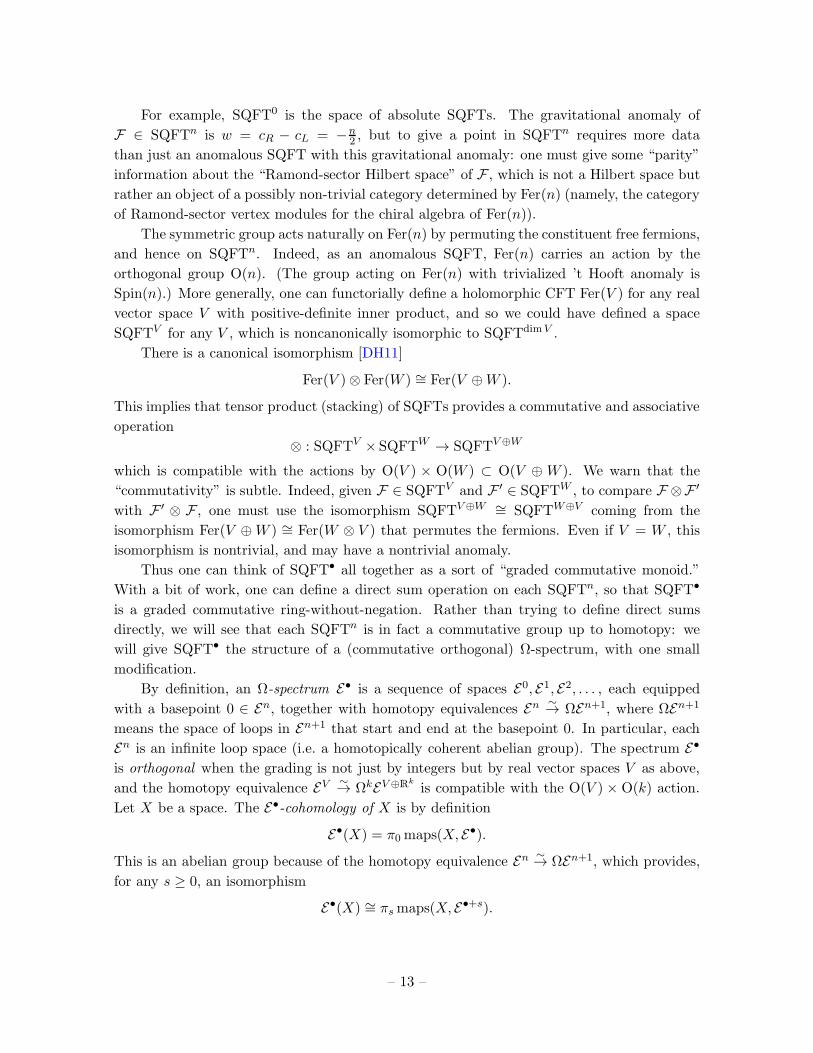
For example, SQFT0 is the space of absolute SQFTs. The gravitational anomaly of

F ∈ SQFTn is w = cR − cL = −n2 , but to give a point in SQFTn requires more data

than just an anomalous SQFT with this gravitational anomaly: one must give some “parity”

information about the “Ramond-sector Hilbert space” of F , which is not a Hilbert space but

rather an object of a possibly non-trivial category determined by Fer(n) (namely, the category

of Ramond-sector vertex modules for the chiral algebra of Fer(n)).

The symmetric group acts naturally on Fer(n) by permuting the constituent free fermions,

and hence on SQFTn. Indeed, as an anomalous SQFT, Fer(n) carries an action by the

orthogonal group O(n). (The group acting on Fer(n) with trivialized ’t Hooft anomaly is

Spin(n).) More generally, one can functorially define a holomorphic CFT Fer(V ) for any real

vector space V with positive-definite inner product, and so we could have defined a space

SQFTV for any V , which is noncanonically isomorphic to SQFTdimV .

There is a canonical isomorphism [DH11]

Fer(V )⊗ Fer(W ) ∼= Fer(V ⊕W ).

This implies that tensor product (stacking) of SQFTs provides a commutative and associative

operation

⊗ : SQFTV × SQFTW → SQFTV⊕W

which is compatible with the actions by O(V ) × O(W ) ⊂ O(V ⊕ W ). We warn that the

“commutativity” is subtle. Indeed, given F ∈ SQFTV and F ′ ∈ SQFTW , to compare F ⊗F ′

with F ′ ⊗ F , one must use the isomorphism SQFTV⊕W ∼= SQFTW⊕V coming from the

isomorphism Fer(V ⊕W ) ∼= Fer(W ⊗ V ) that permutes the fermions. Even if V = W , this

isomorphism is nontrivial, and may have a nontrivial anomaly.

Thus one can think of SQFT• all together as a sort of “graded commutative monoid.”

With a bit of work, one can define a direct sum operation on each SQFTn, so that SQFT•

is a graded commutative ring-without-negation. Rather than trying to define direct sums

directly, we will see that each SQFTn is in fact a commutative group up to homotopy: we

will give SQFT• the structure of a (commutative orthogonal) Ω-spectrum, with one small

modification.

By definition, an Ω-spectrum E• is a sequence of spaces E0, E1, E2, . . . , each equipped

with a basepoint 0 ∈ En, together with homotopy equivalences En ∼→ ΩEn+1, where ΩEn+1

means the space of loops in En+1 that start and end at the basepoint 0. In particular, each

En is an infinite loop space (i.e. a homotopically coherent abelian group). The spectrum E•

is orthogonal when the grading is not just by integers but by real vector spaces V as above,

and the homotopy equivalence EV ∼→ ΩkEV⊕Rkis compatible with the O(V ) × O(k) action.

Let X be a space. The E•-cohomology of X is by definition

E•(X) = π0 maps(X, E•).

This is an abelian group because of the homotopy equivalence En ∼→ ΩEn+1, which provides,

for any s ≥ 0, an isomorphism

E•(X) ∼= πsmaps(X, E•+s).

– 13 –

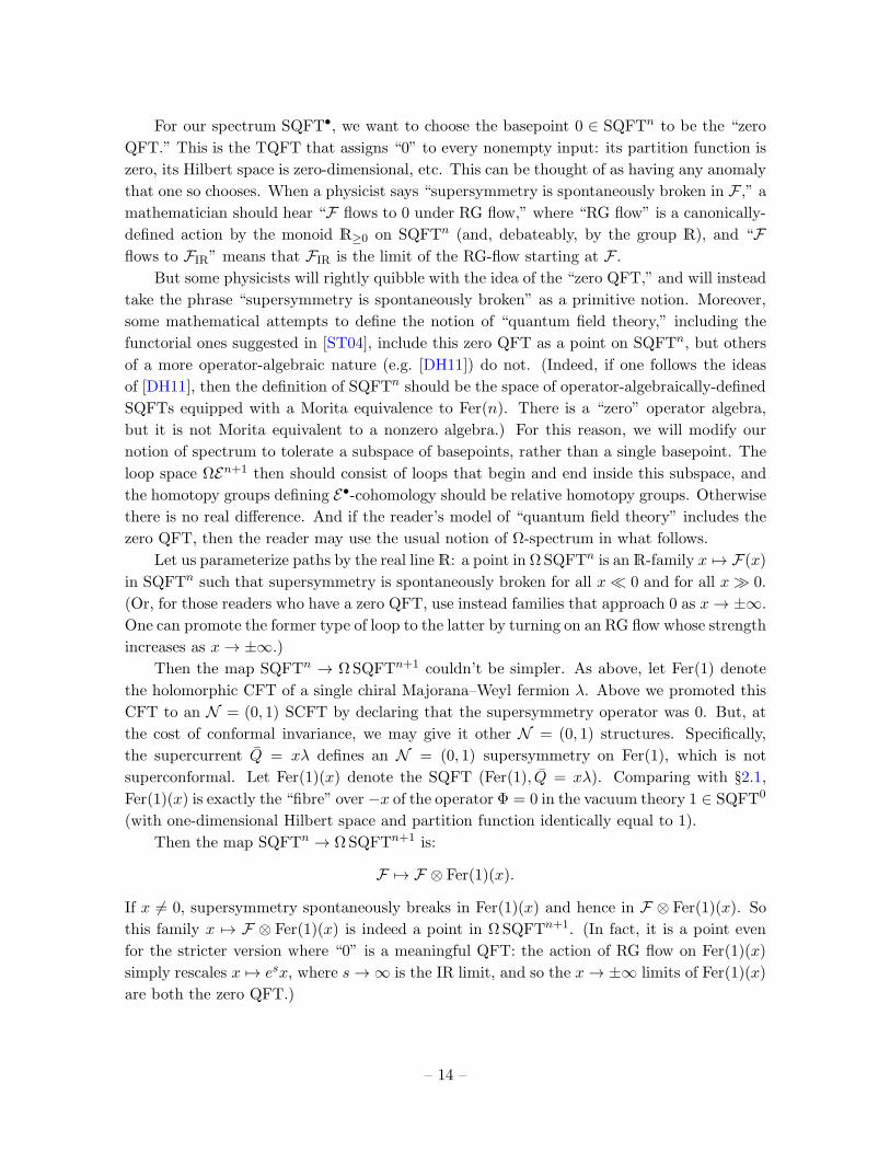
For our spectrum SQFT•, we want to choose the basepoint 0 ∈ SQFTn to be the “zero

QFT.” This is the TQFT that assigns “0” to every nonempty input: its partition function is

zero, its Hilbert space is zero-dimensional, etc. This can be thought of as having any anomaly

that one so chooses. When a physicist says “supersymmetry is spontaneously broken in F ,” a

mathematician should hear “F flows to 0 under RG flow,” where “RG flow” is a canonically-

defined action by the monoid R≥0 on SQFTn (and, debateably, by the group R), and “Fflows to FIR” means that FIR is the limit of the RG-flow starting at F .

But some physicists will rightly quibble with the idea of the “zero QFT,” and will instead

take the phrase “supersymmetry is spontaneously broken” as a primitive notion. Moreover,

some mathematical attempts to define the notion of “quantum field theory,” including the

functorial ones suggested in [ST04], include this zero QFT as a point on SQFTn, but others

of a more operator-algebraic nature (e.g. [DH11]) do not. (Indeed, if one follows the ideas

of [DH11], then the definition of SQFTn should be the space of operator-algebraically-defined

SQFTs equipped with a Morita equivalence to Fer(n). There is a “zero” operator algebra,

but it is not Morita equivalent to a nonzero algebra.) For this reason, we will modify our

notion of spectrum to tolerate a subspace of basepoints, rather than a single basepoint. The

loop space ΩEn+1 then should consist of loops that begin and end inside this subspace, and

the homotopy groups defining E•-cohomology should be relative homotopy groups. Otherwise

there is no real difference. And if the reader’s model of “quantum field theory” includes the

zero QFT, then the reader may use the usual notion of Ω-spectrum in what follows.

Let us parameterize paths by the real line R: a point in ΩSQFTn is anR-family x 7→ F(x)

in SQFTn such that supersymmetry is spontaneously broken for all x≪ 0 and for all x≫ 0.

(Or, for those readers who have a zero QFT, use instead families that approach 0 as x→ ±∞.

One can promote the former type of loop to the latter by turning on an RG flow whose strength

increases as x→ ±∞.)

Then the map SQFTn → ΩSQFTn+1 couldn’t be simpler. As above, let Fer(1) denote

the holomorphic CFT of a single chiral Majorana–Weyl fermion λ. Above we promoted this

CFT to an N = (0, 1) SCFT by declaring that the supersymmetry operator was 0. But, at

the cost of conformal invariance, we may give it other N = (0, 1) structures. Specifically,

the supercurrent Q = xλ defines an N = (0, 1) supersymmetry on Fer(1), which is not

superconformal. Let Fer(1)(x) denote the SQFT (Fer(1), Q = xλ). Comparing with §2.1,

Fer(1)(x) is exactly the “fibre” over −x of the operator Φ = 0 in the vacuum theory 1 ∈ SQFT0

(with one-dimensional Hilbert space and partition function identically equal to 1).

Then the map SQFTn → ΩSQFTn+1 is:

F 7→ F ⊗ Fer(1)(x).

If x 6= 0, supersymmetry spontaneously breaks in Fer(1)(x) and hence in F ⊗ Fer(1)(x). So

this family x 7→ F ⊗ Fer(1)(x) is indeed a point in ΩSQFTn+1. (In fact, it is a point even

for the stricter version where “0” is a meaningful QFT: the action of RG flow on Fer(1)(x)

simply rescales x 7→ esx, where s→ ∞ is the IR limit, and so the x→ ±∞ limits of Fer(1)(x)

are both the zero QFT.)

– 14 –

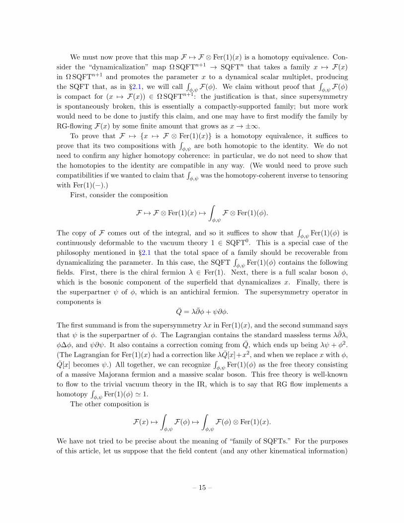
We must now prove that this map F 7→ F ⊗ Fer(1)(x) is a homotopy equivalence. Con-

sider the “dynamicalization” map ΩSQFTn+1 → SQFTn that takes a family x 7→ F(x)

in ΩSQFTn+1 and promotes the parameter x to a dynamical scalar multiplet, producing

the SQFT that, as in §2.1, we will call∫φ,ψ F(φ). We claim without proof that

∫φ,ψ F(φ)

is compact for (x 7→ F(x)) ∈ ΩSQFTn+1: the justification is that, since supersymmetry

is spontaneously broken, this is essentially a compactly-supported family; but more work

would need to be done to justify this claim, and one may have to first modify the family by

RG-flowing F(x) by some finite amount that grows as x→ ±∞.

To prove that F 7→ x 7→ F ⊗ Fer(1)(x) is a homotopy equivalence, it suffices to

prove that its two compositions with∫φ,ψ are both homotopic to the identity. We do not

need to confirm any higher homotopy coherence: in particular, we do not need to show that

the homotopies to the identity are compatible in any way. (We would need to prove such

compatibilities if we wanted to claim that∫φ,ψ was the homotopy-coherent inverse to tensoring

with Fer(1)(−).)

First, consider the composition

F 7→ F ⊗ Fer(1)(x) 7→∫

φ,ψF ⊗ Fer(1)(φ).

The copy of F comes out of the integral, and so it suffices to show that∫φ,ψ Fer(1)(φ) is

continuously deformable to the vacuum theory 1 ∈ SQFT0. This is a special case of the

philosophy mentioned in §2.1 that the total space of a family should be recoverable from

dynamicalizing the parameter. In this case, the SQFT∫φ,ψ Fer(1)(φ) contains the following

fields. First, there is the chiral fermion λ ∈ Fer(1). Next, there is a full scalar boson φ,

which is the bosonic component of the superfield that dynamicalizes x. Finally, there is

the superpartner ψ of φ, which is an antichiral fermion. The supersymmetry operator in

components is

Q = λ∂φ+ ψ∂φ.

The first summand is from the supersymmetry λx in Fer(1)(x), and the second summand says

that ψ is the superpartner of φ. The Lagrangian contains the standard massless terms λ∂λ,

φ∆φ, and ψ∂ψ. It also contains a correction coming from Q, which ends up being λψ + φ2.

(The Lagrangian for Fer(1)(x) had a correction like λQ[x]+x2, and when we replace x with φ,

Q[x] becomes ψ.) All together, we can recognize∫φ,ψ Fer(1)(φ) as the free theory consisting

of a massive Majorana fermion and a massive scalar boson. This free theory is well-known

to flow to the trivial vacuum theory in the IR, which is to say that RG flow implements a

homotopy∫φ,ψ Fer(1)(φ) ≃ 1.

The other composition is

F(x) 7→∫

φ,ψF(φ) 7→

∫

φ,ψF(φ) ⊗ Fer(1)(x).

We have not tried to be precise about the meaning of “family of SQFTs.” For the purposes

of this article, let us suppose that the field content (and any other kinematical information)

– 15 –

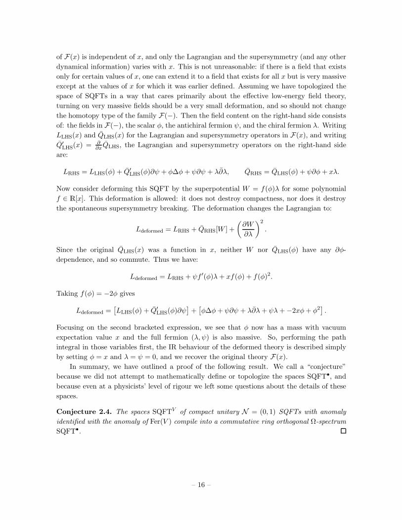
of F(x) is independent of x, and only the Lagrangian and the supersymmetry (and any other

dynamical information) varies with x. This is not unreasonable: if there is a field that exists

only for certain values of x, one can extend it to a field that exists for all x but is very massive

except at the values of x for which it was earlier defined. Assuming we have topologized the

space of SQFTs in a way that cares primarily about the effective low-energy field theory,

turning on very massive fields should be a very small deformation, and so should not change

the homotopy type of the family F(−). Then the field content on the right-hand side consists

of: the fields in F(−), the scalar φ, the antichiral fermion ψ, and the chiral fermion λ. Writing

LLHS(x) and QLHS(x) for the Lagrangian and supersymmetry operators in F(x), and writing

Q′LHS(x) = ∂

∂xQLHS, the Lagrangian and supersymmetry operators on the right-hand side

are:

LRHS = LLHS(φ) + Q′LHS(φ)∂ψ + φ∆φ+ ψ∂ψ + λ∂λ, QRHS = QLHS(φ) + ψ∂φ+ xλ.

Now consider deforming this SQFT by the superpotential W = f(φ)λ for some polynomial

f ∈ R[x]. This deformation is allowed: it does not destroy compactness, nor does it destroy

the spontaneous supersymmetry breaking. The deformation changes the Lagrangian to:

Ldeformed = LRHS + QRHS[W ] +

(∂W

∂λ

)2

.

Since the original QLHS(x) was a function in x, neither W nor QLHS(φ) have any ∂φ-

dependence, and so commute. Thus we have:

Ldeformed = LRHS + ψf ′(φ)λ+ xf(φ) + f(φ)2.

Taking f(φ) = −2φ gives

Ldeformed =[LLHS(φ) + Q′

LHS(φ)∂ψ]+

[φ∆φ+ ψ∂ψ + λ∂λ+ ψλ+−2xφ+ φ2

].

Focusing on the second bracketed expression, we see that φ now has a mass with vacuum

expectation value x and the full fermion (λ, ψ) is also massive. So, performing the path

integral in those variables first, the IR behaviour of the deformed theory is described simply

by setting φ = x and λ = ψ = 0, and we recover the original theory F(x).

In summary, we have outlined a proof of the following result. We call a “conjecture”

because we did not attempt to mathematically define or topologize the spaces SQFT•, and

because even at a physicists’ level of rigour we left some questions about the details of these

spaces.

Conjecture 2.4. The spaces SQFTV of compact unitary N = (0, 1) SQFTs with anomaly

identified with the anomaly of Fer(V ) compile into a commutative ring orthogonal Ω-spectrum

SQFT•.

– 16 –

2.3 Equivariant SQFT• and ’t Hooft anomalies

Let G be a finite group (or a Lie group or . . . , but we will need only the finite group case). The

discussion in the previous section applies equally well if one considers SQFTs, and families

thereof, which are equipped with a nonanomalous G-flavour symmetry. The corresponding

spectrum SQFT•G is a G-equivariant enhancement of the spectrum SQFT•: using it, one can

assign cohomology groups to spaces equipped with G-action. The fundamental reason that

SQFT• admits an equivariant enhancement is that SQFTs admit automorphisms, and so the

collection SQFTn of SQFTs with a given gravitational anomaly is not merely a space, but

rather a groupoid or stack. (The groupoidal/stacky approach to genuinely equivariant spectra

is formalized in [HG07].) If X is any stack, then we can consider the space of maps of stacks

from X to SQFTn, and evaluate its homotopy groups. Taking X = BG the classifying stack

of the group G gives:

SQFT•G = maps(BG,SQFT•),

SQFT•(BG) = SQFT•G(pt) = π0 maps(BG,SQFT•).

We may also consider SQFTs withG-flavour symmetry and prescribed ’t Hooft anomaly ω.

These compile into an orthogonal Ω-spectrum SQFT•G,ω. Because ’t Hooft anomalies add un-

der stacking (i.e. under tensor product of SQFTs), SQFT•G,ω is not a ring spectrum, but it

is a module spectrum for SQFT•G. The algebrotopologists’ name for introducing an ’t Hooft

anomaly ω is twisting : the homotopy groups

SQFT•G,ω(pt) = SQFT•

ω(BG) = π0 SQFT•G,ω

are the “ω-twisted G-equivariant SQFT•-cohomology of a point.”

Where do ’t Hooft anomalies live? For (1+1)-dimensional fermionic QFTs, they live in

the (extended) supercohomology SH3(BG) of the group G [GW14, WG17], which is the 3-layer

spectrum described in §5.4 of [GJF19b] with homotopy groups

SH2(pt) = Z2, SH1(pt) = Z2, SH0(pt) = 0, SH−1(pt) = Z,

and Postnikov k-invariants Sq2 : Z2 → Z2 and Z Sq2 : Z2 → Z, where Sq2 denotes the

second Steenrod squaring operation and Z denotes the integral Bockstein (for the short

exact sequence Z → Z → Z2).

By definition there is a map H•+1(G;Z) → SH•(BG). A long exact sequence shows that

this map is an injection in degree • ≤ 3 (but typically not for larger values of •). It is a

surjection if H•−1(G;Z2) and H•−2(G;Z2) both vanish. In particular, if G is the Schur cover

of simple group, then SH3(BG) = H4(G;Z).

Actually, as emphasized in [GJF19b], it is best to think of SH3(G) instead as the reduced

group cohomology of G with coefficients in the 4-level spectrum fGP×≤4 mentioned in §2.2,

since the basepoint pt → BG gives a canonical isomorphism

(fGP×≤4)

3(BG) = SH3(BG) ⊕ SH3(pt),

– 17 –

and SH3(pt) ∼= Z indexes the gravitational anomaly n = 2(cL − cR). This is consistent

with the general story of twistings of cohomology theories: fGP×≤4 controls all the anoma-

lies, both ’t Hooft and gravitational, for the spectrum SQFT•, and so algebrotopologists

sometimes write the twisted cohomology groups as SQFT•+ωG (−), with •+ ω a total class in

(fGP×≤4)

3(BG).

To build SQFT•G,ω completely correctly, one should rigidify the ’t Hooft anomaly by choos-

ing some representative SQFT Vω with anomaly ω and then asking that points in SQFT•G,ω

have ’t Hooft anomaly identified with the anomaly of Vω. If one just asks that the anomaly

of an SQFT F be equal to ω in cohomology, then there is an ambiguity in this identification

(parameterized by the reduced cohomology group SH2(BG)), analogous to the ambiguity in

promoting an anomalous SQFT with cL = cR to an absolute SQFT. Given that we mod-

elled SQFT• as an orthogonal spectrum, identifying gravitational anomalies with anomalies

of Fer(V ) for real vector spaces V , one might try now to set Vω ?= Fer(V ) for some real

representation V : G → O(n). The anomaly of G acting on Fer(V ) is a characteristic classp12 (V ) ∈ SH3(BG) called the fractional Pontryagin class. (It is in the image of H4(G;Z)

whenever the representation V is Spin.)

Thus one can ask: How many of the classes in SH3(BG) arises as fractional Pontryagin

classes of real representations? This is a supercohomological version of the classical question

of understanding which classes in Hev(G;Z) arise as Chern classes of complex representations.

The answer is: it depends on the group G. To illustrate this, consider the case when G is

a Schur cover of a sporadic group. The calculations in [JFT20, JFT19, JF19] show that

SH3(BG) = H4(G;Z) vanishes if G is one of

M23, 3McL, J4,Ly

and does not vanish but consists entirely of fractional Pontryagin classes for G in

M11, 2M12, 6M22,M24, 2J2,Co3,Co2, 2Co1, 6Suz, 3J3,He.

On the other hand, for the groups G in

2HS,Mon,

it is shown in those papers that SH3(BG) = H4(G;Z) is not generated by fractional Pontrya-

gin classes. The calculations for the other sporadic groups have not been completed.

This might lead the reader to worry that perhaps there is no good representative Vωin general. Fortunately, the main result of [EG18] is that there is, for any finite group G

and anomaly ω ∈ H4(G;Z), a bosonic holomorphic conformal field theory Vω with G-flavour

symmetry and ’t Hooft anomaly ω. The CFT Vω is not canonical, and is of very high central

charge. Although [EG18] focuses on bosonic CFTs, the construction extends to the fermionic

case for any ω ∈ SH3(BG). Any holomorphic conformal field theory can be thought of as an

N = (0, 1) superconformal field theory by simply declaring the supersymmetry operator to

be trivial. Thus we can construct representatives Vω as required.

– 18 –

The two examples from the end of §2.1, Fer(3)⊕24 and V f ⊗ Fer(3), each carry natural

M24-actions. The action on the former permutes the 24 summands, and so (as in the introduc-

tion) we will call it 24⊗Fer(3); we will write “24” for both the standard degree-24 permutation

representation of M24 as well as its enhancement to a TQFT with 24 massive vacua permuted

by M24. The action on the latter is the restriction of the action by Co1 = Aut(V f). Thus

we find classes [24⊗Fer(3)] ∈ SQFT−3ω (BM24) and [V f ⊗Fer(3)] ∈ SQFT−27

ω′ (BM24), where

ω, ω′ are the ’t Hooft anomalies of the various actions. In both cases the action of M24 on

Fer(3) is trivial, and so these classes are the products of classes [24] ∈ SQFT0ω(BM24) and

[V f] ∈ SQFT−24ω′ (BM24) by the class [Fer(3)] ∈ SQFT−3(pt). (The ring SQFT•(pt) acts on

all twisted equivariant cohomologies SQFT•ω(X).) One of the main results of [GJFW21] is

that there is a well-defined class in SQFT−n(pt) for each cobordism class of n-dimensional

manifolds with String structure (and in particular for each class of n-dimensional framed

manifolds), and the 3-sphere S3 = SU(2) with its Lie group framing determines the class

[Fer(3)]. In algebraic topology, generalized cohomology classes determined by S3-with-its-

Lie-group-framing are conventionally named “ν.” Following this convention, we can write

our SCFTs as

[24]ν ∈ SQFT−3ω (BM24), [V f]ν ∈ SQFT−27

ω′ (BM24).

What are the ’t Hooft anomalies ω, ω′? The answer in the former case is complicated, and

so we will do it second. For [V f]ν, the anomaly of M24 is restricted from the anomaly of the

Co1-action on V f. The main result of [JFT20] implies that SH3(Co1) ∼= Z24 is cyclic, gen-

erated by the fractional Pontryagin class p12 of the 24-dimensional projective representation

of Co1. (The paper [JFT20] calculates instead the ordinary cohomology of the Schur cover

Co0 = 2.Co1, but it is not hard to show that the canonical maps SH3(Co1) → SH3(Co0) and

H4(Co0;Z) → SH3(Co0) are both isomorphisms.) Up to a sign convention in the definition of

“’t Hooft anomaly,” p12 is precisely the anomaly of Co1 acting on V f [JF19]. Furthermore,

Theorem 8.1 of [JFT20] asserts that, upon restriction to M24 ⊂ Co1, this anomaly restricts

to −α, where α is the anomaly of Mathieu Moonshine computed in [GPRV13]. Actually,

since different authors might reasonably disagree on the sign of “the anomaly,” it is useful

that [CHVZ18] has compared the multipliers for some elements acting in Mathieu Moonshine

versus in V f (see Table 3 therein). Multipliers depend linearly on the anomaly, and in all

cases checked the anomaly for V f restricts to minus the anomaly from [GPRV13]. Together

with the computer calculation H4(M24;Z) = Z12 from [DSE09] (confirmed using elemen-

tary methods in Theorem 5.1 of [JFT20]), and further calculations from [GPRV13], these

comparisons are enough to establish that

(anomaly of V f)|M24= −(anomaly of Mathieu Moonshine).

But the anomalies of V f and V f have opposite signs. Writing α for the Mathieu Moonshine

anomaly from [GPRV13], we find:

[V f]ν ∈ SQFT−27α (BM24).

– 19 –

Turning to [24]ν ∈ SQFT−3ω (BM24), we must answer the question: What is the ’t Hooft

anomaly of the M24-action on the TQFT 24? The naıve answer, “zero,” misses an important

subtlety, which is that the question is badly posed: ’t Hooft says that there is an anomaly when

a partition function or other datum, which was expected to be G-invariant, in fact changes

by a phase; but in our case those data are often zero because of the vacuum degeneracy.

More precisely, the M24-symmetry on 24 spontaneously breaks to a trivial M23-symmetry.

This trivial M23-symmetry is definitely nonanomalous. But we may consider the total M24-

symmetry to have any anomaly that we choose in the kernel of SH3(M24) = H4(M24;Z) →SH3(M23) = H4(M23;Z). Remarkably, H4(M23;Z) = 0 [Mil00] (that paper in fact shows

that H•(M23;Z) = 0 for • ≤ 5, and provides further information about H•(M23;Z); the

low-cohomology results are confirmed computationally in [DSE09], and the H4 calculation is

confirmed with elementary methods in [JFT20]). Thus we may consider the M24-action on

[24]ν as having any anomaly that we want:

[24]ν ∈ SQFT−27ω (BM24) for any desired ω ∈ SH3(M24) = H4(M24;Z) = Z12.

The same argument can be rephrased algebrotopologically in terms of pushforwards. If

f : H → G is a homomorphism of finite groups, then an SQFT with G-symmetry and

’t Hooft anomaly ω ∈ SH3(BG) determines, by forgetting some information, an SQFT with

H-symmetry and ’t Hooft anomaly f∗ω ∈ SH3(BH). This provides a pullback map

f∗ : SQFT•G,ω → SQFT•

H,f∗ω .

This map has an “adjoint” f∗ : SQFT•H,f∗ω → SQFT•

G,ω. To construct it, note that any map

f : H → G factors canonically as a surjection followed by an injection:

H ։ im(f) → G.

Thus it suffices to describe f∗ when f : H → G is either surjective or injective.

Suppose first that f : H → G is a surjection with kernel K = ker(f). Then f∗ω ∈SH3(BH) restricts trivially to K, and so if F is an SQFT with H-symmetry, the K-action is

nonanomalous and may be gauged. Furthermore, because the anomaly f∗ω of the H-action

is pulled back from G, there is no “mixed anomaly.” It follows that the gauged theory F K

carries a G-action with anomaly ω. The pushforward map f∗ is

f∗ : F 7→ F K.

Note the repeated use of the fact that the anomaly is pulled back from G. If all we knew

was that H acted on F with some anomaly ω′ ∈ SH3(H), and that ω′|K = 0, then there

would be an ambiguity in the meaning of the gauged theory: there would be SH2(K)-many

theories that deserve the name “F K,” parameterized by the SH2(K)-many trivializations

of ω′|K . (Here and throughout, SH• denotes reduced supercohomology.) In our case, we can

choose a canonical gauging because, since f∗ω is restricted from G, it trivializes canonically

– 20 –

on K. Gauging uses up the K-symmetry, but produces a new “magnetic dual” action by

SH1(K) ∼= hom(K,U(1)), and in general the remaining G-action could be extended by this

symmetry (c.f. [BT17] or §2.3 of [JF19]). In our case the extension is trivial because f∗ω

is pulled back from G. If the extension were trivializable but not canonically so, then the

different trivializations might lead to different G-actions with different anomalies. But, again

because f∗ω is pulled back from G, the extension is canonically trivializable, and the resulting

G-action has anomaly ω.

Suppose now that f : H → G is an injection, and let X = G/H denote the space of cosets.

If F is an SQFT with H-symmetry and anomaly f∗ω, then the direct sum (aka disjoint union)

of X-many copies of F can be given a G-action that permutes the copies, and that acts as

H on each copy. Physically, this is an SQFT where the G-symmetry spontaneously breaks to

an H-symmetry. This is the pushforward map.

In both cases, the pushforward f∗ can be described as a type of finite path integral.

Indeed, gauging a K-symmetry is the same as integrating over K-gauge fields, which are

maps from the worldsheet to BK, which is the fibre of BH → BG in the case when H → G

is an injection. When H → G is a surjection, then the fibre of BH → BG is the set X, and

again we are taking an integral over maps to this fibre. This explains the general structure:

f∗ implements a finite path integral over the space of maps from the worldsheet to the fibre

X of the map BH → BG.

As an example, suppose that f : H → G is an inclusion, and ω ∈ SH3(G) is an anomaly

such that f∗ω = 0 ∈ SH3(H). Then we have a pushforward map

f∗ : SQFT•(BH) → SQFT•ω(BG).

The domain is a commutative ring (the codomain is not, if ω 6= 0), with unit 1 ∈ SQFT•(BH)

represented by the trivial “vacuum” SQFT with trivial H-symmetry. The pushforward f∗(1)

is simply the (1+1)-dimensional TQFT with X = G/H many ground states, permuted by

the G-symmetry, and no other structure. (In terms of functorial field theories valued in the

2-category of algebras and bimodules, f∗(1) corresponds to the algebra⊕

X C.) For G = M24

and H = M23, this is the TQFT that we called “24” above. If instead we had chosen

some F ∈ SQFT•(pt), equipped with the trivial H-action (equivalently, pulled back along

BH → pt), then f∗(F) = f∗(1)⊗F = 24⊗F .

For the purposes of explaining Mathieu Moonshine, this looks pretty good. When re-

stricted along pt ⊂ M24, the SQFT 24 ⊗ Fer(3) restricts to Fer(3)⊕24, which we already

saw is nullhomotopic and produces the mock modular form H(τ). If 24 ⊗ Fer(3) were M24-

equivariantly nullhomotopic, then we would produce mock modular forms Hg,h(τ) as desired.

Unfortunately, it is not:

Proposition 2.5. 24 ⊗ Fer(3) is not M24-equivariantly nullhomotopic, for any ’t Hooft

anomaly ω.

Proof. If [24⊗ Fer(3)] = [24]⊗ ν were trivial in SQFT−3ω (BM24), then its restriction to M23

would also be trivial. Since SH3(M23) = 0, this restriction has trivial gauge anomaly, and so

– 21 –

we may gauge the M23-action. If 24⊗Fer(3) were equivariantly nullhomotopic, then so would

be this gauged theory (by gauging the M23-action on the nullhomotopy). In algebrotopological

language, writing f : M23 → M24 and p : M23 → pt, we wish to compute p∗f∗f∗1⊗ ν.

This is purely a TQFT computation. Our goal is to compute the (1+1)-dimensional

TQFT which counts maps from the worldsheet to the quotient stack

24 M23.

But, restricted to M23, 24 splits as 1 ⊔ 23, and so

24 M23 = BM23 ⊔ 23 M23 = BM23 ⊔BM22.

In other words, the TQFT p∗f∗f∗p

∗1 is the direct sum of two TQFTs: pure gauge theory for

M23, and pure gauge theory for M22.

For any finite group G, pure G-gauge theory in (1+1)-dimensions is described by the

group algebra C[G] of G, which is Morita equivalent to the direct sum of #(G/G)-many

copies of C, where #(G/G) means the number of conjugacy classes in G. The group M23 has

17 conjugacy classes, and the group M22 has 12 conjugacy classes. Thus

p∗f∗f∗p

∗1 = 17 + 12 = 29,

and so p∗f∗f∗p

∗1 ⊗ ν = 29ν, represented by the SQFT Fer(3)⊕29. But 29 is not divisible by

24, and so Fer(3)⊕29 is not nullhomotopic by [GJF19a].

One could wonder if perhaps the day would be saved by somehow squeezing in some

discrete torsion, i.e. nontrivial Dijkgraaf–Witten action, into the M22 gauge theory, since

SH2(M22) = H3(M22;Z) = Z6 is nontrivial. This effects a change from the group algebra

C[M22] to a twisted group algebra. The twisted group algebras of M22 are Morita equivalent

to a sum of 10 or 11 copies of C, depending on the twisting, and neither 17 + 10 nor 17 + 11

is divisible by 24.

2.4 Twisted and twined shadows

Proposition 2.5 means that we will not be able to answer Question 1.1 by working just

with the permutation representation of M24. There is another reason to reject it as an

answer. Suppose, contradicting Proposition 2.5, that 24 ⊗ Fer(3) were M24-equivariantly

nullcobordant, and choose a nullcobordism F . For each commuting pair g, h ∈ M24, we may

twist and twine F , thereby producing a partition function ZRR(F)g,h(τ, τ). Following the

logic of Conjecture 2.1, the holomorphic part of ZRR(F)g,h(τ, τ), normalized with a factor of

η(τ), will be a mock modular form (for some subgroup of SL2(Z) depending on g, h) whose

shadow is (the complex conjugate of) the torus one-point function of Q in 24⊗Fer(3), twisted

and twined by g and h.

Since g and h do not act on Fer(3), this shadow factors as

putative shadow = ZRR(24)g,h η(τ)3.

– 22 –

The computation of ZRR(24)g,h is very easy, because 24 itself is very easy, being simply the

TQFT of maps from the worldsheet to the standard permutation representation 24 of M24.

To have a map to this set from a torus twisted and twined by g and h, the value of the map

must be fixed by both g and h, and we discover:

Z(24)g,h ∝ number of common g, h fixed points in 24.

If we were treating 24 as a nonanomalous M24-equivariant TQFT, then the two sides would

be equal. We have written only that they are proportional because of the possibility of a

nontrivial anomaly ω. Indeed, the presence of ω means that the twisted-twined partition

“function” is not really a function at all, but rather a section of a flat line bundle on the

space of spin tori with G-bundles. Under modifying a 3-cocycle representative of ω by dξ, for

some 2-cochain ξ on G, the “function” Z(24)g,h changes by a factor of ξ(g,h)ξ(h,g) .

When g = e is the identity, ZRR(24)e,h is simply the trace of the h-action on 24, which

agrees with the shadows in Mathieu Moonshine (compare [CDH14a]). More generally, if the

subgroup of M24 generated by g and h is cyclic (for example, if g and h have coprime order),

then Z(24)g,h = Z(24)1,x = tr24(x), where x is any generator of the cyclic group. This is

again consistent.

However, if the subgroup generated by g and h is not cyclic, then this putative shadow

is not the shadow of the mock modular form Hg,h(τ) from (generalized) Mathieu Moonshine.

Indeed, [GPRV13] finds that Hg,h(τ) has trivial shadow (i.e. it is holomorphic modular) as

soon as g and h do not generate a cyclic group, and for most such pairs Hg,h simply vanishes.

But there are many rank-2 subgroups of M24 which do have fixed points. A list of all conjugacy

classes of rank-2 abelian subgroups of M24 is available in Table 1 of [GPRV13]. The first entry

on that list, for example, is a Klein-4 subgroup Z22 which acts with 8 fixed points in 24.

Instead, as in Conjecture 1.4, we conjecture that V f ⊗ Fer(3) is nullhomotopic. If

it is, then the twisted and twined partition functions of its nullhomotopy would have, as

their shadows, the functions ZRR(V f)g,h η(τ)3. The antiholomorphicity of V f means that

ZRR(V f)g,h is just an integer: the signed trace of h acting on the ground states of the g-

twisted Ramond sector of V f. When g = 1, these ground states form the Leech lattice

representation Leech ⊗ R of Co0 = 2.Co1. (The double cover comes from the “Gu–Wen

layer” of the anomaly of the Co1-action on V f.) This representation restricts over M24 to

the permutation representation, and so ZRR(V f)1,h = tr24(h) = ZRR(24)1,h, which is the

desired value. More generally, if g, h generate a cyclic group, with cyclic generator x, then

ZRR(V f)g,h = ZRR(V f)1,x = ZRR(24)1,x = ZRR(24)g,h, simply because these two integers

are related by a modular transformation. On the other hand, when g, h generate a rank-2

group, then ZRR(V f)g,h and ZRR(24)g,h may not agree. In fact:

Theorem 2.6. If g, h ∈ M24 generate a rank-2 abelian group, then ZRR(V f)g,h = 0. Thus

Conjecture 1.4 is consistent with the shadows found by [GPRV13].

The calculations of [CdLW19] suggest that there may be an elegant proof of this theorem,

but the author did not find one. Rather, we will prove the theorem by computing all cases.

– 23 –

Proof. The integer ZRR(V f)g,h = ZRR(Vf)g,h depends only on the conjugacy class of the

rank-2 abelian group 〈g, h〉. It transforms with nontrivial multiplier under some congruence

subgroup, and hence must be zero, as soon as the ’t Hooft anomaly restricts nontrivially to

〈h〉, or to any other generator of 〈g, h〉. This leaves only the groups where 〈g, h〉 consists of

elements with M24-conjugacy classes 1, 2A, 3A, 4B, or 6A. (The other nonanomalous elements

in M24 do not participate in rank-2 abelian groups.) In Table 1 of [GPRV13], these are the

entries numbered 1, 2, 3, 17, 18, 19, 25, 26, 28, 29.

In order to study these cases, we must understand the g-twisted Ramond-sectors of V f

for g of M24 conjugacy class 2A, 3A, 4B, and 6A. In fact, the only rank-2 subgroups in

M24 that include a 6A element are generated by a 6A element and a 2A element, and so, by

switching g and h, we do not need to consider the last case.

In order to study these twisted sectors, let us recall a bit about the holomorphic SVOA

V f. It is a lattice SVOA for the D+12 lattice:

D+12 =

λ = (λ1, . . . , λ12) ∈ Z12 ⊔

(Z+ 1

2

)12 such that

∑λi ∈ 2Z

.

It has a canonical translation coset inside R12:

(D+12)R =

λ = (λ1, . . . , λ12) ∈ Z12 ⊔

(Z+ 1

2

)12 such that

∑λi ∈ 2Z+ 1

.

The Ramond sector V fR is built from (D+

12)R in the same way that the Neveu–Schwarz sector

is built from D+12. Namely, V f

R is generated over the Heisenberg algebra Bos(12) by a state Γλfor each λ ∈ (D+

12)R. There is no canonical way to assign a fermion parity operator “(−1)f”

to the R-sector of a holomorphic SVOA, but the relative parity is well-defined, and we will

arbitrarily declare the absolute parity by saying that Γλ is bosonic (resp. fermionic) if λ ∈ Z12

(resp. (Z+ 12)

12).

The N=0 automorphism group (i.e. the automorphism group as an SVOA, ignoring

the supersymmetry) of V f is the Lie group SO+(12), defined as the image of Spin(12) in

the positive half-spin representation. Because of the ’t Hooft anomaly, this group acts only

projectively on the Ramond sector: the group that acts linearly on V fR is Spin(12) itself.

Since SO+(12) is connected, any g ∈ SO+(12) can be conjugated into the maximal torus

T ∼= R12/D+12 ⊂ SO+(12). We will abusively also call this torus element “g,” but we will

write the group law in T additively. Any g ∈ T determines a translated lattice D+12+g ⊂ R12,

from which the g-twisted sector V fg is built. A special case is when g = R is the central

element in SO+(12), in which D+12 + R = (D+

12)R is the canonical translated lattice, and

the notation “V fR ” is consistent. As an element of R12/D+

12, R can be represented by the

vector R = (1, 0, . . . , 0) (mod D+12). More generally, the g-twisted R-sector deserves the name

“V fR+g.” For the symmetries g ∈ M24 ⊂ SO+(12) that we are interested in, the vectors are:

M24 name cycle structure g ∈ T = R12/D+12

2A 1828 (12 ,12 ,

12 ,

12 , 0, 0, 0, 0, 0, 0, 0, 0)

3A 1636 (13 ,13 ,

13 ,

13 ,

13 ,

13 , 0, 0, 0, 0, 0, 0)

4B 142244 (12 ,12 ,

12 ,

14 ,

14 ,

14 ,

14 , 0, 0, 0, 0, 0)

– 24 –

In any sector of any lattice SVOA, L0 acts on the state Γλ with eigenvalue |λ|2/2. If

g preserves a supersymmetry operator Q, then in the g-twisted R-sector the Hamiltonian

L0 − c/24 is a square (of the zero mode of Q, up to a normalization convention) and so takes

only nonnegative values. We are interested in the space of ground states, which are thus in

bijection with those λ ∈ V fR+g with |λ|2 = 1 (since c = 12 for V f). Such a state contributes

a bosonic or fermionic mode according to whether λ− g is integral or half-integral. Each of

the vectors g ∈ T listed above contains at least five 0s. Thus a vector λ ∈ g + (Z + 12)

12

will have at least five entries with absolute value ≥ 12 , and so |λ|2 ≥ 51

4 > 1. It follows

that the g-twisted R-sector has only bosonic ground states. The number of ground states is

then, by modularity, equal to the trace of g acting on the ground states in V fR , which is just

the 24-dimensional representation of M24. This trace tr24(g) is easily read from the above

table: it is the exponent of 1 in the cycle structure. (A priori, there could be both bosonic

and fermionic ground states in the g-twisted R-sector, and only their signed count is equal

to tr24(g).)

For any g acting on any holomorphic conformal field theory V , the g-twisted sectors Vgand VR+g carry projective actions of the centralizer C(g) inside the automorphism group of

V . As we have remarked already, the anomaly for the M24-action on V f is (up to a sign)

the same as the anomaly computed in [GPRV13]. This anomaly determines the projectivity

of the action of C(g) on the g-twisted sectors. (See [GPRV13] for a nice explanation.) The

centralizers C(g) ⊂ M24 of the elements g listed above, and their projective character tables,

are listed in the appendix of [GPRV13].

When g = 2A, we have C(2A) = 24.(23:L3(2)) in the ATLAS notation. Its action on

V fR+2A is genuinely projective. The eight ground states must compile into an 8-dimensional

module. This is the smallest dimension of any projective representation on C(2A). It remains

to identify the correct representation: they are listed under the names χ1, χ2, χ3, χ4 in the

appendix of [GPRV13]. But look at the class called 4A1 therein. It has a nontrivial anomaly,

and so its trace vanishes. Thus we find that the ground states of V fR+2A correspond to the

character χ1. The only nonzero entries in the χ1 correspond to elements h ∈ C(2A) such that

h and g = 2A together generate a cyclic group. This establishes the Theorem for the groups

numbered 1, 2, 3, 17, 18, 19, 28, 29 in Table 1 of [GPRV13].

When g = 3A, we have C(3A) = 3A6, the exceptional Schur cover of the alternating

group A6. The ground states of V fR+3A form a six-dimensional linear representation M ;

because H1(C(3A);U(1)) = 0, there is a canonical trivialization of the projectivity, and so no

phase ambiguities in the actions of elements of C(3A) onM . The centralizer of g inside the full

automorphism group AutN=1(Vf) = Co1 is a group of shape 32.U4(3).2 [CCN+85, Wil83].

This acts through a double cover (32×2).U4(3).2 on V fR+3A, and 6 is the smallest dimension of

any simple representation thereof. The central g ∈ (32 × 2).U4(3).2 acts on all 6-dimensional

representations with trace ±3± 3√−3. It follows that M breaks up over 3A6 as a sum of the

characters labeled χ2, χ3, χ4, χ5, χ8, χ9 in [GPRV13]. For all of these modules, the element

labeled 3A2 acts with trace 0. This establishes the Theorem for the group numbered 33 in

Table 1 of [GPRV13].

– 25 –

Finally, we have the groups 〈g, h〉 numbered 25 and 26, for which g and h are both of

class 4B. According to [GPRV13], C(4B) is a group of shape ((4 × 4):4):2, acting genuinely

projectively on the four ground states of V fR+4B. For both groups (numbers 25 and 26), the

centralizer of 〈g, h〉 has order 16. It follows that h is one of the conjugacy classes named

“4B3,” “4B4,” “4B5,” and “4B7” in the appendix of [GPRV13]. But for h = 4B5 or 4B7, the

group 〈g, h〉 contains an element of class 4A, which has an anomaly (they correspond to the

groups numbered 23 and 24 in Table 1 of [GPRV13]). The classes h = 4B3 and 4B4 act with

trivial trace on all genuinely projective representations of C(4B).

The mock modular forms Hg,h from [GPRV13] are integral in the sense that their co-

efficients, as functions of h, are all virtual characters of projective representations of the

centralizer of g in M24. (Indeed, they are mostly zero.) Thus the equivariant version of the

invariant from [GJF19a] vanishes for V f ⊗ Fer(3): that invariant does not obstruct Conjec-

ture 1.4.

It was observed early in the development of Mathieu Moonshine [GHV12, Gan16] that the

characters that appear (i.e. the coefficients of the q-expansion of H1,h(τ)) are all restrictions

of virtual characters of projective represenations of Co1. However, it is unlikely that the

functions H1,h, let alone Hg,h, have (mock) modular integral extensions to Co1. Said another

way, it is likely that the invariant from [GJF19a] is strong enough to prove:

Conjecture 2.7. V f ⊗ Fer(3) is not Co1-equivariantly nullhomotopic.

2.5 TMF• and tmf•

The main conjecture of [ST04, ST11] (our Conjecture 1.5) is that the spectrum SQFT• is

equivalent to the “universal elliptic cohomology” spectrum TMF• called Topological Modular

Forms. There is quite a lot of evidence in favour of this conjecture, and versions of it were

predicted as early as [Wit87, Wit88, Seg88]. Notably, Witten explained in the first of those

papers that the then-recently-discovered “elliptic genus” of Landweber, Stong, and Ochanine

arises as the Z2-twisted partition function of the N = (1, 1) sigma model (with Z2-action

that breaks the the left-moving supersymmetry), and also introduced what is now known as

the Witten genus by using instead an N = (0, 1) sigma model.

Another piece of evidence supporting Conjecture 1.5 is that the corresponding statement

in (0+1) dimensions is understood [Che06, HST10, Mar10, Ulr19]. Indeed, the construc-

tion from §2.2 with N=1 supersymmetric quantum mechanics models in place of (1+1)-

dimensional QFTs produces a spectrum SQM•. If the SQM models are not required to

support a time-reversal symmetry, then the resulting spectrum SQM• is known to model

the complex K-theory spectrum KU•. If the SQM models are equipped with a time-reversal

symmetry then SQM• models orthogonal K-theory KO•. (The time-reversal symmetry must

satisfy T 2 = +1, corresponding to Pin− under Wick rotation. The Pin+ case T 2 = (−1)f is

not compatible with the dynamicalization procedure leading to a spectrum structure.)

Quantum mechanics has a complete mathematical axiomatization in terms of Hilbert

spaces and von Neumann algebras, and the statement “SQM• = K•” is a mathematical

– 26 –

theorem. Presuming that a complete mathematical axiomatization of unitary, compact (1+1)-

dimensional quantum field theory can be found, Conjecture 1.5 offers an analytic model of

TMF•, for which so far the only known models are homotopy-algebraic. (Progress towards

proving Conjecture 1.5 is available in [Che06, BET18, BET19], which establish versions “over

the Tate curve” and, equivariantly, over C.)

There are in fact three closely-related spectra that go under the name “topological mod-

ular forms,” distinguished by their capitalizations. The first, TMF•, is the space of “weakly

holomorphic topological modular forms”: it is a homotopical refinement of the ring MF• of

integral modular forms that are holomorphic for finite values values of τ , but possibly mero-

morphic at the cusp τ = i∞. (By “integral,” we mean that the q-expansion lives in Z((q)).

Modular forms of weight w are assigned cohomological degree n = −2w.) The algebrotopo-

logical definition of TMF• is a “derived” version of MF•. Specifically, there is a “derived

stack” Mderell which refines the stack Mell of smooth elliptic curves. It carries a “derived

structure sheaf” Oder whose fibre at an elliptic curve E ∈ Mderell is the spectrum presenting

E-elliptic cohomology. The homotopy sheaf π2wOder = L⊗w is the line bundle whose sec-

tions are weight-w modular forms. (Constructing these derived algebrogeometric objects is

hard [GH04, Lur09, Goe10, HM14, Lur18a, Lur18b, Lur19].) Then TMF• is the spectrum of

derived global sections of Oder. This is the spectrum that appears in Conjecture 1.5.

The second spectrum, Tmf•, is the space of “holomorphic topological modular forms,”

analogous to the ring mf• of modular forms that are bounded at τ = i∞. Its definition

parallels TMF• and mf•: compactify Mderell to a derived stack Mder

ell that allows elliptic curves

with nodal singularities, extend the derived structure sheaf, and take derived global sections.

Because of the derived nature of these constructions, the homotopy groups of both TMF• and

Tmf• include information about the cohomology of the line bundles L⊗w. In particular, even

though there are no holomorphic modular forms of negative weight (positive cohomological

degree), the line bundles L⊗w for negative even w do have cohomology over Mell, leading to

nontrivial classes in π−•Tmf = Tmf•(pt) for • > 0.

The physical significance of Tmf• is not yet clear: there probably is an analogue of

Conjecture 1.5 for Tmf•, but a satisfactory one has not yet been proposed. One approach is

suggested in [Mar10], but this author doubts that that method can be made physically sensible

in (1+1) dimensions. A more direct approach would involve a spectral constraint on the

operator L0 in the Ramond sector which is strong enough to assure that the adjusted partition

function Z ′RR(τ) = ZRR(τ)η

2(cR−cL)(τ) converges as τ → i∞. For example, it should rule out

the holomorphic SCFT V f, since that SCFT represents the class 24∆−1 ∈ TMF24(pt),

which is not in the image of Tmf• → TMF•. On the other hand, Tmf21(pt) ∼= Z is generated

by a class that deserves the name 24∆−1ν, which is is in the kernel of Tmf• → TMF•. The

author believes that the generator 24∆−1ν should be represented by the N=(1, 1) SCFT

V f ⊗ Fer(3), but it is not clear how to tune the constraint so as to allow this.

Third, the spectrum tmf• is defined to be the connective cover of Tmf•: as an Ω-spectrum,

tmfn = Tmfn = Ω−nTmf0 for n ≤ 0, but tmfn = BnTmf0 for n > 0. Said another way, tmf•

is built by keeping only the 0-space Tmf0 of the Tmf•-spectrum, which is automatically an

– 27 –

infinite loop space, and then interpreting infinite loop spaces as a special class of spectra. In

homotopy, we have

tmf•(pt) =

Tmf•(pt), • ≤ 0,

0, • > 0.

More generally, if X is a space, then tmf•(X) = Tmf•(X) if • ≤ 0, but not for • > 0. We are

interested in a particular M24-equivariant TMF-class [V f]ν of cohomological degree • = −27.

Nonequivariantly, [V f] = 24∆ ∈ TMF−24(pt) is in the image of Tmf−27(pt), and we

believe that this holds M24-equivariantly as well. Nonequivariantly 24∆ν = 0 ∈ tmf−27(pt),

and hence in TMF−27(pt). Together with Conjecture 1.5, this implies that [V f]ν = 0 ∈SQFT−27(pt).

It is not expected that tmf• itself will admit a natural physical description. The reason

is that any physical description in terms of spaces of SQFTs will naturally lead to a gen-

uinely equivariant enhancement (by working with SQFTs with a given flavour symmetry),

but tmf• is not expected to admit a genuinely equivariant enhancement. A better calcula-

tion than we will attempt in Section 4 would be to work out the equivariant cohomology

Tmf−27α (BM24), and perhaps show, as suggested by Theorem 1.8, that it vanishes away from

the prime p = 2. (Perhaps it even vanishes at p = 2.) But there is no Atiyah–Hirzebruch

spectral sequence for computing equivariant cohomology groups like Tmf−27α (BM24), and so

we will not attempt such a calculation. Rather, in Section 4 we will attempt Tmf−27α (BM24),

approximating the classifying stack BG by its classifying space BG, and the above remarks

identify Tmf−27α (BM24) ∼= tmf−27

α (BM24), since BM24 is just a space, not a stack.

Physically, the difference between BG and BG is the following. As explained in §2.3,

a class in SQFT•ω(BG) is represented by a compact SQFT with G flavour symmetry (and

anomaly ω). A class in SQFT•ω(BG) is instead represented by a family of SQFTs over the

space BG. There is a map SQFT•ω(BG) → SQFT•

ω(BG) which uses the G-action on an

element F ∈ SQFT•ω(BG) to prescribe the monodromies of a family over BG which is locally

constant with value F . This map is definitely not an isomorphism of spaces, because its image

consists of families which are locally constant, whereas a typical family over BG may vary a

lot. But we don’t need it to be, since we care only about homotopy classes. With some work,

a family of SQFTs over BG can be “integrated” to a G-equivariant SQFT, and so one might

expect that SQFT•ω(BG) → SQFT•

ω(BG) is a homotopy equivalence. The problem is that BG

is infinite-dimensional, and so this “integral” will usually fail to produce a compact SQFT. (A

topological space is “finite-dimensional” if it is homotopy equivalent to a finite cell complex.

Except for spaces homotopy equivalent to finite sets, no space is both finite-dimensional

and finite in homotopy.) Indeed, there are sequences of G-equivariant SQFTs which diverge

in SQFT•ω(BG) because their limits are noncompact, but which converge in SQFT•

ω(BG)

because this noncompactness can be concentrated “near infinity” in BG: as you go out along

a cell decomposition of BG, the family stays compact but becomes larger and larger. As such,

one expects SQFT•ω(BG) to be a “completion” of SQFT•

ω(BG), analogous to the famous result

from [AS69] describing KU•(BG) as a completion of KU•(BG). A completion statement for

– 28 –

TMF is known for finite abelian groups G [Lur19]. But we warn that direct computations

in [GM20] show that for G = U(1), the map TMF•(BU(1)) → TMF•(BU(1)) is far from a

completion. (There is a more sophisticated “completion” statement that holds for U(1) at

the level of sheaves over Mell. The failure of TMF•(BU(1)) → TMF•(BU(1)) can then be

traced to the non-affineness of the stack of elliptic curves with U(1)-bundle.)

In addition to the rings MF• and mf• of weakly holomorphic and holomorphic modular

forms, number theorists care also about the ideal cf• ⊂ mf• of cusp forms, which are the

holomorphic modular forms which vanish at τ = i∞. Like modular forms, cusp forms admit

a topological enhancement to a spectrum Tcf• of topological cusp forms. Summarizing a fair

amount of hard work, the idea is to promote the restriction map mf• → O(cusp) = Z to a

map Tmf• → KO•, which was done in [HL16]. Then Tcf• is defined as the homotopy fibre of

Tmf• → KO•. The topology literature seems to contain very little investigation of Tcf•, and,

just like for Tmf•, the physical significance it not yet clear. We will mention one interesting

fact about Tcf•, which makes its behaviour different from the classical case of cf•. Namely, cf•

is the principal ideal inside mf• generated by ∆, and as such it represents (up to suspension,

aka degree-shift) the trivial class in the Picard group of mf•. But ∆ does not lift to an element

in Tmf•(pt), and Tcf• is not isomorphic to a suspension of Tmf•. Rather, in unpublished

work L. Meier has identified the class of Tcf• with the exotic 24-torsion element in the Picard

group of Tmf• called Γ(J ) in [MS16]. (That paper shows that Γ(J ) and suspension together

generate Pic(Tmf•) ∼= Z24 ×Z. Other exotic elements are studied in [HM17, MO20].)

The genus-zero property in Monstrous Moonshine is reformulated in [CDH14b] in terms

of an optimal growth condition which provides the “moonshine” part of Umbral (and in

particular Mathieu) Moonshine. The condition (for M24) is simply that the mock modular

forms Hg,h(τ) grow no worse than q−1/8 as τ → i∞, and are bounded near other cusps.

Recall from §2.1 our proposal that Hg,h(τ) is the holomorphic part of η(τ)ZRR(F)g,h(τ, τ),

for some SQFT F with with cylindrical ends ∂F = V f ⊗ Fer(3) of cohomological degree

n = −28, whereas the homotopy theory convention for Witten genera is to work with the

adjusted partition function Z ′RR(τ, τ ) = ZRR(τ, τ )η(τ)

−n. The optimal growth condition then

becomes the statement that the adjusted function Hg,h(τ)η(τ)27 = O(q1), i.e. it is a “mock

cusp form.” This leads us to propose the following answer to Question 1.3:

Conjecture 2.8. The M24-equivariant class [V f]ν, refining the cusp form 24∆ν = 0 ∈Tmf−27(pt), is M24-equivariantly nullhomotopic in the spectrum Tcf• of topological cusp

forms.

3 Ordinary cohomology of M24

In order to run the Atiyah–Hirzebruch spectral sequence for tmf•ω(BM24)[12 ], we will need

good control over the ordinary group cohomology rings H•(M24;Z[12 ]) and H•(M24;F3). We

find it necessary to invert the prime 2 simply because the 2-local computations are too hard.

These rings were computed in [Tho94, Gre96]. We will review and extend that analysis: our

goal is to have explicit control over the action of the first Steenrod cube P on H•(M24;F3).

– 29 –

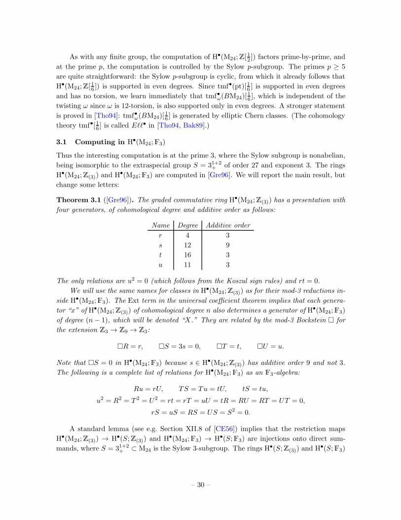
As with any finite group, the computation of H•(M24;Z[12 ]) factors prime-by-prime, and

at the prime p, the computation is controlled by the Sylow p-subgroup. The primes p ≥ 5

are quite straightforward: the Sylow p-subgroup is cyclic, from which it already follows that

H•(M24;Z[16 ]) is supported in even degrees. Since tmf•(pt)[16 ] is supported in even degrees

and has no torsion, we learn immediately that tmf•ω(BM24)[16 ], which is independent of the

twisting ω since ω is 12-torsion, is also supported only in even degrees. A stronger statement

is proved in [Tho94]: tmf•ω(BM24)[16 ] is generated by elliptic Chern classes. (The cohomology

theory tmf•[16 ] is called Eℓℓ• in [Tho94, Bak89].)

3.1 Computing in H•(M24;F3)

Thus the interesting computation is at the prime 3, where the Sylow subgroup is nonabelian,

being isomorphic to the extraspecial group S = 31+2+ of order 27 and exponent 3. The rings

H•(M24;Z(3)) and H•(M24;F3) are computed in [Gre96]. We will report the main result, but

change some letters:

Theorem 3.1 ([Gre96]). The graded commutative ring H•(M24;Z(3)) has a presentation with

four generators, of cohomological degree and additive order as follows:

Name Degree Additive order

r 4 3

s 12 9

t 16 3

u 11 3

The only relations are u2 = 0 (which follows from the Koszul sign rules) and rt = 0.

We will use the same names for classes in H•(M24;Z(3)) as for their mod-3 reductions in-

side H•(M24;F3). The Ext term in the universal coefficient theorem implies that each genera-

tor “x” of H•(M24;Z(3)) of cohomological degree n also determines a generator of H•(M24;F3)

of degree (n− 1), which will be denoted “X.” They are related by the mod-3 Bockstein for

the extension Z3 → Z9 → Z3:

R = r, S = 3s = 0, T = t, U = u.

Note that S = 0 in H•(M24;F3) because s ∈ H•(M24;Z(3)) has additive order 9 and not 3.

The following is a complete list of relations for H•(M24;F3) as an F3-algebra:

Ru = rU, TS = Tu = tU, tS = tu,

u2 = R2 = T 2 = U2 = rt = rT = uU = tR = RU = RT = UT = 0,

rS = uS = RS = US = S2 = 0.

A standard lemma (see e.g. Section XII.8 of [CE56]) implies that the restriction maps

H•(M24;Z(3)) → H•(S;Z(3)) and H•(M24;F3) → H•(S;F3) are injections onto direct sum-

mands, where S = 31+2+ ⊂ M24 is the Sylow 3-subgroup. The rings H•(S;Z(3)) and H•(S;F3)

– 30 –

are computed in [Lew68, Lea91, Lea92]. In particular, the third of those articles confirms

the following result due to [MT95] (the order of final publication did not match the order in

which the preprints were originally circulated):

Proposition 3.2 ([MT95]). Let A1, A2, A3, A4 denote the four maximal abelian subgroups

of S = 31+2+ , each isomorphic to Z3 ×Z3. The total restriction map

H•(S;F3) →∏

i

H•(Ai;F3)

is an injection.

Since H•(M24;F3) ⊂ H•(S;F3), it follows in particular that we can compute inside

H•(M24;F3) by computing restrictions to subgroups isomorphic to Z3 × Z3. Let us de-

scribe these subgroups. First, M24 has two conjugacy classes of elements of order 3. Class 3A

consists of those elements in M24 that act in the degree-24 permutation representation with

cycle structure 1633; class 3B acts with cycle structure 38. The central Z3 ⊂ S consists of 3A-

elements. There are also two conjugacy classes of subgroups Z3×Z3 ⊂ M24. Both subgroups

are maximal-abelian. One of them, which we will call simply Z3A ×Z3A, consists entirely of

3A-elements. The other is Z3A × Z3B. In addition to the identity element, it contains two

3A-elements (forming a Z3-subgroup), and the other six elements are of class 3B. The “Weyl

groups” W (A) = N(A)/A of these maximal abelian subgroups of M24 are as large as possible

given the conjugacy classes of elements:

W (Z3A×Z3A) =N(Z3A×Z3A)

Z3A×Z3A

∼= GL2(F3), W (Z3A×Z3B) =N(Z3A×Z3B)

Z3A×Z3B

∼= D12.

By D12 we mean the dihedral group of order 12, isomorphic to the upper Borel(∗ ∗0 ∗

)⊂

GL2(F3). These and other claims about M24 are easily checked in the computer algebra

program GAP [GAP].

For any finite group and any abelian subgroup A ⊂ G and for any ring R, the restriction

map H•(G;R) → H•(A;R) lands within the Weyl-invariant subring H0(W (A); H•(A;R)). We

therefore conclude:

H•(M24;F3) ⊂ H0(GL2(F3); H•(Z3A ×Z3A;F3))×H0(D12; H

•(Z3A ×Z3B;F3)).

The next step is to understand the right-hand side. Let us choose “coordinates” on Z3A×Z3A

and Z3A ×Z3B, writing Y , resp. Z, for the homomorphisms onto the “fibre” Z3A, resp. and

onto the “base” Z3A or Z3B. After identifying Z3 = F3, these coordinates give classes in

H1(Z3 ×Z3;F3). The full algebra H•(Z3 ×Z3;F3) is then a graded polynomial algebra

H•(Z3 ×Z3;F3) = F3[Y,Z, y, z]

where y = Y and z = Z are in degree 2, and the only relations are the ones imposed by

the Koszul sign rules: Y 2 = Z2 = Y Z + ZY = 0. Note also that mod-3 reduction identifies

– 31 –

H•(Z3 × Z3;Z) with ker ⊂ H•(Z3 × Z3;F3) (except in degree 0), and that this ring is

generated by y and z and the degree-3 element w = yZ − Y z = (Y Z). In particular, the

subring of H•(Z3 ×Z3;F3) consisting of even-degree elements with integral lifts is F3[y, z].

The D12-action on F3[Y,Z, y, z] is generated by the following three automorphisms:

(Y,Z, y, z) 7→ (−Y, z,−y, z), (Y,Z, y, z) 7→ (Y,−z, y,−z),(Y,Z, y, z) 7→ (Y + Z,Z, y + z, z).

To generate the full GL2(F3)-action, it suffices to include also the automorphism

(Y,Z, y, z) 7→ (Z, Y, z, y).

Lemma 3.3. The subring of F3[y, z] invariant under (y, z) 7→ (y + z, z) is F3[z, c] where

c = y(y + z)(y − z) = y3 − yz2 is of cohomological degree 6. The subring of F3[y, z, w] is

F3[z, w, c].

Note that F3[y, z, w] = H•(Z3 ×Z3;Z) except in degree 0.

Proof. Certainly z, c, and w are invariant. Suppose p(y, z) = p0zn + p1yz

n−1 + · · · + pnyn

is an invariant homogeneous polynomial of polynomial degree n (cohomological degree 2n).

Then the largest i with pi 6= 0 must be divisible by 3. Indeed, otherwise under y 7→ y + z,

the coefficient on yi−1zn−i+1 will change by ipi 6= 0. So the space of invariant degree-n

polynomials is at most (1 + ⌊n3 ⌋)-dimensional. But this is the dimension of the space of

degree-n polynomials in F3[z, c]. The second claim follows from the first together with the

fact that F3[y, z, w] = F3[y, z]⊕ wF3[y, z], since w2 = 0 by the Koszul sign rules.

We note also that z and c are not invariant under y ↔ z, but that z6 + c2 = y6 + y4z2 +

y2z4 + z6 and z2c2 = y6z2 + y4z4 + y2z6 are.

We can now work out the restrictions to Z3A × Z3A and Z3A × Z3B of the integral

generators r, s, t, u. First, r has cohomological degree 4. There are no GL2(F3)-invariant

degree-4 classes, and so r|Z3A×Z3A= 0. Then Proposition 3.2 implies that r|Z3A×Z3B

6= 0,

and so is proportional to z2, as that is the only degree-4 class invariant under y 7→ y + z.

Changing the sign of r if necessary, we learn:

r|Z3A×Z3A= 0, r|Z3A×Z3B

= z2.

The extension class R is also immediate, since it is an invariant degree-3 class satisfying

R = r.

R|Z3A×Z3A= 0, R|Z3A×Z3B

= Zz.

Note that w is a degree-3 class invariant under z 7→ y+ z and in the kernel of , but it picks

up a sign under some of the D12 transformations, and so cannot appear here.

The next classes worth considering are the generators T, t, since rT = rt = 0. Thus

both of these classes restrict trivially to Z3A × Z3B, since z2 is not a zero-divisor. Thus

– 32 –

T and t restrict nontrivially to Z3A × Z3A by Proposition 3.2. Since t is an integral class

of cohomological degree 16, its restriction to Z3A × Z3A must a polynomial in y and z of

polynomial degree 8 invariant under all of GL2(F3). By using Lemma 3.3, it is easy to see

that the only such polynomial is c2z2 = y6z2+y4z4+y2z6. Changing the sign of t as necessary,

we have:

t|Z3A×Z3A= y6z2 + y4z4 + y2z6, t|Z3A×Z3B

= 0.

As for T |Z3A×Z3A, we need a GL2(F3)-invariant degree-15 class satisfying T = t. One could

worry that there could be multiple choices. By Lemma 3.3, the only degree-15 class in the

kernel of which is GL2(F3)-invariant up to a sign is w(c2 + z6), but this class changes sign

under some of the involutions in GL2(F3). So T is uniquely determined by invariance and

T = t. We have:

T |Z3A×Z3A= Y (yz6 − y3z4) + Z(y6z − y4z3), T |Z3A×Z3B

= 0.

We next consider the degree-12 generator s. It must have nontrivial restrictions to both

Z3A × Z3A and Z3A × Z3B, since neither rs nor st vanishes. The restriction to Z3A × Z3A

is a polynomial in y and z of degree 6, invariant under all of GL2(F3), and so must be

c2 + z6 = y6 + y4z2 + y2z4 + z6, after possibly changing the sign of s. The restriction to

Z3A × Z3B is some linear combination of c2 and z6. But note that, upon further restriction

to the fibre Z3A, the two restrictions must agree. On the other hand, we have the freedom

to change s 7→ s ± r3 without changing the presentation of H•(M24;Z) in Theorem 3.1. We

will choose the modification so that s|Z3B= 0. Thus we may assume:

s|Z3A×Z3A= y6 + y4z2 + y2z4 + z6, s|Z3A×Z3B

= y6 + y4z2 + y2z4.

We will consider the two degree-11 generators S and u at the same time. It will be

convenient to replace u with v = u − S. Note that S = v = 0, and so the restrictions of

both must land in F3[y, z, w], where as above w = (Y Z) = yZ − Y z. Theorem 3.1 provides

rS = 0 and tv = 0. Therefore S|Z3A×Z3B= 0 and v|Z3A×Z3A

= 0. By Lemma 3.3, the other

restrictions are of the form wp(z, c), where the polynomial p(z, c) is of homogeneous degree

4 in y and z. After tracking the behaviour under z 7→ −z and y 7→ −y, the only option is

p(z, c) = zc = y3z − yz3, and so:

S|Z3A×Z3A= Y (yz4 − y3z2) + Z(y4z − y2z3), S|Z3A×Z3B

= 0.

The signs of S and u are not independent if we want to preserve the relation tS = tu from

Theorem 3.1, and the author was not able to identify the correct sign for the restriction of

v = u− S. We do have:

v|Z3A×Z3B= 0, v|Z3A×Z3B

= ±(Y (yz4 − y3z2) + Z(y4z − y2z3)

).

Last, we have the degree-10 generator U , which must satisfy U = u = v + S. Since U

is of even degree and not in the kernel of , its restriction must be of the form p(y, z)Y Z, for

– 33 –

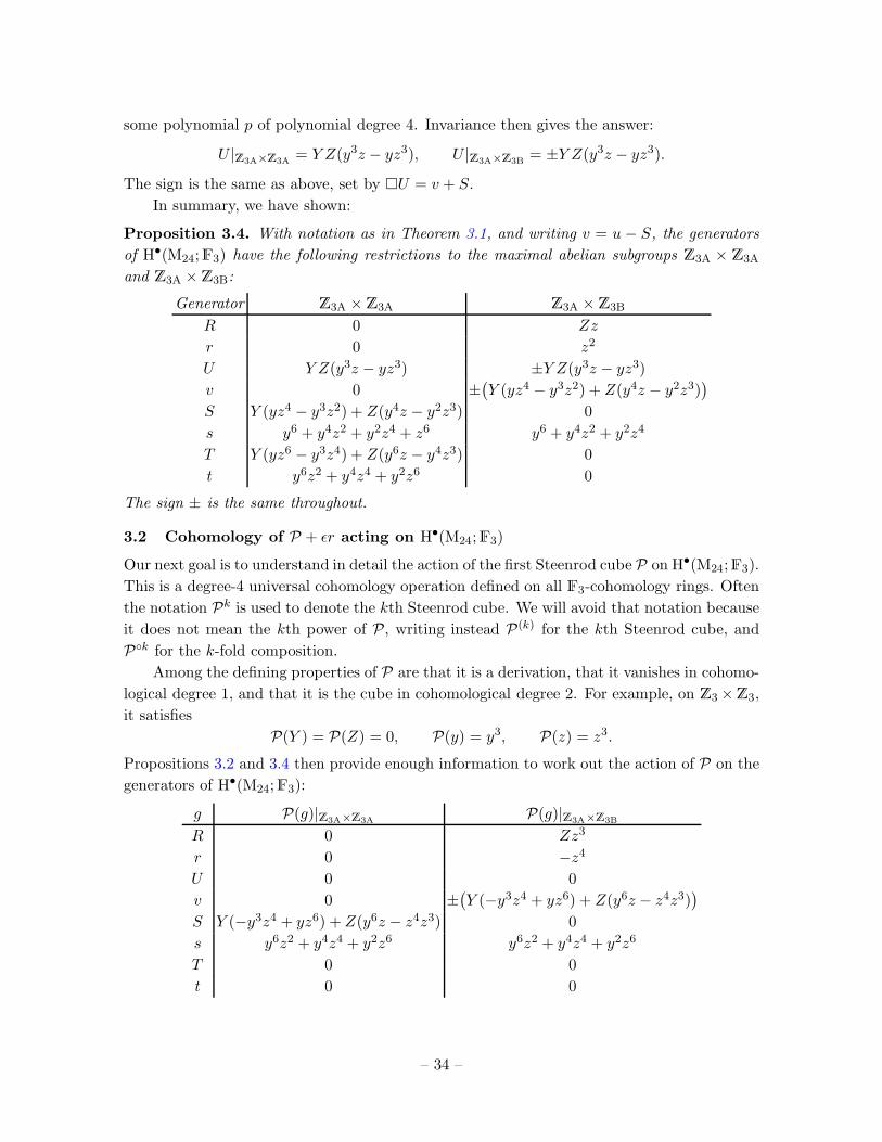
some polynomial p of polynomial degree 4. Invariance then gives the answer:

U |Z3A×Z3A= Y Z(y3z − yz3), U |Z3A×Z3B

= ±Y Z(y3z − yz3).

The sign is the same as above, set by U = v + S.

In summary, we have shown:

Proposition 3.4. With notation as in Theorem 3.1, and writing v = u− S, the generators

of H•(M24;F3) have the following restrictions to the maximal abelian subgroups Z3A × Z3A

and Z3A ×Z3B:

Generator Z3A ×Z3A Z3A ×Z3B

R 0 Zz

r 0 z2

U Y Z(y3z − yz3) ±Y Z(y3z − yz3)

v 0 ±(Y (yz4 − y3z2) + Z(y4z − y2z3)

)

S Y (yz4 − y3z2) + Z(y4z − y2z3) 0

s y6 + y4z2 + y2z4 + z6 y6 + y4z2 + y2z4

T Y (yz6 − y3z4) + Z(y6z − y4z3) 0

t y6z2 + y4z4 + y2z6 0

The sign ± is the same throughout.

3.2 Cohomology of P + ǫr acting on H•(M24;F3)

Our next goal is to understand in detail the action of the first Steenrod cube P on H•(M24;F3).

This is a degree-4 universal cohomology operation defined on all F3-cohomology rings. Often

the notation Pk is used to denote the kth Steenrod cube. We will avoid that notation because

it does not mean the kth power of P, writing instead P(k) for the kth Steenrod cube, and

Pk for the k-fold composition.

Among the defining properties of P are that it is a derivation, that it vanishes in cohomo-

logical degree 1, and that it is the cube in cohomological degree 2. For example, on Z3 ×Z3,

it satisfies

P(Y ) = P(Z) = 0, P(y) = y3, P(z) = z3.

Propositions 3.2 and 3.4 then provide enough information to work out the action of P on the

generators of H•(M24;F3):

g P(g)|Z3A×Z3AP(g)|Z3A×Z3B

R 0 Zz3

r 0 −z4U 0 0

v 0 ±(Y (−y3z4 + yz6) + Z(y6z − z4z3)

)

S Y (−y3z4 + yz6) + Z(y6z − z4z3) 0

s y6z2 + y4z4 + y2z6 y6z2 + y4z4 + y2z6

T 0 0

t 0 0

– 34 –

From this we learn:

Proposition 3.5. With notation as in Proposition 3.4, the first Steenrod cube P acts as:

P(R) = Rr, P(U) = 0, P(S) = T, P(T ) = 0,

P(r) = −r2, P(v) = vr ±Rs, P(s) = sr + t, P(t) = 0.

Recalling that u = v + S, we note that

P(u) = vr ±Rs+ T = (u− S)r ±Rs+ T = ur + T ±Rs,

since Sr = 0.

Proof. The most interesting case is P(v); the other cases are left to the reader. Recall that

v, and hence P(v), vanishes when restricted to Z3A ×Z3A. Their other restrictions are

v|Z3A×Z3B= ±

(Y (yz4 − y3z2) + Z(y4z − y2z3)

),

P(v)|Z3A×Z3B= ±

(Y (yz6 − y3z4) + Z(y6z − y4z3)

),

where for example we use P(yz4−y3z2) = y3z4+4yz6−3y5z2−2y3z4 = yz6−y3z4. Comparing

P(v)|Z3A×Z3Bwith vr|Z3A×Z3B

= vz2, we find a discrepency:

(P(v) − vr)|Z3A×Z3B= ±Z

((y6z − y4z3)− z2(y4z − y2z3)

)= ±Z(y6z + z4z3 + y2z5).

Factoring out Zz = R|Z3A×Z3Bgives ±s|Z3A×Z3B

.

Fix some ǫ ∈ F3. The specific understanding that we seek is the following: we will

calculate the “cohomology” of the D = P+ ǫr. This operator is not a differential in the usual

sense: D D 6= 0. Rather, it is a 3-differential in the sense that its cube is zero:

Lemma 3.6. Let X be a space, and choose x ∈ H4(X;F3). Then the operator D = P +x on

H•(X;F3) satisfies D3 = 0.

Proof. Expanding (P + x)3, we have:

D3 = P3 + P2 x+ P x P + x P2 + P x2 + x P x+ x2 P + x3.

The Adem relations provide P3 = 0 and P2 = −P(2), where P(2) denotes the second

Steenrod power. The statement “P is a derivation” may be summarized as:

P x = xP + P(x).

Here and in the sequel, by “xP” we mean of course x P, i.e. apply P and then multiply

by x, whereas “P(x)” means multiplication by P(x). Thus we find:

D3 = 0 + (P2(x) + 2P(x)P + xP2) + (P(x)P + xP2) + xP2

+ (2xP(x) + x2P) + (xP(x) + x2P) + x2P + x3.

– 35 –

Since we are in characteristic 3, everything cancels to

D3 = P2(x) + x3.

But P2(x) = −P(2)(x) = −x3 since x has degree 4.

Appendix A contains an extended discussion of 3- and higher differentials. For our

purposes, it suffices to record the following. A usual differential on a K-vector space makes it

into a module for the algebra K[D]/(D2); the usual cohomology is the result of decomposing

the module as a direct sum of indecomposables, and discarding the free summands. We have

instead an action of F3[D]/(D3) on a vector space V , and its cohomology H∗(V,D) is the result

of decomposing V as a sum of indecomposable F3[D]/(D3)-modules and discarding the free

summands. Whereas in the usual case the non-free indecomposable module is unique, over

F3[D]/(D3) there are two isomorphism classes of non-free indecomposable modules, of F3-

dimensions 1 and 2. So H∗(V,D) is not just a vector space, but rather picks up a Z2-grading in

addition to any cohomological grading on V . One of the punchlines of Appendix A is that this

Z2-grading is really a fermionic grading: H∗ converts the two-dimensional indecomposable

F3[D]/(D3)-module into an odd line F0|13 . The other punchline is that H∗ is functorial and

symmetric monoidal.

To illustrate this, and as a warm-up to the M24-case that we care about, let us study

the cohomology of P + ǫa2 on H•(Z3;F3) = F3[A, a], where A has degree 1 and a = A has

degree 2. Since P(A) = 0, multiplication by A is an isomorphism of 3-complexes between

the even-degree cohomology F3[a] and the odd-degree cohomology AF3[a]. So it suffices to

understand the cohomology of D = a3 ∂∂a + ǫa2 on F3[a], where ǫ ∈ F3. On monomials, we

have D(ai) = (i+ ǫ)ai+2. For ǫ = 0, this complex looks like:

a0

a1

a2

a3

a4

a5

a6

a7

a8

a9

a10

a11

· · ·

· · ·+1

−1 +1

−1 +1

−1 +1

−1

The non-free summands—the cohomology—are a0 and a1 → a3. For ǫ = 1, we have

instead:

a0

a1

a2

a3

a4

a5

a6

a7

a8

a9

a10

a11

· · ·

· · ·

+1

−1 +1

−1 +1

−1 +1

−1

The cohomology is just a0 → a2. Finally, for ǫ = −1, we see:

a0

a1

a2

a3

a4

a5

a6

a7

a8

a9

a10

a11

· · ·

· · ·

−1 +1

−1 +1

−1 +1

−1 +1

– 36 –

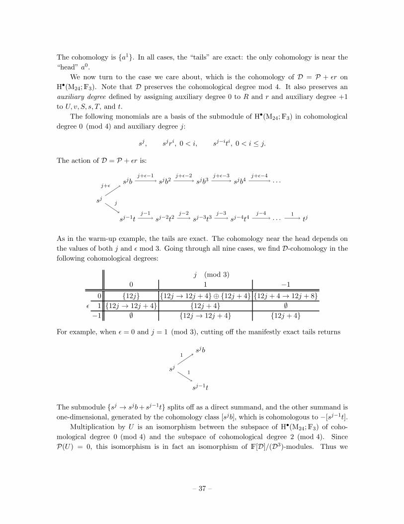
The cohomology is a1. In all cases, the “tails” are exact: the only cohomology is near the

“head” a0.

We now turn to the case we care about, which is the cohomology of D = P + ǫr on

H•(M24;F3). Note that D preserves the cohomological degree mod 4. It also preserves an

auxiliary degree defined by assigning auxiliary degree 0 to R and r and auxiliary degree +1

to U, v, S, s, T, and t.

The following monomials are a basis of the submodule of H•(M24;F3) in cohomological

degree 0 (mod 4) and auxiliary degree j:

sj, sjri, 0 < i, sj−iti, 0 < i ≤ j.

The action of D = P + ǫr is:

sj

sjb sjb2 sjb3 sjb4 · · ·

sj−1t sj−2t2 sj−3t3 sj−4t4 · · · tj

j+ǫ

j+ǫ−1 j+ǫ−2 j+ǫ−3 j+ǫ−4

j

j−1 j−2 j−3 j−4 1

As in the warm-up example, the tails are exact. The cohomology near the head depends on

the values of both j and ǫ mod 3. Going through all nine cases, we find D-cohomology in the

following cohomological degrees:

j (mod 3)

0 1 −1

ǫ

0 12j 12j → 12j + 4 ⊕ 12j + 4 12j + 4 → 12j + 81 12j → 12j + 4 12j + 4 ∅

−1 ∅ 12j → 12j + 4 12j + 4

For example, when ǫ = 0 and j = 1 (mod 3), cutting off the manifestly exact tails returns

sj

sjb

sj−1t

1

1

The submodule sj → sjb+ sj−1t splits off as a direct summand, and the other summand is

one-dimensional, generated by the cohomology class [sjb], which is cohomologous to −[sj−1t].

Multiplication by U is an isomorphism between the subspace of H•(M24;F3) of coho-

mological degree 0 (mod 4) and the subspace of cohomological degree 2 (mod 4). Since

P(U) = 0, this isomorphism is in fact an isomorphism of F[D]/(D3)-modules. Thus we

– 37 –

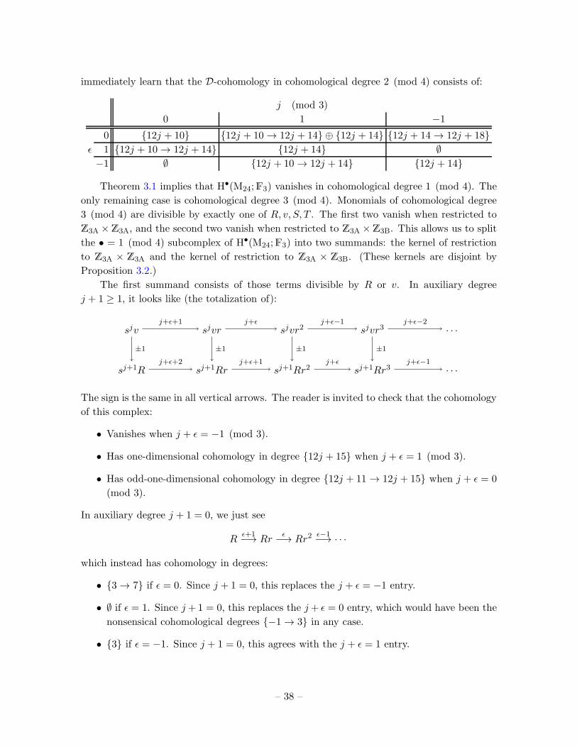
immediately learn that the D-cohomology in cohomological degree 2 (mod 4) consists of:

j (mod 3)

0 1 −1

ǫ

0 12j + 10 12j + 10 → 12j + 14 ⊕ 12j + 14 12j + 14 → 12j + 181 12j + 10 → 12j + 14 12j + 14 ∅

−1 ∅ 12j + 10 → 12j + 14 12j + 14

Theorem 3.1 implies that H•(M24;F3) vanishes in cohomological degree 1 (mod 4). The

only remaining case is cohomological degree 3 (mod 4). Monomials of cohomological degree

3 (mod 4) are divisible by exactly one of R, v, S, T . The first two vanish when restricted to

Z3A ×Z3A, and the second two vanish when restricted to Z3A ×Z3B. This allows us to split

the • = 1 (mod 4) subcomplex of H•(M24;F3) into two summands: the kernel of restriction

to Z3A × Z3A and the kernel of restriction to Z3A × Z3B. (These kernels are disjoint by

Proposition 3.2.)

The first summand consists of those terms divisible by R or v. In auxiliary degree

j + 1 ≥ 1, it looks like (the totalization of):

sjv sjvr sjvr2 sjvr3 · · ·

sj+1R sj+1Rr sj+1Rr2 sj+1Rr3 · · ·

±1 ±1 ±1 ±1

j+ǫ+1 j+ǫ j+ǫ−1 j+ǫ−2

j+ǫ+2 j+ǫ+1 j+ǫ j+ǫ−1

The sign is the same in all vertical arrows. The reader is invited to check that the cohomology

of this complex:

• Vanishes when j + ǫ = −1 (mod 3).

• Has one-dimensional cohomology in degree 12j + 15 when j + ǫ = 1 (mod 3).

• Has odd-one-dimensional cohomology in degree 12j + 11 → 12j + 15 when j + ǫ = 0

(mod 3).

In auxiliary degree j + 1 = 0, we just see

Rǫ+1−→ Rr

ǫ−→ Rr2ǫ−1−→ · · ·

which instead has cohomology in degrees:

• 3 → 7 if ǫ = 0. Since j + 1 = 0, this replaces the j + ǫ = −1 entry.

• ∅ if ǫ = 1. Since j +1 = 0, this replaces the j + ǫ = 0 entry, which would have been the

nonsensical cohomological degrees −1 → 3 in any case.

• 3 if ǫ = −1. Since j + 1 = 0, this agrees with the j + ǫ = 1 entry.

– 38 –

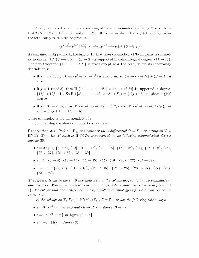
Finally, we have the summand consisting of those monomials divisible by S or T . Note

that P(S) = T and P(T ) = 0, and Sr = Tr = 0. So, in auxiliary degree j +1, we may factor

the total complex as a tensor product:

sj j−→ sj−1tj−1−→ · · · 2−→ stj−1 1−→ tj ⊗ S +1−→ T

As explained in Appendix A, the functor H∗ that takes cohomology of 3-complexes is symmet-

ric monoidal. H∗(S +1−→ T) = S → T is supported in cohomological degrees 11 → 15.The first tensorand sj → · · · → tj is exact except near the head, where its cohomology

depends on j:

• If j = 2 (mod 3), then sj → · · · → tj is exact, and so sj → · · · → tj ⊗ S → T is

exact.

• If j = 1 (mod 3), then H∗(sj → · · · → tj) = sj → sj−1t is supported in degrees

12j → 12j + 4. So H∗(sj → · · · → tj ⊗ S → T) = 12j + 15 in cohomological

degree.

• If j = 0 (mod 3), then H∗(sj → · · · → tj) = 12j and H∗(sj → · · · → tj ⊗ S →T) = 12j + 11 → 12j + 15.

These cohomologies are independent of ǫ.

Summarizing the above computations, we have:

Proposition 3.7. Pick ǫ ∈ F3, and consider the 3-differential D = P + ǫr acting on V =

H•(M24;F3). Its cohomology H∗(V,D) is supported in the following cohomological degrees

modulo 36:

• ǫ = 0 : 0, 2 → 6, 10, 11 → 15, 11 → 15, 12 → 16, 16, 22 → 26, 26,27, 27, 28 → 32, 35 → 39.

• ǫ = 1 : 0 → 4, 10 → 14, 11 → 15, 15, 16, 26, 27, 35 → 39.

• ǫ = −1 : 2, 3, 11 → 15, 12 → 16, 22 → 26, 23 → 27, 27, 28,35 → 39.

The repeated terms in the ǫ = 0 line indicate that the cohomology contains two summands in

those degrees. When ǫ = 0, there is also one nonperiodic cohomology class in degree 3 →7. Except for that one non-periodic class, all other cohomology is periodic with periodicity

element s3.

On the subalgebra F3[R, r] ⊂ H•(M24;F3), D = P + ǫr has the following cohomology:

• ǫ = 0 : r0 in degree 0 and R→ Rr in degree 3 → 7.

• ǫ = 1 : r0 → r1 in degree 0 → 4.

• ǫ = −1 : R in degree 3.

– 39 –

4 The Atiyah–Hirzebruch spectral sequence for tmf•ω(BM24)

With the ordinary 3-local cohomology of BM24 understood, we are now ready to analyze the

3-local structure of tmf•ω(BM24). We will do so by analyzing its Atiyah–Hirzebruch spectral

sequence.

4.1 General comments about AHSSs

Any space X and spectrum E• determine an Atiyah–Hirzebruch spectral sequence. (The name

refers to [AH61] but the proof there consists essentially of a reference to [CE56], and [Ada74]

attributes the construction to unpublished work of Whitehead. Further important early devel-

opments are in [Mau63].) Spectral sequences are an algebrotopolical version of perturbation

theory. As with any perturbative calculation, the goal is to approximate some nonperturba-

tive object. In the AHSS case, that nonperturbative object is E•(X), the E•-cohomology of

the space X.

The rough idea of the AHSS is the following. Imagine that X is a CW complex and

that you have fixed some cochain model for E•. Then a cochain for En(X) assigns, to each

m-cell in X, an element of En−m. The cohomology En(X) is the cohomology for some total

differential on this set of cochains. The AHSS perturbatively approximates that total differ-

ential. The 0th approximation entirely ignores the topology of X: for a cell x ∈ X and a

cochain x 7→ e(x), the 0th approximation is (d0e)(x) = dE(e(x)), where dE is the differential

in (the cochain model for) E•. The 1st approximation includes some attaching information

for the cells in X. By definition, the Ek-page of a spectral sequence is the cohomology of the

(k − 1)th approximation of the total differential. It is always bigraded by the dimension m

of a cell in X and the E-degree n of a cochain. In the AHSS case, the E2 page is

Em,n2 = Hm(X; En(pt)).

As one “turns the page,” one includes higher-order corrections, which take into account how

the homotopy groups E•(pt) are connected. The result is an infinite sequence of finer and

finer approximations to E•(X).

Any time one works perturbatively, one must worry about two related problems:

• Does the perturbative expansion converge at all?

• Does the perturbative expansion converge to the object one wishes to compute?

In particular, perhaps there are “nonperturbative effects” not seen in the perturbative ex-

pansion, so that it does not in fact calculate the desired result.

In the case of AHSSs, this second problem is present as soon as one tries to extend

from spaces to stacks. Indeed, suppose X is a stack with classifying space X. Then there

is an AHSS which tries to approximate E•(X), with E2 page H•(X; E•(pt)). But ordinary

cohomology does not distinguish stacks from spaces: H•(X; E•(pt)) = H•(X; E•(pt)). The

– 40 –

higher differentials also do not distinguish X from X. As a result, this AHSS will at best

converge to E•(X), which in general is not isomorphic to E•(X) (compare §2.5).

Most textbooks confirm convergence of AHSSs in only very limited circumstances: when

the E•(pt) is bounded below, or when H•(X;Z) is bounded above. More general convergence

results are available in [Boa99]. In particular, Theorem 12.4 of that paper says that the

AHSS for E•(X) does indeed converges “conditionally” to E•(X), for any spectrum E and

space X. (The convergence is in the “colimit” topology. We will not here discuss the different

topologies in which the convergence might hold.) Theorem 7.1 of that paper gives conditions

under which this “conditional” convergence is in fact “strong,” which is what one wants for

applications. In particular, as explained in the remark following Theorem 7.1 of that paper,

for a conditionally convergent spectral sequence to converge strongly, it suffices if each entry

Em,n supports only finitely many nonzero differentials, i.e. if there are only finitely many k

for which dk : Em,nk → Em+k,n−k+1

k is nonzero. In particular, we find:

Lemma 4.1. Suppose E is a spectrum all of whose homotopy groups E•(pt) are finitely

generated as abelian groups, and suppose that X = BG is the classifying space of a finite

group. Then the AHSS H•(BG; E•(pt)) ⇒ E•(BG) converges strongly.

Proof. Since G is finite and En(pt) is finitely generated, Em,n2 = Hm(BG;En(pt)) is finite if

m > 0. It therefore can support only finitely many differentials.

And, other than d0 and d1, the m = 0 column supports no differentials at all! Indeed, the

d2 and higher differentials in an AHSS are always stable cohomology operations, and stable

cohomology operations always vanish in degree m = 0.

The proof of Lemma 4.1 does not automatically apply for cohomology with twisted coef-

ficients, because the differentials in the twisted case can involve multiplication and higher

Massey products with the twisting parameter. (The m > 0 part of the proof still ap-

plies.) The K-theory case is explored in detail in [AS06], where all higher differentials

are computed: for twisting parameter α ∈ H3(X;Z), the d2k differentials in the AHSS

H•(X; KU(pt)) ⇒ KU•α(pt) vanish, and the d2k+1 differential is a stable operation plus a

k-fold Massey product with α. But Massey products (other than the ordinary product) van-

ish in degree m = 0, and so again the m = 0 column supports only finitely many (namely,

one) differential, and the AHSS converges strongly.

The overall message of [Boa99] is that one should run spectral sequences without worrying

too much about convergence, and then check convergence at the end. This is because, for

a conditionally convergent spectral sequence, strong convergence is simply a property of the

sequence itself. Following this advice, we will compute the first few differentials in the AHSS

for tmf•ω(BM24). This will be enough for us to confirm in Corollary 4.8 that the AHSS

converges.

4.2 Review of tmf•(pt)[12 ]

The first step towards constructing the AHSS H•(M24; tmf•(pt)[12 ]) ⇒ tmf•ω(BM24)[12 ] is to

understand the coefficient ring tmf•(pt)[12 ]. An excellent reference for looking up information

– 41 –

about this ring is the chapter [Hen14] of [DFHH14], and [Mat12] provides a nice survey of

how the computations are done.

Write cw for the weight-w Eisenstein series, normalized so that cw(q) = 1+O(q). Recall

that the ring mf of integral SL(2,Z)-modular forms, which are “holomorphic” in the sense of

being bounded at the cusp τ = i∞, is

mf = Z[c4, c6,∆]/(c34 − c26 − 1728∆).

In particular, after inverting 6, we have mf[16 ] = Z[16 ][c4, c6]. As in §2.5, we will think of mf as a

cohomologically-graded ring mf•, with the modular forms of weight w in cohomological degree

−2w. (Our insistence of working with cohomological gradings means that mf• is supported

in nonpositive degrees.) Justifying the names, there is a ring map tmf•(pt) → mf•. It is an

isomorphism away from 6:

tmf•(pt)[16 ]∼→ mf•[16 ] = Z[16 ][c4, c6].

It follows that the map tmf•(pt) → mf• has kernel exactly the torsion in tmf•(pt). It is

traditional to name non-torsion classes in tmf•(pt) by their images in mf•.

(So far as the author knows, there is no interesting spectrum E• with homotopy groups

E•(pt) = mf•: the only such spectrum is a product of Eilenberg–Mac Lane spaces, and

represents H•(−;mf•). The map on coefficients tmf•(pt) → mf• does not lift to a spectrum

map tmf• → H•(−;mf•).)

We will keep 2 inverted, and describe tmf•(pt)[12 ] in terms of its map to mf•[12 ]. This

map is almost a surjection. In particular, its image contains the Eisenstein series c4, c6, and

hence powers of 27∆ = 164 (c

34 − c62). (At the prime 2, c4 is in the image of tmf•(pt), but c6 is

not: only 2c6 is.) In fact, m∆k is in the image of tmf•(pt)[12 ] if and only if mk = 0 (mod 3):

tmf•(pt)[12 ] contains nontorsion classes 3∆, 3∆2, and ∆3. The curly brackets remind

that 3∆ is not divisible by 3 in tmf•(pt)[12 ].

The kernel of the map tmf•(pt)[12 ] → mf•[12 ], i.e. the torsion in tmf•(pt)[12 ], is periodic of

cohomological degree 72, with periodicity element ∆3. All torsion in tmf•(pt)[12 ] has additive

order 3. A framed compact manifold of dimension n determines a class [M ] ∈ tmf−n(pt).

In the case of a group manifold for a connected simply connected compact group G, the

corresponding class is represented, assuming Conjecture 1.5, by the antiholomorphic SCFT

consisting of n = dimG antichiral free Majorana–Weyl fermions, with supersymmetry en-

coding the bracket on the Lie algebra of G [GJFW21]. In the introduction, we mentioned

already the class ν represented by the 3-sphere SU(2). Note that [Hen14] calls this class “α”

in the section describing the 3-local structure of tmf•(pt) (and “ν” in the section describing

the 2-local structure). Another important class is represented by the 10-dimensional group

manifold Spin(5). For want of a better name, we will call this class “µ”; it is called “β”

in [Hen14]. These classes satisfy ν2 = µ2ν = µ5 = 0 in tmf•(pt)[12 ]. Furthermore, there

is a nontrivial Massey product 〈ν, ν, ν〉 = −2µ = µ, which the reader is invited to think

through geometrically by decomposing Spin(5) into two pieces. (Hint: use the inclusion

– 42 –

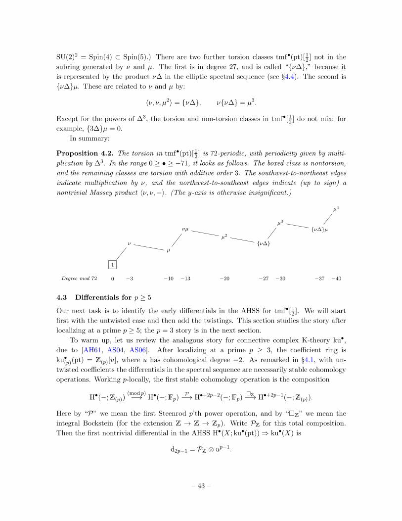
SU(2)2 = Spin(4) ⊂ Spin(5).) There are two further torsion classes tmf•(pt)[12 ] not in the

subring generated by ν and µ. The first is in degree 27, and is called “ν∆,” because it

is represented by the product ν∆ in the elliptic spectral sequence (see §4.4). The second is

ν∆µ. These are related to ν and µ by:

〈ν, ν, µ2〉 = ν∆, νν∆ = µ3.

Except for the powers of ∆3, the torsion and non-torsion classes in tmf•[12 ] do not mix: for

example, 3∆µ = 0.

In summary:

Proposition 4.2. The torsion in tmf•(pt)[12 ] is 72-periodic, with periodicity given by multi-

plication by ∆3. In the range 0 ≥ • ≥ −71, it looks as follows. The boxed class is nontorsion,

and the remaining classes are torsion with additive order 3. The southwest-to-northeast edges

indicate multiplication by ν, and the northwest-to-southeast edges indicate (up to sign) a

nontrivial Massey product 〈ν, ν,−〉. (The y-axis is otherwise insignificant.)

Degree mod 72 −3 −10 −13 −20 −27 −30 −37 −400

1

µ

µ2

µ3

µ4

ν

νµ

ν∆

ν∆µ

4.3 Differentials for p ≥ 5

Our next task is to identify the early differentials in the AHSS for tmf•[12 ]. We will start

first with the untwisted case and then add the twistings. This section studies the story after

localizing at a prime p ≥ 5; the p = 3 story is in the next section.

To warm up, let us review the analogous story for connective complex K-theory ku•,

due to [AH61, AS04, AS06]. After localizing at a prime p ≥ 3, the coefficient ring is

ku•(p)(pt) = Z(p)[u], where u has cohomological degree −2. As remarked in §4.1, with un-

twisted coefficients the differentials in the spectral sequence are necessarily stable cohomology

operations. Working p-locally, the first stable cohomology operation is the composition

H•(−;Z(p))(mod p)−→ H•(−;Fp)

P−→ H•+2p−2(−;Fp)Z−→ H•+2p−1(−;Z(p)).

Here by “P” we mean the first Steenrod p’th power operation, and by “Z” we mean the

integral Bockstein (for the extension Z → Z → Zp). Write PZ for this total composition.

Then the first nontrivial differential in the AHSS H•(X; ku•(pt)) ⇒ ku•(X) is

d2p−1 = PZ ⊗ up−1.

– 43 –

In the formula, we have identified the E2 page as H•(X; ku•(pt)(p)) ∼= H•(X;Z(p))⊗Z(p)[u2],

and “up−1” means multiplication thereby. In fact, the same formula works also at the prime

p = 2, with P replaced by Sq2, so that PZ is the integral lift of Sq3. This gives the d3differential identified in [AH61]. The higher differentials are similar, with P replaced by

higher Steenrod pth powers.

To see that d2p−1 is in fact a differential, note that (mod p) Z = p is the mod-p

Bockstein (for the extension Zp → Zp2 → Zp), and so:

PZ PZ = Z P p P (mod p).

But an Adem relation says

P p P = P(2) p +p P(2),

where P(2) denotes the second Steenrod power, and p (mod p) and Z p both vanish.

The occurrence of P(2) here is related to the occurrence of P(2) in the next differential d4p−3.

The twisted story is only slightly more complicated. As explained in [AS04, AS06], the

K-theory of a space X can be twisted by any class ω ∈ H3(X;Z) (and more generally, at the

prime 2, by classes in the supercohomology SH• of [GW14, WG17]). The twisting modifies

the d3 differential to

d3 = d3 − ω ⊗ u.

Higher differentials are also modified, now by Massey products with ω. For example,

d5 = d5 − 〈ω, ω,−〉 ⊗ u2.

Note that the Massey product 〈ω, ω,−〉 is not well-defined on the E2-page of the AHSS, but

it is well-defined on the E4 page.

With the K-theory case understood, we can describe the tmf story. This is simplest if

we work locally at a prime p ≥ 5. There is a map of spectra H : tmf• → ku•JqK, which on

homotopy groups takes a nontorsion class in tmf•(pt) to its q-expansion (with the power of

u just recording the weight of the corresponding modular form). The name “H” is because

of its physical interpretation as the map SQFT• → KU•((q)) that sends an SQFT to its

Hilbert space, with the parameter q encoding the S1-action that rotates the spatial circle.

The existence of H forces the values of some differentials in the AHSS for tmf•, since the

construction of AHSSs depends functorially on the spectrum. Indeed, suppose we are working

p-locally, so that the E2 page is H•(X;Z(p))[c4, c6]. As earlier, just because differentials are

stable and because tmf•(pt)(p) has no torsion, the first possible nonzero differential is d2p−1.

Suppose that ξ ∈ H•(X;Z(p))[c4, c6] is some class. If

d2p−1(Hξ) = (PZ ⊗ up−1)(Hξ)

is not zero in ku•(X)(p)JqK, then certainly d2p−1(ξ) must also be nonzero. Indeed, we find

that, in the AHSS for tmf•:

d2p−1 = PZ ⊗A

– 44 –

for some modular form A of weight p − 1 which maps to up−1 via H. Actually, that’s not

quite the requirement: if H(A) = up−1, then the q-expansion of A is 1 ∈ Z(p)JqK, which

does not happen for a modular form of nonzero weight. The trick is that PZ factors through

mod-p reduction, and so its image consists just of p-torsion classes. Thus we do not need

H(A) = up−1 on the nose, but only that H(A) ≡ up−1 (mod p). Said another way, the

q-expansion of A should be 1 ∈ FpJqK.

Working over Fp, there is only one weight-(p− 1) modular form with trivial q-expansion,

namely the Hasse invariant. When p ≥ 5, it is liftable to an integral modular form. The

standard lift is the weight-(p − 1) Eisenstein series cp−1, and so we could set:

d2p−1 = PZ ⊗ cp−1.

But we don’t in fact need to choose a lift: different lifts differ by multiples of p, whereas the

image of PZ is p-torsion, so different lifts give the same d2p−1 differential. Indeed, all we need

is a criterion for checking liftability. Sufficient conditions are:

Lemma 4.3. A mod-p modular form of weight w admits an integral lift if H1(Mell;L⊗w) has

no p-torsion, where Mell is the compactified moduli stack of elliptic curves, and L⊗w is the

line bundle whose sections are weight-w modular forms.

Proof. This is automatic from the cohomology long exact sequence

. . .p−→ H0(Mell;L

⊗k)mod p−→ H0(Mell;L

⊗k/p)Z−→ H1(Mell;L

⊗k)p−→ . . . .

But the only torsion in H•(Mell;L⊗k) is at the primes 2 and 3. Thus, for p ≥ 5, in fact

all mod-p modular forms admit integral lifts.

4.4 Differentials when p = 3

If we try to repeat the p ≥ 5 story at the prime p = 3, we run into the following issue.

Suppose f ∈ tmf•(pt) is nontorsion, and that x ∈ H•(X;Z(3)). Then the E2 page of the

AHSS contains the class x⊗ f . The map H sends this class to the class x⊗H(f) on the E2

page of the AHSS for ku•(X)(3)JqK, which supports a d5 differential sending it to

x⊗H(f) 7→ ZP(x)⊗ u2H(f),

where P now denotes the first Steenrod cube, and we will leave out from the notation the

mod-3 reduction. As above, this suggests that x ⊗ f should support a d5 differential of the

form

d5 : x⊗ f?7→ ZP(x) ⊗ (integral lift of Af),

where A denotes the mod-3 Hasse invariant.

By Lemma 4.3, the obstruction to lifting Af is measured by the class Z(Af) = αf ∈H1(Mell;L

⊗k)(3), where α = Z(A). This cohomology group turns out to vanish except when

k = 2 + 12j, in which case it is a Z3 generated by α∆j. We therefore find that the above d5differential is well-defined if f is a multiple of 3, c4, c6, or their translates by powers of ∆.

– 45 –

Modulo this ideal, the nontorision subring is just F3[∆3], and our d5 differential is not

defined on classes of the form x ⊗ ∆3j . Conveniently, it doesn’t need to be. The presence

of ν ∈ tmf−3(pt) means that the tmf•-AHSS may contain a d4-differential equal (up to an

irrelevant sign) to

d4 = P ⊗ ν.

Indeed, the fact that the map from the sphere spectrum to tmf• is an equivalence in low

degrees forces the existence of such a differential. (The sphere spectrum is initial among E∞

ring spectra. This implies that, for the sphere spectrum, any differential which is allowed to

be nonzero is in fact nonzero.) The d5 differential needs only to be defined on the cohomology

of d4, and if ZP(x) 6= 0 so that “d5(x⊗∆3j) = ZP(x)⊗ (lift of A∆3j)” is undefined, then

d4(x⊗∆3j) = (−1)deg xP(x)⊗ ν∆3j 6= 0.

The sign comes from the Koszul sign rules, since ν has odd degree.

These d4 and d5 differentials are closely related. Indeed, the class α = Z(A) represents

the class ν in the following sense. There is a elliptic spectral sequence converging to tmf•(pt)(3)whose E2 page is H•(Mell;L

⊗•)(3). In this spectral sequence, α is a permanent cocycle, and

its image on the E∞ page is the associated graded element to ν.

Returning to the d5 differential, we must work out d5(x ⊗ f) whenever f ∈ tmf•(pt)

satisfies νf = 0. The discussion above about lifts of multiplication by the Hasse invariant

implies:

d5(x⊗ c4) = ZP(x) ⊗ c6,

d5(x⊗ c6) = ZP(x) ⊗ c24,

d5(x⊗ 3∆) = 0.

These almost completely determine the behaviour of d5, since it must be linear for the action

by tmf•(pt), and so, if f1, f2 ∈ tmf•(pt) with νf1 = 0, then

d5(x⊗ f1f2) = d5(x⊗ f1)f2.

Note that this is consistent with the above rules because ZP(x) is 3-torsion. Indeed, for

f = c4c6, we would a priori face a discrepancy like

d5(x⊗ c4)c6 − d5(x⊗ c6)c4 = ZP(x)⊗ (c26 − c34) = ZP(x)⊗ 5763∆,

but this vanishes since 576 is divisible by 3.

These rules do not quite determine the behaviour of d5 on the whole E5 page: there is

the possibility of a differential of the form

d5(x⊗ µ2) = ZP(x) ⊗ f

– 46 –

for some f ∈ tmf−24(pt) = Span(3∆, c34). Because ZP(x) is always 3-torsion, this map

only depends on the class of f modulo 3. Furthermore, f must be in the kernel of H :

tmf−24(pt)/3 → ku−24JqK/3 = F3JqK. So the only possibility is, up to sign,

d5 : x⊗ µ2?7→ ZP(x) ⊗ 3∆.

One hint that there is in fact such a differential comes from the elliptic spectral sequence.

The class µ2 ∈ tmf•(pt) is represented on the E2 page by a class β2 ∈ H4(Mell;L⊗12)(3).

Although νµ2 = 0 in tmf•(pt), αβ2 6= 0 in H5(Mell;L⊗14)(3); it is instead the image of a

d5-differential emitted by ∆. Rather than exploring the elliptic spectral sequence in more

detail, we will give an alternate proof:

Proposition 4.4. The AHSS for tmf• includes a nontrivial d5 differential supported by

classes of the form x⊗ µ2.

Proof. Our strategy is to compare our AHSS with the computations from [Hil07], which

computes the 3-local tmf•-homology of the symmetric group S3. More specifically, that

paper computes the 3-local homology tmf•(ΣBS3)(3), where BS3 is the classifying space of

S3, and ΣBS3 is its suspension. We will focus on the specific value

tmf29(ΣBS3) = 0.

Since [Hil07] computes homology, not cohomology, in this proof only we will work with

homological, rather than cohomological, gradings. The homology and cohomology of a point

are related by

tmf•(pt) = tmf−•(pt).

But note that the same formula does not hold with pt replaced by other spaces.

The AHSS for homology reads:

Hm(ΣBS3; tmfn(pt)) ⇒ tmfm+n(ΣBS3).

Homology AHSSs converges strongly by Theorem 12.2 of [Boa99]. The differentials in homol-

ogy AHSSs are essentially the same as the differentials in cohomology AHSSs, because in both

cases they come form the Postnikov tower of the coefficient spectrum. The only difference is

to understand the cohomology operations instead as homology operations. This is easy: the

groups H•(X;F3) and H•(X;F3) are dual, and so one uses the dual map.

We have the following Z(3)- and F3-homology of ΣBS3:

H•(ΣBS3;Z(3)) =

Z, • = 0,

F3tk, • = 4k, k > 0,

0, else,

H•(ΣBS3;F3) =

F3tk, • = 4k,

F3Tk, • = 4k + 1, k > 0,

0, else,

– 47 –

These are easily seen by noting that S3 = C3 ⋊C2. We have named basis vectors tk, Tk, with

tk denoting both the integral class and its mod-3 reduction. The Bockstein is (Tk) = tk,

and the first Steenrod power is

P(tk) = (k − 1)tk−1, P(Tk) = kTk−1.

In total degree 29, the only nonzero entries on the E2 page are:

t4 ⊗ νµ ∈ H16(ΣBS3; tmf13(pt)), T2 ⊗ µ2 ∈ H9(ΣBS3; tmf13(pt)).

The former is the image of a d4 differential:

d4(t5 ⊗ µ) = P(t5)⊗ νµ = t4 ⊗ νµ.

The latter class must also be killed by some differential in order to confirm the compu-

tation tmf29(ΣBS3) = 0 from [Hil07]. It is not the image of a differential. Indeed, the only

classes of total degree 30 on the E2 page that could emit differentials to T2 ⊗ µ2 are t5 ⊗ µ,

which we already saw does not survive d4, and

T5 ⊗ νµ = d4(T6 ⊗ µ),

and so also does not survive d4. Thus T2 ⊗ µ2 must emit a differential. But the only degree

possible is d5, and so we conclude

d5(T2 ⊗ µ2) 6= 0.

And so general AHSSs for tmf include a d5 differential supported by classes of the form

x⊗ µ2.

After d4,d5, the next differential allowed by general considerations about degrees of stable

operations is d8. To derive its formula, compare with the analysis in [AS06]: d8 arises as the

“reason” that d4 d4 = 0. What is this reason? The vanishing of

d24 = P2 ⊗ ν2

has nothing to do with the “X” part of the differential, because P2 6= 0. Rather, it vanishes

because ν2 = 0 in cohomology. This means that the d8 differential will include a Massey

product. Indeed, suppose that x ⊗ f ∈ ker(d4) simply because νf = 0, while perhaps

P(x) 6= 0. Then, if we imagine working at cochain level, we instead have

d4(x⊗ f) = (−1)deg xP(x)⊗ d1(F ),

where d1 is the differential computing tmf•(pt) and F is some cochain for which d1(F ) = νf .

Imagine a “total differential” d1 + d4. One can find cochain formulas so that d1 and d4commute, but (d1 + d4)

2 will not vanish. Rather, (d1 + d4)2 = d24, which at cochain level is

d24(x⊗ f) = P2(x)⊗ νd1(F ) = −P2(x)⊗ d1(νF ).

– 48 –

To correct this, we include a d8 differential whose commutator with d1 is x⊗ f 7→ −P2(x)⊗d1(νF ). I.e. we should have

d8(x⊗ f)?= −P2(x)⊗ (νF +Nf),

where N is some cochain such that d1(N) = ν2. This is an okay thing to write because

d1(νF +Nf) = −νd1(F ) + d1(N)f = −ν2f + ν2f = 0 at cochain level.

The combination νF +Nf is, by definition, the Massey product 〈ν, ν, f〉. We find:

d8 = −P2 ⊗ 〈ν, ν,−〉.

We emphasize that this is only well-defined on the d4-cohomology. Indeed, 〈ν, ν, f〉 doesn’t

exist unless νf = 0. Furthermore, the class F is defined only modulo cocycles, but if you

change F by a cocycle, then you change 〈ν, ν, f〉 by a multiple of ν, and so do not change d8 on

the d4-cohomology. There is no essential ambiguity in the choice of N because tmf−7(pt) = 0.

In the AHSS for some generic 3-local E∞ ring spectrum E , there is room for one further term

in the d8 differential, equal to −P2 ⊗ λ for some λ ∈ E−7(pt). But again we use that

tmf−7(pt) = 0 to rule out that possibility here.

Although we will not need it, we mention that an analysis as in the p ≥ 5 case identifies a

d9-differential of the form P(2)⊗ (integral lift of A2). Note that, although the Hasse invariant

A itself does not have an integral lift, A2 lifts to c4. Finally, if we twist by an ’t Hooft

anomaly ω ∈ H4(X;Z(3)), the only difference is that the Steenrod operator P is replaced by

the operator D = P − ω. All together, we find:

Proposition 4.5. The AHSS H•(X; tmf•(pt)) ⇒ tmf•ω(X)(3) includes the following differ-

entials, with D = P − ω:

• There is a d4 differential of the form

d4 = D ⊗ ν.

• The multiples of classes c4, c6, and µ2 support a d5 differential of the form

d5 = ZD ⊗

fc4 7→ fc6,

fc6 7→ fc24,

fµ2 7→ f3∆.

• There is a d8 differential of the form

d8 = −D2 ⊗ 〈ν, ν,−〉.

• There is a d9 differential of the form

d9 = −ZD2 ⊗ c4.

There are also higher differentials which we will not work out.

– 49 –

4.5 Running the spectral sequence

We are now ready to understand the AHSS H•(BM24; tmf•(pt)[12 ]) ⇒ tmf•ω(BM24)[12 ], where

ω ∈ H4(M24;Z[12 ]) = F3r, with r as in Section 3. Given Conjecture 1.4, we are interested in

the value of tmf•ω(BM24)[12 ] for • ≡ 1 (mod 4), and specifically • = −27.

As observed in [Tho94], at the primes p ≥ 5 the E2 page is H•(BM24;Z(p))[c4, c6], where

the ring H•(BM24;Z(p)) vanishes if p 6∈ 5, 7, 11, 13, and for p ∈ 5, 7, 11, 13 it is a polyno-

mial ring in a generator xp of cohomological degree 2(p − 1) and additive order p. Thus all

differentials vanish for degree reasons, and the spectral sequence stabilizes on the E2 page.

The differentials do play a role, however: they lead to extensions. Indeed, let xp = xpcp−1,

which is of total degree 0 on the E∞ page. Then, by the q-expansion map H to K-theory, we

see that the translates of xpFp[xp] on the E∞-page compile to copies of the p-adic integers

Z(p) in tmf•(BM24)(p). For the purposes of this paper, all that we care about is that, for

p ≥ 5, tmf•(BM24)(p) is supported in degrees • ≡ 0 (mod 4).

We put aside the prime p = 2 for being too complicated, leaving only the prime p = 3. The

first few differentials for the AHSS H•(BM24; tmf•(pt)) ⇒ tmf•ω(BM24)(3) are summarized in

Proposition 4.5. A typical term on the E2 page has shape x ⊗ f , where f ∈ tmf•(pt) and

x ∈ H•(M24;Z(3)) if f is nontorsion and x ∈ H•(M24;F3) if f is torsion. With some caveats,

the differentials sort into two sets. If f is nontorsion (and not a power of ∆3), then x ⊗ f

only supports d5 and d9 differentials. If f is torsion (and not a translate of µ2) then x ⊗ f

only supports d4 and d8 differentials.

By Theorem 3.1, H•(M24;Z(3)) is supported only in degrees • ≡ 3, 4 (mod 4). Therefore

the E2-page entries x ⊗ f with f nontorsion are also only in degrees • ≡ 3, 4 (mod 4). We

remark that the differentials here are nontrivial, because Proposition 3.5 implies:

ZP(u) = Z(ur + T ±Rs) = t± rs 6= 0.

But, since we care mostly about the case • ≡ 1 (mod 4), these differentials don’t affect us.

Therefore we may focus on classes of the form x⊗ f with

f ∈ 1, ν, µ, νµ, µ2, ν∆, µ3, ν∆µ, µ4

or the translates thereof by powers of ∆3. Except for µ2, these classes only support d4 and d8differentials. Since d5(x ⊗ µ2) is an integral class times 3∆, it has degree 3 or 4 (mod 4),

and so does not interact with the • ≡ 1 (mod 4) case. Thus for the purposes of computing

tmf•ω(BM24)[12 ] for • ≡ 1 (mod 4), we may work just with the subring of the E2 page of the

form

H•(M24;F3)⊗ F31, ν, µ, νµ, µ2, ν∆, µ3, ν∆µ, µ4,and just with the differentials

d4 = D ⊗ ν, d8 = −D2 ⊗ 〈ν, ν,−〉,

where D = P − ω.

– 50 –

Recall from Proposition 4.2 the action of the maps ν and 〈ν, ν,−〉. Writing H =

H•(M24;F3), we therefore find ourselves interested in the following total complex:

H1D−→ Hν

D2

−→ HµD−→ Hνµ

D2

−→ Hµ2D2

−→ Hν∆ D−→ Hµ3D2

−→ Hν∆µ D−→ Hµ4

This is an ordinary cochain complex because D is a 3-differential by Lemma 3.6. Its cohomol-

ogy is closely related to the cohomology of D itself, which is listed in Proposition 3.7. Indeed,

both ker(D)/ im(D2) and ker(D2)/ im(D) vanish whenever D is exact. More generally, both

ker(D)/ im(D2) and ker(D2)/ im(D) are of the same total dimension as the cohomology of

D (with both ∗ and cohomology ∗ → ∗ thought of as 1-dimensional; this is the total

dimension of the super-vector-space-valued cohomology from Appendix A). The precise co-

homological degrees of cohomology classes depends on whether we use ker(D)/ im(D2) or

ker(D2)/ im(D), but their degrees mod 4 do not depend, since D preserves the cohomological

degree mod 4.

The cohomology of the above total complex at the entries H1, Hµ2, and Hµ4 is more

complicated, but for our purposes irrelevant. Indeed, 1, µ2, and µ4 have cohomological

degrees • ≡ 0 (mod 4), and, by Theorem 3.1, H vanishes in degrees • ≡ 1 (mod 4). Thus

the cohomologies at those entries also vanish in degrees • ≡ 1 (mod 4). Combining all of our

calculations, we find the following:

Theorem 4.6. Let ω = −ǫr with ǫ ∈ F3 and notation for H•(M24;Z(3)) as in Theorem 3.1.

On the E9 page of the AHSS H•(BM24; tmf•(pt)[12 ]) ⇒ tmf•ω(BM24)[12 ], the cohomology in

total degree • ≡ 1 (mod 4) is the following. Write Υ = U ⊗ µ, and note that Υ2 = 0. Then

we have:

• ǫ = 0 : A free F3[s3,∆3,Υ]/(Υ2)-module generated in cohomological degrees (repeated

entries indicate multiplicity in the generating set):

25, 13, 9, 5,−3,−11,−11,−27,

plus a free F3[s3,∆3]-module generated in degrees

29, 17, 17, 5, 5,−3,−3,−19,

plus a free F3[∆3]-module generated in degrees

−3,−27.

• ǫ = 1 : A free F3[s3,∆3,Υ]/(Υ2)-module generated in cohomological degrees

13,−3,−11,−23,

plus a free F3[s3,∆3]-module generated in degrees

29, 29, 17, 5, 5, 5,−3,−15.

– 51 –

• ǫ = −1 : A free F3[s3,∆3,Υ]/(Υ2)-module generated in cohomological degrees

25, 9, 1,−11,

plus a free F3[s3,∆3]-module generated in degrees

29, 29, 17, 17, 9, 5,−3,−7.

Proof. Each entry in Proposition 3.7 produces two free F3[s3,∆3]-modules the E9 page.

For example, the ǫ = 0 entry in Proposition 3.7 listed as “28 → 32” is represented by

[s2b 7→ s2b2]. (It is also represented by [st 7→ t2].) The E2 page includes the degree 1 (mod 4)

classes s2b⊗ ν, s2b2 ⊗ ν, s2b⊗ ν∆, and s2b2 ⊗ ν∆. We have

d4 : s2b⊗ 1 7→ s2b2 ⊗ ν

and so s2b2 ⊗ ν does not contribute to cohomology on the E9 page, but the presence of D-

cohomology means that s2b⊗ ν is not in the image of d4 nor in the kernel of d8, and so does

contribute cohomology, as do its translates by s3 and ∆3. If we look instead at s2b ⊗ ν∆and s2b2 ⊗ ν∆, we see that the former supports a d4-differential but the latter survives

to E9.

Consider now the ǫ = 0 entry in Proposition 3.7 listed as “2 → 6.” It is represented by

[Us2bP7→ Us2b2], which can be moved to have total degree • ≡ 1 (mod 4) by multiplying by νµ

or ν∆µ. In this way we see E9-page classes represented by Us2b⊗ νµ and Us2b2 ⊗ν∆µ.Indeed, while proving Proposition 3.7, we noted that the D-cohomology in degree n ≡ 0

(mod 4) was isomorphic to the D-cohomology in degree n+ 10, with the isomorphism given

by multiplication by U , of degree • = 10, whereas the odd-degree torsion classes listed in

Proposition 4.2 are related by multiplication by µ2, of degree • = −10. Thus we find that

each entry in Proposition 3.7 of degree 0 (mod 4) contributes not just a pair of copies of

F3[s3,∆3], but a pair of copies of F3[s

3,∆3,Υ]. The general rule is that an entry like “n”with n ≡ 0 (mod 4) produces generators in degrees n− 3 and n − 27, whereas an entry like

“n → n+ 4” produces generators in degrees n− 3 and n+ 4− 27.

Since H•(M24;F3) vanishes in degree 1 (mod 4), the only other entries in Proposition 3.7

are of degree 3 (mod 4). These can be combined with µ or µ3 and a similar analysis can be

performed, but now multiplication by U (and hence by Υ) is zero. Thus we find merely a copy

of F3[s3,∆3]. The entry “n” with n ≡ 3 (mod 4) in Proposition 3.7 produces generators in

degrees n − 10 and n − 30, whereas an entry “n → n + 4” produces generators in degrees

n+ 4− 10 and n− 30.

Reading off the most interesting degrees, we have:

Corollary 4.7. In cohomological degree • = −27, both twisted cohomology groups tmf−27±r (BM24)(3)

vanish.

– 52 –

Let Φ = s6⊗∆6. The E9-page approximation to the untwisted cohomology tmf−27(BM24)(3)is

tmf−27(BM24)(3) ≈ F3[Φ]1 ⊗ ν∆, U ⊗ ν∆µ ⊕ F3r ⊗ µ3.By this we mean the abelian group isomorphic to F3[Φ]

2 ⊕F3, where the F3[Φ]2 summand is

generated over F3[Φ] by the elements on the E9 page represented by 1⊗ν∆ and U⊗ν∆µ,and where the F3 summand is generated by r ⊗ µ3.

For comparison, in cohomological degree • = −3, the E9-page approximations to tmf−3ǫr (BM24)(3)

are:

tmf−3(BM24)(3) ≈ F3[Φ]1⊗ ν, U ⊗ νµ, s2R⊗ µ3, sT ⊗ µ3 ⊕ F3rR⊗ µ2,tmf−3

−r(BM24)(3) ≈ F3[Φ]1⊗ ν, U ⊗ νµ, sT ⊗ µ3,tmf−3

+r(BM24)(3) ≈ F3[Φ]sT ⊗ µ3.

Here we have listed just E2-page representatives of the E9-page generators, and those are of

course ambiguous. For example, sT and St are D-cohomologous.

In cohomological degree • = 1, tmf−3−ǫr(BM24)(3) vanishes for ǫ = 0, 1, and

tmf1+r(BM24)(3) ≈ F3[Φ]s2b⊗ ν∆.

Again note the ambiguity that s2b and st are D-cohomologous in this case.

To complete the proof of Theorem 1.8, we have:

Corollary 4.8. For all values ω = ǫr ∈ H4(M24;Z(3)), the AHSS for tmf•ω(BM24)(3) con-

verges. When ω = 0 or −r, the class 1⊗ν on the E2 page is a permanent cycle, and represents

a class in tmf−3ω (BM24)(3) with nontrivial restriction to tmf−3(BM24). When ω = +r, the

restriction map tmf−3ω (BM24)(3) → tmf−3

ω (BM24)(3) vanishes.

Proof. The first two statements follow from the claim that, other than d4, all differentials

in the AHSS Hm(BM24; tmfn(pt)(3)) ⇒ tmfm+nω (BM24)(3) vanish when m = 0. The last

statement is already clear from Corollary 4.7 together with the fact that the restriction map

along pt → BM24 is restriction to the m = 0 column, and annihilates r, s, t, u and hence

sT ⊗ µ3.

That the claim implies convergence is explained in §4.1. And if all such differentials

vanish, then any class with m = 0 that survives d4 is permanent, and so must represent

a class in tmf•ω(BM24)(3). But when ω = 0,−r, the class 1 ⊗ ν itself survives d4, and has

nontrivial restriction along pt → BM24. As explained already in §4.1, all differentials vanish

on the m = 0 column for the untwisted cohomology ω = 0.

The only way a dk-differential can be nontrivial on the m = 0 column is if it contains a

term of that simply multiplies by an element on the Ek-page of total cohomological degree 1.

For ω = ǫr with ǫ = 0, 1, Corollary 4.7 implies that there are no such elements. For ǫ = −1,

there are elements on the E9 page of cohomological degree 1, and so we need to know that

they cannot appear.

– 53 –

However, the universality of the AHSS means that the multiplying element must be of the

form x⊗ f where f is arbitrary but where x is produced from ω by a cohomology operation.

The algebra of 3-local cohomology operations is generated by the Steenrod powers and the

Bockstein. The Bockstein vanishes on r and the first Steenrod power acts as P(r) = −r2.The second Steenrod power is simply r 7→ r3 for degree reasons, and the higher powers

annihilate r. These, together with the Cartan relation (which says that each Steenrod operator

is a derivation modulo lower Steenrod operators), imply that the only cohomology classes that

can be produced by r are in the polynomial ring F3[r].

The degree-1 classes Φks2b are not cohomologous to anything in this ring. Indeed, as

shown in Proposition 3.7, for ω = −ǫr with ǫ = −1 the action of D = P + ǫr is exact on

F3[r]. Thus, by repeating the proof of Theorem 4.6 just on this subring, we see that nothing

of total degree 1 in F3[r] ⊗ tmf•(pt) survives to the E9-page, and so there are no elements

that could appear as multipliers in higher differentials, and so all higher differentials vanish

on the m = 0 column.

A Higher complexes

Our analysis of the AHSS for tmf•(3) in §4.4 and §4.5 relied on the fact (Lemma 3.6) that the

operator D = P + ǫr is a 3-differential in the sense that D3 = 0. The goal of this Appendix

is to tell the general story of higher differentials, and to point out an intriguing connection

to Verlinde rings that the author has not seen stated directly in the literature.

Let K be a field, perhaps of positive characteristic, and choose a positive integer ℓ. An ℓ-

differential on aK-vector space V is a linear endomorphismD such that Dℓ = 0. For example,

a 1-differential is the zero map, and a 2-differential is an ordinary differential. In the ordinary

case, the cohomology of a 2-differential is H∗(V,D) = ker(D)/ im(D). There is also a theory of

cohomology of ℓ-differentials for higher ℓ, which dates as early as [May42]; see the introduction

of [IKM17] for some history and a number of relevant references. Various authors have tried

to define the cohomology of an ℓ-differential as, for example, H∗(V,D) = ker(D)/ im(Dℓ−1) or

ker(Dℓ−1)/ im(D), and these definitions are fine for basic purposes. But there is a somewhat

richer story, that may be especially entertaining for quantum field theorists.

The idea is the following. A vector space with an ℓ-differential is equivalently a module

for the algebra K[D]/(Dℓ). This algebra has ℓ indecomposable modules, indexed by their

K-dimensions 1, . . . , ℓ: the one-dimensional module is simple, and the ℓ-dimensional module

is free. Every K[D]/(Dℓ)-module splits as a direct sum of indecomposable modules. We will

say that D is exact when the module is free, i.e. all of its indecomposable summands are

ℓ-dimensional. The cohomology of an ℓ-differential should measure its failure to be exact.

Both ker(D)/ im(Dℓ−1) or ker(Dℓ−1)/ im(D) measure this failure coarsely: those two vector

spaces are (noncanonically) isomorphic, and their dimension counts the number of non-free

indecomposable summands. But we can measure things more finely, by recording which non-

free summands appear. We will define the cohomology H∗(V,D) of an ℓ-differential D on V

to be the result of:

– 54 –

• Decomposing (V,D) as a direct sum of indecomposable K[D]/(Dℓ)-modules.

• Discarding the free summands.

• Converting the other summands into simple objects of a semisimple category.

For example, in the ordinary case, there is one non-free indecomposable K[D]/(D2)-module,

namely the one-dimensional one. Thus the cohomology in our sense is an object of a semisim-

ple category with one simple object, i.e. the category of vector spaces.

This procedure is functorial, although it doesn’t look so from our description. To make

it cleaner, we will use the technology of semisimplification developed in [BW99, EO18]. Al-

though we care most about the case K = F3 and ℓ = 3, we will first tell the story when ℓ is

not divisible by the characteristic of K.

A.1 ℓ-complexes in characteristic not dividing ℓ

The category of K[D]/(Dℓ)-modules is not naturally monoidal (if ℓ is not a power of the

characteristic of K). This is clear already when ℓ = 2: the tensor product of ordinary

complexes is D(v⊗w) = D(v)⊗w+(−1)deg vv⊗D(w), which requires at least a Z2-grading.

To correct this, let us say that a (periodic) ℓ-complex is a Zℓ-graded vector space with an

ℓ-differential that increases the grading by 1. By field-extension if necessary, suppose that

K contains a primitive ℓ’th root of unity q. Then we may define the tensor product of two

ℓ-complexes to be their usual tensor product as Zℓ-graded vector spaces, equipped with the

differential

D(v ⊗w) = D(v)⊗w + qdeg vv ⊗D(w).

We will write Cq for this monoidal category. The choice of q identifies it with the category of

modules for the semidirect product Hopf algebra

Hq = K[D]/(Dℓ)⋊Zℓ = K〈D,K〉/(Dℓ,Kℓ − 1,KD − qDK),

∆(K) = K ⊗K, ∆(D) = D ⊗ 1 +K ⊗D,

which is nothing but the upper Borel inside Lusztig’s small quantum group for SL(2).

The monoidal category Cq is not braided, but it is spherical, and so has a semisimplifica-

tion Cq. The defining property of Cq is that it is the universal semisimple monoidal category

receiving a monoidal (but neither left- nor right-exact) functor Cq → Cq. To construct it,

one follows [BW99] and defines a monoidal ideal N ⊂ Cq of “negligible morphisms,” which

are those morphisms in the kernel of the trace pairing hom(X,Y ) ⊗ hom(Y,X) → K (which

exists in any spherical monoidal category). Then Cq is defined to be the quotient category

Cq/N . Although not obvious, this quotient category is semisimple, and the simple objects

are indexed by the indecomposable objects in Cq of nonzero quantum dimension.

It is not hard to show that an indecomposable Hq-module of K-dimension n has quantum

dimension [n]q = (qn − 1)/(q − 1). In particular, the objects in the kernel of Cq → Cq are

precisely the modules which are free over K[D]/(Dℓ). We are therefore justified in using

– 55 –

the name “H∗” for the functor Cq → Cq, and calling H∗(V,D) the cohomology of the ℓ-

complex (V,D) ∈ Cq.When K is of characteristic 0, Theorem 5.2 of [EO18] identifies the fusion rules for Cq:

the fusion ring is isomorphic to the fusion ring of

Vec[Zℓ]⊠Verq ⊠Rep(PGL(2)).

Here Verq is the Verlinde category of SL(2) at level k = ℓ− 2. Corollary 5.3 of [EO18] shows

that Cq does indeed contain Verq as a subcategory. The fusion ring for Rep(PGL(2)) is the

same as that of Rep(OSp(1|2)), which also appears as a subcategory of Cq. Finally, Vec[Zℓ] ⊂Cq is spanned by the images of 1-dimensional Hq-modules. It is therefore conjectured in that

paper that there is an equivalence of spherical fusion categories

Cq?∼= Vec[Zℓ]⊠Verq ⊠Rep(OSp(1|2)).

To check this conjecture requires checking that there are no interesting associators between

objects coming from the various tensorands on the right-hand side.

There are two extremal cases of this story. When ℓ = 1, the Hopf algebra Hq is trivial,

and Cq = Cq = Vec. More interesting is the case ℓ = +∞. Then by “primitive ℓ’th root

of unity” we will mean that q does not solve an algebraic equation with nonnegative integer

coefficients. The Hopf algebra Hq is then simply K〈D,K±1〉/(KD − qDK). To impose that

D act nilpotently, we will say that an ∞-complex is a direct sum of finite-dimensional Hq-

modules, and write Cq for the category thereof. Again assuming that K is of characteristic 0,

Cq then contains no objects of zero quantum dimension (since the quantum dimension of any

object is a polynomial in q with nonnegative integer coefficients), and the semisimplification

Cq of Cq is identified in Proposition 5.1 of [EO18]:

Cq ∼= Rep(GLq(2)),

where GLq(2) is the Drinfeld–Jimbo quantum group. Intriguingly, the right-hand side is

braided, even though the left-hand side has no reason to be. Note that when q = 1, we

recover the symmetric monoidal category of GL(2)-modules. Indeed, C1 was the category of

finite-dimensional modules for the Borel subgroup B ⊂ GL(2), and the passage B GL(2)

is an example of the reductive envelope of [AK02].

A.2 ℓ-complexes in characteristic ℓ

Finally, we discuss the case of most importance in this paper, which is when ℓ is prime and

K has characteristic ℓ. (We care specifically about the case ℓ = 3.) In this case, we do

not need any gradings or q’s. More precisely, in characteristic ℓ, the unique primitive ℓ’th

root of unity is q = 1, because the definition of “primitive ℓ’th root” (when ℓ is prime)

is “solution to (qℓ − 1)/(q − 1) = qℓ−1 + · · · + q + 1,” which in characteristic ℓ factors as

qℓ−1 + · · ·+ q+ 1 = (q − 1)ℓ−1. As such, the category Cℓ of K[D]/(Dℓ)-modules is symmetric

monoidal.

– 56 –

As above, the free K[D]/(Dℓ)-module is the only indecomposable of (quantum) dimen-

sion 0. Thus we are justified in defining the cohomology of an object (V,D) ∈ Cℓ to be its

image under the semisimplification functor H∗ : Cℓ → Cℓ. The codomain Cℓ is studied in detail

in [Ost15]. It is called therein the universal Verlinde category Verℓ, because the fusion ring

of Cℓ is precisely the fusion ring of the Verlinde category for SL(2) at level k = ℓ − 2. Note

that Verℓ is symmetric monoidal.

(Actually, [Ost15] uses a different symmetric monoidal structure on the category Cℓ of

K[D]/(Dℓ)-modules. The one we are using corresponds to the Hopf structure on K[D]/(Dℓ)

in which D is primitive, i.e. ∆D = D ⊗ 1 + 1 ⊗ D. But (D + 1)ℓ = Dℓ + 1ℓ = 0 + 1 in

characteristic ℓ, and so as a category Cℓ ∼= Rep(Zℓ); this corresponds to the Hopf structure

in which D + 1 is grouplike, i.e. ∆D = D ⊗D +D ⊗ 1 + 1 ⊗D. Although these symmetric

monoidal structures on Cℓ are different, they determine the same fusion rules on the semisim-

plification Cℓ. Theorem 1.5 of [Ost15] then implies that the two versions produce equivalent

symmetric monoidal structures on Cℓ.)The main examples are the following. When ℓ = 2, Ver2 = Vec, and we recover the

usual cohomology of an ordinary complex. When ℓ = 3, Ver3 = SVec is the category of

supervector spaces: the fermionic line K0|1 ∈ Ver3 is the cohomology of the two-dimensional

indecomposable K[D]/(Dℓ)-module. When ℓ = 5, Ver5 factors as a tensor product SVec ⊠

Fib, where Fib is the Yang–Lee or Fibonacci category, a (symmetric, in characteristic 5)

fusion category with simple objects 1,X and fusion rules X⊗X = 1⊕X. In general, when

ℓ is an odd prime, Verℓ factors as SVec⊠Ver+ℓ , where Ver+ℓ is the “bosonic part” of Verℓ,

and is spanned by the images under H∗ of the indecomposable K[D]/(Dℓ)-modules of odd

K-dimension.

Let us end by observing the following. Still working in characteristic ℓ, with ℓ an odd

prime, let us say that a (nonperiodic) ℓ-complex is a Z-graded vector space equipped with

an ℓ-differential that raises degree by 1. We will not use any Koszul signs when multiply-

ing ℓ-complexes: the underlying vector spaces are entirely bosonic. Let us decide that an

indecomposable ℓ-complex supported in degrees m, . . . ,m + n has spin the average degree

m+ n2 . This is either integral or half-integral depending on whether the K-dimension n + 1

of the complex is odd or even. This spin is additive under tensor product, and so provides a12Z grading to the semisimplification of the category of ℓ-complexes, in which the “bosonic”

objects are precisely the ones of integral spin, and the “fermionic” objects are the ones of

half-integral spin. The factorization Verℓ ∼= SVec⊠Ver+ℓ means that these “fermionic” ob-

jects really are fermionic in the sense of Koszul signs. In this way, the category of ℓ-complexes

secretly knows about the Koszul sign rules: fermions have “emerged” during the passage from

the category ℓ-complexes (a “UV” object) to its semisimplification (the “IR”).

References

[Ada74] J. F. Adams. Stable homotopy and generalised homology. University of Chicago Press,

Chicago, Ill.-London, 1974. MR0402720.

– 57 –

[ADT14] Sujay K. Ashok, Nima Doroud, and Jan Troost. Localization and real Jacobi forms.

JHEP, 04:119, 2014. DOI:10.1007/JHEP04(2014)119. arXiv:1311.1110.

[AH61] M. F. Atiyah and F. Hirzebruch. Vector bundles and homogeneous spaces. In Proc.

Sympos. Pure Math., Vol. III, pages 7–38. American Mathematical Society, Providence,

R.I., 1961. MR0139181.

[AK02] Yves Andre and Bruno Kahn. Nilpotence, radicaux et structures monoıdales. Rend.

Sem. Mat. Univ. Padova, 108:107–291, 2002. MR1956434. arXiv:math/0203273.

[AS69] M. F. Atiyah and G. B. Segal. Equivariant K-theory and completion. J. Differential

Geometry, 3:1–18, 1969. DOI:10.4310/jdg/1214428815. MR259946.

[AS04] Michael Atiyah and Graeme Segal. Twisted K-theory. Ukr. Mat. Visn., 1(3):287–330,

2004. MR2172633. arXiv:math/0407054.

[AS06] Michael Atiyah and Graeme Segal. Twisted K-theory and cohomology. In Inspired by S.

S. Chern, volume 11 of Nankai Tracts Math., pages 5–43. World Sci. Publ., Hackensack,

NJ, 2006. DOI:10.1142/9789812772688_0002. arXiv:math/0510674. MR2307274.

[Ati88] Michael Atiyah. Topological quantum field theories. Inst. Hautes Etudes Sci. Publ.

Math., (68):175–186 (1989), 1988. MR1001453.

[Bak89] Andrew Baker. On the homotopy type of the spectrum representing elliptic cohomology.

Proc. Amer. Math. Soc., 107(2):537–548, 1989. DOI:10.2307/2047845. MR982399.

[BE15] Daniel Berwick-Evans. Topological q-expansion and the supersymmetric sigma model.

2015. arXiv:1510.06464.

[BE16] Daniel Berwick-Evans. The elliptic mathai-quillen form and an analytic construction of

the complexified string orientation. 2016. arXiv:1610.00747.

[BET18] Daniel Berwick-Evans and Arnav Tripathy. A geometric model for complex analytic

equivariant elliptic cohomology. 2018. arXiv:1805.04146.

[BET19] Daniel Berwick-Evans and Arnav Tripathy. A de rham model for complex analytic

equivariant elliptic cohomology. 2019. arXiv:1908.02868.

[BFOR17] Kathrin Bringmann, Amanda Folsom, Ken Ono, and Larry Rolen. Harmonic Maass

forms and mock modular forms: theory and applications, volume 64 of American

Mathematical Society Colloquium Publications. American Mathematical Society,

Providence, RI, 2017. DOI:10.1090/coll/064. MR3729259.

[Boa99] J. Michael Boardman. Conditionally convergent spectral sequences. In Homotopy

invariant algebraic structures (Baltimore, MD, 1998), volume 239 of Contemp. Math.,

pages 49–84. Amer. Math. Soc., Providence, RI, 1999. DOI:10.1090/conm/239/03597.

MR1718076.

[Bor92] David Borthwick. The Pfaffian line bundle. Comm. Math. Phys., 149(3):463–493, 1992.

MR1186039. DOI:0.1007/BF02096939.

[BT17] Lakshya Bhardwaj and Yuji Tachikawa. On finite symmetries and their gauging in two

dimensions. 2017. arXiv:1704.02330.

[BW99] John W. Barrett and Bruce W. Westbury. Spherical categories. Adv. Math.,

– 58 –

143(2):357–375, 1999. DOI:10.1006/aima.1998.1800. MR1686423.

arXiv:hep-th/9310164.

[CCN+85] J. H. Conway, R. T. Curtis, S. P. Norton, R. A. Parker, and R. A. Wilson. Atlas of finite

groups. Oxford University Press, Eynsham, 1985. Maximal subgroups and ordinary

characters for simple groups, With computational assistance from J. G. Thackray.

[CD12] Miranda C. N. Cheng and John F. R. Duncan. On Rademacher sums, the largest

Mathieu group and the holographic modularity of moonshine. Commun. Number

Theory Phys., 6(3):697–758, 2012. arXiv:1110.3859.

DOI:10.4310/CNTP.2012.v6.n3.a4. MR3021323.

[CDH14a] Miranda C. N. Cheng, John F. R. Duncan, and Jeffrey A. Harvey. Umbral moonshine.

Commun. Number Theory Phys., 8(2):101–242, 2014. MR3271175.

DOI:10.4310/CNTP.2014.v8.n2.a1. arXiv:1204.2779.

[CDH14b] Miranda C. N. Cheng, John F. R. Duncan, and Jeffrey A. Harvey. Umbral moonshine

and the Niemeier lattices. Res. Math. Sci., 1:Art. 3, 81, 2014.

DOI:10.1186/2197-9847-1-3. arXiv:1307.5793. MR3449012.

[CdLW19] Miranda C. N. Cheng, Paul de Lange, and Daniel P. Z. Whalen. Generalised umbral

moonshine. SIGMA Symmetry Integrability Geom. Methods Appl., 15:Paper No. 014,

27, 2019. DOI:10.3842/SIGMA.2019.014. arXiv:1608.07835. MR3918493.

[CE56] Henri Cartan and Samuel Eilenberg. Homological algebra. Princeton University Press,

Princeton, N. J., 1956. MR0077480.

[Che06] Pokman Cheung. Supersymmetric field theories and cohomology. PhD thesis, University

of Michigan, 2006. arXiv:0811.2267.

[CHVZ18] Miranda C. N. Cheng, Sarah M. Harrison, Roberto Volpato, and Max Zimet. K3 string

theory, lattices and moonshine. Res. Math. Sci., 5(3):Paper No. 32, 45, 2018.

DOI:10.1007/s40687-018-0150-4. MR3832169. arXiv:1612.04404.

[DFHH14] Christopher L. Douglas, John Francis, Andre G. Henriques, and Michael A. Hill,

editors. Topological modular forms, volume 201 of Mathematical Surveys and

Monographs. American Mathematical Society, Providence, RI, 2014. DOI:3223024.

[DH11] Christopher L. Douglas and Andre G. Henriques. Topological modular forms and

conformal nets. In Mathematical foundations of quantum field theory and perturbative

string theory, volume 83 of Proc. Sympos. Pure Math., pages 341–354. Amer. Math.

Soc., Providence, RI, 2011. DOI:10.1090/pspum/083/2742433. arXiv:1103.4187.

[DJR19] Atish Dabholkar, Diksha Jain, and Arnab Rudra. APS η-invariant, path integrals, and

mock modularity. J. High Energ. Phys., 80, 2019. DOI:10.1007/JHEP11(2019)080.

arXiv:1905.05207.

[DPW20] Atish Dabholkar, Pavel Putrov, and Edward Witten. Duality and mock modularity.

2020. arXiv:2004.14387.

[DSE09] Mathieu Dutour Sikiric and Graham Ellis. Wythoff polytopes and low-dimensional

homology of Mathieu groups. J. Algebra, 322(11):4143–4150, 2009. arXiv:0812.4291.

DOI:10.1016/j.jalgebra.2009.09.031.

– 59 –

[Dun07] John F. Duncan. Super-moonshine for Conway’s largest sporadic group. Duke Math. J.,

139(2):255–315, 2007. DOI:10.1215/S0012-7094-07-13922-X. MR2352133.

arXiv:math/0502267.

[EG18] David E. Evans and Terry Gannon. Reconstruction and local extensions for twisted

group doubles, and permutation orbifolds. 2018. arXiv:1804.11145.

[EO18] Pavel Etingof and Victor Ostrik. On semisimplification of tensor categories. 2018.

arXiv:1801.04409.

[EOT11] Tohru Eguchi, Hirosi Ooguri, and Yuji Tachikawa. Notes on the K3 surface and the

Mathieu group M24. Exp. Math., 20(1):91–96, 2011. MR2802725.

DOI:10.1080/10586458.2011.544585. arXiv:1004.0956.

[ES11] Tohru Eguchi and Yuji Sugawara. Non-holomorphic modular forms and SL(2,R)/U(1)

superconformal field theory. J. High Energy Phys., (3):107, 35, 2011.

DOI:10.1007/JHEP03(2011)107. arXiv:1012.5721. MR2821103.

[EST07] Tohru Eguchi, Yuji Sugawara, and Anne Taormina. Liouville field, modular forms and

elliptic genera. J. High Energy Phys., (3):119, 21, 2007.

DOI:10.1088/1126-6708/2007/03/119. arXiv:hep-th/0611338. MR2313986.

[Fre87] Daniel S. Freed. On determinant line bundles. In Mathematical aspects of string theory

(San Diego, Calif., 1986), volume 1 of Adv. Ser. Math. Phys., pages 189–238. World Sci.

Publishing, Singapore, 1987. MR915823.

[Fre19] Daniel S. Freed. Lectures on Field theory and topology, volume 133 of CBMS Regional

Conference Series in Mathematics. American Mathematical Society, Providence, RI,

2019. MR3969923.

[Gan09] Nora Ganter. Hecke operators in equivariant elliptic cohomology and generalized

Moonshine. In Groups and symmetries, volume 47 of CRM Proc. Lecture Notes, pages

173–209. Amer. Math. Soc., Providence, RI, 2009. MR2500561. arXiv:0706.2898.

[Gan16] Terry Gannon. Much ado about Mathieu. Adv. Math., 301:322–358, 2016.

DOI:10.1016/j.aim.2016.06.014. MR3539377. arXiv:1211.5531.

[GAP] The GAP Group. GAP – Groups, Algorithms, and Programming, Version 4.10.2.

https://www.gap-system.org.

[GH04] P. G. Goerss and M. J. Hopkins. Moduli spaces of commutative ring spectra. In

Structured ring spectra, volume 315 of London Math. Soc. Lecture Note Ser., pages

151–200. Cambridge Univ. Press, Cambridge, 2004.

DOI:10.1017/CBO9780511529955.009. MR2125040.

[GHV12] Matthias R. Gaberdiel, Stefan Hohenegger, and Roberto Volpato. Symmetries of K3

sigma models. Commun. Number Theory Phys., 6(1):1–50, 2012.

DOI:10.4310/CNTP.2012.v6.n1.a1. MR2955931. MR1106.4315.

[GJF19a] Davide Gaiotto and Theo Johnson-Freyd. Mock modularity and a secondary elliptic

genus. 2019. arXiv:1904.05788.

[GJF19b] Davide Gaiotto and Theo Johnson-Freyd. Symmetry protected topological phases and

generalized cohomology. J. High Energy Phys., (5):007, 34, 2019.

DOI:10.1007/JHEP05(2019)007. arXiv:1712.07950. MR3978827.

– 60 –

[GJF21] Davide Gaiotto and Theo Johnson-Freyd. Holomorphic SCFTs with small index.

Canad. J. Math., 2021. arXiv:1811.00589.

[GJFW21] Davide Gaiotto, Theo Johnson-Freyd, and Edward Witten. A note on some minimally

supersymmetric models in two dimensions. Proc. Symposia Pure Math., 103(2), 2021.

arXiv:1902.10249.

[GM17] Rajesh Kumar Gupta and Sameer Murthy. Squashed toric sigma models and mock

modular forms. 2017. DOI:10.1007/s00220-017-3069-5. arXiv:1705.00649.

[GM20] David Gepner and Lennart Meier. On equivariant topological modular forms. 2020.

arXiv:2004.10254.

[Goe10] Paul G. Goerss. Topological modular forms [after Hopkins, Miller and Lurie]. Number

332, pages Exp. No. 1005, viii, 221–255. 2010. arXiv:0910.5130. MR2648680.

[GPPV18] Sergei Gukov, Du Pei, Pavel Putrov, and Cumrun Vafa. 4-manifolds and topological

modular forms. 2018. arXiv:1811.07884.

[GPRV13] Matthias R. Gaberdiel, Daniel Persson, Henrik Ronellenfitsch, and Roberto Volpato.

Generalized Mathieu Moonshine. Commun. Number Theory Phys., 7(1):145–223, 2013.

DOI:10.4310/CNTP.2013.v7.n1.a5. arXiv:1211.7074.

[Gre96] David John Green. The 3-local cohomology of the Mathieu group M24. Glasgow Math.

J., 38(1):69–75, 1996. DOI:10.1017/S0017089500031281. MR1373961.

[GW14] Zheng-Cheng Gu and Xiao-Gang Wen. Symmetry-protected topological orders for

interacting fermions: Fermionic topological nonlinear σ models and a special group

supercohomology theory. Phys. Rev. B, 90(115141), 2014.

DOI:10.1103/PhysRevB.90.115141. arXiv:1201.2648.

[Hen14] Andre Henriques. The homotopy groups of tmf and of its localizations. In

Christopher L. Douglas, John Francis, Andre G. Henriques, and Michael A. Hill, editors,

Topological modular forms, volume 201 of Mathematical Surveys and Monographs,

chapter 13, pages 189–205. American Mathematical Society, Providence, RI, 2014.

[HG07] Andre Henriques and David Gepner. Homotopy theory of orbispaces. 2007.

arXiv:math/0701916.

[Hil07] Michael A. Hill. The 3-local tmf-homology of BΣ3. Proc. Amer. Math. Soc.,

135(12):4075–4086, 2007. DOI:10.1090/S0002-9939-07-08937-X. MR2341960.

arXiv:math/0511649.

[HK04] P. Hu and I. Kriz. Conformal field theory and elliptic cohomology. Adv. Math.,

189(2):325–412, 2004. DOI:10.1016/j.aim.2003.11.012. MR2101224.

[HL16] Michael Hill and Tyler Lawson. Topological modular forms with level structure. Invent.

Math., 203(2):359–416, 2016. DOI:10.1007/s00222-015-0589-5. arXiv:1312.7394.

MR3455154.

[HM14] Michael J. Hopkins and Haynes R. Miller. Elliptic curves and stable homotopy I. In

Topological modular forms, volume 201 of Math. Surveys Monogr., pages 209–260.

Amer. Math. Soc., Providence, RI, 2014. DOI:10.1090/surv/201/14. MR3328535.

[HM17] Michael A. Hill and Lennart Meier. The C2-spectrum Tmf1(3) and its invertible

– 61 –

modules. Algebr. Geom. Topol., 17(4):1953–2011, 2017.

DOI:10.2140/agt.2017.17.1953. arXiv:1507.08115. MR3685599.

[HST10] Henning Hohnhold, Stephan Stolz, and Peter Teichner. From minimal geodesics to

supersymmetric field theories. In A celebration of the mathematical legacy of Raoul

Bott, volume 50 of CRM Proc. Lecture Notes, pages 207–274. Amer. Math. Soc.,

Providence, RI, 2010. MR2648897.

[IKM17] Osamu Iyama, Kiriko Kato, and Jun-ichi Miyachi. Derived categories of N -complexes.

J. Lond. Math. Soc. (2), 96(3):687–716, 2017. DOI:10.1112/jlms.12084. MR3742439.

arXiv:1309.6039.

[JF19] Theo Johnson-Freyd. The moonshine anomaly. Comm. Math. Phys., 365(3):943–970,

2019. arXiv:1707.08388. DOI:10.1007/s00220-019-03300-2. MR3916985.

[JF20] Theo Johnson-Freyd. On the classification of topological orders. 2020.

arXiv:2003.06663.

[JFT19] Theo Johnson-Freyd and David Treumann. Third homology of some sporadic finite

groups. SIGMA Symmetry Integrability Geom. Methods Appl., 15:059, 38 pages, 2019.

arXiv:1810.00463. DOI:10.3842/SIGMA.2019.059. MR3990846.

[JFT20] Theo Johnson-Freyd and David Treumann. H4(Co0;Z) = Z/24. Int. Math. Res. Not.

IMRN, (21):7873–7907, 2020. DOI:10.1093/imrn/rny219. MR4176841.

arXiv:1707.07587.

[KPMT19] Justin Kaidi, Julio Parra-Martinez, and Yuji Tachikawa. Topological superconductors

on superstring worldsheets. 2019. arXiv:1911.11780.

[KTT19] Andreas Karch, David Tong, and Carl Turner. A web of 2d dualities: z2 gauge fields

and Arf invariants. SciPost Phys., 7:7, 2019. DOI:10.21468/SciPostPhys.7.1.007.

arXiv:1902.05550.

[Lea91] I. J. Leary. The integral cohomology rings of some p-groups. Math. Proc. Cambridge

Philos. Soc., 110(1):25–32, 1991. DOI:10.1017/S0305004100070080. MR1104598.

[Lea92] I. J. Leary. The mod-p cohomology rings of some p-groups. Math. Proc. Cambridge

Philos. Soc., 112(1):63–75, 1992. DOI:10.1017/S0305004100070766. MR1162933.

[Lew68] Gene Lewis. The integral cohomology rings of groups of order p3. Trans. Amer. Math.

Soc., 132:501–529, 1968. DOI:10.2307/1994856. MR223430.

[Lur09] J. Lurie. A survey of elliptic cohomology. In Algebraic topology, volume 4 of Abel Symp.,

pages 219–277. Springer, Berlin, 2009. DOI:10.1007/978-3-642-01200-6_9.

MR2597740.

[Lur18a] Jacob Lurie. Elliptic cohomology I: Spectral abelian varieties. 2018.

http://people.math.harvard.edu/~lurie/papers/Elliptic-I.pdf.

[Lur18b] Jacob Lurie. Elliptic cohomology II: Orientations. 2018.

http://people.math.harvard.edu/~lurie/papers/Elliptic-II.pdf.

[Lur19] Jacob Lurie. Elliptic cohomology III: Tempered cohomology. 2019.

https://www.math.ias.edu/~lurie/papers/Elliptic-III-Tempered.pdf.

– 62 –

[Mar10] Elke K. Markert. Field theory configuration spaces for connective ko-theory. Algebr.

Geom. Topol., 10(2):1187–1219, 2010. DOI:10.2140/agt.2010.10.1187. MR2653060.

[Mat12] Akhil Mathew. The homotopy groups of tmf. 2012.

http://math.mit.edu/~sglasman/tmfhomotopy.pdf.

[Mau63] C. R. F. Maunder. The spectral sequence of an extraordinary cohomology theory. Proc.

Cambridge Philos. Soc., 59:567–574, 1963. DOI:10.1017/s0305004100037245.

MR150765.

[May42] W. Mayer. A new homology theory. I, II. Ann. of Math. (2), 43:370–380, 594–605, 1942.

DOI:10.2307/1968874. MR6514.

[Mil00] R. James Milgram. The cohomology of the Mathieu group M23. J. Group Theory,

3(1):7–26, 2000. DOI:10.1515/jgth.2000.008. MR1736514.

[MM10] Jan Manschot and Gregory W. Moore. A modern fareytail. Commun. Number Theory

Phys., 4(1):103–159, 2010. DOI:10.4310/CNTP.2010.v4.n1.a3. arXiv:0712.0573.

MR2679378.

[MN85] Gregory Moore and Philip Nelson. The ætiology of sigma model anomalies. Comm.

Math. Phys., 100(1):83–132, 1985. DOI:10.1007/BF01212688. MR796163.

[MO20] Lennart Meier and Viktoriya Ozornova. Rings of modular forms and a splitting of

TMF0(7). Selecta Math. (N.S.), 26(1):Paper No. 7, 73, 2020.

DOI:10.1007/s00029-019-0532-5. arXiv:1812.04425. MR4054878.

[MS16] Akhil Mathew and Vesna Stojanoska. The Picard group of topological modular forms

via descent theory. Geom. Topol., 20(6):3133–3217, 2016.

DOI:10.2140/gt.2016.20.3133. arXiv:1409.7702. MR3590352.

[MT95] R. James Milgram and Michishige Tezuka. The geometry and cohomology of M12. II.

Bol. Soc. Mat. Mexicana (3), 1(2):91–108, 1995. MR1387653.

[Mur14] Sameer Murthy. A holomorphic anomaly in the elliptic genus. J. High Energ. Phys.,

06(165), 2014. DOI:10.1007/JHEP06(2014)165. arXiv:1311.0918.

[Ost15] Victor Ostrik. On symmetric fusion categories in positive characteristic. 2015.

arXiv:1503.01492.

[Seg88] Graeme Segal. Elliptic cohomology (after Landweber-Stong, Ochanine, Witten, and

others). Asterisque, (161-162):Exp. No. 695, 4, 187–201 (1989), 1988. Seminaire

Bourbaki, Vol. 1987/88. MR992209.

[Seg07] Graeme Segal. What is an elliptic object? In Elliptic cohomology, volume 342 of

London Math. Soc. Lecture Note Ser., pages 306–317. Cambridge Univ. Press,

Cambridge, 2007. DOI:10.1017/CBO9780511721489.016. MR2330519.

[ST04] Stephan Stolz and Peter Teichner. What is an elliptic object? In Topology, geometry

and quantum field theory, volume 308 of London Math. Soc. Lecture Note Ser., pages

247–343. Cambridge Univ. Press, Cambridge, 2004. MR2079378.

DOI:10.1017/CBO9780511526398.013.

[ST11] Stephan Stolz and Peter Teichner. Supersymmetric field theories and generalized

cohomology. In Mathematical foundations of quantum field theory and perturbative

– 63 –

string theory, volume 83 of Proc. Sympos. Pure Math., pages 279–340. Amer. Math.

Soc., Providence, RI, 2011. MR2742432. arXiv:1108.0189.

[Sug12] Yuji Sugawara. Comments on non-holomorphic modular forms and non-compact

superconformal field theories. J. High Energy Phys., (1):098, 36, 2012.

DOI:10.1007/JHEP01(2012)098. arXiv:1109.3365. MR2949287.

[Sug20] Yuji Sugawara. Non-compact SCFT and mock modular forms. 2020.

arXiv:2004.05742.

[Tho94] C. B. Thomas. Elliptic cohomology of the classifying space of the Mathieu group M24.

In Topology and representation theory (Evanston, IL, 1992), volume 158 of Contemp.

Math., pages 307–318. Amer. Math. Soc., Providence, RI, 1994.

DOI:10.1090/conm/158/01465. MR1263724.

[Tho10] C. B. Thomas. Moonshine and group cohomology. In Moonshine: the first quarter

century and beyond, volume 372 of London Math. Soc. Lecture Note Ser., pages

358–377. Cambridge Univ. Press, Cambridge, 2010. MR2681787.

[Tro10] Jan Troost. The non-compact elliptic genus: mock or modular. J. High Energy Phys.,

(6):104, 18, 2010. DOI:10.1007/JHEP06(2010)104. arXiv:1004.3649. MR2680313.

[Ulr19] Peter Ulrickson. Supersymmetric Euclidean field theories and K-theory. 2019.

arXiv:1901.02110.

[WG17] Qing-Rui Wang and Zheng-Cheng Gu. Towards a complete classification of fermionic

symmetry protected topological phases in 3d and a general group supercohomology

theory. 2017. arXiv:1703.10937.

[Wil83] Robert A. Wilson. The complex Leech lattice and maximal subgroups of the Suzuki

group. J. Algebra, 84(1):151–188, 1983.

[Wit87] Edward Witten. Elliptic genera and quantum field theory. Comm. Math. Phys.,

109(4):525–536, 1987. MR885560. projecteuclid.org/euclid.cmp/1104117076.

[Wit88] Edward Witten. The index of the Dirac operator in loop space. In Elliptic curves and

modular forms in algebraic topology (Princeton, NJ, 1986), volume 1326 of Lecture

Notes in Math., pages 161–181. Springer, Berlin, 1988. DOI:10.1007/BFb0078045.

MR970288.

– 64 –