Discrete Bayes Filter Topological Mapping

Welcome message from author
This document is posted to help you gain knowledge. Please leave a comment to let me know what you think about it! Share it to your friends and learn new things together.
Transcript
Discrete Bayes Filter
Topological Mapping
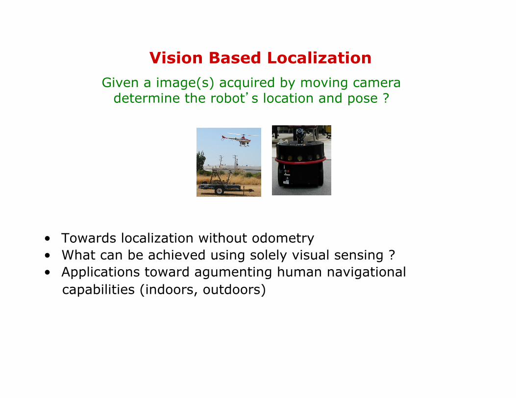
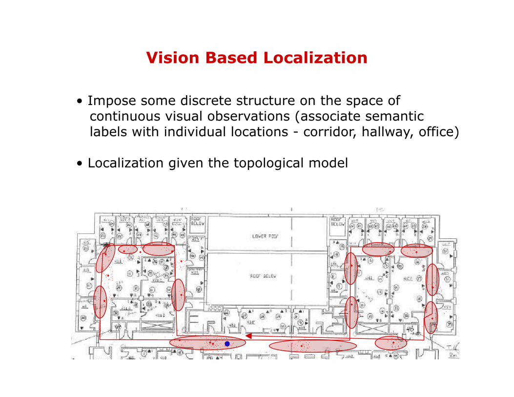
Vision Based Localization
• Towards localization without odometry • What can be achieved using solely visual sensing ? • Applications toward agumenting human navigational capabilities (indoors, outdoors)
Given a image(s) acquired by moving camera determine the robot’s location and pose ?
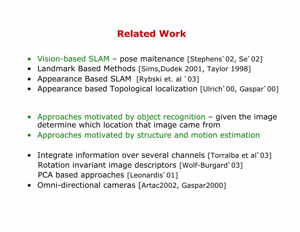
Related Work
• Vision-based SLAM – pose maitenance [Stephens’02, Se’02] • Landmark Based Methods [Sims,Dudek 2001, Taylor 1998] • Appearance Based SLAM [Rybski et. al ’03] • Appearance based Topological localization [Ulrich’00, Gaspar’00]
• Approaches motivated by object recognition – given the image
determine which location that image came from • Approaches motivated by structure and motion estimation • Integrate information over several channels [Torralba et al’03] Rotation invariant image descriptors [Wolf-Burgard’03] PCA based approaches [Leonardis’01] • Omni-directional cameras [Artac2002, Gaspar2000]

Challenges
• Metric and topological localization using only vision • Applicable to large scale self-similar environments • Robust to dynamic changes in the environment
Our Approach • Acquire video sequence during the exploration • Build the environment model in terms of locations and spatial relationships between them • Topological localization by means of location recognition • Metric localization by means of relative positioning
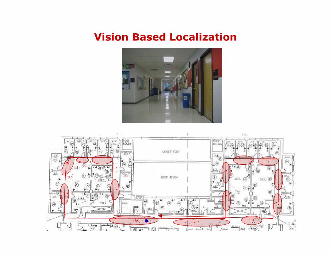
Vision Based Localization
Vision Based Localization
• Impose some discrete structure on the space of continuous visual observations (associate semantic labels with individual locations - corridor, hallway, office) • Localization given the topological model
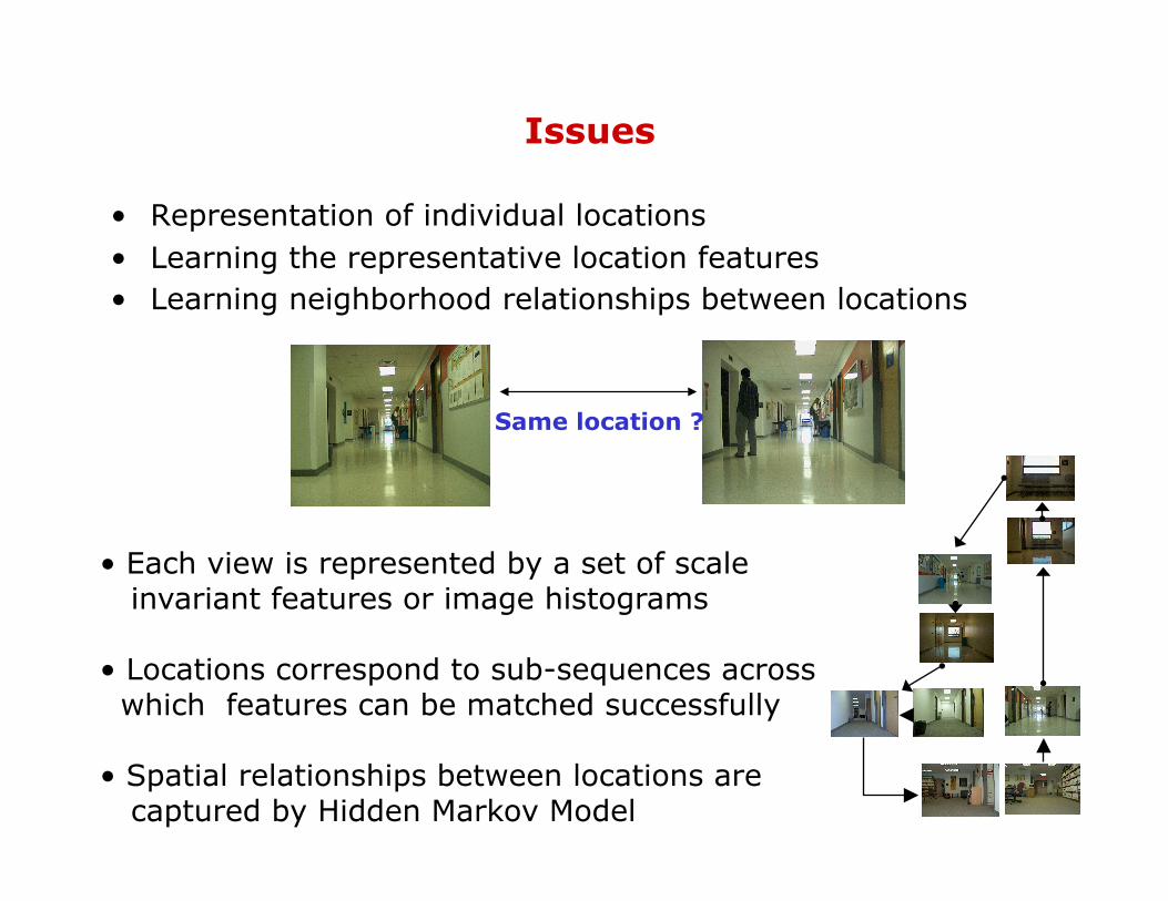
• Representation of individual locations • Learning the representative location features • Learning neighborhood relationships between locations
Same location ?
Issues
• Each view is represented by a set of scale invariant features or image histograms
• Locations correspond to sub-sequences across which features can be matched successfully • Spatial relationships between locations are captured by Hidden Markov Model

• Each image is characterized by a set of scale-invariant keypoints and their associated descriptors [D. Lowe,2000]
• Keypoints - extrema in DOG pyramid
• Descriptor – 8 bin orientation histograms computed over 4 x 4 grid overlayed over pixel neighbourhood and stacked together to form a 128 dim feature vector • Good repeatability across variations of scale and pose
Scale Invariant Features
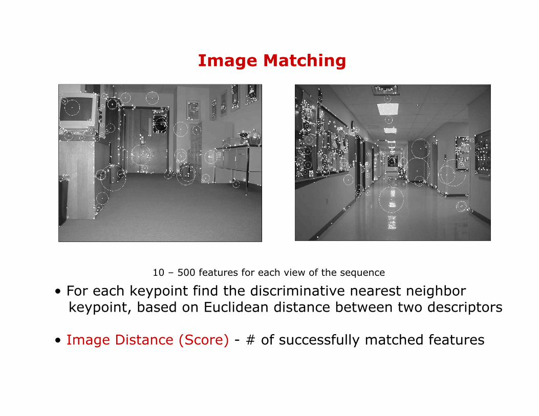
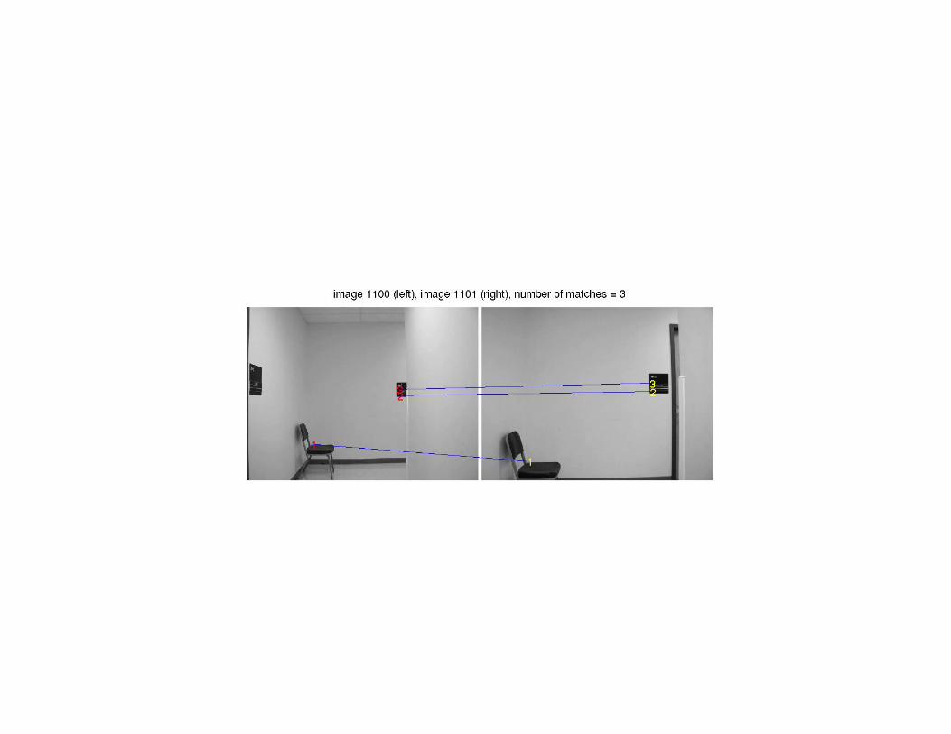
Image Matching
• For each keypoint find the discriminative nearest neighbor keypoint, based on Euclidean distance between two descriptors • Image Distance (Score) - # of successfully matched features
10 – 500 features for each view of the sequence

Partitioning the video sequence
• Transitions between individual locations determined during exploration • Location sub-sequence across which features can be
matched successfully (# of successfully matched features is lower then 2*minimal number of features needed for pose estimation)
• Location Representation - set of representative views and their associated keypoints
# of matched features 1st – i-th view
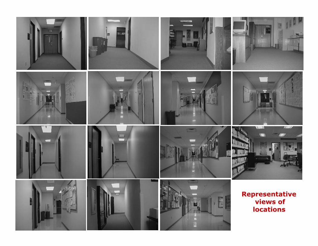
Representative views of locations
Location Recognition
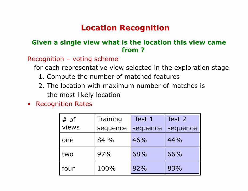
Given a single view what is the location this view came from ?
Recognition – voting scheme for each representative view selected in the exploration stage 1. Compute the number of matched features 2. The location with maximum number of matches is the most likely location • Recognition Rates
# of views
Training sequence
Test 1 sequence
Test 2 sequence
one 84 % 46% 44%
two 97% 68% 66%
four 100% 82% 83%

Location Recognition
• Large changes in the view point -> misclassification • Misclassification due to dynamic changes in the environment
• Exploit spatial relationships between individual locations to improve recognition
Markov Localization in the topological model
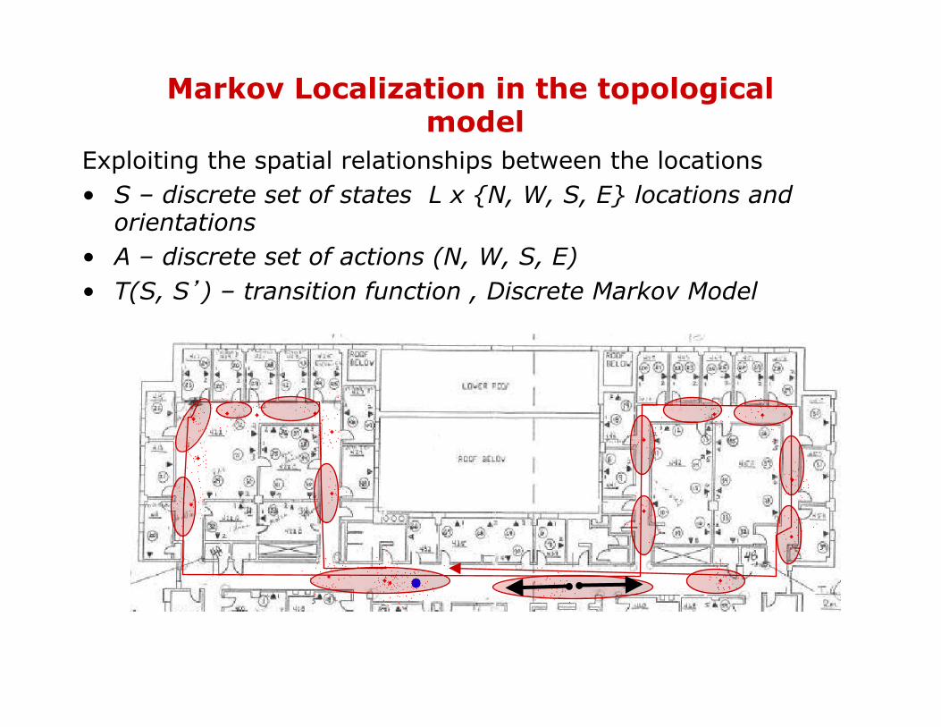
Exploiting the spatial relationships between the locations • S – discrete set of states L x {N, W, S, E} locations and
orientations • A – discrete set of actions (N, W, S, E) • T(S, S’) – transition function , Discrete Markov Model
Markov Localization in the topological model
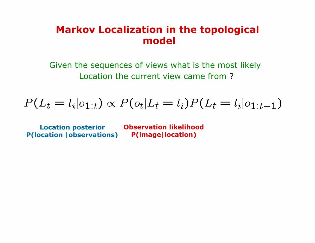
Given the sequences of views what is the most likely
Location the current view came from ?
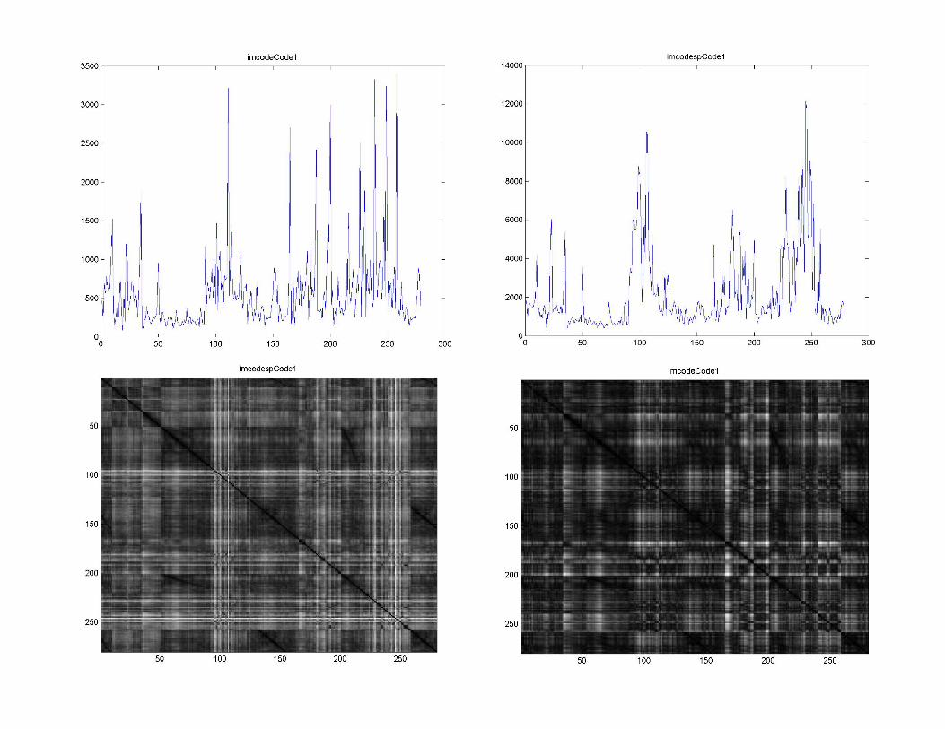
Observation likelihood P(image|location)
Location posterior P(location |observations)
# of successfully matched features
Location transition matrix

Markov Localization in the topological model
Given the sequences of views what is the most likely
Location the current view came from ?
Location posterior P(location |observations)
# of successfully matched features
Location transition probability matrix
Observation likelihood P(image|location)
Observation likelihood P(image|location)

• Slight digression

Time and uncertainty
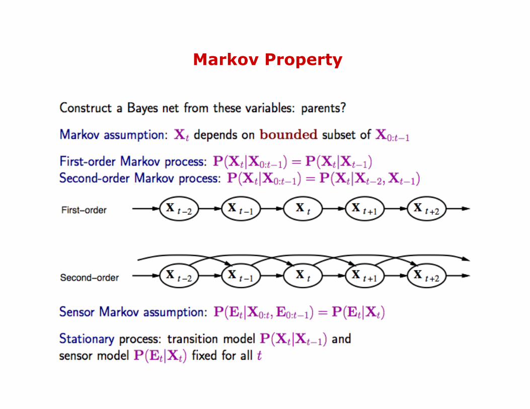
Markov Property

Inference Tasks
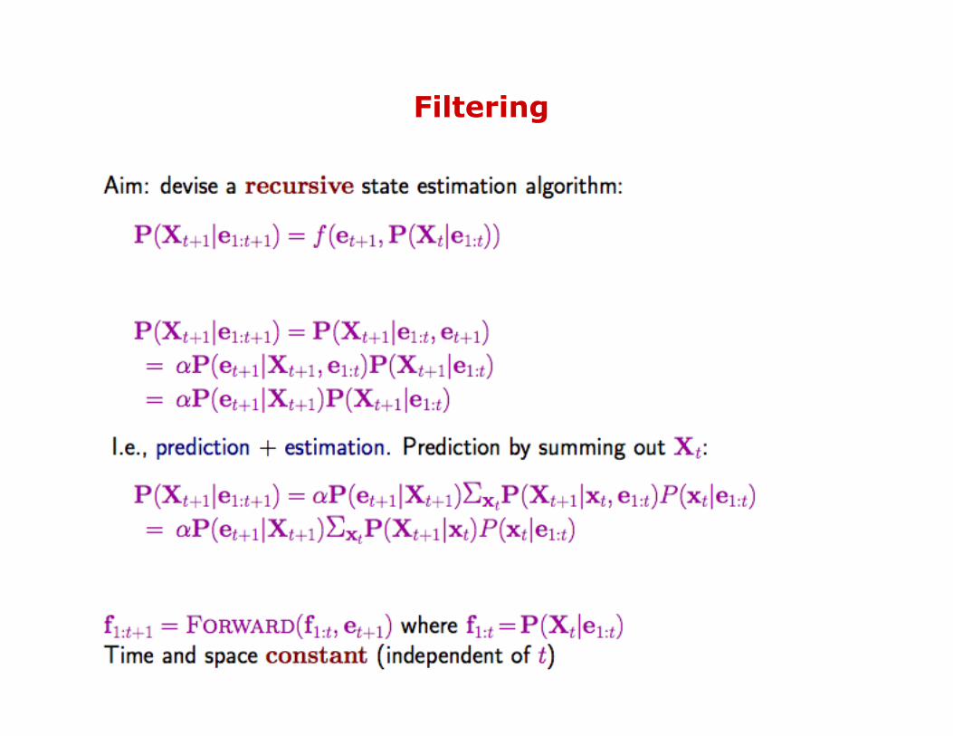
Filtering

Filtering Example
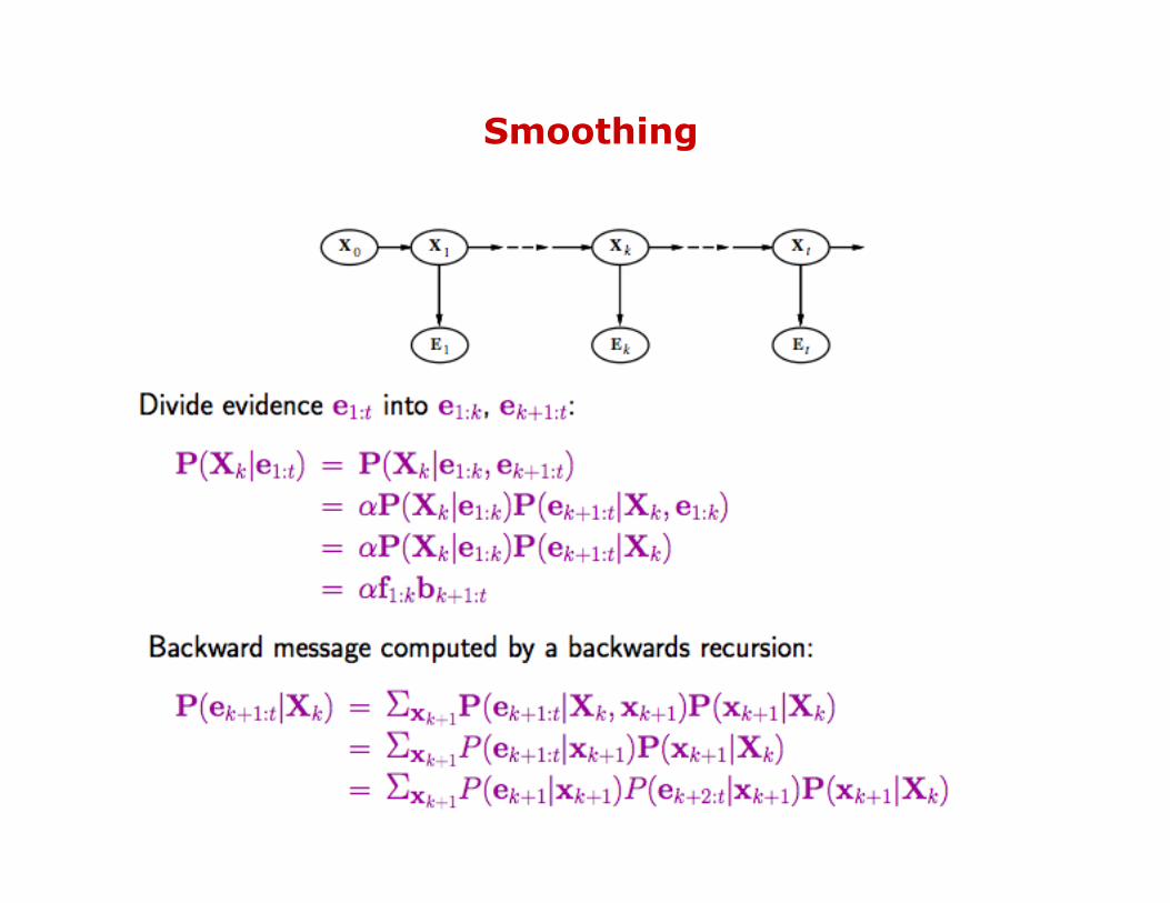
Smoothing
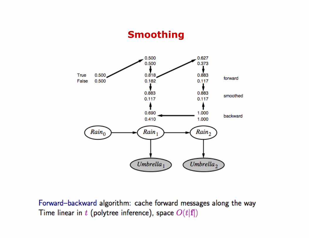
Smoothing
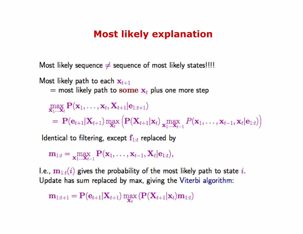
Most likely explanation
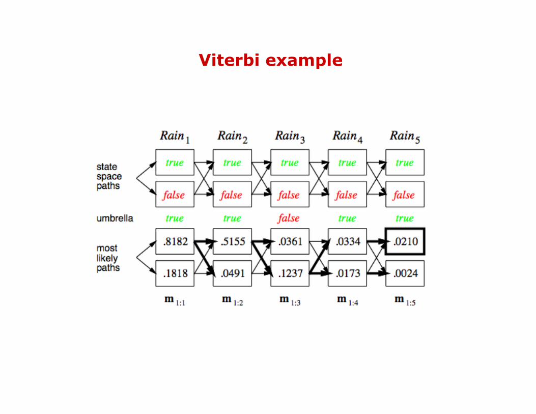
Viterbi example

Hidden Markov Models
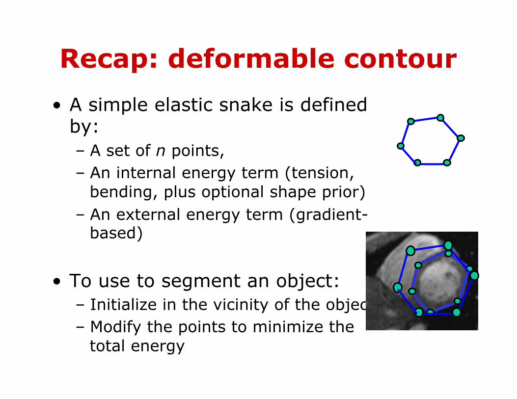
Recap: deformable contour
• A simple elastic snake is defined by: – A set of n points, – An internal energy term (tension,
bending, plus optional shape prior) – An external energy term (gradient-
based)
• To use to segment an object: – Initialize in the vicinity of the object – Modify the points to minimize the
total energy

Energy minimization: greedy
• For each point, search window around it and move to where energy function is minimal – Typical window size, e.g., 5 x 5 pixels
• Stop when predefined number of points have not changed in last iteration, or after max number of iterations
• Note: – Convergence not guaranteed – Need decent initialization
1v2v
3v
4v6v
5v
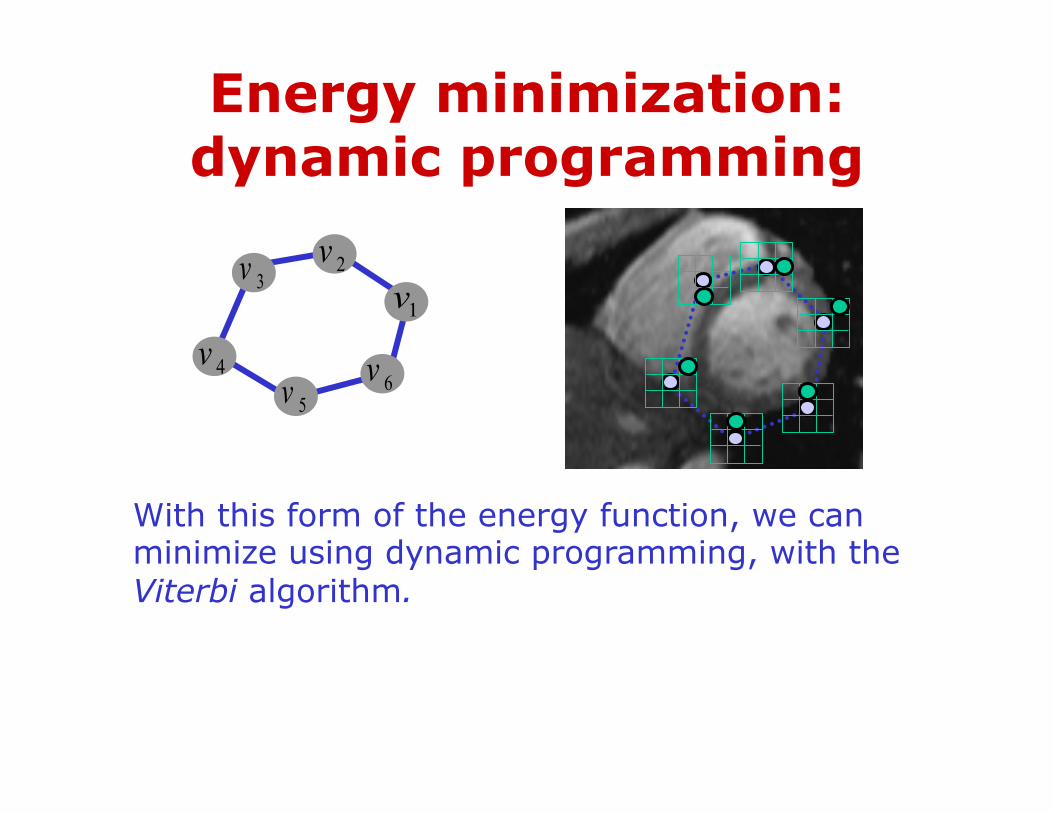
With this form of the energy function, we can minimize using dynamic programming, with the Viterbi algorithm.
Energy minimization: dynamic programming

Energy minimization: dynamic programming
∑−
=+=
1
111 ),(),,(
n
iiiintotal EE νννν…
• Possible because snake energy can be rewritten as a sum of pair-wise interaction potentials:
• Or sum of triple-interaction potentials.
∑−
=+−=
1
1111 ),,(),,(
n
iiiiintotal EE ννννν…

Snake energy: pair-wise interactions
21
1
211 |),(||),(|),,,,,( iiy
n
iiixnntotal yxGyxGyyxxE ∑
−
=
+−=……
21
1
1
21 )()( ii
n
iii yyxx −+−⋅+ +
−
=+∑α
∑−
=
−=1
1
21 ||)(||),,(
n
iintotal GE ννν… ∑
−
=+−⋅+
1
1
21 ||||
n
iii ννα
),(...),(),(),,( 113222111 nnnntotal vvEvvEvvEE −−+++=νν…212
1 ||||||)(||),( iiiiii GE νναννν −+−= ++where
Re-writing the above with :
( )iii yxv ,=

)3(3E
)(3mE )(4mE
)3(4E
)2(4E
)1(4E
)(mEn
)3(nE
)2(nE
)1(nE
)2(3E
)1(3E
)(2mE
)3(2E
)1(2E
)2(2E
0)1(1 =E
0)2(1 =E
0)3(1 =E
0)(1 =mE
Main idea: determine optimal position (state) of predecessor, for each possible position of self. Then backtrack from best state for last vertex.
states
1
2
…
m
vert
ices
1v 2v 3v 4v nv
)( 2nmOComplexity: vs. brute force search ____?
Viterbi algorithm

!"
!#$
=
>−=
.0 if )|()|(
,0 if ),()|()1,(max),(
00 kqxPqqP
kqxPqqPkjVjkiVieit
ikejit
The Viterbi Algorithm
€
φmax =argmaxφ i,L−1
V (i, L−1)Pt (q0 | qi )
sequence
stat
es
(i,k)
k k-1 . . .
k-2 k+1 . . . . . .
€
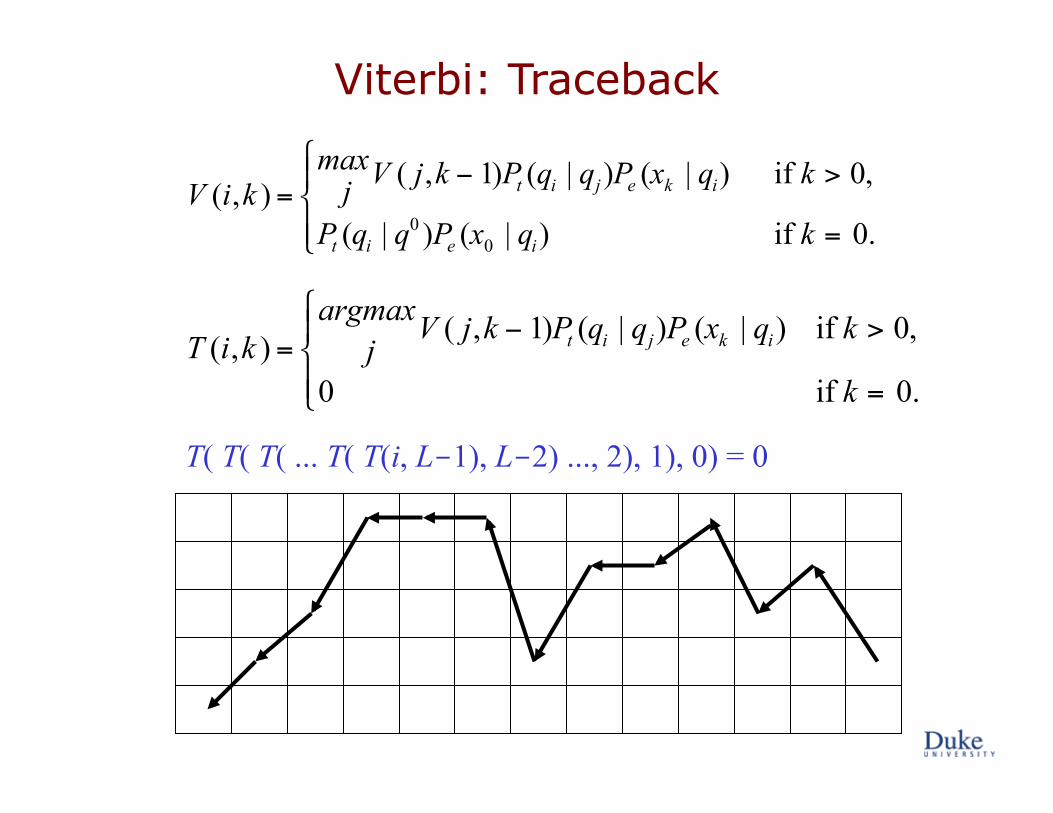
V (i,k ) =max
j V ( j,k − 1)Pt (qi | qj)Pe (xk | qi) if k > 0,
Pt (qi | q0 )Pe (x0 | qi) if k = 0.
# $ %
& %
€
T (i,k ) =argmax
jV ( j,k − 1)Pt (qi | qj)Pe (xk | qi) if k > 0,
0 if k = 0.
#
$ %
& %
Viterbi: Traceback
T( T( T( ... T( T(i, L-1), L-2) ..., 2), 1), 0) = 0
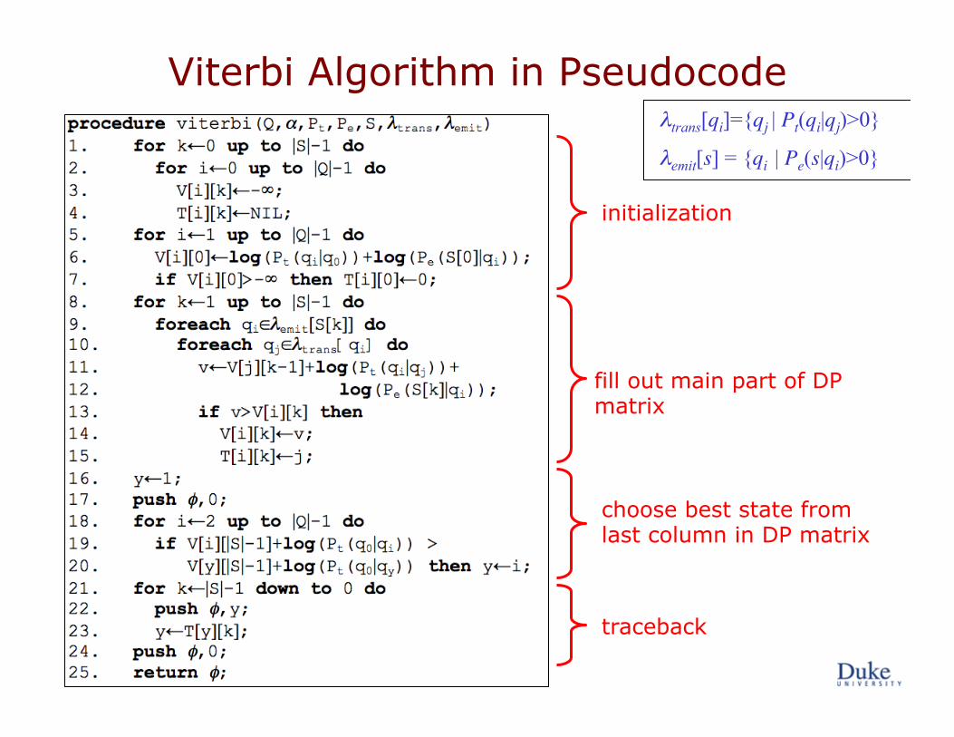
Viterbi Algorithm in Pseudocode λtrans[qi]={qj | Pt(qi|qj)>0}
λemit[s] = {qi | Pe(s|qi)>0}
initialization
fill out main part of DP matrix
choose best state from last column in DP matrix
traceback

HMM Recognition
96.3%
82%
95.4%
83%
With HMM
Without HMM

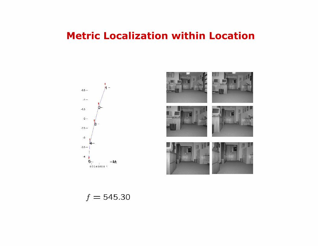
1. Given closest representative view of the location 2. Establish exact correspondences between keypoints 3. Matching combining (epipolar) geometry, keypoint descriptors and intrinsic scale 4. Compute relative pose with respect to the reference view (despite the unknown focal length)
Recovered relative displacements of new views
Representative view
Metric Localization within Location

Metric Localization within Location
Conclusions and Future Work
• Robust and effective categorization and automatic segmentation of video into distinct locations and distinct categories (indoors, outdoors, office, hallway, crossing)
• Topological and metric localization using scale invariant features • Extensions to outdoors environments (where the orientation cannot be coarsely quantized) • Develop complete exploration strategies • Enhancing matching and pose recovery methods for generic unstructured environments

Pose Estimation
• Two view epipolar geometry • Related Work [Sturm’01, Agapito’00, Ma et. al’03] • Calibrated case
• Essential matrix – planar case
• Partially calibrated case - unknown focal length

Pose Estimation
• Partially calibrated case - unknown focal length • Fundamental matrix
• Calibration constraints (Kruppa’s equations)
• With the epipole • In the planar motion case Kruppa’s equations can be renormalized with

Focal Length Estimation
• Planar Kruppa’s equations with
• Directly yields constraints on focal length
• can be estimated in the closed form

Robust Pose and Focal Length Estimation
• Modified random sampling strategy • Incorporates the focal length constraint (enables faster convergence) 1. Generate number of hypothesis by sampling 4 points
from the set of matches 2. Verify the which hypotheses satisfy the focal length
constraint 3. Select the hypothesis which minimizes the total
distance to the epipolar lines 4. Reject the matches with residual error above some
threshold

Sensitivity of the motion estimates
Simulation – 100 trials, different motion, error in correspondences measurements

1. Given closest representative view of the location 2. Establish exact correspondences between keypoints 3. Matching combining (epipolar) geometry, keypoint descriptors and intrinsic scale 4. Compute relative pose with respect to the reference view (despite the unknown focal length)
Recovered relative displacements of new views
Representative view
Metric Localization within Location
Metric Localization within Location

Conclusions and Future Work
• Robust and effective categorization and automatic segmentation of video into distinct locations and distinct categories (indoors, outdoors, office, hallway, crossing)
• Topological and metric localization using scale invariant features • Exploit geometric relationships between features • Alternative features/feature descriptors • Extensions to outdoors environments
• Develop complete exploration strategies • Improving the matching and pose recovery methods for generic unstructured environments
Related Documents