topographic data and roughness parameterisation effects

Department of Technology and Built Environment

TOPOGRAPHIC DATA AND ROUGHNESS PARAMETERISATION EFFECTS ON 1D FLOOD INUNDATION MODELS

Nancy Joy Lim

June 2009

Geomatics Programme Bachelor’s Thesis in Geography

Supervisor: S. Anders Brandt Examinator: Bo Malmström

Co-examinator: Peter Fawcett

ii

iii

ABSTRACT

A big responsibility lies in the hand of local authorities to exercise measures in preventing fatalities and damages during flood occurrences. However, the problem is how flooding can be prevented if nobody knows when and where it will be occurring, and how much water is expected. Therefore, the utilisation of flood models in such studies can be helpful in simulating what is anticipated to occur. In this study, the HEC-RAS steady flow model was used in calibrating different flood events in Testeboån river, which is situated in the municipality of Gävle in Sweden. The purpose is to provide inundation maps that show the water surface profiles for the various flood events that can help authorities in planning within the area. Moreover, the study would try to address certain issues, which concern one-dimensional models like HEC-RAS in terms of the effects of topographic data and the parameters used for friction coefficient. Various flood maps were produced to visualise the extents of the floods. In Oppala and Norra Åbyggeby, the big water extents for both the 100-year and the highest probable floods were visible in the forested areas and grasslands, although a few houses were within the predicted flooded areas. In Södra Åbyggeby, Varva, Forsby, and in the northern parts of Strömsbro and Stigslund, the majority of the residential places were not inundated during the 100-year flood calibration, but became flooded during the maximum probable flood. The southern portions of Strömsbro and Stigslund had lesser flood extents and houses were situated within the boundaries of the highest flood. In Näringen, there were also some areas close to the estuary that were flooded for both events. With the other calibrations performed, two factors that greatly affect the flood extents in the floodplain, particularly in flatter areas were topographic data and the parameters used as friction coefficient. The use of high resolution topographic data was important in improving the performance of the software. Nevertheless, it must be emphasised that in areas characterised by gentler slopes that bounded the channel and the floodplain, data completeness became significant whereby both ground data and bathymetric points must be present to avoid overestimation of the inundation extent. The water extents also varied with the use of the various Manning’s n for the overbanks, with the bigger value showing greater water extents. Else, in areas with steeper slopes and where the water was confined to the banks, the effect was minimal. Despite these shortcomings of one-dimensional models, HEC-RAS provided good inundation extents that were comparable to the actual extent of the 1977 flooding. Modelling real floods has its own difficulties due to the unpredictability of real-life flood behaviours, and more especially, there are time dependent factors that are involved. Although calibrating a flood event will not exactly determine what is to arise as they might either under- or overestimate such flooding occurrences, still, they give a standpoint of what is more or less to anticipate, and from this, planning measures can be undertaken. Keywords: flood, GIS, HEC-RAS, inundation study, one-dimensional flood model, topographic data, roughness coefficient

iv

PREFACE

The thesis was done in cooperation with Gävle Municipality as part of creating flood inundation maps for

Testeboån river that could visualise possible water extents during the different flood events. Likewise, the

paper would also try to address some of the issues in simulating floods using one-dimensional flood models

such as the HEC-RAS steady-flow analysis, as they were encountered in the study. Through this, such problems

could serve as bases for future studies to further investigate that could lead to the improvement of the

software’s performance, as well as the quality of results produced by it. In return, such improvements could

benefit planners and authorities in the overall decision-making process when these outputs are applied as part

of planning measures to be implemented in real-life circumstances.

This study would not be possible without the help of the people who supported me all throughout the time I

worked on the thesis. My sincerest gratitude to my supervisor, Anders Brandt, for all the advise and ideas he

imparted, as well as for all the help I received since I began studying in the University of Gävle. I would also like

to show my appreciation to Fredrik Ekberg and to all other people from the Municipality of Gävle for all the

assistance, particularly whenever I needed help which regards to Testeboån. Special thanks as well to Magnus

Petterson of SWECO, Else-Marie Wingqvist of SMHI, Bo Malmström, Peter Fawcett and Scarlett Jiang. Last but

not the least, to my family for all the support.

Gävle, May 2009

Nancy Joy Lim

v

TABLE OF CONTENTS

INTRODUCTION ....................................................................................................................................................... 1

Background ......................................................................................................................................................... 1

Aims of the Study ............................................................................................................................................... 1

PREVIOUS RESEARCH ON FLOOD MODELING ......................................................................................................... 2

Flood Simulation Models: 1D vs. 2D Models ...................................................................................................... 2

Topographic data and roughness parameterization in 1D models .................................................................... 2

HEC-RAS steady-flow simulation ........................................................................................................................ 3

STUDY AREA AND HISTORICAL FLOOD RECORDS .................................................................................................... 4

MATERIALS AND METHODS .................................................................................................................................... 5

Pre-processing of Topographic Data .................................................................................................................. 5

Computation based on known depths ........................................................................................................... 6

Computation of unknown depths ................................................................................................................... 9

Land Use Map Creation .................................................................................................................................... 12

Derivation of HEC-RAS Data ............................................................................................................................. 14

Hydraulic Simulation ......................................................................................................................................... 15

Flood Delineation ............................................................................................................................................. 16

Calibration ........................................................................................................................................................ 16

RESULTS ................................................................................................................................................................ 17

Actual Flood vs. HEC-RAS result ....................................................................................................................... 23

Assessing the effects of using complete and incomplete topographic data .................................................... 27

Calibration of different Manning’s n values for the left- and right overbanks ................................................. 29

Comparison with SMHI Results ........................................................................................................................ 32

DISCUSSION ........................................................................................................................................................... 35

CONCLUSION ......................................................................................................................................................... 37

REFERENCES .......................................................................................................................................................... 37

Appendix A: Nomenclature ................................................................................................................................... 40

Appendix B: Summary of parameters used in the calibrations ............................................................................. 41

Appendix C: Glossary ............................................................................................................................................ 42

Appendix D: Computed new depths ..................................................................................................................... 44

Appendix E: Inundation maps with water levels ................................................................................................... 46

Appendix F: File listing .......................................................................................................................................... 52

vi

LIST OF FIGURES

Figure 1. Map of the Study Area................................................................................................................... 4

Figure 2. Locations with unknown river bathymetric points........................................................................ 6

Figure 3. Positioning of cross-sections based on known points................................................................... 7

Figure 4. River’s cross-sectional area as represented by depth [d] and width [w]....................................... 7

Figure 5. Sample plot of computed depth data............................................................................................ 11

Figure 6. Combined data points for a selected portion of the study area.................................................... 12

Figure 7. TIN model of the selected area as Figure 5................................................................................... 12

Figure 8. Land use map used for the study with the corresponding Manning’s n values shown in

Figure 3.........................................................................................................................................

13

Figure 9. Different HEC-RAS themes generated for the study...................................................................... 14

Figure 10. Cross-sections created for the study area and the SMHI cross-sections..................................... 15

Figure 11. Inundation extents for the different flood events....................................................................... 17

Figure 12. Water surface profiles for normal water discharge, the 100-year flood and the highest

probable flood.............................................................................................................................

18

Figure 13. Areas mapped with water extending behind the bank lines using the normal discharge rate... 18

Figure 14. Cross-section profiles of the inundated area in the estuary........................................................ 19

Figure 15. The 100-yr flood and the maximum probable flood’s extents in Oppala and Norra Åbyggeby.. 19

Figure 16. The 100-yr flood and the maximum probable flood’s extents in Södra Åbyggeby and Norra

Åbyggeby.....................................................................................................................................

20

Figure 17. The 100-yr flood and the maximum probable flood’s extents in Varva, Strömsbro, Forsby and

Stigslund......................................................................................................................................

21

Figure 18. The 100-yr flood and the maximum probable flood’s extents in Strömsbro and Stigslund (a)

and Näringen (b)........................................................................................................................

22

Figure 19. Actual flood extent against the simulated inundation from HEC-RAS......................................... 23

Figure 20. Simulated inundation extents of the middle sections of the river compared to the 1977’s

flood extent.................................................................................................................................

24

Figure 21. Variations in the flood extent between the actual map and the HEC-RAS result for one of the

central areas of the river.............................................................................................................

25

Figure 22. Flood extents between the 1977 flood and the HEC-RAS output in two other areas................. 25

Figure 23. Elevation comparison of inner areas that were not inundated in the HEC-RAS result................ 26

Figure 24. Elevation comparison of inner areas that were not inundated in HEC-RAS result...................... 27

Figure 25. Flood extents using complete and incomplete topographic data, as against the actual flood

map in areas with interpolated bathymetric data.......................................................................

28

vii

Figure 26. Flood extents using different topographic data in areas characterised by steeper bank slopes

with interpolated bathymetric data............................................................................................

28

Figure 27. Flood extents using complete and incomplete topographic data, against the actual flood map

in flat floodplains, with surveyed bathymetric points.................................................................

29

Figure 28. Flood extents using different Manning’s n in flat floodplains..................................................... 30

Figure 29. Flood extents using different Manning’s n in areas with steeper areas...................................... 31

Figure 30. Flood extents from the newly simulated flood as against the SMHI result, where

Q = 165 m3/s………………………………………………………………………………………………………………………………………....

32

Figure 31. Flood extents from the newly simulated flood as against the SMHI result, where Q = 386 m3/s 33

Figure 32. Simulated flood extents vs. Actual Flooding extents................................................................... 34

Figure 33. Misrepresented areas by the SMHI result................................................................................... 35

LIST OF TABLES

Table 1. Computed values for the cross-sections with known river elevations........................................... 9

Table 2. Computed depths based on the hydraulic radius of the upstream cross-section, and the

corresponding new river elevations................................................................................................

10

Table 3. Land use classification with corresponding Manning’s n values..................................................... 13

Table 4. Discharge rates for different flood events (SMHI, 2007)................................................................ 16

viii

INTRODUCTION

Background

Historically, floods have been an integral part of the processes taking place in the natural surrounding; yet, can be one of the most catastrophic in terms of the damages and inconveniences that they bring about to human lives and the environment (Mays, 2001). They may occur along bodies of water, such as rivers, lakes, small streams, and coastal areas, or in alluvial fans, or even in areas with poor drainage system (Mays, 2001). However, it is difficult to predict when they will be occurring or how much water is expected during a particular flood event. Causes of floods can vary from place to place. In Sweden, flooding can be due to heavy rains or snow melts, but the more dangerous ones can be attributed to a combination of factors instigating each other, such as too much snow throughout the winter, causing more snow to melt in the spring season (SMHI, 2004). This is evident in the northern parts of the country where the snow melts in the higher altitude and forested areas during the said season, contributing to torrential waters coming from higher to lower places, and this can be further worsened by additional rainfalls (SMHI, 2004). One of the biggest recorded floodings of the 20

th century in the country occurred in the spring of 1995, in

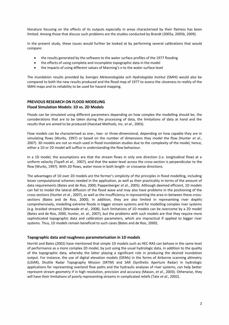
Norrland and north of Svealand wherein snow had been excessive during the winter season and the melting in the forests had been delayed for several weeks than what had been expected. This caused an intensive melting of snow from the forests and the mountains that was further hastened by the sudden increase in temperature. Several days later, rain occurred adding up to the already high waters of the rivers, specifically in Vindelälven and Piteälven. Many properties close to these rivers, including residences and summer houses had been damaged, in addition to roads and bridges, especially in places where such flood were not foreseen to occur (SMHI, 2004). With the present changes in climate attributed to global warming, extreme weather conditions can occur any time, that may lead to big floods even in places where they are least anticipated. In Gävle, it is recognised that climate change will be bringing about warmer winter, with less snow but wetter season, characterised by heavy rains. Flooding is predicted to be caused by such heavy downpours, rather than snow melts that previously occurred during the spring seasons (Gävle Kommun, 2007). Inundation or floodplain studies are widely used and valuable for such purposes to give an overview of water surface profiles in terms of maps, not only in flood prone areas, but in areas close to bodies of water (Haestad Methods, Inc. et al., 2003). Such studies can incorporate the analysis of past flood events or the estimation of the water surface profile for the 100-year flood that can be calibrated, with the aid of specialised software specifically designed for hydraulic analysis. Together with the current developments in geographic information systems (GIS), hydraulic analysis had been modernised and can yield more accurate outcomes and details in the models (Haestad Methods, Inc. et al., 2003). Yet, such simulation models, particularly the Hydrologic Engineering Center’s River Analysis System (HEC-RAS) has its own issues that have to be addressed prior to improving its performance in giving out the desired inundation extents. The two most common problems concern topographic data resolution and the parameters used for friction coefficient.

Aims of the Study

This study aims to predict possible flood outcomes in Testeboån river in Gävle, Sweden for the different flood events, with the utilisation of GIS and HEC-RAS steady-flow analysis model. The research’s output maps that would show the inundation extents are intended to aid in the future planning of the area, as well as in the decision-making process of concerned authorities in the municipality. Moreover, the thesis’ output would also try to contribute to the comprehension of the behaviour of one-dimensional flood models like HEC-RAS, particularly its sensitivity to both topographic data and roughness coefficient in flatter areas. Although topographic data and Manning’s n are recognised by many experts in the field to affect the performance of the software in terms of the results that they produce (Horritt and Bates, 2001; Pappenberger, et al., 2005; Brandt, 2005a, 2005b, 2009; Casas, et al., 2006; Hunter et al., 2007),

1

2

literature focusing on the effects of its outputs especially in areas characterised by their flatness has been limited. Among those that discuss such problems are the studies conducted by Brandt (2005a, 2005b, 2009). In the present study, these issues would further be looked at by performing several calibrations that would compare:

the results generated by the software to the water surface profiles of the 1977 flooding

the effects of using complete and incomplete topographic data in the model

the impacts of using different values of Manning’s n to the water surface level The inundation results provided by Sveriges Meteorologiska och Hydrologiska Institut (SMHI) would also be compared to both the new results produced and the flood map of 1977 to assess the closeness to reality of the SMHI maps and its reliability to be used for hazard mapping.

PREVIOUS RESEARCH ON FLOOD MODELING Flood Simulation Models: 1D vs. 2D Models

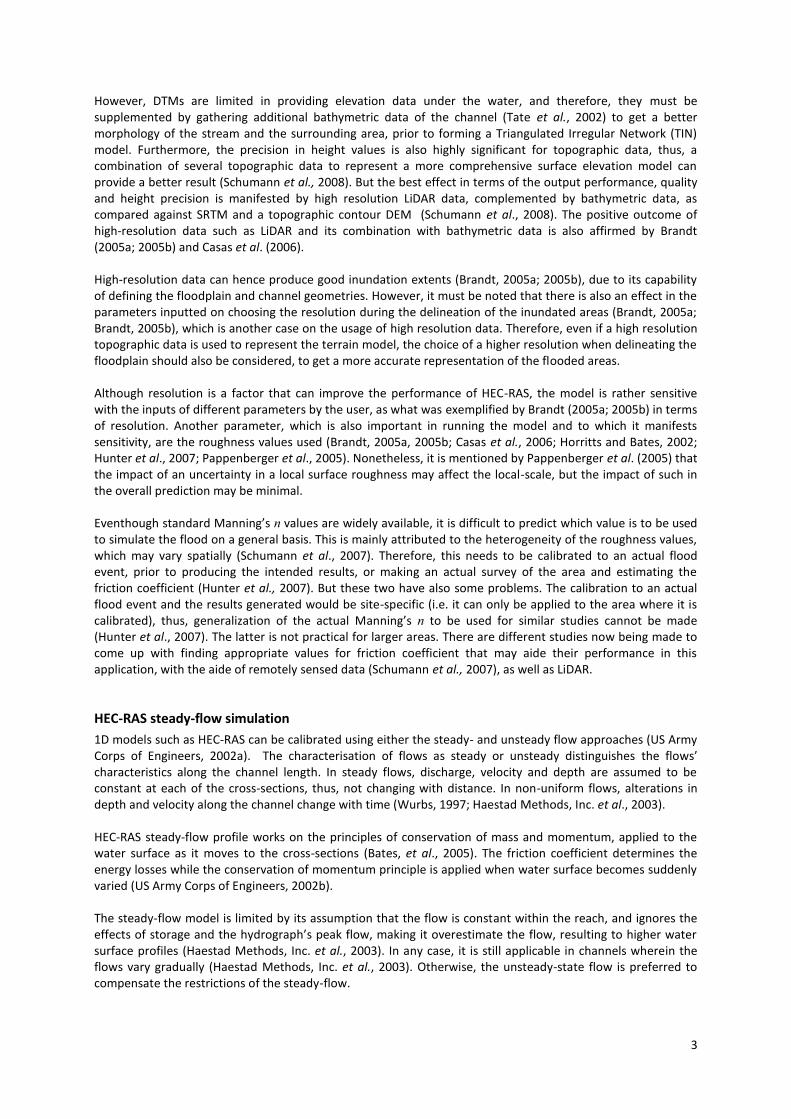
Floods can be simulated using different parameters depending on how complex the modelling should be, the considerations that are to be taken during the processing of data, the limitations of data at hand and the results that are aimed to be produced (Haestad Methods, Inc. et al., 2003). Flow models can be characterised as one-, two- or three-dimensional, depending on how capable they are in simulating flows (Wurbs, 1997) or based on the number of dimensions they model the flow (Hunter et al., 2007). 3D models are not so much used in flood inundation studies due to the complexity of the model, hence, either a 1D or 2D model will suffice in understanding the flow behaviour. In a 1D model, the assumptions are that the stream flows in only one direction (i.e. longitudinal flow) at a uniform velocity (Tayefi et al., 2007), and that the water-level across the cross-section is perpendicular to the flow (Wurbs, 1997). With 2D flows, water move in both length- or crosswise directions. The advantages of 1D over 2D models are the former’s simplicity of the principles in flood modelling, including lesser computational schemes needed in the application, as well as their practicality in terms of the amount of data requirements (Bates and de Roo, 2000; Pappenberger et al., 2005). Although deemed efficient, 1D models can fail to model the lateral diffusion of the flood wave and may also have problems in the positioning of the cross-sections (Hunter et al., 2007), as well as the insufficiency in representing the area in-between these cross-sections (Bates and de Roo, 2000). In addition, they are also limited in representing river depths comprehensively, modelling extreme floods in bigger stream systems and for modelling complex river systems (e.g. braided streams) (Merwade et al., 2008). Such limitations of 1D models can be overcome by a 2D model (Bates and de Roo, 2000, Hunter, et. al., 2007), but the problems with such models are that they require more sophisticated topographic data and calibration parameters, which are impractical if applied to bigger river systems. Thus, 1D models remain beneficial to such cases (Bates and de Roo, 2000).

Topographic data and roughness parameterisation in 1D models

Horritt and Bates (2002) have mentioned that simple 1D models such as HEC-RAS can behave in the same level of performance as a more complex 2D model, by just using the usual hydrologic data, in addition to the quality of the topographic data, whereby the latter playing a significant role in producing the desired inundation output. For instance, the use of digital elevation models (DEMs) in the forms of Airborne scanning altimetry (LiDAR), Shuttle Radar Topography Mission (SRTM) and SAR (Synthetic Aperture Radar) in hydrologic applications for representing overland flow paths and the hydraulic analyses of river systems, can help better represent stream geometry if in high resolution, precision and accuracy (Mason, et al., 2003). Otherwise, they will have their limitations of poorly representing streams in complicated reliefs (Tate et al., 2002).

3

However, DTMs are limited in providing elevation data under the water, and therefore, they must be supplemented by gathering additional bathymetric data of the channel (Tate et al., 2002) to get a better morphology of the stream and the surrounding area, prior to forming a Triangulated Irregular Network (TIN) model. Furthermore, the precision in height values is also highly significant for topographic data, thus, a combination of several topographic data to represent a more comprehensive surface elevation model can provide a better result (Schumann et al., 2008). But the best effect in terms of the output performance, quality and height precision is manifested by high resolution LiDAR data, complemented by bathymetric data, as compared against SRTM and a topographic contour DEM (Schumann et al., 2008). The positive outcome of high-resolution data such as LiDAR and its combination with bathymetric data is also affirmed by Brandt (2005a; 2005b) and Casas et al. (2006). High-resolution data can hence produce good inundation extents (Brandt, 2005a; 2005b), due to its capability of defining the floodplain and channel geometries. However, it must be noted that there is also an effect in the parameters inputted on choosing the resolution during the delineation of the inundated areas (Brandt, 2005a; Brandt, 2005b), which is another case on the usage of high resolution data. Therefore, even if a high resolution topographic data is used to represent the terrain model, the choice of a higher resolution when delineating the floodplain should also be considered, to get a more accurate representation of the flooded areas. Although resolution is a factor that can improve the performance of HEC-RAS, the model is rather sensitive with the inputs of different parameters by the user, as what was exemplified by Brandt (2005a; 2005b) in terms of resolution. Another parameter, which is also important in running the model and to which it manifests sensitivity, are the roughness values used (Brandt, 2005a, 2005b; Casas et al., 2006; Horritts and Bates, 2002; Hunter et al., 2007; Pappenberger et al., 2005). Nonetheless, it is mentioned by Pappenberger et al. (2005) that the impact of an uncertainty in a local surface roughness may affect the local-scale, but the impact of such in the overall prediction may be minimal. Eventhough standard Manning’s n values are widely available, it is difficult to predict which value is to be used to simulate the flood on a general basis. This is mainly attributed to the heterogeneity of the roughness values, which may vary spatially (Schumann et al., 2007). Therefore, this needs to be calibrated to an actual flood event, prior to producing the intended results, or making an actual survey of the area and estimating the friction coefficient (Hunter et al., 2007). But these two have also some problems. The calibration to an actual flood event and the results generated would be site-specific (i.e. it can only be applied to the area where it is calibrated), thus, generalization of the actual Manning’s n to be used for similar studies cannot be made (Hunter et al., 2007). The latter is not practical for larger areas. There are different studies now being made to come up with finding appropriate values for friction coefficient that may aide their performance in this application, with the aide of remotely sensed data (Schumann et al., 2007), as well as LiDAR.

HEC-RAS steady-flow simulation

1D models such as HEC-RAS can be calibrated using either the steady- and unsteady flow approaches (US Army Corps of Engineers, 2002a). The characterisation of flows as steady or unsteady distinguishes the flows’ characteristics along the channel length. In steady flows, discharge, velocity and depth are assumed to be constant at each of the cross-sections, thus, not changing with distance. In non-uniform flows, alterations in depth and velocity along the channel change with time (Wurbs, 1997; Haestad Methods, Inc. et al., 2003). HEC-RAS steady-flow profile works on the principles of conservation of mass and momentum, applied to the water surface as it moves to the cross-sections (Bates, et al., 2005). The friction coefficient determines the energy losses while the conservation of momentum principle is applied when water surface becomes suddenly varied (US Army Corps of Engineers, 2002b). The steady-flow model is limited by its assumption that the flow is constant within the reach, and ignores the effects of storage and the hydrograph’s peak flow, making it overestimate the flow, resulting to higher water surface profiles (Haestad Methods, Inc. et al., 2003). In any case, it is still applicable in channels wherein the flows vary gradually (Haestad Methods, Inc. et al., 2003). Otherwise, the unsteady-state flow is preferred to compensate the restrictions of the steady-flow.

4

STUDY AREA AND HISTORICAL FLOOD RECORDS The whole stretch of Testeboån channel is about 85 km long, from Åmot in Ockelbo municipality downstream to its drainage in Gävle. For the purpose of this study, the focus area would only be covering the part of the river within the municipality of Gävle, i.e. from the E4 motorway downstream to its delta (Figure 1).

Figure 1. Map of the Study Area (Gävle Kommun, 2008)

The river lies on a flat and blocky moraine countryside. Its upstream part has still its underlying bedrock. The entire river stretch is considered to be rich with running water carrying sediment derived from moraine. The important areas of the flat surfaces surrounding the river, especially in the upstream and within the so-called Inre Fjärden, are covered with sand and clay released by the river during high water periods (Bonde and Ståhl, 1995). From the E4 motor highway, downstream, the river is composed of a single-thread stream. It is surrounded mostly by coniferous forests, lined with deciduous forests. Broad leaf trees are scattered in different places, and along the river are some cleared areas. In Strömsbro, specifically at the bridge called Lexvallsbron, the eastern part of Testeboån is characterised by high and steep river banks. This portion of the river gets in contact with glaciofluvial deposits. While in other places, the stream runs through the flat and more often blocky moraine landscape of the municipality (Torung, 2006). The western portion of the river in Stigsgård is covered by old pine trees estimated to be 400 years old, while at the upstream portion of Oskarbron, the river is lined with abundant deciduous trees (Torung, 2006). The delta, where the estuary is situated, is a deposition of sand. In the part called Avasätorna, about 25 ha of wetlands exist (Testeboliv, 2008). Testeboån delta is a natural reserved area under the Natura-2000 project. Much effort has been made by the municipality in preserving and protecting this section of the channel. In the 20

th century, there were four recorded great flooding occurrences that took place in the Gävle area,

affecting Testeboån. These occurred in the years 1916 (177 m3/s), 1937 (127 m

3/s), 1966 (180 m

3/s) (Olofsson

and Berggren, 1966) and 1977 (160 m3/s). All of these floods happened during the spring season.

One of the earlier writings published concerning the study of the floods in Testeboån was undertaken by Olofsson and Berggren (1966), wherein they investigated the behaviour of the river during extreme flood events through observations, as well as analysing historical maximum discharges and their corresponding water levels.

E4 motorway

delta

5

In 2002, as part of its series of flood inundation studies, SMHI, as commissioned by the Swedish Rescue Agency (Räddningsverket), had published a report with the title Översiktlig översvämningskartering längs Testeboån: sträckan från Åmot till utloppet i Bottenhavet. SMHI simulated both the 100-year flood for the river and the maximum probable flood event using the Mike-11 software. The topographic data utilised came from the National Land Surveying Office’s GSD elevation data, having a resolution of 50 metres.

MATERIALS AND METHODS

The primary topographic data that was used in the study were laser-scanned data and river elevation points produced by SWECO. The laser scan survey was undertaken on 5 May 2008. Total number of points gathered from the survey was 166 million points, of which, 47 million comprised the ground points, and the remaining points constituted the different vegetations, buildings and other unclassified objects. The model key points, which were the filtered ground points that were used as the main ground data for the study, consisted of 4 million points. This data had an accuracy of 0.10 m horizontally. The river bathymetric data were derived through echo sounding survey from October 22-25 and 27, 2008 using GPS. Approximately 30,000 points were derived from the survey. Nevertheless, there were some parts of the river, which were too shallow to be surveyed with echo sounding; therefore, these parts had missing river elevation data. Additional depth data were also provided by the municipality of Gävle for the estuary. All the topographic data from Sweco were delivered in ASCII format. A separate orthophoto data for the entire area was also included in their delivery. The additional depth dataset for the estuary was given in shape file. Other data used such as the land cover map and other maps of the area that were used in the creation of the land use map were provided by the municipality, as well as the map showing the extents of the 1977 flooding. In addition, they also provided the shape file output of the inundation results by SMHI, as well as the cross-section data that had been used. A complete listing of the datasets derived and used for the study may be seen in Appendix F. The main software utilised were ESRI’s Arcview 3.3 and the Hydrologic Engineer Center’s River Analysis System (HEC-RAS). The former was used with the HEC-Geo RAS extension for the pre-processing of the topographic data, the creation of the geometric data for the channel, as well as in flood delineation. The HEC-RAS model was employed for the simulation of the different flood events. Secondary data such as scientific papers/journals, books and internet websites were also utilised to provide an overall understanding of the topic at hand, and as bases for all the information that were used for the study.

Pre-processing of Topographic Data

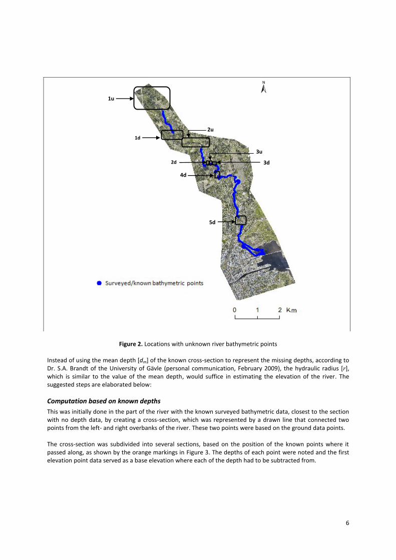
In the locations with the absence of bathymetric data, depths had to be estimated based on the known ones. These sections of the river with the missing elevations are shown in Figure 2, whereby their locations were coded as upstream (u) and downstream (d) to facilitate finding the positions of points to be added for the later computations.

6

Figure 2. Locations with unknown river bathymetric points

Instead of using the mean depth [dm] of the known cross-section to represent the missing depths, according to Dr. S.A. Brandt of the University of Gävle (personal communication, February 2009), the hydraulic radius [r], which is similar to the value of the mean depth, would suffice in estimating the elevation of the river. The suggested steps are elaborated below:

Computation based on known depths

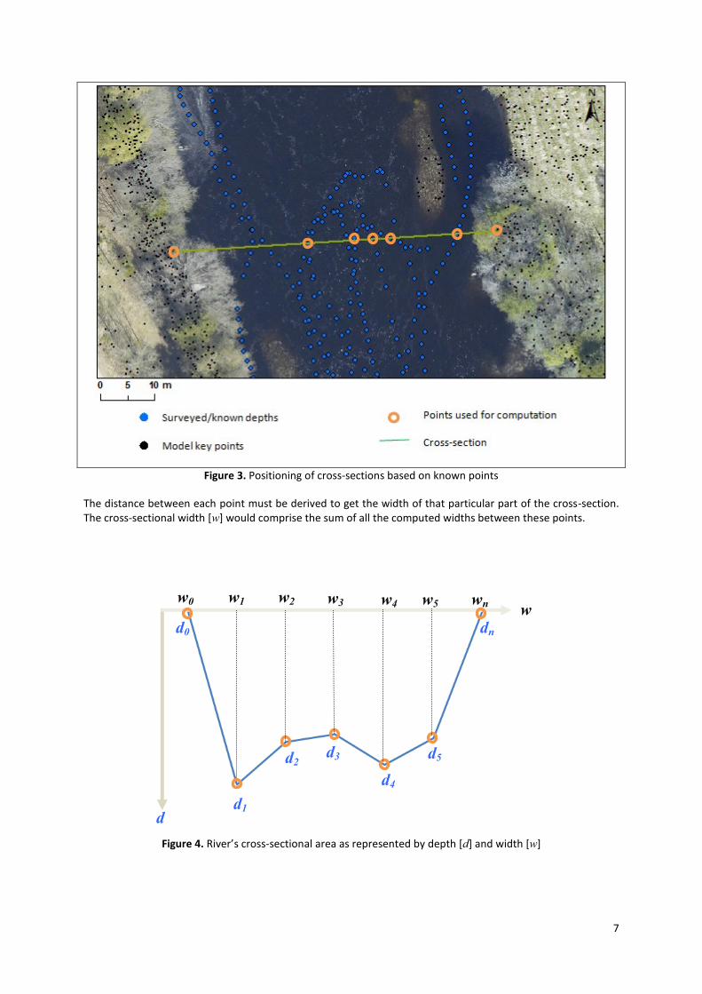
This was initially done in the part of the river with the known surveyed bathymetric data, closest to the section with no depth data, by creating a cross-section, which was represented by a drawn line that connected two points from the left- and right overbanks of the river. These two points were based on the ground data points. The cross-section was subdivided into several sections, based on the position of the known points where it passed along, as shown by the orange markings in Figure 3. The depths of each point were noted and the first elevation point data served as a base elevation where each of the depth had to be subtracted from.

2u

3u

1u

1d

3d

4d

5d

2d

7

Figure 3. Positioning of cross-sections based on known points

The distance between each point must be derived to get the width of that particular part of the cross-section. The cross-sectional width [w] would comprise the sum of all the computed widths between these points.

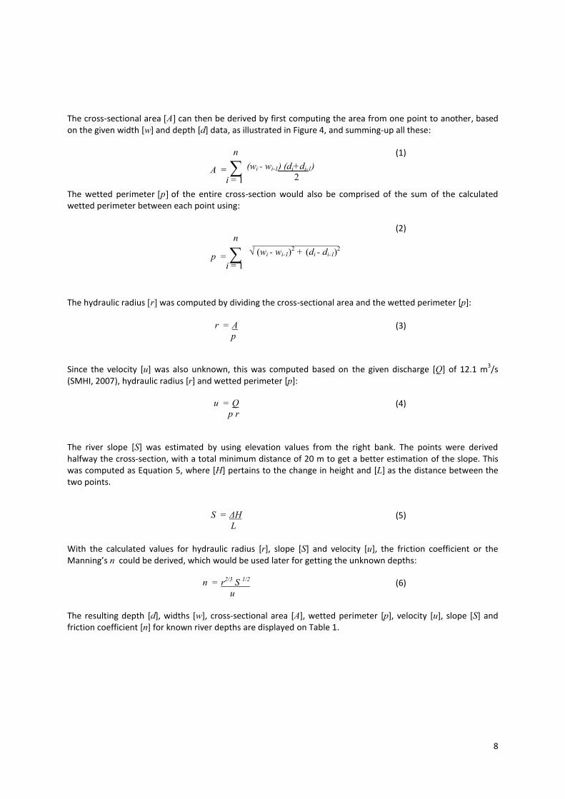
Figure 4. River’s cross-sectional area as represented by depth [d] and width [w]

d

w w0 w1 w2 w3 w4 w5 wn

d0

d2

dn

d1

d3 d5

d4

8

The cross-sectional area [A] can then be derived by first computing the area from one point to another, based on the given width [w] and depth [d] data, as illustrated in Figure 4, and summing-up all these:

A = ∑

(1)

The wetted perimeter [p] of the entire cross-section would also be comprised of the sum of the calculated wetted perimeter between each point using:

p = ∑

(2)

The hydraulic radius [r] was computed by dividing the cross-sectional area and the wetted perimeter [p]:

r = A

p (3)

Since the velocity [u] was also unknown, this was computed based on the given discharge [Q] of 12.1 m3/s

(SMHI, 2007), hydraulic radius [r] and wetted perimeter [p]:

u = Q

p r (4)

The river slope [S] was estimated by using elevation values from the right bank. The points were derived halfway the cross-section, with a total minimum distance of 20 m to get a better estimation of the slope. This was computed as Equation 5, where [H] pertains to the change in height and [L] as the distance between the two points.

S = ΔH

L (5)

With the calculated values for hydraulic radius [r], slope [S] and velocity [u], the friction coefficient or the Manning’s n could be derived, which would be used later for getting the unknown depths:

n = r2/3

S 1/2

u (6)

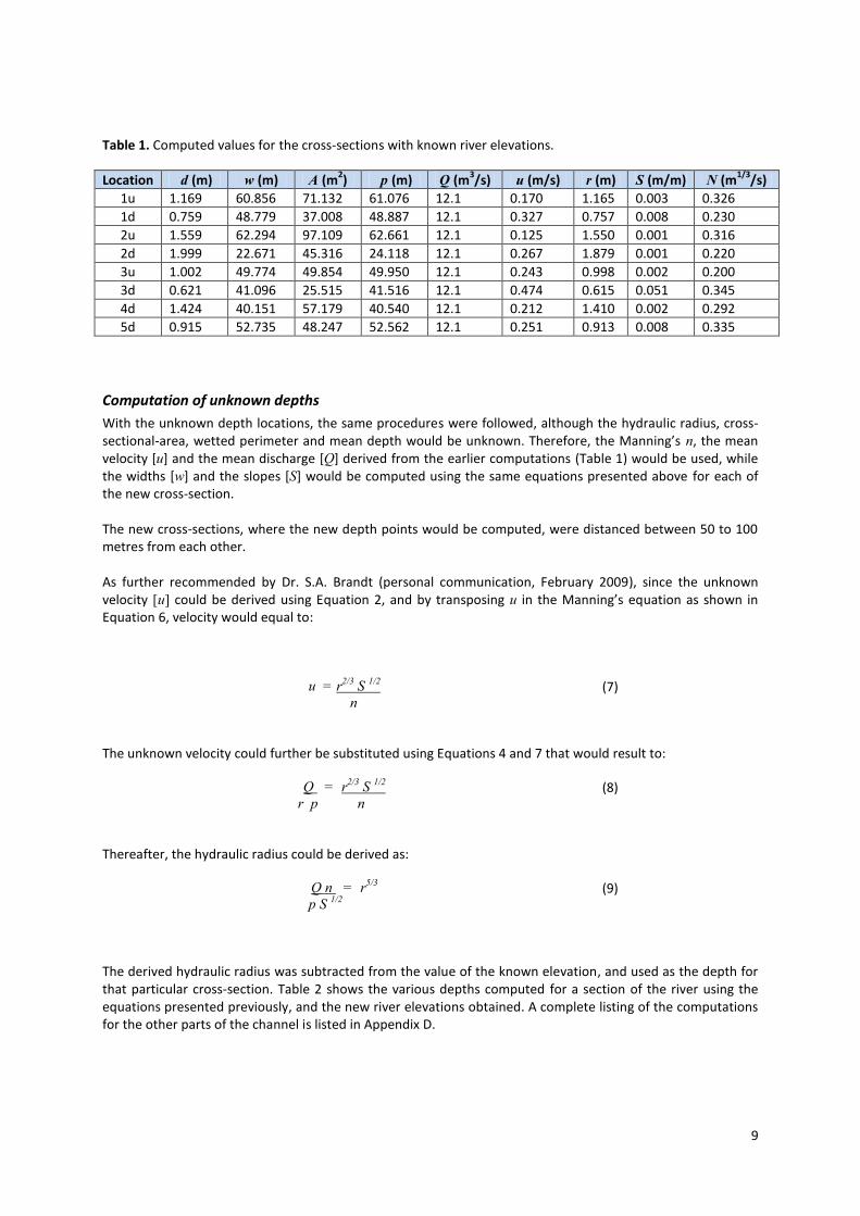
The resulting depth [d], widths [w], cross-sectional area [A], wetted perimeter [p], velocity [u], slope [S] and friction coefficient [n] for known river depths are displayed on Table 1.

n

(wi - wi-1) (di+di-1)

2 i = 1

n

√ (wi - wi-1)2 + (di - di-1)

2

i = 1

9

Table 1. Computed values for the cross-sections with known river elevations.

Location d (m) w (m) A (m2) p (m) Q (m

3/s) u (m/s) r (m) S (m/m) N (m

1/3/s)

1u 1.169 60.856 71.132 61.076 12.1 0.170 1.165 0.003 0.326

1d 0.759 48.779 37.008 48.887 12.1 0.327 0.757 0.008 0.230

2u 1.559 62.294 97.109 62.661 12.1 0.125 1.550 0.001 0.316

2d 1.999 22.671 45.316 24.118 12.1 0.267 1.879 0.001 0.220

3u 1.002 49.774 49.854 49.950 12.1 0.243 0.998 0.002 0.200

3d 0.621 41.096 25.515 41.516 12.1 0.474 0.615 0.051 0.345

4d 1.424 40.151 57.179 40.540 12.1 0.212 1.410 0.002 0.292

5d 0.915 52.735 48.247 52.562 12.1 0.251 0.913 0.008 0.335

Computation of unknown depths

With the unknown depth locations, the same procedures were followed, although the hydraulic radius, cross-sectional-area, wetted perimeter and mean depth would be unknown. Therefore, the Manning’s n, the mean velocity [u] and the mean discharge [Q] derived from the earlier computations (Table 1) would be used, while the widths [w] and the slopes [S] would be computed using the same equations presented above for each of the new cross-section. The new cross-sections, where the new depth points would be computed, were distanced between 50 to 100 metres from each other. As further recommended by Dr. S.A. Brandt (personal communication, February 2009), since the unknown velocity [u] could be derived using Equation 2, and by transposing u in the Manning’s equation as shown in Equation 6, velocity would equal to:

u = r2/3

S 1/2

n (7)

The unknown velocity could further be substituted using Equations 4 and 7 that would result to:

Q = r2/3

S 1/2

r p n (8)

Thereafter, the hydraulic radius could be derived as:

Q n = r5/3

p S 1/2

(9)

The derived hydraulic radius was subtracted from the value of the known elevation, and used as the depth for that particular cross-section. Table 2 shows the various depths computed for a section of the river using the equations presented previously, and the new river elevations obtained. A complete listing of the computations for the other parts of the channel is listed in Appendix D.

10

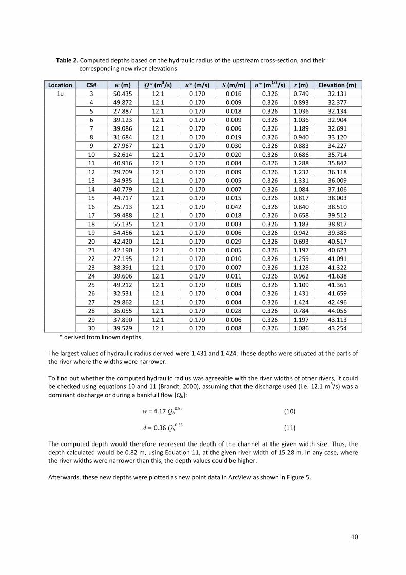
Table 2. Computed depths based on the hydraulic radius of the upstream cross-section, and their corresponding new river elevations

Location CS# w (m) Q* (m3/s) u* (m/s) S (m/m) n* (m

1/3/s) r (m) Elevation (m)

1u 3 50.435 12.1 0.170 0.016 0.326 0.749 32.131

4 49.872 12.1 0.170 0.009 0.326 0.893 32.377

5 27.887 12.1 0.170 0.018 0.326 1.036 32.134

6 39.123 12.1 0.170 0.009 0.326 1.036 32.904

7 39.086 12.1 0.170 0.006 0.326 1.189 32.691

8 31.684 12.1 0.170 0.019 0.326 0.940 33.120

9 27.967 12.1 0.170 0.030 0.326 0.883 34.227

10 52.614 12.1 0.170 0.020 0.326 0.686 35.714

11 40.916 12.1 0.170 0.004 0.326 1.288 35.842

12 29.709 12.1 0.170 0.009 0.326 1.232 36.118

13 34.935 12.1 0.170 0.005 0.326 1.331 36.009

14 40.779 12.1 0.170 0.007 0.326 1.084 37.106

15 44.717 12.1 0.170 0.015 0.326 0.817 38.003

16 25.713 12.1 0.170 0.042 0.326 0.840 38.510

17 59.488 12.1 0.170 0.018 0.326 0.658 39.512

18 55.135 12.1 0.170 0.003 0.326 1.183 38.817

19 54.456 12.1 0.170 0.006 0.326 0.942 39.388

20 42.420 12.1 0.170 0.029 0.326 0.693 40.517

21 42.190 12.1 0.170 0.005 0.326 1.197 40.623

22 27.195 12.1 0.170 0.010 0.326 1.259 41.091

23 38.391 12.1 0.170 0.007 0.326 1.128 41.322

24 39.606 12.1 0.170 0.011 0.326 0.962 41.638

25 49.212 12.1 0.170 0.005 0.326 1.109 41.361

26 32.531 12.1 0.170 0.004 0.326 1.431 41.659

27 29.862 12.1 0.170 0.004 0.326 1.424 42.496

28 35.055 12.1 0.170 0.028 0.326 0.784 44.056

29 37.890 12.1 0.170 0.006 0.326 1.197 43.113

30 39.529 12.1 0.170 0.008 0.326 1.086 43.254

* derived from known depths

The largest values of hydraulic radius derived were 1.431 and 1.424. These depths were situated at the parts of the river where the widths were narrower. To find out whether the computed hydraulic radius was agreeable with the river widths of other rivers, it could be checked using equations 10 and 11 (Brandt, 2000), assuming that the discharge used (i.e. 12.1 m

3/s) was a

dominant discharge or during a bankfull flow [Qb]:

w = 4.17 Qb0.52

(10)

d = 0.36 Qb0.33

(11)

The computed depth would therefore represent the depth of the channel at the given width size. Thus, the depth calculated would be 0.82 m, using Equation 11, at the given river width of 15.28 m. In any case, where the river widths were narrower than this, the depth values could be higher. Afterwards, these new depths were plotted as new point data in ArcView as shown in Figure 5.

11

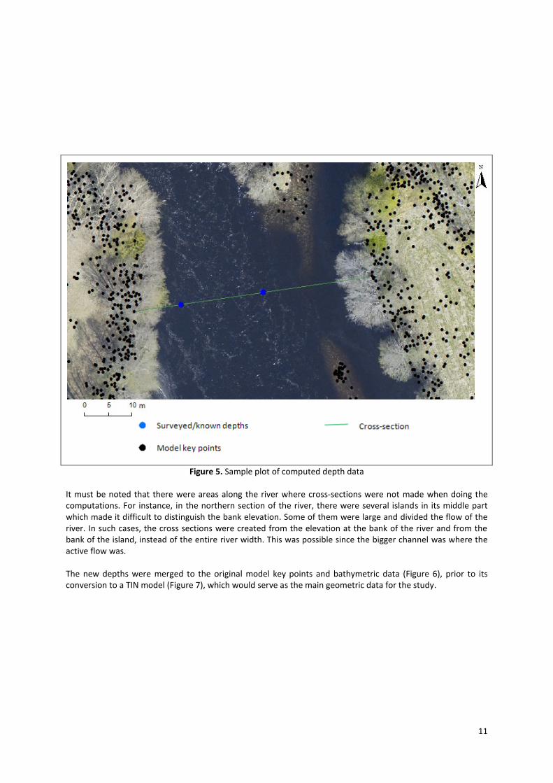
Figure 5. Sample plot of computed depth data It must be noted that there were areas along the river where cross-sections were not made when doing the computations. For instance, in the northern section of the river, there were several islands in its middle part which made it difficult to distinguish the bank elevation. Some of them were large and divided the flow of the river. In such cases, the cross sections were created from the elevation at the bank of the river and from the bank of the island, instead of the entire river width. This was possible since the bigger channel was where the active flow was. The new depths were merged to the original model key points and bathymetric data (Figure 6), prior to its conversion to a TIN model (Figure 7), which would serve as the main geometric data for the study.

12

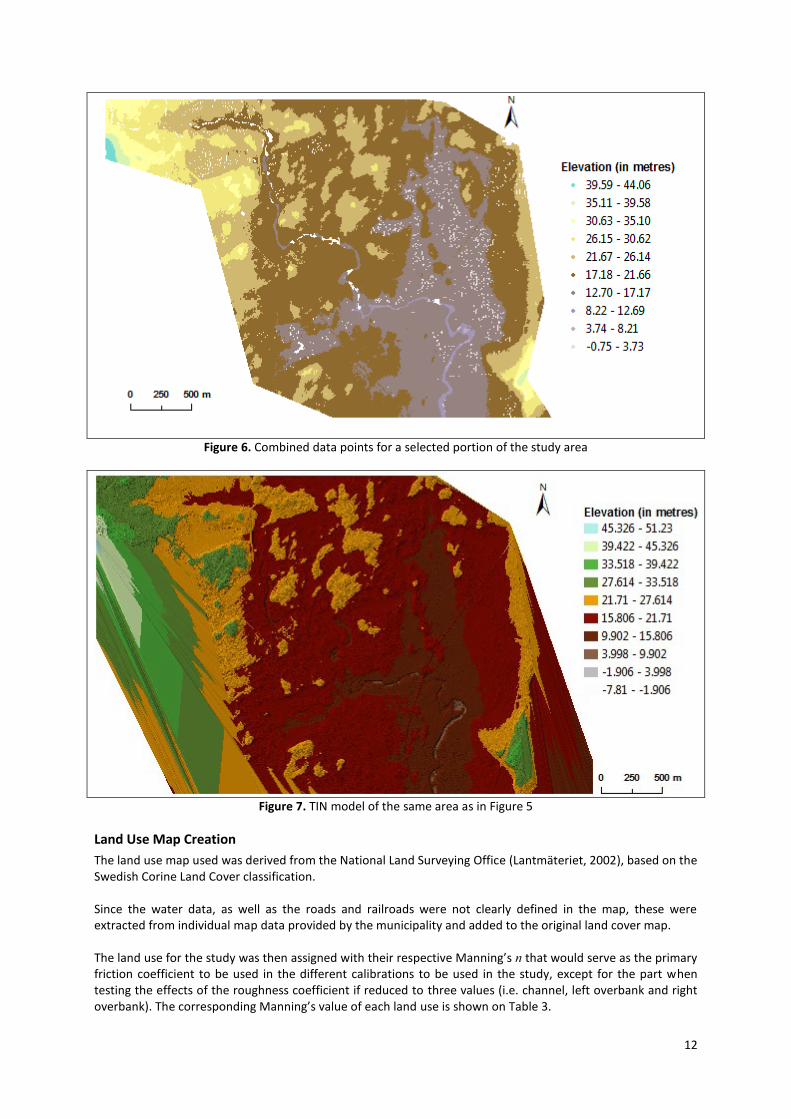
Figure 6. Combined data points for a selected portion of the study area

Figure 7. TIN model of the same area as in Figure 5

Land Use Map Creation

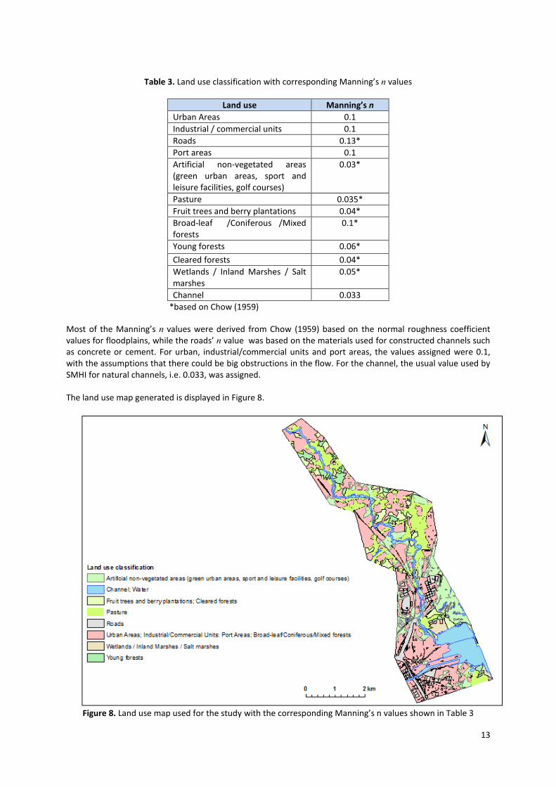
The land use map used was derived from the National Land Surveying Office (Lantmäteriet, 2002), based on the Swedish Corine Land Cover classification. Since the water data, as well as the roads and railroads were not clearly defined in the map, these were extracted from individual map data provided by the municipality and added to the original land cover map. The land use for the study was then assigned with their respective Manning’s n that would serve as the primary friction coefficient to be used in the different calibrations to be used in the study, except for the part when testing the effects of the roughness coefficient if reduced to three values (i.e. channel, left overbank and right overbank). The corresponding Manning’s value of each land use is shown on Table 3.

13

Table 3. Land use classification with corresponding Manning’s n values

Land use Manning’s n

Urban Areas 0.1

Industrial / commercial units 0.1

Roads 0.13*

Port areas 0.1

Artificial non-vegetated areas (green urban areas, sport and leisure facilities, golf courses)

0.03*

Pasture 0.035*

Fruit trees and berry plantations 0.04*

Broad-leaf /Coniferous /Mixed forests

0.1*

Young forests 0.06*

Cleared forests 0.04*

Wetlands / Inland Marshes / Salt marshes

0.05*

Channel 0.033

*based on Chow (1959)

Most of the Manning’s n values were derived from Chow (1959) based on the normal roughness coefficient values for floodplains, while the roads’ n value was based on the materials used for constructed channels such as concrete or cement. For urban, industrial/commercial units and port areas, the values assigned were 0.1, with the assumptions that there could be big obstructions in the flow. For the channel, the usual value used by SMHI for natural channels, i.e. 0.033, was assigned. The land use map generated is displayed in Figure 8.

Figure 8. Land use map used for the study with the corresponding Manning’s n values shown in Table 3

14

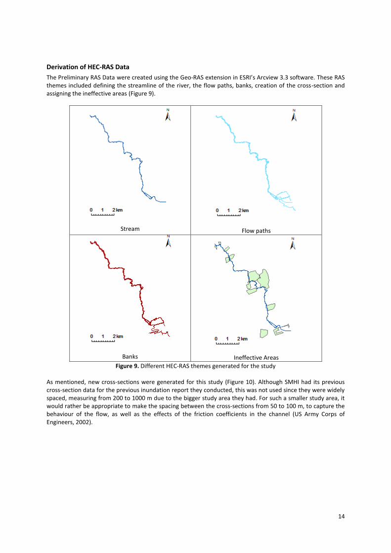
Derivation of HEC-RAS Data

The Preliminary RAS Data were created using the Geo-RAS extension in ESRI’s Arcview 3.3 software. These RAS themes included defining the streamline of the river, the flow paths, banks, creation of the cross-section and assigning the ineffective areas (Figure 9).

Stream

Flow paths

Banks

Ineffective Areas

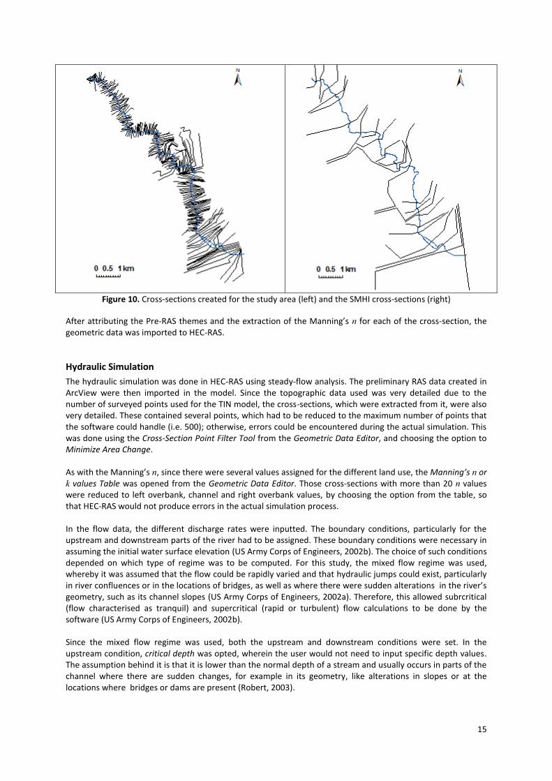
Figure 9. Different HEC-RAS themes generated for the study As mentioned, new cross-sections were generated for this study (Figure 10). Although SMHI had its previous cross-section data for the previous inundation report they conducted, this was not used since they were widely spaced, measuring from 200 to 1000 m due to the bigger study area they had. For such a smaller study area, it would rather be appropriate to make the spacing between the cross-sections from 50 to 100 m, to capture the behaviour of the flow, as well as the effects of the friction coefficients in the channel (US Army Corps of Engineers, 2002).

15

Figure 10. Cross-sections created for the study area (left) and the SMHI cross-sections (right)

After attributing the Pre-RAS themes and the extraction of the Manning’s n for each of the cross-section, the geometric data was imported to HEC-RAS.

Hydraulic Simulation

The hydraulic simulation was done in HEC-RAS using steady-flow analysis. The preliminary RAS data created in ArcView were then imported in the model. Since the topographic data used was very detailed due to the number of surveyed points used for the TIN model, the cross-sections, which were extracted from it, were also very detailed. These contained several points, which had to be reduced to the maximum number of points that the software could handle (i.e. 500); otherwise, errors could be encountered during the actual simulation. This was done using the Cross-Section Point Filter Tool from the Geometric Data Editor, and choosing the option to Minimize Area Change. As with the Manning’s n, since there were several values assigned for the different land use, the Manning’s n or k values Table was opened from the Geometric Data Editor. Those cross-sections with more than 20 n values were reduced to left overbank, channel and right overbank values, by choosing the option from the table, so that HEC-RAS would not produce errors in the actual simulation process. In the flow data, the different discharge rates were inputted. The boundary conditions, particularly for the upstream and downstream parts of the river had to be assigned. These boundary conditions were necessary in assuming the initial water surface elevation (US Army Corps of Engineers, 2002b). The choice of such conditions depended on which type of regime was to be computed. For this study, the mixed flow regime was used, whereby it was assumed that the flow could be rapidly varied and that hydraulic jumps could exist, particularly in river confluences or in the locations of bridges, as well as where there were sudden alterations in the river’s geometry, such as its channel slopes (US Army Corps of Engineers, 2002a). Therefore, this allowed subrcritical (flow characterised as tranquil) and supercritical (rapid or turbulent) flow calculations to be done by the software (US Army Corps of Engineers, 2002b). Since the mixed flow regime was used, both the upstream and downstream conditions were set. In the upstream condition, critical depth was opted, wherein the user would not need to input specific depth values. The assumption behind it is that it is lower than the normal depth of a stream and usually occurs in parts of the channel where there are sudden changes, for example in its geometry, like alterations in slopes or at the locations where bridges or dams are present (Robert, 2003).

16

For the downstream condition, a known water surface elevation (i.e. 1.598 m a.s.l.) was specified to be its boundary condition. This value was converted based on its original value derived from SMHI (2002), which was 1.4 m using the height system of RH70. To convert to the same height reference system that was used for the study (i.e. RH 2000), this was added with 0.918, based on the conversion factor of the two height systems (Gävle Kommun, 2006).

Flood Delineation

After the simulation was done, the HEC-RAS results were exported to GIS data as Post-RAS themes prior to opening them in ArcView. In ArcView, the floodplain was delineated using raster cell size of 0.50 metres to give better resolution to the water surfaces.

Calibration

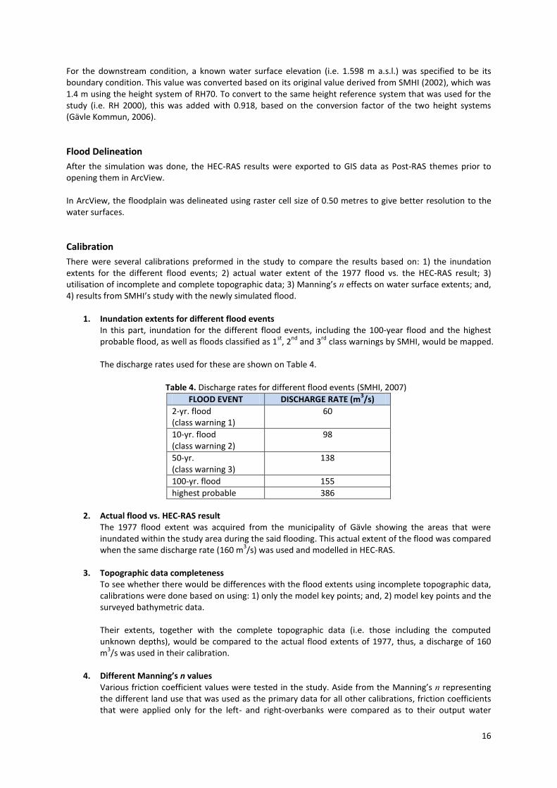
There were several calibrations preformed in the study to compare the results based on: 1) the inundation extents for the different flood events; 2) actual water extent of the 1977 flood vs. the HEC-RAS result; 3) utilisation of incomplete and complete topographic data; 3) Manning’s n effects on water surface extents; and, 4) results from SMHI’s study with the newly simulated flood.

1. Inundation extents for different flood events In this part, inundation for the different flood events, including the 100-year flood and the highest probable flood, as well as floods classified as 1

st, 2

nd and 3

rd class warnings by SMHI, would be mapped.

The discharge rates used for these are shown on Table 4. Table 4. Discharge rates for different flood events (SMHI, 2007)

FLOOD EVENT DISCHARGE RATE (m3/s)

2-yr. flood (class warning 1)

60

10-yr. flood (class warning 2)

98

50-yr. (class warning 3)

138

100-yr. flood 155

highest probable 386

2. Actual flood vs. HEC-RAS result The 1977 flood extent was acquired from the municipality of Gävle showing the areas that were inundated within the study area during the said flooding. This actual extent of the flood was compared when the same discharge rate (160 m

3/s) was used and modelled in HEC-RAS.

3. Topographic data completeness

To see whether there would be differences with the flood extents using incomplete topographic data, calibrations were done based on using: 1) only the model key points; and, 2) model key points and the surveyed bathymetric data. Their extents, together with the complete topographic data (i.e. those including the computed unknown depths), would be compared to the actual flood extents of 1977, thus, a discharge of 160 m

3/s was used in their calibration.

4. Different Manning’s n values

Various friction coefficient values were tested in the study. Aside from the Manning’s n representing the different land use that was used as the primary data for all other calibrations, friction coefficients that were applied only for the left- and right-overbanks were compared as to their output water

17

extents. These values were 0.025, 0.05, 0.10 and 0.20 (Brandt, 2009). The channel’s n value was fixed to 0.033 for the entire study.

5. SMHI inundation results vs. the newly simulated study As mentioned earlier, SMHI conducted an inundation modelling in 2002. For the 100-yr flood, the discharge used was 165 m

3/s. Although Mike-11 software was used for the simulation, as well as

different topographic and cross-sectional data, their results would be compared to the simulated result of HEC-RAS using the same water discharge.

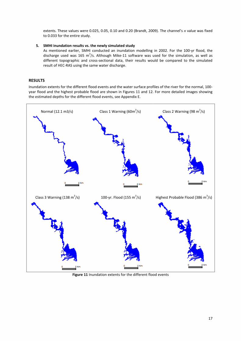
RESULTS

Inundation extents for the different flood events and the water surface profiles of the river for the normal, 100-year flood and the highest probable flood are shown in Figures 11 and 12. For more detailed images showing the estimated depths for the different flood events, see Appendix E.

Normal (12.1 m3/s)

Class 1 Warning (60m

3/s)

Class 2 Warning (98 m

3/s)

Class 3 Warning (138 m

3/s)

100-yr. Flood (155 m

3/s)

Highest Probable Flood (386 m

3/s)

Figure 11 Inundation extents for the different flood events

18

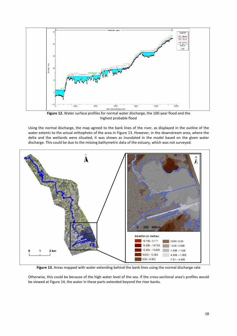
Figure 12. Water surface profiles for normal water discharge, the 100-year flood and the

highest probable flood

Using the normal discharge, the map agreed to the bank lines of the river, as displayed in the outline of the water extents to the actual orthophoto of the area in Figure 13. However, in the downstream area, where the delta and the wetlands were situated, it was shown as inundated in the model based on the given water discharge. This could be due to the missing bathymetric data of the estuary, which was not surveyed.

Figure 13. Areas mapped with water extending behind the bank lines using the normal discharge rate

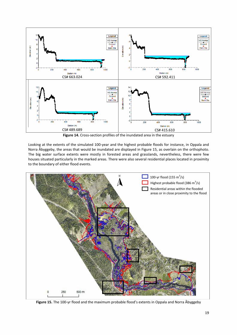
Otherwise, this could be because of the high water level of the sea. If the cross-sectional area’s profiles would be viewed at Figure 14, the water in these parts extended beyond the river banks.

19

Highest probable flood (386 m3/s)

100-yr flood (155 m3/s)

Residential areas within the flooded areas or in close proximity to the flood

CS# 663.024 CS# 592.411

CS# 489.689 CS# 415.610

Figure 14. Cross-section profiles of the inundated area in the estuary

Looking at the extents of the simulated 100-year and the highest probable floods for instance, in Oppala and Norra Åbyggeby, the areas that would be inundated are displayed in Figure 15, as overlain on the orthophoto. The big water surface extents were mostly in forested areas and grasslands, nevertheless, there were few houses situated particularly in the marked areas. There were also several residential places located in proximity to the boundary of either flood events.

Figure 15. The 100-yr flood and the maximum probable flood’s extents in Oppala and Norra Åbyggeby

20

Highest probable flood (386 m3/s)

100-yr flood (155 m3/s)

Residential areas within the flooded areas or in close proximity to the flood

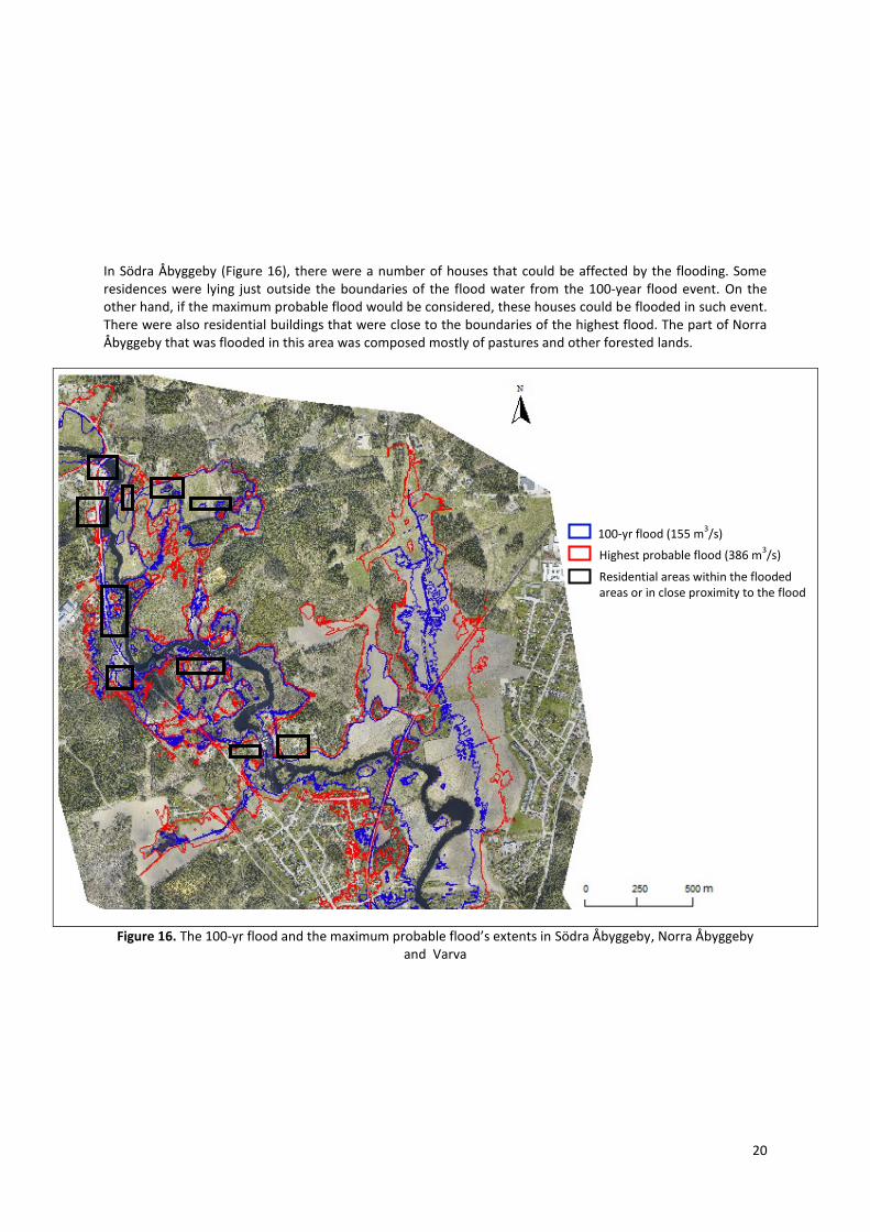
In Södra Åbyggeby (Figure 16), there were a number of houses that could be affected by the flooding. Some residences were lying just outside the boundaries of the flood water from the 100-year flood event. On the other hand, if the maximum probable flood would be considered, these houses could be flooded in such event. There were also residential buildings that were close to the boundaries of the highest flood. The part of Norra Åbyggeby that was flooded in this area was composed mostly of pastures and other forested lands.

Figure 16. The 100-yr flood and the maximum probable flood’s extents in Södra Åbyggeby, Norra Åbyggeby and Varva

21

Highest probable flood (386 m3/s)

100-yr flood (155 m3/s) Residential areas within the flooded

areas or in close proximity to the flood

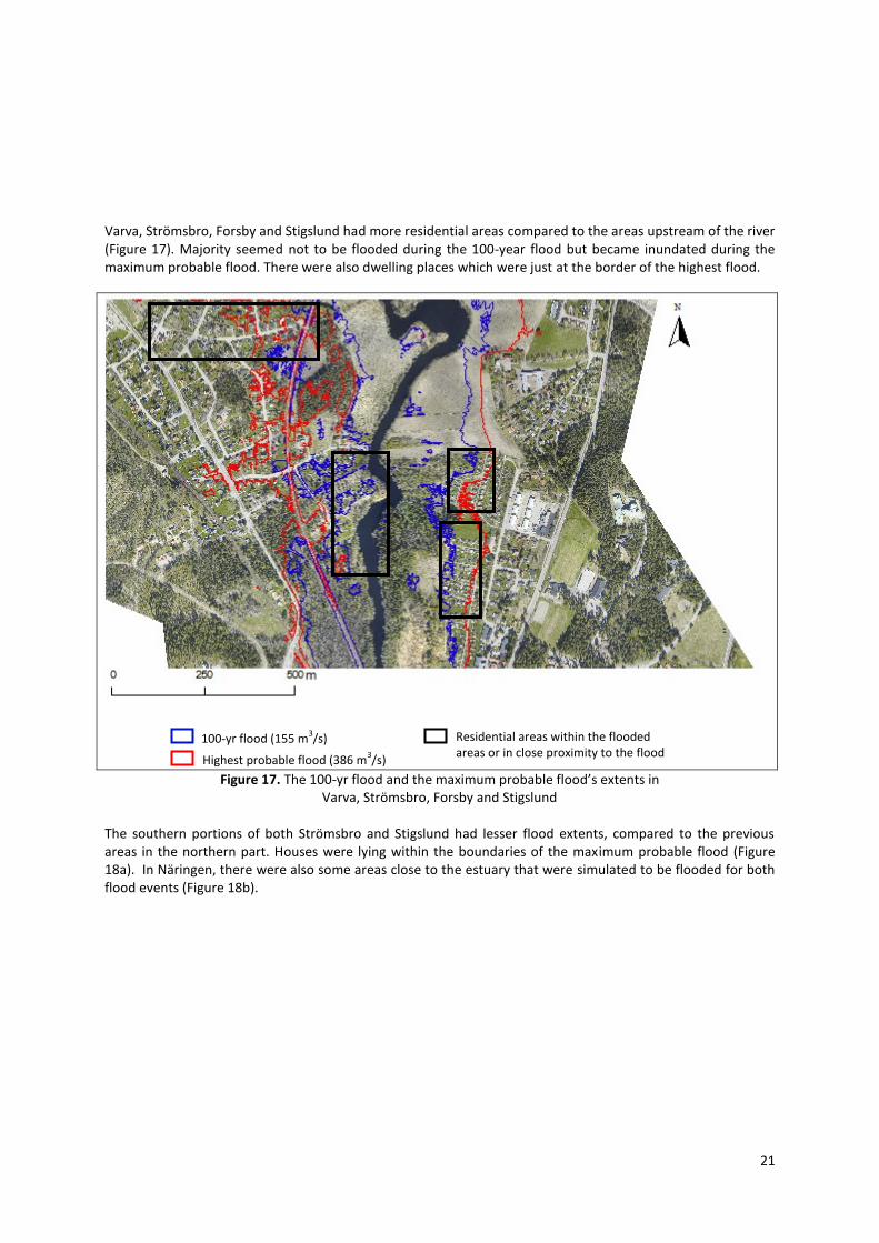
Varva, Strömsbro, Forsby and Stigslund had more residential areas compared to the areas upstream of the river (Figure 17). Majority seemed not to be flooded during the 100-year flood but became inundated during the maximum probable flood. There were also dwelling places which were just at the border of the highest flood.

Figure 17. The 100-yr flood and the maximum probable flood’s extents in Varva, Strömsbro, Forsby and Stigslund

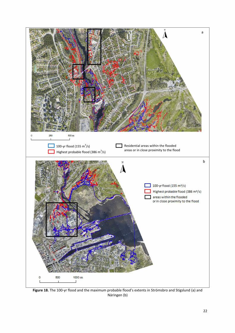
The southern portions of both Strömsbro and Stigslund had lesser flood extents, compared to the previous areas in the northern part. Houses were lying within the boundaries of the maximum probable flood (Figure 18a). In Näringen, there were also some areas close to the estuary that were simulated to be flooded for both flood events (Figure 18b).

22

Figure 18. The 100-yr flood and the maximum probable flood’s extents in Strömsbro and Stigslund (a) and

Näringen (b)

Highest probable flood (386 m3/s)

100-yr flood (155 m3/s) Residential areas within the flooded

areas or in close proximity to the flood

a

b

23

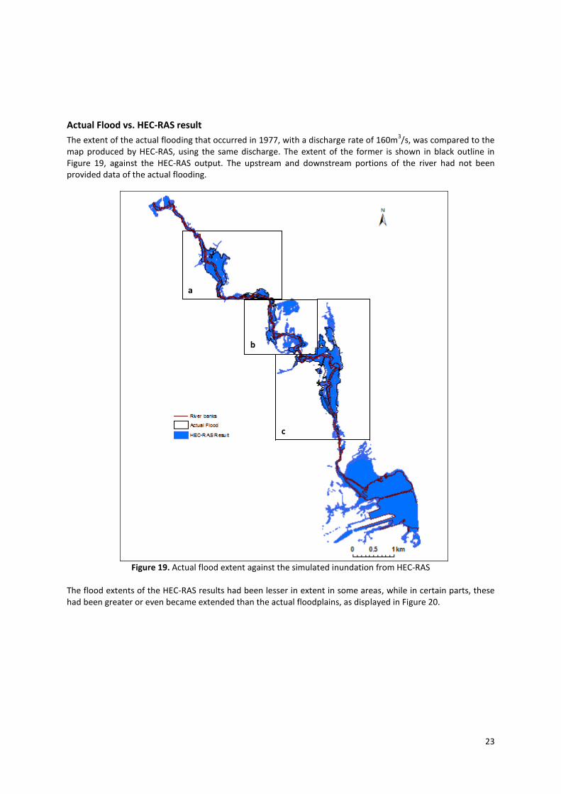
Actual Flood vs. HEC-RAS result

The extent of the actual flooding that occurred in 1977, with a discharge rate of 160m3/s, was compared to the

map produced by HEC-RAS, using the same discharge. The extent of the former is shown in black outline in Figure 19, against the HEC-RAS output. The upstream and downstream portions of the river had not been provided data of the actual flooding.

Figure 19. Actual flood extent against the simulated inundation from HEC-RAS

The flood extents of the HEC-RAS results had been lesser in extent in some areas, while in certain parts, these had been greater or even became extended than the actual floodplains, as displayed in Figure 20.

a

b

c

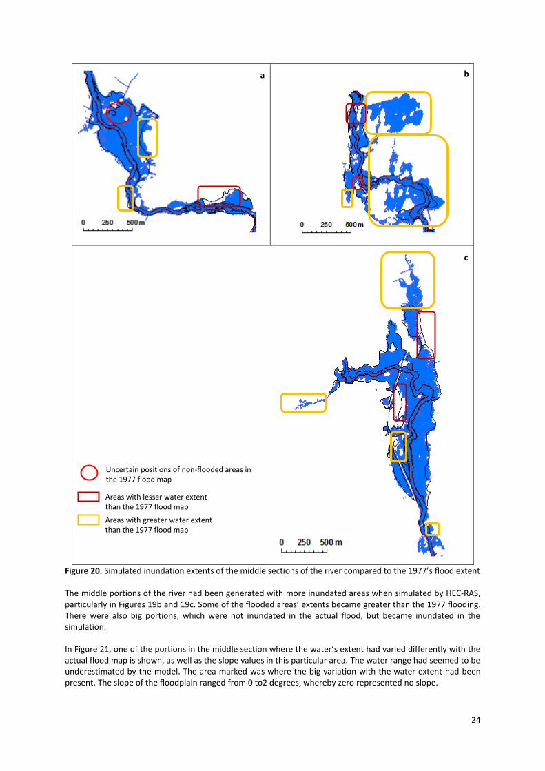
24

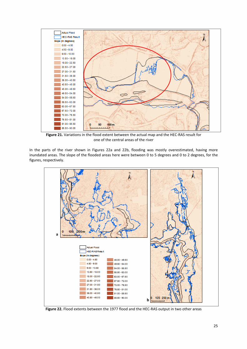
Figure 20. Simulated inundation extents of the middle sections of the river compared to the 1977’s flood extent The middle portions of the river had been generated with more inundated areas when simulated by HEC-RAS, particularly in Figures 19b and 19c. Some of the flooded areas’ extents became greater than the 1977 flooding. There were also big portions, which were not inundated in the actual flood, but became inundated in the simulation. In Figure 21, one of the portions in the middle section where the water’s extent had varied differently with the actual flood map is shown, as well as the slope values in this particular area. The water range had seemed to be underestimated by the model. The area marked was where the big variation with the water extent had been present. The slope of the floodplain ranged from 0 to2 degrees, whereby zero represented no slope.

a b

c

Areas with lesser water extent than the 1977 flood map

Areas with greater water extent than the 1977 flood map

Uncertain positions of non-flooded areas in the 1977 flood map

25

Figure 21. Variations in the flood extent between the actual map and the HEC-RAS result for

one of the central areas of the river In the parts of the river shown in Figures 22a and 22b, flooding was mostly overestimated, having more inundated areas. The slope of the flooded areas here were between 0 to 5 degrees and 0 to 2 degrees, for the figures, respectively.

Figure 22. Flood extents between the 1977 flood and the HEC-RAS output in two other areas

a

b

26

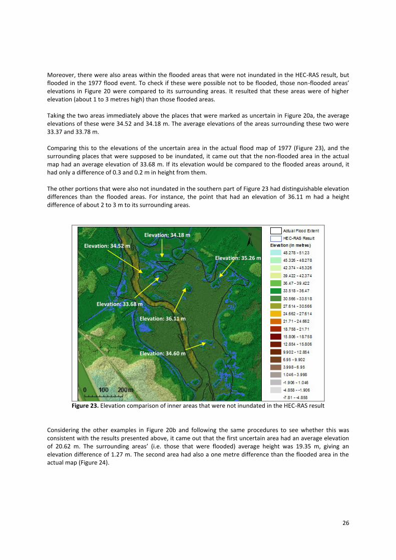
Moreover, there were also areas within the flooded areas that were not inundated in the HEC-RAS result, but flooded in the 1977 flood event. To check if these were possible not to be flooded, those non-flooded areas’ elevations in Figure 20 were compared to its surrounding areas. It resulted that these areas were of higher elevation (about 1 to 3 metres high) than those flooded areas. Taking the two areas immediately above the places that were marked as uncertain in Figure 20a, the average elevations of these were 34.52 and 34.18 m. The average elevations of the areas surrounding these two were 33.37 and 33.78 m. Comparing this to the elevations of the uncertain area in the actual flood map of 1977 (Figure 23), and the surrounding places that were supposed to be inundated, it came out that the non-flooded area in the actual map had an average elevation of 33.68 m. If its elevation would be compared to the flooded areas around, it had only a difference of 0.3 and 0.2 m in height from them. The other portions that were also not inundated in the southern part of Figure 23 had distinguishable elevation differences than the flooded areas. For instance, the point that had an elevation of 36.11 m had a height difference of about 2 to 3 m to its surrounding areas.

Figure 23. Elevation comparison of inner areas that were not inundated in the HEC-RAS result

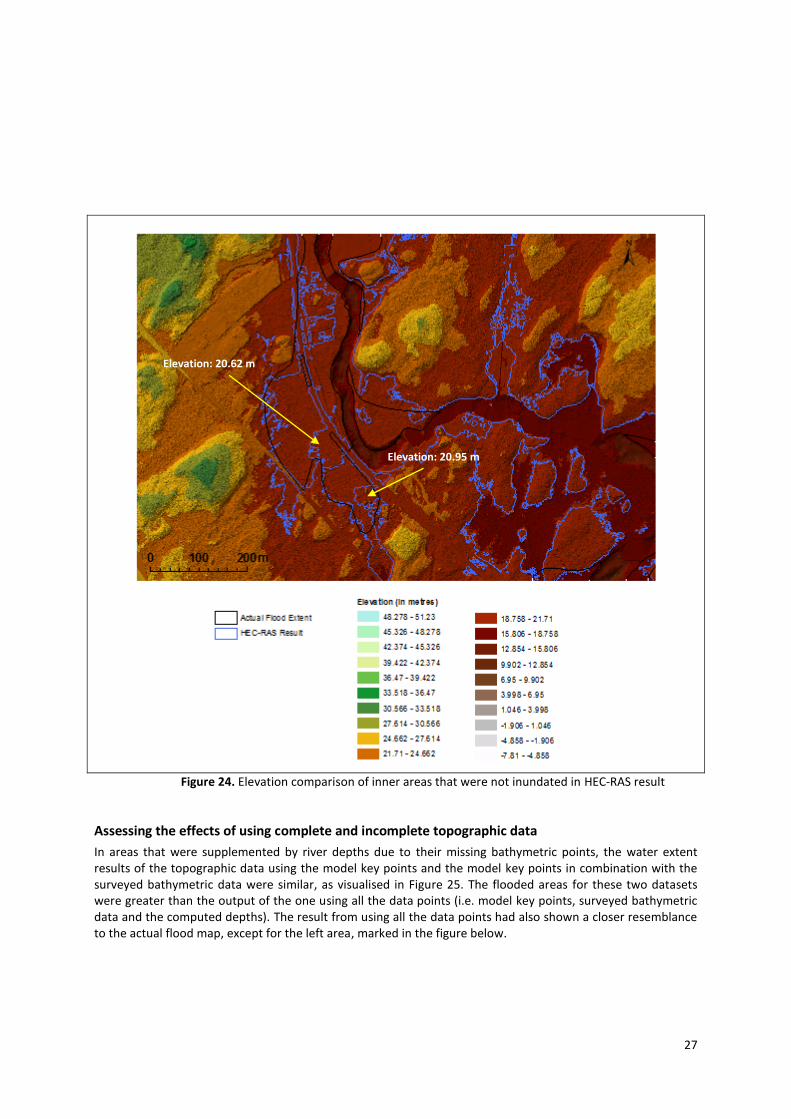
Considering the other examples in Figure 20b and following the same procedures to see whether this was consistent with the results presented above, it came out that the first uncertain area had an average elevation of 20.62 m. The surrounding areas’ (i.e. those that were flooded) average height was 19.35 m, giving an elevation difference of 1.27 m. The second area had also a one metre difference than the flooded area in the actual map (Figure 24).

Elevation: 34.52 m

Elevation: 34.18 m

Elevation: 33.68 m

Elevation: 36.11 m

Elevation: 35.26 m

Elevation: 34.60 m

27

Figure 24. Elevation comparison of inner areas that were not inundated in HEC-RAS result

Assessing the effects of using complete and incomplete topographic data

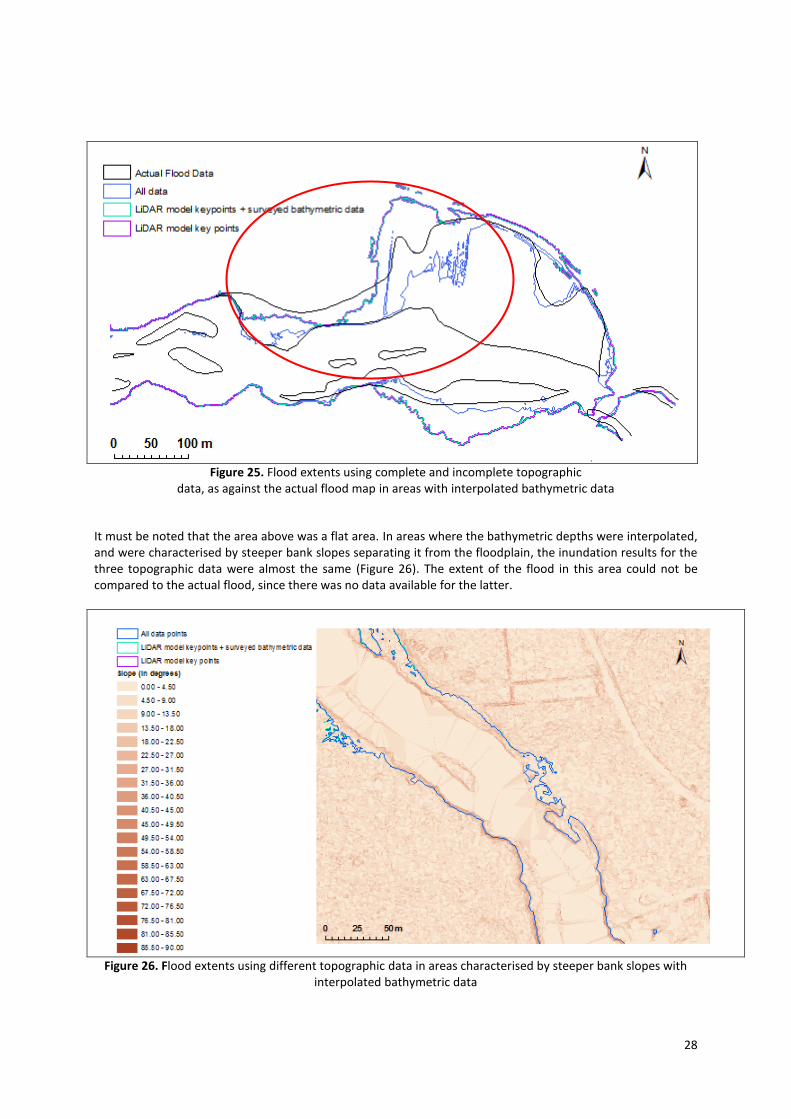
In areas that were supplemented by river depths due to their missing bathymetric points, the water extent results of the topographic data using the model key points and the model key points in combination with the surveyed bathymetric data were similar, as visualised in Figure 25. The flooded areas for these two datasets were greater than the output of the one using all the data points (i.e. model key points, surveyed bathymetric data and the computed depths). The result from using all the data points had also shown a closer resemblance to the actual flood map, except for the left area, marked in the figure below.

Elevation: 20.62 m

Elevation: 20.95 m

28

Figure 25. Flood extents using complete and incomplete topographic

data, as against the actual flood map in areas with interpolated bathymetric data

It must be noted that the area above was a flat area. In areas where the bathymetric depths were interpolated, and were characterised by steeper bank slopes separating it from the floodplain, the inundation results for the three topographic data were almost the same (Figure 26). The extent of the flood in this area could not be compared to the actual flood, since there was no data available for the latter.

Figure 26. Flood extents using different topographic data in areas characterised by steeper bank slopes with

interpolated bathymetric data

29

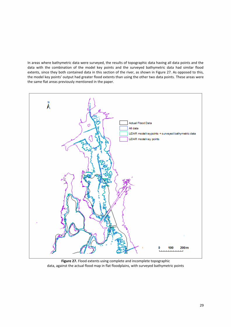
In areas where bathymetric data were surveyed, the results of topographic data having all data points and the data with the combination of the model key points and the surveyed bathymetric data had similar flood extents, since they both contained data in this section of the river, as shown in Figure 27. As opposed to this, the model key points’ output had greater flood extents than using the other two data points. These areas were the same flat areas previously mentioned in the paper.

Figure 27. Flood extents using complete and incomplete topographic data, against the actual flood map in flat floodplains, with surveyed bathymetric points

30

Calibration of different Manning’s n values for the left- and right overbanks

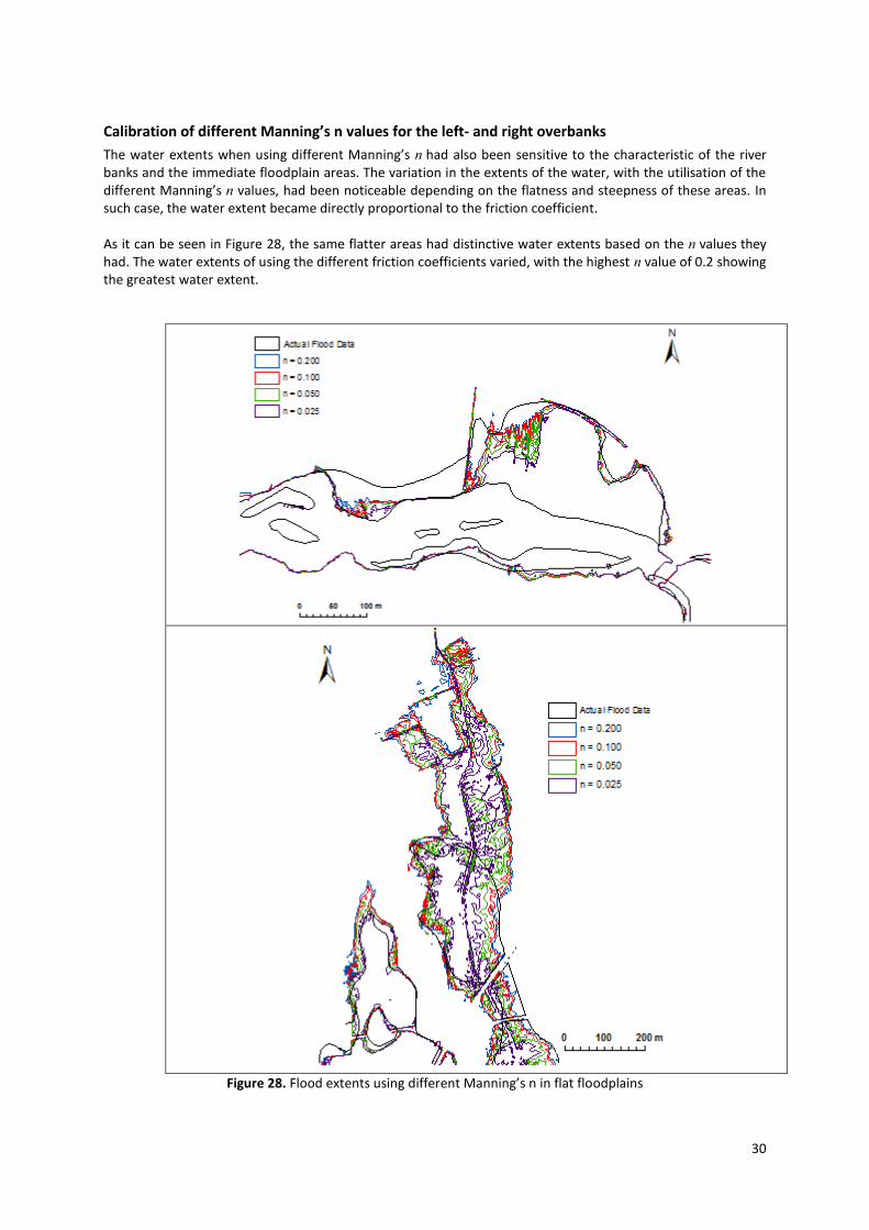
The water extents when using different Manning’s n had also been sensitive to the characteristic of the river banks and the immediate floodplain areas. The variation in the extents of the water, with the utilisation of the different Manning’s n values, had been noticeable depending on the flatness and steepness of these areas. In such case, the water extent became directly proportional to the friction coefficient. As it can be seen in Figure 28, the same flatter areas had distinctive water extents based on the n values they had. The water extents of using the different friction coefficients varied, with the highest n value of 0.2 showing the greatest water extent.

Figure 28. Flood extents using different Manning’s n in flat floodplains

31

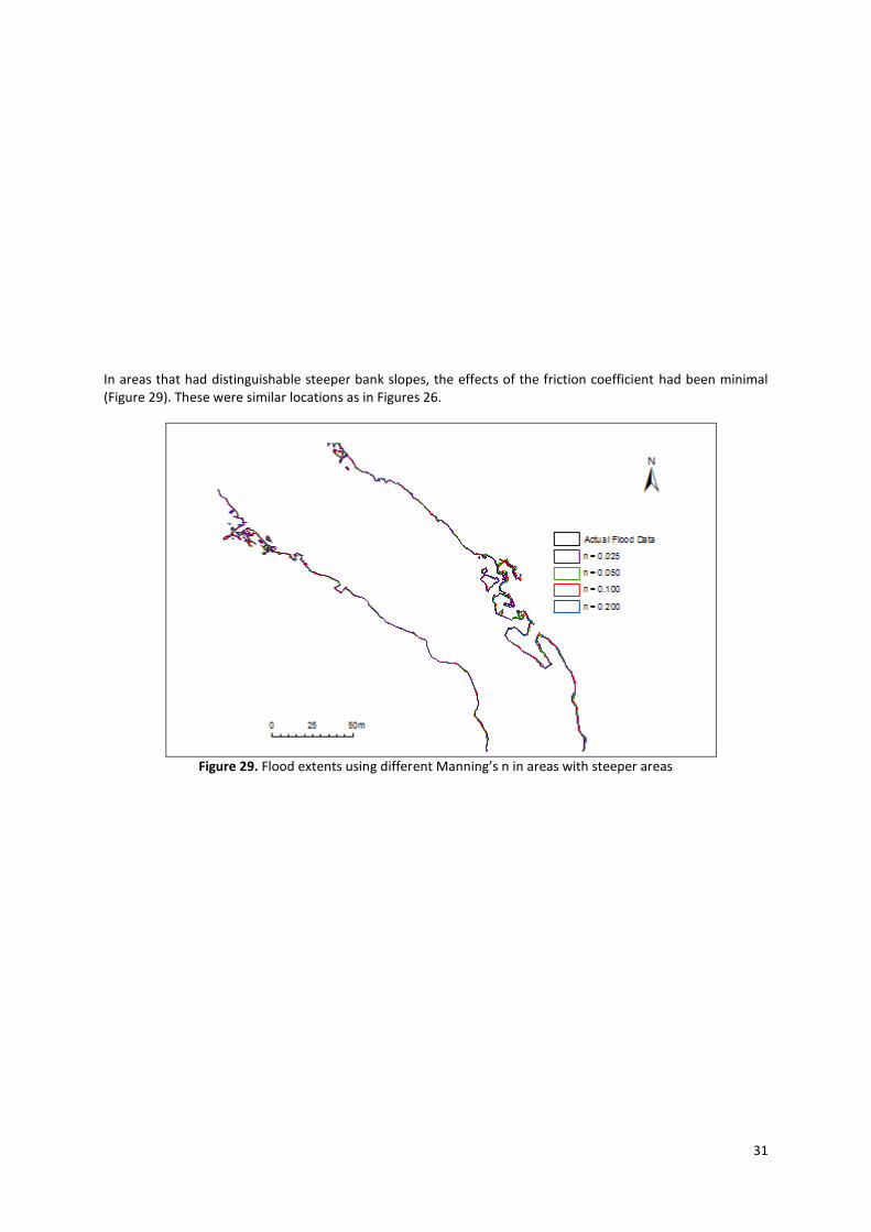
In areas that had distinguishable steeper bank slopes, the effects of the friction coefficient had been minimal (Figure 29). These were similar locations as in Figures 26.

Figure 29. Flood extents using different Manning’s n in areas with steeper areas

32

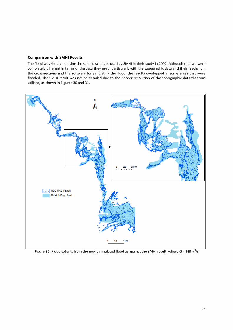
Comparison with SMHI Results

The flood was simulated using the same discharges used by SMHI in their study in 2002. Although the two were completely different in terms of the data they used, particularly with the topographic data and their resolution, the cross-sections and the software for simulating the flood, the results overlapped in some areas that were flooded. The SMHI result was not so detailed due to the poorer resolution of the topographic data that was utilised, as shown in Figures 30 and 31.

Figure 30. Flood extents from the newly simulated flood as against the SMHI result, where Q = 165 m3/s

33

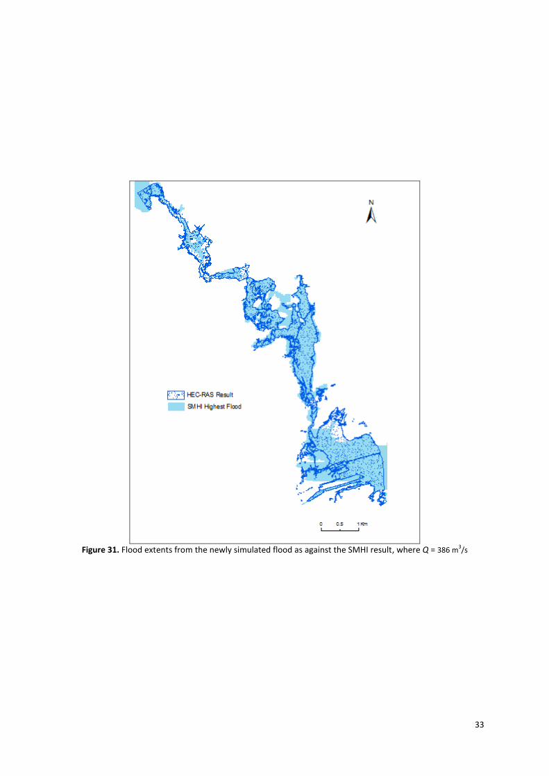
Figure 31. Flood extents from the newly simulated flood as against the SMHI result, where Q = 386 m3/s

34

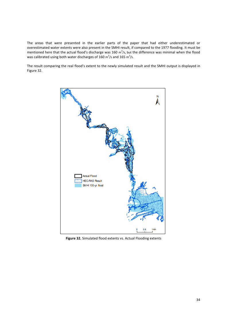
The areas that were presented in the earlier parts of the paper that had either underestimated or overestimated water extents were also present in the SMHI result, if compared to the 1977 flooding. It must be mentioned here that the actual flood’s discharge was 160 m3

/s, but the difference was minimal when the flood was calibrated using both water discharges of 160 m3

/s and 165 m3/s.

The result comparing the real flood’s extent to the newly simulated result and the SMHI output is displayed in Figure 32.

Figure 32. Simulated flood extents vs. Actual Flooding extents

35

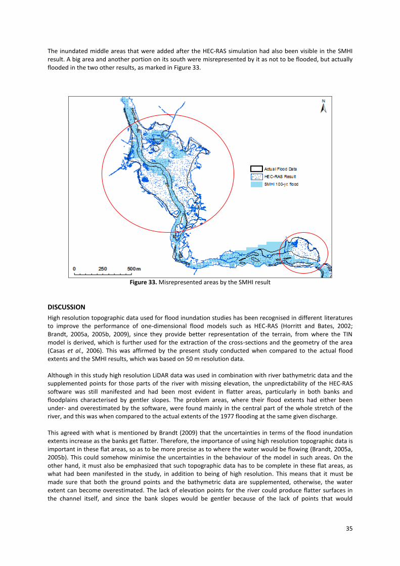
The inundated middle areas that were added after the HEC-RAS simulation had also been visible in the SMHI result. A big area and another portion on its south were misrepresented by it as not to be flooded, but actually flooded in the two other results, as marked in Figure 33.

Figure 33. Misrepresented areas by the SMHI result

DISCUSSION

High resolution topographic data used for flood inundation studies has been recognised in different literatures to improve the performance of one-dimensional flood models such as HEC-RAS (Horritt and Bates, 2002; Brandt, 2005a, 2005b, 2009), since they provide better representation of the terrain, from where the TIN model is derived, which is further used for the extraction of the cross-sections and the geometry of the area (Casas et al., 2006). This was affirmed by the present study conducted when compared to the actual flood extents and the SMHI results, which was based on 50 m resolution data. Although in this study high resolution LiDAR data was used in combination with river bathymetric data and the supplemented points for those parts of the river with missing elevation, the unpredictability of the HEC-RAS software was still manifested and had been most evident in flatter areas, particularly in both banks and floodplains characterised by gentler slopes. The problem areas, where their flood extents had either been under- and overestimated by the software, were found mainly in the central part of the whole stretch of the river, and this was when compared to the actual extents of the 1977 flooding at the same given discharge. This agreed with what is mentioned by Brandt (2009) that the uncertainties in terms of the flood inundation extents increase as the banks get flatter. Therefore, the importance of using high resolution topographic data is important in these flat areas, so as to be more precise as to where the water would be flowing (Brandt, 2005a, 2005b). This could somehow minimise the uncertainties in the behaviour of the model in such areas. On the other hand, it must also be emphasized that such topographic data has to be complete in these flat areas, as what had been manifested in the study, in addition to being of high resolution. This means that it must be made sure that both the ground points and the bathymetric data are supplemented, otherwise, the water extent can become overestimated. The lack of elevation points for the river could produce flatter surfaces in the channel itself, and since the bank slopes would be gentler because of the lack of points that would

36

distinguish the river elevation from the floodplain’s elevation, the water surface gets broader. As a result of the flatness of the floodplain, the water could flow freely to these areas when the river overflows. Resolution and completeness of data were not the only problems that could impact the water surface levels in flatter areas. These complications could further be affected by the values of the Manning’s coefficient. The variations of the water surface extents were noticeable with different n values, particularly with higher roughness coefficient causing greater extents in these areas. Nevertheless in places characterised by steeper slopes bounding the channel from the floodplain, or in the areas within the floodplain confined by a steeper slope, which limited the water from overflowing, their effects had been minimal. Therefore, the importance of using the correct Manning’s n value would be of significance in flatter locations, as what was cited by Brandt (2005a, 2005b). On the contrary, this would also mean the inappropriateness of using only a single overbank n value, in addition to the channel’s friction coefficient, since in reality, the Manning’s n is heterogeneous (Schumann et al., 2008), depending on the characteristics of the floodplain’s surface. Thus, this would lead to other questions such as how to estimate the Manning’s n for this area, especially for a huge floodplain, and how accurate the values should be. Moreover, HEC-RAS has also its limitation of handling too many Manning’s n values. The software could only process a maximum of 20 roughness coefficients for every cross-section. Otherwise, the user has to cut down the values based on the maximum allowable n values or to reduce it to the channel, and its right- and left overbanks Manning’s n. Therefore, too detailed roughness coefficient in the floodplain could also be irrelevant. Parameterisation problems such as this has been attributed to be the cause of uncertainties specifically of HEC-RAS (Horritt and Bates, 2002; Hicks and Peacock, 2005; Pappenberger et al., 2005). Yet, in this study, the basis of the accurateness of the HEC-RAS results was based in comparing it to the map of the actual flood that happened in 1977. At some point, the reliability of how this was derived and created became a concern. In most of the inner areas modelled by HEC-RAS as non-flooded, the elevation difference between this location and the surrounding areas had been distinctively different, with differences of up to 1 m. Therefore, the accurateness of the actual flood extents could also be misleading. Thus, the question would be which among these represented the real flood extents. It must be remembered that the actual extent of the flooding could also vary with time. The floodplain can be affected by changes, particularly of land use. What particular usage the land had for more than 30 years ago could be different at present. They could have been converted, for instance, from forests to farmland. This could have been the case for where the actual flood extent had. The land use data that was used for the simulation was based on the Corine Landuse Classification as of 2003, and thus, it could not be certain whether the same land use was applicable when the flooding occurred. And since the land use is the basis for the Manning’s n, and if its values and their differentiation are significant in inundation studies, as what was mentioned by Brandt (2005a), Manning’s n become time dependent if calibrated with real-life flood surface levels. Therefore, time is also a factor to be considered with inundation studies. An appropriate inundation study today could never be guaranteed with the same results five to ten years from now, due to the changes that are happening to the topography of the area, either instigated by man or by nature. Therefore, if inundation studies would be used in planning, it must consider such changes that are continuously happening. In addition, if the HEC-RAS output would be compared to the created maps of SMHI, the new simulation had provided better inundation results even when both were compared to the extents of the 1977 flooding. The big part that was not inundated in SMHI’s simulation of the 100-year flood but was supposed to be flooded during the actual event showed the inappropriateness of the map it produced in providing water surface profiles that could be utilised for planning. This could lead to risky decisions that could put lives and properties in danger. Consequently, this brings to a bigger question as to the reliability of all inundation maps for the different rivers in the country that to date have been produced for the Swedish Rescue Agency. If these maps would continuously be used by the agency or any municipality to arrive at emergency plans in case of great floods, safety of the population could be compromised. Finally, in the inundation extents resulted by the model, it could be noticed that majority of the residential areas in the populated places such as Strömsbro, Varva, Stigslund and Forsby were outside the 100-year flood’s extent, but were inundated with the highest flood. In spite of these results, it must be noted that the discharge used for this was based on the data as of June 2007. This could change as new maximum discharge is recorded

37

or when an extreme weather condition suddenly occurs, which could be possible due to the effects of climate change. Thereupon, these two should be regarded during the actual planning process. In Norra Åbyggeby, where the flat areas were common and where the software had manifested its sensitivity, careful consideration must be made if houses or other establishments are to be built here. Due to its terrain characteristics, the flood behaviour could be difficult to model, as well as the flow of water that may lead to miscalculations as to where the water would be.

CONCLUSION

Different flooding events were simulated using the HEC-RAS steady flow simulation software for Testeboån. However, the central part of the river that was characterised by flatter floodplains and gentler bank slopes had drawn attention in terms of the output produced by the model after several simulations. Although high resolution and complete data were used, flood extents in these sites could not be calibrated to get the desired inundation result if compared with the actual flood event of 1977. The area had also manifested sensitivity to the values of Manning’s n, particularly when values were limited only to the main channel, and the left- and right-overbanks of the river. Therefore, caution must be particularly made in these particular locations, since the behaviour of the water flow was unpredictable. Flooding can either be over- or underestimated. This does not mean that inundation studies can never accurately predict floods. The reason may be attributed to the fact that the behaviour of actual floods are difficult to determine. The different models used for simulating them have their own assumptions and limitations, in addition to data constraints. Thus, knowing these problems with the unpredictability of how much water there would be, or how high and up to what extent the flood could reach, it would rather be appropriate to overestimate a future flood’s behaviour rather than underestimate it. Although most of the inundations studies rely on statistical data such as the flood extents of the 100-year flood, it must be noted that statistical data such as this can also change from year to year, as new statistical data are acquired.

REFERENCES

Bates, P.D. and De Roo, A.P. (2000) ’A simple raster-based model for flood inundation simulation’, Journal of Hydrology, 236 (1-2), pp. 54-77. Bonde, L., and Ståhl, P. (1995) Värdefull natur i Gävle. Gävle: Miljökontoret. Brandt, S.A. (2000) ’Prediction of Downstream Geomorphological Changes after Dam Construction: A Stream Power Approach’, Water Resources and Development, 16 (3), pp. 343-367. Brandt, S.A. (2005a) ’Resolution issues of elevation during inundation modeling of river floods’, XXX1 International Association of Hydraulic Engineering and Research Congress, Water Engineering for the Future: Choices and Challenges. Seoul, S. Korea, 11-16 September. Seoul, Korea: Korean Water Association, pp. 3573-3581. Brandt, S.A. (2005b) Översvämningsmodellering i GIS Betydelse av höjdmodellers upplösning applicerat på Eskilstunaån – ett delproject i KRIS-GIS. Fou rapport N2. 27, Högskolan i Gävle. 28 pp. Brandt, S.A. (2009) Betydelse av höjdmodellers kvalitet vid endimensionell översvämningsmodellering. Fou rapport N2. 35, Högskolan i Gävle. 38 pp. Casas, A., Benito, G., Thorndycraft, V.R. and Rico, M. (2006) ’The topographic data source of digital terrain models as a key elemnent in the accuracy of hydraulic flood modelling’, Earth Surface Processes and Landforms, 31 (4), pp. 444-456. Chow, V.T. (1959) Open Channel Hydraulics. New York: McGraw-Hill.

38

DHI Group (2009) Mike-11. Available at: http://www.dhigroup.com/Software/WaterResources/MIKE11.aspx (Accessed on: 16 June 2009) Gävle Kommun (2006) Nytt höjdsystem i Gävle Kommun. Gävle Kommun (2007) Gävle inför klimatförändringarna: Utdrag ur Klimat- och sårbarhetsutredningens betänkande och SMHI:s regionala klimatscenarier. Gävle. Gävle Kommun (2008) Karta över Testeboåns avrinningsområde. Available at: http://epi.gavle.se/upload2/_Bygg&Miljo/Fysisk%20planering/Naturv%C3%A5rd/Bilder/Hela%20Testebo%C3%A5n%20ARO%20A3%201-205%20000.pdf (Accessed: 4 January 2009) Haestad Methods, Inc., Dyhouse, G.R., Hatchett, J., Benn, J., David Ford Consulting Engineers, and Rhee, H. (2003) Floodplain modeling using HEC-RAS. 1

st edn. Waterbury, Connecticut: Haestad Press.

Hicks, F.E., and Peacock, T. (2005) ‘Suitability of HEC-RAS for Flood Forecasting’, Canadian Water Resources Journal, vol. 30 (2), pp. 159-174. Horritt, M.S., and Bates, P.D. (2001) ’Effects of spatial resolution on a raster based mdel of flood flow’, Journal of Hydrology, 253, pp. 239-249. Hunter, N., Bates, P. Horritt, M., and Wilson, M. (2007) ’Simple spatially-distributed models for predicting flood inundation: A Review’, Reduced-Complexity Geomorphological Modelling for River and Catchment, 90 (3-4), pp. 208-225. Lantmäteriet (2002) Produktspecifikation av Svenska CORINE Marktäckedata. Mason, D., Cobby, D., Horritt, M., and Bates, P. (2003) ’Floodplain friction parameterization in two-dimensional river flood models using vegetation heights derived from airborne scanning laser altimetry’, Hydrological Processes, 17, pp. 1711-1732. Mays, L. (2001) Stormwater Collections Systems Design Handbook. McGraw-Hill Professional Book. Merwade, V., Cook, A., and, Coonrod, J. (2008) ’GIS Techniques for creating terrain models for hydrodynamic modeling and mapping’, Environmental Modelling & Software, 23(10-11), pp. 1300-1311. Olofsson, S., and Berggren, O. (1966) Redogörelse för utförda observationer av vattenstånd i Testeboån på sträckan Strömsbro-Åbyggeby under våren 1966. Pappenberger, F., Beven, K., Horritt, M. and Blazkova, S. (2005) ’Uncertainty i the calibration of effective roughness parameters in HEC-RAS using inundation downstream level observations’, Journal of Hydrology, 302 (1-4), pp. 46-69. Robert, A. (2003) River Processes: An Introduction ot Fluvial Dynamics. London: Arnold. Schumann, G., Matgen, P., Hoffmann, L., Hostache, R., Pappenberger, F., and, Pfister, L. (2007) ’Deriving distributed roughness values from satellite radar data for flood inundation modelling’, Journal of Hydrology, 344 (1-2), pp. 96-111. Schumann, G., Matgen, P., Cutler, M.E., Black, A., Hoffmann, L. and Pfister, L. (2008) ’Comparison of remotely sensed water stages from LiDAR, topographic contours and SRTM’, ISPRS Journal of Photogrammetry and Remote Sensing, 63 (3), pp. 283-296. SMHI (2002) Översiktlig översvämningskartering längs Testeboån: sträckan från Åmot till utloppet i Bottenhavet. Räddningsverket Rapport 30.

39

SMHI (2004) Översvämningar i Sverige. Faktablad nr. 21. SMHI (2007) Flödestatistik för Sveriges vattendrag (Testeboån). 12 June. Testeboliv (2008) Testebosidan. Available at: http://www.testeboan.se/ (Accessed: 4 January 2009) Tate, E., Maidment, D., Olivera, F., and Anderson, D. (2002) ’Creating a Terrain Model for Floodplain Mapping’, Journal of Hydrologic Engineering, 7 (2), pp. 100-108. Tayefi, V., Lane, N.S., Hardy, R.J. and Yu, D. (2007) ’A comparison of one- and two dimensional approaches to modelling flood inundation over complex upland floodplains’, Hydrological Processes, 21, pp. 3190-3202. Torung, M. (2006) Testeboån vid Strömsbro. Available at: http://epi.gavle.se/gk/t_sida.aspx?id=19422&gv=16546&ss=11903 (Accessed: 24 August 2008). US Army Corps of Engineers (2002a) Hydraulic Reference Manual v3.1. Hydrologic Engineering Center. US Army Corps of Engineers (2002b) Users’ Manual v3.1. Hydrologic Engineering Center. Wurbs, R. (1997) Computer Models for Water Resources Planning and Management: National Study of Water Management during Drought. Diane Publishing.

40

Appendix A

Nomenclature

A cross-sectional area [m2]

d depth of flow [m]

dm mean depth of flow [m]

n Manning’s roughness coefficient *m

1/3/s]

p wetted perimeter [m]

Q discharge [m

3/s]

S river slope [m/m]

r hydraulic radius [m]

u mean flow velocity [m/s]

w width [m]

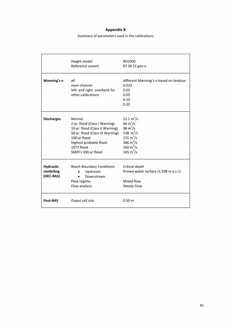
41

Appendix B

Summary of parameters used in the calibrations

Height model RH2000 Reference system RT 38 25 gon v

Manning’s n

all

different Manning’s n based on landuse

main channel 0.033 left- and right- overbank for

other calibrations 0.02 0.05 0.10 0.20

Discharges Normal 12.1 m

3/s

2-yr. flood (Class I Warning) 60 m3/s

10-yr. flood (Class II Warning) 98 m3/s

50-yr. flood (Class III Warning) 138 m3/s

100-yr flood 155 m3/s

Highest probable flood 386 m3/s

1977 flood 160 m3/s

SMHI’s 100-yr flood 165 m3/s

Hydraulic modelling (HEC-RAS)

Reach Boundary Conditions

Upstream

Downstream

Critical depth Known water surface (1.598 m a.s.l.)

Flow regime Mixed flow Flow analysis Steady Flow

Post-RAS

Ouput cell size

0.50 m

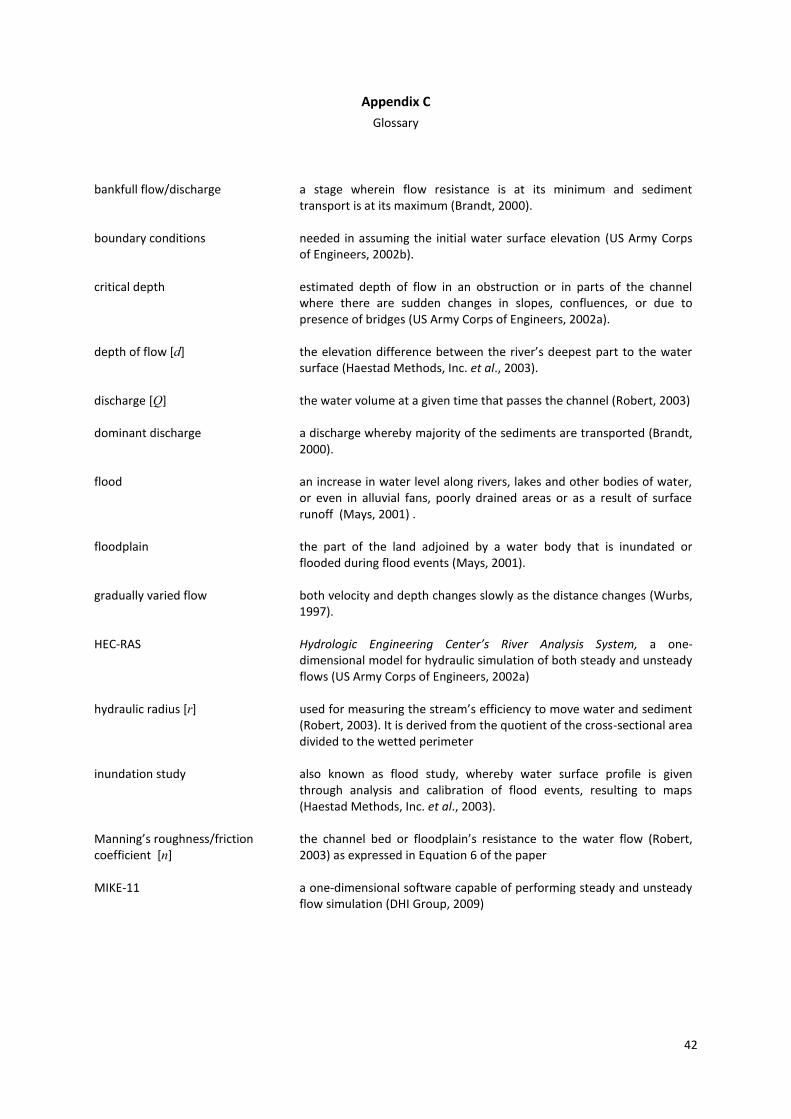
42

Appendix C

Glossary

bankfull flow/discharge a stage wherein flow resistance is at its minimum and sediment

transport is at its maximum (Brandt, 2000).

boundary conditions needed in assuming the initial water surface elevation (US Army Corps of Engineers, 2002b).

critical depth estimated depth of flow in an obstruction or in parts of the channel where there are sudden changes in slopes, confluences, or due to presence of bridges (US Army Corps of Engineers, 2002a).

depth of flow [d] the elevation difference between the river’s deepest part to the water surface (Haestad Methods, Inc. et al., 2003).

discharge [Q] the water volume at a given time that passes the channel (Robert, 2003)

dominant discharge a discharge whereby majority of the sediments are transported (Brandt, 2000).

flood an increase in water level along rivers, lakes and other bodies of water, or even in alluvial fans, poorly drained areas or as a result of surface runoff (Mays, 2001) .

floodplain the part of the land adjoined by a water body that is inundated or flooded during flood events (Mays, 2001).

gradually varied flow both velocity and depth changes slowly as the distance changes (Wurbs, 1997).

HEC-RAS Hydrologic Engineering Center’s River Analysis System, a one-dimensional model for hydraulic simulation of both steady and unsteady flows (US Army Corps of Engineers, 2002a)

hydraulic radius [r] used for measuring the stream’s efficiency to move water and sediment (Robert, 2003). It is derived from the quotient of the cross-sectional area divided to the wetted perimeter

inundation study also known as flood study, whereby water surface profile is given through analysis and calibration of flood events, resulting to maps (Haestad Methods, Inc. et al., 2003).

Manning’s roughness/friction coefficient [n]

the channel bed or floodplain’s resistance to the water flow (Robert, 2003) as expressed in Equation 6 of the paper

MIKE-11 a one-dimensional software capable of performing steady and unsteady flow simulation (DHI Group, 2009)

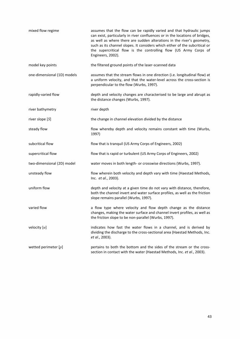
43

mixed flow regime assumes that the flow can be rapidly varied and that hydraulic jumps can exist, particularly in river confluences or in the locations of bridges, as well as where there are sudden alterations in the river’s geometry, such as its channel slopes. It considers which either of the subcritical or the supercritical flow is the controlling flow (US Army Corps of Engineers, 2002).

model key points the filtered ground points of the laser-scanned data

one-dimensional (1D) models assumes that the stream flows in one direction (i.e. longitudinal flow) at a uniform velocity, and that the water-level across the cross-section is perpendicular to the flow (Wurbs, 1997).

rapidly-varied flow depth and velocity changes are characterised to be large and abrupt as the distance changes (Wurbs, 1997).

river bathymetry river depth

river slope [S] the change in channel elevation divided by the distance

steady flow flow whereby depth and velocity remains constant with time (Wurbs, 1997)

subcritical flow flow that is tranquil (US Army Corps of Engineers, 2002)

supercritical flow flow that is rapid or turbulent (US Army Corps of Engineers, 2002)

two-dimensional (2D) model water moves in both length- or crosswise directions (Wurbs, 1997).

unsteady flow flow wherein both velocity and depth vary with time (Haestad Methods, Inc. et al., 2003).

uniform flow depth and velocity at a given time do not vary with distance, therefore, both the channel invert and water surface profiles, as well as the friction slope remains parallel (Wurbs, 1997).

varied flow a flow type where velocity and flow depth change as the distance changes, making the water surface and channel invert profiles, as well as the friction slope to be non-parallel (Wurbs, 1997).

velocity [u] indicates how fast the water flows in a channel, and is derived by dividing the discharge to the cross-sectional area (Haestad Methods, Inc. et al., 2003).

wetted perimeter [p] pertains to both the bottom and the sides of the stream or the cross-section in contact with the water (Haestad Methods, Inc. et al., 2003).

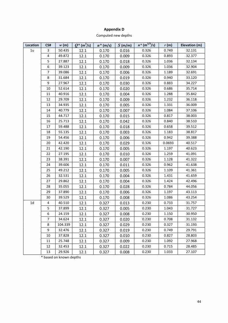
44

Appendix D

Computed new depths

Location CS# w (m) Q* (m3/s) u* (m/s) S (m/m) n* (m

1/3/s) r (m) Elevation (m)

1u 3 50.435 12.1 0.170 0.016 0.326 0.749 32.131

4 49.872 12.1 0.170 0.009 0.326 0.893 32.377

5 27.887 12.1 0.170 0.018 0.326 1.036 32.134

6 39.123 12.1 0.170 0.009 0.326 1.036 32.904

7 39.086 12.1 0.170 0.006 0.326 1.189 32.691

8 31.684 12.1 0.170 0.019 0.326 0.940 33.120

9 27.967 12.1 0.170 0.030 0.326 0.883 34.227

10 52.614 12.1 0.170 0.020 0.326 0.686 35.714

11 40.916 12.1 0.170 0.004 0.326 1.288 35.842

12 29.709 12.1 0.170 0.009 0.326 1.232 36.118

13 34.935 12.1 0.170 0.005 0.326 1.331 36.009

14 40.779 12.1 0.170 0.007 0.326 1.084 37.106

15 44.717 12.1 0.170 0.015 0.326 0.817 38.003

16 25.713 12.1 0.170 0.042 0.326 0.840 38.510

17 59.488 12.1 0.170 0.018 0.326 0.658 39.512

18 55.135 12.1 0.170 0.003 0.326 1.183 38.817

19 54.456 12.1 0.170 0.006 0.326 0.942 39.388

20 42.420 12.1 0.170 0.029 0.326 0.0693 40.517

21 42.190 12.1 0.170 0.005 0.326 1.197 40.623

22 27.195 12.1 0.170 0.010 0.326 1.259 41.091

23 38.391 12.1 0.170 0.007 0.326 1.128 41.322

24 39.606 12.1 0.170 0.011 0.326 0.962 41.638

25 49.212 12.1 0.170 0.005 0.326 1.109 41.361

26 32.531 12.1 0.170 0.004 0.326 1.431 41.659

27 29.862 12.1 0.170 0.004 0.326 1.424 42.496

28 35.055 12.1 0.170 0.028 0.326 0.784 44.056

29 37.890 12.1 0.170 0.006 0.326 1.197 43.113

30 39.529 12.1 0.170 0.008 0.326 1.086 43.254

1d 4 40.510 12.1 0.327 0.013 0.230 0.733 31.757

5 37.899 12.1 0.327 0.005 0.230 1.043 31.727

6 24.159 12.1 0.327 0.008 0.230 1.150 30.950

7 34.624 12.1 0.327 0.020 0.230 0.708 31.132

8 104.339 12.1 0.327 0.029 0.230 0.327 31.193

9 32.476 12.1 0.327 0.019 0.230 0.749 29.791

10 37.828 12.1 0.327 0.010 0.230 0.827 28.803

11 25.748 12.1 0.327 0.009 0.230 1.092 27.968

12 32.453 12.1 0.327 0.022 0.230 0.715 28.485

13 29.926 12.1 0.327 0.008 0.230 1.033 27.107

* based on known depths

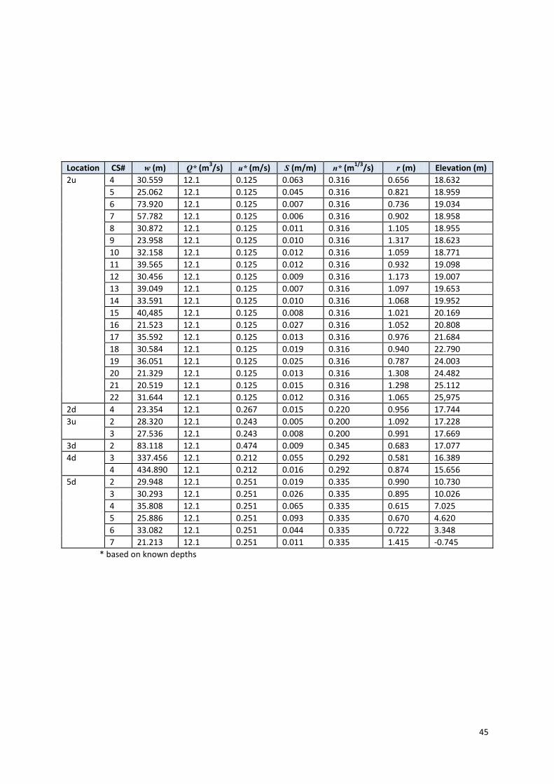
45

Location CS# w (m) Q* (m3/s) u* (m/s) S (m/m) n* (m

1/3/s) r (m) Elevation (m)

2u 4 30.559 12.1 0.125 0.063 0.316 0.656 18.632

5 25.062 12.1 0.125 0.045 0.316 0.821 18.959

6 73.920 12.1 0.125 0.007 0.316 0.736 19.034

7 57.782 12.1 0.125 0.006 0.316 0.902 18.958

8 30.872 12.1 0.125 0.011 0.316 1.105 18.955

9 23.958 12.1 0.125 0.010 0.316 1.317 18.623

10 32.158 12.1 0.125 0.012 0.316 1.059 18.771

11 39.565 12.1 0.125 0.012 0.316 0.932 19.098

12 30.456 12.1 0.125 0.009 0.316 1.173 19.007

13 39.049 12.1 0.125 0.007 0.316 1.097 19.653

14 33.591 12.1 0.125 0.010 0.316 1.068 19.952

15 40,485 12.1 0.125 0.008 0.316 1.021 20.169

16 21.523 12.1 0.125 0.027 0.316 1.052 20.808

17 35.592 12.1 0.125 0.013 0.316 0.976 21.684

18 30.584 12.1 0.125 0.019 0.316 0.940 22.790

19 36.051 12.1 0.125 0.025 0.316 0.787 24.003

20 21.329 12.1 0.125 0.013 0.316 1.308 24.482

21 20.519 12.1 0.125 0.015 0.316 1.298 25.112

22 31.644 12.1 0.125 0.012 0.316 1.065 25,975

2d 4 23.354 12.1 0.267 0.015 0.220 0.956 17.744

3u 2 28.320 12.1 0.243 0.005 0.200 1.092 17.228

3 27.536 12.1 0.243 0.008 0.200 0.991 17.669

3d 2 83.118 12.1 0.474 0.009 0.345 0.683 17.077

4d 3 337.456 12.1 0.212 0.055 0.292 0.581 16.389

4 434.890 12.1 0.212 0.016 0.292 0.874 15.656

5d 2 29.948 12.1 0.251 0.019 0.335 0.990 10.730

3 30.293 12.1 0.251 0.026 0.335 0.895 10.026

4 35.808 12.1 0.251 0.065 0.335 0.615 7.025

5 25.886 12.1 0.251 0.093 0.335 0.670 4.620

6 33.082 12.1 0.251 0.044 0.335 0.722 3.348

7 21.213 12.1 0.251 0.011 0.335 1.415 -0.745

* based on known depths

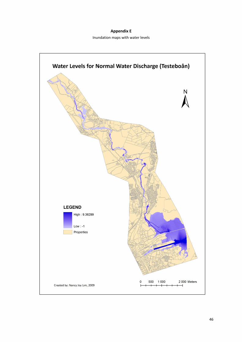
46

Appendix E

Inundation maps with water levels

47

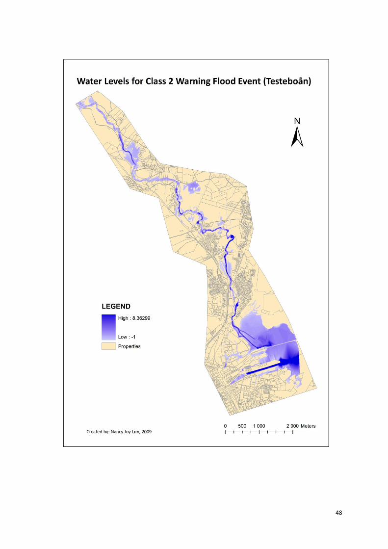
48

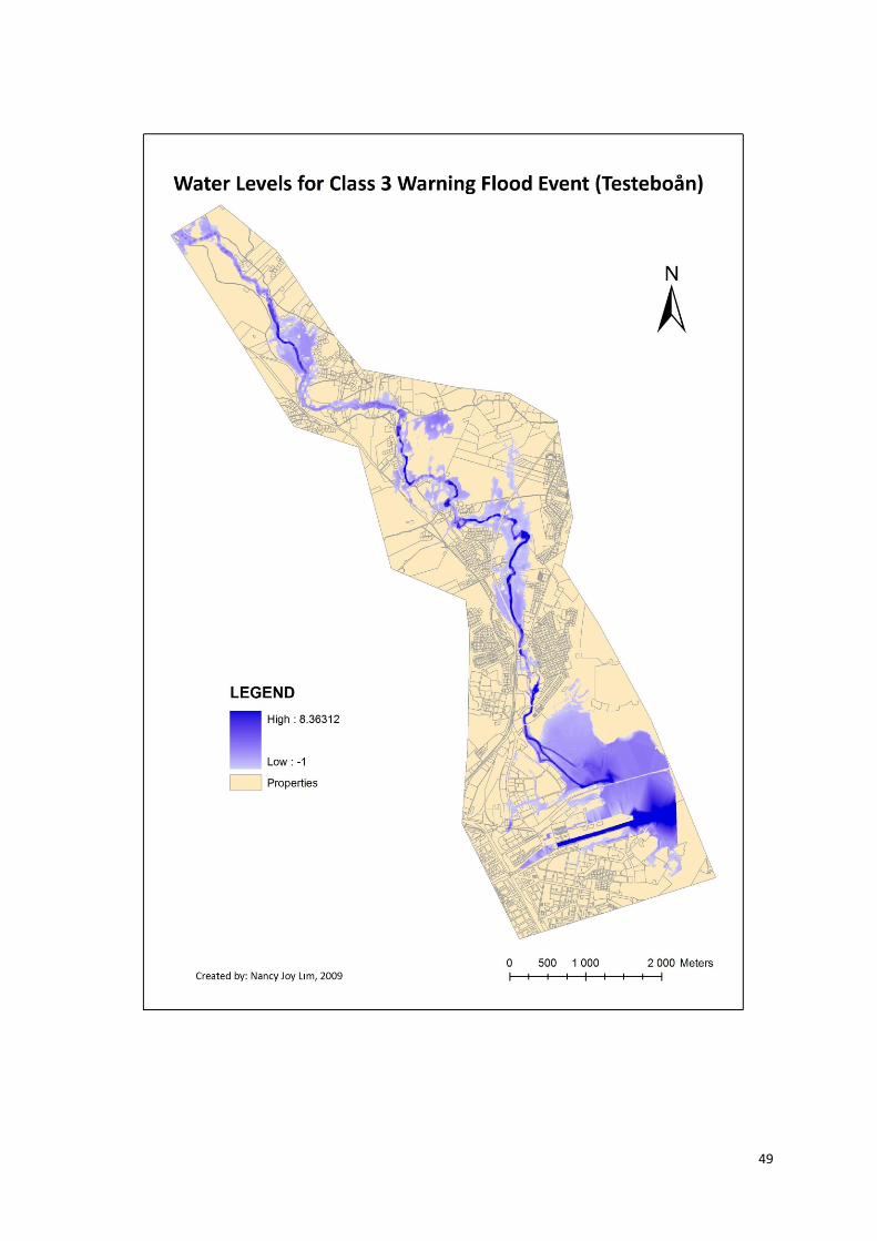
49

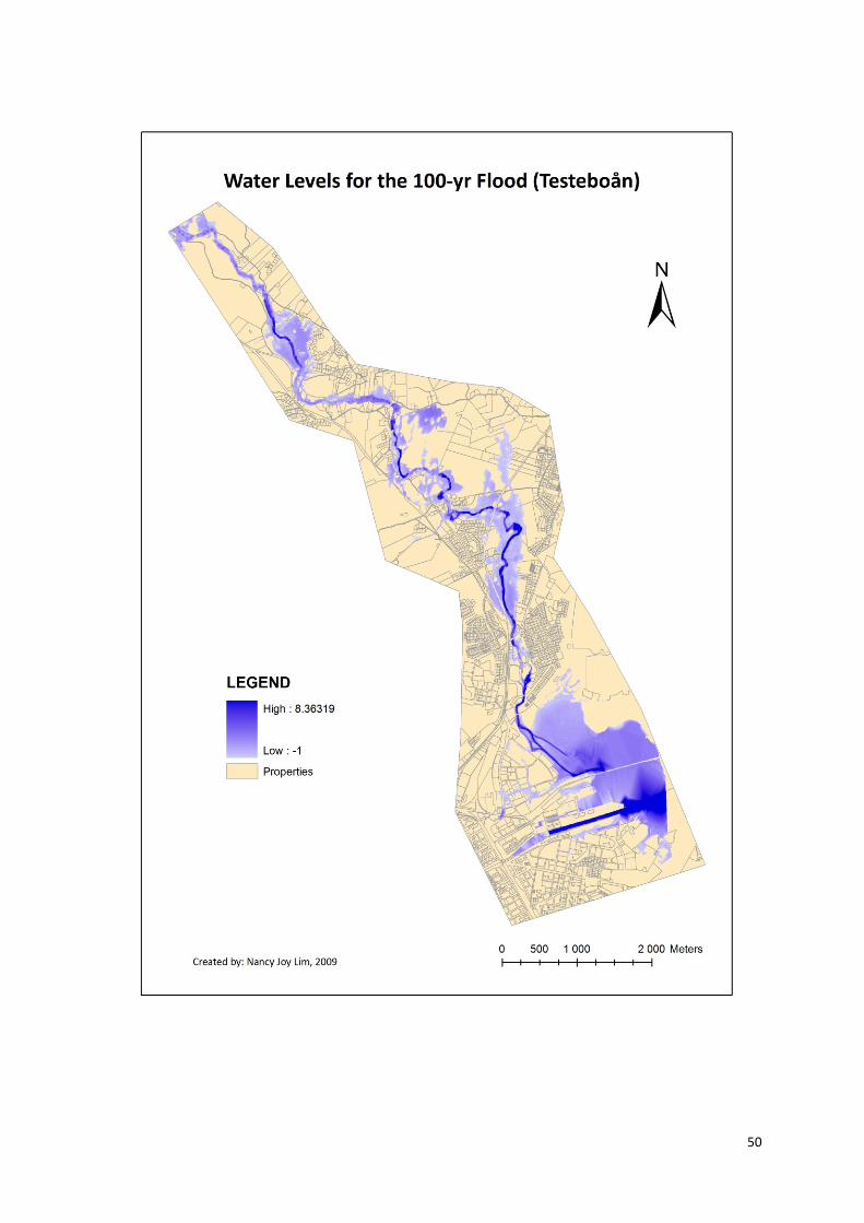
50

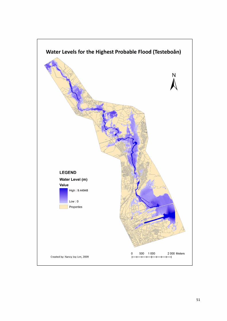
51

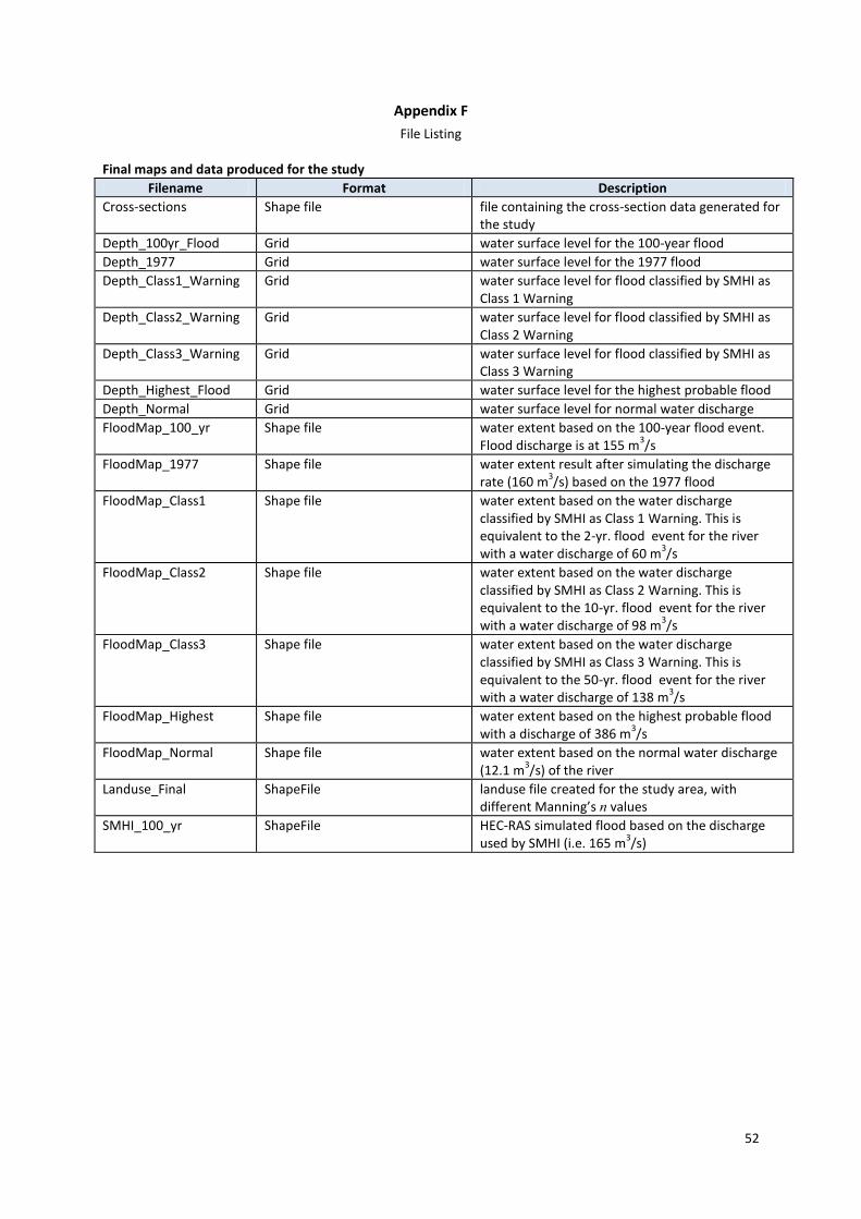
52

Appendix F

File Listing Final maps and data produced for the study

Filename Format Description

Cross-sections Shape file file containing the cross-section data generated for the study

Depth_100yr_Flood Grid water surface level for the 100-year flood

Depth_1977 Grid water surface level for the 1977 flood

Depth_Class1_Warning Grid water surface level for flood classified by SMHI as Class 1 Warning

Depth_Class2_Warning Grid water surface level for flood classified by SMHI as Class 2 Warning

Depth_Class3_Warning Grid water surface level for flood classified by SMHI as Class 3 Warning

Depth_Highest_Flood Grid water surface level for the highest probable flood

Depth_Normal Grid water surface level for normal water discharge

FloodMap_100_yr Shape file water extent based on the 100-year flood event. Flood discharge is at 155 m

3/s

FloodMap_1977 Shape file water extent result after simulating the discharge rate (160 m

3/s) based on the 1977 flood

FloodMap_Class1 Shape file water extent based on the water discharge classified by SMHI as Class 1 Warning. This is equivalent to the 2-yr. flood event for the river with a water discharge of 60 m

3/s

FloodMap_Class2 Shape file water extent based on the water discharge classified by SMHI as Class 2 Warning. This is equivalent to the 10-yr. flood event for the river with a water discharge of 98 m

3/s

FloodMap_Class3 Shape file water extent based on the water discharge classified by SMHI as Class 3 Warning. This is equivalent to the 50-yr. flood event for the river with a water discharge of 138 m

3/s

FloodMap_Highest Shape file water extent based on the highest probable flood with a discharge of 386 m

3/s

FloodMap_Normal Shape file water extent based on the normal water discharge (12.1 m

3/s) of the river

Landuse_Final ShapeFile landuse file created for the study area, with different Manning’s n values

SMHI_100_yr ShapeFile HEC-RAS simulated flood based on the discharge used by SMHI (i.e. 165 m

3/s)

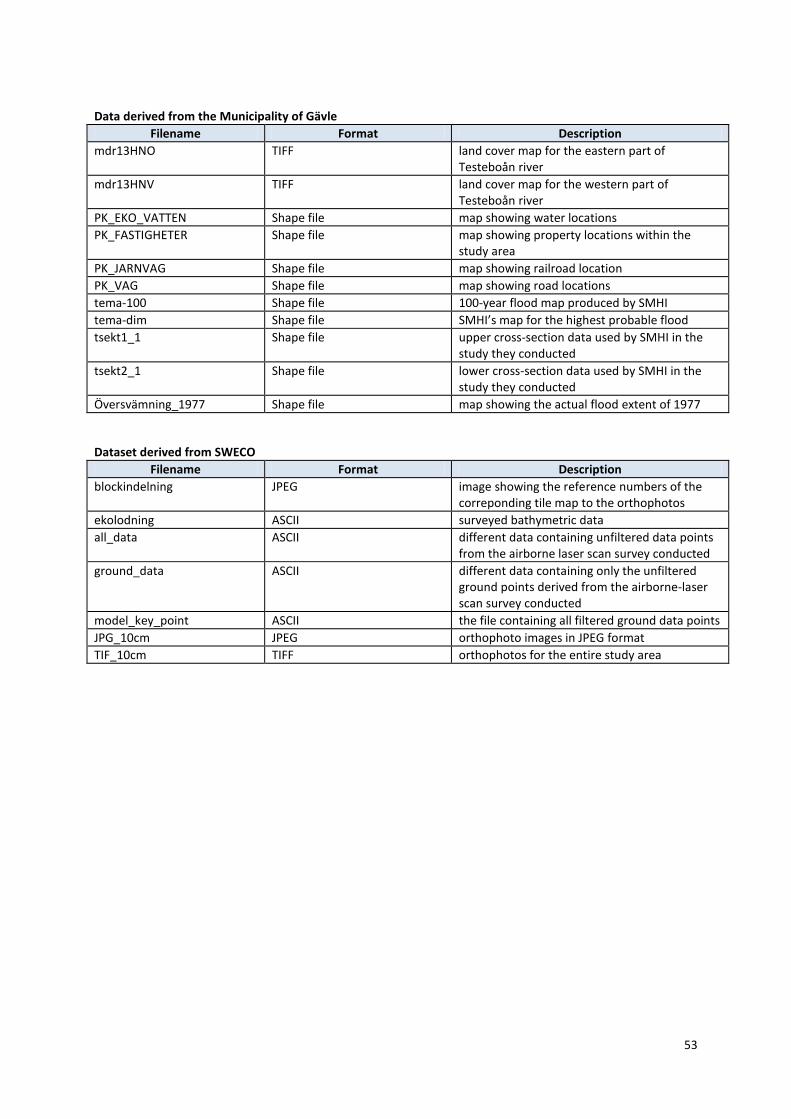
53

Data derived from the Municipality of Gävle

Filename Format Description

mdr13HNO TIFF land cover map for the eastern part of Testeboån river

mdr13HNV TIFF land cover map for the western part of Testeboån river

PK_EKO_VATTEN Shape file map showing water locations

PK_FASTIGHETER Shape file map showing property locations within the study area

PK_JARNVAG Shape file map showing railroad location

PK_VAG Shape file map showing road locations

tema-100 Shape file 100-year flood map produced by SMHI

tema-dim Shape file SMHI’s map for the highest probable flood

tsekt1_1 Shape file upper cross-section data used by SMHI in the study they conducted

tsekt2_1 Shape file lower cross-section data used by SMHI in the study they conducted

Översvämning_1977 Shape file map showing the actual flood extent of 1977

Dataset derived from SWECO

Filename Format Description

blockindelning JPEG image showing the reference numbers of the correponding tile map to the orthophotos

ekolodning ASCII surveyed bathymetric data

all_data ASCII different data containing unfiltered data points from the airborne laser scan survey conducted

ground_data ASCII different data containing only the unfiltered ground points derived from the airborne-laser scan survey conducted

model_key_point ASCII the file containing all filtered ground data points

JPG_10cm JPEG orthophoto images in JPEG format

TIF_10cm TIFF orthophotos for the entire study area

54