TOPOCLIMATIC MODELING OF THERMOPLUVIOMETRIC VARIABLES FOR THE BÍO BÍO AND LA ARAUCANÍA REGIONS, CHILE

604 CHIL. J. AGR. RES. - VOL. 70 - Nº 4 - 2010RESEARCH

CHILEAN JOURNAL OF AGRICULTURAL RESEARCH 70(4):604-615 (OCTOBER-DECEMBER 2010)

TOPOCLIMATIC MODELING OF THERMOPLUVIOMETRIC VARIABLES FOR THE BÍO BÍO AND LA ARAUCANÍA REGIONS, CHILE

Diego Díaz M.1*, Luis Morales S.2, Giorgio Castellaro G.2, and Fernando Neira R2.

ABSTRACT

Climatic mapping in the Bío Bío and La Araucanía Regions of Chile is primarily in analog form (paper) and delineation of contours, making it unsuitable for digital handling by geographic information systems (GIS). Therefore, in this study, topoclimatic models were created and spatially represented to explain the spatial and temporal variation of monthly mean temperature and precipitation, as a function of variability and singularity of the physiographic characteristics of the Bío Bío and La Araucanía Regions. The physiographic factors considered were latitude, longitude, altitude, aspect and distance to coastline. To elaborate equations, data from thermopluviometric stations of the study area were compiled and systematized. These stations were standardized to a common reference system in order to locate them in space and obtain the value of physiographic factors for each station. With this information, the equations were calculated using a stepwise (backward) regression procedure, with a statistical significance of 95%. The regression equations obtained for mean monthly and annual temperature and precipitation were all significant (P ≤ 0.05) and had R2 > 0.7. These equations were applied to the rest of the study area in raster format using a GIS, which yields a spatially continuous cartography. The spatial resolution or pixel size was 90 m, which allows carrying out research at a 1:100 000 scale, commonly used at the regional or provincial level.

Key words: Topoclimatic models, mean temperature, mean precipitation, pluviometric cartographic, GIS.

1Centro Nacional del Medio Ambiente – CENMA, Laboratorio de Modelación e Inventario de Emisiones, Casilla 7880096, Santiago, Chile. *Corresponding author ([email protected]).2Universidad de Chile, Facultad de Ciencias Agronómicas, Casilla 1004, Santiago, Chile.Received: 25 August 2009.Accepted: 8 December 2009.

INTRODUCTION

Climate, defined as the mean state of the atmosphere in a determined place, is a variable that affects, models and conditions biological, physical and chemical processes that occur in nature (Hufty, 1984). The elements influenced by climate are geography, soil characteristics, vegetation, and ultimately the use and occupation of a determined territory. Because of this, the climatic variable is a conditioning factor in the planning of human activities (Romero and Martínez, 2001). If we consider the importance of climate for the processes that occur in nature and the possible variations of climate owing to physiographic factors, it is necessary to have base climatic information to undertake any study about a determined territory.

This is relevant for Chile, where the physiographic factors are highly variable, with a latitudinal range of approximately 38º (Di Castri and Hajek, 1976), altitudes that range from 0 to 6000 m.a.s.l. and a marked maritime influence (Errázuriz et al., 1994). The study of climatic variation attributable to physiographic factors has been undertaken using what is termed “topoclimatic analysis”, which is defined in general terms as the climatic characteristics of a place that can be described as a combination of topographic parameters (Okolowicz, 1969, cited by Kaminski and Radosz, 2005). The cartographic representation of climatic variables has generally been carried out manually, subject to expert criteria, such as isothermal and isohyet maps, which are isolines that join points with the same temperature and the same level of precipitation, respectively. These isolines are drawn on the basis of an altitudinal gradient, considering the values registered each year from observatories in the zone, the density of which conditions the interval of its plotting (Fernández, 1996). As an alternative to this method of representation, different interpolation algorithms have been developed and automated to estimate and predict the spatial distribution of a variable based on timely data generated by meteorological stations (Hijmans et

605D. DÍAZ et al. - TOPOCLIMATIC MODELING OF THERMOPLUVIOMETRIC…

al., 2005; Hunter and Meentemeyer, 2005; Attorre et al., 2007). The processes of obtaining climatic cartography, whether through the use of a traditional methods (analogic) or an automated method, is conditioned by the availability and quality of climatic information or data that comes mainly from meteorological stations located in particular points in space (Skirvin et al., 2003; Morales et al., 2006) that often do not cover the totality of a region, leaving areas without information. Given this, models are developed that allow for spatially representing the monthly distribution of temperature and precipitation on an ongoing basis, using Geographic Information System (GIS) raster, obtaining Digital Terrain Models (DTM), which are spatial representations of continuous variables (Doyle, 1978; cited by Florinsky, 1998; Daly et al., 2008). Given the importance of having climatic information to develop studies in a determined area, and considering the physiographic variability of Chile associated with the lack of good coverage by meteorological stations and the continuous character of the distribution of climatic variables, this study aims to generate estimation models of climatic information that allow for continuously characterizing the whole territory, taking into consideration physiographic variables.

MATERIALS AND METHODS

Area of studyThe study was carried out in the Bío Bío and La Araucanía Regions, central Chile (36°0’ to 39°38’ S; 70°49’ to 73°57’ W) covering an approximate surface area of 68 704 km² (Figure 1). The Bío Bío Region marks a transition from the temperate climate that characterizes the central zone of Chile and the rainier climate characteristic of areas south of the Laja River. The characteristics of a temperate Mediterranean climate predominate in this

region. Nevertheless, differences are observed within the territory, fundamentally owing to the effect of the latitudinal gradient and the distance from the coast. The La Araucanía Region presents two well-differentiated climatic typologies, the first located in the intermediate zone in the north of the region until around 39º S lat, characterized by precipitation distributed throughout the year and a relatively short dry season of no more than 3 or 4 months during the summer. The second zone is characterized by a temperate rainy climate with Mediterranean influence, while extends until Castro in the Los Lagos Region.

Climatic and topographic data Data was used for this research from stations with ten or more years history of taking climatic measurements (Table 1) derived from: Climatology in Chile (United Nations Development Program [UNDP] - Government of Chile, 1964), Agroclimatic Map of Chile (INIA, 1989), General Water Directorate (DGA) and yearbooks from the Meteorological Directorate of Chile (DMC). To spatially represent the equations, four Digital Terrain Models were used, with information on latitude, longitude, exposure and distance from the coast, and a Digital Elevation Model obtained from the Shuttle Radar Topography Mission (SRTM), of the United States Geological Survey (USGS, 2004), all of them with a pixel size of 90 m. To adjust the temperature model, only the stations that had data for more than 10 yr were considered, from the four aforementioned sources. On the other hand, owing to the greater spatial and temporal variability of precipitation, only data from DGA stations with ten or more years of sampling records were used (Table 2). For the development, adjustment and spatial representation of topoclimatic models, it is necessary to homogenize the information, given that the stations that provide

Figure 1. The areas of the study, the Bío Bío and La Araucanía Regions.

606 CHIL. J. AGR. RES. - VOL. 70 - Nº 4 - 2010

information have different reference systems, so that all the information of a geographic character was worked in the World Geodetic System (WGS84) in spherical coordinates. Subsequently, the database was completed that was used for the generation and spatial representation of the topoclimatic models. The physiographic variables included in this study were altitude, latitude, longitude and distance from the coast. All these variables were represented with a pixel resolution of 90 m, which was used for the spatial representation of topoclimatic models and is responsible for the continuous character of the cartographies of temperature and precipitation that were generated. Once the equations have been estimated, thematic cartographies of a continuous character were developed using the computer program IDRISI® (IDRISI

32, Clark Labs, Clark University, Massachusetts, USA) and the MDTs of latitude, longitude, altitude and distance to the coast.

Topoclimatic modelingThe modeling of different climatic variables was done by applying a mathematical model described by Equation [1]: F(x1,x2,....xn)= [1]

where F(x1, x2 ,.....xn) represents a climatological variable in a given period of time, x is a descriptor variable, which can be latitude, longitude, altitude, distance from the coast or slope, among others, and aj are coefficients to be determined (Qiyao et al., 1991; Canessa, 2006). With

aj x x ....x n1 k1

n2 k2

nm km∑

j,kn,m=0

Cauquenes -35.971 -72.336 142 28.05 22 NEChillán Viejo -36.633 -72.126 140 70.78 15 NEB. O’Higgins Chillán -36.571 -72.036 124 76.50 16 1982/1997Punta Tumbes -36.624 -73.102 120 0.61 30 1916/1945Caracol -36.651 -71.389 725 133.90 20 1988/2007Embalse Coihueco -36.638 -71.797 330 98.94 31 1977/2007Talcahuano -36.721 -73.119 84 0.97 18 NECarriel Sur Concepción -36.771 -73.052 12 3.94 16 1982/1997Concepción -36.837 -73.036 10 10.58 20 NEDiguillín -36.868 -71.643 710 120.31 38 1970/2007Quilaco -37.686 -72.006 225 119.58 38 1970/2007Angol -37.804 -72.702 79 71.64 15 NEContulmo -38.012 -73.228 60 20.91 19 1988/2007Laguna Malleco -38.213 -71.814 959 143.76 18 1990/2007Traiguén -38.256 -72.654 189 70.90 26 1979/2004Lonquimay -38.455 -71.365 878 180.19 16 1992/2007Malalcahuello -38.471 -71.571 900 162.58 16 1989/2004Lautaro -38.534 -72.434 240 89.59 10 1995/2004Liucura -38.646 -71.091 1035 196.44 20 1988/2007Carillanca -38.687 -72.419 200 84.95 25 NETemuco -38.771 -72.636 114 64.07 26 1920/1945Maquehue Temuco -38.754 -72.636 114 64.78 16 1982/1997Puerto Saavedra -38.793 -73.396 5 1.26 25 1979/2004Tricauco -38.844 -71.554 518 151.67 16 1989/2004Teodoro Schmidt -39.003 -73.095 47 18.17 16 1989/2004Pucón -39.289 -71.927 200 110.62 19 1986/2004Loncoche -39.371 -72.636 31 49.02 14 NEPuesto (Aduana) -39.534 -71.557 726 143.11 17 1988/2004Pichoy Valdivia -39.621 -73.086 19 17.10 15 1982/1984-1986/1997

Table 1. Meteorological stations used in the temperature models.

NE: not specific (INIA, 1989).

LatitudeStation Longitude Altitude Years PeriodDistance to coast

degrees m.a.s.l. km

607

Embalse Tutuven -35.901 -72.376 400 20.662 28 1977/2004Embalse Ancoa -35.922 -71.287 430 116.472 30 1975/2004Los Huinganes -35.941 -71.942 132 58.817 11 1994/2004Liguay -35.948 -71.690 145 81.068 30 1975/2004Quella -36.061 -72.092 130 51.920 30 1975/2004Mangarral -36.233 -72.342 150 42.189 13 1992/2004Millauquen -36.316 -72.038 130 69.509 13 1992/2004San Agustín de Puñual -36.352 -72.393 100 38.349 12 1993/2004Coelemu -36.484 -72.698 30 16.995 30 1975/2004Dichato -36.546 -72.931 4 0.298 25 1980/2004San Fabián -36.561 -71.548 500 117.421 30 1975/2004Chillán Viejo -36.633 -72.126 140 70.776 28 1977/2004Rafael -36.637 -72.844 198 10.099 12 1993/2004Embalse Coihueco -36.638 -71.797 330 98.937 30 1975/2004Caracol -36.651 -71.389 725 133.896 18 1987/2004Nueva Aldea -36.653 -72.455 60 43.985 30 1975/2004Caman -36.674 -71.298 920 142.368 12 1993/2004Cancha Los Litres -36.705 -72.578 250 34.888 12 1993/2004Chillancito -36.761 -72.421 70 49.872 30 1975/2004Las Pataguas -36.790 -72.891 250 11.022 12 1993/2004Mayulermo -36.817 -71.893 375 97.221 13 1992/2004Diguillín -36.868 -71.643 710 120.308 30 1975/2004Las Trancas -36.910 -71.477 1160 135.700 30 1975/2004Fundo Atacalco -36.916 -71.579 730 126.850 30 1975/2004Pemuco -36.977 -72.096 200 83.993 30 1975/2004Las Cruces -37.109 -71.766 650 116.663 12 1993/2004Cholguán -37.152 -72.066 225 94.780 30 1975/2004Laja -37.271 -72.719 40 42.258 30 1975/2004Trupán -37.279 -71.822 460 119.539 30 1975/2004Tucapel -37.294 -71.952 330 108.433 30 1975/2004Fundo Las Achiras -37.354 -72.386 125 73.155 30 1975/2004Los Ángeles -37.502 -72.407 120 78.696 30 1975/2004Fundo San Lorenzo -37.509 -71.768 740 130.430 30 1975/2004San Carlos de Purén -37.595 -72.277 150 93.836 20 1985/2004Quillaileo -37.653 -71.712 500 141.067 12 1993/2004Quilaco -37.686 -72.006 225 119.578 30 1975/2004Mulchen -37.716 -72.244 130 103.532 30 1975/2004Angol (La Mona) -37.779 -72.637 154 78.003 25 1975/1990-1996/2004Cerro El Padre -37.780 -71.865 400 135.501 30 1975/2004Cañete -37.798 -73.391 25 15.608 30 1975/2004Pilguen -37.832 -72.219 300 111.884 12 1993/2004Poco a Poco -37.872 -71.993 650 130.592 13 1992/2004Collipulli -37.955 -72.442 257 90.200 30 1975/2004Contulmo -38.012 -73.228 60 20.915 17 1987/1989-1991/2004Tranaman -38.021 -73.009 55 39.732 17 1988/2004

Table 2. Meteorological stations used in the temperature models.


degrees m.a.s.l. km

D. DÍAZ et al. - TOPOCLIMATIC MODELING OF THERMOPLUVIOMETRIC…


Encimar Malleco -38.104 -72.117 420 117.025 16 1989/2004Lumaco -38.164 -72.902 127 48.305 30 1975/2004Laguna Malleco -38.213 -71.814 959 143.761 30 1975/2004Las Mercedes, Victoria -38.243 -72.210 466 109.370 19 1986/2004Traiguén -38.256 -72.654 189 70.904 26 1979/2004Galvarino -38.410 -72.786 58 62.716 26 1979/2004Rari-Ruca -38.425 -72.011 361 128.381 13 1992/2004Curacautín -38.437 -71.885 499 138.398 30 1975/2004Quillén -38.464 -72.386 275 95.918 30 1975/2004Malalcahuello -38.471 -71.571 900 162.582 16 1989/2004La Cabaña -38.530 -73.121 709 33.204 16 1989/2004Lautaro -38.534 -72.434 240 89.591 30 1975/2004Chochol -38.609 -72.845 72 52.739 17 1988/2004Vilcún -38.672 -72.218 376 101.976 30 1975/2004Cherquenco -38.683 -72.002 528 119.496 17 1988/2004Carahue -38.713 -73.148 50 24.200 10 1995/2004Pueblo Nuevo, Temuco -38.723 -72.570 115 71.350 30 1975/2004Almagro -38.781 -72.952 20 38.231 10 1995/2004Puerto Saavedra -38.793 -73.396 5 1.263 26 1979/2004Tricauco -38.844 -71.554 518 151.667 16 1989/2004Cunco -38.929 -72.016 470 110.422 30 1975/2004Sendos Freire -38.950 -72.667 123 43.491 24 1981/2004Los Laureles -38.959 -72.188 250 95.151 30 1975/2004Quecherehua -38.998 -72.044 420 105.993 30 1975/2004Teodoro Schmidt -39.003 -73.095 47 18.172 16 1989/2004Quitratue -39.155 -72.658 88 50.106 30 1975/2004Toltén -39.181 -73.166 17 7.169 10 1995/2004Lago Caburga -39.221 -71.585 480 140.684 24 1977/2000Villarrica -39.278 -72.228 187 84.799 30 1975/2004Pucón -39.289 -71.927 200 110.619 21 1984/2004Curarrehue -39.363 -71.581 580 140.096 28 1977/2004Loncoche -39.371 -72.636 31 49.024 11 1994/2004Chanlelful -39.465 -72.375 166 72.279 17 1988/2004Puesto (Aduana) -39.534 -71.557 726 143.112 17 1988/2004Lago Calafquén -39.552 -72.152 375 92.485 18 1987/2004Liquiñe -39.731 -71.853 230 121.527 11 1994/2004Lago Riñihue -39.774 -72.453 120 73.540 20 1985/2004

Continuation Table 2.


degrees m.a.s.l. km

these relationships, the data matrices are calculated for each climatological variable in binary format (raster) for the months of January and July. The binary metrical format was used because it corresponds to the format of the IDRISI Program®, which is used for the spatial characterization of continuous variables. The proposed

topoclimatic model (Equation [1]) to estimate mean monthly temperature and precipitation considered that spatial variation of the aforementioned variables is determined by factors of position on the surface of the earth, this being latitude (LAT, degrees) and longitude (LON, degrees), as well as physiographic factors like

609

altitude (ALT, m.a.s.l.) and distance to the coast (DL, km), as shown in Equation [2].

Y = a0 + alLAT + a2LON + a3ALT + a4DL [2]

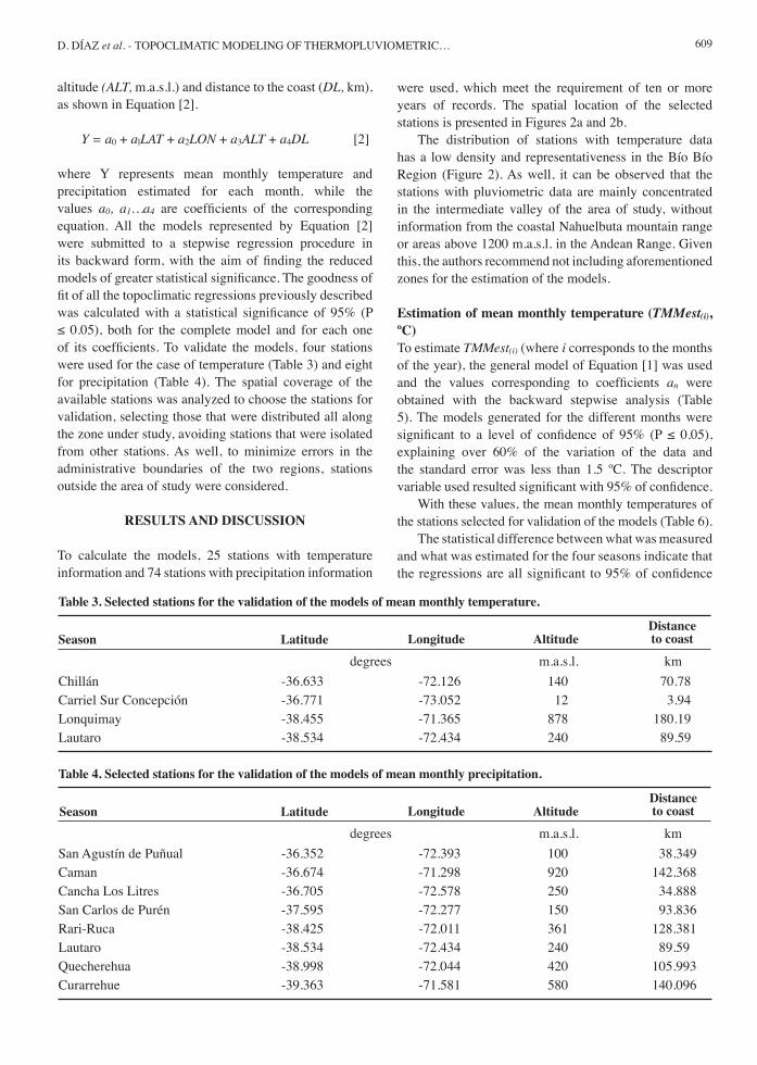
where Y represents mean monthly temperature and precipitation estimated for each month, while the values a0, a1…a4 are coefficients of the corresponding equation. All the models represented by Equation [2] were submitted to a stepwise regression procedure in its backward form, with the aim of finding the reduced models of greater statistical significance. The goodness of fit of all the topoclimatic regressions previously described was calculated with a statistical significance of 95% (P ≤ 0.05), both for the complete model and for each one of its coefficients. To validate the models, four stations were used for the case of temperature (Table 3) and eight for precipitation (Table 4). The spatial coverage of the available stations was analyzed to choose the stations for validation, selecting those that were distributed all along the zone under study, avoiding stations that were isolated from other stations. As well, to minimize errors in the administrative boundaries of the two regions, stations outside the area of study were considered.

RESULTS AND DISCUSSION

To calculate the models, 25 stations with temperature information and 74 stations with precipitation information


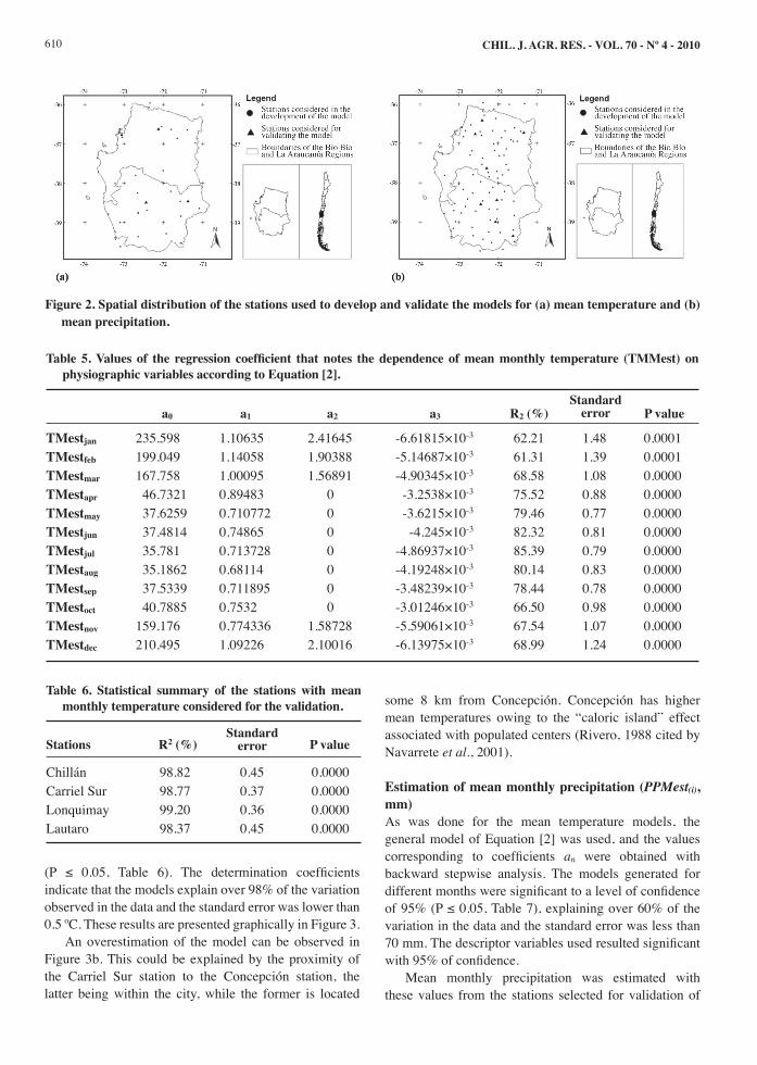
were used, which meet the requirement of ten or more years of records. The spatial location of the selected stations is presented in Figures 2a and 2b. The distribution of stations with temperature data has a low density and representativeness in the Bío Bío Region (Figure 2). As well, it can be observed that the stations with pluviometric data are mainly concentrated in the intermediate valley of the area of study, without information from the coastal Nahuelbuta mountain range or areas above 1200 m.a.s.l. in the Andean Range. Given this, the authors recommend not including aforementioned zones for the estimation of the models.

Estimation of mean monthly temperature (TMMest(i), ºC)To estimate TMMest(i) (where i corresponds to the months of the year), the general model of Equation [1] was used and the values corresponding to coefficients an were obtained with the backward stepwise analysis (Table 5). The models generated for the different months were significant to a level of confidence of 95% (P ≤ 0.05), explaining over 60% of the variation of the data and the standard error was less than 1.5 ºC. The descriptor variable used resulted significant with 95% of confidence. With these values, the mean monthly temperatures of the stations selected for validation of the models (Table 6). The statistical difference between what was measured and what was estimated for the four seasons indicate that the regressions are all significant to 95% of confidence

Chillán -36.633 -72.126 140 70.78Carriel Sur Concepción -36.771 -73.052 12 3.94Lonquimay -38.455 -71.365 878 180.19Lautaro -38.534 -72.434 240 89.59

Table 3. Selected stations for the validation of the models of mean monthly temperature.

LatitudeSeason Longitude AltitudeDistance to coast

degrees m.a.s.l. km

San Agustín de Puñual -36.352 -72.393 100 38.349Caman -36.674 -71.298 920 142.368Cancha Los Litres -36.705 -72.578 250 34.888San Carlos de Purén -37.595 -72.277 150 93.836Rari-Ruca -38.425 -72.011 361 128.381Lautaro -38.534 -72.434 240 89.59Quecherehua -38.998 -72.044 420 105.993Curarrehue -39.363 -71.581 580 140.096

Table 4. Selected stations for the validation of the models of mean monthly precipitation.

LatitudeSeason Longitude AltitudeDistance to coast

degrees m.a.s.l. km


(P ≤ 0.05, Table 6). The determination coefficients indicate that the models explain over 98% of the variation observed in the data and the standard error was lower than 0.5 ºC. These results are presented graphically in Figure 3. An overestimation of the model can be observed in Figure 3b. This could be explained by the proximity of the Carriel Sur station to the Concepción station, the latter being within the city, while the former is located

some 8 km from Concepción. Concepción has higher mean temperatures owing to the “caloric island” effect associated with populated centers (Rivero, 1988 cited by Navarrete et al., 2001).

Estimation of mean monthly precipitation (PPMest(i), mm)As was done for the mean temperature models, the general model of Equation [2] was used, and the values corresponding to coefficients an were obtained with backward stepwise analysis. The models generated for different months were significant to a level of confidence of 95% (P ≤ 0.05, Table 7), explaining over 60% of the variation in the data and the standard error was less than 70 mm. The descriptor variables used resulted significant with 95% of confidence. Mean monthly precipitation was estimated with these values from the stations selected for validation of

TMestjan 235.598 1.10635 2.41645 -6.61815×10-3 62.21 1.48 0.0001TMestfeb 199.049 1.14058 1.90388 -5.14687×10-3 61.31 1.39 0.0001TMestmar 167.758 1.00095 1.56891 -4.90345×10-3 68.58 1.08 0.0000TMestapr 46.7321 0.89483 0 -3.2538×10-3 75.52 0.88 0.0000TMestmay 37.6259 0.710772 0 -3.6215×10-3 79.46 0.77 0.0000TMestjun 37.4814 0.74865 0 -4.245×10-3 82.32 0.81 0.0000TMestjul 35.781 0.713728 0 -4.86937×10-3 85.39 0.79 0.0000TMestaug 35.1862 0.68114 0 -4.19248×10-3 80.14 0.83 0.0000TMestsep 37.5339 0.711895 0 -3.48239×10-3 78.44 0.78 0.0000TMestoct 40.7885 0.7532 0 -3.01246×10-3 66.50 0.98 0.0000TMestnov 159.176 0.774336 1.58728 -5.59061×10-3 67.54 1.07 0.0000TMestdec 210.495 1.09226 2.10016 -6.13975×10-3 68.99 1.24 0.0000

Table 5. Values of the regression coefficient that notes the dependence of mean monthly temperature (TMMest) on physiographic variables according to Equation [2].

a0 a1 a2 a3 R2 (%) P valueStandard

error

Chillán 98.82 0.45 0.0000Carriel Sur 98.77 0.37 0.0000Lonquimay 99.20 0.36 0.0000Lautaro 98.37 0.45 0.0000

Table 6. Statistical summary of the stations with mean monthly temperature considered for the validation.

StationsStandard

errorR2 (%) P value

Figure 2. Spatial distribution of the stations used to develop and validate the models for (a) mean temperature and (b) mean precipitation.

611

the models. The regression statistics for the validation stations are presented in Table 8. The statistical difference between what was measured and what was estimated for the eight stations of validation indicate that the regressions are all significant to 95% of confidence (P ≤ 0.05). The determination coefficients indicate that the models explain over 92% of the variation observed in the data and the standard error was less than 32 mm (Table 8). The graphic representation of the models for the eight seasons is presented in Figure 4.

The calculated models show significant statistical values (P ≤ 0.05), and the values of R2 in the majority of the estimations are higher than 70%. These values are within the range of those obtained in other studies of a topoclimatic character undertaken in Europe by Ninyerola et al. (2000), who reports values of R2 higher than 70% for the estimation of precipitation and higher than 86% temperature. In turn, the studies of Goodale et al. (1998) indicate values higher than 69% for the estimation of mean precipitation. Nevertheless, these studies have a high

Figure 3. Graphic representation of the measured and estimated values of mean monthly temperature for the stations at (a) Chillán, (b) Carriel Sur, (c) Lonquimay; and (d) Lautaro.

PPMestjan 1087.32 -17.683 23.734 0.013808 -0.163251 79.24 9.25 0.0000PPMestfeb 1253.4 -13.1457 23.6611 0.0297537 -0.162335 76.22 9.13 0.0000PPMestmar 2040.91 -26.7829 41.24 0.0395461 -0.382452 85.69 11.07 0.0000PPMestapr 1369.52 -27.4925 32.0169 0.0894716 0 75.56 25.72 0.0000PPMestmay 3327.51 -22.0545 54.9394 0.163666 0 63.46 51.94 0.0000PPMestjun 11012.3 -70.4274 184.006 0.270749 -1.6294 68.90 69.46 0.0000PPMestjul 3581.95 -28.1637 61.5454 0.185075 0 64.30 58.18 0.0000PPMestaug 1548.44 -31.8821 36.0421 0.135594 0 64.45 43.62 0.0000PPMestsep 4589.99 -30.1919 77.2407 0.114014 -0.537785 77.01 26.68 0.0000PPMestoct 4020.95 -40.1851 74.9192 0.100963 -0.532335 82.89 23.34 0.0000PPMestnov 2993.47 -31.9756 56.8982 0.0577807 -0.428223 85.74 14.74 0.0000PPMestdec 2017.42 -30.8262 43.1771 0.0499619 -0.331919 82.36 15.57 0.0000

Table 7. Values of the regression coefficient that notes the dependence of mean monthly precipitation (PPMest) on physiographic variables according to Equation [2].

a0 a1 a2 a3 a4 R2 (%) P valueStandard

error



San Agustín de Puñual 99.06 7.41 0.0000Caman 96.03 31.85 0.0000Cancha Los Litres 98.28 11.28 0.0000San Carlos de Purén 98.46 10.69 0.0000Rari-Ruca 92.42 30.97 0.0000Lautaro 98.74 10.93 0.0000Quecherehua 96.43 23.73 0.0000Curarrehue 96.83 26.86 0.0000

Table 8. Statistical summary of the stations, with monthly mean precipitation data considered for the validation.

StationsStandard

errorR2 (%) P value

density of stations, greater than those used in this work. As well, the regions where the models are developed tend to present less geographic complexity than is found in the zone under study. Spatial analysis with thermopluviometric data is problematic because meteorological stations that operate under different institutions provide information using distinct cartographic reference systems that rarely have detailed databases. As well, the stations lack strict spatial location, considering only a level of exactitude of degrees and minutes of longitude and latitude. To resolve this problem there should be a homogenization and documentation criterion of the location of meteorological stations in space in a unique reference system and

Figure 4. Graphic representation of mean and estimated values of mean monthly precipitation at the stations (a) San Agustín de Puñual, (b) Caman, (c) Cancha Los Litres, (d) San Carlos de Purén, (e) Rari-Ruca, (f) Lautaro, (g) Quecherehua, and (h) Curarrehue.

613

Figure 5. Cartographic representation of the mean temperature (ºC) model for (a) January and (b) July, applying the topoclimatic models.

Figure 6. Cartographic representation of the mean precipitation model (mm) for the months of (a) January and (b) July, applying topoclimatic models.

incorporate exactitude to the level of latitudinal/longitudinal seconds. A continuous model of climatic variables facilitates carrying out environmental studies of a local character, allowing for deriving a range of models that have the thermopluviometric characteristics of a determined place

as independent variables. This work is a starting point to improve models of a topoclimatic character, whether by the quality and quantity of stations with thermopluviometric data or by the incorporation of new factors that modify the space-time variability of precipitation and temperature. Among



the factors that could be included to improve the models is the use of satellite images, specifically spectral indices, reflectivity and surface temperature (Pesquer et al., 2007). For other meteorological variables, such as extreme mean monthly temperatures, we believe that it is possible to apply the same method.

Spatial representation of the modelsFigures 5 and 6 show the cartographic results of the application of temperature and precipitation models.

CONCLUSIONS

It was possible to estimate the spatial distribution of the mean values of precipitation and temperature with statistical reliability of 95%, through the generation of topoclimatic models based on multiple linear regressions with descriptor variables, such as position (latitude, longitude, altitude and distance to the coast). Despite the extreme physiographic variability of the territory under study and the low density of meteorological stations, the topoclimatic models satisfactorily estimated mean monthly and annual temperature and precipitation in vast areas lacking stations, such as the Nahuelbuta Range. The method developed allows for storing the results in binary matrices compatible with geographic information systems, which in turn allows for calculating other derived variables, such degree-days and chilling hours, which are very useful for studies of agricultural adaptability.

AKNOWLEDGEMENTS

Thanks to the General Water Directorate for facilitating access to a major part of the meteorological data used in carrying out this study.

RESUMEN

Elaboración de modelos topoclimáticos de variables termopluviométricas para las Regiones del Bío Bío y La Araucanía, Chile. La cartografía climática existente en las Regiones del Bío Bío y La Araucanía está fundamentalmente en formato analógico (papel) y con trazado de isolíneas, lo que la hace inadecuada para el manejo digital mediante sistemas de información geográficas (SIG). Por ello, en este estudio se elaboraron y representaron espacialmente modelos topoclimáticos que explicaron la variación espacio-temporal de la temperatura y precipitación en su distribución media mensual, en función de la variabilidad y particularidad de la fisiografía de las Regiones del Bío Bío y de La Araucanía. Los factores fisiográficos considerados

fueron latitud, longitud, altitud, exposición y distancia a la línea de costa. Para la construcción de las ecuaciones se recopilaron y sistematizaron los datos provenientes de estaciones termopluviométricas de la zona en estudio. Estas estaciones fueron estandarizadas a un mismo sistema de referencia, con la finalidad de localizarlas en el espacio y obtener los valores de sus factores fisiográficos. Con esta información se calcularon las ecuaciones mediante un procedimiento de regresión “stepwise” en su forma “backward”, con una significancia estadística del 95%. Las ecuaciones de regresión obtenidas para las temperaturas y precipitaciones medias mensuales estudiadas fueron significativas (P ≤ 0,05) y con coeficientes de determinación que superaron 0,7. Estas ecuaciones fueron representadas espacialmente utilizando SIG de tipo raster. La resolución espacial o tamaño de píxel empleado fue de 90 m, la que permite realizar estudios a una escala aproximada de 1:100000, que es comúnmente utilizada en análisis de carácter regional y/o provincial.

Palabras clave: modelos topoclimáticos, temperaturas medias, precipitaciones medias, cartografía termopluvio-métrica, SIG.

LITERATURE CITED

Attorre, F., M. Alfo, M. De Sanctis, F. Francesconia, and F. Brunoa. 2007. Comparison of interpolation methods for mapping climatic and bioclimatic variables at regional scale. International Journal of Climatology 27:1825-1843.

Canessa, F. 2006. Evaluación de los recursos climáticos de la IV Región de Coquimbo, mediante la utilización de Topoclimatología e imágenes NOAA-AVHRR. Tesis Ingeniería. Universidad de Chile, Facultad de Ciencias Agronómicas, Santiago, Chile.

Daly, C., M. Halbleib, J. Smith, W. Gibson, M. Doggett, G. Taylor, et al. 2008. Physiographically sensitive mapping of climatological temperature and precipitation across the conterminous United States. International Journal of Climatology 28:2031-2064.

Di Castri, F., y E. Hajek. 1976. Bioclimatología de Chile. 129 p. Editorial Universidad Católica de Chile, Santiago, Chile.

Errázuriz, A., P. Cereceda, J. González, M. González, M. Henríquez, y R. Rioseco. 1994. Manual de geografía de Chile. 415 p. Editorial Andrés Bello, Santiago, Chile.

Fernández, F. 1996. Manual de climatología aplicada. Clima, medio ambiente y planificación. 285 p. Editorial Síntesis, Madrid, España.

615

Florinsky, I. 1998. Combined analysis of digital terrain models and remotely sensed data in landscape investigations. Progress in Physical Geography 22:33-60.

Goodale, C., J. Aber, and S. Ollinger. 1998. Mapping monthly precipitation, temperature and solar radiation for Ireland with polynomial regression and digital elevation model. Climate Research 10:35-49. Available at http://www.int-res.com/articles/cr/10/c010p035.pdf (accessed 26 November 2005).

Hijmans, R., S. Cameron, J. Parra, P. Jones, and A. Jarvis. 2005. Very high resolution interpolated climate surfaces for global land areas. International Journal of Climatology 25:1965-1978.

Hufty, A. 1984. Introducción a la climatología. 292 p. Editorial Ariel, Barcelona, España.

Hunter, R., and R. Meentemeyer. 2005. Climatologically aided mapping of daily precipitation and temperature. Journal of Applied Meteorology 44:1501-1510.

INIA. 1989. Mapa agroclimático de Chile. 221 p. In Novoa, R., y S. Villaseca (eds.) Instituto de Investigaciones Agropecuarias INIA, Centro Regional de Investigación La Platina, Santiago, Chile.

Kaminski, A., and J. Radosz. 2005. Topoclimatic mapping on 1:50000 scale, the map sheet of Bytom. Available at http://www.geo.uni.lodz.pl/~icuc5/text/P_8_1.pdf (accessed 18 May 2005).

Morales, L., F. Canessa, C. Mattar, R. Orrego, y F. Matus. 2006. Caracterización y zonificación edáfica y climática de la Región de Coquimbo, Chile. Revista de la Ciencia del Suelo y Nutrición Vegetal 6(3):52-74.

Navarrete, G., J. Hernández González, A. Capelli De Steffens, y M.C. Píccolo. 2001. La isla de calor estival en Temuco, Chile. Papeles de Geografía 33:49-60.

Ninyerola, M., X. Pons, and J. Roure. 2000. Climatological modeling. A methodological approach of climatological modeling of temperature and precipitation through GIS techniques. International Journal of Climatology 20:1823-1841.

Pesquer, L., J. Masó, y X. Pons. 2007. Integración SIG de regresión multivariante, interpolación de residuos y validación para la generación de rásters continuos de variables meteorológicas. Revista de Teledetección 28:69-76.

Programa de las Naciones Unidas para el Desarrollo (PNUD)-Gobierno de Chile. 1964. Proyecto Hidrometeorológico. Climatología en Chile. Fascículo I. Valores normales de 36 estaciones seleccionadas. Período 1916-1945. s.e. Santiago de Chile. s.p.

Qiyao, L., Y. Jingming, and F. Baopu. 1991. A method of agrotopoclimatic division and its practice in China. International Journal of Climatology 11:86-96.

Romero, R., et J. Martínez. 2001. La cartographie climatique dans la planification des zones de protection spéciale d’oiseaux. In XIV Congreso Internacional de Climatología, Sevilla, España. 12-15 septiembre 2001. Association Internationale de Climatologie & Universidad de Sevilla. Available at http://www.juntadeandalucia.es/medioambiente/clima_atmosfera/posters1.pdf (accessed 14 July 2005).

Skirvin, S., S. Marsh, M. McClaranw, and D. Mekoz. 2003. Climate spatial variability and data resolution in a semi-arid watershed, south-eastern Arizona. Journal of Arid Environments 54:667-686.

USGS. 2004. Shuttle radar topography mission, 3 Arc Second scene. Unfilled Unfinished 2.0. Global Land Cover Facility. Febrero 2000. University of Maryland, College Park, Maryland, USA.


TOPOCLIMATIC MODELING OF THERMOPLUVIOMETRIC VARIABLES FOR THE BÍO BÍO AND LA ARAUCANÍA REGIONS, CHILE

Documents