Topics in Research Design and Quantitative Analysis

Topics in Research Design and Quantitative Analysis

Alex Sox-Harris, Ph.D., MSAssociate Professor, Department of Surgery, Stanford School of MedicineStanford – Surgery Policy Improvement Research and Education (S-SPIRE)

Research Career Scientist, Center for Innovation to Implementation (Ci2i), VA Palo Alto Healthcare System

Goal 1 Encourage you to get timely support

and consultation for your research◦ When and where to get consultation/help◦ How to prepare for and make the most of

your consultations

Goal 2 Discuss issues that come up repeatedly in

design and statistical consultations.◦ Equivalence vs Different Hypotheses◦ Dependent data◦ Power and precision analyses◦ Multiple comparisons or tests and alpha

adjustments◦ When to use non-parametric methods

When to Get a Design/Stats Consultation

• As early as possible!• Early in the life of the project (before data

collection if possible)• Well before any deadlines

• Even if you think you don’t need it.

Where to Get a Design/Stats Consultation

Stanford – Surgery Policy Improvement Research and Education (S-SPIRE)◦ Provides research design and analysis

consultation – HSR, econometrics, 95% of design and analysis topics◦ Some capacity to help with analyses◦ Plan a face-to-face meeting to get started◦ See notes on preparing◦ Contact Ana Mezynski: [email protected]

Other Resources on Campus

Stanford Center for Clinical and Translational Education and Research (Spectrum)◦ http://spectrum.stanford.edu/accordions/biostatistics-study-design

Stanford Cancer Clinical Trials Office◦ http://med.stanford.edu/cancer/research/trial-support.html

The Department of Statistics◦ https://statistics.stanford.edu/resources/consulting

Design and Analysis Consultations

Get organized by writing a brief project abstract◦ Clear research question and purpose◦ Data you will use to operationalize the

question◦ Design and analysis questions

◦ Plan a face-to-face or phone meeting

Common R&D Purposes

Hypothesis testing Hypothesis generating (e.g., descriptive,

exploratory) Measurement development/validation

(reliability, validity, AUC, sensitivity, specificity, etc.).

Model development/validation (e.g., predictive models, decision algorithms)

Other resource or knowledge development

Research Design

Research Question and Purpose

Quantitative Methods

Qualitative Methods

Quantitative Data

Qualitative Data

Interpretation and Presentation

Choice of Statistical Framework for Common Quantitative Designs

Comparing groups◦ Randomized vs. not◦ Number of groups◦ Nature of the outcome(s)◦ Distribution of the outcome(s)◦ Purpose of the study

Evaluating associations among variables◦ Outcome = Variable1 + Variable 2 + ….

Mistakes to Avoid Last minute requests for meetings/analyses Relying on too much on email, especially in lieu

of an initial meetings Unclear expectations regarding effort,

authorship, credit Things that make statisticians heads explode: ◦ Power analyses after a study is done◦ Messy datasets◦ Requests for “quick” analyses

Common Questions/Confusions

Equivalence vs Different Hypotheses Dependent data Power and precision analyses Multiple comparisons or tests and alpha

adjustments When to use non-parametric methods

Equivalence Studies Researchers often want to evaluate if a new

intervention is equivalent to an existing intervention in terms of complications or outcomes.

The equivalence of two interventions cannot be established by failing to find a statistical difference between them!

Greene W, Concato J, Feinstein A. Claims of equivalence in medical research: Are they supported by the evidence? Annals of Internal Medicine. 2000;132:715-722.

Difference Trial

To assess the difference between interventions. You are interested in finding a difference. Null Hypothesis: Mean 1 - Mean 2 = 0 Alternative Hypothesis: Mean1-Mean 2 ≠ 0 Power Analysis: Need to specify the smallest difference

that would be clinically meaningful (Effect Size). Analysis: Independent sample t-test p-value is the probability of the results given the null

hypothesis is true. Does the 95% CI for Mean 1 - Mean 2 include zero?

Difference Trial Example Procedure 1 is the standard of care. You think

Procedure 2 can improve outcomes as measured by the Surgical Outcome Measure (SOM).

Power Analysis: Historically, Procedure 1 has resulted in scores with a

mean = 50 and an SD = 10. You think that an improvement of 5 points is clinically

meaningful and you are willing to assume the SD will also be 10 with Procedure 2.

This translates into a standardized effect size of 5/10 = 0.5. Stipulating an alpha = .05, and power = .80.

Difference Trial Example

Running the power analysis gives you this: ◦ Group sample sizes of 64 and 64 achieve 80%

power to detect an SMD of .50◦ Significance level (alpha) of 0.05 using a two-

sided two-sample t-test.

ResultsMean (SD) of Procedure1 50.4 (10.2)Mean (SD) of Procedure 2 53.3 (14.2)

t = 1.31, p-value = 0.19

95 percent confidence interval of M2-M1: [-1.5 to 7.2]

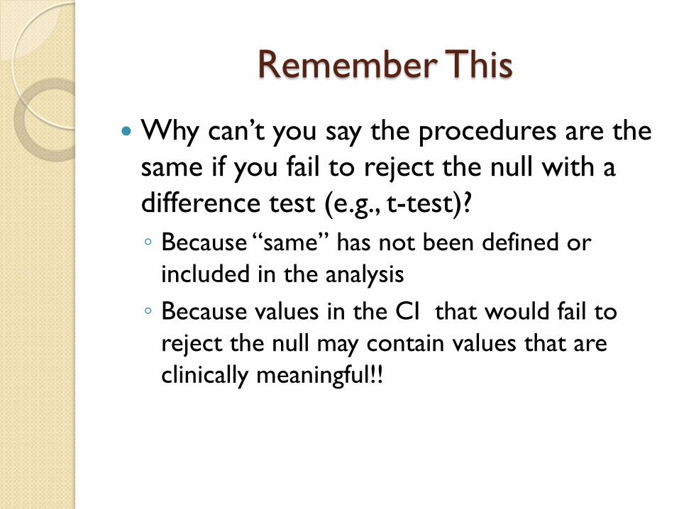
Remember This

Why can’t you say the procedures are the same if you fail to reject the null with a difference test (e.g., t-test)?◦ Because “same” has not been defined or

included in the analysis◦ Because values in the CI that would fail to

reject the null may contain values that are clinically meaningful!!

95% CI for Mean Difference Proc1 vs.

0 2 4 6

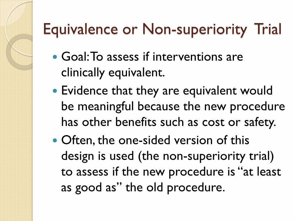
Equivalence or Non-superiority Trial

Goal: To assess if interventions are clinically equivalent.

Evidence that they are equivalent would be meaningful because the new procedure has other benefits such as cost or safety.

Often, the one-sided version of this design is used (the non-superiority trial) to assess if the new procedure is “at least as good as” the old procedure.

Equivalence Trial

Null Hypothesis: |Mean 1 – Mean 2| ≥ Γ (gamma),

a pre-specified threshold below which is “clinically meaningless”

Alternative Hypothesis: |Mean 1 – Mean 2| < Γ

Equivalence or Non-superiority Trial

Power Analysis: Need to specific the biggest difference that would be clinically meaningless (Effect Size).

Using the example from above, if 5 SOM points is clinically meaningful, then presumably the threshold for clinically meaningless is less than 5.

Lets say that we decide that a difference of 2 SOM points is basically meaningless. So the null hypothesis is the |Mean 1 – Mean 2| ≥ 2.

Power Analysis

sample sizes of 226 in the first group and 226 in the second group achieve 80% power at a 0.10 one-sided significance level. (overall alpha = 0.05)

ResultsMean (SD) of Procedure 1 55.2 (9.7) Mean (SD) of Procedure 2 55.6 (9.2)

90 percent confidence interval for the mean difference: [-1.9 to 1.0]

TOST procedure (two one sided tests): p = 0.04

Dependent or Clustered Data Statistics 101 only covers methods that have a

strong assumption of independent errors (e.g., ANOVA, independent sample t-tests, OLS regression).

Many of our data and questions have dependencies that require other less familiar methods.

Dependent, non-independent, correlated, nested, clustered errors…. All the same thing.

Goals• Be able to recognize dependences in

data.• Patients within clinics• Repeated measures on units• Longitudinal data

• Understand dangers of ignoring this issue

• Highlight common bad methods• Provide a basic orientation to one

statistical framework for handling dependencies: Mixed-effects regression

Common Data Structures

Multi-Level Organizational Data◦ Patients within providers within facilities

C3C1 C2 C6C4 C5

PT1_3 PTN_3 PT1_5 PTN_5

C3 C5

45

67

89

10

clinic

scor

e

C3 C5

-3-2

-10

12

3

clinic

erro

rs

Common Data Structures

Repeated measures per unit◦ Several BPs per person at each assessment

and/or over time◦ Several assays per culture

SBP

Pat

ient

2

5

1

6

3

4

40 60 80 100

Common Data Structures

Repeated-measures on individuals over time◦ Monthly measurement of disease status

Y

Time

Common Data Structures

Both within person and within organization clustering◦ RCT where providers are the unit of

randomization◦ Outcomes are patient-level trajectories

◦ Site\provider\patient\BP

The Problem

Common statistical tools have no good way of dealing with multi-level details (correlated errors, sample size, variances)◦ OLS Regression◦ ANOVA◦ t-tests

It matters – failing to attend to these details can give very wrong results.

Old (and usually bad) Solutions

To aggregate or disaggregate data to one level and apply familiar statistical models.

Example Study: What are the clinic characteristics

(e.g., co-located social work service) that influence patient outcomes?◦ Sample is 700 patients in 20 clinics

Bad Solutions:

◦ Force all information to the patient-level◦ Force all information to the clinic-level

Usual Methods Get This WrongPatient ID Clinic ID Patient

OutcomeClinic Factor

1 1 12 0

2 1 11 0

3 1 13 0

4 1 7 0

5 1 6 0

6 2 2 1

7 2 12 1

8 2 11 1

9 2 13 1

10 2 7 1

11 3 6 0

etc etc etc etc

Forcing Information to the Patient-level

Confounds patient and clinic sample sizes Radically reduces the SE of parameter

estimates Leads to more null-hypothesis rejection

and inappropriately narrow CIs

Force all information to the Clinic-level

Site ID Patient Outcome Site Factor

1 7.5 0

2 5.6 1

3 8.2 0

4 9.7 1

Force all information to the Clinic-level

Lose power Lose information about within clinic

variability and sample size

Compare Methods OLS regression on 700 observations

OLS regression on 20 observations

Mixed-Effects Regression Test t statistic◦ 10.0, 3.2, 3.5

Variance Partitioning in Regular Regression

0 12

( ) + where ~ (0, )

i i i

i

y ClinicCharacteristic ee N

β β

σ

= +

Variance Partitioning in Mixed –Effects (Multi-Level) Regression

ij 0j 01 j j ij

2 2j μ i e

y = + (CC) + μ + e

where μ ~ N(0, σ ), e ~ N(0, σ )

γ γ

Mixed Effects Regression (HLM, mixed models, random effects models, etc.)

Keeps track of multi-level details and allows for dependencies.

Generalized versions (logistic, Cox, count) Handles unbalanced data and variable

assessment schedules, all cases can be included Implemented in most major packages Other strategies/models are available that

handle some of these details (robust/shrunken SE; fixed effects models; GEE).

Mixed Effects Regression Address single-level questions while accounting

for dependencies at other levels. Do patients who have a particular

procedure have better outcomes? Test interesting and important multi-level

(cross-level) hypotheses.◦ Does surgical setting (e.g., academic, private

group practice) affect patient outcomes?

Example 2

Unit level question with multiple observations per unit

What is the mean SBP for a sample patients?

How much variability is there between patients?

Example and data modified from Pinheiro & Bates “Rail” example.

SBP

Pat

ient

2

5

1

6

3

4

40 60 80 100

Approach 1lm(formula = SBP ~ 1, data = SBP)

Coefficients:

Estimate Std. Error t value Pr(>|t|)

(Intercept) 66.500 5.573 11.93 1.10e-09 ***

---

Residual standard error: 23.65 on 17 degrees of freedom

95% CI of mean = [54.7, 78.2]

Gets the sample size wrong, SE too small, does not distinguish between and within person variance

2 5 1 6 3 4

-40

-20

020

Patient

erro

rs

Approach 2 lm(formula = SBP ~ 1, data = SBPAggregatedData)

Coefficients:

Estimate Std. Error t value Pr(>|t|)

(Intercept) 66.50 10.17 6.538 0.00125 **

Residual standard error: 24.91 on 5 degrees of freedom

95% CI of mean = [54.7, 78.2] in Approach 1

Now [40.3, 92.6]

Solves correlated error problem but throws away data about within person variability.

Approach 3Mod4<-lme(SBP~1, random = ~1|Patient, data = SBP)

Random effects:

Formula: ~1 | Patient

(Intercept) Residual

StdDev: 24.80547 4.020779

ICC = .97

Fixed effects: SBP ~ 1

Value Std.Error DF t-value p-value

(Intercept) 66.5 10.17104 12 6.538173 0

Number of Observations: 18

Number of Groups: 6

Compare the CIs 95% CI of mean = [54.7, 78.2] in Approach 1

[40.3, 92.6] in Approach 2

[46.6, 86.4] in Approach 3

Approach 1 overestimates precision

Approach 2 underestimates precision

Approach 3 is just right

Example from This Week!

What are the factors that are associated with surgeons requesting GA for CTR?

glm(formula = ga ~ c.age + gender.factor + race + marital.rec + serviceConnect.factor + asaClass.factor, family = binomial, data = x)

Deviance Residuals: Min 1Q Median 3Q Max

-0.8106 -0.5965 -0.5631 -0.5228 2.1832

Coefficients:Estimate Std. Error z value Pr(>|z|)

(Intercept) -1.945842 0.196584 -9.898 < 2e-16 ***c.age -0.008454 0.002006 -4.215 2.50e-05 ***gender.factorM -0.152158 0.070464 -2.159 0.0308 * raceNon-Hispanic Black 0.297721 0.061571 4.835 1.33e-06 ***raceOther minority 0.061751 0.081951 0.754 0.4511 marital.recDivorced/separated 0.058132 0.050464 1.152 0.2493 marital.recNEVER MARRIED 0.067604 0.082320 0.821 0.4115 marital.recSingle or widow/widower -0.089112 0.109629 -0.813 0.4163 serviceConnect.factorNSC or <50% -0.071935 0.045883 -1.568 0.1169 serviceConnect.factorOther -0.189297 0.200324 -0.945 0.3447 asaClass.factor2 0.260787 0.185702 1.404 0.1602 asaClass.factor3 0.417518 0.186095 2.244 0.0249 * asaClass.factor4 0.578912 0.230124 2.516 0.0119 * ---Signif. codes: 0 ‘***’ 0.001 ‘**’ 0.01 ‘*’ 0.05 ‘.’ 0.1 ‘ ’ 1

Generalized linear mixed model fit by maximum likelihood (Laplace Approximation) ['glmerMod']Family: binomial ( logit )Formula: ga ~ c.age + gender.factor + race + marital.rec + serviceConnect.factor +

asaClass.factor + (1 | sta3n.factor/surgeon.factor)

Random effects:Groups Name Variance Std.Dev.surgeon.factor:sta3n.factor (Intercept) 1.904 1.380 sta3n.factor (Intercept) 3.121 1.767 Number of obs: 16053, groups: surgeon.factor:sta3n.factor, 785; sta3n.factor, 111

Fixed effects:Estimate Std. Error z value Pr(>|z|)

(Intercept) -2.658075 0.308538 -8.615 < 2e-16 ***c.age -0.013861 0.002591 -5.349 8.86e-08 ***gender.factorM -0.038550 0.089761 -0.429 0.668 raceNon-Hispanic Black 0.078207 0.083720 0.934 0.350 raceOther minority -0.157742 0.108698 -1.451 0.147 marital.recDivorced/separated 0.100191 0.063846 1.569 0.117 marital.recNEVER MARRIED 0.026475 0.104431 0.254 0.800 marital.recSingle or widow/widower -0.028766 0.136205 -0.211 0.833 serviceConnect.factorNSC or <50% 0.070086 0.058559 1.197 0.231 serviceConnect.factorOther -0.055370 0.254383 -0.218 0.828 asaClass.factor2 -0.019916 0.230841 -0.086 0.931 asaClass.factor3 0.149605 0.232928 0.642 0.521 asaClass.factor4 0.150451 0.291095 0.517 0.605 ---Signif. codes: 0 ‘***’ 0.001 ‘**’ 0.01 ‘*’ 0.05 ‘.’ 0.1 ‘ ’ 1

Suggested Resources for Learning About Mixed Effects Models Pinheiro, J., & Bates, D. (2000). Mixed Effects Models in S

and S-Plus. New York, NY: Springer. Raudenbush, S. W., & Bryk, A. S. (2001). Hierarchical Linear

Models : Applications and Data Analysis Methods (2nd ed.). Thousand Oaks, CA: Sage.

Singer, J. D., & Willett, J. B. (2003). Applied longitudinal data analysis: Modeling change and event occurrence. London: Oxford University Press.

Hox, J. J. () Applied Multilevel Analysis. http://www.fss.uu.nl/ms/jh/publist/amaboek.pdf

Fitzmaurice GM, Laird NM, Ware JH: Applied longitudinal analysis. John Wiley & Sons, New York; 2004.

Punch Line

Multi-level thinking is powerful and important conceptually and statistically

Need to use models that keep track of multi-level details◦ Sample size◦ Variance partition◦ Correlated errors

Unless you want to commit a lot of time to this, ask for help.

Time Allowing…

Power Analysis Alpha adjustments for multiple tests Parametric methods vs. alternatives

Thank [email protected]