Topics in Control of Nanopositioning Devices Thesis for the degree of Philosophiae Doctor Trondheim, November 2012 Norwegian University of Science and Technology Faculty of Information Technology, Mathematics and Electrical Engineering Department of Engineering Cybernetics Arnfinn Aas Eielsen

Welcome message from author
This document is posted to help you gain knowledge. Please leave a comment to let me know what you think about it! Share it to your friends and learn new things together.
Transcript

Topics in Control of Nanopositioning Devices
Thesis for the degree of Philosophiae Doctor
Trondheim, November 2012
Norwegian University of Science and TechnologyFaculty of Information Technology, Mathematics and Electrical EngineeringDepartment of Engineering Cybernetics
Arnfinn Aas Eielsen

NTNUNorwegian University of Science and Technology
Thesis for the degree of Philosophiae Doctor
Faculty of Information Technology, Mathematics and Electrical EngineeringDepartment of Engineering Cybernetics
© Arnfinn Aas Eielsen
ISBN 978-82-471-3949-3 (printed ver.)ISBN 978-82-471-3950-9 (electronic ver.)ISSN 1503-8181
ITK Report 2012-6-W
Doctoral theses at NTNU, 2012:315
Printed by NTNU-trykk

To my parents.


Summary
Nanopositioning concerns motion control with resolution down to atomic scale.Positioning devices with such a capability have applications in numerous areas inindustry and science. Examples include scanning probe microscopy, adaptive op-tics, hard disk drive systems, and the production and inspection of high-densitysemiconductor designs. Scanning probe microscopy is perhaps the most prominentexample, as it is a versatile tool, which can be used for imaging, metrology, andphysical manipulation. In imaging applications, the achievable resolution, or accu-racy, is the most important performance criterion. For metrology and manipulation,trueness is also of importance. Additionally, the maximum achievable throughput,or bandwidth, of nanopositioning systems is an important performance criterion,as it lays the foundation for fast measuring and manipulation of physical proper-ties; capturing processes at the time scale which they occur, reducing time and costrelated to metrology, and enabling fabrication of nanoscale features at an industrialscale.
Nanopostitioning devices ubiquitously use piezoelectric actuators, as such actu-ators enable fast and frictionless motion. Piezoelectric actuators are as such idealfor high resolution positioning tasks. Positioning devices utilizing piezoelectric ac-tuators typically exhibit lightly damped vibration modes, as well as hysteresis andcreep non-linearities. Lightly damped vibration modes limits the achievable band-width, and hysteresis and creep limits the trueness of such devices. In order toimprove bandwidth and trueness, these phenomena can be countered using feed-forward and feedback control.
Part I of this thesis presents an adaptive feed-forward technique to compensatefor the hysteresis non-linearity. It is based on the Coleman-Hodgdon model, andprovides an open-loop observer for the hysteretic behavior which can be used tolinearize the output of an actuator which exhibit hysteresis that can be modeledwith said model. The model provides a good description of hysteresis responses thatare symmetric, and the compensation method provides the best performance forstationary periodic reference trajectory signals. It is also pointed out that hysteresiscan be interpreted as an uncertain gain and an input disturbance, and as such,regular feedback control using high quality position sensors can also effectivelyreduce the effect of hysteresis if the bandwidth is sufficiently high, and if the controllaw is robust towards variation in low-frequency gain. The drawback is increasedposition noise, due to sensor noise being amplified and fed back into to the actuationsignal.
iii
Summary
Part II concerns so-called damping and tracking control, and presents severallow-order control schemes to improve bandwidth by damping lightly damped vi-bration modes, and by doing so, allowing for higher gain in the feedback controllaw. A practical tuning procedure is introduced in order to find optimal control lawparameters, using an flatness criterion for the complementary sensitivity function.The effect of quantization noise due to implementation on digital signal processingequipment is investigated, and a particular simple damping and tracking controllaw is introduced, which consists of an integrator and a low-pass filter. The low-pass filter can be implemented using the anti-aliasing and reconstruction filtersneeded when using digital signal processing equipment, and only the integratorneeds to be implemented digitally. The optimal tuning of this control structureturns out to limit the bandwidth of the anti-aliasing and reconstruction filters,and due to the limited bandwidth of the reconstruction filter, quantization noise iseffectively attenuated. This control scheme is then coupled with a repetitive con-trol scheme, which provides good tracking of periodic reference signals. A simpletime-delay with positive feedback is a model for any periodic signal with a fixedperiod, and the repetitive control scheme includes this model in the feedback path,and can thus null any exogenous periodic signal with that fixed period to the errorsignal, due to the internal model principle. A criterion for robust stability of thedamping and tracking control law combined with the repetitive control scheme ispresented, which ensures stability for a prescribed unstructured uncertainty incor-porating variable gain due to, among other factors, hysteresis, and high-frequencynon-modeled dynamics.
Part III discusses adaptive control for arbitrary reference trajectory signals.Instrumentation used in nanopositioning systems typically allow for output feed-back only, and the application of the standard framework for output feedback fordominantly linear systems, the model reference adaptive control scheme, is investi-gated. The model reference adaptive control scheme requires the usage of an onlineadaptive law in order to learn the parameter values of an uncertain model, and twocommon parameter identification schemes, the recursive least-squares method andthe extended Kalman filter, are assessed for their ability to learn the parameters ofa mass-spring-damper system using experimental data recorded using a nanoposi-tioning device with two different payload configurations in open-loop. The result isa special pre-filter, which is demonstrated to improve parameter convergence. Themodel reference adaptive control scheme is then assessed experimentally, and it isdemonstrated that a further refinement of the pre-filter is needed in order to obtainreasonable parameter convergence in closed-loop. An integral adaptive law is usedin this case, in order to improve the convergence rate of the parameter estimates.
The main contributions of the thesis are methods for feed-forward and feedbackcontrol that can achieve similar or better performance than existing methods, butwith lower complexity, which improves practical implementability.
iv

Contents
Summary iii
Contents v
Preface ix
1 Introduction 11.1 Nanopositioning . . . . . . . . . . . . . . . . . . . . . . . . . . . . 11.2 Instrumentation . . . . . . . . . . . . . . . . . . . . . . . . . . . . . 21.3 Control Schemes Survey . . . . . . . . . . . . . . . . . . . . . . . . 61.4 Topics of This Thesis . . . . . . . . . . . . . . . . . . . . . . . . . . 101.5 Publications . . . . . . . . . . . . . . . . . . . . . . . . . . . . . . . 12
I Feed-Forward Control of Hysteresis 15
2 Hysteresis Compensation 172.1 Introduction . . . . . . . . . . . . . . . . . . . . . . . . . . . . . . . 172.2 System Description & Modeling . . . . . . . . . . . . . . . . . . . . 182.3 Feed-Forward Tracking Control . . . . . . . . . . . . . . . . . . . . 212.4 Experimental Results & Discussion . . . . . . . . . . . . . . . . . . 232.5 Parameter Identification . . . . . . . . . . . . . . . . . . . . . . . . 262.6 Derivation of the Equivalent Coleman-Hodgdon Model . . . . . . . 282.7 Derivation of the Hysteresis Compensation Scheme . . . . . . . . . 302.8 Passivity of the Hysteresis Model . . . . . . . . . . . . . . . . . . . 312.9 Hysteresis as an Uncertain Gain & an Input Disturbance . . . . . . 322.10 Adding Integral Control . . . . . . . . . . . . . . . . . . . . . . . . 352.11 Trajectory Generation . . . . . . . . . . . . . . . . . . . . . . . . . 352.12 Conclusions . . . . . . . . . . . . . . . . . . . . . . . . . . . . . . . 36
II Damping & Tracking Control 39
3 Damping & Tracking Control Schemes for Nanopositioning 413.1 Introduction . . . . . . . . . . . . . . . . . . . . . . . . . . . . . . . 413.2 System Description & Modeling . . . . . . . . . . . . . . . . . . . . 42
v
Contents
3.3 Control Design . . . . . . . . . . . . . . . . . . . . . . . . . . . . . 473.4 Damping & Tracking Control Schemes . . . . . . . . . . . . . . . . 543.5 Experimental Results & Discussion . . . . . . . . . . . . . . . . . . 723.6 PI2 Anti-Windup Using Conditional Integrators . . . . . . . . . . . 743.7 Conclusions . . . . . . . . . . . . . . . . . . . . . . . . . . . . . . . 81
4 Robust Repetitive Control 834.1 Introduction . . . . . . . . . . . . . . . . . . . . . . . . . . . . . . . 834.2 System Description & Modeling . . . . . . . . . . . . . . . . . . . . 854.3 Control Structure . . . . . . . . . . . . . . . . . . . . . . . . . . . . 884.4 Control Scheme Tuning & Analysis . . . . . . . . . . . . . . . . . . 934.5 Experimental Results & Discussion . . . . . . . . . . . . . . . . . . 1044.6 Conclusions . . . . . . . . . . . . . . . . . . . . . . . . . . . . . . . 109
III Adaptive Control 111
5 Online Parameter Identification 1135.1 Introduction . . . . . . . . . . . . . . . . . . . . . . . . . . . . . . . 1135.2 System Description & Modeling . . . . . . . . . . . . . . . . . . . . 1145.3 Identification Schemes . . . . . . . . . . . . . . . . . . . . . . . . . 1185.4 Experiments . . . . . . . . . . . . . . . . . . . . . . . . . . . . . . . 1205.5 Results . . . . . . . . . . . . . . . . . . . . . . . . . . . . . . . . . . 1225.6 Discussion . . . . . . . . . . . . . . . . . . . . . . . . . . . . . . . . 1235.7 Conclusions . . . . . . . . . . . . . . . . . . . . . . . . . . . . . . . 126
6 Robust Adaptive Control 1296.1 Introduction . . . . . . . . . . . . . . . . . . . . . . . . . . . . . . . 1296.2 System Description & Modeling . . . . . . . . . . . . . . . . . . . . 1306.3 Model Reference Adaptive Control . . . . . . . . . . . . . . . . . . 1346.4 Design Choices . . . . . . . . . . . . . . . . . . . . . . . . . . . . . 1366.5 Experimental Results & Discussion . . . . . . . . . . . . . . . . . . 1416.6 Conclusions & Future Works . . . . . . . . . . . . . . . . . . . . . 143
Appendices 147
A Piezoelectric Transducers 149A.1 Piezoelectricity . . . . . . . . . . . . . . . . . . . . . . . . . . . . . 149A.2 Matrix Notation . . . . . . . . . . . . . . . . . . . . . . . . . . . . 154A.3 Stack Actuator Blocking Force . . . . . . . . . . . . . . . . . . . . 156A.4 Charge in Actuator Circuit . . . . . . . . . . . . . . . . . . . . . . 159A.5 One-Dimensional Transducers . . . . . . . . . . . . . . . . . . . . . 160
B Mechanical Vibrations 163B.1 Distributed-Parameter Structures . . . . . . . . . . . . . . . . . . . 163B.2 Lumped-Parameter Structures . . . . . . . . . . . . . . . . . . . . 169B.3 Some Facts About Second-Order Systems . . . . . . . . . . . . . . 173
vi
Contents
C Hysteresis & Creep Models 175C.1 Hysteresis . . . . . . . . . . . . . . . . . . . . . . . . . . . . . . . . 175C.2 The Duhem Model . . . . . . . . . . . . . . . . . . . . . . . . . . . 176C.3 The Preisach Model . . . . . . . . . . . . . . . . . . . . . . . . . . 177C.4 Creep Models . . . . . . . . . . . . . . . . . . . . . . . . . . . . . . 181
D Online Parameter Identification Schemes 183D.1 Recursive Least-Squares Method . . . . . . . . . . . . . . . . . . . 183D.2 Integral Adaptive Law . . . . . . . . . . . . . . . . . . . . . . . . . 185D.3 Extended Kalman Filter . . . . . . . . . . . . . . . . . . . . . . . . 185
E Model Reference Adaptive Control & Model Reference Control 189E.1 Model Reference Adaptive Control . . . . . . . . . . . . . . . . . . 189E.2 Model Reference Control . . . . . . . . . . . . . . . . . . . . . . . . 191
References 193
vii


Preface
This thesis is submitted in partial fulfillment of the requirements for the degree ofphilosophiae doctor (PhD) at the Norwegian University of Science and Technology(NTNU).
The work for this thesis has mainly been carried out at the Department ofEngineering Cybernetics, in the period from October 2008 to August 2012. Mysupervisor has been Prof. Jan Tommy Gravdahl, and my co-supervisors have beenProf. Kristin Ytterstad Pettersen, and Prof. Tomas Tybell.
Funding for the PhD position, as well as laboratory equipment and travel,has been provided by the Norwegian University of Science and Technology, theDepartment of Engineering Cybernetics, and the Research Council of Norway.
During this period I have had the privilege of two extended visits, to Prof. S. O.Reza Moheimani at the Laboratory for Dynamics and Control of Nano Systems andDr. Andrew J. Fleming at Centre for Complex Dynamic Systems and Control, bothat the University of Newcastle, Australia, as well as to Assoc. Prof. Kam K. Leangand his student Mr. Brian Kenton at the Mechanical Engineering Department atthe University of Nevada, Reno, USA. I am very grateful for their hospitality.
I am also grateful for the opportunity for some shorter visits. I visited Prof.Georg Schitter, which at the time was employed at the Delft Center for Systemsand Control at the Delft Technical University, the Netherlands, and his formerstudents Dr. Stephan Kuiper and Dr. Jan Roelf van Hulzen, I had a great tour ofLeiden University and some of the laboratory facilities there with Dr. Gertjan vanBaarle from Leiden Probe Microscopy BV, as well as a visit to Prof. ChristophAment and his former student Dr. Arvid Amthor at the Faculty of ComputerScience and Automation at the Ilmenau University of Technology, Germany.
I also had the pleasure of working with my good colleague for three years, Dr.Mernout Burger, now employed at the Delft University of Technology, as well asas Dr. Tomáš Polóni from the Slovak University of Technology in Bratislava, andProf. Tor Arne Johansen and Dr. Marialena Vagia at our department.
A special ‘thank you’ goes to the technical staff at our department, especiallyTerje Haugen, Per Inge Snildal, Stefano Bertelli, John Olav Horrigmo, TorkelHansen and Rune Mellingseter, who provided invaluable aid in building, operating,and maintaining the lab equipment.
I would also like to thank all my fellow PhD students at the department, presentand former. Christian, Christoph, Serge, Øyvind, Anders, Milan, Giancarlo, Esten,Espen, Aleksander, Walter, Mark, Mladen, and all the rest. In total it has been asizable amount of beer, cake, and bad jokes.
ix

Preface
Lastly, I would like to thank my parents, Anne-Kari and Steinar, for all theirsupport and help through four eventful years.
Arnfinn Aas EielsenTrondheim, November 2012
x

Chapter 1
Introduction
1.1 Nanopositioning
Nanopositioning is a neologism used to refer to positioning devices that have thecapability to generate mechanical displacements down to atomic scale resolution.Positioning devices with such a capability have applications in numerous areasin science and industry. Perhaps the most prominent example of motion controlwith this type of resolution requirement is found in the field of scanning probemicroscopy [186]. Other application areas of high-resolution motion control can befound in adaptive optics [217], in modern hard disk drive systems [4], and in theproduction and inspection of high-density semiconductor designs [99].
Scanning probe microscopy is a collective term for a vast array of mechanicalsurface interrogation and manipulation techniques, which can be done in either avacuum, air, or a liquid. Common to all the techniques is the need to position aphysical probe with extremely high resolution.
In modern scanning probe microscopy instruments, this is typically done byusing a lateral positioning mechanism to allow positioning of a point on a sampleunder a separate, vertically actuated probe. The probe, typically attached to thetip of a small cantilever, can then interact with the surface at that point. Due to theversatility of scanning probe microscopy instruments, it has become an importanttool for surface imaging, metrology, and physical manipulation at the nanoscale.
The origin of the field of scanning probe microscopy, appears to be the in-vention of the Topografiner [228]. The Topografiner measured the field emissioncurrent between a probe and the surface of an electrically conducting sample, andused it as a distance measurement. By scanning the surface in a raster patternit could then be used to build a topographic image of the surface with nanoscaleresolution. Since then, notable extensions of the operating principles introducedby the Topografiner, include the scanning tunneling microscope [30], resolving fea-tures with atomic resolution [31], the atomic force microscope [32], manipulationof single atoms [72], and so-called video-rate imaging [11].
Imaging applications of scanning probe microscopy aim at collecting qualita-tive information about the sample surface. Examples of such information can bethe topology, various optical, electrical, and magnetic properties, and mechanical
1

1. Introduction
properties, such as friction and roughness. In scanning probe microscopy, theseproperties are measured using specialized probes and various types of modulationof the probe.
For imaging, the resolution, or precision, is one of the most important perfor-mance specifications. This is because it is of importance to detect the smallestpossible features. For metrology applications, often the same surface informationis sought, but in this context, the trueness of the measured quantities is also ofimportance. The trueness accounts for the closeness between the measured meanvalue and the true value of the physical property. Trueness is also important formanipulation applications, in order to repeatedly produce features according tospecifications.
For a survey of scanning probe microscopy imaging, metrology, and manipula-tion applications and techniques, see [28, 41, 52, 59, 189, 205].
For applications of scanning probe microscopy, one of the main challenges is toincrease the bandwidth, or throughput, for both measurement and manipulation.Higher throughput is needed to, e.g., reduce the amount of time used to generate aset of measurements, capture the time evolution of physical processes, reduce costsrelated to metrology in industrial processes, and to enable fabrication of nanoscalefeatures at an industrial scale [44, 58, 97, 191, 209].
1.2 Instrumentation
1.2.1 Positioning Devices
The positioning devices used in scanning probe microscopy systems span fromlong-range voice-coil actuated devices [8, 19, 149] to shorter range devices usingpiezoelectric actuators [29, 30, 120, 131, 183, 184, 200].
The mechanical design of nanopositioning stages provides fundamental limita-tions to the achievable performance for any control scheme. The main performancespecifications for nanopositioning stages are the range and the dominant vibra-tion mode, which preferably is the first vibration mode. The resonant frequencyof the dominant vibration mode is usually the limiting factor for the attainablebandwidth. One reason is that it can be difficult to control higher-order vibrationmodes, as they might be practically uncontrollable; having mode shapes and direc-tions that are weakly coupled with the mounted actuator. Another reason is thatthe control signal amplitude and the amount of power required to drive the systemabove the dominant resonance can become prohibitive, as driving amplifiers willeventually saturate [83, 137].
As a rule of thumb, there is an inverse relationship between range and band-width, thus to achieve high bandwidth, the range is usually limited [44]. The band-width can roughly be estimated to be equal to the frequency of the dominantvibration mode of the mechanical structure.
The Topografiner and the scanning tunneling microscope used a tripod configu-ration of piezoelectric stack actuators [30, 228]. The piezoelectric tube actuator waslater introduced as an improvement over this design [29]. Compared to the tripodactuator, the tube actuator increased the achievable range, it had a higher domi-nant resonant frequency, it experienced less influence from environmental vibration
2

1.2. Instrumentation
disturbances, it had smaller physical dimensions, a simpler design which was easierto manufacture and assemble, and it was less susceptible to thermal drift. As such,it is perhaps the most proliferate mechanism in the first generations of scanningprobe microscopy systems [5]. A comprehensive analytical model for piezoelectrictube actuators is presented in [74], and a finite-element model is discussed in [147].
Newer device designs use flexure guided mechanisms [120, 131, 200, 223, 225],which provide further improvements; as flexure guided mechanisms allow for longerrange, a higher dominant resonant frequency, and experience less cross-coupling andnon-linearity in the actuation directions. The main disadvantages are a less com-pact design, and in some cases a more elaborate manufacturing process, sometimesrequiring specialized machining tools, such as a wire electrical discharge machine.
Voice coil actuators typically allow for nanopositioning devices with longerrange, compared to devices using piezoelectric actuators [19, 51, 149]. These devicescan then accommodate for large samples and large surface features. Depending onthe design, these devices generally have a much lower bandwidth than devices usingpiezoelectric actuators. The designs in [19, 51] uses flexures to guide the motion,but for longer range motion, guides in the form of bearings is used [149], whichadds the additional problem of friction [8].
1.2.2 Positioning Devices using Piezoelectric Actuators
As piezoelectric actuators can produce large forces, provide frictionless motion,and the resolution is only limited by instrumentation noise, they are ideal for high-bandwidth, high-resolution positioning. As such, they are ubiquitous in nanoposi-tioning devices. An introduction to standard piezoelectric transducer modeling isfound in Appendix A.
Mechanical vibrations
A positioning device utilizing piezoelectric actuators typically exhibits lightly dampedvibration modes. This is a disadvantage, as it limits the usable bandwidth becausereference signals with high frequency components will excite the vibration modes,prohibiting accurate positioning. It also makes the device susceptible to environ-mental vibration disturbances, such as sound and floor vibrations. An introductionto standard mechanical vibration modeling is found in Appendix B.
Hysteresis and creep
The hysteresis and creep non-linearities in piezoelectric actuators is an additionalchallenge. These are loss phenomena that prevent the system from having a linearresponse, introducing bounded input disturbances dependent on the driving voltagesignal.
Creep is mainly a problem when applying feed-forward control for low-frequencyand static positioning, as the phenomenon can be observed as a slow creepingmotion after applying, e.g., a voltage step to the piezoelectric actuator. An exampleof this kind of response is shown in Fig. 1.1.
3

1. Introduction
0 2 4 6 8 10 12 14 16 18 205.5
5.6
5.7
5.8
5.9
6
6.1
6.2
6.3
6.4
6.5
Time (s)
Dis
plac
emen
t (μm
)
Figure 1.1: Piezoelectric actuator creep response to a voltage step.
Hysteresis is a problem for any time-varying reference signal tracking, becauseit introduces a rate-independent lag when applying a voltage signal to the actuator,and consequently to the resulting displacement of the piezoelectric transducer. Thislag can be interpreted as a bounded input disturbance to the system. Examples ofhysteretic responses to sinusoidal voltage signals are shown in Fig. 1.2a.
An introduction to common hysteresis and creep models is found in Appendix C.
Parameter and model uncertainty
The mechanical vibration dynamics of a point on a positioning device structurecan be modeled with very high accuracy using linear ordinary differential equationsfor specific operating points. However, there are several sources of parameter andmodel uncertainty.
Hysteresis, in addition to introducing an input disturbance, change the effectivegain of the actuator depending on the amplitude and frequency of the driving volt-age signal [107, 171]. This is illustrated in Fig. 1.2b. The piezoelectric actuator gainis also dependent on temperature, and reduces over time due to depolarization [25].
In addition, users typically need to position payloads of various masses, thusresonant frequencies and the effective gain of the mechanical structure change as aresult [140].
The observed dynamic response is also affected by how well the sensors canbe co-located with the actuators [172]. Also, the dominant vibration mode of thepositioning device dynamics is usually designed to have a shape that providesmotion in a desired direction, and higher-order vibration modes are likely to have
4

1.2. Instrumentation
Voltage (V)
Dis
plac
emen
t (μm
)
(a) Ensemble of measured hysteresis responsesfor different voltage signal amplitudes.
Voltage (V)
Dis
plac
emen
t (μm
)
(b) Change in average linear gain for low ampli-tude voltage signals and high amplitude voltagesignals.
Figure 1.2: Piezoelectric actuator hysteretic responses to sinusoidal voltage signals.
shapes and directions that will make them difficult to control using the mountedactuator. Thus, the model structure might be uncertain and it will have practicallyuncontrollable modes.
1.2.3 High-Resolution Sensors
To enable high-resolution motion control, high-resolution sensors are necessary.They are needed for system identification when utilizing feed-forward control, andthe performance of the sensor determines the precision and trueness achievablewhen using feedback control.
The noise specifications for a sensor is in general much stricter when appliedin feedback control, as the noise will be fed back to the input and will increasethe overall noise level in the system. For system identification, noise is of lessimportance, and can then often be reduced substantially by averaging.
The most common types of sensors found in nanopositioning devices are in-ductive probes [49], capacitive probes [78, 85], piezoelectric transducers [78, 81,84, 158], strain gauges [81, 192, 195], linear variable differential transformers [188],optical linear encoders [20, 131], and the Michelson interferometer [149]. Verticalcontrol of the probe in modern scanning probe microscopy instruments is almostexclusively done using an optical lever and a charge-coupled device [5].
System identification for the dynamic models is often done using displacementsensors and dynamic signal analyzer instruments, applying swept-sine or broad-band noise excitation signals. The first generations of scanning probe microscopyinstruments did not have displacement sensors for the lateral motion, but it is possi-ble in some circumstances to perform system identification for the lateral dynamicsusing vertical measurements from the probe [39, 43].
5

1. Introduction
1.2.4 The Signal Chain
The instrumentation dynamics of the components in the signal chain of the controlsystem should also be considered. The positioning device response will be influ-enced by the dynamics, saturation limits, and time-delays of amplifiers, sensors,anti-aliasing and reconstruction filters, as well as digital-to-analog and analog-to-digital converters. Some of these components exhibit significant non-linear re-sponses which can introduce systematic errors and noise. Typical examples includebad calibration of measurement instruments, which measurement principles exhibita non-linear characteristic, and noise due to sampling, quantization, and limitednumeric representation precision. These are general instrumentation and measure-ment limitations, and an introduction can be found in [163].
The implementation of the control laws can typically be done using digital signalprocessing equipment, or analog circuit elements. Digital control is the norm formost modern control systems [9], although the control systems for early scanningprobe microscopy instruments was realized using traditional analog operationalamplifier circuits [130].
Microprocessors or microcontrollers for high-bandwidth digital control is lim-ited by the attainable closed-loop sampling frequency. As a rule of thumb, themaximum practical closed-loop sampling frequency for digital signal processing us-ing microprocessors or microcontrollers is around 100 kHz. This excludes feedbackcontrol for very high bandwidth mechanical systems [191].
In order to increase the sampling frequency, field-programmable gate arrays(FPGA) can be used [120, 128, 184]. Field-programmable analog arrays (FPAA) isan analog alternative to FPGAs, and allows for fairly high-order control laws to beimplemented using analog circuit elements, and thus avoids sampling and allowsfor high-bandwidth control [129, 190, 199]. Regular operational amplifier circuitscan also be used for high-bandwidth control [78, 85].
The noise performance of a digital control system is limited by the noise floordetermined by both sampling frequency and quantization unit [145, 175, 220]. Thisdoes not seem to be discussed much in literature pertaining to scanning probemicroscopy.
1.2.5 The Environment
Imaging with atomic resolution puts very high requirements on the environmentalconditions in which an instrument operates, even though enabling instrumentationwith sufficient performance is readily available. This includes suppressing mechani-cal vibration noise from the environment, such as floor vibrations or sound, as wellas controlling ambient conditions, such at the temperature and humidity. Some-times vacuum or special atmospheric conditions are necessary, as sample surfacescan oxidize, or meniscus layers can form [41, 130, 229].
1.3 Control Schemes Survey
Motion control for nanopositioning devices appears to be a well-researched field.The literature regarding scanning probe microscopy appear to be coarsely divided
6
1.3. Control Schemes Survey
into research related to vertical and lateral positioning. For scanning probe mi-croscopy, both vertical and lateral positioning is necessary.
Vertical positioning is often coupled with a specific surface measurement or ma-nipulation technique [124]. For imaging applications, two common surface measure-ment techniques are the so-called contact mode and intermittent contact mode [5,186]. In both these cases, when applying feedback control, the control objective isto enforce a constant distance from the surface, treating the surface topology as adisturbance signal. In contact mode, the probe is dragged with constant interactionforce over the sample, where the force exerted on the surface through the probe isdue to the deflection of the cantilever. In intermittent contact mode the cantileveroscillates with a constant amplitude, and the interaction force determines the am-plitude. One of the main challenges for the control system design is therefore toprovide high-bandwidth control to suppress arbitrary disturbance signals, in orderto maintain a constant force or a constant oscillation amplitude.
For lateral positioning, the control objective is to provide accurate referencetrajectory tracking. The trajectory is often periodic, such as a triangle-wave signal,in order to produce the raster pattern needed in imaging applications. Many controlschemes for lateral positioning are therefore geared towards providing accuratetracking of such signals.
1.3.1 Feed-Forward Control
Inversion techniques
Feed-forward motion control can provide very good tracking results, if accurateand invertible models can be found for the system to be controlled. For stable,minimum phase linear systems it is especially straight forward, as it is in princi-ple possible to obtain perfect tracking by inverting the model of the system andby applying a sufficiently smooth reference trajectory. In the first generations ofscanning probe microscopy instruments, feed-forward control was used for lateralpositioning. The control signal was then generated simply by using a proportionalreference signal based on the DC-gains of the system, which did not provide anycompensation of creep, hysteresis, and mechanical vibrations [44]. This is sufficientfor low-bandwidth reference trajectories and imaging, where artifacts due to creepand hysteresis can be removed in image post-processing [20]. However, very goodtracking performance can be achieved for positioning devices using piezoelectricactuators when utilizing feed-forward control, when combining inverse models ofthe hysteresis, creep, and the mechanical vibration dynamics [50, 137, 177].
There are several examples of applying the inverse model of the mechanicalvibration dynamics to reduce motion-induced vibrations [48, 49, 123, 140, 193,197, 213, 230]. Some of these methods incorporate various optimization methodsin order to deal with parameter and model uncertainty, non-minimum phase zeros,to limit the control effort, and to handle only partially known reference signals.
Feed-forward inversion and linearization of hysteresis is most often done usingthe Preisach model [50, 212], or the Prandtl-Ishlinskii model [116, 159]. Anotherclass of hysteresis models, called Duhem models, have found some use, such asin [154], where a static map derived from the Coleman-Hodgdon equations is used.
7

1. Introduction
Feed-forward inversion of creep has also been investigated, using either staticmaps or linear ordinary differential equations [50, 116, 117, 159].
Trajectory generation
Another approach to reduce motion induced vibrations, is input shaping, whereinstead of using the plant inverse, the reference signal is chosen or modified in amanner which avoids excitation of lightly damped vibration modes. In this case,information about the mechanical vibration dynamics can be used either to reducethe frequency content of the reference signal, or to shape it to use the dynamicresponse of the positioner to good effect. Some examples are found in [83, 200].Work has also been done in order to reduce dynamic excitation by using sinusoidalscanning [22, 108, 216], and to use variable resolution in order to reduce the amountof time needed to cover a sample [10, 40].
1.3.2 Feedback Control
Feedback control can provide better tracking performance when combined withfeed-forward control, since feedback control reduces the sensitivity to unknowndisturbances and plant uncertainties for the controlled system. The main disad-vantage is the increased noise level due to sensor noise feedback.
Model-based control
Modern model-based control for output feedback on linear systems is commonlydone within the H∞-synthesis framework. It is perhaps the most practical frame-work for synthesizing robust control laws for arbitrary linear systems, as it guar-antees a solution to the control design problem by convex optimization [206]. Assuch, one would expect that control laws based on H∞-synthesis to be extensivelyexplored for nanopositioning systems, and several results can be found in the liter-ature [138, 187, 188, 192, 192, 194, 196, 198, 201, 211, 226]. Polynomial based, orpole-placement, control [94, 111] has also found some use [14]. Other model-basedcontrol schemes, such as the linear-quadratic-gaussian regulator [94], or model ref-erence control [94, 111], does not seem to have been applied to nanopositioningsystems. However, such control schemes can be seen as a subset of control schemesderived using H∞ or H2-synthesis.
Fixed-order, fixed-structure control
Traditional feedback control is often considered to be concerned with the appli-cation and tuning of the proportional–integral–derivative (PID) control law [17].For scanning probe microscopy systems, it is the standard choice for vertical con-trol [5, 194]. For lateral control in later generations scanning probe microscopysystems, proportional–double-integral–derivative (PIID) control laws and variantsthereof seem to be common, where double integral action is sometimes used toobtain asymptotic tracking of the flanks of a triangle signal, due to the internalmodel principle [20]. In order to increase the bandwidth and asymptotic trackingperformance for these systems, the control laws have sometimes been augmented
8

1.3. Control Schemes Survey
with notch filters, feed-forward control, and by using limited derivative and integralaction, also known as lead-lag control [6, 20, 75, 148, 187, 188, 194, 211, 231].
Since lightly damped vibration modes is the main problem for high-bandwidthtracking control, the sensitivity due to these modes can be reduced by using theactuator to increase the damping in the structure.
There exist several control schemes for introducing damping in active struc-tures. These include fixed-structure, low-order control laws such as positive posi-tion feedback [76], integral force feedback [174], passive shunt-damping [96], res-onant control [170] and integral resonant control [13]. For co-located sensors andactuators, many of the control laws have some good robustness and stability prop-erties due to positive-realness or negative-imaginariness for certain input-outputpairs [166]. A few damping control schemes using displacement feedback combinedwith feed-forward control have been investigated in [15, 26, 179, 202].
Piezoelectric actuators, or transducers, have a so-called self-sensing property,since any piezoelectric transducer can be used both for actuation and for sensing.The production of charge when a stress is applied is called the direct piezoelectriceffect, and the production of strain when an electric field is applied is called theconverse piezoelectric effect. By using the charge produced when operating theactuator, damping can be introduced without additional sensors [12, 82, 127]. Themain advantage of this technique is that there is very little, or no, increase in noisedue to sensor noise feedback.
By using so-called damping and tracking control schemes, reference trackingperformance can be further improved. This is done by coupling a damping con-trol scheme with an integral control law [14, 78, 85]. The main reason for theincreased performance is that a reduction of the dominant resonant peak of thesystem leads to an increased gain margin, enabling much higher gain to be used forthe disturbance-rejecting integral control law [78]. Due to the increased disturbancerejection, the adverse effects of creep and hysteresis can be reduced significantly.Environmental and other disturbances should also be reduced.
1.3.3 Other Approaches
Learning-type control
In many applications of nanopositioning devices, reference trajectories and distur-bances are periodic, or repetitive. This includes, e.g., tracking of raster patterns,producing a series of identical features in a manufacturing process, or measuringsurfaces with regularities in the topography.
Iterative learning control is a method that attempts to use the error signalproduced by successive periods of a reference signal to produce a feed-forwardcontrol signal that will invert the dynamic response of a systems, and cancel anydeterministic disturbances [35, 160]. There are several examples of the methodbeing applied to nanopositioning systems [36, 43, 101, 103, 122, 135, 141, 214,221]. In many of these cases, the method can provide practically perfect referencetracking.
Repetitive control is another control scheme that is tailored to provide smallerrors when using periodic reference signals, or in the presence of periodic distur-
9

1. Introduction
bances. It is based on the internal model principle, and thus operates by embeddinga model of periodic signals in the control loop [98]. Due to the internal model princi-ple, any exogenous signal that corresponds to the embedded model will be thereforebe nulled in the error signal. Examples of applications to nanopositioning systemsare found in [16, 155, 156].
Adaptive least mean squares filtering is also a technique that has also beeninvestigated for use on a nanopositioning device when applying periodic referencetrajectories [77].
Dual-stage actuation
In order to combine long range with high bandwidth, the principle of dual-stageactuation can be used. When using this technique, the mechanical system is mod-ified to use a high-bandwidth short-range actuator attached to a low-bandwidthlong-range actuator. The control schemes applied to these systems are often exten-sions to the ones already mentioned, such as damping and tracking control laws,and schemes derived using H∞-synthesis. Some examples of dual-stage actuationcan be found in [79, 105, 121, 128, 199].
Charge drive
With regards to the hysteresis in piezoelectric actuators, it is known that it appearsbetween applied voltage and induced charge [161]. By using a transconductance am-plifier, or charge drive, rather than a voltage amplifier, the hysteresis can effectivelybe eliminated [80, 118, 125].
Non-linear control
The vast majority of feedback control schemes in the literature are linear, likelydue to the fact that the dynamics of nanopositioning devices is dominantly linearand open-loop stable. Non-linear feed-forward schemes are found in the form ofthe hysteresis and creep compensation schemes already discussed. There are someexamples of classic non-linear feedback schemes applied to nanopositioning devices,in the form of sliding mode control [21, 61, 142].
1.4 Topics of This Thesis
The thesis is divided in three parts. Each part is concerned with a particular topicin control theory, and its application to nanopositioning devices. In this Section,the objectives and rationale for the work behind this thesis will first be presented,followed by a short discussion of the three parts.
1.4.1 Objectives and Rationale
The overall objective for the thesis work was to investigate and develop controlschemes for accurate trajectory tracking for nanopositioning devices, focussing
10

1.4. Topics of This Thesis
on practical and implementable methods, as well as verification of the methodsthrough physical experiments.
It was therefore necessary to assemble laboratory facilities to experimentallyassess the performance of motion control schemes applied to nanopositioning de-vices. The main guideline for acquiring laboratory equipment was that it shouldpreferably be generic and readily available from commercial manufacturers. It wasa goal that the laboratory set-up should resemble, as much as possible, a standardinstrumentation set-up for motion control. It was not a goal to aim for nanometeraccuracy or extremely high bandwidth, but rather have equipment that exhibitedthe main characteristics for devices used in nanopositioning applications. As such,it should be sufficient to verify the general operating principles for any developedmethods for motion control.
By the survey of the current literature on the subject of nanopositioning, it isapparent that it is well researched, and many approaches for control have beenproposed, experimentally verified, and found to be performing well. In the contextof nanopositioning devices, applied control theory can broadly be categorized intofeed-forward control, standard feedback control using linear filters, and adaptive,or learning, control. Here, feed-forward control chiefly deals with linear model in-version and inverse hysteresis operators, feedback control is most often done usingH∞-synthesis or a combination of damping and tracking control laws, and adap-tive control is done for periodic signals using iterative learning control, or similartechniques.
A common characteristic for inverse hysteresis operators, iterative learning con-trol, and control laws found using H∞-synthesis, is that the schemes yield goodresults, but can be of high order and computationally demanding. Iterative learningcontrol is also limited to tracking of periodic reference signals. This may limit theapplicability as implementation may require specialized numerical tools, fast digi-tal signal processing equipment, and an analog implementation can be practicallydifficult or impossible. It is noticeable from the current literature that there is littlediscussion on quantization noise, although control laws implemented using modernanalog circuit elements will provide superior noise performance compared to a dig-ital implementation. Control schemes that are suitable for analog implementationare the low-order damping and tracking schemes, but many of these schemes lacktools for systematic tuning.
The above assessment of the state of the art in the field of nanopositioninghas therefore motivated the investigation of control methods that are simpler withregards to implementation, but will produce similar performance to what has al-ready been done. The resulting work concerns hysteresis compensation (inversion),low-order damping and tracking control laws, robust low-order repetitive control,and robust adaptive control for arbitrary reference signals.
1.4.2 Part I – Feed-Forward Control of Hysteresis
This part contains Chapter 2, which presents a simple adaptive hysteresis com-pensation scheme. It is based on the material presented in [66, 69], but includesmore extensive analysis and discussion on the method, trajectory generation, the
11

1. Introduction
hysteresis phenomenon, and how to couple the method with an integral controllaw.
1.4.3 Part II – Damping & Tracking Control
Several low-order damping and tracking control schemes are presented and dis-cussed, as well as a repetitive control scheme for periodic reference trajectory track-ing. It is based material found in [63] concerning passive shunt damping, materialfound in [67] concerning optimal tuning of a modified proportional-integral (PI)control laws and anti-windup when using a proportional-double-integral (PI2) con-trol law, material found in [65, 71] concerning the implementation and tuning of allthe presented control schemes, as well as material found in [70] concerning robustrepetitive control.
Chapter 3 presents three damping and tracking control schemes already foundin the literature, as well as three control schemes based on passive shunt damping,a modified integral control law, and model reference control (MRC). A tuning pro-cedure for all the control schemes except the MRC scheme is presented. Extensiveanalysis of the different control schemes is also presented.
Chapter 4 presents a robust low-order approach to repetitive control for nanopo-sitioning, based partially on the modified integral control law from Chapter 3.
1.4.4 Part III – Adaptive Control
This part concerns adaptive control for arbitrary reference trajectories, using stan-dard adaptive control theory in the form of model reference adaptive control(MRAC). Chapter 5 is based on the material found in [68, 168, 169] concerning ex-perimental parameter identification for a nanopositioning device, and Chapter 6 isbased on material in [64] concerning implementation issues for a standard MRACapplied to a nanopositioning device. The work is mainly focussed on techniquesfor obtaining parameter convergence, and it is demonstrated experimentally thata pre-filter is needed to order to achieve this, both in open-loop and closed-loop.
1.4.5 Appendices
The appendices included are a collation of the standard theory on piezoelectricity,mechanical vibrations, and hysteresis modeling. It is included for reference, asit forms the theoretical foundation for the system modeling of nanopositioningdevices.
1.5 Publications
A. A. Eielsen and A. J. Fleming. Passive Shunt Damping of a Piezoelectric StackNanopositioner. In American Control Conference, Proceedings of the, pages 4963–4968,2010.
A. A. Eielsen, J. T. Gravdahl, K. Y. Pettersen, and L. Vogl. Tracking Control fora Piezoelectric Nanopositioner Using Estimated States and Feedforward Compen-
12

1.5. Publications
sation of Hysteresis. In 5th IFAC Symposium on Mechatronic Systems, Proceedingsof the, pages 96–104, 2010.
A. A. Eielsen, M. Burger, J. T. Gravdahl, and K. Y. Pettersen. PI2-Controller Ap-plied to a Piezoelectric Nanopositioner Using Conditional Integrators and OptimalTuning. In 18th IFAC World Congress, Proceedings of the, pages 887–892, 2011.
A. A. Eielsen, T. Polóni, T. Johansen, and J. T. Gravdahl. Experimental Compar-ison of Online Parameter Identification Schemes for a Nanopositioning Stage WithVariable Mass. In Advanced Intelligent Mechatronics, 2011 IEEE/ASME Interna-tional Conference on, pages 510–517, 2011.
A. A. Eielsen, J. T. Gravdahl, and K. Y. Pettersen. Adaptive feed-forward hys-teresis compensation for piezoelectric actuators. Review of Scientific Instruments,83(8):085001, 2012.
A. A. Eielsen, K. K. Leang, and J. T. Gravdahl. Robust Damping PI RepetitiveControl for Nanopositioning. In American Control Conference, Proceedings of the,pages 3803–3810, 2012.
T. Polóni, A. A. Eielsen, B. Rohal’-Ilkiv, and T. A. Johansen. Moving Horizon Ob-server for Vibration Dynamics with Plant Uncertainties in Nanopositioning SystemEstimation. In American Control Conference, Proceedings of the, pages 3817–3824,2012.
A. A. Eielsen and J. T. Gravdahl. Adaptive Control of a Nanopositioning Device.In 51st IEEE Conference on Decision and Control, Proceedings of the, 2012. (Ac-cepted).
A. A. Eielsen, M. Vagia, J. T. Gravdahl, and K. Y. Pettersen. Damping and Track-ing Control Schemes for Nanopositioning. Mechatronics, IEEE/ASME Transac-tions on. (Second version in review).
T. Polóni, A. A. Eielsen, B. Rohal’-Ilkiv, and T. A. Johansen, Adaptive ModelEstimation of Vibration Motion for a Nanopositioner with Moving Horizon Op-timized Extended Kalman Filter. Journal of Dynamic Systems Measurement andControl, Transactions of the ASME. (Second version in review).
A. A. Eielsen, M. Vagia, J. T. Gravdahl, and K. Y. Pettersen. Fixed-Structure,Low-Order Damping and Tracking Control Schemes for Nanopositioning. 6th IFACSymposium on Mechatronic Systems, Proceedings of the, 2013. (Submitted).
13


Part I
Feed-Forward Control ofHysteresis
15


Chapter 2
Hysteresis Compensation
2.1 Introduction
When applying piezoelectric actuators for low-bandwidth reference trajectory track-ing, the largest error contribution comes from the hysteresis and creep non-linearities[44, 58, 137].
Due to hysteresis, the average gain of a piezoelectric actuator depends on theamplitude of the driving voltage [107, 171]. The observed piezoelectric responsealso change over time, as the gain is dependent on temperature variations anddepolarization, as well as other factors [25].
Feedback control effectively reduces the sensitivity to such uncertainty, as wellas the disturbance introduced by hysteresis, if integral action is used [20, 138].The reduction in error when using feedback control is dependent on the obtainableclosed-loop bandwidth, but it is well known from control engineering literature thathigh bandwidth control also increases the overall noise in the system due to sensornoise [34, 60].
By using a feed-forward scheme in addition to feedback control, better trackingperformance can be obtained. For reduction of the error introduced by hystere-sis there are several methods based on inversion of the Preisach model or thePrandtl-Ishlinskii model [50, 116, 137, 159, 212]. In general, performance when us-ing feed-forward control depends directly on the accuracy of the model [57]. In thepresence of uncertainties and changing responses, online adaptation can be used toimprove the accuracy [114]. Such models tend to be large if an accurate descrip-tion is required, and can therefore be computationally demanding, and this has ledto specialized field programmable gate array implementations in order to enableinversion at high bandwidths [212]. An example of a standard implementation ofthe discrete Preisach model can be found Appendix C.
Another class of hysteresis models, called Duhem models, have found some use[154]. Here, the hysteresis compensation comes in the form of a static map derivedfrom a modified version of the Coleman-Hodgdon model. The main drawback ofusing a static map to compensate for a dynamic effect is the difficulty in handlingarbitrary and unknown reference signals, as a dynamic response is both dependenton initial values and the specific time evolution of an excitation signal.
17

2. Hysteresis Compensation
Driving a piezoelectric actuator using charge rather than voltage is known toprovide excellent suppression of hysteresis [80, 161]. Even though the hysteresisdisturbance can be suppressed, driving the piezoelectric actuator using charge willnot remove the uncertainty in actuator gain. Also, charge drives are often notpart of existing instrumentation configurations, as voltage amplifiers have been thestandard choice for positioning tasks when using piezoelectric actuators.
2.1.1 Contributions
An online adaptive non-linear feed-forward hysteresis compensation scheme is pre-sented, based on the dynamic Coleman-Hodgdon model. It is suitable for symmetrichysteretic responses and certain periodic reference trajectories. Being adaptive, themethod retains good accuracy in the presence of uncertainties in the response, bothwith regards to the gain and the shape of the hysteretic response. The method haslow complexity and is amenable to real-time implementation.
Furthermore, experimental results are presented to verify and illustrate the the-oretical result. The presented method is then applied to a standard instrumentationconfiguration, utilizing a capacitive displacement sensor and a voltage drive. In theexperiments it is seen that the error due to hysteresis can be reduced by more than90% compared to when assuming a linear response.
2.1.2 Outline
The Chapter is organized as follows. In Section 2.2 models for the ideal linearresponse and for the hysteretic response are presented. In Section 2.3 two feed-forward schemes are described, one assuming an ideal linear response, and a schemeto compensate for the hysteretic behavior, based on the hysteresis model from Sec-tion 2.2.1. The experimental results when applying the two feed-forward schemesare presented in Section 2.4. Sections 2.6 and 2.7 describe the details of the deriva-tion of the hysteresis compensation scheme. Some remarks on the passivity prop-erties of the Coleman-Hodgdon model, interpreting hysteresis as an uncertain gainand an input disturbance, and how to augment the presented scheme with anintegral control law are found in Sections 2.8, 2.9, and 2.10, respectively.
2.2 System Description & Modeling
In this section, models for the system are presented. The system at hand is a flexurebased nanopositioning stage with a piezoelectric stack actuator. Using an inputsignal with a low fundamental frequency, the system response can be describedusing a hysteresis model and a simple mechanical model.
2.2.1 Hysteresis Model
The hysteretic behavior of piezoelectric actuators is due to ferroelectric loss phe-nomena. The hysteresis exhibited in such actuators will appear between appliedvoltage and induced charge [161]. The force developed by the actuator will thereforeexhibit hysteresis when driving such actuators using voltage.
18

2.2. System Description & Modeling
A phenomenological model that can be used to describe the hysteresis in piezo-electric actuators is the Coleman-Hodgdon model [18], which is given as
η = βu − αη|u| + γ|u|u , η(0) = η0 , (2.1)
where u is the input, and η is the output. The parameters must satisfy the condi-tions α > 0, β > 0, γ
α > β, and γα ≤ 2β, in order for the model to yield a response
that is in accordance with the laws of thermodynamics [45]. This means that theslope η will have the same sign as the slope u, that is dη
du > 0. This is the same assaying that the output will never move in the opposite direction of the input.
The input-output map generated by the model (2.1) has a symmetric station-ary response to periodic inputs which are monotonically increasing and decreasingbetween two extrema. The model is therefore best suited to describe hystereticresponses that are dominantly symmetric, and for such periodic input signals. Thesolution of the model is defined, however, for a larger class of input signals. Theinput signal u must be bounded, piecewise continuous, and connected. This alsoimplies that the time derivative u exists and is bounded, i.e., u ∈ C0. This includessignals such as triangle-waves or low-pass filtered steps and square-waves, but notunfiltered steps and square-waves.
The hysteresis model (2.1) can also be expressed in a different form, with anidentical input-output response. That is, the output η can be found from
η = cu + ηh (2.2)
where ηh is the solution to
ηh = −bu − aηh|u| , ηh(0) = ηh0 . (2.3)
The parameters in this formulation can be found using the parameters in (2.1),and the relations are
a = α , b =γ − αβ
α, and c =
γ
α. (2.4)
The derivation of the expressions in (2.2), (2.3), and (2.4) can be found in Sec-tion 2.6.
The alternative model formulation in (2.2) and (2.3) will be used to develop ahysteresis compensation scheme in Section 2.3.2.
2.2.2 Mechanical Model
A well designed nanopositioning stage has one dominant vibration mode, which isdue to a piston movement in the desired direction. Any additional vibration modeswill in general have other shapes, and produce motions which are counterproductiveto the desired behavior. A two degree of freedom positioning stage can therefore beaccurately described using the simplified free-body diagram shown in Fig. 2.1, andthe dynamic model will therefore be on the form described in Appendix B. Thus,the dynamic response for the displacement w (m) of a point on the mechanicalstructure in, e.g., the x-direction, is
mw + dw + kw = fa , (2.5)
19

2. Hysteresis Compensation
fx
kx
dx
fy
dyky
Sampleplatform
x
y
Figure 2.1: Serial kinematic configuation.
where m (kg) is the mass of the moving sample platform, d (N s m−1) is thedamping coefficient, k (N m−1) is the spring constant, and fa (N) is the forcedeveloped by the actuator.
Here it is assumed that reference trajectories, r, will have a fundamental fre-quency below approximately 1% of the natural undamped frequency ω0 =
√k/m,
and that the contribution of the damping and inertial forces therefore can be ne-glected, i.e., dw ≈ 0 and mw ≈ 0. The forces depending on the velocity andacceleration of the moving platform will be relatively small when the movementsare slow, that is, the higher frequency components of the reference signal will besmall close to the resonant frequency of the mechanical structure. The displacementw is therefore taken to be given by Hooke’s law
w =1k
fa . (2.6)
Ideally, the actuator has a linear response. This is the standard assumption [2],and practical modeling of ideal piezoelectric transducers is explained in Section A.5.In this case, the force developed by the actuator should be
fa = eau ,
where ea (N V−1) is the voltage-to-force gain coefficient. Here it is assumed that theadditional stiffness introduced by the presence of the actuator in the mechanicalstructure is accounted for in the spring constant k. The relation between the appliedvoltage u and the displacement w, will then be according to (2.6),
w =ea
ku = Ku , (2.7)
where the lumped parameter K (m V−1), a voltage-to-displacement gain coefficient,is introduced for convenience.
Since the actuator response is actually hysteretic, using the hysteresis model(2.1), or equivalently (2.2), provides a more accurate description of the observed
20

2.3. Feed-Forward Tracking Control
LinearFeed-forward
PositionerDynamics
r u uh w
HysteresisCompensation
HystereticResponse
Figure 2.2: Feed-forward tracking control scheme.
displacement. The displacement will therefore be taken to be the output of thehysteresis model, i.e.,
w = η . (2.8)
2.3 Feed-Forward Tracking Control
The objective for a tracking control scheme applied to a nanopositioning stage,is to force the displacement w to follow a specified reference trajectory r. In or-der to achieve this, feed-forward and feedback control can be used. Feed-forwardtechniques can be very effective if an invertible and accurate system model canbe found. Applying feedback will typically reduce sensitivity to model errors andunknown disturbances, but at the expense of a higher overall noise level.
For positioning devices utilizing piezoelectric actuators, when using referencetrajectories with low fundamental frequencies, the disturbance due to hysteresis isthe main source of error. In this Section, two feed-forward schemes will be described.The first is simply assuming that the system has a linear response. The secondscheme provides a method for inverting the response of the hysteresis model (2.1).The overall scheme is illustrated in Fig. 2.2.
2.3.1 Linear Feed-Forward
Assuming that the response of the system is linear, such as in (2.7),
w = Ku ,
the applied voltage signal u should be
u =1K
r (2.9)
in order to achieve tracking.Due to creep and hysteresis, the gain K will depend on the amplitude of the
input signal u. Other effects also affect the observed gain, such as actuator tem-perature and depolarization. An estimate of the gain, K, can be found from input-output data using, e.g., the least-squares method. Depending on the positioningdevice, the gain can change significantly. For the positioning device used in the ex-periments in Section 2.4, a relative change of more than 150% was observed fromthe minimal observable displacement to the maximal displacement.
21
2. Hysteresis Compensation
As the gain changes depend on the input signal, using a static gain estimate Kfor feed-forward control can result in very large errors. In order to minimize theerror for all reference signals, an online estimate of K should be used. This can beachieved by using the recursive least-squares method with the model (2.7) on theform
z = θϕ
where z = w, θ = K, and ϕ = u. The parameter identification scheme is describedin detail in Appendix D.
2.3.2 Hysteresis Compensation
In this section, a feed-forward scheme that takes into account the hysteresis ispresented. The scheme is based on inverting the response of the hysteresis model(2.1). Using the relations in (2.2) and (2.8), but defining a new input signal uh,that is,
w = cuh + ηh , (2.10)
the above relation can be linearized by choosing the input signal
uh =K
cu − 1
cηh , (2.11)
where ηh is an estimate of the term ηh. By substituting (2.11) into (2.10), the linearrelationship between voltage u and the expression for the displacement as given in(2.7) is recovered,
w = cuh + ηh = c
(K
cu − 1
cηh
)+ ηh = Ku ,
if ηh = ηh. Thus, generating an input signal using (2.9) and applying (2.11), theerror introduced by the hysteresis is removed. In order for this to work, an estimateof ηh is required.
Assuming the parameters of the hysteresis model (2.1) are known, and the newset of parameters is found from the relations in (2.4), an estimate of ηh when usingthe new input signal uh can be found by substituting (2.11) into (2.3), that is,
˙ηh = −buh − aηh |uh| = −b
(K
cu − 1
c˙ηh
)− aηh
∣∣∣∣Kc u − 1c˙ηh
∣∣∣∣ . (2.12)
In Section 2.7 it is shown that solving (2.12) is equivalent to solving
˙ηh =
{K −aηh−b
−aηh−b+c u , u ≥ 0K aηh−b
aηh−b+c u , u < 0, ηh(0) = ηh0 . (2.13)
The initial value ηh0 can in principle be chosen arbitrarily. For the case of periodicinputs which are monotonically varying between two extrema, the solution willconverge to a stationary input-output map after some cycles of the input signal.Assuming the system is at rest in an equilibrium where u(0) = 0 and η(0) = 0when starting the integration, the initial value will be ηh0 = 0.
22

2.4. Experimental Results & Discussion
Inspecting (2.1), it can be seen that the parameters appear affinely with signalscomprising of u and η and their time derivatives, i.e., the model can be put on theform
z = θTϕ (2.14)
whereθ = [α, β, γ]T , (2.15)
ϕ = [−η|u|, u, |u|u]T , (2.16)
andz = η . (2.17)
Here, θ is the called the parameter vector and ϕ the regressor. Having the modelon the form (2.14) enables the usage of the recursive least-squares method to findthe parameters in θ, as the displacement w = η can be measured, and the appliedvoltage u and the time derivative u are known and defined. The relations in (2.4)can then be used to find the parameters to be used in this hysteresis compensationscheme. The parameters in the model given by (2.2) and (2.3) can not be identified,as it is not possible to measure the signal ηh. The parameter identification schemeis described in detail in Appendix D.
2.4 Experimental Results & Discussion
2.4.1 Experimental Set-Up
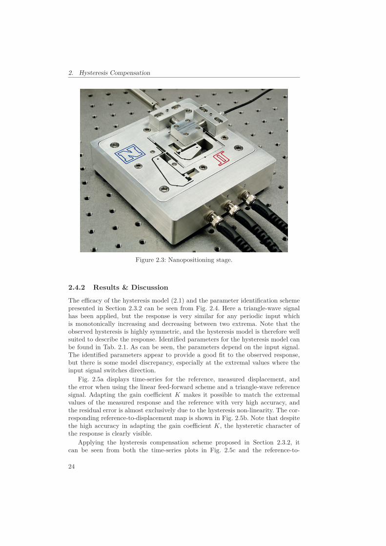
The experimental set-up consisted of a dSPACE DS1103 hardware-in-the-loop sys-tem, an ADE 6810 capacitive gauge and an ADE 6501 capacitive probe from ADETechnologies, a Piezodrive PDL200 voltage amplifier, the custom-made long-rangeserial-kinematic nanopositioner from EasyLab (see Fig. 2.3), two SIM 965 pro-grammable filters and a SIM983 scaling amplifier from Stanford Research Systems.Details on the design of nanopositioner can be found in [120].
The capacitive measurement has a sensitivity of 1/5 V/μm and the voltageamplifier has a gain of 20 V/V. The programmable filters were used as recon-struction and anti-aliasing filters. The scaling amplifier was used to amplify thesignal from the capacitive gauge in order to maximize the resolution of the quan-tized signal. With the DS1103 system, a sampling frequency of 50 kHz was used inall the experiments. For numerical integration, a third-order Runge-Kutta scheme(Bogacki-Shampine) [62] was used.
The first part of the experiments were done using a triangle-wave referencesignal, where 10% of the signal was replaced by a smooth polynomial around theextremal points to reduce vibrations. A second set of experiments was done usinga filtered pseudo random binary signal (PRBS). This signal had a length of 38750samples, a bandwidth of 40 Hz, a ±5 μm range, and was filtered by a second-orderlow-pass Butterworth filter with a 10 Hz cut-off frequency. All the experimentswere performed using feed-forward compensation only.
23
2. Hysteresis Compensation
Figure 2.3: Nanopositioning stage.
2.4.2 Results & Discussion
The efficacy of the hysteresis model (2.1) and the parameter identification schemepresented in Section 2.3.2 can be seen from Fig. 2.4. Here a triangle-wave signalhas been applied, but the response is very similar for any periodic input whichis monotonically increasing and decreasing between two extrema. Note that theobserved hysteresis is highly symmetric, and the hysteresis model is therefore wellsuited to describe the response. Identified parameters for the hysteresis model canbe found in Tab. 2.1. As can be seen, the parameters depend on the input signal.The identified parameters appear to provide a good fit to the observed response,but there is some model discrepancy, especially at the extremal values where theinput signal switches direction.
Fig. 2.5a displays time-series for the reference, measured displacement, andthe error when using the linear feed-forward scheme and a triangle-wave referencesignal. Adapting the gain coefficient K makes it possible to match the extremalvalues of the measured response and the reference with very high accuracy, andthe residual error is almost exclusively due to the hysteresis non-linearity. The cor-responding reference-to-displacement map is shown in Fig. 2.5b. Note that despitethe high accuracy in adapting the gain coefficient K, the hysteretic character ofthe response is clearly visible.
Applying the hysteresis compensation scheme proposed in Section 2.3.2, itcan be seen from both the time-series plots in Fig. 2.5c and the reference-to-
24

2.4. Experimental Results & Discussion
Input Voltage (V)
Dis
plac
emen
t (μm
)
Measured ResponseHysteresis Model Response
Figure 2.4: The input-output map when using a 5 Hz triangle-wave reference signalwith 5 μm amplitude.
displacement map in Fig. 2.5d, that there is a significant reduction in the error.The reduction in maximum error is approximately 90% from when applying a lin-ear feed-forward scheme, to when applying the hysteresis compensation scheme.Most of the residual error when applying the hysteresis compensation scheme isdue to the model discrepancy near the extremal values of the reference signal.
Assessing the performance under non-ideal conditions was done using the fil-tered PRBS reference. The continuous repetition of a PRBS sequence is a periodicsignal, but for the duration of the sequence it behaves as a non-periodic signal, andthe filtered signal is therefore not monotonically varying between only two extrema.The results for the linear feed-forward scheme are shown in Fig. 2.6a, and the re-sults when using the hysteresis compensation scheme are found in Fig. 2.6b. Theerror obtained when using the hysteresis compensation scheme is still significantlylower than when using the linear feed-forward scheme, producing a reduction inmaximum error of approximately 59%. It is apparent, however, that the effective-ness is reduced compared to when applying the triangle-wave signal.
The maximum errors observed for some different configurations of the referencesignal are presented in Tab. 2.2. The reduction in error is found as 100×(1−eh/el)where eh and el are the maximal errors, max(|r − w|), when using the hysteresiscompensation scheme, and linear feed-forward, respectively.
If the parameters of the hysteresis model are fixed, applying the compensation
25
2. Hysteresis Compensation
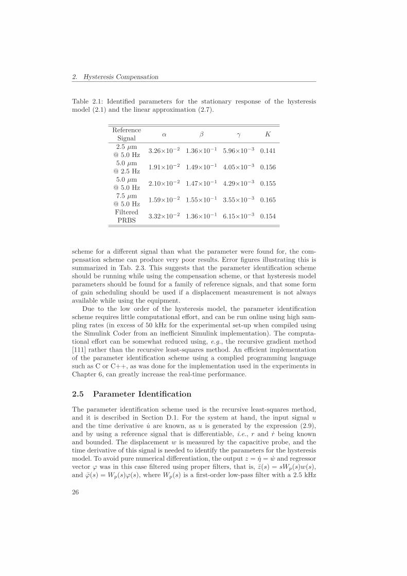
Table 2.1: Identified parameters for the stationary response of the hysteresismodel (2.1) and the linear approximation (2.7).
Referenceα β γ KSignal
2.5 μm 3.26×10⁻² 1.36×10⁻¹ 5.96×10⁻³ 0.141@ 5.0 Hz5.0 μm 1.91×10⁻² 1.49×10⁻¹ 4.05×10⁻³ 0.156@ 2.5 Hz5.0 μm 2.10×10⁻² 1.47×10⁻¹ 4.29×10⁻³ 0.155@ 5.0 Hz7.5 μm 1.59×10⁻² 1.55×10⁻¹ 3.55×10⁻³ 0.165@ 5.0 HzFiltered 3.32×10⁻² 1.36×10⁻¹ 6.15×10⁻³ 0.154PRBS
scheme for a different signal than what the parameter were found for, the com-pensation scheme can produce very poor results. Error figures illustrating this issummarized in Tab. 2.3. This suggests that the parameter identification schemeshould be running while using the compensation scheme, or that hysteresis modelparameters should be found for a family of reference signals, and that some formof gain scheduling should be used if a displacement measurement is not alwaysavailable while using the equipment.
Due to the low order of the hysteresis model, the parameter identificationscheme requires little computational effort, and can be run online using high sam-pling rates (in excess of 50 kHz for the experimental set-up when compiled usingthe Simulink Coder from an inefficient Simulink implementation). The computa-tional effort can be somewhat reduced using, e.g., the recursive gradient method[111] rather than the recursive least-squares method. An efficient implementationof the parameter identification scheme using a complied programming languagesuch as C or C++, as was done for the implementation used in the experiments inChapter 6, can greatly increase the real-time performance.
2.5 Parameter Identification
The parameter identification scheme used is the recursive least-squares method,and it is described in Section D.1. For the system at hand, the input signal uand the time derivative u are known, as u is generated by the expression (2.9),and by using a reference signal that is differentiable, i.e., r and r being knownand bounded. The displacement w is measured by the capacitive probe, and thetime derivative of this signal is needed to identify the parameters for the hysteresismodel. To avoid pure numerical differentiation, the output z = η = w and regressorvector ϕ was in this case filtered using proper filters, that is, z(s) = sWp(s)w(s),and ϕ(s) = Wp(s)ϕ(s), where Wp(s) is a first-order low-pass filter with a 2.5 kHz
26

2.5. Parameter Identification
0 0.05 0.1 0.15 0.2 0.25 0.3 0.35 0.4
0
1
2
3
4
5
Time (s)
Dis
plac
emen
t (m
)
0 0.05 0.1 0.15 0.2 0.25 0.3 0.35 0.4
0
0.1
0.2
0.3
0.4
0.5
Erro
r (m
)
ReferenceMeasurementError
(a) Time-series for the reference signal, andthe stationary measured displacement and er-ror when using linear feed-forward.
0 0.05 0.1 0.15 0.2 0.25 0.3 0.35 0.4
0
1
2
3
4
5
Time (s)
Dis
plac
emen
t (m
)
0 0.05 0.1 0.15 0.2 0.25 0.3 0.35 0.4
0
0.1
0.2
0.3
0.4
0.5
Erro
r (m
)
ReferenceMeasurementError
(b) Time-series for the reference signal, andthe stationary measured displacement and er-ror when using hysteresis compensation.
0
0
Reference (μm)
Mea
sure
d D
ispl
acem
ent (μm
)
(c) Reference-to-displacement map when usinglinear feed-forward.
0
0
Reference (μm)
Mea
sure
d D
ispl
acem
ent (μm
)
(d) Reference-to-displacement map when usinghysteresis compensation.
Figure 2.5: Triangle-wave reference at 5 Hz with 5.0 μm amplitude (4.5 μm linearrange), cf. Tabs. 2.1 and 2.2.
0 0.1 0.2 0.3 0.4 0.5 0.6 0.7
0
1
2
3
4
5
Time (s)
Dis
plac
emen
t (m
)
0 0.1 0.2 0.3 0.4 0.5 0.6 0.7
0
0.2
0.4
0.6
1
Erro
r (m
)
ReferenceMeasurementError
(a) Time-series for the reference signal, andthe stationary measured displacement and er-ror when using linear feed-forward.
0 0.1 0.2 0.3 0.4 0.5 0.6 0.7
0
1
2
3
4
5
Time (s)
Dis
plac
emen
t (m
)
0 0.1 0.2 0.3 0.4 0.5 0.6 0.7
0
0.2
0.4
0.6
1
Erro
r (m
)
ReferenceMeasurementError
(b) Time-series for the reference signal, andthe stationary measured displacement and er-ror when using hysteresis compensation.
Figure 2.6: Filtered PRBS reference, cf. Tabs. 2.1 and 2.2.
27

2. Hysteresis Compensation
Table 2.2: Maximum stationary error when using linear feed-forward and the hys-teresis compensation scheme.
Linear HysteresisFeed-Forward Compensation
Reference Absolute Relative Absolute Relative ErrorSignal Error Error Error Error Reduction2.5 μm 0.20 μm 8.3% 0.016 μm 0.67% 92%@ 5.0 Hz5.0 μm 0.54 μm 11% 0.055 μm 1.1% 90%@ 2.5 Hz5.0 μm 0.54 μm 11% 0.045 μm 0.92% 92%@ 5.0 Hz7.5 μm 0.93 μm 13% 0.053 μm 0.72% 94%@ 5.0 HzFiltered 0.71 μm 13% 0.30 μm 5.4% 59%PRBS
Table 2.3: Maximum stationary error when using the hysteresis compensationscheme with parameter values found for a reference signal other than the oneapplied.
Reference Absolute RelativeSignal Error Error2.5 μm 0.28 μm 12% using parameters found for@ 5.0 Hz 7.5 μm amplitude reference7.5 μm 0.67 μm 9.2% using parameters found for@ 5.0 Hz 2.5 μm amplitude reference
cut-off frequency. Pure numerical differentiation is not desired as it will amplifymeasurement noise, degrading the performance of the identification scheme. If themeasured signal w contains a bias component, filtering z and ϕ by identical high-pass filters with a cut-off frequency lower than the lowest frequency component inthe input signal u can be used to improve estimates.
2.6 Derivation of the Equivalent Coleman-Hodgdon Model
Eq. (2.1) can be solved explicitly, by observing that is can be written as
η = (β − αη + γu) (u)+ + (β + αη − γu) (u)−
where (u)+ = u and (u)− = 0 when u ≥ 0, and (u)+ = 0 and (u)− = u whenu < 0. The dependence on time can then be cancelled. What is left are two linear
28
2.6. Derivation of the Equivalent Coleman-Hodgdon Model
differential equations for the two cases. For the case u ≥ 0 the solution of
dη = (β − αη + γu) du ⇒ dη
du+ αη = β + γu
can be found as
η = e−h
∫eh (β + γu) du = e−αu
[(αβ − γ + αγu)eαu
α2 + C1
],
where eh, h =∫
α du = αu has been used as the integrating factor. This yields
η+ =γ
αu +
αβ − γ
α2 + C1e−αu , (2.18)
where
η0 =γ
αu0 +
αβ − γ
α2 + C1e−αu0 ⇒ C1 = eαu0
(η0 − αβ − γ
α2 − γ
αu0
).
Similarly, for the case u < 0 the solution is
η− =γ
αu +
γ − αβ
α2 + C2eαu , (2.19)
whereC2 = e−αu0
(η0 − γ − αβ
α2 − γ
αu0
).
The solutions (2.18) and (2.19), can be put on the form
η =γ
αu + ηh, (2.20)
which is the form in (2.2), where ηh accounts for the hysteretic behavior. As ithappens, ηh can be taken to be the solution of the differential equation in (2.3),which is
ηh = −bu − aηh|u| . (2.21)
The parameters of this formulation are related to the parameters in (2.1) by
a = α > 0 , b =γ − αβ
α> 0 , and c =
γ
α> 0 . (2.22)
Eq. (2.3) is similar to a case of the well known Dahl solid friction model [53], exceptfor the sign of the parameter b. This equation can also be solved for the cases u ≥ 0and u < 0 in a similar fashion as above, using, e.g., separation of variables. Thesolution for u ≥ 0 is
η+h =
1a
(−b − C3e−au)=
αβ − γ
α2 − 1α
C3e−αu , (2.23)
where
C3 = eau0 (−b − aηh0) = −αeαu0
(η0 − αβ − γ
α2 − γ
αu0
)= −αC1 ,
29

2. Hysteresis Compensation
and for u < 0 it isη−
h =1a(b − C4eau) , (2.24)
whereC4 = e−au0 (b − aηh0) = −αC2 .
By substitution of (2.23) and (2.24) into (2.20) and using the relations in (2.22), itcan be seen that the two formulations are equivalent, by comparison to (2.18) and(2.19).
It can be noted that the solution of (2.21), ηh, is bounded. As
limu→+∞ η+
h (u) = − b
a(2.25)
andlim
u→−∞ η−h (u) =
b
a(2.26)
it is apparent that ‖ηh‖∞ = ba .
2.7 Derivation of the Hysteresis Compensation Scheme
As was shown in Section 2.3.2, by applying the input (2.11), i.e.,
uh =K
cu − 1
cηh , (2.27)
using an estimate of ηh, the effect of the hysteresis can be cancelled.An open-loop observer to estimate ηh can be obtained from (2.3), substituting
uh for the input u, which results in (2.12), that is,
˙ηh = −buh − aηh |uh| = −b
(K
cu − 1
c˙ηh
)− aηh
∣∣∣∣Kc u − 1c˙ηh
∣∣∣∣ .
This expression can be rewritten as
˙ηh =
{K −aηh−b
−aηh−b+c u , uh ≥ 0K aηh−b
aηh−b+c u , uh < 0, (2.28)
but the switching criterion can not be determined causally, as it is dependent onuh and not u.
The expression (2.28) can again be solved explicitly by separation of variablesby canceling the dependence on time. For the case uh ≥ 0,
dη+h
du= K
−aη+h − b
−aη+h − b + c
,
which solution is found as
η+h − c
aln (aη+
h + b) = Ku + C5 ,
30

2.8. Passivity of the Hysteresis Model
whereC5 = ηh0 − c
aln (aηh0 + b) − Ku0 .
This implicit equation can be solved explicitly for ηh as a function of u by usingthe Lambert W function [47], denoted LW (·):
η+h = − c
aLW
(−1
cexp
(−aKu + aC5 + b
c
))− b
a(2.29)
Similarly, for the case uh < 0,
η−h +
c
aln (−aη−
h + b) = Ku + C6 ,
whereC6 = ηh0 +
c
aln (−aηh0 + b) − Ku0 ,
and the explicit solution is found as
η−h =
c
aLW
(−1
cexp
(aKu + aC6 − b
c
))+
b
a. (2.30)
Now, differentiating (2.29) or (2.30) by u yields
dηh
du< 0
in either case. Thus, sincedηh
du=
˙ηh
u, (2.31)
u ≥ 0 ⇒ ˙ηh ≤ 0, and u ≤ 0 ⇒ ˙ηh ≥ 0. Therefore uh ≥ 0 ⇒ u ≥ 0 anduh < 0 ⇒ u < 0. This shows that (2.28) is equivalent to (2.13).
The solution of (2.13), ηh, is also bounded, by similar argument as in Section2.6, and since LW (0) = 0. Thus ‖ηh‖∞ = b
a .
2.8 Passivity of the Hysteresis Model
If a storage function is chosen as
V =12
(cu2 +
1b
ηh2)+ uηh,
the total derivative of V along the trajectories of (2.2) and (2.3) is
V = cuu +1b
ηh (−bu − aηh|u|) + uηh + uηh =
(cu + ηh)u − a
bηh
2|u| = ηu − a
bηh
2|u| ≤ ηu ,
thus, the model (2.2) and (2.3) is passive from u to η.
31
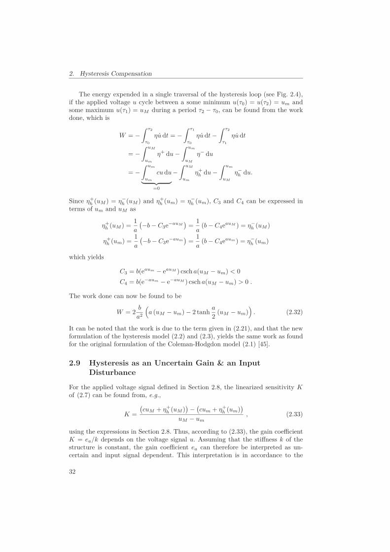
2. Hysteresis Compensation
The energy expended in a single traversal of the hysteresis loop (see Fig. 2.4),if the applied voltage u cycle between a some minimum u(τ0) = u(τ2) = um andsome maximum u(τ1) = uM during a period τ2 − τ0, can be found from the workdone, which is
W = −∫ τ2
τ0
ηu dt = −∫ τ1
τ0
ηu dt −∫ τ2
τ1
ηu dt
= −∫ uM
um
η+ du −∫ um
uM
η− du
= −∫ um
um
cu du︸ ︷︷ ︸=0
−∫ uM
um
η+h du −
∫ um
uM
η−h du.
Since η+h (uM ) = η−
h (uM ) and η+h (um) = η−
h (um), C3 and C4 can be expressed interms of um and uM as
η+h (uM ) =
1a
(−b − C3e−auM)=
1a(b − C4eauM ) = η−
h (uM )
η+h (um) =
1a
(−b − C3e−aum)=
1a(b − C4eaum) = η−
h (um)
which yields
C3 = b(eaum − eauM ) csch a(uM − um) < 0C4 = b(e−aum − e−auM ) csch a(uM − um) > 0 .
The work done can now be found to be
W = 2b
a2
(a (uM − um) − 2 tanh
a
2(uM − um)
). (2.32)
It can be noted that the work is due to the term given in (2.21), and that the newformulation of the hysteresis model (2.2) and (2.3), yields the same work as foundfor the original formulation of the Coleman-Hodgdon model (2.1) [45].
2.9 Hysteresis as an Uncertain Gain & an InputDisturbance
For the applied voltage signal defined in Section 2.8, the linearized sensitivity Kof (2.7) can be found from, e.g.,
K =(cuM + η+
h (uM ))− (
cum + η+h (um)
)uM − um
, (2.33)
using the expressions in Section 2.8. Thus, according to (2.33), the gain coefficientK = ea/k depends on the voltage signal u. Assuming that the stiffness k of thestructure is constant, the gain coefficient ea can therefore be interpreted as un-certain and input signal dependent. This interpretation is in accordance to the
32
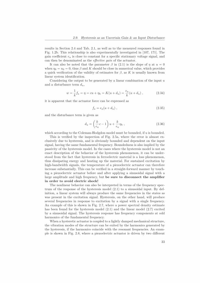
2.9. Hysteresis as an Uncertain Gain & an Input Disturbance
results in Section 2.4 and Tab. 2.1, as well as to the measured responses found inFig. 1.2b. This relationship is also experimentally investigated in [107, 171]. Thegain coefficient ea is close to constant for a specific stationary voltage signal, andcan then be denominated as the effective gain of the actuator.
It can also be noted that the parameter β in (2.1) is the slope of η at u = 0when η0 = u0 = 0, thus β and K should be close in numerical value, which providesa quick verification of the validity of estimates for β, as K is usually known fromlinear system identification.
Considering the output to be generated by a linear combination of the input uand a disturbance term du,
w =1k
fa = η = cu + ηh = K(u + du) =ea
k(u + du) , (2.34)
it is apparent that the actuator force can be expressed as
fa = ea(u + du) , (2.35)
and the disturbance term is given as
du =(
k
eac − 1
)u +
k
eaηh , (2.36)
which according to the Coleman-Hodgdon model must be bounded, if u is bounded.This is verified by the inspection of Fig. 2.5a, where the error is almost ex-
clusively due to hysteresis, and is obviously bounded and dependent on the inputsignal, having the same fundamental frequency. Boundedness is also implied by thepassivity of the hysteresis model. In the cases where the hysteresis model is not anexact description of the behavior of the hysteresis phenomenon, it can be under-stood from the fact that hysteresis in ferroelectric material is a loss phenomenon,thus dissipating energy and heating up the material. For sustained excitation byhigh-bandwidth signals, the temperature of a piezoelectric actuator can thereforeincrease substantially. This can be verified in a straight-forward manner by touch-ing a piezoelectric actuator before and after applying a sinusoidal signal with alarge amplitude and high frequency, but be sure to disconnect the amplifierin order to avoid electric shock!
The nonlinear behavior can also be interpreted in terms of the frequency spec-trum of the response of the hysteresis model (2.1) to a sinusoidal input. By def-inition, a linear system will always produce the same frequencies in the states aswas present in the excitation signal. Hysteresis, on the other hand, will produceseveral frequencies in response to excitation by a signal with a single frequency.An example of this is shown in Fig. 2.7, where a power spectral density estimatehas been found for the hysteresis model (2.1) and the linear model (2.7) excitedby a sinusoidal signal. The hysteresis response has frequency components at oddharmonics of the fundamental frequency.
When a hysteretic actuator is coupled to a lightly damped mechanical structure,the vibration modes of the structure can be exited by the harmonics generated bythe hysteresis, if the harmonics coincide with the resonant frequencies. An exam-ple is shown in Fig. 2.8, where a piezoelectric actuator is driven by two different
33

2. Hysteresis Compensation
0 5 10 15 20 25 30 35 40 45 50
0
20
40
Frequency (Hz)
Pow
er/fr
eque
ncy
(dB
/Hz)
Hysteresis ResponseLinear Response
Figure 2.7: Power spectral density estimate for the hysteresis model and the linearmodel, when excited using a 1 Hz sinusoid.
0 0.001 0.002 0.003 0.004 0.005 0.006 0.007 0.008 0.009 0.01
0
1
2
3
Time (s)
Dis
plac
emen
t (μm
)
Measured ResponseIdeal Linear Response
(a) Measured response using a 30 V amplitudesinusoid at 150.0 Hz.
0 0.001 0.002 0.003 0.004 0.005 0.006 0.007 0.008 0.009 0.01
0
1
2
3
Time (s)
Dis
plac
emen
t (μm
)
Measured ResponseIdeal Linear Response
(b) Measured response using a 30 V amplitudesinusoid at 178.3 Hz.
Figure 2.8: Excitation of vibration dynamics with a resonant frequency of 535 Hzby actuator hysteresis.
sinusoidal voltage signals and the coupled mechanical structure has a dominantvibration mode with a resonant frequency at 535 Hz. If the input signal has afrequency of 150.0 Hz, there does not seem to be any significant excitation of anyvibration modes, but if the frequency is increased to 178.3 Hz, which has a firstodd harmonic of 534.9 Hz, the dominant vibration mode is excited.
34
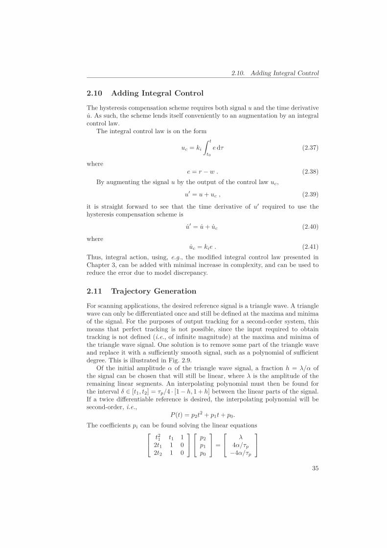
2.10. Adding Integral Control
2.10 Adding Integral Control
The hysteresis compensation scheme requires both signal u and the time derivativeu. As such, the scheme lends itself conveniently to an augmentation by an integralcontrol law.
The integral control law is on the form
uc = ki
∫ t
t0
edτ (2.37)
wheree = r − w . (2.38)
By augmenting the signal u by the output of the control law uc,
u′ = u + uc , (2.39)
it is straight forward to see that the time derivative of u′ required to use thehysteresis compensation scheme is
u′ = u + uc (2.40)
whereuc = kie . (2.41)
Thus, integral action, using, e.g., the modified integral control law presented inChapter 3, can be added with minimal increase in complexity, and can be used toreduce the error due to model discrepancy.
2.11 Trajectory Generation
For scanning applications, the desired reference signal is a triangle wave. A trianglewave can only be differentiated once and still be defined at the maxima and minimaof the signal. For the purposes of output tracking for a second-order system, thismeans that perfect tracking is not possible, since the input required to obtaintracking is not defined (i.e., of infinite magnitude) at the maxima and minima ofthe triangle wave signal. One solution is to remove some part of the triangle waveand replace it with a sufficiently smooth signal, such as a polynomial of sufficientdegree. This is illustrated in Fig. 2.9.
Of the initial amplitude α of the triangle wave signal, a fraction h = λ/α ofthe signal can be chosen that will still be linear, where λ is the amplitude of theremaining linear segments. An interpolating polynomial must then be found forthe interval δ ∈ [t1, t2] = τp/4 · [1− h, 1+ h] between the linear parts of the signal.If a twice differentiable reference is desired, the interpolating polynomial will besecond-order, i.e.,
P (t) = p2t2 + p1t + p0.
The coefficients pi can be found solving the linear equations⎡⎣ t2
1 t1 12t1 1 02t2 1 0
⎤⎦⎡⎣ p2
p1p0
⎤⎦ =
⎡⎣ λ
4α/τp
−4α/τp
⎤⎦
35

2. Hysteresis Compensation
t
r(t)
{p /20
Figure 2.9: Modified triangle wave.
where t1 = τp/4 · (1 − h) and t2 = τp/4 · (1 + h). Similarly, if a higher number ofderivatives is desired, higher order polynomials should be used. With this method,to ensure that only the highest order derivative necessary will be discontinuous,the polynomial must be of order np = 2nd − 2, where nd is the number of desiredderivatives.
The first half of the reference signal can now be computed as
r(t) =
⎧⎨⎩
4ατp
t , t ∈ [0, t1)p2t2 + p1t + p0 , t ∈ [t1, t2]
− 4ατp
t , t ∈ (t2, τp/2),
r(t) =
⎧⎨⎩
4ατp
, t ∈ [0, t1)2p2t + p1 , t ∈ [t1, t2]
− 4ατp
, t ∈ (t2, τp/2),
and
r(t) =
⎧⎨⎩
0 , t ∈ [0, t1)2p2 , t ∈ [t1, t2]0 , t ∈ (t2, τp/2)
.
The last half can be generated by inverting the first half and shifting it by τp/2.
2.12 Conclusions
In this Chapter a feed-forward hysteresis compensation scheme was proposed forpiezoelectric actuators. The scheme is based on a reformulation of the Coleman-Hodgdon model, where the reformulation produces a mathematically equivalentinput-output map. The original Coleman-Hodgdon model can be used for parame-ter identification, while the reformulation can be used to generate an estimate thehysteretic response and to linearize the input-output map.
Since the parameters used in the scheme are identified online, the method willprovide consistent performance, even when the hysteretic response changes due todifferent reference signals and other factors such as depolarization of the materialand actuator temperature.
36

2.12. Conclusions
The proposed method is well suited for the case of symmetric hysteretic re-sponses and certain periodic reference trajectories. The method has low complexityand is thus readily applicable for real-time implementation.
Experimental results are presented to illustrate the hysteresis compensationscheme. The experiments showed that the method reduced the hysteretic behaviorof a piezoelectric actuator significantly, providing a reduction of more than 90%compared to when when assuming a linear response.
In addition, the reformulation of the Coleman-Hodgdon model has a form thatmakes it straight forward to show passivity of the model. The reformulation, sinceit is equivalent, has the same energy dissipation for a primitive hysteresis loop asthe original formulation. The response of the model can also be interpreted as anuncertain gain and an input disturbance, and the hysteresis compensation schemecan be augmented with a integral control law in a straight forward manner, whichcan improve tracking performance.
37


Part II
Damping & Tracking Control
39


Chapter 3
Damping & Tracking ControlSchemes for Nanopositioning
3.1 Introduction
Tracking control for nanopositioning devices can be achieved using feed-forwardand feedback control techniques. Although feed-forward techniques can providevery good results [44], feedback control may be necessary in order to reduce sen-sitivity to uncertainty and disturbances. In order to control lightly damped vibra-tional modes in active structures, several control schemes that introduce damp-ing have been developed. These include fixed-structure, low-order control laws,such as positive position feedback [76], integral force feedback [174], passive shunt-damping [96], resonant control [170], and integral resonant control [13]. By couplingsuch schemes with an integral control law, significantly better reference trackingperformance can be achieved. With the exception of passive shunt-damping, thishas been experimentally demonstrated in [14, 78, 85]. The main reason for theincreased performance, is that a reduction of the dominant resonant peak in thefrequency response of the system leads to an increased gain margin, enabling muchhigher gain to be used for the reference tracking integral control law [78].
General model-based control laws can also be used, such as H∞-synthesis [206],the linear-quadratic-gaussian regulator [94], or output feedback control laws foundusing pole-placement and model reference control [94, 111]. There are several ex-amples of control laws derived using H∞-synthesis applied to nanopositioning sys-tems [138, 187, 188, 192, 192, 194, 196, 198, 201, 211].
The advantage of using fixed-structure, low-order control laws is mostly prac-tical, as such control laws are simple to implement and have low computationalcomplexity [9]. The simplicity also makes them feasible for implementation usinganalog circuit elements. This can be beneficial, as avoiding sampling and quantiza-tion reduces the noise floor [175, 220]. The disadvantage of using fixed-structure,low-order control laws, is a lack of methods for optimal tuning, and this is along standing and challenging control engineering problem. Although there existsome results for fixed-order control problems solved using linear matrix inequal-ities [56, 73, 95, 104, 109, 113, 210], these methods do not allow for the use of
41
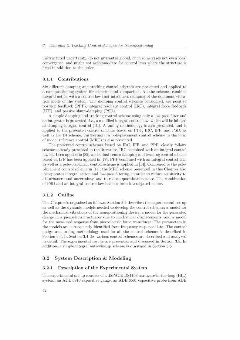
3. Damping & Tracking Control Schemes for Nanopositioning
unstructured uncertainty, do not guarantee global, or in some cases not even localconvergence, and might not accommodate for control laws where the structure isfixed in addition to the order.
3.1.1 Contributions
Six different damping and tracking control schemes are presented and applied toa nanopositioning system for experimental comparison. All the schemes combineintegral action with a control law that introduces damping of the dominant vibra-tion mode of the system. The damping control schemes considered, are positiveposition feedback (PPF), integral resonant control (IRC), integral force feedback(IFF), and passive shunt-damping (PSD).
A simple damping and tracking control scheme using only a low-pass filter andan integrator is presented, i.e., a modified integral control law, which will be labeledas damping integral control (DI). A tuning methodology is also presented, and isapplied to the presented control schemes based on PPF, IRC, IFF, and PSD, aswell as the DI scheme. Furthermore, a pole-placement control scheme in the formof model reference control (MRC) is also presented.
The presented control schemes based on IRC, IFF, and PPF, closely followsschemes already presented in the literature. IRC combined with an integral controllaw has been applied in [85], and a dual-sensor damping and tracking control schemebased on IFF has been applied in [78]. PPF combined with an integral control law,as well as a pole-placement control scheme is applied in [14]. Compared to the pole-placement control scheme in [14], the MRC scheme presented in this Chapter alsoincorporates integral action and low-pass filtering, in order to reduce sensitivity todisturbances and uncertainty, and to reduce quantization noise. The combinationof PSD and an integral control law has not been investigated before.
3.1.2 Outline
The Chapter is organized as follows. Section 3.2 describes the experimental set-upas well as the dynamic models needed to develop the control schemes; a model forthe mechanical vibrations of the nanopositioning device, a model for the generatedcharge in a piezoelectric actuator due to mechanical displacements, and a modelfor the measured response from piezoelectric force transducer. The parameters inthe models are subsequently identified from frequency response data. The controldesign and tuning methodology used for all the control schemes is described inSection 3.3. In Section 3.4 the various control schemes are described and analyzedin detail. The experimental results are presented and discussed in Section 3.5. Inaddition, a simple integral anti-windup scheme is discussed in Section 3.6.
3.2 System Description & Modeling
3.2.1 Description of the Experimental System
The experimental set-up consists of a dSPACE DS1103 hardware-in-the-loop (HIL)system, an ADE 6810 capacitive gauge, an ADE 6501 capacitive probe from ADE
42

3.2. System Description & Modeling
Figure 3.1: Custom flexure-guided nanopositioning stage.
Flexures
Positionsensor
ActuatorMovingplatform
Fixed base
w Forcesensor
Figure 3.2: Simplified schematic of the single degree-of-freedom flexure guided po-sitioning stage.
43
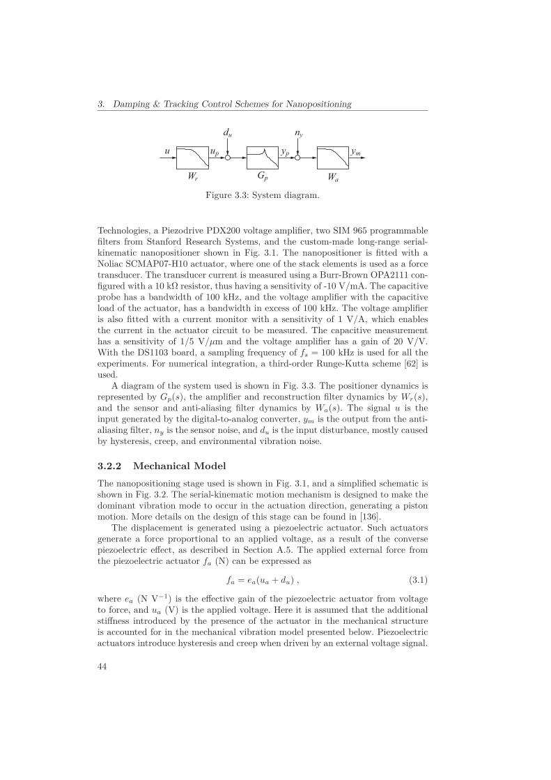
3. Damping & Tracking Control Schemes for Nanopositioning
Wr WaGp
u ymup yp
du ny
Figure 3.3: System diagram.
Technologies, a Piezodrive PDX200 voltage amplifier, two SIM 965 programmablefilters from Stanford Research Systems, and the custom-made long-range serial-kinematic nanopositioner shown in Fig. 3.1. The nanopositioner is fitted with aNoliac SCMAP07-H10 actuator, where one of the stack elements is used as a forcetransducer. The transducer current is measured using a Burr-Brown OPA2111 con-figured with a 10 kΩ resistor, thus having a sensitivity of -10 V/mA. The capacitiveprobe has a bandwidth of 100 kHz, and the voltage amplifier with the capacitiveload of the actuator, has a bandwidth in excess of 100 kHz. The voltage amplifieris also fitted with a current monitor with a sensitivity of 1 V/A, which enablesthe current in the actuator circuit to be measured. The capacitive measurementhas a sensitivity of 1/5 V/μm and the voltage amplifier has a gain of 20 V/V.With the DS1103 board, a sampling frequency of fs = 100 kHz is used for all theexperiments. For numerical integration, a third-order Runge-Kutta scheme [62] isused.
A diagram of the system used is shown in Fig. 3.3. The positioner dynamics isrepresented by Gp(s), the amplifier and reconstruction filter dynamics by Wr(s),and the sensor and anti-aliasing filter dynamics by Wa(s). The signal u is theinput generated by the digital-to-analog converter, ym is the output from the anti-aliasing filter, ny is the sensor noise, and du is the input disturbance, mostly causedby hysteresis, creep, and environmental vibration noise.
3.2.2 Mechanical Model
The nanopositioning stage used is shown in Fig. 3.1, and a simplified schematic isshown in Fig. 3.2. The serial-kinematic motion mechanism is designed to make thedominant vibration mode to occur in the actuation direction, generating a pistonmotion. More details on the design of this stage can be found in [136].
The displacement is generated using a piezoelectric actuator. Such actuatorsgenerate a force proportional to an applied voltage, as a result of the conversepiezoelectric effect, as described in Section A.5. The applied external force fromthe piezoelectric actuator fa (N) can be expressed as
fa = ea(ua + du) , (3.1)
where ea (N V−1) is the effective gain of the piezoelectric actuator from voltageto force, and ua (V) is the applied voltage. Here it is assumed that the additionalstiffness introduced by the presence of the actuator in the mechanical structureis accounted for in the mechanical vibration model presented below. Piezoelectricactuators introduce hysteresis and creep when driven by an external voltage signal.
44

3.2. System Description & Modeling
These effects occur in the electrical domain [161], and it is a reasonable assumptionto consider this behavior as a bounded disturbance added to the input, representedby the term du (V), as discussed in Section 2.9.
As demonstrated in Appendix B, the dynamics due to the applied force fa ofa point w (m) on the flexible structure, as observed by a co-located sensor in anon-gyroscopic reference frame, is adequately described by the following lumpedparameter, truncated linear model
Gw(s) = eaw
fa(s) ≈
nw∑i=1
βi
s2 + 2ζiωis + ωi2 + Dr , (3.2)
where nw is the number of vibration modes included. Here, {βi} (m s−2 V−1)are the control gains, {ζi} are the damping coefficients for each mode, and {ωi}(rad s−1) are the natural frequencies for the modes. The term Dr (m V−1) is theresidual mode, which is an approximation of the non-modeled higher frequencymodes, and can be included to improve prediction of zero-locations. It produces amodel that is not strictly proper, but as the instrumentation, such as the amplifierand sensors, have limited bandwidth, Dr can be considered equal to zero for thissystem. Eq. (3.2) has a pole-zero interleaving property [172], which is the originof positive-realness (passivity) and negative-imaginariness for certain input-outputpairs [166]. The inclusion of instrumentation dynamics, and sensor-actuator pairsthat are not perfectly co-located, will in general invalidate the pole-zero interleavingproperty [172].
3.2.3 Charge
When applying passive shunt-damping, the generated charge due to the directpiezoelectric effect in the actuator circuit is utilized. This is sometimes referred toas self-sensing. As is shown in Section A.4, or equivalently from the constitutiveequations in stress-charge from Section A.5, the induced charge in the actuator is
q = eaw + Cpua = Cp(ua + αw) ,
where Cp (F) is the capacitance of the piezoelectric stack actuator, and α = ea/Cp
(V m−1) is a constant determining the amount of charge generated by the directpiezoelectric effect due to the displacement w of the mechanical structure. Thetransfer-function from applied voltage ua to induced charge q is therefore
Gq(s) =q
ua(s) = Cp(1 + αGw(s)) . (3.3)
3.2.4 Force Transducer
The integral force feedback scheme utilizes a co-located sensor in the form of apiezoelectric force transducer. The force sensor generates a charge, depending onthe applied force, due to the direct piezoelectric effect.
From Section A.5 it is known that the constitutive equations in strain-chargeform provides an expression for the charge in a piezoelectric transducer as
q = dafa + Cp(1 + k2)ua .
45

3. Damping & Tracking Control Schemes for Nanopositioning
For sensing, there is no applied voltage, thus ua = 0, and the charge on the elec-trodes of the sensor can be found to be
q = dafa .
Since the force working on the sensor is the same as the force working on theactuator, the force must be according to the constitutive equations in stress-chargeform,
fa = kaw − eaua ,
and the induced charge in the sensor can be found to be
q = da(kaw − eaua) .
The current or charge produced by the force transducer is typically convertedto a voltage signal using a simple op-amp circuit with a high input impedance andgain gs (V/C). The output voltage from such a sensor when measuring the charge,can be found to be [78, 172]
vf = ks(w − kf ua) ,
where w is the displacement of the mechanical structure, ua is the applied voltageto the actuator, kf = ea/ka (m V−1) is the gain of the feed-through term, andks = gsdaka (V m−1) is the sensor gain. The transfer-function from applied voltageua to measured sensor voltage vf can therefore be found as
Gf (s) =vf
ua(s) = ks(Gw(s) − kf ) . (3.4)
3.2.5 Identification & Uncertainty
In order to identify the parameters in (3.2), (3.3), and (3.4), the frequency responsesfor the displacement, charge, and force are recorded using a SR780 Dynamic SignalAnalyzer from Stanford Research Systems, applying a 150 mV RMS bandwidth-limited white noise excitation signal. The models are fitted into the procured datausing the MATLAB System Identification and Optimization Toolboxes. As thenoise from the force transducer is orders of magnitude lower than the noise fromthe displacement sensor [78], the frequency response for the displacement is inferredfrom (3.4). The frequency response obtained using the displacement sensor is usedto find the parameters in (3.3) and (3.4). The responses for Gw(s), Gq(s), and Gf (s)are displayed in Figs. 3.4a, 3.5a, and 3.6a, respectively. The identified parametervalues are presented in Tab. 3.1. For the displacement model (3.2), three vibrationmodes, nd = 3, are included. By inspection of Fig. 3.4a, it can be seen that thesecond mode at 1660 Hz is the dominant piston mode.
The uncertainty of the models can be quantified as unstructured multiplica-tive perturbations. Since the control schemes considered are either single-input-single-output (SISO), or single-input-multiple-output (SIMO), the uncertainty de-scription of the models from the scalar input up to the output vector yp has theform [100]
ypi = Gi(s)(1 + δi(s)Δi(s))up ; ‖Δi(s)‖∞ ≤ 1 , (3.5)
46

3.3. Control Design
Table 3.1: Identified model parameters.
Parameter Value UnitDisplacement model (3.2)
β1 1.80·104 μm s−2 V−1
ζ1 0.0726ω1 2π·490 rad s−1
β2 2.54·106 μm s−2 V−1
ζ2 0.0196ω2 2π·1660 rad s−1
β3 4.83·106 μm s−2 V−1
ζ3 0.0312ω3 2π·3400 rad s−1
Charge model (3.3)Cp 195 nFα 3.95 V μm−1
Force model (3.4)ks 2.52·10−7 V μm−1
kf 0.0451 μm V−1
where i denotes the index into the output vector yp, such that Gi(s) correspondsto the transfer-function from the input up to the output ypi, and δi(s) is thecorresponding frequency dependent uncertainty weight. The uncertainty weights{δi(s)} are determined experimentally, for each of the outputs, and are presented inFigs. 3.4b, 3.5b, and 3.6b. Over-bounding weights were also found to introduce moreconservativeness. The gain uncertainty discussed in Section 2.9 is here downplayedsomewhat as the maximum range of the nanopositioning device will not be usedin the experiments and to simplify the choice of uncertainty weights, as they areactually coupled.
3.3 Control Design
The control schemes presented will be analyzed with regards to the general controlstructure shown in Fig. 3.7.
3.3.1 Performance Measures
The control schemes considered are either single-input-single-output (SISO), orsingle-input-multiple-output (SIMO). Considering the general SIMO case, it can
47

3. Damping & Tracking Control Schemes for Nanopositioning
Mag
nitu
de (d
B)
Phas
e (d
eg)
Frequency (Hz)
Measured responseModel response
(a) Frequency response for the displacement model Gw(s).
102 103 104
0
20
40
Mag
nitu
de (d
B)
Frequency (Hz)
(b) Multiplicative uncertainty weight δw(s).
Figure 3.4: Response and uncertainty for the displacement.
48

3.3. Control Design
Mag
nitu
de (d
B)
Phas
e (d
eg)
Frequency (Hz)
Measured responseModel response
(a) Frequency response for the charge model Gq(s).
102 103 104
Mag
nitu
de (d
B)
Frequency (Hz)
(b) Multiplicative uncertainty weight δq(s).
Figure 3.5: Response and uncertainty for the charge.
49

3. Damping & Tracking Control Schemes for NanopositioningM
agni
tude
(dB
)Ph
ase
(deg
)
Frequency (Hz)
Measured responseModel response
(a) Frequency response for the force model Gf (s).
102 103 104
0
Mag
nitu
de (d
B)
Frequency (Hz)
(b) Multiplicative uncertainty weight δf (s).
Figure 3.6: Response and uncertainty for the force.
50
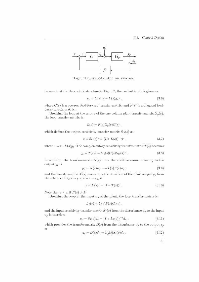
3.3. Control Design
up GpypC
F
r-e
du
ny
Figure 3.7: General control law structure.
be seen that for the control structure in Fig. 3.7, the control input is given as
up = C(s)(r − F (s)yp) , (3.6)
where C(s) is a one-row feed-forward transfer-matrix, and F (s) is a diagonal feed-back transfer-matrix.
Breaking the loop at the error e of the one-column plant transfer-matrix Gp(s),the loop transfer-matrix is
L(s) = F (s)Gp(s)C(s) ,
which defines the output sensitivity transfer-matrix SO(s) as
e = SO(s)r = (I + L(s))−1r , (3.7)
where e = r−F (s)yp. The complementary sensitivity transfer-matrix T (s) becomes
yp = T (s)r = Gp(s)C(s)SO(s)r . (3.8)
In addition, the transfer-matrix N(s) from the additive sensor noise ny to theoutput yp is
yp = N(s)ny = −T (s)F (s)ny , (3.9)
and the transfer-matrix E(s), measuring the deviation of the plant output yp fromthe reference trajectory r, ε = r − yp, is
ε = E(s)r = (I − T (s))r . (3.10)
Note that ε �= e, if F (s) �= I.Breaking the loop at the input up of the plant, the loop transfer-matrix is
LI(s) = C(s)F (s)Gp(s) ,
and the input sensitivity transfer-matrix SI(s) from the disturbance du to the inputup is therefore
up = SI(s)du = (I + LI(s))−1du , (3.11)
which provides the transfer-matrix D(s) from the disturbance du to the output yp
asyp = D(s)du = Gp(s)SI(s)du . (3.12)
51
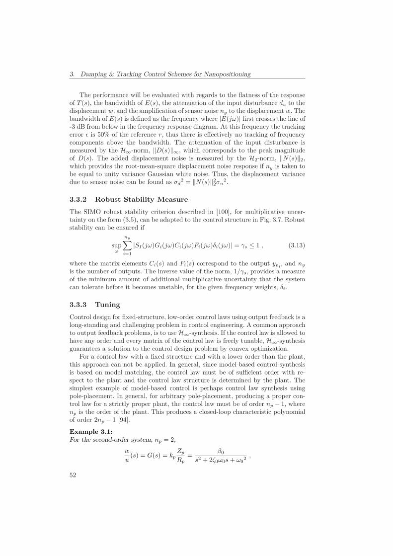
3. Damping & Tracking Control Schemes for Nanopositioning
The performance will be evaluated with regards to the flatness of the responseof T (s), the bandwidth of E(s), the attenuation of the input disturbance du to thedisplacement w, and the amplification of sensor noise ny to the displacement w. Thebandwidth of E(s) is defined as the frequency where |E(jω)| first crosses the line of-3 dB from below in the frequency response diagram. At this frequency the trackingerror ε is 50% of the reference r, thus there is effectively no tracking of frequencycomponents above the bandwidth. The attenuation of the input disturbance ismeasured by the H∞-norm, ‖D(s)‖∞, which corresponds to the peak magnitudeof D(s). The added displacement noise is measured by the H2-norm, ‖N(s)‖2,which provides the root-mean-square displacement noise response if ny is taken tobe equal to unity variance Gaussian white noise. Thus, the displacement variancedue to sensor noise can be found as σd
2 = ‖N(s)‖22σn
2.
3.3.2 Robust Stability Measure
The SIMO robust stability criterion described in [100], for multiplicative uncer-tainty on the form (3.5), can be adapted to the control structure in Fig. 3.7. Robuststability can be ensured if
supω
ny∑i=1
|SI(jω)Gi(jω)Ci(jω)Fi(jω)δi(jω)| = γs ≤ 1 , (3.13)
where the matrix elements Ci(s) and Fi(s) correspond to the output ypi, and ny
is the number of outputs. The inverse value of the norm, 1/γs, provides a measureof the minimum amount of additional multiplicative uncertainty that the systemcan tolerate before it becomes unstable, for the given frequency weights, δi.
3.3.3 Tuning
Control design for fixed-structure, low-order control laws using output feedback is along-standing and challenging problem in control engineering. A common approachto output feedback problems, is to use H∞-synthesis. If the control law is allowed tohave any order and every matrix of the control law is freely tunable, H∞-synthesisguarantees a solution to the control design problem by convex optimization.
For a control law with a fixed structure and with a lower order than the plant,this approach can not be applied. In general, since model-based control synthesisis based on model matching, the control law must be of sufficient order with re-spect to the plant and the control law structure is determined by the plant. Thesimplest example of model-based control is perhaps control law synthesis usingpole-placement. In general, for arbitrary pole-placement, producing a proper con-trol law for a strictly proper plant, the control law must be of order np − 1, wherenp is the order of the plant. This produces a closed-loop characteristic polynomialof order 2np − 1 [94].
Example 3.1:For the second-order system, np = 2,
w
u(s) = G(s) = kp
Zp
Rp=
β0
s2 + 2ζ0ω0s + ω02 ,
52

3.3. Control Design
a first-order proper control law of
C(s) =B(s)A(s)
=b1s + b0
s + a0,
can be found for arbitrary pole-placement conforming to the third-order polynomial
P (s) = s3 + p2s2 + p1s1 + p0 ,
by solving the Bézout identity
Rp(s)A(s) + kpZp(s)B(s) = P (s) .
The solution for the control law parameters θc = [a0, b1, b0]T is
Sθc = p =
⎡⎣ 1 0 02ζ0ω0 β0 0ω0
2 0 β0
⎤⎦⎡⎣a0
b1b0
⎤⎦ =
⎡⎣p2 − 2ζ0ω0
p1 − ω02
p0
⎤⎦ ⇒ θc = S−1p .
Here, three freely tunable control law parameters are needed in order to specifythe poles. If the plant model is of higher order, the control law order grows, andin general, for a control law of minimal order, no constraints on the control lawstructure can be made. Second-order pole-placement is also possible for the second-order system using a proportional-derivative (PD) control law, but in this case thecontrol law is not proper, and might cause implementation problems in terms ofnoise amplification and insufficient roll-off for the loop transfer-function G(s)C(s)at higher frequencies, due to the derivative action.
For standard mixed H∞-synthesis, the minimum control law order is also de-termined by the plant order, but the performance and robust stability weights willtypically add to the complexity of the control law. Moreover, the exact choice ofweighs directly impacts the closed-loop performance. If the resulting control lawis of very high order, practical problems related to numerical stability, discretiza-tion, and computational complexity can arise. Due to the limited computationalpower available when using high sampling frequencies, or if an implementation us-ing analog circuit elements is desired, the model order should be as low a possible.Applying model or control law order reduction techniques can provide some rem-edy, but can in some cases lead to unexpected results, and will in any case add acomplicating step in the control design.
There exist some results for direct synthesis of low-order robust control prob-lems, solved with the use of linear matrix inequalities. However, these methods donot allow for the use of unstructured uncertainty, do not guarantee global, and inmany cases not even local, convergence, and might not accommodate for controllaws where the structure is fixed in addition to the order [56, 73, 95, 104, 109, 113,210].
In other words, there does not exist any general control design method for out-put feedback using fixed-structure, low-order control laws. A practical optimizationprocedure is therefore proposed in order to obtain good tracking performance.
53

3. Damping & Tracking Control Schemes for Nanopositioning
Tuning Methodology
Control design is often a trade-off between conflicting goals. For nanopositioningsystems, it is desirable to have a high bandwidth for E(s) in order to have goodreference tracking. Also, the system is required to well damped in order to avoidexcessive vibrations. This translates to an absence of peaks in T (s). To counter hys-teresis and creep, as well as environmental disturbances, D(s) must provide a highdegree of attenuation. In addition, the amplification of sensor noise should be assmall as possible, meaning that N(s) should have the smallest bandwidth possible.Due to the restriction imposed by the Bode sensitivity integral [94], it is impossi-ble to meet these criteria simultaneously. As the purpose of damping control is toreduce peaks in the closed-loop response due to lightly damped vibration modes,and since ideal tracking performance is achieved when T (s) = 1, it appears that agood overall performance criterion is the flatness of T (s), i.e., the minimization of
J(θc) = ‖1 − |T (jω, θc)|‖2 , (3.14)
by some optimal control law parameter vector θc�.
For the control schemes presented in the following sections, with the exceptionof model reference control, a practical and straight forward method to find controllaw parameters θc that provide good tracking performance for a particular schemeis to solve
arg minθc
J(θc) s.t. Re{λi} ∈ R− ∧ γs < 1 , (3.15)
where {λi} is the set of eigenvalues for the closed-loop system.The optimization problem can be solved either by using an exhaustive grid
search over a domain of reasonable control law parameter values, as is demonstratedfor the DI scheme in Chapter 4, or by using an unstructured optimization algorithm,such as the Nelder-Mead method [133]. In this Chapter, all the control schemes weretuned using the Nelder-Mead method.
3.4 Damping & Tracking Control Schemes
3.4.1 Integral Control Law
An integral control law applied to a mass-spring-damper system has a fairly limitedgain margin. When applied to a lightly damped structure, the integral gain isprimarily limited by the resonant frequency and relative damping of the dominantvibration mode.
Considering an integral control law
Ci(s) =ki
s
where ki > 0, applied to a mass-spring-damper system
w
u(s) =
β0
s2 + 2ζ0ω0s + ω02 ,
54

3.4. Damping & Tracking Control Schemes
Ct Cd Wr Gw Waua w
–r
–u
du nw
Figure 3.8: Control structure when using positive position feedback and integralresonant control.
where β0 > 0, an analytical expression for the maximum gain k∗i that renders
a stable closed-loop system can be found by application of the Routh-Hurwitzcriterion, as
ki <2ζ0ω0
3
β0= k∗
i . (3.16)
Given a lightly damped system, 0 < ζ0 1/√2, knowing the resonant frequency
ωp and the amplitude response at resonance |G(jωp)|, cf. Section B.3,
ωp = ω0
√1 − 2ζ0
2 and |G(jωp)| = β0
2ζ0ω02√1 − ζ0
2,
the maximum gain (3.16) can be expressed as
ki <ωp
|G(jωp)| < κ1 · ωp
|G(jωp)| = k∗i (3.17)
where κ1−1 =
√1 − ζ0
2 ·√1 − 2ζ0
2 < 1. This corresponds well with the resultfound in [78], where (3.17) is derived by graphical arguments. The example above isfor a single degree of freedom system, but the analysis corresponds well to multipledegree of freedom systems where there is one dominant vibration mode and norigid body modes.
It is clear that the integral gain is limited by both the natural frequency ofthe dominant vibration mode, and the amount of damping in the structure. Itcan be therefore be conjectured that attenuating the resonant peak or increasingthe resonant frequency improves the gain margin, and thus the bandwidth of theclosed-loop system.
3.4.2 Positive Position Feedback (PPF)
Damping and tracking control using positive position feedback (PPF) [76, 172]combined with an integral control law can be implemented using the control struc-ture in Fig. 3.8. This is equivalent to the control scheme in [14]. The dampingcontrol law consists of a low-pass filter with negative gain
Cd(s) =−kd
s2 + 2ζdωds + ωd2 , (3.18)
were kd > 0 is the control law gain, ζd the damping coefficient and ωd is the cut-offfrequency. The tracking control law, is an integral control law with a negative gain,
55

3. Damping & Tracking Control Schemes for Nanopositioning
which will be inverted by the negative gain of the filter (3.18),
Ct(s) =−kt
s. (3.19)
Here, kt > 0 is the gain of the integral term.To analyze the nominal performance of the control scheme, the control struc-
ture in Fig. 3.8 can be put on the equivalent formulation adhering to the controlstructure in Fig. 3.7. The feed-forward filter is found as
C(s) = Wr(s)Cd(s)Ct(s) , (3.20)
and the feedback filter is found as
F (s) = Wa(s)(1 + C−1t (s)) . (3.21)
Using the above expressions, and assuming
Gp(s) = Gw(s) ,
it is straight forward to find the transfer-functions for the sensitivity (3.7), thecomplementary sensitivity (3.8), the noise attenuation (3.9), the error attenuation(3.10), and the disturbance rejection (3.12). Here, Wr(s) = Wa(s), and are second-order Butterworth filters with cut-off frequency at 20 kHz.
The robust stability with regards to the multiplicative model uncertainty canbe evaluated using the stability criterion (3.13), using (3.8), (3.20) and (3.21).
There are four tunable control law parameters
θc = [kd, ζd, ωd, kt]T ,
the feedback filter gain kd, the damping ratio ζd, the cut-off frequency ωd, andthe tracking integral control law gain kt. The optimal control law parameters for(3.18) and (3.19) found when solving (3.15) are presented in Tab. 3.2. The resultingnominal frequency responses for T (S), E(s), and D(s) are shown in Fig. 3.16a.
Table 3.2: Optimal parameters for (3.18) and (3.19).
Parameter Valuekd 2.32·108
ζd 0.564ωd 2π·1470kt 2.31·104
Additional Analysis
Stability of the PPF scheme is straight forward to analyze considering the negative-imaginary property of the low-pass filter (3.18) and the mechanical vibration model(3.2) [166].
56

3.4. Damping & Tracking Control Schemes
Inverting the gain of the low-pass filter (3.18), i.e.,
C(s) =kd
s2 + 2ζdωds + ωd2 , (3.22)
it is known that this is a strictly negative-imaginary (SNI) transfer-function [166].The mechanical vibration model (3.2) is also SNI, as it is a linear combination ofSNI transfer-functions, where each transfer-function has the same form as (3.22),and since the real constant term Dr does not influence the negative imaginary prop-erties. Negative imaginariness can also be established by the pole-zero interleavingproperty described in Appendix B, as ∠Gw(jω) ∈ [−180◦, 0◦].
Since both transfer-functions are SNI, the positive feedback connection of C(s)and Gw(s) is therefore internally stable if C(0)Gw(0) < 1.
However, the closed-loop transfer-function
Tppf (s) =−C(s)Gw(s)1 − C(s)Gw(s)
=Cd(s)Gw(s)
1 + Cd(s)Gw(s),
is not negative-imaginary (NI), and further analysis using negative-imaginary prop-erties can not be done. Also, including instrumentation dynamics and not havingperfect co-location of the sensor and actuator precludes the usage of NI analysis. Itshould be noted, however, that with reasonably good co-location for the dominantvibration modes, and instrumentation with significantly higher bandwidth thanthe dominant vibration modes, modeling the control law and plant dynamics using(3.18) and (3.2) provides a good approximation and good results in practice.
3.4.3 Integral Resonant Control (IRC)
Damping and tracking control applying integral resonant control (IRC) [13] tointroduce damping can also be implemented using the control structure in Fig. 3.8.In this control scheme [85] the damping control law is
Cd(s) =−kd
s + kdDf. (3.23)
Eq. (3.23) is the result of rearranging the IRC scheme to a form suitable for trackingcontrol [85], consistent with the control structure in Fig. 3.8. Here, kd > 0 is thecalled the integral damping gain, while Df > 0 is a feedthrough term. The trackingcontrol law is
Ct(s) =−kt
s, (3.24)
where kt > 0 is the gain of the integral term.As this scheme uses the same control structure as the one using PPF in Sec-
tion 3.4.2, the scheme can be analyzed using the same equivalent formulation withregards to the general control structure in Fig. 3.7, i.e., with
C(s) = Wr(s)Cd(s)Ct(s) (3.25)
andF (s) = Wa(s)(1 + C−1
t (s)) . (3.26)
57
3. Damping & Tracking Control Schemes for Nanopositioning
uawr
+ vf
hp
lpnw
nf
–r
Gw
Gf
Ci
a
a
u
du
Figure 3.9: Control structure when using integral force feedback.
Here, Wr(s) = Wa(s), and are second-order Butterworth filters with cut-off fre-quency at 20 kHz.
There are three tunable control parameters
θc = [Df , kd, kt]T ,
the feedthrough term Df , the integral damping gain kd, and the tracking integralcontrol law gain kt. The optimal control law parameters for (3.23) and (3.24) foundwhen solving (3.15) are presented in Tab. 3.3. The resulting nominal frequencyresponses for T (S), E(s), and D(s) are shown in Fig. 3.16b.
Table 3.3: Optimal parameters for (3.23) and (3.24).
Parameter ValueDf 0.116kd 8.75·104
kt 7.12·103
Remark 3.1. Inverting the gain of the transfer-function (3.23), i.e.,
C(s) =kd
s + kdDf,
it is known that it is a strictly negative-imaginary transfer-function [27, 166]. Theexact same arguments can then be made for internal stability as in the PPF case,assuming perfect co-location and no instrumentation dynamics.
3.4.4 Integral Force Feedback (IFF)
The dual-sensor damping and tracking control scheme proposed in [78], is based onintegral force feedback (IFF) [172, 174], and can be implemented using the controlstructure shown in Fig. 3.9, where Gf (s) is described in (3.4).
The advantage of using this scheme, is that the piezoelectric force transducerhas a noise density orders of magnitude lower than a capacitive probe, thus allowing
58
3.4. Damping & Tracking Control Schemes
high bandwidth, but with substantially lower displacement noise due to feedback.The drawback is reduced range, as the force sensor replaces parts of the actuator,and additional instrumentation to amplify the charge generated by the transducer.The force sensor also requires good calibration, and the response is slightly non-linear, but this is an insignificant source of error at higher frequencies.
The control scheme requires an integral control law,
Ci(s) =ki
s, (3.27)
to be implemented, where ki > 0 is the gain. In addition, two splitting filters, alow-pass and a high-pass filter, must be implemented. The low-pass filter is givenas
Wlp(s) =ωf
s + ωf, (3.28)
while the high-pass filter is given as
λWhp(s) = λs
s + ωf, (3.29)
where the gain λ is found as
λ =∣∣∣∣Gw(0)Gf (0)
∣∣∣∣ . (3.30)
The cut-off frequency ωf determines split between the frequency range for whereto use displacement feedback, and where to use force feedback. For the implemen-tation, this was chosen to be ωf = 2π · 50. Better noise properties can be achievedby reducing ωf , but this is limited to some extent by the need to high-pass filterthe force measurement. The high-pass filter is used both to allow the use of thecapacitive probe measurement at low frequencies, and to remove bias componentsin the charge measurement. As the force transducer response is slightly non-linear,sufficient bandwidth for the capacitive probe measurement is required to improvelinearity.
This is a single-input-multiple-output (SIMO) system, and the measurementvector is given as
yp = [w, vf ]T , (3.31)
while the input is the applied voltage ua. With regards to Fig. 3.7, the planttransfer-matrix is
Gp(s) = [Gw(s), Gf (s)]T , (3.32)
the feed-forward transfer-matrix is given as
C(s) = [Wr(s)Ci(s), −Wr(s)Ci(s)] , (3.33)
and the feedback transfer-matrix is given as
F (s) =[WlpWa(s) 0
0 λWhpWa
]. (3.34)
Here, Wr(s) = Wa(s), and are second-order Butterworth filters with cut-off fre-quency at 20 kHz.
59

3. Damping & Tracking Control Schemes for Nanopositioning
There is one tunable control parameter
θc = ki ,
the integral gain ki. The optimal control law parameter for (3.27) found whensolving (3.15) is presented in Tab. 3.4. It can also be found using a root-locus plot,or an approximate analytical expression [78, 172]. The resulting nominal frequencyresponses for T (s), E(s), and D(s) are shown in Fig. 3.16c.
Table 3.4: Optimal parameter for (3.27).
Parameter Valueki 1.37·105
Additional Analysis
Neglecting the instrumentation dynamics and assuming perfect co-location, stabil-ity of the IFF scheme can be analyzed using the negative-imaginary property of(3.4) and the product of (3.27) and (3.29), i.e.,
C(s) = λWhp(s)Ci(s) =λki
s + ωf. (3.35)
By the definition of a strictly negative-imaginary (SNI) transfer-function [166],the transfer-function (3.4) is SNI since all the poles of Gf (s) are in the open lefthalf of the complex plane, and since
j [Gf (jω) − Gf (−jω)] = ks
nw∑i=1
4βiζiωiω
(ωi2 − ω2)2 + (2ζiωiω)2
> 0 ∀ ω > 0 .
Similarly, for (3.35), the pole of C(s) is in the open left half of the complex plane,and
j[C(jω) − C(−jω)
]=
2λkiω
ωf2 + ω2 > 0 ∀ ω > 0 ,
thus (3.35) is also SNI. The positive feedback connection of Gf (s) and C(s) istherefore internally stable, if C(0)Gf (0) < 1.
Closing the loop for the force feedback path in Fig. 3.9 yields
Gw(s) =w
ua(s) =
Gw
1 − λWhp(s)Ci(s)Gf (s)
for the response from applied voltage ua to the displacement w, which is stable bythe above arguments. This is not a negative-imaginary (NI) transfer-function, andfurther analysis using NI properties can not be done.
60

3.4. Damping & Tracking Control Schemes
us
q
+ uq=
Cp+
R L
Z(s) ua
Figure 3.10: Actuator circuit with shunt.
uawrq
nw
– Wr
Gw
Gq
Ci
Wa
sZ
–u us
du
Figure 3.11: Control structure when using passive shunt-damping.
Now, closing the loop for the displacement feedback path in Fig. 3.9 yields
T11(s) =w
r(s) =
Ci(s)Gw(s)1 + Wlp(s)Ci(s)Gw(s)
=
Ci(s)Gw(s)1 + Ci(s)(Wlp(s)Gw(s) − λWhp(s)Gf (s))
,
and for a model Gw(s) with more than one vibration mode, or if instrumentationdynamics is included, no algebraic roots can be found. However, using a sufficientlylow cut-off frequency ωf , the complementary sensitivity function from r to w can,since Wlp(s) + Whp(s) = 1, be approximated as
T11(s) =Ci(s)Gw(s)
1 − λCi(s)Gf (s) + Wlp(s)Ci(s) (Gw(s) + λGf (s))≈ Ci(s)Gw(s)
1 − λCi(s)Gf (s),
which is an unconditionally stable transfer-function [81]. It corresponds to the casewhen only applying IFF without the high-pass filter [172], and feed-forward filteringthe reference through the integral control law. The approximation is also valid forinstrumentation dynamics with sufficiently high bandwidth.
3.4.5 Passive Shunt-Damping (PSD)
Passive shunt-damping [96] can introduce damping by adding an inductor and aresistor in series with the piezoelectric actuator, which acts as a capacitor, due
61

3. Damping & Tracking Control Schemes for Nanopositioning
to the large dielectric constant of the piezoelectric material. Tuning the resultingLCR-circuit for maximal damping creates a resonant LCR-circuit that works anal-ogously to a tuned mechanical absorber. This is physically realized as shown in Fig.3.10. Adding an integral control law for tracking, results in the control structureshown in Fig. 3.11, where Gq(s) is as given in (3.3). As discussed below, this config-uration does not result in the same tuning of the LCR-circuit when optimizing fora flat frequency magnitude response for the complementary sensitivity function,compared to the case when optimizing for maximum damping (in the absence ofthe integral control law).
The transfer-function for the added shunt in Fig. 3.10 is
Z(s) = sL + R , (3.36)
where L (H) is the inductance, and R (Ω) is the resistance. The integral controllaw is
Ci(s) =ki
s, (3.37)
where ki > 0 is the gain.This can be interpreted as a single-input-multiple-output (SIMO) system, where
the measurement vector is given as
y = [d, vf ]T , (3.38)
and the input is the applied voltage ua. With regards to Fig. 3.7, the plant transfer-matrix is
Gp(s) = [Gw(s), Gq(s)]T , (3.39)
the feed-forward transfer-matrix is
C(s) = [Wr(s)Ci(s), sZ(s)] , (3.40)
and the feedback transfer-matrix is given by
F (s) =[Wa(s) 00 1
]. (3.41)
Here, Wr(s) = Wa(s), and are second-order Butterworth filters with cut-off fre-quency at 20 kHz.
There are three tunable control parameters
θc = [L, R, ki]T ,
the shunt inductance L, the shunt resistance R, as well as the tracking integralcontrol law gain ki. The optimal control law parameters for (3.36) and (3.37) foundwhen solving (3.15) are presented in Tab. 3.5. The resulting nominal frequencyresponses for T (S), E(s), and D(s) are shown in Fig. 3.16d.
The shunt was implemented using an inductor constructed using a closed ferritecore and approximately 45 turns of copper wire. A potentiometer was used toimplement the required resistance. The inductor and resistor were tuned to theirrequired values using an Agilent U1733C LCR meter.
62
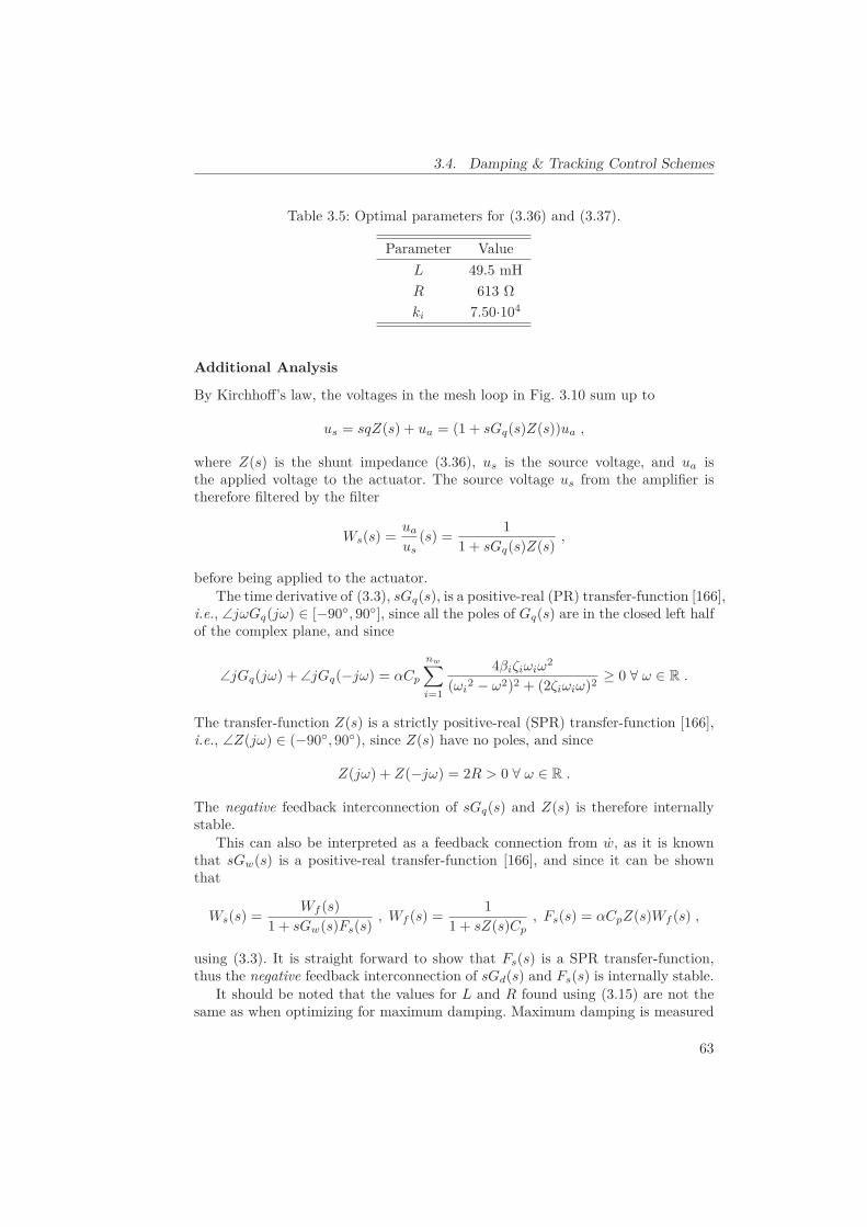
3.4. Damping & Tracking Control Schemes
Table 3.5: Optimal parameters for (3.36) and (3.37).
Parameter ValueL 49.5 mHR 613 Ωki 7.50·104
Additional Analysis
By Kirchhoff’s law, the voltages in the mesh loop in Fig. 3.10 sum up to
us = sqZ(s) + ua = (1 + sGq(s)Z(s))ua ,
where Z(s) is the shunt impedance (3.36), us is the source voltage, and ua isthe applied voltage to the actuator. The source voltage us from the amplifier istherefore filtered by the filter
Ws(s) =ua
us(s) =
11 + sGq(s)Z(s)
,
before being applied to the actuator.The time derivative of (3.3), sGq(s), is a positive-real (PR) transfer-function [166],
i.e., ∠jωGq(jω) ∈ [−90◦, 90◦], since all the poles of Gq(s) are in the closed left halfof the complex plane, and since
∠jGq(jω) + ∠jGq(−jω) = αCp
nw∑i=1
4βiζiωiω2
(ωi2 − ω2)2 + (2ζiωiω)2
≥ 0 ∀ ω ∈ R .
The transfer-function Z(s) is a strictly positive-real (SPR) transfer-function [166],i.e., ∠Z(jω) ∈ (−90◦, 90◦), since Z(s) have no poles, and since
Z(jω) + Z(−jω) = 2R > 0 ∀ ω ∈ R .
The negative feedback interconnection of sGq(s) and Z(s) is therefore internallystable.
This can also be interpreted as a feedback connection from w, as it is knownthat sGw(s) is a positive-real transfer-function [166], and since it can be shownthat
Ws(s) =Wf (s)
1 + sGw(s)Fs(s), Wf (s) =
11 + sZ(s)Cp
, Fs(s) = αCpZ(s)Wf (s) ,
using (3.3). It is straight forward to show that Fs(s) is a SPR transfer-function,thus the negative feedback interconnection of sGd(s) and Fs(s) is internally stable.
It should be noted that the values for L and R found using (3.15) are not thesame as when optimizing for maximum damping. Maximum damping is measured
63

3. Damping & Tracking Control Schemes for Nanopositioning
with regards to the increase in disturbance rejection when adding the shunt to thepiezoelectric actuator, i.e.,
D(s) =w
du(s) =
Gw(s)1 + sGw(s)Fs(s)
.
For applications when reduced sensitivity to environmental disturbances is desired,and there is no need for reference tracking or if reference tracking is preformed byfeed-forward control, this can be achieved solving, e.g.,
arg minR,L
∥∥D(jω, R, L)∥∥
2 . (3.42)
For the system at hand, this results in L = 46.6 mH and R = 165 Ω, whichproduces a resonant LCR-circuit response, due to the much smaller resistancevalue. An approximate value for the inductance can also be found assuming theshunt-circuit forms an harmonic oscillator with an undamped natural frequencyequal to the undamped natural frequency of the vibration mode that should bedamped. Then the inductance will be
L ≈ 1Cpω22 = 47.1mH . (3.43)
The resonant response can be seen in Fig. 3.12a, which displays the response ofWf (s), which accounts for the LCR-circuit alone.
An example of the decreased input disturbance sensitivity due to the presence ofa shunt tuned for maximum damping is shown in Fig. 3.13. Here, experimental timeresponses to the signal us = Wf (s)−1r, r being a triangle-wave signal, are shown.It is immediately apparent that the excitation of a vibration mode is significantlyreduced due to the shunt.
The response obtained for Wf (s) when using the values of L and R from Tab. 3.5is almost identical to that of a second-order low-pass Butterworth filter with cut-offfrequency ωc =
√1/LCp.
From Fig. 3.12b, which displays the response of Ws(s), where also the generatedcharge is taken into account, it can be seen that for the values from Tab. 3.5,the response is still very similar to the Butterworth filter, although there is someadditional damping introduced due to the uq = αGw(s) term in (3.3).
Since
Gw(s) =w
us(s) =
Gw(s)1 + sZ(s)Gq(s)
= Ws(s)Gw(s) =
Wf (s)Gw(s)1 + sGw(s)Fs(s)
= Wf (s)D(s)
when the shunt is present, the source voltage us is filtered by Ws(s) before it isapplied to the actuator, or equivalently, the source voltage us can be seen as a inputdisturbance filtered by Wf (s), where Fs(s) can be interpreted to be a feedback filter.Responses for D(s) and Gw(s) are shown in Figs. 3.12c and 3.12d, respectively, fordifferent parameter values for L and R. Although the parameter values obtained
64

3.4. Damping & Tracking Control Schemes
Mag
nitu
de (d
B)
Phas
e (d
eg)
Frequency (Hz)
Butterworth filterWf (sWf (s
(a) LCR filter, Wf (s), compared to a Butter-worth filter.
Mag
nitu
de (d
B)
Phas
e (d
eg)
Frequency (Hz)
Butterworth filterW
s(s
Ws(s
(b) Source voltage filter, Ws(s), compared to aButterworth filter.
Mag
nitu
de (d
B)
Phas
e (d
eg)
Frequency (Hz)
Gw
(s)
D(sD(s
(c) Disturbance attenuation, D(s), compared tothe system without the shunt, Gw(s).
Mag
nitu
de (d
B)
3
Phas
e (d
eg)
Frequency (Hz)
Gw
(s)
w(s
w(s
(d) Response from source voltage to displace-ment, Gw(s), compared to the system withoutthe shunt, Gw(s).
Figure 3.12: Results when considering passive shunt-damping alone, using differentoptimality criteria.
when solving (3.42) provides greater damping of the dominant vibration mode, theparameter values obtained when solving (3.15) produces the flattest response forT11(s) when also including feedback using the integral control law (3.37).
For tracking control, using the optimality criterion (3.14), this means that theshunt can be approximated by a low-pass Butterworth filter, which is done inSection 3.4.6, where the anti-aliasing and reconstruction filters are used to introducedamping.
It might also be noted that when using passive shunt-damping, the low-passfilter Ws(s) makes the use of the anti-aliasing filter Wa(s) unnecessary. However,a potential practical problem when implementing the shunt using passive compo-nents, is to find a high-quality inductor with a sufficiently high inductance value,especially when the dominant resonant frequency is fairly low, due to (3.43).
65

3. Damping & Tracking Control Schemes for Nanopositioning
0 0.005 0.01 0.015 0.02 0.025 0.03 0.035 0.04
0
0.1
0.2
0.3
0.4
0.5
Time (s)
Dis
plac
emen
t (μm
)
Input ± 20 volt @ 48 Hz
Without shuntWith shunt
(a) Response to filtered triangle wave with fun-damental frequency at 48 Hz.
0 0.001 0.002 0.003 0.004 0.005 0.006 0.007 0.008 0.009 0.01
0
0.1
0.2
0.3
0.4
0.5
Time (s)
Dis
plac
emen
t (μm
)
Input ± 20 volt @ 138 Hz
Without shuntWith shunt
(b) Response to filtered triangle wave with fun-damental frequency at 138 Hz.
Figure 3.13: Time-series of the response when applying feed-forward control whenshunt circuit is present, using us = Wf (s)−1r.
3.4.6 Damping Integral Control (DI)
As noted in Section 3.4.5, the optimal values for the resistance and inductance forthe shunt, when solving (3.15), result in a low-pass filter when connected to the ca-pacitance of the actuator, with approximately the same response as a second-orderlow-pass Butterworth filter. Implementing a control scheme on a microcontrolleror a computer, there must be anti-aliasing and reconstruction filters present in or-der to avoid aliasing and to reduce quantization noise. Instead of applying a shuntcircuit, the reconstruction and anti-aliasing filters that are already present as partof the instrumentation can be used, as long as the cut-off frequency is below theNyquist frequency. The resulting control structure is shown in Fig. 3.14.
Similarly to the case when using passive shunt-damping, only an integral controllaw needs to be implemented, i.e.,
Ci(s) =ki
s, (3.44)
where ki > 0 is the gain. The cut-off frequency, ωc, for the filters Wr(s) and Wa(s)must be tuned as well. Here it is assumed that Wr(s) = Wa(s) for simplicity. Thefilters used in the experimental set-up are second order Butterworth filters, i.e.,
Wr(s) = Wa(s) =ωc
2
s2 +√2ωcs + ωc
2. (3.45)
The combined filter Wr(s)Wa(s) is of fourth order, but the closed-loop response ofthe system is almost identical to the case when using a passive shunt. The addedbenefit is that the shunt is no longer needed, and that off-the-shelf programmablefilters that are easy to tune can be used.
Formulating the control scheme in terms of the general control structure inFig. 3.7, the feed-forward filter is
C(s) = Wr(s)Ci(s) (3.46)
66

3.4. Damping & Tracking Control Schemes
Ci Wr Gw Waua w
–r u
du nw
Figure 3.14: Control structure when introducing damping by applying a low-passfilter in the signal chain, in this case by utilizing the filter Wr(s)Wa(s).
Table 3.6: Optimal parameters for (3.44) and (3.45).
Parameter Valueωc 2π·2150ki 6.68·104
and the feedback filter isF (s) = Wa(s) . (3.47)
There are two tunable control parameters
θc = [ωc, ki]T ,
the filter cut-off frequency ωc, and the tracking integral control law gain ki. Theoptimal control law parameters for (3.44) and (3.45) found when solving (3.15) arepresented in Tab. 3.6. The resulting nominal frequency responses for T (S), E(s),and D(s) are shown in Fig. 3.16e.
Additional Analysis
The combined control law, consisting of (3.44) and (3.45), has an extra degree offreedom, in the choice of the cut-off frequency ωc of the filters (3.45). In the simplestform, the control law consist of an integrator and a second-order low-pass filter, andis applied to a second-order mass-spring-damper system. The closed-loop system istherefore, at minimum, of fifth order, and has no algebraic roots. The control lawhas two free parameters, ki and ωc. The control law will therefore not lend itself topolynomial coefficient matching. The practical solution is to investigate the effectsof the low-pass filters in the signal chain using numerical analysis.
This is done in Fig. 3.15, where the eigenvalue loci for the closed-loop systemis plotted as a function of the cut-off frequency ωc. Here, Gd(s) together with C(s)and F (s), as defined in (3.46) and (3.47), is used.
The integral control law gain ki is in this example set using (3.17). It is ap-parent that tuning the integral control law to the stability margin k∗
i = 1.75 · 104,the system is either unstable or close to being unstable when using high cut-offfrequencies for the anti-aliasing and reconstruction filters. However, as the rootloci in Fig. 3.15 indicate, reducing the cut-off frequencies for the filters, all eigen-values can be moved further into the left-half plane, and there appears to be anoptimal value for the cut-off frequency. By moving the poles further into the right
67

3. Damping & Tracking Control Schemes for Nanopositioning
Re( )
Im(
)
(a) The positive imaginary part of the com-plex conjugate eigenvalue loci for the vibrationmodes in addition to the modes due to the fil-ters (3.45), and the real valued mode due to theintegral control law (3.44).
Re( )
Im(
)
c
c
(b) The first vibration mode, cf. Tab. 3.1.
Re( )
Im(
)
c
c
(c) The second vibration mode, cf. Tab. 3.1.Re( )
Im(
)
c
c
(d) The third vibration mode, cf. Tab. 3.1.
Figure 3.15: Eigenvalue loci for the closed-loop system as a function of the filtercut-off frequency ωc. The loci are symmetric about the real axis.
half-plane, the gain margin for the closed-loop system will be larger. This shouldallow for a higher closed-loop bandwidth.
It should be noted the reducing the cut-off frequency ωc all the way towardszero, one of the modes close to the origin will move into the right half-plane. Thereis therefore a domain of values of ωc for which the system is stable.
Inspecting Fig. 3.15, one might expect that minimizing the maximum value ofthe real part of the eigenvalues for the closed-loop system as a function of the cut-off frequency ωc will provide the fastest system. For the model Gd(s), this resultsin
arg minωc∈R+/{0}
[arg maxRe(λ)∈R−
[det(A(ωc) − λI) = 0]] = 2π · 1110 rad/s , (3.48)
where A(ωc) is a state matrix realization for the closed-loop system for a givenωc. Solving (3.48) will move all the eigenvalues as far into the left-half plane as
68

3.4. Damping & Tracking Control Schemes
possible, but will not necessarily result in the flattest response when increasingthe integral control gain ki to take advantage of the increased gain margin. Theclosed-loop pole locations are also dependent on the value of ki, thus solving (3.15)seem to be a better approach, as it provides optimal values for both ki and ωc.
According to the results in Section 3.4.5, one might expect the optimal cut-offfrequency ωc to be close to
√1/LCp = 2π · 1620 rad/s, and the integral gain ki
close to be close to the value in Tab. 3.5. Using these values in the filters C(s)and F (s) as defined in (3.46) and (3.47), provides a fairly flat response for thecomplementary sensitivity function, but as would be expected, better results areobtained using the values in Tab. 3.6.
An advantageous side-effect of tuning the anti-aliasing and reconstruction fil-ters to a cut-off frequency close to the bandwidth of the resulting complementarysensitivity function, is an effective attenuation of quantization noise and higher-frequency sensor noise. This provides an improvement in the actual displacementnoise floor of the system. A similar effect is obtained using passive shunt-damping,but in that case only quantization noise is attenuated. For good noise attenuation,it is ideal that the bandwidths of the anti-aliasing and reconstruction filters areas low as possible, and this idea is also applied in the control design of the modelreference control in Section 3.4.7.
For the experimental set-up, the anti-aliasing and reconstruction filters have auser-programmable cut-off frequency ωc. However, most filter topologies are fairlystraight forward to tune, especially the state-variable topology. One-componentfilters with the state-variable topology are readily available from major producersof integrated circuits.
3.4.7 Model Reference Control (MRC)
The model reference control (MRC) [111] objective is to make the plant output yp
track the output of a reference model ym. Similar to polynomial-based control, orpole-placement [94, 111], MRC provides a control law for arbitrary closed-loop poleplacement, but also allows for arbitrary minimum phase zero placement. A second-order pole-placement control law, similar to the control law in Example 3.1, wasapplied to a nanopositioning stage in [15]. The synthesis equations for the MRCscheme are summarized in Appendix E.
For the MRC design, the displacement model of the system Gw(s) is truncatedto only include the dominant piston mode at 1660 Hz, the second mode of thepositioning stage,
Gw(s) =Gd(0)β2/ω22
β2
s2 + 2ζ2ω2s + ω22 . (3.49)
This is done in order to keep the control law order as low as possible, and to avoidexcitation of the vibration modes above the dominant mode. The above model isaugmented with an integrator, in order to reduce the sensitivity to plant uncertaintyat lower frequencies. In addition, the anti-aliasing and reconstruction filters Wr(s)and Wa(s) are incorporated into the control design. The filters provide an additionaldegree of freedom when tuning the control law, and can be used to attenuatenon-modeled high-frequency dynamics, as well as to attenuate quantization and
69

3. Damping & Tracking Control Schemes for Nanopositioning
sensor noise. The complete plant model, with regards to the synthesis equations inAppendix E, is thus taken to be
Gp(s) =1s
Gw(s)Wr(s)Wa(s) , (3.50)
and is of seventh-order. In addition to the plant model Gp(s), there are two addi-tional design choices with regards to the control law; the reference model Wm(s)and the output filter 1/Γ(s). The main limiting factor in determining these filters,is the uncertainty of the plant model, which for the system at hand is mostly dueto non-modeled high-frequency dynamics.
For simplicity, the reference model Wm(s) is chosen to be a seventh-order But-terworth filter with cut-off frequency ωm. Since the plant model Gp(s) does nothave any zeros, Λ(s) should be a polynomial of sixth order. The zeros of Λ(s)were chosen to have a Butterworth pattern with radius ωl. The anti-aliasing andreconstruction filters have a user-programmable cut-off frequency ωc, which can betuned, given that ωc is below the Nyquist frequency.
The design problem is as such reduced to three tunable control parameters
θc = [ωc, ωm, ωl]T ,
the cut-off frequencies ωc, ωm, ωl. The reference model is a Butterworth filter,which is maximally flat by definition. The optimality criterion described in Equa-tion (3.14) is therefore satisfied for all ωm, ωl, and ωc that render a stable closed-loop system. The cut-off frequencies were therefore tuned manually, attempting toobtain the highest bandwidth for E(s) while still having a robustly stable closed-loop system. The control law parameters used are presented in Tab. 3.7.
The implementation of the scheme is done by moving the integrator in (3.50) tothe feed-forward filter, i.e., compared to the scheme as presented in Appendix E,the feed-forward filter (E.7) is augmented as
C(s) =1s
C(s) , (3.51)
but the feedback filter (E.8) is left as it is, i.e.,
F (s) = F (s) . (3.52)
The parameters for the feed-forward filter C(s) and feedback filter F (s) are foundusing (E.5) and (E.6).
With regards to the general control structure in Fig. 3.7, the analysis in termsof the sensitivity (3.7), complementary sensitivity (3.8), noise attenuation (3.9),error attenuation (3.10), and disturbance rejection (3.12) is done using
Gp(s) = Gw(s) , (3.53)
C(s) = C(s)Wr(s) , (3.54)and
F (s) = F (s)Wa(s) . (3.55)The resulting nominal frequency responses for T (S), E(s), and D(s) are shown inFig. 3.16f.
70

3.4. Damping & Tracking Control Schemes
Mag
nitu
de (d
B)
2 3 4
Phas
e (d
eg)
Frequency (Hz)
T(s)E(s)D(s)
(a) Positive position feedback (PPF).M
agni
tude
(dB
)
2 3 4
Phas
e (d
eg)
Frequency (Hz)
T(s)E(s)D(s)
(b) Integral resonant control (IRC).
Mag
nitu
de (d
B)
2 3 4
Phas
e (d
eg)
Frequency (Hz)
T (s)E (s)D (s)
(c) Integral force feedback (IFF).
Mag
nitu
de (d
B)
2 3 4
Phas
e (d
eg)
Frequency (Hz)
T (s)E (s)D (s)
(d) Passive shunt-damping (PSD).
Mag
nitu
de (d
B)
2 3 4
Phas
e (d
eg)
Frequency (Hz)
T(s)E(s)D(s)
(e) Damping integral control (DI).
Mag
nitu
de (d
B)
2 3 4
Phas
e (d
eg)
Frequency (Hz)
T(s)E(s)D(s)
(f) Model reference control (MRC).
Figure 3.16: Nominal frequency responses.
71

3. Damping & Tracking Control Schemes for Nanopositioning
Table 3.7: Control law parameters for MRC.
Parameter Valueωc 2π·3000ωm 2π·2000ωl 2π·2250
3.5 Experimental Results & Discussion
The six different control schemes were implemented on the hardware-in-the-loopsystem, and the tracking performance when using a triangle-wave reference signalwith a fundamental frequency of 80 Hz and an amplitude of 1 μm was recordedfor each scheme. The fundamental frequency of the reference signal was chosen inorder for the 21st harmonic of the signal to be close to the dominant vibrationmode. The displacement for all the schemes was measured on a separate channelusing an anti-aliasing filter with a 35 kHz cut-off frequency. The generated currentfrom the force transducer was measured, and integrated numerically. The cut-offfrequency for the anti-aliasing filter for this measurement was always set to 20 kHz,for all the experiments.
3.5.1 Results
Nominal frequency responses for the various schemes are presented in Figs. 3.16a,3.16b, 3.16c, 3.16d, 3.16e, and 3.16f. The measures from Section 3.3 are summarizedin Tab. 3.8. Note that the values for 1/γs are not directly comparable between SISOand SIMO systems.
The results when tracking a triangle-wave reference signal are presented inFigs. 3.17 and 3.18. The maximum error (ME) ranges from 15% to 24%, and theroot-mean-square error (RMSE) ranges from 0.11 μm to 0.20 μm. The error valuesare also summarized in Tab. 3.8. Note that tracking performance can be increasedby adding feed-forward, but this is not done in order for the error signals to besignificantly larger than the noise in the measured displacement signal, to avoidobfuscating the actual results achieved due to feedback.
3.5.2 Discussion
The best performing control schemes in terms of the error are the scheme usingintegral force feedback (IFF) and the model reference control (MRC) scheme. Theworst performance is obtained when using positive position feedback (PPF) and thedamping integral control (DI) scheme, while when using integral resonant control(IRC) and passive shunt-damping (PSD), errors in the middle of the range areobtained.
The error figures in terms of ME and RMSE can be changed by the control lawtuning, but a reduction in RMSE typically leads to an increase in ME, due to amore oscillatory response.
72

3.5. Experimental Results & Discussion
Table 3.8: Bandwidth of E(s), ||N(s)||2 from nw to w, ||D(s)||∞ from du to w,1/γs, root-mean-square error (RMSE), and maximum error (ME) obtained for thecontrol schemes.
Scheme BW ||N(s)||2 ||D(s)||∞ 1/γs RMSE ME
PPF 318 Hz 61.1 191×10−3 1.66 0.194 μm 0.231 μm
IRC 369 Hz 78.4 281×10−3 1.01 0.173 μm 0.213 μm
IFF 329 Hz 12.6 424×10−4 1.14 0.123 μm 0.146 μm
PSD 338 Hz 60.0 139×10−3 1.14 0.178 μm 0.218 μm
DI 372 Hz 58.6 204×10−3 1.66 0.197 μm 0.235 μm
MRC 434 Hz 55.2 295×10−5 1.26 0.108 μm 0.159 μm
The MRC scheme is the most complex scheme. It requires the implementa-tion of a sixth-order and a seventh-order filter; a total of thirteen integrators. Bycomparison, the IFF based scheme only requires three integrators, but with thedisadvantage of reduced range due to the force transducer. It also requires moreinstrumentation and good calibration. On the other hand, the noise performance issuperior, due to the extremely low noise density of the force transducer, althoughthis benefit is lost for a digital implementation, due to quantization noise anddigital-to-analog converter (DAC) artifacts, as discussed below.
The simplest control schemes to implement on a digital platform are the PSDbased scheme and the DI scheme, as they only require the implementation of oneintegrator. The DI scheme is the simplest with regards to extra instrumentation,as it is not necessary to add a shunt circuit, although for the PSD based controllaw, the anti-aliasing filter is not necessary. For an analog implementation, the DIscheme, and the schemes based on PPF, IRC, and PSD are almost equivalent interms of complexity. The MRC scheme is likely too complex for an efficient analogimplementation.
With regards to the DI scheme, it should also be noted that since many existingnanopositioning systems already include an integral control law as well as anti-aliasing and reconstruction filters, a significant increase in performance can beachieved by no other changes than adjusting the filter cut-off frequencies and theintegral gain.
As quantization noise is the dominant noise source in the experimental system,it is not possible to obtain reliable closed-loop noise measurements. However, due tothe low noise and high sensitivity of the force transducer, the effect of quantizationnoise and DAC artifacts can be measured. An example of this is shown in Fig. 3.19,where the time derivative of the force measurement is shown when using the IFFbased scheme and the MRC scheme. The MRC scheme, as well as the PSD andDI scheme, has a low-pass filter with a low cut-off frequency before the voltage isapplied to the piezoelectric actuator, and so the noise and disturbances coming fromthe DAC are effectively attenuated. For the PPF, IRC, and IFF based schemes,
73

3. Damping & Tracking Control Schemes for Nanopositioning
0 0.005 0.01 0.015 0.02 0.025
0.25
1.25
2.25
Time (s)
Dis
plac
emen
t (μm
)
Ref.Meas.
PPF
IRC
IFF
DI
PSD
MRC
Figure 3.17: Steady-state tracking performance when applying a 1 μm amplitude,80 Hz triangle-wave reference signal. Displacement measurement signals and refer-ence signals.
the reconstruction filter has a cut-off frequency of 20 kHz, and thus the non-idealDAC behavior is much more noticeable. This beneficial effect can also be achievedwhen using PPF and IRC schemes by implementing the damping control law Cd(s)using analog components, as it takes the form of a low-pass filter in either case,but implementing the whole scheme using analog components by adding an analogintegrator might then be a better option.
Overall, the performance is fairly similar among the six proposed schemes.However, since the control schemes are implemented using digital signal processingequipment, the noise performance of the PSD, DI, and MRC scheme will be betterdue to the attenuation of quantization noise.
3.6 PI2 Anti-Windup Using Conditional Integrators
To improve tracking performance when using low-bandwidth reference signals, dou-ble integral action can be added to the tracking control law. In scanning probemicroscopy applications, double integral action is sometimes used to obtain asymp-totic tracking of the flanks of a triangle signal, due to the internal model princi-ple [20].
If the integral control law 3.44 in Section 3.4.6 is augmented with a proportional
74

3.6. PI2 Anti-Windup Using Conditional Integrators
0 0.005 0.01 0.015 0.02 0.025
0
0.5
1
1.5
Time (s)
Erro
r (μm
)PPF
IRC
IFF
PSD
DI
MRC
Figure 3.18: Steady-state tracking performance when applying a 1 μm amplitude,80 Hz triangle-wave reference signal. Error signals.
and a double integral term, i.e.,
Cpii(s) =s2kp + ski + kii
s2 , (3.56)
still using the optimal tuning for the cut-off frequency ωc and the integral gainki, the maximum double integral gain that renders a robustly stable closed-loopsystem is kii ≈ 8.0 · 107 when using a proportional gain kp = 1.
This allows for slightly better tracking of reference signals with a low funda-mental frequency. On the other hand, the PI2 control law also introduces a newcomplex conjugate pole pair which can lead to an oscillatory response if excited,so the tracking performance for high-bandwidth reference signals deteriorate.
Using high-gain integral and double integral action makes the closed-loop sys-tem susceptible to integral windup. This is particularly a problem for for highprecision positioning, since signals will often be scaled to reduce noise and to max-imize resolution. For example; it is common to adjust the amplification of the signalfrom the digital-to-analog converter (DAC) such that the maximum output of theDAC corresponds to the maximum mechanical deflection desired, utilizing the fullrange of the DAC and thus maximizing the resolution. This leaves a small mar-gin before saturation, and will make a control law with integral action prone towindup in the presence of disturbances such as measurement bias and uncertaintiessuch as variable effective gain. To retain some level of performance and avoid largetransients, an integral anti-windup scheme should be used.
75

3. Damping & Tracking Control Schemes for Nanopositioning
0 0.005 0.01 0.015 0.02 0.025
0
0.1
0.2
Time (s)
Cur
rent
(mA
)
A
Figure 3.19: Time derivative of force measurement; when having a filter with highcut-off frequency vs. low cut-off frequency in the signal chain before the voltage isapplied to the piezoelectric actuator. The effect of quantization noise and digital-to-analog-converter artifacts are much more noticeable when there the cut-off fre-quency is high.
Among the large assortment of anti-windup schemes (see, e.g., [185] for a sur-vey), the conditional integrator scheme of [203] is used in the following. It is straightforward to analyze and implement for control laws with integral action of any or-der. The effectiveness of the scheme is demonstrated by simulations for both inputand output saturation, and by experiment for input saturation.
In order for the anti-windup scheme to effectively limit the control actuationsignal, the control law should include a feed-forward term, such that the residualerror, and consequently the control signal generated by the feedback control law,is fairly small.
For low-bandwidth reference signals the feed-forward control law (2.9), i.e.,
u =1K
r ,
whereK = Gw(0) ,
is sufficient to produce a fairly small residual error ε = r − yp, similar to the error
76

3.6. PI2 Anti-Windup Using Conditional Integrators
0 0.005 0.01 0.015 0.02 0.025
0
0.2
1
Time (s)
Dis
plac
emen
t (μm
)
ReferenceMeasurmentError
(a) Positive position feedback (PPF).
0 0.005 0.01 0.015 0.02 0.025
0
0.2
1
Time (s)
Dis
plac
emen
t (μm
)
RMSE: 0.173 μm, ME: 0.213 μm
ReferenceMeasurmentError
(b) Integral resonant control (IRC).
0 0.005 0.01 0.015 0.02 0.025
0
0.2
1
Time (s)
Dis
plac
emen
t (μm
)
ReferenceMeasurmentError
(c) Integral force feedback (IFF).
0 0.005 0.01 0.015 0.02 0.025
0
0.2
1
Time (s)
Dis
plac
emen
t (μm
)
ReferenceMeasurmentError
(d) Passive shunt-damping (PSD).
0 0.005 0.01 0.015 0.02 0.025
0
0.2
1
Time (s)
Dis
plac
emen
t (μm
)
RMSE: 0.197 μm, ME: 0.235 μm
ReferenceMeasurmentError
(e) Damping integral control (DI).
0 0.005 0.01 0.015 0.02 0.025
0
0.2
1
Time (s)
Dis
plac
emen
t (μm
)
ReferenceMeasurmentError
(f) Model reference control (MRC).
Figure 3.20: Tracking performance.
77
3. Damping & Tracking Control Schemes for Nanopositioning
seen in Fig. 2.5a. The overall control law is therefore taken to be
up = Ci(s)e +1K
r . (3.57)
Remark 3.2. If the proportional term in (3.56) is small, i.e., kpe ≈ 0, the controllaw can also be augmented with the hysteresis compensation scheme from Chapter 2in a similar manner as discussed in Section 2.10.
3.6.1 Conditional Integrators as an Anti-Windup Scheme
The conditional integrator control scheme is based on continuous sliding modecontrol with integral action, and is designed to only provide integral action if thevalue for the so-called sliding mode variable is below some given threshold.
The sliding mode variable is defined as
ς = k0σ1 + k1σ2 + kεε, (3.58)
where the error ε is defined as ε = ym − r. The signals σ1,2 are generated by thesystem
σ1 = σ2σ2 = −k0σ1 − k1σ2 + μ sat (ς/μ) .
(3.59)
Using (3.58) and (3.59), and if the sign of the DC-gain of the plant is positive, thecontrol signal is produced by
uc = −βc sat (ς/μ) , (3.60)
thus uc ∈ [−βc, βc].In the above expressions, the saturation function sat(·) is used. This function
is defined assat(z) =
{z if |z| ≤ 1sgn(z) if |z| > 1 ,
where sgn(z) denotes the sign of the quantity z. The parameter μ > 0 is used toset the threshold of saturation for the sliding mode variable ς, and the parameterβc > 0 determines the maximum value of the control signal.
By inspecting the expressions for the control law, (3.58), (3.59), and (3.60), thedifferential equations in (3.59) can be manipulated into the form
σ1 = σ2σ2 = kεε − k0σ1 − k1σ2 − kεε + μ sat (ς/μ)
= kεε − ς + μ sat (ς/μ)= kεε + μ
βc(uc − u∗
c) ,
(3.61)
where u∗c has been introduced, which is (3.60) without saturation, i.e.,
u∗c = −βc (ς/μ) . (3.62)
Saturation occurs when the absolute value for the sliding mode variable ς isabove the value of μ. The control law therefore has two modes of operation; theunsaturated mode, when |ς| ≤ μ, and the saturated mode, when |ς| > μ.
78
3.6. PI2 Anti-Windup Using Conditional Integrators
If |ς| ≤ μ, it corresponds to the unsaturated case, and thus uc = u∗c . The system
represented by (3.59) or (3.61) becomes
σ1 = σ2σ2 = kεε ,
and it can be seen that the signals σ1,2 are time integrals of the error ε, scaled bythe constant kε.
The control signal (3.60) is in this case given as
uc = kpe + ki
∫ t
t0
e dτ + kii
∫ t
t0
∫ τ
t0
e dτ ′ dτ (3.63)
where e = −ε,
kp =βc
μkε , ki =
βc
μk1kε , and kii =
βc
μk0kε ,
which can be recognized as a PI2 control law.In the unsaturated mode, stability and tracking performance can then be de-
termined by analyzing the closed-loop system using (3.63) with control law gainskp, ki, and kii. For a set of control gains, {kp, ki, kii}, the parameters for (3.58)and (3.59) are found as
kε =μ
βckp , k1 =
ki
kp, and k0 =
kii
kp.
When |ς| > μ, the saturated case occurs, and uc �= u∗c . The system (3.59), or
(3.61), becomesσ1 = σ2σ2 = −k0σ1 − k1σ2 + μ sgn(ς) ,
(3.64)
and the control output (3.60) becomes the constant
uc = −βc sgn(ς) . (3.65)
Inspecting (3.64), it can be seen that if the characteristic equation
λ2 + k1λ + k0 = 0
is Hurwitz, the state vector (σ1, σ2) converges exponentially to (±μ/k0, 0), depend-ing on the sign of the sliding mode variable ς, and this behavior prevents windupin the control law. By the Routh-Hurwitz criterion, the characteristic equation willbe Hurwitz if k0,1 > 0.
Stability Analysis
In the above analysis of the anti-windup scheme, the control signal uc can eitherbe the constant (3.65) in the saturated case, or generated by (3.63) for the unsat-urated case. The system will therefore switch between a mode where feedback is
79

3. Damping & Tracking Control Schemes for Nanopositioning
0 0.01 0.02 0.03 0.04 0.05 0.06 0.07 0.08 0.09 0.1
0
0.2
0.4
0.6
0.8
1
Time (s)
Dis
plac
emen
t (μm
)
Without anti-windupWith anti-windup
(a) Input saturation.
0 0.01 0.02 0.03 0.04 0.05 0.06 0.07 0.08 0.09 0.1
0
0.5
1
1.5
2
2.5
3
3.5
Time (s)
Dis
plac
emen
t (μm
)
(b) Output saturation.
Figure 3.21: Simulated responses to input and output saturation with and withoutintegral anti-windup scheme.
applied, and a mode where it is driven in open-loop. The behavior of the system inthe saturated case is then determined by the open-loop dynamics. The open-loopsystem as depicted in Fig. 3.3 consists of a series of stable sub-systems, i.e.,
Wr(s)Gw(s)Wa(s) ,
and in the absence of feedback, the location of the eigenvalues remains unchanged.Thus, If the closed-loop system when using (3.56) is stable, the overall system isstable.
Simulation Examples
The effectiveness of the anti-windup scheme when applying the control law (3.57)is demonstrated in Fig. 3.21, where displacement responses with and without theanti-windup scheme are shown for a triangle-wave signal with 1 μm amplitude and10 Hz fundamental frequency. Here the system model as presented in Section 3.2 isused. In addition to the control law parameter values already given above, βc = 1and μ = 1 is used.
The results for the first example are shown in Fig. 3.21a, where the input voltageis limited to be up ∈ [−25, 100] V. The second example is shown in Fig. 3.21b, anddisplays the responses when the sensor output is limited to be ym ∈ [−10, 0.9] μm.In either case, it can be seen that the large transient due to integral windup iseliminated.
Input Saturation Experiment
The effectiveness of the anti-windup scheme was also experimentally verified for aninput saturation, using the above PI2 control law, implemented on the experimentalplatform used in Chapter 2. The result is shown Fig. 3.22. The reference signal hasa fundamental frequency of 5 Hz and an amplitude of 1 μm. Here, a saturation inthe control signal was introduced using a SIM 964 analog limiter from Stanford
80

3.7. Conclusions
0 0.02 0.04 0.06 0.08 0.1 0.12 0.14 0.16 0.18 0.2-7
-6
-5
-4
-3
-2
-1
0
1
2
3
4
Time (s)
Dis
plac
emen
t (μm
)
Without anti-windupWith anti-windup
Figure 3.22: Experimental response to input saturation with and without integralanti-windup scheme.
Research Systems on the output from the digital-to-analog converter. As can beseen, without anti-windup there are large transients and long settling times, whichare practically eliminated when using the anti-windup scheme.
3.7 Conclusions
Six fixed-structure, low-order control schemes for damping and tracking control fora nanopositioning device have been presented in this study and their performancehas been assessed experimentally. Investigated schemes were based on positive posi-tion feedback (PFF), integral resonant control (IRC), integral force feedback (IFF),and passive shunt-damping (PSD), in addition to damping integral control (DI) andmodel reference control (MRC). A systematic tuning method was also presentedfor the DI scheme, and the schemes based on PPF, IRC, IFF, and PSD.
Overall, the performance was fairly similar among the schemes, but featuresof notice is the noise performance of the IFF based scheme and the simplicity ofthe DI scheme. It was also demonstrated that when implementing control schemeson a digital platform, it is beneficial to use control schemes that reduce the effectof quantization noise and digital-to-analog-converter artifacts by using low-passfilers with low cut-off frequencies before the input to the actuator. Of the schemesinvestigated, this is most easily done using the MRC and DI scheme, as well as the
81

3. Damping & Tracking Control Schemes for Nanopositioning
PSD based scheme. It was also demonstrated that the noise benefits of using theIFF based scheme is lost for a digital implementation, due to quantization noiseand digital-to-analog converter artifacts.
In addition, a simple integral anti-windup scheme was presented. Simulationresults demonstrated the effectiveness of the scheme, both for input and outputsaturation. Experimental results demonstrating the effectiveness for the case ofinput saturation was also presented.
82

Chapter 4
Robust Repetitive Control
4.1 Introduction
Recently, repetitive control (RC) has been introduced for nanopositioning sys-tems [16, 155]. The RC scheme is based on the internal model principle [86, 87],and it is specifically tailored to track periodic reference trajectories and attenuateperiodic disturbances. The internal model is implemented using a time-delay insideof a positive feedback loop, and corresponds to any periodic signal with a periodequal to the time-delay [98]. By inclusion of the internal model in the control law,any exogenous signal that conforms to the model is nulled in the error signal, due tothe internal model principle [98]. For reference trajectory tracking, the RC schemeonly requires the period of the reference trajectory to be known. This makes theRC scheme robust towards plant uncertainty since the nulling property is indepen-dent of the plant dynamics, i.e., it provides robust tracking performance as longas the closed-loop system is stable. Compared to traditional feedback and feedfor-ward control laws, the tracking error when using RC diminishes as the number ofoperating periods increases.
In many nanopositioning applications, the period of the reference signal isknown in advance, which makes RC useful. Compared to iterative learning con-trol [35, 36, 101, 135, 160, 221], RC does not require resetting the initial conditionsat the start of each iteration step, and is far less computationally demanding. Aconvenient feature is that an RC scheme can be plugged into an existing feed-back loop to enhance performance with minimal changes to the existing controlsystem [42, 98, 215].
The performance and stability of RC depends on the dynamics of the controlledsystem [98, 110]. Particularly, sharp resonant peaks can degrade performance andeven make creating a stable RC scheme difficult. To provide more feasible systemdynamics, the damping integral (DI) control law from Section 3.4.6 is appliedto minimize the effect of the highly resonant dynamics of the nanopositioningstage. The DI control law also reduces the sensitivity of uncertain dynamics andattenuates the hysteresis and creep disturbances. This gives the overall control law(when also including the RC scheme) better robustness properties.
As discussed in Chapter 3, there are several well known methods for introducing
83
4. Robust Repetitive Control
damping to a flexible structure, and they can be augmented with integral action toobtain good tracking performance. All of these control schemes, as well as controlschemes based on H∞-synthesis, are good alternatives to the DI control law.
The rationale for choosing the DI control law is based on noise performanceand computational complexity. In order to achieve the lowest possible noise floor,the highest possible sampling frequency should be used. As the DI scheme onlyrequires an integrator to be implemented, it introduces negligible computationalcomplexity to the overall control scheme. As such, the sampling frequency will al-most exclusively be determined by the computational complexity of the RC scheme.Also, since the anti-aliasing and reconstruction filters when using the DI schemeare tuned to have a minimal bandwidth, quantization and sensor noise is kept at aminimum. An additional feature is that the overall control scheme will not requireany changes in instrumentation; utilizing components already present in typicalnanopositioning systems.
Pertaining to robust RC, work has been done with regards to uncertainties insignal period [155, 156, 167, 208] and plant uncertainty [139, 165, 222, 224]. Theseresults are not immediately applicable in this work, as the period for the referencesignal is known, and the chosen structure of the overall control scheme and type ofuncertainty differs from what has been previously studied.
4.1.1 Contributions
The presented work is practically oriented, and the objective is to obtain highperformance for periodic position reference tracking for a nanopositioning device,in the sense that the tracking error should be as small as possible. It is also desirableto construct a control law with a minimum of computational complexity, in order tomaximize the closed-loop sampling frequency and to simplify the implementation.
The control scheme consists of the damping integral control law presented inSection 3.4.6, and a plug-in repetitive control scheme, as described in [42, 98, 215].The RC scheme is analyzed in continuous time, and high-order numerical integra-tion is used in the discrete time implementation. The rationale behind this is thatthe resulting control scheme will be directly translatable to an analog implemen-tation, using, e.g., a bucket-brigade device [176], and that it makes it simpler toadjust the time-delay in fractions of the sampling period. A fractional delay fil-ter [132] can then be used in the implementation to improve the accuracy of thechosen time-delay.
A specific form of the plug-in RC scheme is chosen in order to produce properfilters in the control law. To ensure robust stability, a stability criterion in the fre-quency domain for multiplicative plant perturbations is found. A tuning procedureaimed at maximizing the bandwidth and minimizing the order of the RC schemeis also described. Lastly, a tuning procedure for adjusting the time-delay in theinternal model is described. Adjusting the time-delay is necessary to improve theaccuracy of the pole locations in the internal model when it is bandwidth limitedto ensure stability.
The control approach is applied to a custom-designed piezo-based nanoposition-ing system. Results are presented to demonstrate the effectiveness of the overallcontrol scheme, where the maximum tracking error for scanning at 100 Hz and
84

4.2. System Description & Modeling
400 Hz is measured at 0.22% and 1.9%, respectively, of the total positioning range.The scheme also has very low computational requirements, making it possible touse closed-loop sampling frequencies exceeding 100 kHz on standard hardware-in-the-loop equipment.
4.1.2 Outline
The Chapter is organized as follows. In Section 4.2 the system model and the plantuncertainty is presented. The overall control law consists of the RC scheme and amodified PI law, which are both discussed in Section 4.3. The tuning procedure forthe different parts of the overall control scheme is presented in Section 4.4. Lastly,experimental results are presented and discussed in Section 4.5.
4.2 System Description & Modeling
The system under consideration consists of a custom-designed serial-kinematicnanopositioning stage, anti-aliasing and reconstruction filters, a voltage amplifier,a capacitive displacement sensor, and a computer equipped with digital-to-analogand analog-to-digital converters for implementing the control scheme. As the am-plifier and sensor used in the experimental set-up have very fast dynamics, theyhave been neglected in the system analysis.
4.2.1 Mechanical Model
The nanopositioning stage used in this work is shown in Fig. 2.3, where the serial-kinematic motion mechanism is designed such that the first vibration mode isdominant and occurs in the actuation direction, generating a piston motion. Moredetails on the design of this stage can be found in [120]. The simplified free bodydiagram for the mechanism is displayed in Fig. 2.1, and by this model the corre-sponding second-order differential equation to describe the dynamics in, e.g., thex-direction, is given by
mw + dw + kw = fa , (4.1)
where m (kg) is the mass of the sample platform, as well as any additional massdue an attached payload, d (N s m−1) is the damping coefficient, and k (N m−1)is the spring constant. Here it is assumed that the additional stiffness introducedby the presence of the actuator in the mechanical structure is accounted for in thespring constant k.
The piezoelectric actuator is modeled as a force transducer, generating a forceproportional to the applied voltage, as described in Section A.5. The applied ex-ternal force from the piezoelectric actuator fa (N) is
fa = ea(ua + du) , (4.2)
where ea (N V−1) is the effective gain of the piezoelectric actuator from voltage toforce, and ua (V) is the applied voltage. The piezoelectric actuator will introducehysteresis and creep when driven by a voltage signal. It is a reasonable assumption
85

4. Robust Repetitive Control
Mag
nitu
de (d
B)
Phas
e (d
eg)
Frequency (Hz)
Measured responseModel fit
Figure 4.1: Measured frequency response for x-axis of the nanopositioning stageand the model (4.3) using parameter values from Tab. 4.1.
to consider this behavior as a bounded disturbance added to the input, representedby the term du (V), as discussed in Section 2.9.
The transfer-function from the voltage input ua to the displacement w (m) forthe flexible structure is
Gw(s) =w
ua(s) =
β0
s2 + 2ζω0s + ω02 , (4.3)
where β0 = ea/m (m s−2 V−1), ζ = c/2√
mk, and ω0 =√
k/m (s−1). See Ap-pendix B for a general description of the dynamics of flexible structures.
The frequency response for the x-direction is recorded using a SR780 DynamicSignal Analyzer from Stanford Research Systems using a 200 mV RMS bandwidth-limited white noise excitation. The response is displayed in Fig. 4.1. The model (4.3)is fitted to the frequency response data using the MATLAB System IdentificationToolbox, and the resulting parameter values are presented in Tab. 4.1. The re-sponse of the model (4.3) using these parameters is also displayed in Fig. 4.1 forcomparison, where good agreement is achieved up to approximately 2 kHz.
4.2.2 Uncertainty
As can be seen from Fig. 4.1, the actual response of the first vibration mode iswell approximated by the second-order model (4.3), and the second-order model is
86
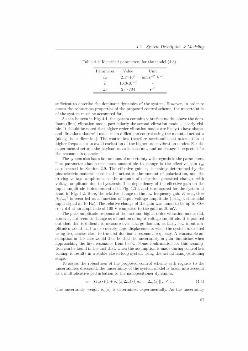
4.2. System Description & Modeling
Table 4.1: Identified parameters for the model (4.3).
Parameter Value Unitβ0 2.17·106 μm s−2 V−1
ζ 16.3·10−3 -ω0 2π · 704 s−1
sufficient to describe the dominant dynamics of the system. However, in order toassess the robustness properties of the proposed control scheme, the uncertaintiesof the system must be accounted for.
As can be seen in Fig. 4.1, the system contains vibration modes above the dom-inant (first) vibration mode, particularly the second vibration mode is clearly visi-ble. It should be noted that higher-order vibration modes are likely to have shapesand directions that will make them difficult to control using the mounted actuator(along the x-direction). The control law therefore needs sufficient attenuation athigher frequencies to avoid excitation of the higher order vibration modes. For theexperimental set-up, the payload mass is constant, and no change is expected forthe resonant frequencies.
The system also has a fair amount of uncertainty with regards to the parameters.The parameter that seems most susceptible to change is the effective gain ea,as discussed in Section 2.9. The effective gain ea is mainly determined by thepiezoelectric material used in the actuator, the amount of polarization, and thedriving voltage amplitude, as the amount of deflection generated changes withvoltage amplitude due to hysteresis. The dependency of the effective gain on theinput amplitude is demonstrated in Fig. 1.2b, and is measured for the system athand in Fig. 4.2. Here, the relative change of the low-frequency gain K = ea/k =β0/ω0
2 is recorded as a function of input voltage amplitude (using a sinusoidalinput signal at 10 Hz). The relative change of the gain was found to be up to 80%≈ -2 dB at an amplitude of 100 V compared to the gain at 50 mV.
The peak amplitude response of the first and higher order vibration modes did,however, not seem to change as a function of input voltage amplitude. It is pointedout that this is difficult to measure over a large domain, as fairly low input am-plitudes would lead to excessively large displacements when the system is excitedusing frequencies close to the first dominant resonant frequency. A reasonable as-sumption in this case would then be that the uncertainty in gain diminishes whenapproaching the first resonance from below. Some confirmation for this assump-tion can be found in the fact that, when the assumption is made during control lawtuning, it results in a stable closed-loop system using the actual nanopositioningstage.
To assess the robustness of the proposed control scheme with regards to theuncertainties discussed, the uncertainty of the system model is taken into accountas a multiplicative perturbation to the nanopositioner dynamics,
w = Gw(s)(1 + δw(s)Δw(s))ua ; ‖Δw(s)‖∞ ≤ 1 . (4.4)
The uncertainty weight δw(s) is determined experimentally. As the uncertainty
87

4. Robust Repetitive Control
0 10 20 30 40 50 60 70 80 90 1000
10
20
30
40
50
60
70
80
Input voltage amplitude (V)
Rel
ativ
e ch
ange
in g
ain
(%)
Figure 4.2: Relative change in low-frequency gain for the piezoelectric actuator dueto the input voltage amplitude (using a sinusoidal input at 10 Hz).
101 102 103
0
10
20
Mag
nitu
de (d
B)
Frequency (Hz)
Experimentally determined uncertaintyApproximation to uncertainty
Figure 4.3: Open-loop uncertainty weight δw(s), using experimental data and asover-bounding transfer-function.
apparently is very large at low frequencies, but difficult to measure over a largefrequency domain, an over-bounding transfer-function is proposed. These uncer-tainty weights are shown in Fig. 4.3.
4.3 Control Structure
The control law combines a plug-in repetitive control scheme and a proportional-integral control law as illustrated in Fig. 4.4. The PI control law is modified to in-
88

4.3. Control Structure
ua wr
nw
Wr GwCpiu
du
Wa–
v
p
Figure 4.4: System block diagram.
clude the anti-aliasing and reconstruction filters, Wa(s) and Wr(s). As was demon-strated in Section 3.4.6, this modified PI control law can be used for damping andtracking control.
4.3.1 Repetitive Control
Repetitive control tracks or rejects arbitrary periodic exogenous signals of a fixedperiod τp (s). This is achieved by embedding a model of the reference r or dis-turbance du signal into the feedback loop. The minimal and exact realization of amodel for any periodic signal with period τp is given by [224]
Γ1(s) =e−τps
1 − e−τps. (4.5)
For an appropriate initial function, this model can generate any signal with thegiven period τp, as it contains poles at s = j2πn/τp, for n = 0, 1, 2, 3, ..., ∞. How-ever, the minimal realization is not suitable for implementation on most systemssince it requires the system to be bi-proper, that is, to have relative degree n� = 0,in order to be stable in closed-loop. The remedy is to introduce a stable low-passfiler Q(s) in the model [98], i.e.,
Γ2(s) =Q(s)e−τps
1 − Q(s)e−τps.
By doing so, all the poles will shift into the complex left half-plane by an amountdepending on the frequency; thus, at higher frequencies the new pole location isfarther away from the original location than at lower frequencies. This means thatthe model is no longer exact, and importantly, the nulling property with respectto the exact model (4.5), especially at higher frequencies, is degraded.
In this work, the structure shown in Fig. 4.5a is used to implement the RCscheme, and the transfer-function is given by
Γ(s) = p
e(s) =
R(s)e−τps
1 − Q(s)e−τps. (4.6)
Two modifications have been introduced, the output filter R(s), defined below, anda modified delay τp. By modifying the time-delay in the RC block, the shift in the
89

4. Robust Repetitive Control
R(s)e– p
s
Q(s)
p
(s)
~
(a) Implementation of the plug-in repetitivecontrol law block Γ(s).
e– p
s
S(s)(1-Q(s)e p
s)
Q(s)-T(s)R(s)
r
~
~
–
–
(b) Equivalent representation of the sensitivityfunction (4.8).
Figure 4.5: Repetitive control scheme block diagrams.
poles due to Q(s) can be partially compensated for. A method for minimizing thetracking error by tuning τp is given in Section 4.4.2.
Inspecting Fig. 4.4, the closed-loop sensitivity function for the overall system is
S(s) =ε
r(s) =
11 + L(s) + L(s)Γ(s)
=1
P (s), (4.7)
where L(s) = Wa(s)Gw(s)Wr(s)Cpi(s). The stability of the closed-loop system isdetermined by the denominator P (s) = 1 + L(s) + L(s)Γ(s).
The sensitivity and complementary sensitivity function without the presence ofthe repetitive control scheme is denoted as
S(s) =ε
r(s) =
11 + L(s)
and T (s) =w
r(s) = L(s)S(s) ,
respectively. By inserting the expression for Γ(s), multiplying the numerator anddenominator of 1/P (s) by S(s), and rearranging, the sensitivity function for theclosed-loop system when adding the repetitive control scheme takes the form
S(s) =1
P (s)=
S(s)(1 − Q(s)e−τps)1 − (Q(s) − T (s)R(s))e−τps
. (4.8)
With reference to Fig. 4.5b, it can be seen that given a bounded reference r and sta-ble transfer-functions S(s) and Q(s), the small-gain theorem provides the criterionfor the stability of the closed-loop system as [98]∥∥Q(s) − T (s)R(s)
∥∥∞ < 1 , (4.9)
with |e−jτpω| = 1 ∀ ω ∈ R.The output filter R(s) is constructed as
R(s) = WT−1(s)Q(s) , (4.10)
introducing a stable all-pole filter WT (s), which provides for some flexibility inmeeting the stability criterion. Using a unity-gain low-pass filter Q(s), the simplercriterion ∥∥1 − WT
−1(s)T (s)∥∥
∞ < 1 , (4.11)
90

4.3. Control Structure
for selecting an appropriate filter WT (s) can be used. The selection of WT (s) isdescribed in Section 4.4.2.
Finally, to assess the robustness of the RC scheme, a multiplicative perturbationfor the closed-loop complementary sensitivity is used, i.e.,
w = T (s)(1 + δw(s)Δw(s))r ; ‖Δw(s)‖∞ ≤ 1 , (4.12)
where
δw(s)Δw(s) =S(s)δw(s)Δw(s)
1 + T (s)δw(s)Δw(s)⇒ |δw(jω)| ≤ |S(jω)δw(jω)| . (4.13)
Incorporating the uncertainty into the criterion (4.9), the robust stability criterion∣∣Q(jω) − T (jω)R(jω)∣∣ < 1 − ∣∣T (jω)δw(jω)R(jω)
∣∣ , (4.14)
is obtained.
4.3.2 Damping-Tacking Control
The nanopositioning stage is a lightly damped structure. Inspecting the stabilitycriterion for the RC scheme (4.9), it is expected that large peaks in the comple-mentary sensitivity function T (s) can reduce the applicable bandwidth and gain,depending on how well the output filter R(s) is able to match the inverse closed-loopdynamics T (s). Due to the inclusion of a damping and tracking control law C(s),the robustness and bandwidth possible for the overall control scheme is increased,as this control law will reduce the sensitivity to plant uncertainty, as measured bythe sensitivity function S(s), i.e., since [60, 119]
S(s) =∂T (s)/T (s)
∂Gw(s)/Gw(s)=
Gw0(s)T0(s)
∂T (s)∂Gw(s)
∣∣∣∣NOP
,
using a nominal operating point (NOP) for all the parameters in the transfer-functions.
As discussed in Section 3.4.6, a simple, effective, and robust damping and track-ing control law for a lightly damped structure can be obtained by augmenting anintegral control law by a second or higher-order low-pass filter, and optimally tun-ing the integral gain and cut-off frequency.
Since the control law is implemented in discrete time using digital-to-analog andanalog-to-digital converters, anti-aliasing and reconstruction filters must be presentin order to mitigate aliasing effects and quantization noise. By including thesefilters in the control law, an extra degree of freedom can be added for the tuningof the control law, which is the cut-off frequency of the filters. The nominal choicefor the cut-off frequency would usually be close to the Nyquist frequency if highbandwidth is required. In order to mitigate the effects of aliasing and quantizationon the system, it is desirable to choose a low cut-off frequency, but this usuallyimpacts the closed-loop stability margins negatively. However, using the dampingintegral control law, the optimal cut-off frequency turns out to be close to the first
91

4. Robust Repetitive Control
resonant frequency, which has to be well below the Nyquist frequency to avoidaliasing.
Using the proposed tuning procedure from Chapter 3 it is therefore possible toutilize the filters to good effect; damping the dominant vibration mode, reducingthe sensitivity to plant uncertainty and disturbances, and reducing the impact ofaliasing and quantization on the system. Compared to a regular integral control lawthe damping integral control law will also marginally reduce the overall noise leveldue to sensor noise, even when not considering the added noise due to quantization.
Proportional-Integral Control Law
In this Chapter, a proportional-integral (PI) control law is used, rather than theintegral control law used in Section 3.4.6, in the hopes that a slightly higher band-width can be achieved. This would be due to the increased effective stiffness in-troduced by the proportional action, which should increase the allowable integralgain.
A PI control law is typically given as
Cpi(s) =kps + ki
s, (4.15)
where kp and ki are the proportional and integral gains, respectively. The anti-aliasing and reconstruction filters are here taken to be second-order low-pass But-terworth filters
Wa(s) = Wr(s) =ωc
2
s2 +√2ωcs + ωc
2, (4.16)
where ωc is the cut-off frequency. For convenience they are chosen to be identicalwhen tuning the control law. The modified PI control law is therefore
C(s) = Wa(s)Cpi(s)Wr(s) . (4.17)
Proportional Gain Margin
When applying a proportional control law
Cp(s) = kp
to the second order system (4.3), in the ideal case with perfect sensors and actua-tors, it is straight forward to verify that the closed-loop system has an unlimitedstability margin, that is, kp can be chosen arbitrarily large. The proportional actionincreases the effective stiffness of the system, and the product ζω0
3 in (3.16) willtherefore be larger, and thus proportional action should increase the allowable gainwhen combined with integral action.
However, in the presence of phase-lag, the margin for a proportional controllaw is rather limited. Considering for instance sensor dynamics in the form of thefirst-order low-pass filter with cut-off frequency ωc
Wy(s) =ωc
s + ωc, (4.18)
92

4.4. Control Scheme Tuning & Analysis
in cascade with (4.3), the margin k∗p for the combined system determined by the
Routh-Hurwitz criterion is
kp <2ζω0(ω0
2 + 2ζω0ωc + ωc2)
ωcβ0= k∗
p . (4.19)
With parameter values from Tab. 4.1, and considering the specifications for a faststate-of-the-art capacitive probe from ADE Technologies (ADE 6810), which iswell described by (4.18) with ωc = 2π · 100 rad/s, the gain is limited to kp � 40.Adding more low-pass characteristic elements degrades the limit even more, andthe increased performance due to proportional action is therefore modest.
4.4 Control Scheme Tuning & Analysis
The tuning and analysis of the damping and tracking control law and the repetitivecontrol scheme is presented below.
4.4.1 Damping & Tracking Control Law
The damping and tracking control law is as presented in Section 3.4.6, with theaddition of proportional action. As the proportional gain is limited by phase-lagdue to instrumentation, it is set to a constant, low value. The tuning procedure isthen identical with the method presented in Chapter 3.
Effects of Low-Pass Filters in the Signal Chain
The modified PI control law (4.17) has an extra degree of freedom, in the choice ofthe cut-off frequency of the filters (4.16). As discussed in Section 3.4.6, damping canbe introduced and the overall bandwidth can be increased, by adjusting the cut-offfrequency ωc. For the system used in the experimental set-up for this Chapter, thisis illustrated in Fig. 4.6a. Setting the control gains to kp = 1 and ki = k∗
i ≈ 1300,i.e., setting the PI control law gains close to the margin of stability, the eigenvalueloci of the closed-loop system is generated by varying the cut-off frequency ωc ofthe anti-aliasing and reconstruction filters.
As can be seen from the detail in Fig. 4.6b, using filters with a cut-off frequencyequal to the Nyquist frequency, ωc = ωn = 2π · 50 rad/s, the system is unstable.The Figs. 4.6a and 4.6b indicate, however, that reducing the cut-off frequency forthe filters, all eigenvalues can be moved further into the left-half plane. Minimizingthe maximum value of the real part of the eigenvalues for the closed-loop systemas a function of the cut-off frequency ωc resulted in
arg minωc∈R+/{0}
[arg maxRe(λ)∈R−
[det(A(ωc) − λI) = 0]] ≈ 2π · 584 rad/s , (4.20)
where A(ωc) is a state matrix realization for the closed-loop system for a given ωc.Thus, setting ωc = 2π · 584 rad/s, produces the fastest modes for this system withthe selected control gains.
By inspecting Figs. 4.6a and 4.6b, it is evident that by using the computedoptimal value for the cut-off frequency, the stability margins for the closed-loop
93

4. Robust Repetitive Control
Re( )
Im(
)
(a) The positive imaginary part of the com-plex conjugate eigenvalue loci for the vibrationmode in addition to the modes due to the fil-ters (4.16), and the real valued mode due to theintegral action in (4.15). The optimal root loca-tions according to (4.20) are indicated by dots.
Re( )
Im(
)
(b) Detail from the upper-right corner ofFig. 4.6a. The eigenvalue when ωc → 0 is in-dicated by a circle, ωc due to (4.20) a star,ωc = ωn a diamond shape, and ωc → +∞ asquare.
Figure 4.6: Eigenvalue loci for the closed-loop system as a function of the filtercut-off frequency ωc. The loci are symmetric about the real axis.
Table 4.2: Optimal parameters for (4.17).
Parameter Valueωc 2π·737ki 8.33·103
system will be larger. This should allow for a larger closed-loop bandwidth. Thenew stability margin is found numerically to be about 12 · k∗
i , thus reducing thecut-off frequency increases the integral gain limit significantly.
As pointed out in Section 3.4.6, the closed-loop pole locations depend on bothki and ωc, and for the PI control law, also kp. Optimal values for ki and ωc wastherefore found solving (3.15), keeping kp fixed. As different values for kp thatgenerated a stable closed-loop system did not seem to impact the bandwidth no-ticeably, this gain value was set to kp = 1. The optimal control law parameters for(4.17) with kp = 1 found when solving (3.15) are presented in Tab. 4.2.
As an example of the feasibility of the cost-function (3.14), the surface of thecost-function in a neighborhood of the optimal values is shown in Fig. 4.7. For thissystem it can be seen that the cost-function provides a smooth and convex surface,and that the solution of (3.15) for a reasonable domain of control law parametersis unique.
It might also be interesting to compare the optimal tuning with a nominaltuning for the control law (4.17). A nominal tuning of the anti-aliasing and recon-struction filters corresponds to using ωc = ωn, i.e., the Nyquist frequency. Tuningthe PI control law for maximum bandwidth in this case requires the highest possi-ble gain for the proportional and integral term, but due to the undamped vibration
94

4.4. Control Scheme Tuning & Analysis
80008100
82008300
84008500
86008700
710720
730740
750760
770
27.7
27.8
27.9
kifc
J C(k
i,c)
Figure 4.7: Surface of the cost-function (3.14). Here, ωc = 2πfc.
mode, high gain provides little robustness, and from Fig. 4.6b it can be seen thatthe system is unstable for ωc = ωn and ki ≈ k∗
i . Using the control law parametersfrom Tab. 4.2, a gain margin of ΔK = 5.81 dB and a phase margin of Ψ = 61.6◦
is found for the loop transfer-function. To obtain similar robustness properties, acomparable gain and phase margin when using ωc = ωn is found for kp = 1 andki = 650, which yields ΔK = 5.18 dB and Ψ = 96.3◦.
The resulting frequency responses for sensitivity and complementary sensitivityfunctions for the two control law configurations are displayed in Figs. 4.8a and 4.8b.As can be seen from Fig. 4.8a, the optimal tuning very effectively attenuates theresonant peak, from 18 dB in the nominal case, to 0.88 dB in the optimal case.From Fig. 4.8b it can be seen the there is a significant increase in closed-loopbandwidth; from approximately 13 Hz in the nominal case to approximately 110Hz in the optimal case.
Due to the increased bandwidth, the effect of input disturbances du on theoutput are reduced. The effects can be measured by the input sensitivity func-tion (3.11), i.e., S(s), which provides the amount of attenuation of input distur-bances du to the input ua. By inspection the response of S(s) in Fig. 4.8b, it canbe seen that the suppression of external disturbances is in general better for theoptimally tuned control law. Disturbances will have a higher degree of suppressionat lower frequencies, but less suppression in a narrow band close to the dominantresonant peak. Due to the restriction posed by the Bode sensitivity integral, thereis no suppression outside of the bandwidth of the control law.
95

4. Robust Repetitive ControlM
agni
tude
(dB
)
3
Phas
e (d
eg)
Frequency (Hz)
Nominal tuningOptimal tuning
(a) Complementary sensitivity function T (s).
Mag
nitu
de (d
B)
Phas
e (d
eg)
Frequency (Hz)
Nominal tuningOptimal tuning
(b) Sensitivity function S(s).
Figure 4.8: Amplitude and phase responses, using nominal and optimal tuning.
Noise Performance
With regards to sensor noise performance, the transfer-function from sensor noiseto displacement is measured by (3.9), i.e., −T (s). As an example, the approximateeffect of the displacement sensor noise can be evaluated. The sensor used has abandwidth of 100 kHz, and the root-mean-square (RMS) noise is measured to beless than 2.5 nm. Assuming that the noise spectrum is fairly flat, the spectraldensity of the noise is √
Snw(jω) ≈ 7.9 pm/
√Hz .
Computing the RMS value of the noise response for −T (s), i.e.,
σw =√
Snw · ‖ − T (s)‖2 ,
for both the nominally and optimally tuned control law, provides an estimate ofthe RMS position noise due to sensor noise. It turns out to be σw = 0.34 nm forthe nominal tuning, and σw = 0.31 nm for the optimal tuning. Thus, even thoughthe bandwidth of the control law is increased by about an order of magnitude, thenoise contribution due to sensor noise is slightly decreased.
Robustness
The robustness of the modified PI control law with regards to the uncertaintiesdisplayed in Fig. 4.3 is determined. The criterion [206]
‖δw(s)T (s)‖∞ < 1 = 0 dB (4.21)
is evaluated, and the results are shown in Fig. 4.9. As can be seen, the controllaw allows for very large uncertainty in high-frequency dynamics. This means thatthe presence of higher order modes will not interfere with the stability. If thevibration modes above the first mode should be more closely spaced and havehigher peak magnitudes than what is the case for the system at hand, anti-aliasingand reconstruction filters with a higher roll-off rate can be used. It should be
96

4.4. Control Scheme Tuning & Analysis
101 102 103
0M
agni
tude
(dB
)
Frequency (Hz)
|wG(s)T(s)| using experimental uncertainty|wG(s)T(s)| using approximation to uncertainty
Figure 4.9: Evaluation of robust stability criterion |δw(jω)T (jω)| for the modifiedPI control law.
noted that the nominal tuning do not satisfy (4.21) when using the over-boundinguncertainty weight, due to the presence of the undamped resonant peak, thus thesuggested gain margin in Section 4.4.1 is not sufficient in this case.
4.4.2 Repetitive Control Law
Choosing R(s) and Q(s)
The repetitive control scheme has inherent robustness against plant uncertaintydue to the nulling property. However, robust tracking performance is not the sameas robust stability. Considering the stability criterion for the repetitive controllaw (4.11), the ideal choice for the included filter would be WT (s) = T (s), asthis would produce the minimum of the norm (4.11). As such, a sufficient choicefor WT (s) would be a filter that matches T (s) sufficiently to meet the stabilitycriterion. The filter WT (s) should be of minimal order, to reduce computationalcomplexity, and the specific choice of the filter can also provide some flexibility inmeeting the robust stability criterion (4.14).
The complementary sensitivity function T (s) has seven poles and one zero, andthus has relative degree n� = 6. By inspection of Figs. 4.8a and 4.8b one can inferthat the complementary sensitivity function has a response that closely resemblesa sixth-order all-pole low-pass filter. In order to minimize the order of WT (s), thezero in T (s) can be neglected.
Due to the frequency response of T (s), WT (s) is chosen to be a sixth-orderButterworth filter with DC-gain 1/kT , and it is assumed that WT (s) ≈ T (s). Anoptimal choice for the cut-off frequency ωT and DC-gain kT for WT (s) is found
97

4. Robust Repetitive Control
0.350.4
0.450.5
0.55560
570580
590600
1
1.1
1.2
1.3
fTkT
J T(k
R,
T)
Figure 4.10: Surface of the cost-function (4.22). Here, ωT = 2πfT .
minimizing the cost-function
JT (kT , ωT ) = sup{|Q(jω) − T (jω)R(jω, ωT , kT ))|+ |T (jω)δw(jω)R(jω, ωT , kT ))| : ω ∈ R} , (4.22)
where R(jω, ωT , kT ) = WT (jω, ωT , kT )−1Q(jω). The evaluation of the cost-functionmust satisfy JT (k�
T , ωT�) < 1 in order for the system to be robustly stable. The
closed-loop uncertainty weight δw(s) for the system, using experimental data andthe overbounding approximation, are shown in Fig. 4.11. The approximation isused for the optimization.
The filter Q(s) must be chosen before performing the optimization. This is donewith consideration to the filter R(s), and chosen to be a unity-gain sixth-orderButterworth filter, such that R(s) = WT
−1Q(s) is a proper filter. By inspection ofthe frequency response in Fig. 4.1, a cut-off frequency for Q(s) is chosen in order toattenuate the second and higher order vibration modes, in order to satisfy (4.14).A cut-off frequency ωQ = 2π · 2000 rad/s provided sufficient attenuation, yieldingthe optimal values k�
T ≈ 0.45 and ωT� ≈ 2π · 580 when minimizing (4.22).
The surface of the cost-function in a neighborhood of the optimal values isshown in Fig. 4.10. As can be seen, there is a domain along a line segment, ornarrow area, where the sensitivity of the cost-function is low, and thus there areseveral values for kT and ωT that evaluate to approximately the same cost. Thismeans that the value of kT and ωT can be increased while still being robustly
98

4.4. Control Scheme Tuning & Analysis
Table 4.3: Optimal parameters for WT (s) and WQ(s).
Parameter ValuekT 0.45ωT 2π·580ωQ 2π·2000
101 102 103
0
10
20
Mag
nitu
de (d
B)
Frequency (Hz)
Figure 4.11: Closed-loop uncertainty weight δw(s), using experimental data and asan over-bounding transfer-function.
stable. Adjusting kT and ωT impacts the transient response and the specific formof the closed-loop frequency response. There could therefore be other values ofthese parameters that provide faster convergence or less sensor noise contribution.Choosing WT (s) = T (s) will essentially eliminate the transient response, since ityields P (s) = 1 in (4.8), but it will not impact the stationary response as long asthe reference signal conforms to the internal model.
The evaluation of (4.14) is shown in Fig. 4.12, and demonstrates that the choiceof ωQ and the optimal values for kT and ωT indeed provide robust stability of theclosed-loop system.
It should be noted at this point that the choice of WT (s) = T (s) does notprovide as good results when evaluating (4.14). In this case the cut-off frequencymust be ωQ < 2π · 1700 to be robustly stable. As the bandwidth of Q(s) is oneof the most important factors for obtaining good reference trajectory tracking, ωQ
should be as high as possible.It should also be noted that (4.14) appears to provide a somewhat conservative
result. By tuning the system manually, it is possible to increase the cut-off frequencyfor Q(s) to ωQ = 2π · 3000, while decreasing the DC-gain to kT = 0.275, keepingωT that same. This tuning violates (4.14), but provides a larger bandwidth for theRC scheme, and thus increases the tracking performance.
99

4. Robust Repetitive Control
101 102 103
0M
agni
tude
(dB
)
Frequency (Hz)
|Q(j ) R(j )|) w (j )) R(j )|
using experimental uncertainty) w (j )) R(j )|
using approximation to uncertainty
Figure 4.12: Evaluation of stability criteria (4.9) and (4.14).
Tuning of the Time-Delay
Inspecting the sensitivity function (4.8), note that the numerator contains theexpression
Z(s) = 1 − Q(s)e−τps .
Had the exact model (4.5) been used, the expression would have been
Z(s) = 1 − e−τps ,
which evaluates to
L−1 [(1 − e−τps)r(s)]= r(t) − r(t − τp) = 0 ∀ t > τp ,
when r(t) = 0 ∀ t < 0 and r(t) = r(t + τp). Thus, disregarding the initial valueresponse of the system, the reference signal is perfectly nulled in the error after oneperiod τp of the reference signal, and perfect tracking is obtained. For the actualimplementation
L−1 [(1 − Q(s)e−τps)r(s)]= r(t) − r(t − τp)
where r(t) = Q(t) ∗ r(t) �= r(t), is used. Since the filter Q(s) alters the referencesignal, perfect tracking can not be obtained. The residual error depends both onQ(s) and the time-delay τp, and thus, a simple method to improve the trackingperformance is to adjust τp.
By filtering the intended reference signal by Z(s), it is possible to numericallyevaluate the amount of suppression, or nulling, of the reference signal. By adjust-ing τp = τp − τδ by varying τδ, an optimal τδ that produces the best trackingperformance can be found, i.e., minimizing
J(τδ) =∥∥L−1 (Z(s, δ)
) ∗ r(t)∥∥
2 , t ∈ [τpm, τp(m + 1)] ,
100

4.4. Control Scheme Tuning & Analysis
Table 4.4: Optimal values for τδ at various reference frequencies for Q(s) withωQ = 2π · 2000 rad/s.
fp τδ
25 Hz 3.07709 · 10−4 s
50 Hz 3.08076 · 10−4 s
100 Hz 3.08384 · 10−4 s
200 Hz 3.08982 · 10−4 s
400 Hz 3.09129 · 10−4 s
103
0
Mag
nitu
de (d
B)
Frequency (Hz)
)|ideal
)|nominal
)|~
Figure 4.13: Zero locations for different configurations of Z(s), using τp = 1/200 s.
where τδ ∈ (0, τp), and m is a positive integer to make sure τpm is large enough forthe transient response of Q(s) to have died out. Results are presented in Tab. 4.4.Note that it is possible to implement time-delays with a non-integer multiple ofthe sampling time using Thiran approximation [132].
An example of the effect on the zero locations of Z(s) is shown in Fig. 4.13.Here the amplitude response of Z(s) is computed with and without the filter Q(s),for τp and τp, using fp = 200 Hz.
101

4. Robust Repetitive Control
Noise Performance
Sensor noise performance for the case when including the RC scheme in the feed-back loop, can be measured using −T (s), where
T (s) =L(s) + L(s)Γ(s)
1 + L(s) + L(s)Γ(s)=
T (s)(1 − (Q(s) − R(s))e−τps)1 − (Q(s) − T (s)R(s))e−τps
.
As in the example for the modified PI control law, a noise spectral density of√Snw
(jω) ≈ 7.9 pm/√Hz ,
is assumed. The RMS value of the noise response for −T (s) is then
σw =√
Snw· ‖ − T (s)‖2 .
This value depends on the time-delay value τp, but upper and lower bounds for theamplitude response that are independent of the time-delay value can be found as∣∣1 − |Q(jω) − R(jω)| ∣∣
1 +∣∣Q(jω) − T (jω)R(jω)
∣∣ ≤ |T (jω)| ≤ 1 + |Q(jω) − R(jω)|∣∣1 − ∣∣Q(jω) − T (jω)R(jω)∣∣ ∣∣ .
An example of the power spectral density for −T (s) is shown in Fig. 4.14, usingτp = 1, together with the upper and lower bound, and the power spectral densityfor −T (s).
The RMS value of the noise response for the power spectral density in Fig. 4.14for −T (s) can be computed to be σw = 0.48 nm, by numerically integrating the areaunder the curve and taking the square root. This means that the noise contributionis larger when adding the RC scheme, compared to when using the modified PIcontrol law alone.
Numerically integrating the area under the bounds and taking the square root,yields 1.5 nm for the upper bound and 0.098 nm for the lower bound. The boundsare therefore not very tight.
Assuming that R(s) = T −1(s)Q(s), the complementary sensitivity function is
T (s) = T (s) + Q(s)S(s)e−τps ,
and a bound for the H2-norm can be found as
‖−T (s)‖2 = ‖T (s)‖2 ≤ ‖T (s)‖2 + ‖Q(s)S(s)‖2 .
Another approximate estimate can therefore be found computing√Snw · (‖T (s)‖2 + ‖Q(s)S(s)‖2
),
which yields σw = 0.90 nm in this case.If the bandwidth of Q(s) is significantly larger than T (s), and if |T (jω)| +
|S(jω)| ≈ 1, the spectral density can be seen to be dominated by the filter Q(s).Thus, yet another approximation for the noise contribution be found computing√
Snw · ‖Q(s)‖2 ,
which yields σw = 0.50 nm in this case.
102

4.4. Control Scheme Tuning & Analysis
101 102 103 10410
10
10
10
10
10
(Hz)
(μm
2 /Hz)
PI+RCPIPI+RC Upper BoundPI+RC Lower Bound
Figure 4.14: Power spectral densities for −T (s) and −T (s), with upper and lowerbounds.
Summary of the Tuning Procedure
The tuning procedure can be summarized to the following steps:1. Identify the parameters of the model (4.3) for the dominant vibration mode
in the system.2. Construct the uncertainty weight δw(s) in (4.4).3. Find the optimal parameters for the anti-aliasing and reconstruction filters
and the integral control law by solving (3.15).4. Verify the stability of the modified PI control law using (4.21). If non-modeled
high-frequency dynamics is a problem, anti-aliasing and reconstruction filterswith a higher roll-off rate should be used.
5. Compute the uncertainty weight δw(s) using (4.13).6. Choose an appropriate filter WT (s) with the cut-off frequency ωT and the
DC-gain kT as tunable parameters, using, e.g., (4.11).7. Chose an appropriate order and cut-off frequency ωQ for the unity-gain
low-pass filter Q(s). The cut-off frequency must be chosen in order to pro-vide sufficient attenuation of high-frequency dynamics. The filter R(s) =WT (s)−1Q(s) should be proper.
8. Find the optimal values for ωT and kT using (4.22).
103

4. Robust Repetitive Control
9. Verify the stability of the overall control scheme using (4.14). If high-frequencydynamics is a problem, reduce the cut-off frequency ωQ.
4.5 Experimental Results & Discussion
To validate the performance and robustness of the proposed control scheme, exper-iments were performed for tracking a modified triangle-wave reference signal, usingdifferent fundamental frequencies and amplitudes, as well as tuning parameters forthe PI control law and the combined PI and RC control law.
4.5.1 Description of the Experimental System
The experimental set-up consisted of a dSPACE DS1103 hardware-in-the-loop sys-tem, a ADE 6810 capacitive gauge and ADE 6501 capacitive probe from ADETechnologies, a Piezodrive PDL200 voltage amplifier, the custom-made long-rangeserial-kinematic nanopositioner (see Fig. 2.3), two SIM 965 programmable filtersand a SIM983 scaling amplifier from Stanford Research Systems. The capacitivemeasurement has a sensitivity of ks = 1/5 V/μm and the voltage amplifier hasa gain of 20 V/V. With the DS1103 board, a sampling time of Ts = 1 · 10−5 s(fs = 100 kHz) was used for all the experiments. For numerical integration, afourth-order Runge-Kutta scheme [62] was used.
The scaling amplifier was used to modify the sensitivity of the capacitive gaugein order to maximize the resolution obtained from the analog-to-digital converter.The sensitivity was set to ks = 3.25/5 V/μm for the largest reference signal am-plitude, and ks = 6.5/5 V/μm for the smallest reference signal amplitude. Thequiescent noise in the system was measured. The measured time-series and powerspectral density (PSD) estimates for the two sensitivity settings are presented inFig. 4.15 for reference. The noise floor is determined by the performance of theanalog-to-digital converter (ADC), and for an ideal ADC the noise spectral den-sity due to quantization is determined as [145, 175]
Sq(jω) =1fs
Δqr2
6, (4.23)
where the quantization resolution Δqr is determined by Δqr = Radc/2nb whereRadc is the range and nb is the word length (number of bits) of the ADC. Thehardware-in-the-loop system used has a range of Radc = 20 V and a word lengthof nb = 16 bits. The signal-to-noise ratio is better than 83 dB, which means that,depending on the method used [3, 145, 175], the effective number of bits is between13 and 15. Assuming the best case scenario of nb = 15 effective bits, the noise floorSnf (jω) = ks
2Sq(jω) should be -118 dB/Hz for the sensitivity setting for largesignals and -124 dB/Hz for the sensitivity setting for small signals. Consideringagain Fig. 4.15b, it is reasonable to assume that the noise contribution is dominatedby quantization noise above 1 kHz.
104

4.5. Experimental Results & Discussion
0 0.005 0.01 0.015 0.02 0.025 0.03 0.035 0.04 0.045 0.05
0
0.5
1
1.5
Time (s)
Def
lect
ion
(nm
)
Sensitivity @ 3.25/5 V/μm, Max: 2.10 nm, RMS: 0.509 nmSensitivity @ 6.50/5 V/μm, Max: 1.25 nm, RMS: 0.368 nm
(a) Time-series.
0 500 1000 1500 2000 2500Frequency (Hz)
Pow
er/fr
eque
ncy
(dB
/Hz)
(b) Power spectral density estimate.
Figure 4.15: Measured quiescent noise from displacement sensor filtered by theanti-aliasing filter.
4.5.2 Results
Two results from the experiments are presented in Fig. 4.16 and 4.18. The firstresult is for scanning at 25 Hz when using a nominal and optimal tuning of thePI control law. As the nominal tuning proposed in Section 4.4.1 turned out therender an unstable control law, it was necessary to reduce the nominal integralgain to ki = 525. Fig. 4.16a displays the steady-state measured deflection signalsym = Wa(s)w, and Fig. 4.16b shows the power spectral density (PSD) estimateof the measured steady-state error signals e = Wa(s)r − ym. The second result iswhen scanning at 200 Hz using the optimally tuned PI control law and the repeti-tive control law. Fig. 4.18a displays the initial transient response of the measureddeflection and error, Fig. 4.18b the steady-state measured deflection and Fig. 4.18dthe steady-state measured error. Fig. 4.18c is a PSD estimate of the steady-stateerror. In Fig. 4.18e the steady-state control input u is shown. A summary of all theexperiments performed are presented in Tab. 4.5.
The results of the experiments in Tab. 4.5 are rated using both the maximumerror (ME) and the root-mean-square error (RMSE), both in absolute terms withrespect to the measured deflection, and relative to the maximum value of thereference signal for ME, and the RMS value of the reference signal for RMSE.
4.5.3 Discussion
Considering Fig. 4.16a and the results for the PI control law in Tab. 4.5, it isimmediately apparent that the bandwidth is increased, as the tracking error forthe 25 Hz fundamental frequency signal decreases from 80% when using the nominaltuning to 12% when using the optimal tuning. From Fig. 4.16b, it is also evidentthat damping is introduced, as the prominent peak appearing around 750 Hz1, dueto the mechanical resonance, is reduced by about 40 dB/Hz.
1The frequency resolution is low due to windowing of the data prior to computing the powerspectral density.
105
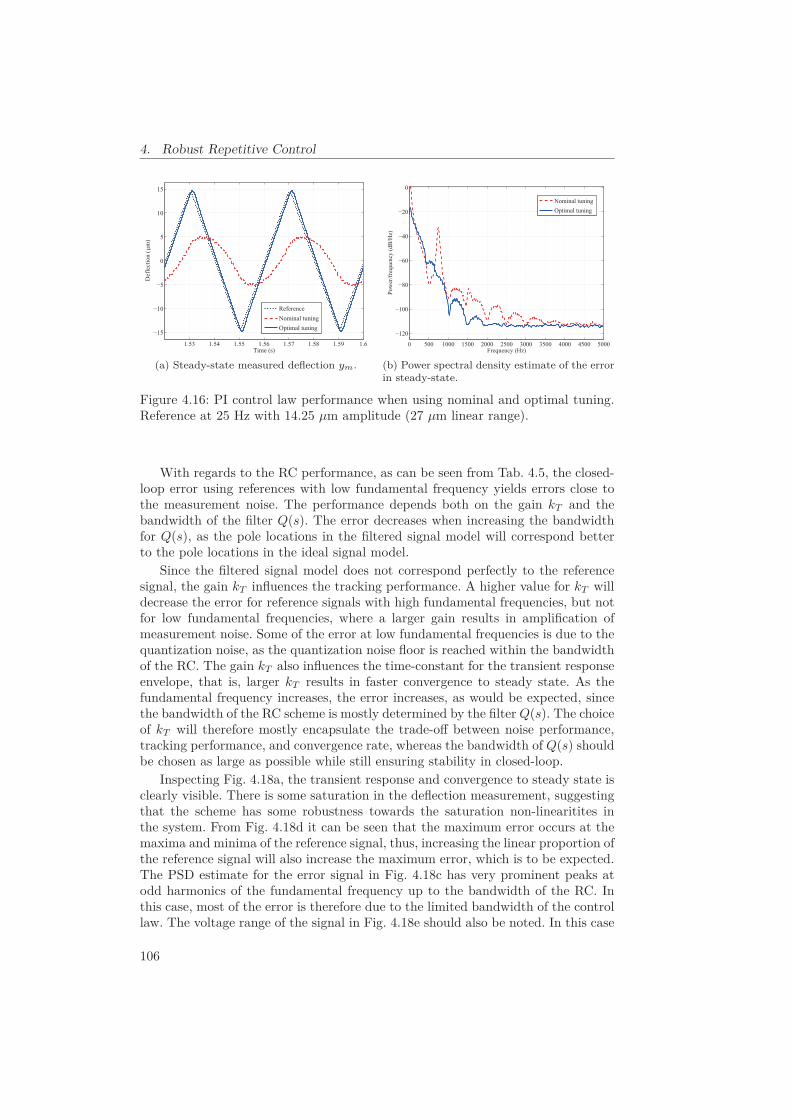
4. Robust Repetitive Control
1.53 1.54 1.55 1.56 1.57 1.58 1.59 1.6
5
15
Time (s)
Def
lect
ion
(μm
)
ReferenceNominal tuningOptimal tuning
(a) Steady-state measured deflection ym.
0 500 1000 1500 2000 2500 3000 3500 4000 4500 5000
0
Frequency (Hz)
Pow
er/fr
eque
ncy
(dB
/Hz)
Nominal tuningOptimal tuning
(b) Power spectral density estimate of the errorin steady-state.
Figure 4.16: PI control law performance when using nominal and optimal tuning.Reference at 25 Hz with 14.25 μm amplitude (27 μm linear range).
With regards to the RC performance, as can be seen from Tab. 4.5, the closed-loop error using references with low fundamental frequency yields errors close tothe measurement noise. The performance depends both on the gain kT and thebandwidth of the filter Q(s). The error decreases when increasing the bandwidthfor Q(s), as the pole locations in the filtered signal model will correspond betterto the pole locations in the ideal signal model.
Since the filtered signal model does not correspond perfectly to the referencesignal, the gain kT influences the tracking performance. A higher value for kT willdecrease the error for reference signals with high fundamental frequencies, but notfor low fundamental frequencies, where a larger gain results in amplification ofmeasurement noise. Some of the error at low fundamental frequencies is due to thequantization noise, as the quantization noise floor is reached within the bandwidthof the RC. The gain kT also influences the time-constant for the transient responseenvelope, that is, larger kT results in faster convergence to steady state. As thefundamental frequency increases, the error increases, as would be expected, sincethe bandwidth of the RC scheme is mostly determined by the filter Q(s). The choiceof kT will therefore mostly encapsulate the trade-off between noise performance,tracking performance, and convergence rate, whereas the bandwidth of Q(s) shouldbe chosen as large as possible while still ensuring stability in closed-loop.
Inspecting Fig. 4.18a, the transient response and convergence to steady state isclearly visible. There is some saturation in the deflection measurement, suggestingthat the scheme has some robustness towards the saturation non-linearitites inthe system. From Fig. 4.18d it can be seen that the maximum error occurs at themaxima and minima of the reference signal, thus, increasing the linear proportion ofthe reference signal will also increase the maximum error, which is to be expected.The PSD estimate for the error signal in Fig. 4.18c has very prominent peaks atodd harmonics of the fundamental frequency up to the bandwidth of the RC. Inthis case, most of the error is therefore due to the limited bandwidth of the controllaw. The voltage range of the signal in Fig. 4.18e should also be noted. In this case
106

4.5. Experimental Results & Discussion
0 0.1 0.2 0.3 0.4 0.5 0.6
0
10
Time (s)
Def
lect
ion
(μm
)
0 0.1 0.2 0.3 0.4 0.5 0.6
0
1
Time (s)
Erro
r (μm
)
(a) Initial transient measured deflection ym and measured error ε.
0.09 0.1 0.11 0.12 0.13 0.14 0.15 0.16
0
5
10
15
Time (s)
Def
lect
ion
(μm
)
ReferenceMeasurement
(b) Steady-state measured deflection ym.
0 1000 2000 3000 4000 5000 6000 7000 8000 9000 10000Frequency (Hz)
Pow
er/fr
eque
ncy
(dB
/Hz)
(c) Power spectral density estimate of the errorin steady-state.
0.09 0.1 0.11 0.12 0.13 0.14 0.15 0.16
0
5
x 10
Erro
r (μm
)
Time (s)0.09 0.1 0.11 0.12 0.13 0.14 0.15 0.16
0
0.05
Erro
r (%
)
ME: 0.00699 μm (0.0491%), RMSE: 0.0017 μm (0.0197%)
(d) Steady-state measured error ε.
0.09 0.1 0.11 0.12 0.13 0.14 0.15 0.16
0
20
40
60
Time (s)
Vol
tage
(V)
(e) Steady-state input voltage u.
Figure 4.17: Reference at 25 Hz with 14.25 μm amplitude (27 μm linear range).
107

4. Robust Repetitive Control
0 0.01 0.02 0.03 0.04 0.05 0.06 0.07
0
10
Time (s)
Def
lect
ion
(μm
)
0 0.01 0.02 0.03 0.04 0.05 0.06 0.07
0
10
Time (s)
Erro
r (μm
)
(a) Initial transient measured deflection ym and measured error ε.
0.011 0.012 0.013 0.014 0.015 0.016 0.017 0.018 0.019 0.02
0
5
10
15
Time (s)
Def
lect
ion
(μm
)
ReferenceMeasurement
(b) Steady-state measured deflection ym.
0 1000 2000 3000 4000 5000 6000 7000 8000 9000 10000Frequency (Hz)
Pow
er/fr
eque
ncy
(dB
/Hz)
(c) Power spectral density estimate of the errorin steady-state.
0.011 0.012 0.013 0.014 0.015 0.016 0.017 0.018 0.019 0.02
0
0.1
Erro
r (μm
)
Time (s)0.011 0.012 0.013 0.014 0.015 0.016 0.017 0.018 0.019 0.02
0
0.5
1
Erro
r [%
]
ME: 0.116 μm (0.864%), RMSE: 0.0472 μm (0.551%)
(d) Steady-state measured error ε.
0.011 0.012 0.013 0.014 0.015 0.016 0.017 0.018 0.019 0.02
0
20
40
60
80
100
Time (s)
Vol
tage
(V)
(e) Steady-state input voltage u.
Figure 4.18: Reference at 200 Hz with 14.25 μm amplitude (27 μm linear range).
108

4.6. Conclusions
Table 4.5: Norms of the measured error ε in steady-state, using various configura-tions and reference signals. fp and 2λ denotes the fundamental frequency and linearrange, respectively, of the reference signal. Entries marked with “†” are obtainedusing a tuning that violates the robust stability criterion (4.14).
fp
(Hz)2λ(μm) kT
fQ
(kHz)ME abs.(μm)
ME rel.(%)
RMSEabs.(μm)
RMSErel.(%)
When using nominally tuned PI control law25 27.0 – – 11 80 7.1 83
When using optimally tuned PI control law25 27.0 – – 1.7 12 1.0 12200 27.0 – – 16 120 9.8 110
When using PI control law and repetitive control law25 13.5 0.450 2 0.0034 0.048 0.00067 0.01625 13.5 0.100 3† 0.0023 0.032 0.00053 0.01225 13.5 0.275 3† 0.0036 0.050 0.00091 0.02125 27.0 0.350 2 0.0048 0.033 0.0011 0.01325 27.0 0.450 2 0.0072 0.050 0.0017 0.02050 27.0 0.450 2 0.011 0.077 0.0028 0.032100 27.0 0.450 2 0.031 0.22 0.010 0.12200 13.5 0.450 2 0.61 0.91 0.025 0.59200 13.5 0.275 3† 0.030 0.44 0.012 0.27200 27.0 0.450 2 0.12 0.86 0.047 0.55400 13.5 0.450 2 0.12 1.9 0.064 1.6
the full range of the amplifier, ±110 V is used, and it provides a hard limit withregards to the spectral content and the range of the reference signal, as well as thebandwidth of the control law. Increasing either one of these properties in this case,would have resulted in saturation in the amplifier.
4.6 Conclusions
It has been demonstrated through experiments that by using a damping proportional-integral control law and a well configured plug-in repetitive control scheme, it ispossible to achieve a maximum error of less than 1% relative to the reference signal,at reference signal frequencies exceeding 25% of the dominant resonant frequencyof a nanopositioning stage. The methods used are straight forward to implementand tune, and the overall control scheme is applicable for tracking control on flexi-ble smart structures in general. Additionally, the control scheme is computationallylight, and is therefore well suited for implementation on both microcontrollers and
109

4. Robust Repetitive Control
field-programmable-arrays. It should also be implementable using analog compo-nents and a bucket-brigade device, which could be beneficial with regards to quan-tization noise, which is the dominant source of noise in the system. The proposedscheme can also be implementable on existing hardware configurations for nanopo-sitioning, as it requires very small, or no, modifications to a standard configuration.
110

Part III
Adaptive Control
111


Chapter 5
Online Parameter Identification
5.1 Introduction
When applying damping control, or damping and tracking control, to highly reso-nant flexible structures, it is possible to find optimal control law parameters thatwill maximize the introduced damping, as was demonstrated in Chapter 3. Find-ing the optimal control law parameters requires knowledge of the dynamics of theflexible structure at hand. The approach in Chapter 3 was to use an accurate de-scription of the dynamics obtained from frequency response data, and the optimalcontrol law parameters was found using an optimization scheme incorporating thesedata. This would also be the typical approach taken when using H∞-synthesis.
In some applications, system parameters can be expected to change during op-eration. As discussed in Section 1.2.1 and Chapter 2, parameter uncertainty innanopositioning devices is experienced in the effective gain for the piezoelectricactuator and the resonant frequencies. The effective gain is influenced by the pres-ence of hysteresis, actuator temperature and age, as well as payload mass. Themain cause of change in resonant frequencies is due to variable payload mass. Inscanning probe microscopy applications, the most severe example of this is whenthe sample must be contained in, e.g., liquid cells with heating elements [85].
Due to changing system model parameters, feed-forward and feedback controllaw parameters should be adjusted accordingly to maintain optimal performance.An example of the reduction in performance that can occur if the system modelparameters does not correspond to the actual system was discussed in Section 2.4,where a set of hysteresis model parameters were applied under different conditionsthan what they where found for, resulting in poor reference trajectory tracking.
It is apparent that control schemes for such devices can benefit from some formof online adaptation or learning to maintain optimal performance, or even stability,during operation.
For periodic reference trajectories, this has been studied on the form of iterativelearning control (see Sections 1.3 and 4.1). Here, the method often relies on batchprocessing of measurement data, as the implementation of iterative learning con-trol methods can be very computationally demanding, but can provide practicallyperfect reference tracking. Feedback in the form of repetitive control, as discussed
113

5. Online Parameter Identification
in Chapter 4, also provides a method which is asymptotically invariant to plantuncertainties for periodic exogenous signals.
Standard online parameter identification techniques [111, 204], however, doesnot seem to have been studied extensively for experimental systems that canbe modeled as mass-spring-damper systems. Such techniques include the gradi-ent method, recursive least-squares method, and the extended Kalman filter. Oneexample applying the extended Kalman filter can be found for a geometric mass-spring system in [90].
Parameter identification with good accuracy is immediately applicable whenusing feed-forward model inversion [44], and for model reference adaptive con-trol [111], and could contribute to better performance for reference trajectorytracking and disturbance rejection for arbitrary signals.
5.1.1 Contributions
Two common schemes for online parameter identification are compared experimen-tally in order to assess their ability to learn the parameters for a simple second-order linear model (a mass-spring-damper model) of the vibration dynamics in ananopositioning device in open-loop. The schemes investigated are the recursiveleast-squares method (RLS) and two different versions of the extended Kalmanfilter (EKF); continuous EKF and hybrid EKF.
The main contribution is the specific choice of pre-filters for the various signalsinvolved in the identification method. It is demonstrated using measured time-series data acquired when operating a standard experimental set-up, that thesefilters have to be present in order to obtain reasonable parameter convergence.
5.1.2 Outline
The Chapter is organized as follows. The system is described in Section 5.2, in-cluding the plant model, the signal chain, and how to select the pre-filters neededto obtain parameter estimate convergence. This is followed by a description of howto apply the RLS and EKF methods to the plant model in Section 5.3. The exper-iments are described in Section 5.4, as well as implementation specific details, suchas choice of initial values and various tunable parameters. The results from theexperiments are presented in Section 5.5, followed by a discussion in Section 5.6.
5.2 System Description & Modeling
5.2.1 Mechanical Model
As has been discussed in previous Chapters, the dynamics of the flexible structureof a nanopositioning device is often adequately described by a lumped parameter,truncated linear model. The positioning stage used in the experiments is shown inFig. 2.3. This is a well-designed positioning stage which has one dominant vibra-tion mode with a mode shape that generates a piston-like motion. The governingdifferential equation for the displacement w (m) of a point on the structure is
114

5.2. System Description & Modeling
Mag
nitu
de (d
B)
3
Phas
e (d
eg)
Frequency (Hz)
Measured response w/payloadModel fitMeasured response wo/payloadModel fit
Figure 5.1: Measured frequency response for one axis of the nanopositioning stage,and the corresponding response using the model (5.2) with parameter values fromTab. 5.1, with and without payload attached to the sample platform.
thereforemw + dw + kw = fa ,
where m (kg) is the mass of the moving sample platform, d (N s m−1) is thedamping coefficient, k (N m−1) is the spring constant, and fa (N) is the forcedeveloped by the actuator. The applied force fa (N) is accurately described usingthe expression
fa = ea(ua + du) ,
where ea (N V−1) is the effective gain of the piezoelectric actuator, ua (V) is theapplied voltage, and du (V) is the disturbance generated by hysteresis and creep.The transfer-function from applied voltage to displacement is
Gw(s) =w
ua(s) =
β0
s2 + 2ζω0s + ω02 =b0
s2 + a1s + a0, (5.1)
and denoting x1 = w, the state-space formulation for the system is given as
x1 = x2x2 = −a0x1 − a1x2 + b0u,
(5.2)
where β0 = b0 = ea/m (m s−2 V−1), a0 = k/m (s−2), a1 = d/m (s−1), ζ =c/2
√mk, and ω0 = 2πf0 =
√k/m (s−1).
115

5. Online Parameter Identification
Table 5.1: Identified parameters for the model (5.2), for two payload configurations,using frequency response data.
Parameter Value Unit Parameter Value Unit1) With payload on sample platform
b0 0.808·106 μm/s2V b0/a0 0.114 μm/Va0 7.06·106 1/s2 f0 423 Hza1 77.6 1/s ζ 0.0146
2) Without payload on sample platformb0 1.07·106 μm/s2V b0/a0 0.116 μm/Va0 9.21·106 1/s2 f0 483 Hza1 86.8 1/s ζ 0.0143
The frequency response for y-axis of the positioner was recorded, with andwithout a payload of approximately 24.75 g attached to the sample platform, usingbandwidth-limited white noise excitation. The physical implementation of the twopayload configurations is shown in Fig. 5.2. The two responses are displayed inFig. 5.1. The model (5.2) was fitted to the frequency response data using theMATLAB System Identification Toolbox, and the resulting parameter values arepresented in Tab. 5.1. The response of the model (5.2) using these parameters arealso displayed in Fig. 5.1.
As can be seen, the actual response of the first vibration mode is well approxi-mated by the model. There are higher order modes in the system, and the secondvibration mode is clearly visible in Fig. 5.1. The higher order modes have fairly neg-ligible magnitude responses in comparison to the first, thus a second-order modelshould be sufficient to describe the dominant dynamics of the system. The mea-sured phase response in Fig. 5.1 is not only in the range between -180◦ and 0◦,indicating that the sensor is not perfectly co-located with the actuator.
5.2.2 Signal Chain
The complete system used in the experiments consisted of the nanopositioningstage, a reconstruction filter, an anti-aliasing filter, an amplifier, and a displacementsensor, as well as a standard hardware-in-the-loop (HIL) system. The signal chainis shown schematically in Fig. 5.3.
The sampling frequency used was 10 kHz. The anti-aliasing and reconstructionfilters, Wa(s) and Wr(s) were configured as second-order low-pass Butterworthfilters with conservative cut-off frequencies at 1 kHz. The amplifier, given the ca-pacitive load of the piezoelectric actuator, provided a bandwidth of approximately10 kHz, and the displacement sensor was configured with a bandwidth of 100 kHz.The dynamic response of both the amplifier and the capacitive probe can accuratelybe described using a first-order low-pass filter.
As the reconstruction and anti-aliasing filters noticeably impact the observeddynamics, these were taken into account when generating the input signal fed to
116

5.2. System Description & Modeling
(a) With payload attached. (b) Without payload attached.
Figure 5.2: Payload configurations.
ymuWr Wamp Gw Wcap Wa
PositioningStage
CapacitiveProbe
Anti-aliasingFilter
ReconstructionFilter
Amplifier
ua w
Figure 5.3: Signal chain for the overall system.
Wp
Wr·Wa·Wp
ym
u
m^Identification
scheme
Figure 5.4: Signals fed to identification schemes.
the identification schemes, as shown in Fig. 5.4. This ensured that the input signalu would match the change in gain and phase introduced by these filters in themeasured signal ym. The effects of the amplifier and the displacement sensor wereneglected, as it would be impossible to implement replicas of these filters digitallywith the chosen sampling frequency.
To improve the results obtained from the parameter identification schemes, apre-filter, Wp(s), was used. This was chosen with consideration to the sensitivity
117

5. Online Parameter Identification
functions for the parameters of the model. For a transfer-function, i.e., Gw(s), theBode sensitivity function with respect to some parameter θ, is defined as
SGw(s)θ
Δ=∂Gw(s)/Gw(s)
∂θ/θ=
θ0
Gw(s)0∂Gw(s)
∂θ
∣∣∣∣NOP
,
using a nominal operating point (NOP) for all the parameters in the transfer-function [119].
The sensitivity functions for the parameters b0, a0, and a1 in the system model(5.2), using the parameters found for the system with payload as the NOP, aredisplayed in Fig. 5.5. Most notably, the parameter related to damping, a1, has verylittle impact on the observed output at low and high frequencies. For parameteridentification it is considered good practice to concentrate signal power in thefrequency domains that contain peaks in the sensitivity functions. This is done inorder to maximize the information content of the signals used, i.e., some norm onthe Fisher information matrix [144].
The pre-filter was chosen to be a band-pass filter, using a first-order high-passfilter with a lower cut-off frequency of flc = 100 Hz, and a resonant second-orderlow-pass filter, with a natural frequency of
fc = 450 ≈ 483 + 4232
Hz,
and a damping ratio of ζ = 0.1, thus amplifying the frequency content close to theresonant peaks of the two configurations (with and without payload):
Wp(s) =s
s + 2πflc
(2πfc)2
s2 + 2ζπfcs + (2πfc)2(5.3)
When applying the RLS method, numerical first and second derivatives of thedisplacement signal are needed. In order to generate proper transfer-functions forfiltering the displacement signal, the low-pass filter should be at least second-order.To keep the order of the pre-filter at a minimum, the high-pass filter was chosento be first-order, and the low-pass filter second-order.
5.3 Identification Schemes
5.3.1 Application of the Recursive Least-Squares Method
The recursive least-squares (RLS) method summarized in Section D.1. Here thespecific application of the method to the system model (5.1) is described.
The model (5.1) can be put on the form
w + a1w + a0 = b0ua ⇒ z = θTϕ
where a parameter vector θ can be found as
θ = [b0, a1, a0]T ,
118
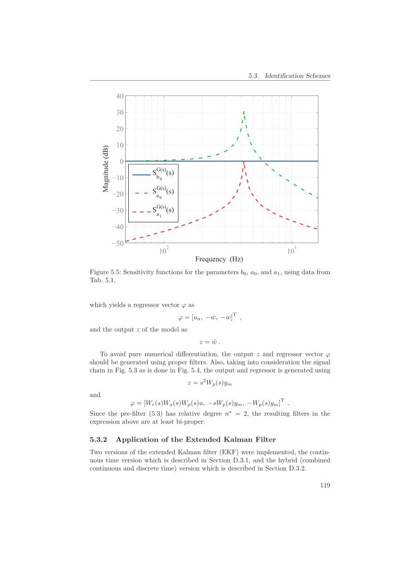
5.3. Identification Schemes
102 103
0
10
20
30M
agni
tude
(dB
)
Frequency (Hz)
SG(s)b 0
(s)
SG(s)a0
(s)
SG(s)a1
(s)
Figure 5.5: Sensitivity functions for the parameters b0, a0, and a1, using data fromTab. 5.1.
which yields a regressor vector ϕ as
ϕ = [ua, −w, −w]T ,
and the output z of the model as
z = w .
To avoid pure numerical differentiation, the output z and regressor vector ϕshould be generated using proper filters. Also, taking into consideration the signalchain in Fig. 5.3 as is done in Fig. 5.4, the output and regressor is generated using
z = s2Wp(s)ym
andϕ = [Wr(s)Wa(s)Wp(s)u, −sWp(s)ym, −Wp(s)ym]T .
Since the pre-filter (5.3) has relative degree n� = 2, the resulting filters in theexpression above are at least bi-proper.
5.3.2 Application of the Extended Kalman Filter
Two versions of the extended Kalman filter (EKF) were implemented, the contin-uous time version which is described in Section D.3.1, and the hybrid (combinedcontinuous and discrete time) version which is described in Section D.3.2.
119
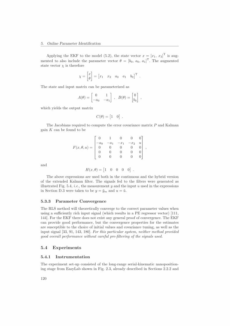
5. Online Parameter Identification
Applying the EKF to the model (5.2), the state vector x = [x1, x2]T is aug-mented to also include the parameter vector θ = [b0, a0, a1]T. The augmentedstate vector χ is therefore
χ =[xθ
]=[x1 x2 a0 a1 b0
]T.
The state and input matrix can be parameterized as
A(θ) =[0 1
−a0 −a1
], B(θ) =
[0b0
],
which yields the output matrix
C(θ) =[1 0
].
The Jacobians required to compute the error covariance matrix P and Kalmangain K can be found to be
F (x, θ, u) =
⎡⎢⎢⎢⎢⎣
0 1 0 0 0−a0 −a1 −x1 −x2 u0 0 0 0 00 0 0 0 00 0 0 0 0
⎤⎥⎥⎥⎥⎦ ,
andH(x, θ) =
[1 0 0 0 0
].
The above expressions are used both in the continuous and the hybrid versionof the extended Kalman filter. The signals fed to the filters were generated asillustrated Fig. 5.4, i.e., the measurement y and the input u used in the expressionsin Section D.3 were taken to be y = ym and u = u.
5.3.3 Parameter Convergence
The RLS method will theoretically converge to the correct parameter values whenusing a sufficiently rich input signal (which results in a PE regressor vector) [111,144]. For the EKF there does not exist any general proof of convergence. The EKFcan provide good performance, but the convergence properties for the estimatesare susceptible to the choice of initial values and covariance tuning, as well as theinput signal [33, 91, 143, 180]. For this particular system, neither method providedgood overall performance without careful pre-filtering of the signals used.
5.4 Experiments
5.4.1 Instrumentation
The experiment set-up consisted of the long-range serial-kinematic nanoposition-ing stage from EasyLab shown in Fig. 2.3, already described in Sections 2.2.2 and
120

5.4. Experiments
4.2.1, as well as a Piezodrive PDL200 linear voltage amplifier (20 V/V), an ADE6810 capacitive gauge and ADE 6501 capacitive probe from ADE Technologiesto measure displacement (5 μm/V), and two SIM 965 programmable filters fromStanford Research Systems, used as anti-aliasing and reconstruction filters. The ac-tuation signal and measured response were generated and recorded using a dSPACEDS1103 hardware-in-the-loop board, at a sampling frequency of fs = 10 kHz.
The capacitance of the piezoelectric actuator was measured to be Cp ≈ 700 nF;thus the amplifier would, according to the specifications, provide a first-order low-pass filter dynamic response with a cut-off frequency of 10 kHz. The specificationsfor the capacitive gauge and probe state that the response should be like a first-order low-pass filter with a cut-off frequency of 100 kHz. The programmable filterswere both configured as second-order Butterworth filters with cut-off frequenciesat 1 kHz. This provided sufficient bandwidth to capture the dynamic response ofthe positioner, as the dominant resonant frequency for this system occurs at lessthan 500 Hz.
5.4.2 Performed Experiments
Two experiments were performed. One used a pseudo random binary signal (PRBS)[144] as the input to the system, and one used a more typical signal for this particu-lar kind of device: a smoothed triangle-wave. The PRBS was generated to providefrequency content in the band from 0 to 1 kHz. The triangle-wave signal had afundamental frequency of 10 Hz. Both signals had an amplitude of 1 V.
The PRBS yielded a high level of excitation, and thus provided an ideal responsewith regards to parameter identification. The triangle-wave signal, on the otherhand, yielded a low excitation of the dynamics of the system, and therefore provideda much more challenging task for the parameter identification schemes.
Both experiments were performed by first attaching the payload, a small blockof steel weighing 24.75 g, to a magnet fixed to the sample platform. Measurementsof the displacement were then recorded for approximately 100 seconds with thepayload attached, before the payload was removed (while the system was running),and approximately 100 seconds more was recorded with the payload detached.
5.4.3 Implementation & Tuning
For all methods the fourth-order Runge-Kutta scheme [62] was used for numericalintegration of the continuous-time differential equations. All methods were initial-ized with the initial parameter estimates:
θ0 = [b0, a1, a0]T0 =[5 · 105, 7 · 101, 6 · 106]T
For the EKFs, the initial state estimates were set to zero, i.e., x1(0) = x2(0) = 0.Note that in the implementation, θ = [b0, a1, a0]T for RLS, and θ = [a0, a1, b0]Tfor EKF.
121
5. Online Parameter Identification
RLS
The applied RLS method provides two tuning parameters, the forgetting factorκf , and the initial covariance matrix P (0). The initial covariance matrix will onlyaffect the initial transient of the parameter estimates, thus, convergence rate ismostly determined by κf . It was found that the maximal forgetting factor that didnot make the norm of the covariance matrix P grow excessively large was aboutκf = 0.25. The initial covariance matrix was set to
P (0) = diag([1 · 106, 1 · 10−1, 1 · 107]) ,
which provided a fairly fast initial convergence rate. The choice was motived bythe results in Fig. 5.5; a large variance is expected for b0, and an even larger fora0, whereas a small variance is expected for a1.
Continuous EKF & Hybrid EKF
The EKFs required tuning of the covariance parameters R, Rd, and Q, and theinitial error covariance matrix P (0). The measurement noise variance was foundto be σ2
y ≈ 1.6 · 10−6 μm2, thus Rd = σ2y for the hybrid EKF, and R = RdTs for
the continuous EKF, where Ts = 1/fs is the sampling period The process noisespectral density matrix Q was tuned for each dataset, opting to find a balancebetween fast convergence and small transients.
Good results when applying triangle-wave excitation were obtained when using:
Q1 = diag([1 · 10−12, 1 · 10−6, 6 · 108, 5 · 10−2, 1 · 106])
When using PRBS excitation, the variances in the parameter estimates were verylarge when using the above tuning. Reducing the spectral densities for the param-eters improved the results, and good results for the dataset was obtained using:
Q2 = diag([1 · 10−12, 1 · 10−6, 2 · 105, 2 · 10−4, 2 · 103])
The initial error covariance matrix was in all cases set to:
P (0) = 10 · Qi
In the hybrid EKF, the continuous part was run at a faster rate than the samplingfrequency. For both datasets we found that a step length of Ts/4 produced goodresults (yielding a rate of 40 kHz).
5.5 Results
5.5.1 Parameter Estimates
The parameter estimates when using triangle-wave signal excitation are presentedin Fig. 5.6, and the parameter estimates when using PRBS excitation are shownin Fig. 5.7.
To obtain some form of validation of the parameter estimates, the followingprocedure was used: the mean value of each parameter estimate time-series was
122

5.6. Discussion
Table 5.2: RMSE of simulated vs. measured responses in nm. Measurement noiseis approximately 1.26 nm RMS.
EKF RLS HEKF Tab. 5.1With payload on sample platform
PRBS 20.2 70.8 70.0 96.9Triangle-wave 1.67 1.66 1.65 1.92
Without payload on sample platformPRBS 29.7 83.1 68.5 31.7
Triangle-wave 1.70 1.72 1.70 2.44
computed for Δt1 ∈ (75, 100) s and Δt2 ∈ (175, 200) s. Using these values, theresponse of the model (5.2) was computed for Δt1 and Δt2, using the input signaland mass configuration for which the parameter values were found. The simulatedresponses were then compared to the measured responses. Tab. 5.2 summarizes theresulting root-mean-square-errors (RMSE). The RMSE when using the values inTab. 5.1 are also shown.
5.6 Discussion
The RLS method, the continuous EKF, and the hybrid EKF all perform well forparameter identification on this system when applying the pre-filter Wp(s) to thesignals used. Judging by the results in Tab. 5.2, the continuous EKF providesthe best estimates overall. It is interesting to note that the parameters obtainedusing frequency response data provided the worst performance, suggesting that theparameters changed in the brief period between recording each dataset, and thatthe optimal parameter values are dependent on the input signal.
For all the schemes, the first transient is somewhat faster than the secondtransient. This is likely to be due to the step-like input experienced when theinput signal is turned on, which generates a large excitation which might havebeen beneficial with regards to convergence, and that the elements of the errorcovariance matrix converges to smaller values after some time, providing less gainin the estimate update equations. When removing the mass, a brief, but fairlylarge, external disturbance was introduced into the measurements, adding biasesto the parameter estimates.
Using PRBS excitation, all schemes converged to reasonable values, even with-out the pre-filter Wp(s) and careful tuning of process noise spectral densities re-quired by the EKFs. Using the pre-filter and better tuning further improved theresults.
Using triangle-wave excitation, none of the schemes converged to reasonablevalues without using a high-pass filter. When a high-pass pre-filter was employed,all schemes improved significantly. Using the resonant low-pass filter in additionto the high-pass filter, i.e., Wp(s), improved the results, especially the estimatesobtained using RLS.
123
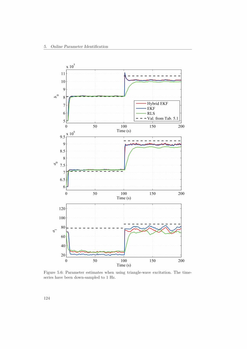
5. Online Parameter Identification
0 50 100 150 2005
6
7
8
9
10
11
x 105
Time (s)
b 0
Hybrid EKFEKFRLSVal. from Tab. 5.1
0 50 100 150 2006
6.5
7
7.5
8
8.5
9
9.5x 10⁶
Time (s)
a 0
0 50 100 150 20020
40
60
80
100
120
Time (s)
a 1
Figure 5.6: Parameter estimates when using triangle-wave excitation. The time-series have been down-sampled to 1 Hz.
124

5.6. Discussion
0 50 100 150 2005
6
7
8
9
10
11
x 105
Time (s)
b 0
Hybrid EKFEKFRLSVal. from Tab. 5.1
0 50 100 150 2006
6.5
7
7.5
8
8.5
9
9.5x 10⁶
Time (s)
a 0
0 50 100 150 20020
40
60
80
100
120
Time (s)
a 1
Figure 5.7: Parameter estimates when using PRBS excitation. The time-series havebeen down-sampled to 1 Hz.
125

5. Online Parameter Identification
For the EKFs, it was observed that different spectral density settings would leadto different, but small, biases in the parameter estimates. Some settings would alsolead to very poor transient behavior, with very large excursions and slow conver-gence. For some settings, the parameter estimates would diverge and asymptoticallyapproach steady-state values far from the values obtained using RLS and frequencyresponse data; this is in accordance with the results in [143]. Thus, global conver-gence to one unique solution is not guaranteed when using EKF for parameteridentification on this system.
When using PRBS excitation, the variance in the parameter estimates fromthe EKFs was rather large. Reducing the process noise spectral densities improvedthis, but reducing them too much led to divergence; the amount of reduction inparameter estimate variance was therefore limited. The RLS method had a muchmore consistent behavior with regards to parameter estimate variance, as well astransient behavior, when using different excitations.
The EKFs provide a convenient method to trade off between rate of conver-gence and the variance in the parameter estimates, by tuning the process noisespectral densities. Tuning the forgetting factor in the RLS method did not provideas dramatic effects on convergence rate, and it consistently seemed rather slowwith regards to convergence rate. Using a non-normalized regressor increased theparameter convergence rate for RLS, but at the expense of larger transients andweaker properties for the signals in the estimation scheme.
As can be seen from Figs. 5.6 and 5.7, there are noticeable biases in the pa-rameter estimates for each parameter identification scheme, and the biases alsoappear to depend on the excitation signal. Some bias can be attributed to theconfiguration of the pre-filter, Wp(s), as well as the tuning of the process noisespectral densities. There is likely some influence from the hysteresis effect in thepiezoelectric actuator, though most of this effect should have been removed by thehigh-pass filter.
The parameter estimates found using each of the EKFs are very similar, butmost noticeably they differ in the obtained value for a0. This difference did not seemto depend on spectral density tuning. The slightly different transient behavior, onthe other hand, was tuning dependent. It can be conjectured that with more carefultuning, the transient behavior can be made more similar.
The quality of the estimates produced by the RLS method were highly depen-dent on the pre-filter, and different filter configurations led to different biases. TheRLS method produced noticeably different estimates than the EKFs. Tuning theforgetting factor and the initial covariance matrix only influenced the transientbehavior and the variance of the parameter estimates. The mean values obtainedasymptotically were the same.
5.7 Conclusions
The RLS method, the continuous EKF, and the hybrid EKF all performed well forparameter identification on this system, when applying a pre-filter to the signalsused. The RLS method was particularly sensitive to the configuration of the pre-filter. The RLS method provided slower convergence than the extended Kalman
126

5.7. Conclusions
filters, but it performed in a more consistent manner with regards to the input sig-nal. The extended Kalman filters needed careful tuning to yield good performanceand to avoid divergence. It was found that the continuous EKF provided the overallbest performance, yielding parameter values that produced the least discrepancybetween model response and measured response.
127


Chapter 6
Robust Adaptive Control
6.1 Introduction
As the dynamic response of typical nanopositioning devices has a fair amount ofuncertainty, both inherently and due to the specific application, the control lawsused also need to have sufficient robustness. This was taken into account for thedamping and tracking control laws in Chapter 3 and the repetitive control schemein Chapter 4.
Although the dynamic response is uncertain, it is dominantly linear and canbe well described for specific operating points. As was demonstrated in Chapter 5,it is possible to obtain good parameter estimates for a linear mass-spring-dampermodel applied to a nanopositioning device operated in open-loop. Nanopositioningdevices should therefore be amenable to model based adaptive control, which inprinciple can provide higher and more consistent performance than standard robuststatic control schemes.
Much of the work pertaining to learning or adaptive type of control for nanopo-sitioning has been done for periodic reference and disturbance signals, in the formof iterative learning control, as discussed in Sections 1.3 and 4.1. The repetitivecontrol scheme discussed in Chapter 4 is also asymptotically invariant to plantuncertainty.
For reference trajectory tracking and disturbance rejection of arbitrary signals,however, the signal repetitiveness can not be exploited. Non-repetitive signals canfor example occur in manipulation and fabrication tasks based on user interaction,and for vertical topography tracking on irregular sample surfaces.
For adaptive control of linear systems, the model reference adaptive control(MRAC) framework [111] is arguably the most exhaustively researched. As such,it is interesting to assess the performance of MRAC applied to a nanopositioningdevice. The main goal in this Chapter is to implement a standard MRAC scheme,and to make the minimum amount of changes to the standard scheme in order forit to work as intended.
129

6. Robust Adaptive Control
6.1.1 Contributions
The standard indirect model reference adaptive control (MRAC) framework is ap-plied in this Chapter in order to develop a complete adaptive control scheme fora nanopositioning device of common design. The MRAC implementation used inthis Chapter is a straight forward extension to the model reference control (MRC)design presented in Section 3.4.7. Extension comes in the form of the implemen-tation of a suitable adaptive law, and the specifics of the implementation of thecontrol law in order to accommodate for time varying parameters.
As was demonstrated in Chapter 5, there are some important considerationsto be made with regards to how to obtain parameter convergence for the adaptivelaw. The most important observation was that a special pre-filter needed in orderto obtain parameter convergence. When operating in closed-loop, the choice ofpre-filter must be further refined.
A similar type of experiment as in Chapter 5 is conducted, where the pay-load mass is changed while operating the nanopositioning device. This experimentprovides a good indication of the ability the adaptive law has to track changes inmodel parameters. The resulting control scheme is believed to be a well performingMRAC scheme, although the comparison would be the standard textbook imple-mentation, which does not work at all. The experimental results should thereforebe indicative of the performance that can be expected applying MRAC to thisparticular type of systems.
6.1.2 Outline
The Chapter is organized as follows. In Section 6.2 the system model used inChapter 5 is reviewed. This forms the basis for the adaptive law. The system modelas used in Section 3.4.7 and Chapter 4 is also discussed, as it forms the basis forthe control law. Some background and discussion on the model reference adaptivecontrol (MRAC) scheme is presented in Section 6.3. Specific design choices for thecontrol law and the adaptive law are discussed in Section 6.4. Finally, experimentalresults for the specific implementation of the MRAC scheme are presented anddiscussed in Section 6.5.
6.2 System Description & Modeling
The experimental system used in this Chapter is almost identical to the systemused in Chapter 5. This is a fairly typical device configuration in systems used formotion control in general. As described in Section 5.2, it consists of the positioningmechanism shown in Fig. 2.3, as well as additional necessary instrumentation,including anti-aliasing and reconstruction filters, a voltage amplifier, a capacitivedisplacement sensor, and a standard hardware-in-the-loop (HIL) system.
As was the case for the model reference control (MRC) scheme in Section 3.4.7,a plant model which includes the dynamics for the nanopositioning stage, as wellas the dynamics of the anti-aliasing and reconstruction filters, is used. A morecomplete model would also include the amplifier and sensor dynamics, and thetime-delay incurred by the zero-order-hold (ZOH) elements in the digital-to-analog
130

6.2. System Description & Modeling
Table 6.1: Identified parameters for the model (6.1), using frequency response data.
Parameter Value Unit Parameter Value Unit1) With payload on sample platform
b0 1.97·106 μm/s2V b0/a0 0.109 μm/Va0 18.1·106 1/s2 f0 677 Hza1 127 1/s ζ 0.0149
2) Without payload on sample platformb0 2.33·106 μm/s2V b0/a0 0.107 μm/Va0 21.9·106 1/s2 f0 744 Hza1 131 1/s ζ 0.0140
converter (DAC) and analog-to-digital converter (ADC). The attainable samplingrate is fast enough for the phase-lag due to the ZOH elements to be insignificantwithin the bandwidth of the control law, and the amplifier and sensor dynamics isfaster than what is possible to represent with a discretized model when using theattainable sampling rate. A higher order model results in a control law of higherorder, which also reduces the attainable sampling rate. The main reason for usingthe highest possible sampling rate is that the noise floor due to the DAC and ADC,given a fixed quantization unit, can only be reduced by increasing the samplingrate, cf. Section 4.5.1. The sampling rate also determines the accuracy and stabilityof the numerical integration scheme [62].
This plant model is the model which has the highest practically obtainableaccuracy for this system. A diagram of the plant model is found in Fig. 3.3.
6.2.1 Mechanical Model
The mechanical model used is as presented in Section 5.2.1, and is also equivalentto the model used in Section 3.4.7. Denoting the deflection w (m), the transfer-function from applied voltage ua (V) to the displacement for the nanopositioningstage is
Gw(s) =w
ua(s) =
β0
s2 + 2ζω0s + ω02 =b0
s2 + a1s + a0, (6.1)
noting that β0 = b0 and ω0 = 2πf0.The frequency response is recorded for the x-axis (the y-axis was used in Chap-
ter 5), using bandwidth-limited white noise excitation. As was the case in Chap-ter 5, the system is operated in two different payload configurations. The pay-load mass is approximately 15.7 g. The responses are displayed in Fig. 6.1. Themodel (6.1) is fitted to the frequency response data using the MATLAB SystemIdentification Toolbox, and the resulting parameter values are presented in Tab. 6.1.The response of the model (6.1) using these parameters is also displayed in Fig. 6.1for comparison.
131

6. Robust Adaptive Control
Mag
nitu
de (d
B)
Phas
e (d
eg)
Frequency (Hz)
Measured response w/payloadModel fitMeasured response wo/payloadModel fit
Figure 6.1: Measured frequency response and model response, for the two payloadconfigurations, and corresponding model fits.
6.2.2 Anti-Aliasing & Reconstruction Filters
The anti-aliasing and reconstruction filters, Wa(s) and Wr(s) respectively, aresecond-order Butterworth filters, and are chosen to be identical, Wr(s) = Wa(s),for convenience. They have a transfer-function of the form
Wa(s) = Wr(s) =ωc
2
s2 +√2ωcs + ωc
2, (6.2)
where ωc is the cut-off frequency. As the cut-off frequency ωc for the anti-aliasingand reconstruction filters used in the experimental set-up is user programmable,the filters provide an extra degree of freedom for the control law tuning. As notedin Section 3.4.7, the filters can be used to attenuate non-modeled high-frequencydynamics, as well as to attenuate quantization and sensor noise, given that thecut-off frequency ωc is below the Nyquist frequency. The cut-off frequency selection
132

6.2. System Description & Modeling
can also to some degree improve the nominal closed-loop sensitivity response androbustness properties.
6.2.3 Complete Plant Model
The complete model for the system presented in Fig. 3.3 is
ym
u(s) = Wa(s)Gw(s)Wr(s) .
The usage of this model for the design of the MRAC scheme will not provide goodperformance with respect to the closed-loop sensitivity function, as it will haveconstant gain at low frequencies. Due to external disturbances, introduced by thehysteresis and creep non-linearities, and in order to reduce the impact of model un-certainty, it is advisable to add integral action to the control law [157]. The responseof the closed-loop sensitivity function at lower frequencies will then improve. Thiscan be done by augmenting the system with an integrator, implemented as partof the control scheme. The plant model, with regards to the synthesis equations inAppendix E, used is thus
Gp(s) =1s
Gw(s)Wr(s)Wa(s) , (6.3)
which is the same structure as for (3.50). The overall model order is np = 7.
6.2.4 Model Uncertainty
The uncertainty in the nanopositioner dynamics is due to specific user applications,as well as inherent properties in the actuator and mechanical structure.
Users will typically need to position payloads of various masses, and thereforethe resonance frequencies and the effective control gain of the mechanical structurewill change every time a new payload is attached [140]. This is clearly demonstratedby inspecting the frequency responses for the two payload configurations in Fig. 6.1,and the corresponding parameter values for the model (6.1) in Tab. 6.1.
As can be seen from Fig. 6.1, the response of the first vibration mode is wellapproximated by the second-order model (6.1) using the identified parameters inTab. 6.1, for both payload configurations. It is evident that there exist higher ordermodes in the system, and the second and third vibration modes are clearly visiblein Fig. 6.1. These higher order modes have relatively small magnitude responses incomparison to the first, and they have shapes and directions that will make themdifficult to control using the mounted actuator; thus the only practical solution isto avoid exiting these modes by limiting the bandwidth of the control law.
As discussed in Section 1.2.1 and Chapter 2, another second source of uncer-tainty is due to the piezoelectric actuator, which has inherent variations in theeffective control gain due to changes in actuator temperature, offset voltage, dis-placement range, as well as due to depolarization of the piezoelectric actuator. Thehysteresis and creep non-linearities present in all piezoelectric actuators are themain contributors to the change in effective gain, and this is directly dependent
133
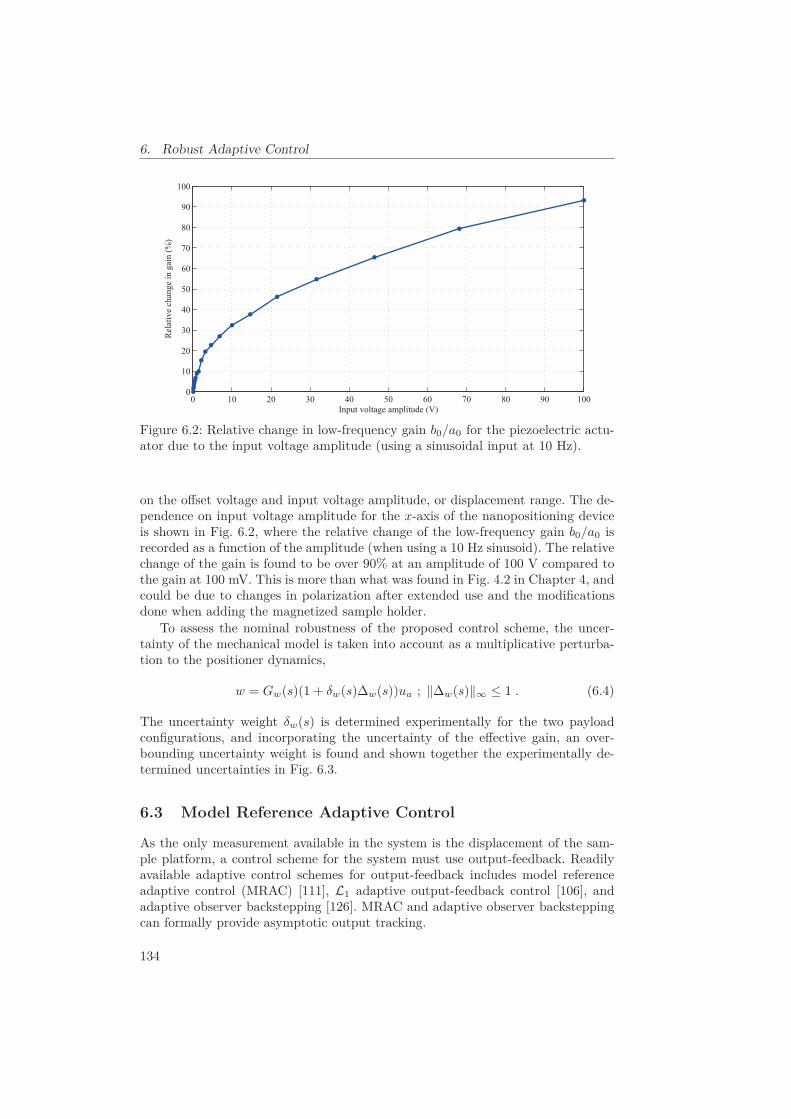
6. Robust Adaptive Control
0 10 20 30 40 50 60 70 80 90 1000
10
20
30
40
50
60
70
80
90
100
Input voltage amplitude (V)
Rel
ativ
e ch
ange
in g
ain
(%)
Figure 6.2: Relative change in low-frequency gain b0/a0 for the piezoelectric actu-ator due to the input voltage amplitude (using a sinusoidal input at 10 Hz).
on the offset voltage and input voltage amplitude, or displacement range. The de-pendence on input voltage amplitude for the x-axis of the nanopositioning deviceis shown in Fig. 6.2, where the relative change of the low-frequency gain b0/a0 isrecorded as a function of the amplitude (when using a 10 Hz sinusoid). The relativechange of the gain is found to be over 90% at an amplitude of 100 V compared tothe gain at 100 mV. This is more than what was found in Fig. 4.2 in Chapter 4, andcould be due to changes in polarization after extended use and the modificationsdone when adding the magnetized sample holder.
To assess the nominal robustness of the proposed control scheme, the uncer-tainty of the mechanical model is taken into account as a multiplicative perturba-tion to the positioner dynamics,
w = Gw(s)(1 + δw(s)Δw(s))ua ; ‖Δw(s)‖∞ ≤ 1 . (6.4)
The uncertainty weight δw(s) is determined experimentally for the two payloadconfigurations, and incorporating the uncertainty of the effective gain, an over-bounding uncertainty weight is found and shown together the experimentally de-termined uncertainties in Fig. 6.3.
6.3 Model Reference Adaptive Control
As the only measurement available in the system is the displacement of the sam-ple platform, a control scheme for the system must use output-feedback. Readilyavailable adaptive control schemes for output-feedback includes model referenceadaptive control (MRAC) [111], L1 adaptive output-feedback control [106], andadaptive observer backstepping [126]. MRAC and adaptive observer backsteppingcan formally provide asymptotic output tracking.
134

6.3. Model Reference Adaptive Control
102 103
0
10
20
30M
agni
tude
(dB
)
Frequency (Hz)
Uncertainty (w/payload)Uncertainty (wo/payload)Overbound
Figure 6.3: Open-loop uncertainty weight δw(s), for the two payload configurationsand an over-bounding approximation.
L1 adaptive output-feedback control provides an disturbance observer adapt-ing to the discrepancy between the plant output and a reference model, and thestability and performance will depend on the choice of reference model and a low-pass filter which is non-trivial to find in general. For a first-order reference model,however, it is fairly straight forward to find these filters. The control scheme willin that case be equivalent to a proportional-integral (PI) control law [106], and thetuning procedure for the modified PI control law used in Chapter 4 also providegood performance for the first-order reference model L1 adaptive control scheme.
Adaptive observer backstepping is dependent on non-linear damping terms,which can lead to impractically large actuation forces, and also produces verycomplicated control laws. The MRAC scheme was deemed to be the most feasiblechoice. The control law and adaptive law is decoupled, such that the control lawand adaptive law can be designed separately. The design procedures for the controllaw and adaptive law are also fairly straight forward.
6.3.1 Control Scheme Description
Model reference adaptive control (MRAC), and the static variety, model refer-ence control (MRC) is described in Appendix E. As described in Appendix E, theMRAC scheme consists of a control law and an adaptive law, that can be designedindependently and then combined using the certainty equivalence principle [111].An MRAC scheme can generally be implemented in direct and indirect form. Themain difference is that for the direct form, the control law parameters are esti-mated directly, whereas for the indirect form, the plant parameters are estimatedand subsequently mapped to the control law parameters.
The chosen plant model order is np = 7, which for the direct case requires2np = 14 parameters to be estimated. As only three plant parameters, b0, a1, anda0, are uncertain and require estimation, employing an indirect MRAC reduces
135

6. Robust Adaptive Control
the complexity and computational requirements of the parameter identificationsignificantly. In addition, experience suggests that parameter convergence is muchmore difficult to achieve with a larger number of estimated parameters.
The indirect MRAC scheme requires the application of a normalized adaptivelaw, which is necessary for the stability properties of the indirect MRAC scheme,according to Theorem 6.6.2 in [111]. Normalization ensures boundedness of themeasured signals used in the adaptive law.
Applicable (normalized) adaptive laws include the gradient method based oneither instantaneous or integral cost functions, and the least-squares method. The(normalized) recursive least-squares method was used in Chapter 5, together withthe extended Kalman filter. For the extended Kalman filter there does not existany general proofs of convergence, and the estimates are not guaranteed to bebounded. Stability can therefore not be established theoretically when using theextended Kalman filter for parameter estimation.
All four of the above mentioned methods were implemented and applied to-gether with the MRAC control law, and for the system at hand all four methodsprovided reasonable parameter convergence, given that the signals used were care-fully pre-filtered. The gradient method based on the integral cost function (integraladaptive law) behaves similarly to the least-squares method, but with the addedbenefit of user selectable convergence rate. The method also provides theoreticalstability results for the overall scheme, and was therefore chosen to be used in theimplemented MRAC scheme. The integral adaptive law is described in Section D.2.
6.4 Design Choices
6.4.1 Control Law
In this Section, the control law design from Section 3.4.7 is reviewed. Assuminggood knowledge of the plant model Gp(s), there are two main design choices withregards to the control law, which is the choice of the reference model Wm(s) andthe output filter 1/Λ(s). The main limiting factor in determining these filters, is theuncertainty of the plant model, which for the system at hand is due to non-modeledhigh-frequency dynamics. As described in Section E.2, the nominal control law canalso be expressed in terms of the feed-forward filter
C(s) =c0Λ(s)
Λ(s) − θ1Tα(s)
and feedback filter
F (s) = −θ2Tα(s) + θ3Λ(s)
c0Λ(s),
i.e., the control law can be written as
up = C(s)(r − F (s)yp) .
The complementary sensitivity function for a set of nominal plant parameter esti-mates can then be found as
T (s) =C(s)Gp(s)
1 + C(s)F (s)Gp(s).
136

6.4. Design Choices
Since T (s) = Wm(s), the stability criterion
‖F (s)Wm(s)δw(s)‖∞ < 1 (6.5)
can be used to choose Wm(s) and 1/Λ(s) to obtain robustness against uncertaindynamics.
For simplicity, the reference model Wm(s) was chosen to be a seventh orderButterworth filter with cut-off frequency ωm, i.e.qm = 0 and pm = 7, and sincethe plant model Gp(s) does not have any zeros, the polynomial Λ(s) should be ofdegree np − 1 = 6, and the zeros of Λ(s) was chosen to have a Butterworth patternwith radius ωl.
The plant model includes the reconstruction and anti-aliasing filters, Wr(s) andWa(s), both having the user-programmable cut-off frequency ωc. As already noted,the filters can be used to attenuate non-modeled high-frequency dynamics, as wellas to attenuate quantization and sensor noise, given that the cut-off frequencyωc is below the Nyquist frequency. The cut-off frequency selection can also tosome degree improve the nominal closed-loop sensitivity response and robustnessproperties.
The nominal tuning of the control law depends on the choice of ωm, ωl, and ωc.As the plant is open-loop stable, and since it is augmented with an integral state,the performance in terms of the sensitivity function
S(s) =1
1 + C(s)F (s)Gp(s)
of the nominal closed-loop system is in general improved by choosing a bandwidthas high as possible for the reference model Wm(s) and the output filter 1/Λ(s),i.e., choosing ωm and ωl as large as possible.
The choice of ωc is not as straight forward, as there can be found an optimalvalue which minimizes ‖S(s)‖∞. By a course exhaustive grid search over ωm, ωl,and ωc, evaluating (6.5) when using the nominal parameters for the two payloadconfigurations from Tab. 6.1, an approximate optimal value for ωc, and the ap-proximate highest bandwidth for Wm(s) and 1/Λ(s) without violating (6.5) wasselected, and the result is shown in Tab. 6.2. The nominal frequency responses ofthe complementary sensitivity function, T (s), the transfer-function (3.10) from rto ε, E(s), the transfer-function (3.12) from du to w, and the sensitivity functionS(s) using the parameters in case 1) in Tab. 6.1 are shown in Fig. 6.4. As can beseen, the expected bandwidth is approximately 150 Hz.
The evaluation of the robust stability criterion (6.5) is shown is Fig. 6.6, forthe over-bounding uncertainty weight in Fig. 6.3.
The control law is implemented as shown in Fig. 6.5. With reference to the aug-mented plant model (6.3), the filters Wr(s), Wa(s) and the nanopositioning device,modeled as Gw(s), are physical components, whereas the integrator is implementedin software. The control law (E.1) is therefore modified to be
up =1s
(θ1
T α(s)Λ(s)
up + θ2T α(s)Λ(s)
yp + θ3yp + c0r
).
137
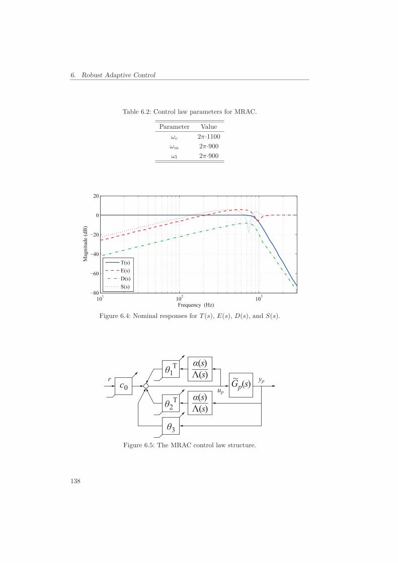
6. Robust Adaptive Control
Table 6.2: Control law parameters for MRAC.
Parameter Valueωc 2π·1100ωm 2π·900ωl 2π·900
101 102 103
0
20
Mag
nitu
de (d
B)
Frequency (Hz)
T(s)E(s)D(s)S(s)
Figure 6.4: Nominal responses for T (s), E(s), D(s), and S(s).
3
(s)(s)
(s)(s)
1T
c0 Gp(s)
2T
up
ypr ~
Figure 6.5: The MRAC control law structure.
138
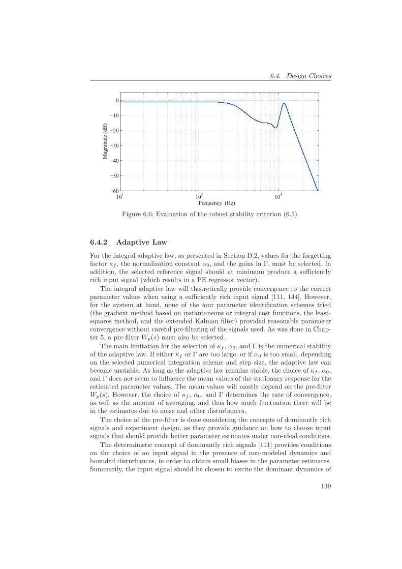
6.4. Design Choices
101 102 103
0M
agni
tude
(dB
)
Frequency (Hz)
Figure 6.6: Evaluation of the robust stability criterion (6.5).
6.4.2 Adaptive Law
For the integral adaptive law, as presented in Section D.2, values for the forgettingfactor κf , the normalization constant α0, and the gains in Γ, must be selected. Inaddition, the selected reference signal should at minimum produce a sufficientlyrich input signal (which results in a PE regressor vector).
The integral adaptive law will theoretically provide convergence to the correctparameter values when using a sufficiently rich input signal [111, 144]. However,for the system at hand, none of the four parameter identification schemes tried(the gradient method based on instantaneous or integral cost functions, the least-squares method, and the extended Kalman filter) provided reasonable parameterconvergence without careful pre-filtering of the signals used. As was done in Chap-ter 5, a pre-filter Wp(s) must also be selected.
The main limitation for the selection of κf , α0, and Γ is the numerical stabilityof the adaptive law. If either κf or Γ are too large, or if α0 is too small, dependingon the selected numerical integration scheme and step size, the adaptive law canbecome unstable. As long as the adaptive law remains stable, the choice of κf , α0,and Γ does not seem to influence the mean values of the stationary response for theestimated parameter values. The mean values will mostly depend on the pre-filterWp(s). However, the choice of κf , α0, and Γ determines the rate of convergence,as well as the amount of averaging, and thus how much fluctuation there will bein the estimates due to noise and other disturbances.
The choice of the pre-filter is done considering the concepts of dominantly richsignals and experiment design, as they provide guidance on how to choose inputsignals that should provide better parameter estimates under non-ideal conditions.
The deterministic concept of dominantly rich signals [111] provides conditionson the choice of an input signal in the presence of non-modeled dynamics andbounded disturbances, in order to obtain small biases in the parameter estimates.Summarily, the input signal should be chosen to excite the dominant dynamics of
139

6. Robust Adaptive Control
the system to a level that dominates the disturbances, and have a spectral contentthat avoids excitation of non-modeled dynamics.
Somewhat similarly, the stochastic concept of experiment design [93, 182], pro-vides methods to construct input signals of finite power that will maximize con-ditions on the Fisher information matrix, which should then provide parameterestimates with minimal variance when using measurements corrupted by colorednoise. The Fisher information matrix in the frequency domain involves the pa-rameter sensitivity functions for the plant model. A finite energy signal will thentypically be optimal for some condition on the information matrix if the spec-tral content is concentrated in frequency domains where the parameter sensitivityfunctions of a model have peaks. An optimal input signal in this sense should alsoimprove the convergence rate of the parameter estimates [150].
As designing an optimal input signal is usually not feasible for arbitrary track-ing control tasks, a practically feasible solution is to find a pre-filter which empha-sizes certain frequency domains in the signals used in the parameter identificationscheme [144, 157], as discussed in Chapter 5. In addition to provide more optimalsignals with regards to the information matrix, the pre-filter is also beneficial sinceit can attenuate disturbances and non-modeled effects; thus a more dominantlyrich signal.
A heuristic approach is chosen in order to select a reasonable pre-filter Wp(s).As prior knowledge of approximate parameter values is available from frequency re-sponse data, a nominal model reference control law (MRC) is found. Data collectedfrom the plant while running in closed-loop using the MRC then provide a reason-able approximation to the expected input signal and noise correlation when usingthe MRAC. Using these data off-line, different filter choices are tested, accordingto the following considerations.
As was demonstrated in Chapter 5, the parameter sensitivities of a mass-spring-damper system suggest an emphasis on a frequency domain around the expectedresonance frequencies of the system, a bandpass filter. As the scheme requiresdifferentiation of the measured deflection, the bandpass filter must have a relativedegree equal to the highest order of differentiation needed, so that the filters willbe proper. To provide some low-pass filtering, the relative degree should be higher.
Choosing only a bandpass filter W1(s) with a narrow passband around expecteddominant resonant frequencies results in poor low-frequency gain estimation for thissystem, i.e., the ratio b0/a0 is too low. Adding another bandpass filter in parallel,with a narrow passband around the fundamental frequency of the reference signaland a selectable gain k2W2(s), increases the parameter identification accuracy. Thegain k2 can not be too large, as it will impact the accuracy of parameters dependingon the natural frequency and damping coefficient, a1 and a0. The filter that is usedis thus
Wp(s) = W1(s) + k2W2(s) , (6.6)
where the cut-off frequencies for W1(s) is [f l1, fh
1 ] = [475, 900] and for W2(s) is[f l
2, fh2 ] = [fr − 10, fr + 10], fr being the fundamental frequency of the reference
signal. The filter gain was chosen to be k2 = 0.01. The chosen pre-filter is shownin Fig. 6.7.
140
6.5. Experimental Results & Discussion
For the model (6.1), assuming a displacement measurement w, the parametervector θ in the parametric model (D.1) is here denoted θp as given as
θp = [b0, a1, a0]T .
The regressor vector is then found as
ϕ = [ua, −w, −w]T ,
and the output of the model is z = w. To account for the known dynamics in thereconstruction and anti-aliasing filters, determined by the cut-off frequency ωc, andincorporating the pre-filter, the output z and regressor ϕ is constructed as
z = s2Wp(s)ym
andϕ(s) = [Wr(s)Wa(s)Wp(s)up, −sWp(s)ym, −Wp(s)ym]T ,
as illustrated in Fig. 5.4.Reasonable values for κf , α0, and Γ, trading-off convergence rate and forgetting
rate or averaging, were found as κf = 2, α0 = 0.001, and
Γ = diag([5 · 106, 5 · 101, 5 · 107]) .
The parameter vector θ for the plant model (6.3), Gp, is determined by theconvolution of the polynomials in the numerator and denominator of Wr(s), Wa(s),and Gw(s), as well as the integrator 1/s. The parameter mapping from the adaptivelaw to the control parameters is therefore θp → θ → θc, where
θc =[θ1
T, θ2T, θ3, c0
]T.
6.5 Experimental Results & Discussion
6.5.1 Description of the Experimental System
The experimental set-up consisted of a Dell Optiplex 760 computer equipped witha PCI-6221 data acquisition board from National Instruments, running the xPCTarget real-time operating system for hardware-in-the-loop simulations, a ADE6810 capacitive gauge and ADE 6501 capacitive probe from ADE Technologies, aPiezodrive PDL200 voltage amplifier, the custom-made long-range serial-kinematicnanopositioner (see Fig. 2.3), two SIM 965 programmable filters, and a SIM983 scal-ing amplifier from Stanford Research Systems. With the xPC Target, a maximumsampling frequency of fs = 40 kHz was achieved for the complete MRAC scheme,and used for all the experiments. For numerical integration, a third-order Runge-Kutta scheme (Bogacki-Shampine) [62] was used. In order to achieve a highersampling frequency, the adaptive law and parameter mapping was implementedusing the C programming language.
141

6. Robust Adaptive Control
100 101 102 103 104 105
0
Mag
nitu
de (d
B)
Frequency (Hz)
Figure 6.7: Pre-filter Wp(S).
6.5.2 Experiments
Four experiments are performed to assess the tracking and parameter estimationperformance. A triangular reference signal with a fundamental frequency fr = 50Hz is used, which is sufficiently rich for parameter estimation for this system. Thecontrol bandwidth is approximately 150 Hz, thus using a relatively high funda-mental frequency should help elucidate model discrepancies and disturbances inthe system response. First, the ability to track parameter changes is evaluated byadding a payload of 15.7 g while the system is running. Next, three experimentswere done to find the asymptotic parameter estimates for various configurations,as well as the stationary tracking error.
6.5.3 Results & Discussion
The experimental results are presented in Figs. 6.8 and 6.9, and Tab. 6.3.From Fig. 6.8 it is evident that reasonable parameter convergence is achieved,
and the adaptive law is able to track parameter changes when the payload is addedafter approximately 5 seconds. There are discrepancies in the estimates comparedto the values in Tab. 6.1, especially for the b0 and a1 parameters. The discrepancyfor b0 is mainly due to the larger driving voltage amplitude used in the experiment,compared to the amplitude used to find the frequency response. The discrepancy fora1 is likely due to the presence of colored noise due to feedback and the hysteresisdisturbance, since the parameter sensitivity for the model (6.1) with respect to a1is very small, as was pointed out in Chapter 5. The small oscillations in the a1estimate is due to noise, and can be reduced by decreasing, e.g., the correspondinggain in Γ, at the expense of slower convergence.
By inspection of case 1) and 2) in Tab. 6.3, it can seen that the estimatesfor the natural frequency and the damping ratio is underestimated in case 1), andoverestimated in case 2). This is likely due to the tuning of the pre-filter, as the biaschange, and the accuracy improves, by fine tuning of the pre-filter to the specific
142
6.6. Conclusions & Future Works
Table 6.3: Asymptotic values for the estimates for the parameters in the model (6.1)and stationary tracking errors for the MRAC scheme for various configurations.
1) No payload; 50 Hz, 3 μm amp. triangle-wave ref.b0 2.79·106 μm/s2V b0/a0 0.130 μm/Va0 21.4·106 1/s2 f0 737 Hza1 297 1/s ζ 0.0321RMSE: 0.113 μm RMSE relative: 6.52 %Max. error: 0.213 μm Max. relative error: 7.31 %
2) Payload; 50 Hz, 3 μm amp. triangle-wave ref.b0 2.33·106 μm/s2V b0/a0 0.131 μm/Va0 17.8·106 1/s2 f0 672 Hza1 32.9 1/s ζ 0.00390RMSE: 0.101 μm RMSE relative: 5.82 %Max. error: 0.186 μm Max. relative error: 6.40 %
3) Payload; 50 Hz, 6 μm amp. triangle-wave ref.b0 2.46·106 μm/s2V b0/a0 0.144 μm/Va0 17.1·106 1/s2 f0 657 Hza1 -95.0 1/s ζ -0.0115RMSE: 0.282 μm RMSE relative: 8.15 %Max. error: 0.520 μm Max. relative error: 8.94 %
configuration. Case 2) and 3) demonstrate the ability to track the change in low-frequency gain b0/a0 due to change in displacement range, as should be expectedby the results in Fig. 6.2, but there is also a noticeable change in the estimatednatural frequency and damping ratio, which also depend on the pre-filter tuning.
As already noted in Section 6.4.2, the low-frequency gain is always underesti-mated. This can be seen by looking at Fig. 6.9, where it is apparent that the systemresponse overshoots the reference. This can be confirmed by fixing the parameterestimates and manually increasing the b0 estimate, in which case the error can bereduced.
6.6 Conclusions & Future Works
6.6.1 Conclusions
A working implementation of a MRAC scheme has been demonstrated, and theexperimental results obtained provide an indication of the achievable performancethat can be expected when applied to a flexible smart structure. The main chal-lenge was to achieve reasonable convergence for the parameter estimation scheme,and this was demonstrated to be possible by the use of a special pre-filter. Onemajor limitation with regards to performance is the difficulty in having simulta-
143

6. Robust Adaptive Control
0 1 2 3 4 5 6 7 8 9 10
1
1.5
2
2.5
3
3.5
x 106
Time (s)
b 0
Adaptive law estimateVal. from Tab. 6.1
0 1 2 3 4 5 6 7 8 9 101.6
1.8
2
2.2
2.4
2.6
x 107
Time (s)
a 0
0 1 2 3 4 5 6 7 8 9 10
0
50
100
150
200
250
300
350
400
450
Time (s)
a 1
Figure 6.8: Estimated parameters when adding a payload to the sample platform,using a 50 Hz triangle-wave reference signal with 3 μm amplitude. The time-serieshave been down-sampled to 40 Hz.
144

6.6. Conclusions & Future Works
9.97 9.975 9.98 9.985 9.99 9.995 10
0
1
Time (s)
Dis
plac
emen
t (μm
)
MeasurementModelError
Figure 6.9: Stationary response, with payload on the sample platform, using a50 Hz triangle-wave reference signal with 3 μm amplitude.
neous accurate estimation of the parameters determining the low-frequency gainand the parameters dependent on the damping ratio and natural frequency of thesystem. This is most likely due to the presence colored noise due to feedback andthe hysteresis and creep nonlinearities, which also causes bounded disturbances,and necessitates integral action in the control law. The suppression of these distur-bances are dependent on the achievable control law bandwidth, which main limitingfactor is the presence of non-modeled and practically uncontrollable higher-ordervibration modes.
6.6.2 Future Works
The parameter estimation is very sensitive to the choice of pre-filter Wp(s), the ac-tual plant parameters, the chosen control law parameters, and reference signal. Toimprove on the parameter estimation performance, it might be possible to find bet-ter choices for Wp(s), and the application of more elaborate identification schemes,specifically tailored for closed-loop identification such as the recursive instrumentalvariable method [88], should be investigated.
In order to make the control scheme more robust in general, well known tech-niques such as parameter projection and adaptation dead-zones should be used toavoid large parameter drift. Since integral action is added to the control law, asuitable anti-windup scheme should also be added.
Some performance improvement for the MRAC scheme presented can possiblybe achieved by a better nominal tuning of the control law, which is determinedby the choice of reference model Wm(s), anti-aliasing and reconstruction filtersWr(s), Wa(s), and output filter 1/Λ(s).
145


Appendices
147


Appendix A
Piezoelectric Transducers
This Appendix is a summary of the standard theory on piezoelectric transducers.It is collated from material found in [1, 2, 7, 23–25, 38, 54, 55, 62, 112, 115, 134,162, 164, 171–173]. Some details are added to clarify the usage of the theory.
A.1 Piezoelectricity
Piezoelectricity is the ability of some materials to generate an electric charge inresponse to applied mechanical stress. If the material is not short-circuited, thegenerated charge induces a voltage across the material that can be measured by avoltmeter. The piezoelectric effect is reversible, and an applied electric field gen-erates strain in the material, resulting in a change in geometry, which can bemeasured by a pair of calipers. The production of charge when a stress is applied iscalled the direct piezoelectric effect, and the production of strain when an electricfield is applied is called the converse piezoelectric effect.
The direct effect is illustrated in Fig. A.1, which shows a cylinder of piezoelec-tric material under a no-load condition, and subjected to a tensile stress and acompressive stress. The generated charge is due to a change in dipole moment, andappears as a voltage that can be measured, analogous to a voltage appearing onthe terminals of a capacitor that has been charged.
polin
g ax
is
f f
Figure A.1: Illustration of the direct piezoelectric effect.
149

A. Piezoelectric Transducerspo
ling
axis
Figure A.2: Illustration of the converse piezoelectric effect.
The converse effect is illustrated in Fig. A.2, which shows a cylinder of piezo-electric material when applying an electric field with polarity in the same directionas the poling axis, which produces a positive strain (lengthening) along the polingaxis, and when applying an electric field with polarity in the opposite directionof the poling axis, which produces a negative strain (shortening) along the polingaxis.
The direct piezoelectric effect was discovered in 1880 by the Pierre and JacquesCurie during experiments on crystals of tourmaline, quartz, topaz, cane sugar,and Rochelle salt. The existence of the converse piezoelectric effect was predictedby Gabriel Lippmann in 1881 and the existence was experimentally confirmed byPierre and Jacques Curie. The 20 natural crystal classes capable of piezoelectricity,and the physical properties involved, were rigorously defined using tensor analysisby Woldemar Voigt in 1910. The first step toward an engineering application wastaken in 1916 by Paul Langevin, who constructed an underwater ultrasonic sourceconsisting of a piezoelectric quartz element sandwiched between steel plates, whichwas one of the first sonar devices, used for submarine detection.
The piezoelectric effect is anisotropic, and can only be found in materials whosecrystal structure has no center of symmetry. In addition to naturally occurringmaterials, some modern synthetic materials exhibit piezoelectricity. These includelead zirconate titanate, a ceramic, and polyvinylidene fluoride, a polymer, whichare commonly used in transducers, as they have high piezoelectric constants.
Most materials used for transducers are ferroelectric, and for these materialspiezoelectricity always occur below a certain temperature called the Curie tem-perature. The most common example of a ferroelectric is lead zirconate titanate(PZT), which has the chemical formula Pb[ZrxTi1−x]O3, x ∈ [0, 1]. The materialcan be considered to be a mass of minute crystallites. These crystallites have dif-ferent properties above and below the Curie temperature, and an elementary cellof PZT material is illustrated in Fig. A.3, for these two states.
Above the Curie temperature, the structure is centrosymmetric with negativeand positive charge sites coinciding, so there are no dipoles present in the material,and it is said to be paraelectric. Below the Curie temperature, the elementary cellhas a built-in electric dipole, due to a tetragonal symmetry, where the negative andpositive charge sites do no longer coincide. The dipoles are aligned in regions calledWeiss domains, generating a net dipole moment for a domain, but the domainsthroughout the material are randomly oriented, and the net macroscopic effectis therefore zero for the whole material. The dipoles can be aligned, however, in
150

A.1. Piezoelectricity
O2- Pb2+ Ti4+, Zr4+
+
–
Figure A.3: Lead zirconate titanate (Pb[ZrxTi1-x]O3) (PZT) elementary cell, abovethe Curie temperature (left) and below (right).
–
+
–
+
–
+
–
+–
+
–
+
–
+
–
+–
+
–
+
–
+
–
+
–
+
–
+
–
+
–
+–
+
–
+
–
+
–
+–
+
–
+
–
+
–
+–
+
–
+
– +
–
+–
+–
+ –
+
–
+
–
+–
+
–
+
–
+
+
–
polin
g ax
is
polin
g vo
ltage
Figure A.4: Electric dipole moments in Weiss domains, before (left), during (mid-dle), and after (right) polarization.
a process called poling. If the material is poled, some Weiss domains are grownat the expense of others, such that the net dipole moment can be noticed on amacroscopic scale.
The poling process involves heating the material above the Curie temperatureand subsequently cooling the material in the presence of a high electric field. Theelectric field aligns the dipoles, and the dipoles become fixed below the Curie tem-perature, thus making the material permanently piezoelectric. This is illustrated inFig. A.4. The property is lost if the material is reheated above the Curie tempera-ture, if an excessive electric field is applied in the direction opposed to the polingdirection, or due to excessive vibrations. The dipoles also naturally tend to changealignment over time, a process known as aging.
The word piezoelectricity means “electricity by pressure”, and is derived fromthe Greek piezein, which means to push.
151

A. Piezoelectric Transducers
D
E
e
-e
permittivity [2]
electric displacement (1)
electric field intensity (1)
strain (2)
stress (2)
elasticity [4]
direct piezoelectric effect [3]converse piezoelectric effect [3]
sc
d d
Figure A.5: Electromechanical relations in crystals (piezoelectricity). Tensor ranksof the variables are shown in parentheses, and tensor ranks of the properties areshown in square brackets.
A.1.1 Piezoelectric Constitutive Equations
Materials exhibiting piezoelectric effects can also exhibit electrothermal effects (py-roelectricity) and thermoelastic effects, but this will not be considered here. Thetensor relationships describing piezoelectric effects are presented diagrammaticallyin Fig. A.5. The tensor description here gives multilinear relationships between vari-ables through constant properties, and is considered to be a small-signal model. Itwill therefore not explain the non-linear effects observed in piezolectric transducers,such as hysteresis and creep. The tensor relationships are given in matrix form.
Piezoelectric constitutive equations can be found on several different forms,which are equivalent. The properties used are measured under different conditions,but properties found using one set of conditions can be transformed to another setof conditions using certain relationships.
Four equivalent forms of the constitutive equations
The strain-charge form of the constitutive equations are given as
ε = sEσ + dTE (A.1)D = dσ + κσE , (A.2)
the stress-charge form as
σ = cEε − eTE (A.3)D = eε + κεE , (A.4)
the strain-voltage form as
ε = sDσ + gTD (A.5)E = −gσ + βσD , (A.6)
152

A.1. Piezoelectricity
and the stress-voltage form as
σ = cDε − hTD (A.7)E = −hε + βεD . (A.8)
The symbols used for for the variables are:ε strain (m/m), second order tensorσ stress (N/m2), second order tensorE electric field (V/m), first order tensorD electric displacement (C/m2), first order tensor
The symbols used for for the properties are:s elastic compliance (m2/N), fourth order tensorc elastic stiffness (N/m2), fourth order tensore piezoelectric strain-charge modulus (C/m2), third order tensord piezoelectric stress-charge modulus (m/V) = (C/N), third order tensorg piezoelectric stress-voltage modulus ((V m)/N) = (m2/C), third order tensorh piezoelectric strain-voltage modulus (V/m) = (N/C), third order tensorκ permittivity (dielectric constant) (F/m) = (C/(V m)), second order tensorβ impermittivity (m/F), second order tensor
The measurement conditions used when finding a property is indicated by a su-perscript. A property found under a constant electric field is denoted ()E . In thiscase the electrodes are short circuited (closed circuit). Conversely, a property mea-sured under a constant electric displacement is denoted ()D, and this means thatthe electrodes are not connected (open circuit). A property found under constantstress is denoted ()σ. The material is then free to expand, and is not mechanicallyconstrained in any way. The converse situation is when a property is found underconstant strain, which is denoted ()ε. In this case, the material is clamped, whichmeans that it is mechanically constrained and unable to expand in any direction.()E closed circuit condition()D open circuit condition()σ constant stress (free) condition()ε constant strain (clamped) condition
Example A.1:Referring to the illustration in Fig. A.1, the generated charge is due to
D = dσ ,
and there is no applied electric field, only applied stress. Similarly, referring toFig. A.2, the generated strain is due to
ε = dTE
when applying an electric field, and there is no stress due to the absence of me-chanical constraints.
153
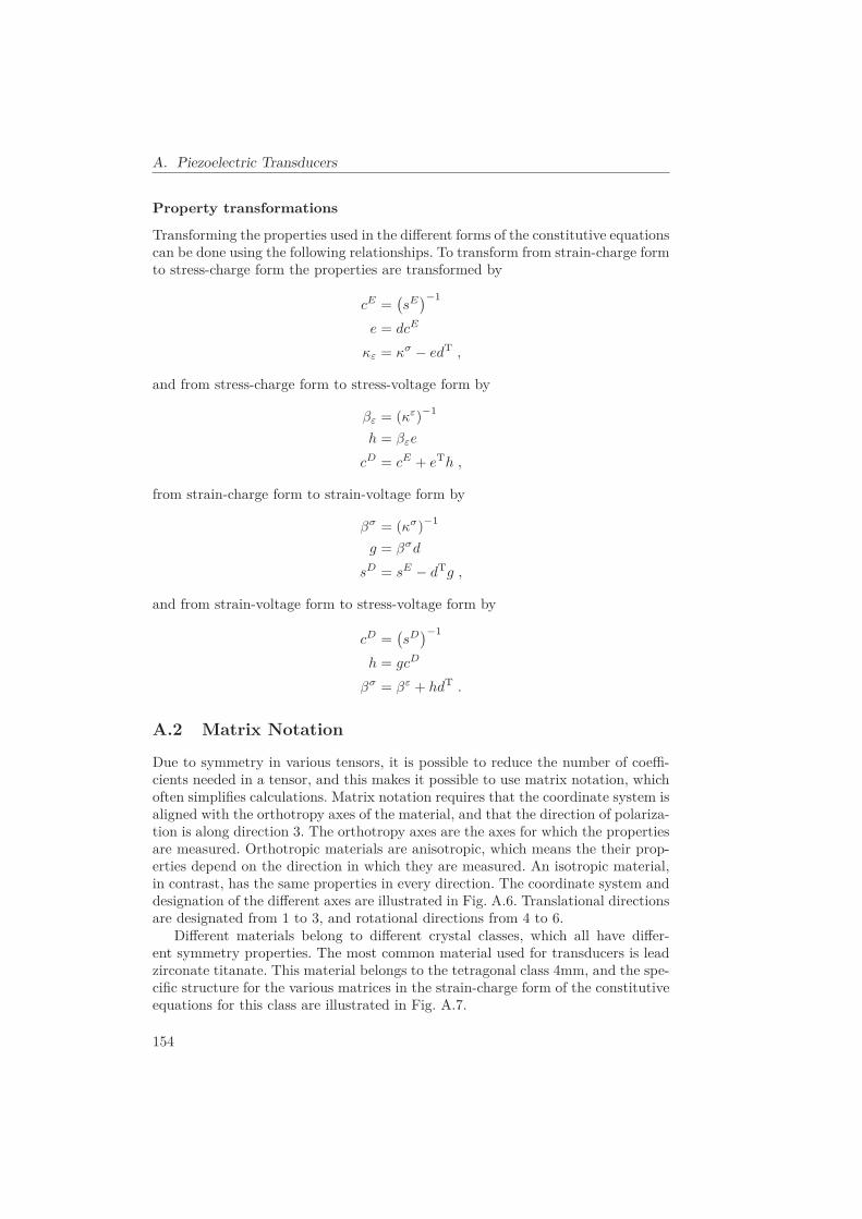
A. Piezoelectric Transducers
Property transformations
Transforming the properties used in the different forms of the constitutive equationscan be done using the following relationships. To transform from strain-charge formto stress-charge form the properties are transformed by
cE =(sE)−1
e = dcE
κε = κσ − edT ,
and from stress-charge form to stress-voltage form by
βε = (κε)−1
h = βεe
cD = cE + eTh ,
from strain-charge form to strain-voltage form by
βσ = (κσ)−1
g = βσd
sD = sE − dTg ,
and from strain-voltage form to stress-voltage form by
cD =(sD)−1
h = gcD
βσ = βε + hdT .
A.2 Matrix Notation
Due to symmetry in various tensors, it is possible to reduce the number of coeffi-cients needed in a tensor, and this makes it possible to use matrix notation, whichoften simplifies calculations. Matrix notation requires that the coordinate system isaligned with the orthotropy axes of the material, and that the direction of polariza-tion is along direction 3. The orthotropy axes are the axes for which the propertiesare measured. Orthotropic materials are anisotropic, which means the their prop-erties depend on the direction in which they are measured. An isotropic material,in contrast, has the same properties in every direction. The coordinate system anddesignation of the different axes are illustrated in Fig. A.6. Translational directionsare designated from 1 to 3, and rotational directions from 4 to 6.
Different materials belong to different crystal classes, which all have differ-ent symmetry properties. The most common material used for transducers is leadzirconate titanate. This material belongs to the tetragonal class 4mm, and the spe-cific structure for the various matrices in the strain-charge form of the constitutiveequations for this class are illustrated in Fig. A.7.
154
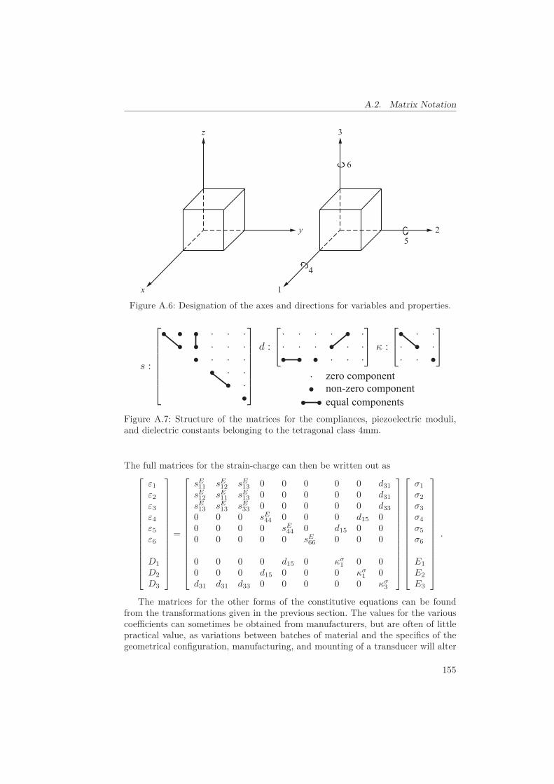
A.2. Matrix Notation
z
x
y
3
1
2
4
5
6
Figure A.6: Designation of the axes and directions for variables and properties.
zero componentnon-zero componentequal components
Figure A.7: Structure of the matrices for the compliances, piezoelectric moduli,and dielectric constants belonging to the tetragonal class 4mm.
The full matrices for the strain-charge can then be written out as⎡⎢⎢⎢⎢⎢⎢⎢⎢⎢⎢⎢⎢⎢⎢⎣
ε1ε2ε3ε4ε5ε6
D1D2D3
⎤⎥⎥⎥⎥⎥⎥⎥⎥⎥⎥⎥⎥⎥⎥⎦=
⎡⎢⎢⎢⎢⎢⎢⎢⎢⎢⎢⎢⎢⎢⎢⎣
sE11 sE
12 sE13 0 0 0 0 0 d31
sE12 sE
11 sE13 0 0 0 0 0 d31
sE13 sE
13 sE33 0 0 0 0 0 d33
0 0 0 sE44 0 0 0 d15 0
0 0 0 0 sE44 0 d15 0 0
0 0 0 0 0 sE66 0 0 0
0 0 0 0 d15 0 κσ1 0 0
0 0 0 d15 0 0 0 κσ1 0
d31 d31 d33 0 0 0 0 0 κσ3
⎤⎥⎥⎥⎥⎥⎥⎥⎥⎥⎥⎥⎥⎥⎥⎦
⎡⎢⎢⎢⎢⎢⎢⎢⎢⎢⎢⎢⎢⎢⎢⎣
σ1σ2σ3σ4σ5σ6
E1E2E3
⎤⎥⎥⎥⎥⎥⎥⎥⎥⎥⎥⎥⎥⎥⎥⎦
.
The matrices for the other forms of the constitutive equations can be foundfrom the transformations given in the previous section. The values for the variouscoefficients can sometimes be obtained from manufacturers, but are often of littlepractical value, as variations between batches of material and the specifics of thegeometrical configuration, manufacturing, and mounting of a transducer will alter
155

A. Piezoelectric Transducers
sE11 12.3 10−12 m2/N
sE33 15.5
sE44 39.0
sE66 32.7
sE12 -4.05
sE13 -5.31
d31 -123 10−12 m/Vd33 289d15 496
κσ1 /κ0 1475 κ0 = 8.854 · 10−12 F/m
κσ3 /κ0 1300ρ 7.5 103 kg/m3
Curie point 328 ◦C
Table A.1: Typical properties of one type of lead zirconate titanate (PZT-4).
the properties actually observed. The parameters will also change with tempera-ture, the frequency of applied stimuli, and due to depolarization. Also, some ofthe coefficients are not actually constant, notably the permittivity κ. The electricdisplacement is determined by the polarization P , which when assuming that thematerial is isotropic with regards to this property is given as
P = κ0χE ,
where χ is the dielectric susceptibility. The electric displacement is therefore givenas
D = κ0E + P = κ0(1 + χ)E = κE .
The dielectric susceptibility for ferroelectric materials can only be considered con-stant when used in a small-signal model. It can not be considered a constant whenthere are large variations of the electric field intensity E. In those cases it is rathera function of the electric field intensity, and this is the cause of hysteresis. An indi-cation of the small-signal behavior, compared to the large-signal behavior, can beinferred from Fig. 1.2b.
As an example, some typical property values of one type of lead zirconatetitanate (PZT-4) are presented in Tab. A.1.
A.3 Stack Actuator Blocking Force
As an example of how to perform calculations using the tensor relationships pre-sented, the expression for the blocking force for a piezoelectric stack actuator foundin the following.
156
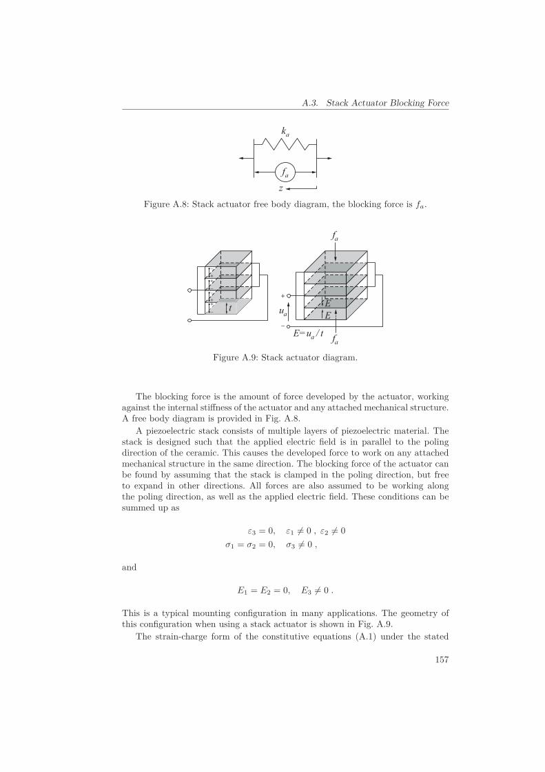
A.3. Stack Actuator Blocking Force
zfa
ka
Figure A.8: Stack actuator free body diagram, the blocking force is fa.
ua
+
–
fa
fa
t+–
–+
+–
–+
E = ua / t
EE
Figure A.9: Stack actuator diagram.
The blocking force is the amount of force developed by the actuator, workingagainst the internal stiffness of the actuator and any attached mechanical structure.A free body diagram is provided in Fig. A.8.
A piezoelectric stack consists of multiple layers of piezoelectric material. Thestack is designed such that the applied electric field is in parallel to the polingdirection of the ceramic. This causes the developed force to work on any attachedmechanical structure in the same direction. The blocking force of the actuator canbe found by assuming that the stack is clamped in the poling direction, but freeto expand in other directions. All forces are also assumed to be working alongthe poling direction, as well as the applied electric field. These conditions can besummed up as
ε3 = 0, ε1 �= 0 , ε2 �= 0σ1 = σ2 = 0, σ3 �= 0 ,
and
E1 = E2 = 0, E3 �= 0 .
This is a typical mounting configuration in many applications. The geometry ofthis configuration when using a stack actuator is shown in Fig. A.9.
The strain-charge form of the constitutive equations (A.1) under the stated
157

A. Piezoelectric Transducers
conditions yield
ε1 = sE13σ3 + d31E3 (A.9)
ε2 = sE13σ3 + d31E3, (A.10)
while from the stress-charge form (A.3), the stress in the poling direction is ex-pressed as
σ3 = cE13ε1 + cE
13ε2 − e33E3. (A.11)
Substituting (A.9) and (A.10) into (A.11) yields
σ3 = 2cE13(sE
13σ3 + d31E3)− (
2d31cE13 + d33cE
33)
E3 = 2cE13sE
13σ3 − d33cE33E3 ,
sincee33 = 2d31cE
13 + d33cE33 .
This provides the stress on an element in the poling direction as
σ3 = −d33(cE
33 − 2cE13ν
)E3.
where ν is (the dimensionless) Poisson’s ratio
ν = −ε1
ε3= −ε2
ε3= −sE
13σ3
sE33σ3
= −sE13
sE33
=cE
13cE
11 + cE12
,
since
sE13 =
cE13
2(cE13)2 − cE
33(cE11 + cE
12),
sE33 = − cE
11 + cE12
2(cE13)2 − cE
33(cE11 + cE
12).
The geometry of one stack element should be well approximated by a rectangu-lar cuboid, with length, or thickness, t, and having a surface area of A for the facesnormal to the direction of the length. Any forces working on an attached mechan-ical structure should be distributed over these faces, and any voltage applied overelectrodes on these faces, must be distributed over the thickness. The stress on theelement due to a force fa in the poling direction, distributed over the surface areaA, should therefore be
σ3 =fa
A,
and electric field due to the applied voltage ua over the thickness t of the elementis
E3 =ua
t.
In a static configuration there should now be a balance of stress in the element as
fa
A= −d33
(cE
33 − 2cE13ν
) ua
t,
158

A.4. Charge in Actuator Circuit
and thus the blocking force developed by the piezoelectric element is
fa = −d33
[(cE
33 − 2cE13ν
)A
t
]ua .
If n elements are stacked on top of each other with each of them having the thicknesst = �/n, � being the length of the stack, and if it is recognized that the stiffness ofthe stack will be given as
ka =(cE
33 − 2cE13ν
)A
�(N/m) ,
an expression for the developed blocking force for a stack actuator is obtained as
fa = −nd33kaua . (A.12)
By also allowing motion along the poling direction, ε �= 0, the stress, σ3, canbe found as
σ3 =(cE
33 − 2cE13ν
)ε3 − d33
(cE
33 − 2cE13ν
)E3 . (A.13)
Since the strain of the element is defined as the ratio of the increase in length, ordisplacement, w, of the element, and the original length, t. That is,
ε3 =w
t,
and (A.13) can be put on the form
fa = kaw − nd33kaua . (A.14)
A.4 Charge in Actuator Circuit
As another example, the expression for the charge in the actuator circuit is foundfor a piezoelectric stack. From the strain-charge form of the constitutive equationsthe generated electric displacement in the poling direction of a piezoelectric elementis found when
ε1 �= 0 , ε2 �= 0 , ε3 �= 0σ1 = σ2 = 0, σ3 �= 0
E1 = E2 = 0, E3 �= 0
asD3 = d33σ3 + κσ
33E3 . (A.15)
Here, the stack is also allowed to move along direction 3. The strains ε1 and ε2 dueto a uniaxial stress σ3 on the element can be found using Hooke’s law as
ε1 = sE13σ3
ε2 = sE13σ3 ,
159

A. Piezoelectric Transducers
and these relationships can be used to solve for the resulting stress σ3 due to thestrain ε3 as
σ3 = cE13ε1 + cE
13ε2 + cE33ε3 = 2cE
13sE13σ3 + cE
33ε3 ,
which yieldsσ3 =
(cE
33 − 2cE13ν
)ε3 , (A.16)
where ν is Poisson’s ratio. The strain of the element is defined as the ratio of theincrease in length, or displacement, w, of the element, and the original length, t.That is,
ε3 =w
t.
The generated charge q on the surface area A of the n rectangular cuboidelements will be
q = nAD3 . (A.17)
Thus, using (A.15), yields
q = nA (d33σ3 + κσ33E3) . (A.18)
Substituting in the expressions (A.16), ε3 = w/t, E3 = ua/t, and t = �/n yields
q = nA(d33
(cE
33 − 2cE13ν
)ε3 + κσ
33E3)= nd33kaw +
κσ33A
�ua ,
whereCp =
κσ33A
�(C/V)
is recognized as the capacitance of the stack. The expression for the charge in theactuator circuit is therefore
q = nd33kaw + Cpua . (A.19)
A.5 One-Dimensional Transducers
As previously noted, the values for the various coefficients as obtained from datasheets provided by manufacturers are often not accurate, and the actual observedresponse from a system is dependent on the specifics of the geometrical configu-ration, manufacturing, and mounting of a transducer. Property values also changewith temperature, and due to depolarization, or aging, and other factors. Trans-ducers are also typically always working with regards to one direction only. Theinterconnection with other systems produce lumped parameter expressions, whereindividual identification of various parameters in the expression might be impossi-ble. From a practical perspective, it is therefore convenient to regard all transduc-ers to be one-dimensional, with unknown parameters. The derivation of models arethen much simplified, and system identification can be done once a model structureis determined.
160

A.5. One-Dimensional Transducers
As the two examples in the previous Sections show, the stress-charge form ofthe constitutive equations can, for a stack actuator operating in one direction, beput on the form [
fa
q
]=[ka −ea
ea Cp
] [wua
], (A.20)
where ea = nd33ka (N/V = C/m). Similarly, the strain-charge form can be ex-pressed as [
wq
]=[1/ka da
da Cp(1 + k2)
] [fa
ua
], (A.21)
where da = ea/ka (m/V = C/N), and
k2 =n2d33
2ka
Cp, (A.22)
which is a constant sometimes used in the literature, called the electromechani-cal coupling factor. It provides a measure of the ratio of energy converted fromelectrical to mechanical energy, or vice versa, i.e., it is an efficiency measure.
161

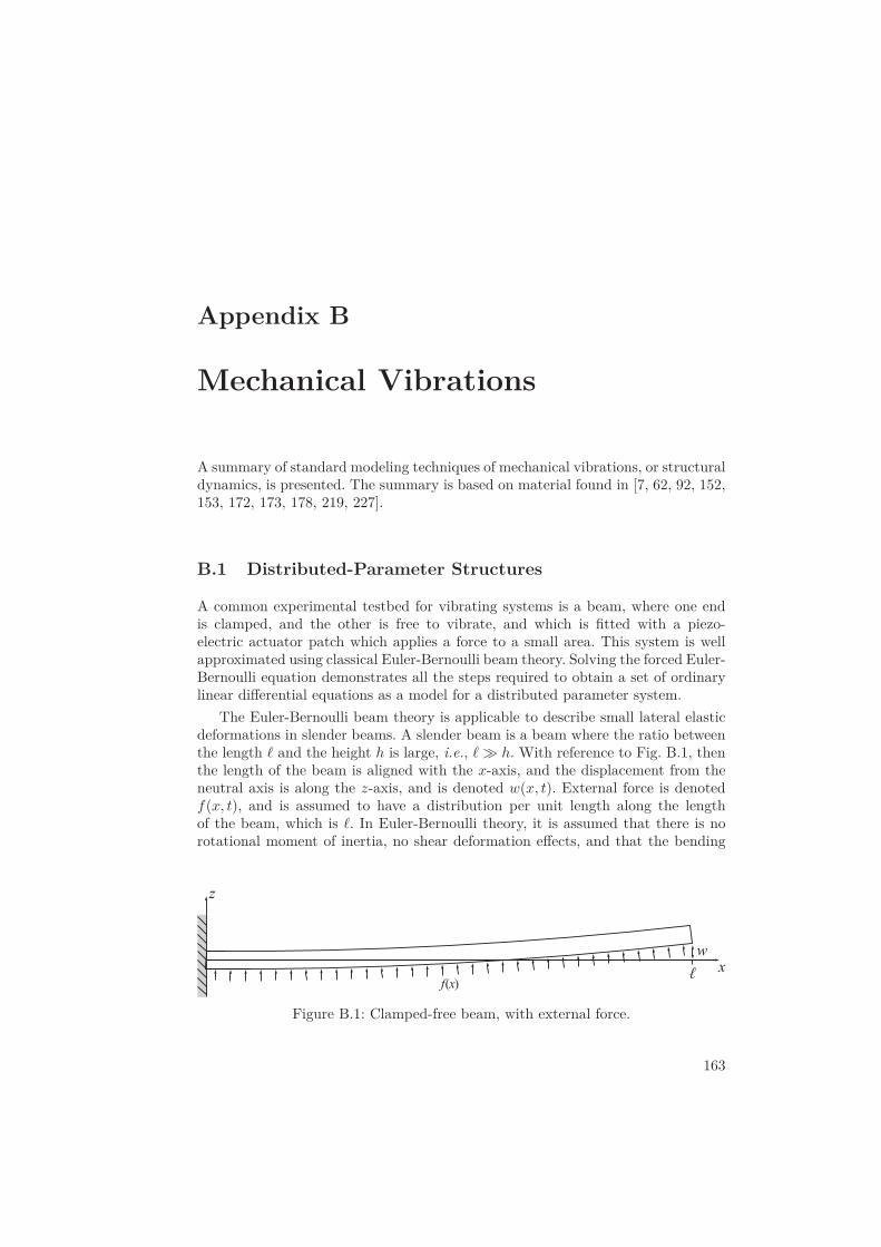
Appendix B
Mechanical Vibrations
A summary of standard modeling techniques of mechanical vibrations, or structuraldynamics, is presented. The summary is based on material found in [7, 62, 92, 152,153, 172, 173, 178, 219, 227].
B.1 Distributed-Parameter Structures
A common experimental testbed for vibrating systems is a beam, where one endis clamped, and the other is free to vibrate, and which is fitted with a piezo-electric actuator patch which applies a force to a small area. This system is wellapproximated using classical Euler-Bernoulli beam theory. Solving the forced Euler-Bernoulli equation demonstrates all the steps required to obtain a set of ordinarylinear differential equations as a model for a distributed parameter system.
The Euler-Bernoulli beam theory is applicable to describe small lateral elasticdeformations in slender beams. A slender beam is a beam where the ratio betweenthe length � and the height h is large, i.e., � � h. With reference to Fig. B.1, thenthe length of the beam is aligned with the x-axis, and the displacement from theneutral axis is along the z-axis, and is denoted w(x, t). External force is denotedf(x, t), and is assumed to have a distribution per unit length along the lengthof the beam, which is �. In Euler-Bernoulli theory, it is assumed that there is norotational moment of inertia, no shear deformation effects, and that the bending
xw
z
f(x)
Figure B.1: Clamped-free beam, with external force.
163

B. Mechanical Vibrations
moment is given by the constitutive equation
Y I(x)∂2w
∂x2 (x, t) , (B.1)
where Y is Young’s modulus, and I(x) is the moment of inertia about the y-axis.Young’s modulus describes the response of some material to linear strain, and istherefore generalized by the elastic stiffness tensor c.
Combining the force and moment balance for an infinitesimal element of thebeam and using the Euler-Bernoulli assumptions yields the partial differential equa-tion
∂2
∂x2
[Y I(x)
∂2w
∂x2 (x, t)]+ ρ(x)
∂2w
∂t2 (x, t) = f(x, t) , (B.2)
where ρ(x) is the mass density of the beam. Now, if in addition it is assumed thatthe moment of inertia is constant, that there is a linear distribution of mass, andthat a force u(t) is applied at a point xu, i.e.,
f(x, t) = δ(x − xu)u(t) , (B.3)
where δ(x) is the Dirac delta, then the equation becomes
ρcs2 ∂4w
∂x4 (x, t) + ρ∂2w
∂t2 (x, t) = δ(x − xu)u(t) , cs2 =
Y I
ρ. (B.4)
Eq. (B.4) can be solved in two steps. First, the unforced solution is found, i.e.,when f(x, t) = 0, by assuming the solution is on the form
w(x, t) =∞∑
i=1
qi(t)φi(x) . (B.5)
Substituting (B.5) into (B.4) yields expressions on the form
cs2φ
(4)i (x)qi(t) + φi(x)qi(t) = 0 (B.6)
which can be solved by separation of variables, that is, by solving the two ordinarydifferential equations
cs2 φ
(4)i (x)φi(x)
= − qi(t)qi(t)
= Ki , (B.7)
where Ki > 0 is a constant, as it must satisfy both differential equations simulta-neously. Defining the constant as Ki = ωi
2 = cs2λi
4, the two differential equationscan be expressed as
qi(t) + ωi2qi(t) = 0 , (B.8)
andφ
(4)i (x) − λi
4φi(x) = 0 . (B.9)
Eq. (B.8) is the differential equation for an harmonic oscillator, while the generalsolution to (B.9) is given by
φi(x) = Ai cosλix + Bi sinλix + Ci coshλix + Di sinhλix , (B.10)
164

B.1. Distributed-Parameter Structures
and φi(x) is called a shape function. The coefficients Ai, Bi, Ci, Di of (B.10) dependon the boundary conditions of the partial differential equation. For the case whenthere is one clamped end and one free end, the boundary conditions for the clampedend are
w(0, t) = 0 ,∂w
∂x(0, t) = 0 , (B.11)
which means it has zero elastic deformation and zero elastic angle, and for the freeend they are
∂w2
∂x2 (�, t) = 0 ,∂w3
∂x3 (�, t) = 0 , (B.12)
which means that it has zero bending moment and zero shear force. By differenti-ating (B.10) and equating with the boundary conditions, a set of linear equationsis obtained, which is⎡⎢⎢⎣
1 0 1 00 1 0 1
− cosλi� − sinλi� coshλi� sinhλi�sinλi� − cosλi� sinhλi� coshλi�
⎤⎥⎥⎦
︸ ︷︷ ︸Acf
⎡⎢⎢⎣
Ai
Bi
Ci
Di
⎤⎥⎥⎦
︸ ︷︷ ︸bc
=
⎡⎢⎢⎣
0000
⎤⎥⎥⎦
︸ ︷︷ ︸0
=
⎡⎢⎢⎣
φ(0)φ′(0)φ′′(�)φ′′′(�)
⎤⎥⎥⎦ .
(B.13)Non-trivial solutions of the equations Acf bc = 0 are found when detAcf = 0, i.e.,
1 + cosλi� coshλi� = 0 . (B.14)
This is a transcendental equation with infinitely many solutions {λi}, which definesthe set {Ai, Bi, Ci, Di}. The solutions {λi} must be found numerically, or can befound in standard tables. The numerical values for the clamped-free case are:
λ1� ≈ 1.8751041λ2� ≈ 4.69409113λ3� ≈ 7.85475743λ4� ≈ 10.99554074λ5� ≈ 14.13716839
λi� ≈ (2i − 1)π2
, i > 5
For each λi, there is also a corresponding natural frequency in (B.8) whichis ωi = csλi
2. It might be noted that for increasingly higher modes, the accuracyof the predicted modes is reduced. This is because the rotation of a infinitesimalbeam element can no longer be considered negligible compared to the translationfor higher order modes, as the curvature for the modes becomes more severe. Thiswill therefore invalidate the Euler-Bernoulli assumptions.
For the shape function φi(x), the coefficients Ai, Bi, Ci, Di for the clamped-freebeam can be expressed in terms of Ai using Ci = −Ai, Di = −Bi, and
Bi = αiAi , αi = −cosλi� + coshλi�
sinλi� + sinhλi�, (B.15)
165

B. Mechanical Vibrations
0 0.1 0.2 0.3 0.4 0.5 0.6 0.7 0.8 0.9 1
0
1
2
x
i(x)
1(x)
2(x)
3(x)
Figure B.2: The first three shape functions for a clamped-free beam of unit length.
such thatφi = Ai [cosλix − coshλix + αi(sinλix − sinhλix)] . (B.16)
The first three shape functions for the clamped-free case are shown in Fig. B.2 fora beam of unit length and Ai = 1.
Normalizing the coefficients Ai such that
∫ �
0ρ[φi(x)]2 dx = 1 (B.17)
the complete solution to the initial value problem is given by (B.5), (B.16), and
qi(t) = qi(0) cosωit . (B.18)
For specified boundary conditions, the solutions {φi(x)} are called eigenfunc-tions of (B.9), and it can be shown that they are orthogonal in the sense that theysatisfy, if they are normalized according to (B.17),
∫ �
0ρ[φi(x)φj(x)] dx = δij , (B.19)
and ∫ �
0ρ[φ′′
i (x)φ′′j (x)] dx = λiδij , (B.20)
where δij is the Kronecker delta.Next, the forced solution is found. As the solution is assumed to be on the
form (B.5), the partial differential equation (B.4) can be expressed as
∞∑j=1
ρcs2qj(t)φ
(4)j (x) + ρqj(t)φj(x) = δ(x − xu)u(t) . (B.21)
166

B.1. Distributed-Parameter Structures
Substituting in (B.9), i.e., φ(4)j (x) = λj
4φj(x), and using ωj2 = cs
2λj4, yields
∞∑j=1
ρφj(x)[ωj
2qj(t) + qj(t)]= δ(x − xu)u(t) . (B.22)
Now, by using the Galerkin method, (B.22) is multiplied by φi(x) and integratedover the domain x ∈ [0, �], which yields
∫ �
0φi(x)
∞∑j=1
ρφj(x)[ωj
2qj(t) + qj(t)]dx =
∫ �
0φi(x)δ(x − xu)u(t) dx . (B.23)
Using the orthogonality property (B.19), and the fact∫∞
−∞ = h(x)δ(x − a) = h(a),yields
ωi2qi(t) + qi(t) = φi(xu)u(t) , (B.24)
which has the Laplace transform
qi(s) =φi(xu)
s2 + ωi2 u(s) . (B.25)
If the displacement is measured at a point xy along the beam,
y(t) = w(xy, t) , (B.26)
the transfer-function from the applied force can be found to be, using (B.5),
G(s) =y
u(s) =
∞∑i=1
φi(xy)φi(xu)s2 + ωi
2 . (B.27)
If the applied force, or actuator, and the measurement, or sensor, are co-located,that is if xy = xu = x0, the transfer-function (B.27) have some special properties.The Fourier transform is then
G(jω) =∞∑
i=1
βi
ωi2 − ω2 . (B.28)
where βi = φi(x0)2, which is the square of the value of the shape function atthe chosen point x0. The function (B.28) is real valued and have infinitely manysingular points where
limω→ωi
−G(jω) = +∞
andlim
ω→ωi+
G(jω) = −∞
and sinceddω
G(jω) =∞∑
i=1
2βiω
(ω2i − ω2)2
> 0 ∀ ω > 0 (B.29)
167

B. Mechanical Vibrations
1 z1 2 z2 3
G(j
)
Figure B.3: The real valued Fourier transform G(jω) of the transfer-function G(s).
|G(j
)|
1 z1 2 z2 3
0
G(j
)
(dB
)
Figure B.4: The gain and phase diagram for the transfer-function G(s).
the function G(jω) is monotonously increasing between each singular point. Thismeans that (B.27) has infinitely many poles {ωi} and zeros {zi}, and, as illustratedin Fig. B.3, the poles and zeros are interleaved, i.e.,
ω1 < z1 < ω2 < z2 < ω3 ... (B.30)
which renders a phase angle ∠G(jω) that is always between -180◦ and 0◦, as illus-trated in Fig. B.4.
Also, if the measurement is velocity, that is, if y(t) = w(xy, t) is measured, then
168

B.2. Lumped-Parameter Structures
w1
m1 m2 m3
k1 k2 k3
d1d2 d3
mn-1 mn
kn
dnw2 w3 wn-1 wn
Figure B.5: Clamped-free point masses, with generalized external force.
the transfer-function is
H(s) =y
u(s) =
∞∑i=1
sβi
s2 + ωi2 . (B.31)
This can be seen to be a passive, or positive real, transfer-function, as each termof the sum is (marginally) stable and has relative degree one, i.e., the phase angle∠H(jω) is always between -90◦ and 90◦, and this is therefore equivalent to a parallelinterconnection of passive systems.
If the actuator and sensor are not co-located, i.e., xy �= xu, it may be that φi(xy)and φi(xu) have opposite signs for certain i. In this case the transfer-function G(s)will no longer satisfy the pole-zero interleaving property, and H(s) will no longerbe passive.
The location of the actuator and sensor is also of significance for two additionalreasons. If the actuator is located at a point xu where φi(xu) = 0, then the controlinput u(t) will have no influence on the mode i. This is equivalent to having amode that is not controllable. Similarly, if the sensor is located at a point xy whereφi(xy) = 0, then the mode i will not be noticeable in the measurement y, which isequivalent to having a mode that is not observable.
B.2 Lumped-Parameter Structures
It is usually not feasible to work with an infinite series on the form (B.27), andmodels derived using continuum mechanics tend to reduce in accuracy for higherorder modes. Discrete lumped mass models of finite order n is often used as anapproximation, and an example of such a system is shown in Fig. B.5. Such modelscan be found by, e.g., spatial discretization using finite element methods, by trun-cating the expression in (B.27), or by parameter identification using experimentaltime-series or frequency data.
The general expression for the equations of motion governing the dynamic re-sponse of non-gyroscopic, discrete, flexible structure with a finite number of degreesof freedom is
Mw + Dw + Kw = τ(t) , (B.32)
where M is the real positive definite and symmetric mass matrix, while D and Kare the real positive semi-definite and symmetric damping and stiffness matrices,respectively. Here, w denotes the vector of generalized displacements, and τ(t) is a
169

B. Mechanical Vibrations
vector of generalized forces. With respect to the structure in Fig. B.5, the dynamicscan be described using a mass matrix on the form
M =
⎡⎢⎢⎢⎢⎢⎣
m1 0 0 00 m2 0 · · · 00 0 m3 0
.... . . 0
0 0 0 0 mn
⎤⎥⎥⎥⎥⎥⎦ ,
a stiffness matrix on the form
K =
⎡⎢⎢⎢⎢⎢⎢⎣
k1 + k2 −k2 0 0−k2 k2 + k3 −k3 · · · 0
0 −k3. . .
...... kn−1 + kn −kn
0 0 · · · −kn kn
⎤⎥⎥⎥⎥⎥⎥⎦ ,
and a damping matrix on the form
D =
⎡⎢⎢⎢⎢⎢⎢⎣
d1 + d2 −d2 0 0−d2 d2 + d3 −d3 · · · 0
0 −d3. . .
...... dn−1 + dn −dn
0 0 · · · −dn dn
⎤⎥⎥⎥⎥⎥⎥⎦ .
The damping matrix is used to model energy dissipation, but dissipation mecha-nisms are often not well known. The classical dissipation model is Rayleigh damp-ing, in which case the damping matrix has the form
D = αM + βK . (B.33)
With regards to the structure in Fig. B.5, Rayleigh damping corresponds to thecase when α = 0.
The undamped natural frequencies {ωi} can be found from the eigenvalue prob-lem
(M−1K − ωi2I)φi = 0 ,
where φi is the associated eigenvector to the eigenvalue ωi2. Since M is positive def-
inite and K is positive semi-definite, M−1K is diagonalizable and has non-negativeeigenvalues. Assuming that the eigenvalues are non-repeated, an eigenvector basiscan be found as
Φ = [φ1, φ2, · · · , φn] .
It is common, however, to solve the eigenvalue problem using Cholesky decompo-sition. Then the mass matrix is decomposed into
M = LLT , (B.34)
170
B.2. Lumped-Parameter Structures
where L is a lower triangular non-singular real matrix. The eigenvalue problem canthen be restated using
φi = L−Tpi (B.35)
as(L−1KL−T − ωi
2I)pi = 0 , (B.36)
where L−1KL−T is a real symmetric matrix. Assuming that the eigenvalues arenon-repeated, another eigenvector basis can be found as
P = [p1, p2, · · · , pn] ,
which in addition is orthogonal, since L−1KL−T a real symmetric matrix. Theeigenvalues are the same for M−1K and L−1KL−T, but the eigenvectors are dif-ferent. Normalizing the eigenvectors such that
P TP = I , (B.37)
then the basis becomes orthonormal, and the matrix L−1KL−T is then diagonalizedas
P −1(L−1KL−T)P = Ω2 . (B.38)
Since Ω2 is diagonal, it has a principal square root Ω, where the undamped naturalfrequencies {ωi} appear on the diagonal, i.e.,
Ω = diag{ωi} . (B.39)
The relation between the Φ and P is given by
Φ = L−TP , (B.40)
and Φ is called the modal matrix, and it is orthonormal with respect to the massmatrix, as well as orthogonal with respect to the stiffness matrix, i.e.,
ΦTMΦ = I (B.41)
andΦTKΦ = Ω2 . (B.42)
If Rayleigh damping is assumed, the similarity transform defined by Φ can be usedto find the modal damping ratios {ζi} on the diagonal of the diagonal matrix
Z =12(αΩ−1 + βΩ
)= diag{ζi} . (B.43)
This follows fromΦTDΦ = αI + βΩ2 = 2ZΩ . (B.44)
Now, by using the similarity transform defined by Φ, the displacement vectorw can be transformed to the modal coordinates q using
w = Φq , (B.45)
171

B. Mechanical Vibrations
and this puts the equations of motion on the form
q + 2ZΩq +Ω2q = Φ−1τ(t) . (B.46)
Taking the Laplace transform of (B.46), yields
q(s) = [Is2 + 2ZΩs +Ω2]−1ΦTτ(s) , (B.47)
where, due to the fact that Z and Ω are diagonal matrices,
[Is2 + 2ZΩs +Ω2]−1 = diag{
1s2 + 2ζiωis + ωi
2
}. (B.48)
Now, since w = Φq, the Laplace transform of (B.32) can be expressed as
G(s) =w
τ(s) = Φ[s2I + s2ZΩs +Ω2]−1ΦT , (B.49)
which due to the diagonal matrix (B.48) can again be written as
G(s) =n∑
i=1
φiφiT
s2 + 2ζiωis + ωi2 . (B.50)
This is analogous to (B.27) (for the case when there is no damping), i.e., thesystem is a parallel interconnection of independent mass-spring-damper systems.The index into the transfer transfer matrix, e.g., Gkl(s), expresses an input-outputrelationship, determining the response of degree of freedom k to a force applied atdegree of freedom l. For a co-located actuator and sensor pair, k = l. With referenceto the structure in Fig. B.5, there is only one force working on the structure, i.e.,
τ = Bu = [1, 0, 0, · · · , 0]T u , (B.51)
and assuming that there is a co-located sensor, the measured displacement will be
y = w1 = Cw = BTw . (B.52)
The corresponding transfer-function is then given by G11(s), or
y
u(s) = CG(s)B = G11(s) =
n∑i=1
βi
s2 + 2ζiωis + ωi2 , (B.53)
where βi = φi(k)φi(l) = φi(1)2. The transfer-functions for discrete lumped massmodels for co-located actuator and sensor pairs will have the same properties asfor the distributed mass case in the previous section.
In many practical situations, if the model has been obtained using the finiteelement method, or by solving the continuous partial differential equations, themodel is often too large. It is then customary to truncate the model by introducingan approximation to the higher order modes by a static feed-through term R, calleda residual mode. That is, the transfer-function is approximated by
y
u(s) ≈
m∑i=1
βi
s2 + 2ζiωis + ωi2 + R , (B.54)
172

B.3. Some Facts About Second-Order Systems
where
R =n∑
i=m+1
βi
ωi2 , (B.55)
which can be seen to be the static response, or DC-response, of the higher ordermodes. The feed-through term R causes the transfer matrix to become not strictlyproper, and typically improves the accuracy of the predicted zero locations.
B.3 Some Facts About Second-Order Systems
The dynamics of many nanopositioning devices is sufficiently described by a singlemass-spring-damper system. As such, it is of interest to summarize some factsabout such systems, i.e., second-order differential equations.
The dynamics of a non-autonomous mass-spring-damper system is describedby the second-order system
mw + cw + kw = f(t) , (B.56)
where k is the spring constant, c is the damping coefficient, and m is the mass.For this system, the undamped natural (angular) frequency ω0 and damping ratioζ are defined as
ω0 =√
k
mand ζ =
c
2√
mk,
thus, with β0 = 1/m, (B.56) can be written
w + 2ζω0w + ω02w = β0f(t) . (B.57)
For (B.57), the damped natural frequency is found as
ωd = ω0√1 − ζ2 . (B.58)
When u(t) = 0, the system is autonomous. The damped natural frequency is thefrequency an autonomous underdamped system (ζ < 1) will oscillate with given aset of initial values (x0, x0) �= (0, 0).
The resonant frequency for (B.57) is
ωp = ω0√1 − 2ζ2 . (B.59)
The resonant frequency is the frequency at which the non-autonomous system willhave the maximum amplitude response. The amplitude response will only have apeak when 0 ≤ ζ < 1/
√2.
The Laplace transform of (B.57) is
G(s) =β0
s2 + 2ζω0s + ω20
. (B.60)
The amplitude response is found from the Fourier transform (s = jω) as
|G(jω)| = β0√(ω02 − ω2)2 + (2ζω0ω)2
=β0√Δ(ω)
. (B.61)
173

B. Mechanical Vibrations
Differentiating (B.61) with respect to the angular frequency ω yields
ddω
|G(jω)| = −12Δ(ω)−3/2Δ′(ω) ,
whereΔ′(ω) = 4ω(ω2 − ω0
2(1 − 2ζ2)) .
Thus, it should be straight forward to verify that
arg maxω∈R+
|G(jω)| = ωp ,
if 0 < ζ < 1/√2, and if ζ ≥ 1/
√2,
arg maxω∈R+
|G(jω)| = 0 .
For 0 < ζ < 1/√2 the amplitude response at ω = ωp is
|G(jωp)| = β0
2ζω02√1 − ζ2
. (B.62)
174

Appendix C
Hysteresis & Creep Models
This Appendix includes a short introduction to two common frameworks for mod-eling hysteresis, as well as a brief description of two creep models that occur fre-quently in the literature.
The first framework for modeling hysteresis is the class of models that canbe put on the form of the Duhem model. One such model, called the Coleman-Hodgdon model, is discussed very briefly, as this is the model used to develop thehysteresis compensation scheme in Chapter 2. The other framework is the Preisachmodel, which has many features in common with the Prandtl-Ishlinskii model. ThePreisach model is discussed in some detail, in order to illustrate the differences inhow it operates and how it is implemented, compared to the Coleman-Hodgdonmodel.
This Appendix is collated from material found in [45, 46, 53, 58, 114, 135, 146,151, 218].
C.1 Hysteresis
The word hysteresis is derived from Greek, and means “to lag behind”. A commondefinition is that it is a rate-independent, non-linear, multi-branch input-outputmap, where the branching occurs at successive extrema of the input. In manyphysical systems this is seen as the output lagging behind the input between inputextrema, generating loops in the input-output map. The term rate-independentmeans that the branches of such hysteresis non-linearities are determined only bypast extremum values, and not the rate of the input variations. Hysteresis is adynamical relationship, as the output y(t0) at any instant t0 depends on both thecurrent value of the input u(t0) and an internal memory variable. Internal memoryimplies that for equal instantaneous inputs u(t0) = u(t1), different values of theoutput y(t0) �= y(t1) can occur, depending on the state of the internal memory.Due to rate-independence, the input-output map is invariant with respect to timescaling. This means that the input-output relationship y = Hu generates the sameinput-output map for u(t) and u(at + b) for any a, b ∈ R. This is different frommany other types of dynamical systems, which also exhibit a lagging effect, but
175

C. Hysteresis & Creep Models
where the lagging effect is dependent on the rate of input variations. For a lineardynamical system, this would be called phase-lag.
Hysteresis occurs in almost all ferromagnetic and ferroelectric materials. It alsooccurs in other areas, and examples include systems with friction, elastic and su-perconductive materials, adsorption in porous media, and economics.
C.2 The Duhem Model
The Duhem model for hysteresis dates from 1897, in a work by Pierre Duhem, andfocusses on the fact that the output can only change its character when the inputchanges direction. This model uses a phenomenological approach, postulating anintegral operator or differential equation to model a hysteretic relation. A Duhemmodel is given by the general differential equation
η = fI(u, η)(u)+ + fD(u, η)(u)−, η(0) = η0 (C.1)
where the expressions (u)+ and (u)− are interpreted using the definitions
(u)+ :=|u| + u
2
(u)− :=|u| − u
2and which satisfy
(u)+ + (u)− = |u| .
This means that (u)+ = u, u > 0, and (u)+ = 0, u < 0. Conversely, (u)− = 0, u > 0,and (u)− = u, u < 0. The function fI(u, η) then determines the output whenthe input is increasing, and fD(u, η) when the input is decreasing. Models onthe form (C.1) are useful as phenomenological models because the functions andparameters can be fine-tuned to match experimental results in a given situation.
C.2.1 The Coleman-Hodgdon Model
Coleman and Hodgdon have investigated the Duhem model for ferromagnetic hys-teresis, but the model has also been used to describe ferroelectric hysteresis. TheColeman-Hodgdon model, as well as some analysis of the model, is presented inChapter 2. The form of the model studied in Chapter 2 is best suited to describehysteretic responses that are symmetric, and for cases where the input signals varymonotonously between two extremal points.
The model is given as
η = βu − αη|u| + γ|u|u , η(0) = η0 . (C.2)
Thus,fI(u, η) = β − αη + γu and fD(u, η) = β + αη − γu .
Two salient observations from the analysis in Chapter 2, is that the modeldefines branches, and the branching occurs every time the input changes direction.An example of the behavior for the parameter values
α = 0.06 , β = 0.5 , γ = 0.02
176
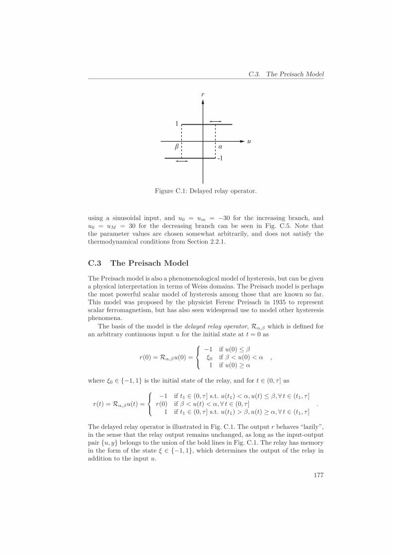
C.3. The Preisach Model
r
u
1
-1
Figure C.1: Delayed relay operator.
using a sinusoidal input, and u0 = um = −30 for the increasing branch, andu0 = uM = 30 for the decreasing branch can be seen in Fig. C.5. Note thatthe parameter values are chosen somewhat arbitrarily, and does not satisfy thethermodynamical conditions from Section 2.2.1.
C.3 The Preisach Model
The Preisach model is also a phenomenological model of hysteresis, but can be givena physical interpretation in terms of Weiss domains. The Preisach model is perhapsthe most powerful scalar model of hysteresis among those that are known so far.This model was proposed by the physicist Ferenc Preisach in 1935 to representscalar ferromagnetism, but has also seen widespread use to model other hysteresisphenomena.
The basis of the model is the delayed relay operator, Rα,β which is defined foran arbitrary continuous input u for the initial state at t = 0 as
r(0) = Rα,βu(0) =
⎧⎨⎩
−1 if u(0) ≤ βξ0 if β < u(0) < α1 if u(0) ≥ α
,
where ξ0 ∈ {−1, 1} is the initial state of the relay, and for t ∈ (0, τ ] as
r(t) = Rα,βu(t) =
⎧⎨⎩
−1 if t1 ∈ (0, τ ] s.t. u(t1) < α, u(t) ≤ β, ∀ t ∈ (t1, τ ]r(0) if β < u(t) < α, ∀ t ∈ (0, τ ]
1 if t1 ∈ (0, τ ] s.t. u(t1) > β, u(t) ≥ α, ∀ t ∈ (t1, τ ].
The delayed relay operator is illustrated in Fig. C.1. The output r behaves “lazily”,in the sense that the relay output remains unchanged, as long as the input-outputpair {u, y} belongs to the union of the bold lines in Fig. C.1. The relay has memoryin the form of the state ξ ∈ {−1, 1}, which determines the output of the relay inaddition to the input u.
177

C. Hysteresis & Creep Models
u(t) w(t)
Figure C.2: Preisach model.
If an infinite set of delayed relay operators is considered, assuming α ≥ β, thenthe Preisach hysteresis model characterizes the output η of a hysteretic system asthe superposition of weighted relays as
η(t) = Hu(t) =∫∫
α≥β
μ(α, β)Rα,βu(t) dα dβ , (C.3)
where μ(α, β) is a weight function, associated with a relay element Rα,β . Eq. (C.3)is illustrated in Fig. C.2. The relay elements represents hysteresis non-linearitieswith local memories, and the memory is represented by the state ξ ∈ {−1, 1}.This can be interpreted as modeling the switching behavior of individual (e.g.,magnetic or electric) dipoles within a material. The weight function μ(α, β) ≥ 0 isan integrable function defined for the half-plane
S = {(α, β) : α ≥ β, α ≤ αm, β ≤ βm} .
The set S is called the Preisach plane, while μ(α, β) is the Preisach density function.For every point (α, β) of S, there exists a unique relay Rα,β .
Assume μ(α, β) has support S, and define, for a given continuous piecewisemonotone input u(·) and time t,
S+(t) = {(α, β) ∈ S : Rα,βu(t) = 1} ,
S−(t) = {(α, β) ∈ S : Rα,βu(t) = −1}.
Then the boundary L(t) = S+(t)∩S−(t), called the Preisach state, is a descending“staircase” with vertices at values of α or β corresponding to a subset of previouslocal maxima or minima of the input u(·), see Fig. C.3. The final link of L(t) isattached to α = β at (u(t), u(t)) by a vertical segment when u(·) is decreasing att, and by a horizontal segment when u(·) is increasing at t. Eg. (C.3) can thereforebe reformulated as
η(t) =∫∫
S+(t)μ(α, β)u(t) dα dβ −
∫∫S−(t)
μ(α, β)u(t) dα dβ .
The operator H is characterized to a large extent by the evolution in time of S+(t),S+(t) and the measure μ(α, β).
178

C.3. The Preisach Model
S +(t)
S –(t)
L(t)
( m, m)
(u(t),u(t))
Figure C.3: Preisach plane.
The Presiach model has two salient properties, which are the wiping out propertyand the congruence property. The wiping out property can be formulated as when-ever u(t) attains a local maximum, all vertices on L(t) with “up”-switching valuesα less than this maximum are wiped out. Conversely, each local minimum of u(·)wipes out all vertices on L(t) with “up”-switching values β greater than this min-imum. So only the alternating dominant input extrema are stored by the Preisachmodel, other input extrema are wiped out. The congruence property means that allprimitive hysteresis loops corresponding to the same extreme values of input arecongruent. If u(t) varies monotonously between two consecutive extremal valuesum and uM , then for all initial states, the resulting loops are congruent. That is,they have the same shape.
To implement the Preisach model numerically, the Preisach plane can be dis-cretized. Perhaps the simplest method for doing this, is to partition S into sub-regions as shown in Fig. C.4. Within each sub-region, the relays are assumed toswitch, up (+1) or down (-1), simultaneously depending on the applied input u(·),and the weighting values μ associated with all the relays in each sub-region are thesame. As a result, the Preisach model (C.3) takes the form
η(t) =nq∑
i=1
μiAiRiu(t) + η0 , (C.4)
where nq represents the total number of sub-regions, μi is the weighting value forthe relay Ri in the ith sub-region of area Ai, and η0 is the bulk contribution tothe output from sub-regions outside of the Preisach plane. If the Preisach planehas been partitioned into nh levels uniformly along the β and α axes, the totalnumber of sub-regions is nq = (nh(nh + 1))/2. The number of relays that needs tobe implemented is therefore nq.
Assuming the possible (α, β) pairs are scaled to accommodate maximum andminimum input values, um and uM , i.e., αm ≥ uM and βm ≤ um, the weights {μi}can be found by sampling the input u and output η of a hysteretic system, in orderto obtain a primitive hysteresis loop. The primitive hysteresis loop is found by
179

C. Hysteresis & Creep Models
1
2
3
4
5
6
7
8
9
10
11
12
13
14 15
Figure C.4: Preisach plane partitioning for nh = 5 levels.
cycling the input monotonously from a minimum um to a maximum uM and backto the minimum uM . Since the Preisach model might not capture all observedeffects in a real hysteretic system, this is best done under stationary conditionsusing a periodic input signal. The resulting time-series {η(tk)} and {u(tk)}, oflength nt, is then used to construct an over-determined system of linear equationson the form⎡⎢⎢⎢⎣
η(t1)η(t2)...
η(tnt)
⎤⎥⎥⎥⎦ =
⎡⎢⎢⎢⎣
A1R1u(t1) A2R2u(t1) . . . AqRqu(t1)A1R1u(t2) A2R2u(t2) . . . AqRqu(t2)
...A1R1u(tnt
) A2R2u(tnt) . . . AqRqu(tnt
)
⎤⎥⎥⎥⎦⎡⎢⎢⎢⎣
μ1μ2...
μnq
⎤⎥⎥⎥⎦+ η0 . (C.5)
This can be put on the more compact form
cη = Aubμ + η0 , (C.6)
where cη is nt × 1, Au is nt × nq, and bμ is nq × 1. The least-squares fit forbμ = [μ1, μ2, ..., μnq
]T is then found using, e.g., the pseudo-inverse as
bμ = Au+(cη − η0) . (C.7)
The input-output map generated by the discrete Preisach model fitted to ahysteresis loop generated using the Coleman-Hodgdon model (C.2) can be seen inFig. C.5. The smooth path is generated by the Coleman-Hodgdon model, and thestaircase formed path is generated by the discrete Preisach model. Here nh = 50levels were used, translating to nq = 1275 relays, thus, the Preisach model becomesorders of magnitude more computationally demanding than the Coleman-Hogdonmodel for reasonable model accuracy.
180
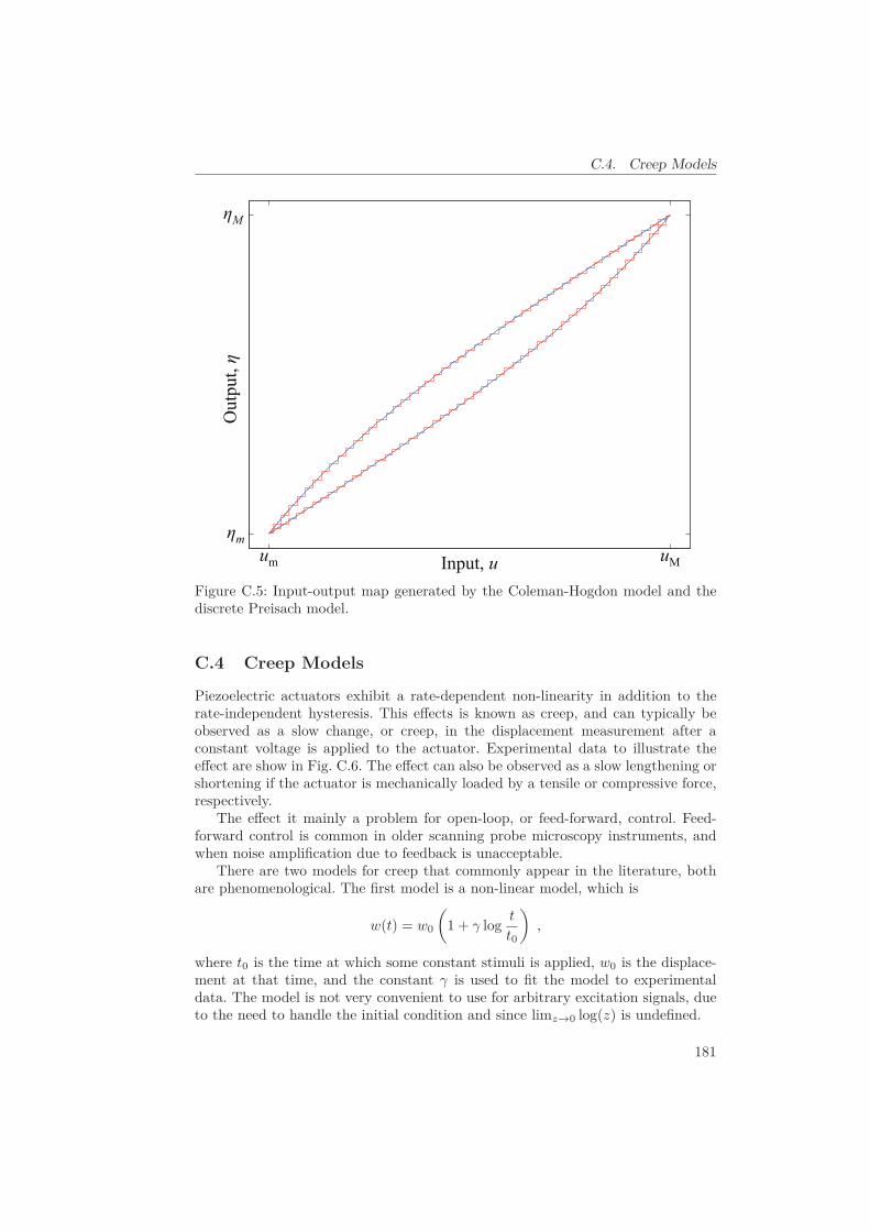
C.4. Creep Models
um uM
m
M
Input, u
Out
put,
Figure C.5: Input-output map generated by the Coleman-Hogdon model and thediscrete Preisach model.
C.4 Creep Models
Piezoelectric actuators exhibit a rate-dependent non-linearity in addition to therate-independent hysteresis. This effects is known as creep, and can typically beobserved as a slow change, or creep, in the displacement measurement after aconstant voltage is applied to the actuator. Experimental data to illustrate theeffect are show in Fig. C.6. The effect can also be observed as a slow lengthening orshortening if the actuator is mechanically loaded by a tensile or compressive force,respectively.
The effect it mainly a problem for open-loop, or feed-forward, control. Feed-forward control is common in older scanning probe microscopy instruments, andwhen noise amplification due to feedback is unacceptable.
There are two models for creep that commonly appear in the literature, bothare phenomenological. The first model is a non-linear model, which is
w(t) = w0
(1 + γ log
t
t0
),
where t0 is the time at which some constant stimuli is applied, w0 is the displace-ment at that time, and the constant γ is used to fit the model to experimentaldata. The model is not very convenient to use for arbitrary excitation signals, dueto the need to handle the initial condition and since limz→0 log(z) is undefined.
181

C. Hysteresis & Creep Models
5 10 15 20 25 30 35
0
2
Time (s)
Dis
plac
emen
t (μm
)
Figure C.6: Piezoelectric actuator creep response to a voltage square-wave.
The second model is more convenient with regards to arbitrary input sig-nals, and consists of a superposition of linear first-order low-pass filters with afeedthrough term, i.e.,
Gc(s) =1k0
+m∑
i=1
1dis + ki
.
This can be considered as a series of springs and dampers, where {k0, ki} are thespring constants and {di} are the damping constants. The first spring constant k0provides the initial static displacement, and the remaining spring-damper elementsmodels the low-frequency creep motion. One advantage of this model is that itis straightforward find the inverse G−1
c (s), and the feed-forward actuation signalcan be found for sufficiently smooth reference signals. Another advantage is thatit can be combined with a model of the vibrational dynamics of the system and beexplicitly accounted for during control design.
182
Appendix D
Online Parameter IdentificationSchemes
The parameter identification schemes used in Chapters 2, 5, and 6 are summarizedbelow. The presentation provides some background and technical details, but isaimed at explaining how the schemes were implemented. This Appendix is collatedfrom material entirely found in [33, 37, 62, 88, 89, 91, 102, 111, 143, 180, 181, 204,207].
D.1 Recursive Least-Squares Method
The least-squares method is perhaps the best known method for parameter iden-tification. It can be used in recursive and non-recursive form. It works by fittingexperimental data to a given model by minimizing the sum of the squares of thedifference between the computed response from the model and the actual measuredresponse. Noise and disturbances in the measured signal is then expected to haveless effect on the accuracy of the resulting parameter estimates.
The starting point is a model of the system, assuming the measured responsez can be described as a vector of model parameters θ appearing affinely with avector of known signals, ϕ, called the regressor,
z = θTϕ . (D.1)
The objective of the method is to find a good estimate of the vector of parametervalues, θ. By computing the estimated response
z = θTϕ
the estimate error ε can be formed as
ε =z − z
m2 (D.2)
where m2 is a normalization signal defined below in (D.4). The (modified) least-squares estimate of the parameters is obtained by minimizing the cost-function
J(θ) =12
∫ t
0e−κf (t−τ)ε2m2 dτ +
12e−κf t(θ − θ0)TQ0(θ − θ0) , (D.3)
183

D. Online Parameter Identification Schemes
where a forgetting factor κf > 0 is introduced to discount past data in order toachieve exponential convergence. The matrix Q0 is used to weigh the significanceof the initial parameter estimates, θ0, in minimizing the cost-function.
The above expressions can be used to derive both the recursive and the non-recursive form of the least-squares method. The recursive form is of interest, as itis amenable to online implementation. The parameter update law is then given by
˙θ = Pεϕ , θ(0) = θ0
The matrix P is called the covariance matrix, and can be found by computing
P ={
κf P − P ϕϕTPm2 , if ‖P‖ ≤ R0
0 otherwise, P (0) = Q−1
0 .
The initial covariance matrix must be symmetric and positive definite, P (0) =Q−1
0 = Q−T0 > 0. By using the forgetting factor κf when updating the covariance
P , there is a possibility for P to grow without bound. To avoid this, some normon P , ‖P‖, is not allowed to grow larger than R0, by stopping the update ofP by setting P = 0. The initial covariance matrix should therefore also satisfy‖P (0)‖ ≤ R0.
The normalization signal m2 can be constructed in various ways. Here it istaken to be
m2 = 1 + ns2, ns
2 = ϕTPϕ . (D.4)
Normalization ensures boundedness of the signals used in the identification scheme.This method is referred to as modified least-squares with forgetting factor. It has
the properties ε, εns, θ,˙θ, P ∈ L∞ and ε, εns,
˙θ ∈ L2. In addition it has the formal
property that if the regressor ϕ is persistently exciting (PE), then θ convergesexponentially to θ.
It should also be noted the to avoid pure numerical differentiation when esti-mating parameters of an linear differential equation of degree n, the output z andregressor vector ϕ should be filtered by a filter with relative degree nf
� ≥ n.
D.1.1 Persistency of Excitation
A piecewise continuous signal vector ϕ : R+ → Rn is said to be persistently exciting
(PE) in Rn with a level of excitation α0 > 0 if there exist constants α1, T0 > 0
such that
α1I ≥ 1T0
∫ t+T0
t
ϕϕT dτ ≥ α0I, ∀t ≥ 0 .
For linear single-input-single-output (SISO) models, a PE regressor vector isobtained if the input signal u is sufficiently rich. In brief, an input signal is suf-ficiently rich if it contains more frequency components than half the number ofunknown parameters in the model.
184

D.2. Integral Adaptive Law
D.2 Integral Adaptive Law
The gradient method based on the integral cost function (integral adaptive law)behaves similarly to the least-squares method, but with the added benefit of a userselectable convergence rate, and it eliminates the need for the initial covariancematrix Q−1
0 .The method recursively minimizes the cost-function
J(θ) =12
∫ t
0e−κf (t−τ)ε2m2 dτ , (D.5)
which is identical to (D.3), except for the term including the inverse of the initialcovariance matrix Q−1
0 . Eq. (D.5) includes the estimate error ε as defined in (D.2),the normalization signal m2 defined below in (D.6), and a forgetting factor κf > 0to discount past data in order to achieve exponential convergence. Applying thegradient method, ˙
θ = −Γ∇J(θ), to find the minimum of (D.5) results in therecursive expressions
˙θ = −Γ(Rθ + Q) , θ(0) = θ0
R = −κf R +ϕϕT
m2 , R(0) = 0
Q = −κf Q − zϕ
m2 , Q(0) = 0
where Γ = ΓT > 0 is the adaptive gain, and the normalization signal m2 is con-structed as
m2 = 1 + ns2 , ns
2 = α0ϕTϕ , α0 > 0 . (D.6)
This method has the properties ε, εns, θ,˙θ, P ∈ L∞, ε, εns,
˙θ ∈ L2, and
limt→∞ | ˙θ| = 0 .
The method has the formal property that if the regressor ϕ is persistently exciting(PE), and ns, ϕ ∈ L∞, then θ will converge exponentially to θ, and for Γ = γ0I,the convergence rate can be made arbitrarily large by increasing the value of γ0.
D.3 Extended Kalman Filter
The extended Kalman filter is a popular method for recursive parameter identifi-cation. It is based on a weighted least-squares criterion, but unlike the recursiveleast-squares method and the integral adaptive law, both the parameters and thestates of the system are estimated.
D.3.1 Continuous Extended Kalman Filter
A general non-linear system is described by
x = f(x, u) + wy = h(x) + v
(D.7)
185

D. Online Parameter Identification Schemes
where x ∈ Rn are the states, y ∈ R
m are the measurements, u ∈ Rl is the input,
and w and v are zero-mean Gaussian white noise processes, described uniquely bythe process noise covariance Qδ(t), and the measurement noise covariance Rδ(t),respectively:
E[w(t)w(τ)T] = Qδ(t − τ)E[v(t)v(τ)T] = Rδ(t − τ)
The extended Kalman filter (EKF) is obtained when the states of the system (D.7)are estimated by linearizing about state trajectory of the filter. Linearization isdone by computing the Jacobians
F =∂f
∂x
∣∣∣∣x
, H =∂h
∂x
∣∣∣∣x
.
Now the state estimates x can be computed by solving
x(0) = E[x(0)]P (0) = E[(x(0) − x(0))(x(0) − x(0))T]
˙x = f(x, u) + K[y − h(x)]K = PHTR−1
P = FP + PF T + Q − KHP ,
where P is the error covariance, and K is the Kalman gain. The above recursionis equivalent to minimizing the cost function
J(x) =12(x − x(0))TP (0)−1(x − x(0))
+12
∫ t
0
((y − h(x))TR−1(y − h(x)) + wTQ−1w
)dτ
subject to x = f(x, u)+w. To summarize; large measurement noise covariance pa-rameters will penalize the use of measurements, and large process noise covarianceparameters will penalize the use of predicted states from the system model. P (0)−1
has the same effect as Q0 in (D.3).The extended Kalman filter can be used for parameter identification by mod-
eling unknown parameters as Wiener processes. Consider the linear system
x = A(θ)x + B(θ)u + w
y = C(θ)x + v
with unknown parameters θ ∈ Rp. By augmenting the state vector to includethe unknown parameters, χT = [xT, θT], the non-linear system χ = f(χ, u) + w,y = h(χ) + v is obtained, where
f(χ, u) =[
A(θ)x + B(θ)u0
]h(χ) = C(θ)x .
186

D.3. Extended Kalman Filter
The Jacobians F and H for this system are found as
F =[
A(θ) ∂∂θ [A(θ)x + B(θ)u]
0 0
]x,θ
,
H =[
C(θ) ∂∂θ [C(θ)x]
]x,θ
.
D.3.2 Hybrid Extended Kalman Filter
When using a numerical integration scheme for solving continuous time differentialequations, a smaller step size should provide more accurate results. Applying acontinuous-discrete, or hybrid, version of the EKF (HEKF) might therefore improvethe accuracy of the estimates, since the continuous part of the method can be runat a higher rate than the sampling rate.
The system response (D.7) is now modified to the hybrid system
x = f(x, uk) + wyk = h(xk) + vk
where yk is sampled sequence of measurements, uk is the input sequence, and vk
is a Gaussian white noise sequence, and the noise properties are given by
E[w(t)w(τ)T] = Qδ(t − τ)E[vkvT
i ] = Rdδki
where Rd ≈ R/Ts, and Ts is the sampling period. Using the initial values
x0 = E[x(0)] and P0 = E[(x(0) − x0)(x(0) − x0)T],
the state estimates xk for k = 1, 2, 3, ... are computed by the hybrid EKF in twoparts.
(1) The a priori state estimates and error covariance, from time-step k − 1 tok− (i.e., for the sampling period Ts), are found by solving
x = f(x, uk−1)P = FP + PF T + Q,
where the initial values are given by x(0) = xk−1 and P (0) = Pk−1.(2) Given the a priori estimates x−
k = x(kTs) and error covariance P −k = P (kTs),
the a posteriori state estimates xk and error covariance Pk are found by computing:
Kk = P −k HT(HP −
k HT + Rd)−1
xk = x−k + Kk(yk − h(x−
k ))Pk = (I − KkH)P −
k (I − KkH) + KkRdKTk
D.3.3 Convergence Properties for the Extended Kalman Filter
For the extended Kalman filter (EKF) there does not exist any general proof ofconvergence. The EKF can provide good performance, but the convergence prop-erties for the estimates are susceptible to the choice of initial values and covariance
187

D. Online Parameter Identification Schemes
tuning, as well as the input signal. As in the case for the recursive least-squaresmethod and the integral adaptive law, the input signal used when applying theEKF must provide sufficient excitation in some sense for the state and parameterestimates to converge. In many practical applications, this happens for signals thatare PE.
188
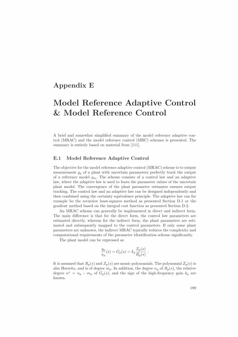
Appendix E
Model Reference Adaptive Control& Model Reference Control
A brief and somewhat simplified summary of the model reference adaptive con-trol (MRAC) and the model reference control (MRC) schemes is presented. Thesummary is entirely based on material from [111].
E.1 Model Reference Adaptive Control
The objective for the model reference adaptive control (MRAC) scheme is to outputmeasurement yp of a plant with uncertain parameters perfectly track the outputof a reference model ym. The scheme consists of a control law and an adaptivelaw, where the adaptive law is used to learn the parameter values of the uncertainplant model. The convergence of the plant parameter estimates ensures outputtracking. The control law and an adaptive law can be designed independently andthen combined using the certainty equivalence principle. The adaptive law can forexample be the recursive least-squares method as presented Section D.1 or thegradient method based on the integral cost function as presented Section D.2.
An MRAC scheme can generally be implemented in direct and indirect form.The main difference is that for the direct form, the control law parameters areestimated directly, whereas for the indirect form, the plant parameters are esti-mated and subsequently mapped to the control parameters. If only some plantparameters are unknown, the indirect MRAC typically reduces the complexity andcomputational requirements of the parameter identification scheme significantly.
The plant model can be expressed as
yp
up(s) = Gp(s) = kp
Zp(s)Rp(s)
.
It is assumed that Rp(s) and Zp(s) are monic polynomials. The polynomial Zp(s) isalso Hurwitz, and is of degree mp. In addition, the degree np of Rp(s), the relativedegree n� = np − mp of Gp(s), and the sign of the high-frequency gain kp areknown.
189

E. Model Reference Adaptive Control & Model Reference Control
3
(s)(s)
(s)(s)
1T
c0 Gp(s)
2T
up
ypr
Figure E.1: The MRAC control law structure.
The reference model
ym
r(s) = Wm(s) = km
Zm(s)Rm(s)
consists of the monic Hurwitz polynomials Zm(s) and Rm(s) of degrees qm andpm, respectively, where pm = np, and the relative degree nm
� = pm − qm = n�.The control law, as shown in Fig. E.1, is given by
up = θ1T α(s)Λ(s)
up + θ2T α(s)Λ(s)
yp + θ3yp + c0r (E.1)
whereα(s) = [snp−2, snp−3, ..., s, 1]T for np ≥ 2α(s) = 0 for np = 1 (E.2)
andΛ(s) = Λ0(s)Zm(s) (E.3)
is a monic and Hurwitz polynomial of degree np − 1. Thus, Λ0(s) is a monic andHurwitz polynomial of degree n0 = np − 1 − qm.
By using the control law structure in Fig. E.1 it is possible to generate therequired signals using the scalar products of the time varying parameters in thevectors θ1 and θ2 and the signal vectors generated by the two linear time invariantfilters given by α(s)
Λ(s) . This greatly simplifies the implementation and the stabilityanalysis of the MRAC scheme.
The control law parameter vector is
θc =[θ1
T, θ2T, θ3, c0
]T
and should be chosen such that the closed-loop complementary sensitivity functionmatches the reference model, i.e.,
yp
r(s) = T (s) = Wm(s) =
ym
r(s) .
190
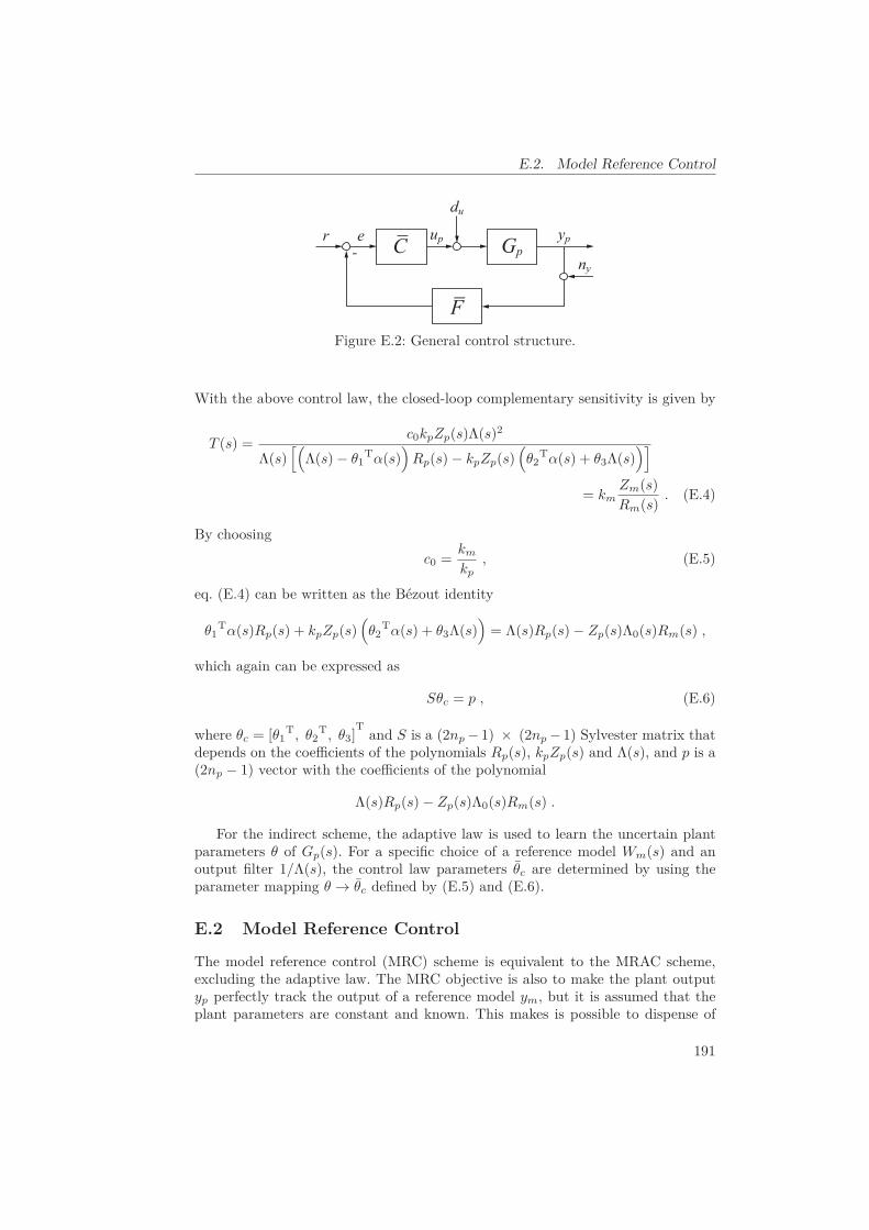
E.2. Model Reference Control
up GpypC
F
r-e
du
ny¯
¯Figure E.2: General control structure.
With the above control law, the closed-loop complementary sensitivity is given by
T (s) =c0kpZp(s)Λ(s)2
Λ(s)[(Λ(s) − θ1
Tα(s))
Rp(s) − kpZp(s)(
θ2Tα(s) + θ3Λ(s)
)]= km
Zm(s)Rm(s)
. (E.4)
By choosing
c0 =km
kp, (E.5)
eq. (E.4) can be written as the Bézout identity
θ1Tα(s)Rp(s) + kpZp(s)
(θ2
Tα(s) + θ3Λ(s))= Λ(s)Rp(s) − Zp(s)Λ0(s)Rm(s) ,
which again can be expressed as
Sθc = p , (E.6)
where θc = [θ1T, θ2
T, θ3]Tand S is a (2np − 1) × (2np − 1) Sylvester matrix that
depends on the coefficients of the polynomials Rp(s), kpZp(s) and Λ(s), and p is a(2np − 1) vector with the coefficients of the polynomial
Λ(s)Rp(s) − Zp(s)Λ0(s)Rm(s) .
For the indirect scheme, the adaptive law is used to learn the uncertain plantparameters θ of Gp(s). For a specific choice of a reference model Wm(s) and anoutput filter 1/Λ(s), the control law parameters θc are determined by using theparameter mapping θ → θc defined by (E.5) and (E.6).
E.2 Model Reference Control
The model reference control (MRC) scheme is equivalent to the MRAC scheme,excluding the adaptive law. The MRC objective is also to make the plant outputyp perfectly track the output of a reference model ym, but it is assumed that theplant parameters are constant and known. This makes is possible to dispense of
191

E. Model Reference Adaptive Control & Model Reference Control
the structure in Fig. E.1, and to use linear time invariant filters exclusively. Thecontrol law can then be expressed in the form of the general control structure inFig. E.2.
The MRC control law is therefore given by
up = C(s)(r − F (s)yp) ,
where C(s) is a feed-forward filter given as
C(s) =c�
0Λ(s)Λ(s) − θ�
1Tα(s)
, (E.7)
and F (s) is a feedback filter given as
F (s) = −θ�2
Tα(s) + θ�3Λ(s)
c�0Λ(s)
. (E.8)
This can be seen from (E.4), since
c�0Λ(s)kpZp(s)(
Λ(s) − θ�1
Tα(s))
Rp − kpZp(s)(
θ�2
Tα(s) + θ�3Λ(s)
)
=c�
0Λ(s)Λ(s)−θ�
1Tα(s) kp
Zp(s)Rp(s)
1 + c�0Λ(s)
Λ(s)−θ�1
Tα(s)
(− θ�
2Tα(s)+θ�
3 Λ(s)c�
0Λ(s)
)kp
Zp(s)Rp(s)
=C(s)Gp(s)
1 + C(s)F (s)Gp(s)= T (s) .
The polynomials α(s) and Λ(s) are still as defined in (E.2) and (E.3), and thefeed-forward and feedback filters are determined by the known plant parametersθ� of Gp(s), the chosen reference model Wm(s) and output filter 1/Λ(s), since thecontrol law parameters θ�
c are determined by using the parameter mapping θ� → θ�c
defined by (E.5) and (E.6).
192

References
[1] Piezoelectric Ceramics – Properties and Applications. Morgan Electro Ce-ramics.
[2] IEEE Standard on Piezoelectricity. IEEE Std. 176-1987, 1988. doi:10.1109/IEEESTD.1988.79638.
[3] IEEE Standard for Terminology and Test Methods for Analog-to-Digital Con-verters. IEEE Std. 1241-2000, 2000. doi: 10.1109/IEEESTD.2001.92771.
[4] D. Y. Abramovitch and G. Franklin. A Brief History of Disk Drive Control.Control Systems Magazine, IEEE, 22(3):28–42, 2002.
[5] D. Y. Abramovitch, S. B. Andersson, L. Y. Pao, and G. Schitter. A Tutorialon the Mechanisms, Dynamics, and Control of Atomic Force Microscopes. InAmerican Control Conference, Proceedings of the, New York, NY, 2007.
[6] D. Y. Abramovitch, S. Hoen, and R. Workman. Semi-Automatic Tuning ofPID Gains for Atomic Force Microscopes. Asian Journal of Control, 11(2):188–195, 2009.
[7] H. J. M. T. A. Adriaens, W. L. de Koning, and R. Banning. ModelingPiezoelectric Actuators. Mechatronics, IEEE/ASME Transactions on, 5(4):331–341, 2000.
[8] A. Amthor, S. Zschack, and C. Ament. Position Control on Nanometer ScaleBased on an Adaptive Friction Compensation Scheme. In 34th Annual Con-ference of the IEEE Industrial Electronics Society, In Proceedings of the,pages 2568–2573, Orlando, FL, 2008.
[9] B. D. O. Anderson. Controller Design: Moving From Theory to Practice.Control Systems Magazine, IEEE, 13(4):16–25, 1993.
[10] S. B. Andersson and L. Y. Pao. Non-Raster Sampling in Atomic Force Mi-croscopy: A Compressed Sensing Approach. In American Control Conference,Proceedings of the, pages 2485–2490, Montreal, 2012.
[11] T. Ando, N. Kodera, E. Takai, D. Maruyama, K. Saito, and A. Toda. Ahigh-speed atomic force microscope for studying biological macromolecules.Proceedings of the National Academy of Sciences, 98(22):12468–12472, 2001.
193

References
[12] S. S. Aphale, A. J. Fleming, and S. O. R. Moheimani. High speed nano-scalepositioning using a piezoelectric tube actuator with active shunt control.Micro & Nano Letters, 2(1):9–12, 2007.
[13] S. S. Aphale, A. J. Fleming, and S. O. R. Moheimani. Integral ResonantControl of Collocated Smart Structures. Smart Materials and Structures, 16(2):439–446, 2007.
[14] S. S. Aphale, B. Bhikkaji, and S. O. R. Moheimani. Minimizing ScanningErrors in Piezoelectric Stack-Actuated Nanopositioning Platforms. Nanotech-nology, IEEE Transactions on, 7(1):79–90, 2008.
[15] S. S. Aphale, S. Devasia, and S. O. R. Moheimani. High-Bandwidth Control ofa Piezoelectric Nanopositioning Stage in the Presence of Plant Uncertainties.Nanotechnology, 19:125503 (9 pages), 2008.
[16] U. Aridogan, Y. Shan, and K. K. Leang. Design and Analysis of Discrete-Time Repetitive Control for Scanning Probe Microscopes. Journal of Dy-namic Systems Measurement and Control, Transactions of the ASME, 131(6):061103 (12 pages), 2009.
[17] K. J. Åström and T. Hagglund. The future of PID control. In ControlEngineering Practice, pages 1163–1175, 2001.
[18] R. Banning, W. L. de Koning, H. J. M. T. A. Adriaens, and R. K. Koops.State-space analysis and identification for a class of hysteretic systems. Au-tomatica, 37(12):1883–1892, 2001.
[19] H. Barnard, C. Randall, D. Bridges, and P. K. Hansma. The long range voicecoil atomic force microscope. Review of Scientific Instruments, 83(2):023705(4 pages), 2012.
[20] R. C. Barrett and C. F. Quate. Optical scan-correction system applied toatomic force microscopy. Review of Scientific Instruments, 62(2):1393–1399,1991.
[21] S. Bashash and N. Jalili. Robust Multiple Frequency Trajectory TrackingControl of Piezoelectrically Driven Micro/Nanopositioning Systems. ControlSystems Technology, IEEE Transactions on, 15(5):867–878, 2007.
[22] A. Bazaei, Y. K. Yong, and S. O. R. Moheimani. High-speed Lissajous-scanatomic force microscopy: Scan pattern planning and control design issues.Review of Scientific Instruments, 83(6):063701 (10 pages), 2012.
[23] D. A. Berlincourt and H. Jaffe. Elastic and Piezoelectric Coefficients ofSingle-Crystal Barium Titanate. Physical Review, 111(1):143–148, 1958.
[24] D. A. Berlincourt, C. Cmolik, and H. Jaffe. Piezoelectric Properties of Poly-crystalline Lead Titanate Zirconate Compositions. Proceedings of the IRE,48(2):220–229, Feb. 1960.
194
References
[25] D. A. Berlincourt, B. Jaffe, H. Jaffe, and H. Krueger. Transducer Propertiesof Lead Titanate Zirconate Ceramics. Ultrasonic Engineering, IRE Transac-tions on, 7(1):1–6, 1960.
[26] B. Bhikkaji, M. Ratnam, and S. O. R. Moheimani. PVPF control of piezo-electric tube scanners. Sensors and Actuators A: Physical, 135:700–712, 2007.
[27] B. Bhikkaji, S. O. R. Moheimani, and I. R. Petersen. A Negative ImaginaryApproach to Modeling and Control of a Collocated Structure. Mechatronics,IEEE/ASME Transactions on, 17(4):717–727, 2012.
[28] B. Bhushan, editor. Springer Handbook of Nanotechnology. Springer, 3rdedition, 2010.
[29] G. Binnig and D. P. E. Smith. Single-tube three-dimensional scanner forscanning tunneling microscopy. Review of Scientific Instruments, 57(8):1688–1689, 1986.
[30] G. Binnig, H. Rohrer, C. Gerber, and E. Weibel. Surface Studies by ScanningTunneling Microscopy. Physical Review Letters, 49(1):57–61, 1982.
[31] G. Binnig, H. Rohrer, C. Gerber, and E. Weibel. 7x7 Reconstruction onSi(111) Resolved in Real Space. Physical Review Letters, 50(2):120–123, 1983.
[32] G. Binnig, C. F. Quate, and C. Gerber. Atomic Force Microscope. PhysicalReview Letters, 56(9):930–933, 1986.
[33] M. Boutayeb, H. Rafaralahy, and M. Darouach. Convergence Analysis of theExtended Kalman Filter Used as an Observer for Nonlinear DeterministicDiscrete-Time Systems. Automatic Control, IEEE Transactions on, 42(4):581–586, 1997.
[34] S. Boyd and C. Barratt. Linear Controller Design: Limits of Performance.Prentice-Hall, 1991.
[35] D. A. Bristow, M. Tharayil, and A. G. Alleyne. A Survey of Iterative LearningControl. Control Systems Magazine, IEEE, 26(3):96–114, 2006.
[36] D. A. Bristow, J. Dong, A. G. Alleyne, P. Ferreira, and S. Salapaka. Highbandwidth control of precision motion instrumentation. Review of ScientificInstruments, 79(10):103704 (14 pages), 2008.
[37] R. G. Brown and P. Y. C. Hwang. Introduction to Random Signals andApplied Kalman Filtering. Wiley-Interscience, 1997.
[38] J. C. Burfoot. Ferroelectrics – An Introduction to the Physical Principles.Van Nostrand, 1967.
[39] D. J. Burns, G. E. Fantner, and K. Youcef-Toumi. Automatic lateral res-onance identification from cantilever deflection information in high speedatomic force microscopy. In American Control Conference, Proceedings ofthe, pages 3240–3246, Montreal, 2012.
195
References
[40] P. I. Chang, P. Huang, J. Maeng, and S. B. Andersson. Local raster scanningfor high-speed imaging of biopolymers in atomic force microscopy. Review ofScientific Instruments, 82(6):063703 (7 pages), 2011.
[41] C. J. Chen. Introduction to Scanning Tunneling Microscopy. Oxford Univer-sity Press, 2nd edition, 2008.
[42] K. K. Chew and M. Tomizuka. Digital Control of Repetitive Errors in DiskDrive Systems. Control Systems Magazine, IEEE, 10(1):16–20, 1990.
[43] G. M. Clayton and S. Devasia. Iterative image-based modeling and con-trol for higher scanning probe microscope performance. Review of ScientificInstruments, 78(8):083704 (12 pages), 2007.
[44] G. M. Clayton, S. Tien, K. K. Leang, Q. Zou, and S. Devasia. A Review ofFeedforward Control Approaches in Nanopositioning for High-Speed SPM.Journal of Dynamic Systems Measurement and Control, Transactions of theASME, 131(6):061101 (19 pages), 2009.
[45] B. D. Coleman and M. L. Hodgdon. A Constitutive Relation for Rate-Independent Hysteresis in Ferromagnetically Soft Materials. InternationalJournal of Engineering Science, 24(6):897–919, 1986.
[46] B. D. Coleman and M. L. Hodgdon. On a Class of Constitutive Relations forFerromagnetic Hysteresis. Archive for Rational Mechanics and Analysis, 99(4):375–396, 1987.
[47] R. M. Corless, G. H. Gonnet, D. E. G. Hare, D. J. Jeffrey, and D. E. Knuth.On the Lambert W function. Advances in Computational Mathematics, 5(4):329–359, 1996.
[48] D. Croft and S. Devasia. Vibration compensation for high speed scanningtunneling microscopy. Review of Scientific Instruments, 70(12):4600–4605,1999.
[49] D. Croft, S. Stilson, and S. Devasia. Optimal tracking of piezo-based nanopo-sitioners. Nanotechnology, 10(2):201–208, 1999.
[50] D. Croft, G. Shed, and S. Devasia. Creep, Hysteresis, and Vibration Com-pensation for Piezoactuators: Atomic Force Microscopy Application. Journalof Dynamic Systems Measurement and Control, Transactions of the ASME,123:35–43, 2001.
[51] M. L. Culpepper and G. Anderson. Design of a low-cost nano-manipulatorwhich utilizes a monolithic, spatial compliant mechanism. Precision Engi-neering, 28:469–482, 2004.
[52] H. Czichos, T. Saito, and L. Smith, editors. Springer Handbook of Metrologyand Testing. Springer, 2nd edition, 2011.
[53] P. R. Dahl. A Solid Friction Model. Technical Report TOR-0158(3107-18)-1,The Aerospace Corporation, El Segundo, CA 90245, May 1968.
196

References
[54] D. Damjanovic. Hysteresis in Piezoelectric and Ferroelectric Materials. InG. Bertotti and I. D. Mayergoyz, editors, The Science of Hysteresis, pages338–465. Academic Press, 2005.
[55] D. Damjanovic. Comments on Origins of Enhanced Piezoelectric Propertiesin Ferroelectrics. Ultrasonics, Ferroelectrics and Frequency Control, IEEETransactions on, 56(8):1574–1585, 2009.
[56] J. David and B. De Moor. The opposite of analytic centering for solving min-imum rank problems in control and identification. In 32nd IEEE Conferenceon Decision and Control, Proceedings of the, pages 2901–2902, San Antonio,TX, 1993.
[57] S. Devasia. Should model-based inverse inputs be used as feedforward underplant uncertainty? Automatic Control, IEEE Transactions on, 47(11):1865–1871, 2002.
[58] S. Devasia, E. Eleftheriou, and S. O. R. Moheimani. A Survey of ControlIssues in Nanopositioning. Control Systems Technology, IEEE Transactionson, 15(5):802–823, 2007.
[59] L. Dong and B. J. Nelson. Robotics in the Small. IEEE Robotics & Automa-tion Magazine, 14(3):111–121, 2007.
[60] J. Doyle, B. Francis, and A. Tannenbaum. Feedback Control Theory. Macmil-lian, 1990.
[61] M. Edardar, X. Tan, and H. K. Khalil. Sliding-Mode Tracking Control ofPiezo-Actuated Nanopositioners. In American Control Conference, Proceed-ings of the, pages 3825–3830, Montreal, 2012.
[62] O. Egeland and J. T. Gravdahl. Modeling and Simulation for AutomaticControl. Marine Cybernetics, 2002.
[63] A. A. Eielsen and A. J. Fleming. Passive Shunt Damping of a PiezoelectricStack Nanopositioner. In American Control Conference, Proceedings of the,pages 4963–4968, Baltimore, MD, 2010.
[64] A. A. Eielsen and J. T. Gravdahl. Adaptive Control of a NanopositioningDevice. In 51st IEEE Conference on Decision and Control, Proceedings ofthe, Maui, HI, 2012.
[65] A. A. Eielsen, M. Vagia, J. T. Gravdahl, and K. Y. Pettersen. Damping andTracking Control Schemes for Nanopositioning. Mechatronics, IEEE/ASMETransactions on. (Second version in review).
[66] A. A. Eielsen, J. T. Gravdahl, K. Y. Pettersen, and L. Vogl. Tracking Controlfor a Piezoelectric Nanopositioner Using Estimated States and FeedforwardCompensation of Hysteresis. In 5th IFAC Symposium on Mechatronic Sys-tems, Proceedings of the, pages 96–104, Cambridge, MA, 2010.
197

References
[67] A. A. Eielsen, M. Burger, J. T. Gravdahl, and K. Y. Pettersen. PI2-ControllerApplied to a Piezoelectric Nanopositioner Using Conditional Integrators andOptimal Tuning. In 18th IFAC World Congress, Proceedings of the, pages887–892, Milano, 2011.
[68] A. A. Eielsen, T. Polóni, T. A. Johansen, and J. T. Gravdahl. Experimen-tal comparison of adaptive control schemes for a nanopositioning device. InAdvanced Intelligent Mechatronics, 2011 IEEE/ASME International Confer-ence on, pages 510–517, Budapest, 2011.
[69] A. A. Eielsen, J. T. Gravdahl, and K. Y. Pettersen. Adaptive feed-forwardhysteresis compensation for piezoelectric actuators. Review of Scientific In-struments, 83(8):085001 (8 pages), 2012.
[70] A. A. Eielsen, K. K. Leang, and J. T. Gravdahl. Robust Damping PI Repeti-tive Control for Nanopositioning. In American Control Conference, Proceed-ings of the, pages 3803–3810, Montreal, 2012.
[71] A. A. Eielsen, M. Vagia, J. T. Gravdahl, and K. Y. Pettersen. Fixed-Structure, Low-Order Damping and Tracking Control Schemes for Nanopo-sitioning. In 6th IFAC Symposium on Mechatronic Systems, Proceedings ofthe, 2013. (Submitted).
[72] D. M. Eigler and E. K. Schweizer. Positioning single atoms with a scanningtunnelling microscope. Nature, 344:524–526, 1990.
[73] L. El Ghaoui and P. Gahinet. Rank Minimization Under LMI Constraints: aFramework for Output Feedback Problems. In European Control Conference,Proceedings of the, pages 1176–1179, Groningen, 1993.
[74] O. el Rifai and K. Youcef-Toumi. Coupling in Piezoelectric Tube ScannersUsed in Scanning Probe Microscopes. In American Control Conference, Pro-ceedings of the, pages 3251–3255, Arlington, VA, 2001.
[75] O. el Rifai and K. Youcef-Toumi. Design and Control of Atomic Force Mi-croscopes. In American Control Conference, Proceedings of the, pages 3714–3719, Denver, CO, 2003.
[76] J. L. Fanson and T. K. Caughey. Positive Position Feedback-Control forLarge Space Structures. AIAA Journal, 28(4):717–724, 1990.
[77] A. J. Fleming. Time-domain adaptive feed-forward control of nanopositioningsystems with periodic inputs. In American Control Conference, Proceedingsof the, pages 1676–1681, St. Louis, MO, 2009.
[78] A. J. Fleming. Nanopositioning System With Force Feedback for High-Performance Tracking and Vibration Control. Mechatronics, IEEE/ASMETransactions on, 15(3):433–447, 2010.
[79] A. J. Fleming. Dual-Stage Vertical Feedback for High-Speed Scanning ProbeMicroscopy. Control Systems Technology, IEEE Transactions on, 19(1):156–165, 2011.
198

References
[80] A. J. Fleming and K. K. Leang. Charge drives for scanning probe microscopepositioning stages. Ultramicroscopy, 108(12):1551–1557, 2008.
[81] A. J. Fleming and K. K. Leang. Integrated Strain and Force Feedback forHigh Performance Control of Piezoelectric Actuators. Sensors and ActuatorsA: Physical, 161(1-2):256–265, 2010.
[82] A. J. Fleming and S. O. R. Moheimani. Sensorless Vibration Suppression andScan Compensation for Piezoelectric Tube Nanopositioners. Control SystemsTechnology, IEEE Transactions on, 14(1):33–44, 2006.
[83] A. J. Fleming and A. G. Wills. Optimal Periodic Trajectories for Band-Limited Systems. Control Systems Technology, IEEE Transactions on, 17(3):552–562, 2009.
[84] A. J. Fleming, A. G. Wills, and S. Moheimani. Sensor Fusion for ImprovedControl of Piezoelectric Tube Scanners. Control Systems Technology, IEEETransactions on, 16(6):1265–1276, 2008.
[85] A. J. Fleming, S. Aphale, and S. O. R. Moheimani. A New Method for RobustDamping and Tracking Control of Scanning Probe Microscope PositioningStages. Nanotechnology, IEEE Transactions on, 9(4):438–448, 2010.
[86] B. A. Francis and W. M. Wonham. The Internal Model Principle for LinearMultivariable Regulators. Applied Mathematics and Optimization, 2(2):170–194, 1975.
[87] B. A. Francis and W. M. Wonham. Internal Model Principle of Control-Theory. Automatica, 12(5):457–465, 1976.
[88] H. Garnier and L. Wang, editors. Identification of Continuous-time Modelsfrom Sampled Data. Springer, 2008.
[89] J. Gauthier and G. Bornard. Observability for Any u(t) of a Class of Non-linear Systems. Automatic Control, IEEE Transactions on, 26(4):922–926,1981.
[90] M. Gautier and P. Poignet. Extended Kalman filtering and weighted leastsquares dynamic identification of robot. Control Engineering Practice, 9(12):1361–1372, 2001.
[91] A. Gelb, editor. Applied Optimal Estimation. The MIT Press, 1974.
[92] M. Géradin and D. Rixen. Mechanical Vibrations – Theory and Applicationsto Structural Dynamics. Wiley, 2nd edition, 1997.
[93] G. C. Goodwin and R. L. Payne. Dynamic System Identification: ExperimentDesign and Data Analysis. Academic Press, 1977.
[94] G. C. Goodwin, S. F. Graebe, and M. E. Salgado. Control System Design.Prentice Hall, 2000.
199

References
[95] K. M. Grigoriadis and R. E. Skelton. Low-order Control Design for LMIProblems Using Alternating Projection Methods. Automatica, 32(8):1117–1125, 1996.
[96] N. W. Hagood and A. von Flotow. Damping of Structural Vibrations withPiezoelectric Materials and Passive Electrical Networks. Journal of Soundand Vibration, 146(2):243–268, 1991.
[97] P. Hansma, G. Schitter, G. E. Fantner, and C. Prater. High-Speed AtomicForce Microscopy. Science, 314:601–602, 2006.
[98] S. Hara, Y. Yamamoto, T. Omata, and M. Nakano. Repetitive Control Sys-tem: a New Type Servo System for Periodic Exogenous Signals. AutomaticControl, IEEE Transactions on, 33(7):659–668, 1988.
[99] L. Harriott. Limits of Lithography. Proceedings of the IEEE, 89(3):366–374,2001.
[100] W. P. Heath and S. Gayadeen. Simple robustness measures for control ofMISO and SIMO plants. In 18th IFAC World Congress, Proceedings of the,pages 11356–11361, Milano, 2011.
[101] B. E. Helfrich, C. Lee, D. A. Bristow, X. H. Xiao, J. Dong, A. G. Alleyne,S. M. Salapaka, and P. M. Ferreira. Combined H∞-Feedback Control andIterative Learning Control Design With Application to Nanopositioning Sys-tems. Control Systems Technology, IEEE Transactions on, 18(2):336–351,2010.
[102] R. Hermann and A. J. Krener. Nonlinear Controllability and Observability.Automatic Control, IEEE Transactions on, 22(5):728–740, 1977.
[103] K. J. G. Hinnen, R. Fraanje, and M. Verhaegen. The application of initialstate correction in iterative learning control and the experimental validationon a piezoelectric tube scanner. Proceedings of the Institution of MechanicalEngineers, Part I: Journal of Systems and Control Engineering, 218:503–511,2004.
[104] C. Hol and C. Scherer. Fixed Order H∞-Synthesis: Computing OptimalValues by Robust Performance Analysis. In American Control Conference,Proceedings of the, pages 3285–3290, Boston, MA, 2004.
[105] R. Horowitz, Y. Li, K. Oldham, S. Kon, and X. Huang. Dual-stage servosystems and vibration compensation in computer hard disk drives. ControlEngineering Practice, 15(3):291–305, 2007.
[106] N. Hovakimyan and C. Cao. L1 Adaptive Control Theory: Guaranteed Robust-ness with Fast Adaptation. Society for Industrial and Applied Mathematics,2010.
[107] S. Hudlet, M. Saint Jean, D. Royer, J. Berger, and C. Guthmann. In situmeasurement of large piezoelectric displacements in resonant atomic forcemicroscopy. Review of Scientific Instruments, 66(4):2848–2852, 1995.
200

References
[108] A. D. L. Humphris, J. K. Hobbs, and M. J. Miles. Ultrahigh-speed scanningnear-field optical microscopy capable of over 100 frames per second. AppliedPhysics Letters, 83(1):6–8, 2003.
[109] S. Ibaraki and M. Tomizuka. Tuning of a Hard Disk Drive Servo ControllerUsing Fixed-Structure H∞ Controller Optimization. Journal of DynamicSystems Measurement and Control, Transactions of the ASME, 123(3):544–560, 2001.
[110] T. Inoue. Practical Repetitive Control System Design. In 29th IEEE Confer-ence on Decision and Control, Proceedings of the, pages 1673–1678, Honolulu,HI, 1990.
[111] P. A. Ioannou and J. Sun. Robust Adaptive Control. Prentice Hall, 1995.
[112] F. Irgens. Continuum Mechanics. Springer, 2008.
[113] T. Iwasaki. The Dual Iteration for Fixed-Order Control. Automatic Control,IEEE Transactions on, 44(4):783–788, 1999.
[114] R. V. Iyer and X. Tan. Control of Hysteretic Systems Through InverseCompensation. Control Systems Magazine, IEEE, 29(1):83–99, 2009.
[115] H. Jaffe and D. A. Berlincourt. Piezoelectric Transducer Materials. Proceed-ings of the IEEE, 53(10):1372–1386, 1965.
[116] H. Janocha and K. Kuhnen. Real-time compensation of hysteresis and creepin piezoelectric actuators. Sensors and Actuators A: Physical, 79:83–89, 2000.
[117] H. Jung, J. Y. Shim, and D. Gweon. New open-loop actuating method ofpiezoelectric actuators for removing hysteresis and creep. Review of ScientificInstruments, 71(9):3436–3440, 2000.
[118] H. Kaizuka and B. Siu. A Simple Way to Reduce Hysteresis and Creep WhenUsing Piezoelectric Actuators. Japanese Journal of Applied Physics, Part 2:Letters, 27(5):L773–L776, 1988.
[119] W. J. Karnavas, P. J. Sanchez, and A. T. Bahill. Sensitivity Analyses of Con-tinuous and Discrete Systems in the Time and Frequency Domains. Systems,Man and Cybernetics, IEEE Transactions on, 23(2):488–501, 1993.
[120] B. J. Kenton and K. K. Leang. Design and Control of a Three-Axis Serial-Kinematic High-Bandwidth Nanopositioner. Mechatronics, IEEE/ASMETransactions on, 17(2):356–369, 2012.
[121] B. J. Kenton, A. J. Fleming, and K. K. Leang. Compact ultra-fast verticalnanopositioner for improving scanning probe microscope scan speed. Reviewof Scientific Instruments, 82(12):123703 (8 pages), 2011.
[122] K.-S. Kim and Q. Zou. Model-less Inversion-based Iterative Control for Out-put Tracking: Piezo Actuator Example. In American Control Conference,Proceedings of the, pages 2710–2715, Seattle, WA, 2008.
201

References
[123] N. Kodera, H. Yamashita, and T. Ando. Active damping of the scanner forhigh-speed atomic force microscopy. Review of Scientific Instruments, 76(5):053708 (5 pages), 2005.
[124] N. Kodera, M. Sakashita, and T. Ando. Dynamic proportional-integral-differential controller for high-speed atomic force microscopy. Review of Sci-entific Instruments, 77(8):083704 (7 pages), 2006.
[125] K. R. Koops, P. M. L. O. Scholte, and W. L. de Koning. Observation ofzero creep in piezoelectric actuators. Applied Physics A: Materials Science& Processing, 68(6):691–697, 1999.
[126] M. Krstic, I. Kanellakopoulos, and P. V. Kokotovic. Nonlinear and AdaptiveControl Design. Wiley-Interscience, 1995.
[127] S. Kuiper and G. Schitter. Active damping of a piezoelectric tube scannerusing self-sensing piezo actuation. Mechatronics, 20(6):656–665, 2010.
[128] S. Kuiper and G. Schitter. Model-based feedback controller design for dualactuated atomic force microscopy. Mechatronics, 22(3):327–337, 2012.
[129] S. Kuiper, A. J. Fleming, and G. Schitter. Dual Actuation for High SpeedAtomic Force Microscopy. In 5th IFAC Symposium on Mechatronic Systems,Proceedings of the, pages 220–226, Cambridge, MA, 2010.
[130] Y. Kuk and P. J. Silverman. Scanning tunneling microscope instrumentation.Review of Scientific Instruments, 60(2):165–180, 1989.
[131] J. Kwon, J. Hong, Y.-S. Kim, D.-Y. Lee, K. Lee, S.-m. Lee, and S.-i. Park.Atomic force microscope with improved scan accuracy, scan speed, and op-tical vision. Review of Scientific Instruments, 74(10):4378–4383, 2003.
[132] T. I. Laakso, V. Välimäki, M. Karjalainen, and U. K. Laine. Splitting theUnit Delay. Signal Processing Magazine, IEEE, 13(1):30–60, 1996.
[133] J. C. Lagarias, J. A. Reeds, M. H. Wright, and P. E. Wright. ConvergenceProperties of the Nelder-Mead Simplex Method in Low Dimensions. SIAMJournal on Optimization, 9(1):112–147, 1998.
[134] L. Landau, E. Lifshitz, A. Kosevich, and L. Pitaevskii. Theory of Elasticity,volume 7 of Course of Theoretical Physics. Butterworth-Heinemann, 3rdedition, 1984.
[135] K. K. Leang and S. Devasia. Design of hysteresis-compensating iterativelearning control for piezo-positioners: Application to atomic force micro-scopes. Mechatronics, 16:141–158, 2006.
[136] K. K. Leang and A. J. Fleming. High-Speed Serial-Kinematic SPM Scanner:Design and Drive Considerations. Asian Journal of Control, 11(2):144–153,2009.
202

References
[137] K. K. Leang, Q. Zou, and S. Devasia. Feedforward Control of Piezoactuatorsin Atomic Force Microscope Systems. Control Systems Magazine, IEEE, 29(1):70–82, 2009.
[138] C. Lee and S. M. Salapaka. Robust broadband nanopositioning: fundamentaltrade-offs, analysis, and design in a two-degree-of-freedom control framework.Nanotechnology, 20:035501 (16 pages), 2009.
[139] J. Li and T.-C. Tsao. Robust Performance Repetitive Control Systems.Journal of Dynamic Systems Measurement and Control, Transactions of theASME, 123(3):330–337, 2001.
[140] Y. Li and J. Bechhoefer. Feedforward control of a closed-loop piezoelectrictranslation stage for atomic force microscope. Review of Scientific Instru-ments, 78(1):013702 (8 pages), 2007.
[141] Y. Li and J. Bechhoefer. Feedforward Control of a Piezoelectric FlexureStage for AFM. In American Control Conference, Proceedings of the, pages2703–2709, Seattle, WA, 2008.
[142] H. C. Liaw, B. Shirinzadeh, and J. Smith. Robust motion tracking control ofpiezo-driven flexure-based four-bar mechanism for micro/nano manipulation.Mechatronics, 18(2):111–120, 2008.
[143] L. Ljung. Asymptotic Behavior of the Extended Kalman Filter as a Param-eter Estimator for Linear Systems. Automatic Control, IEEE Transactionson, 24(1):36–50, 1979.
[144] L. Ljung. System Identification: Theory for the User. Prentice Hall, 2ndedition, 1999.
[145] R. G. Lyons. Understanding Digital Signal Processing. Prentice Hall, 3ndedition, 2010.
[146] J. W. Macki, P. Nistri, and P. Zecca. Mathematical Models for Hysteresis.SIAM Review, 35(1):94–123, 2008.
[147] J. Maess, A. J. Fleming, and F. Allgöwer. Simulation of Piezoelectric TubeActuators by Reduced Finite Element Models for Controller Design. In Amer-ican Control Conference, Proceedings of the, pages 4221–4226, New York, NY,2007.
[148] J. Maess, A. J. Fleming, and F. Allgöwer. Model-Based Vibration Suppres-sion in Piezoelectric Tube Scanners Through Induced Voltage Feedback. InAmerican Control Conference, Proceedings of the, pages 2022–2027, Seattle,WA, 2008.
[149] E. Manske, T. Hausotte, R. Mastylo, T. Machleidt, K.-H. Franke, andG. Jäger. New applications of the nanopositioning and nanomeasuring ma-chine by using advanced tactile and non-tactile probes. Measurement Scienceand Technology, 18(2):520–527, 2007.
203

References
[150] I. M. Y. Mareels, M. Gevers, R. R. Bitmead, C. R. Johnson, R. L. Kosut,and M. A. Poubelle. How exciting can a signal really be? Systems & ControlLetters, 8(3):197–204, 1987.
[151] I. D. Mayergoyz. Mathematical Models of Hysteresis and their Applications.Academic Press, 2003.
[152] L. Meirovitch. Elements of Vibration Analysis. Electronic and ElectricalEngineering. McGraw-Hill, 2nd edition, 1986.
[153] L. Meirovitch. Dynamics and Control of Structures. Wiley-Interscience, 1990.
[154] R. J. E. Merry, M. Uyanik, R. van de Molengraft, R. K. Koops, M. van Veghel,and M. Steinbuch. Identification, Control and Hysteresis Compensation of a3 DOF Metrological AFM. Asian Journal of Control, 11(2):130–143, 2009.
[155] R. J. E. Merry, D. J. Kessels, W. P. M. H. Heemels, M. J. G. van de Molen-graft, and M. Steinbuch. Delay-varying repetitive control with application toa walking piezo actuator. Automatica, 47(8):1737–1743, 2011.
[156] R. J. E. Merry, M. J. C. Ronde, R. van de Molengraft, K. R. Koops, andM. Steinbuch. Directional Repetitive Control of a Metrological AFM. ControlSystems Technology, IEEE Transactions on, 19(6):1622–1629, 2011.
[157] R. H. Middleton, G. C. Goodwin, D. J. Hill, and D. Q. Mayne. Design Issuesin Adaptive Control. Automatic Control, IEEE Transactions on, 33(1):50–58,1988.
[158] S. O. R. Moheimani and Y. K. Yong. Simultaneous sensing and actuationwith a piezoelectric tube scanner. Review of Scientific Instruments, 79(7):073702 (5 pages), 2008.
[159] B. Mokaberi and A. A. G. Requicha. Compensation of Scanner Creep andHysteresis for AFM Nanomanipulation. Automation Science and Engineer-ing, IEEE Transactions on, 5(2):197–206, 2008.
[160] K. L. Moore, M. Dahleh, and S. P. Bhattacharyya. Iterative Learning Control:A Survey and New Results. Journal of Robotic Systems, 9(5):563–594, 1992.
[161] C. V. Newcomb and I. Flinn. Improving the Linearity of Piezoelectric Ce-ramic Actuators. Electronics Letters, 18(11):442–444, 1982.
[162] B. Noheda, J. A. Gonzalo, L. E. Cross, R. Guo, S.-E. Park, D. E. Cox,and G. Shirane. Tetragonal-to-monoclinic phase transition in a ferroelectricperovskite: The structure of PbZr0.52Ti0.48O3. Physical Review B, 61(13):8687–8695, 2000.
[163] R. B. Northrop. Introduction to Instrumentation and Measurement. CRCPress, 2nd edition, 2005.
[164] J. F. Nye. Physical Properties of Crystals. Oxford University Press, 1985.
204

References
[165] A. W. Osburn and M. A. Franchek. Designing Robust Repetitive Controllers.Journal of Dynamic Systems Measurement and Control, Transactions of theASME, 126(4):865–872, 2004.
[166] I. R. Petersen and A. Lanzon. Feedback Control of Negative-Imaginary Sys-tems. Control Systems Magazine, IEEE, 30(5):54–72, 2010.
[167] G. Pipeleers, B. Demeulenaere, J. De Schutter, and J. Swevers. Robust High-Order Repetitive Control. In American Control Conference, Proceedings ofthe, pages 1080–1085, Seattle, WA, 2008.
[168] T. Polóni, A. A. Eielsen, B. Rohaľ-Ilkiv, and T. A. Johansen. AdaptiveModel Estimation of Vibration Motion for a Nanopositioner with MovingHorizon Optimized Extended Kalman Filter. Journal of Dynamic SystemsMeasurement and Control, Transactions of the ASME. (Second version inreview).
[169] T. Polóni, A. A. Eielsen, B. Rohaľ-Ilkiv, and T. A. Johansen. Moving HorizonObserver for Vibration Dynamics with Plant Uncertainties in Nanoposition-ing System Estimation. In American Control Conference, Proceedings of the,pages 3817–3824, Montreal, 2012.
[170] H. Pota, S. O. R. Moheimani, and M. Smith. Resonant Controllers for SmartStructures. Smart Materials and Structures, 11(1):1–8, 2002.
[171] A. Pramanick, D. Damjanovic, J. C. Nino, and J. L. Jones. Subcoercive CyclicElectrical Loading of Lead Zirconate Titanate Ceramics I: Nonlinearities andLosses in the Converse Piezoelectric Effect. Journal of the American CeramicSociety, 92(10):2291–2299, 2009.
[172] A. Preumont. Vibration Control of Active Structures: An Introduction.Kluwer Academic Publishers, 2nd edition, 2002.
[173] A. Preumont. Mechatronics. Springer, 2006.
[174] A. Preumont, J. Dufour, and C. Malekian. Active Damping by a Local ForceFeedback with Piezoelectric Actuators. Journal of Guidance Control andDynamics, 15(2):390–395, 1992.
[175] J. G. Proakis and D. G. Manolakis. Digital Signal Processing. Prentice Hall,1995.
[176] C. Raffel and J. Smith. Practical Modeling of Bucket-Brigade Device Circuits.In 13th International Conference on Digital Audio Effects, Proceedings of the,pages 1–7, Graz, 2010.
[177] M. Rakotondrabe, C. Clévy, and P. Lutz. Complete Open Loop Control ofHysteretic, Creeped, and Oscillating Piezoelectric Cantilevers. AutomationScience and Engineering, IEEE Transactions on, 7(3):440–450, 2007.
[178] S. S. Rao. Mechanical Vibrations. Addison-Wesley, 3rd edition, 1995.
205

References
[179] M. Ratnam, B. Bhikkaji, A. J. Fleming, and S. O. R. Moheimani. PPFControl of a Piezoelectric Tube Scanner. In 44th IEEE Conference on Deci-sion and Control and European Control Conference, Proceedings of the, pages1168–1173, Seville, Dec. 2005.
[180] K. Reif, F. Sonnemann, and R. Unbehauen. An EKF-based nonlinear ob-server with a prescribed degree of stability. Automatica, 34(9):1119–1123,1998.
[181] K. Reif, S. Gunther, E. Yaz, and R. Unbehauen. Stochastic Stability of theDiscrete-Time Extended Kalman Filter. Automatic Control, IEEE Transac-tions on, 44(4):714–728, 1999.
[182] C. R. Rojas, J. S. Welsh, G. C. Goodwin, and A. Feuer. Robust optimalexperiment design for system identification. Automatica, 43(6):993–1008,2007.
[183] M. J. Rost, L. Crama, P. Schakel, E. van Tol, G. B. E. M. van Velzen-Williams, C. F. Overgauw, H. ter Horst, H. Dekker, B. Okhuijsen, M. Seynen,A. Vijftigschild, P. Han, A. J. Katan, K. Schoots, R. Schumm, W. van Loo,T. H. Oosterkamp, and J. W. M. Frenken. Scanning probe microscopes govideo rate and beyond. Review of Scientific Instruments, 76(5):053710 (9pages), 2005.
[184] M. J. Rost, G. J. C. van Baarle, A. J. Katan, W. M. van Spengen, P. Schakel,W. A. van Loo, T. H. Oosterkamp, and J. W. M. Frenken. Video-Rate Scan-ning Probe Control Challenges: Setting the Stage for a Microscopy Revolu-tion. Asian Journal of Control, 11(2):110–129, 2009.
[185] L. Rundqwist. Anti-Reset Windup for PID Controllers. PhD thesis, LundInstitute of Technology, 1991.
[186] S. M. Salapaka and M. V. Salapaka. Scanning Probe Microscopy. ControlSystems Magazine, IEEE, 28(2):65–83, 2008.
[187] S. M. Salapaka and A. Sebastian. Control of the Nanopositioning Devices.In 42nd IEEE Conference on Decision and Control, Proceedings of the, pages2644–2649, Maui, HI, 2003.
[188] S. M. Salapaka, A. Sebastian, J. P. Cleveland, and M. V. Salapaka. Highbandwidth nano-positioner: A robust control approach. Review of ScientificInstruments, 73(9):3232–3240, 2002.
[189] D. Sarid. Scanning Force Microscopy. Oxford University Press, rev. edition,1994.
[190] G. Schitter and N. Phan. Field Programmable Analog Array (FPAA) basedControl of an Atomic Force Microscope. In American Control Conference,Proceedings of the, pages 2690–2695, Seattle, WA, 2008.
206

References
[191] G. Schitter and M. J. Rost. Scanning probe microscopy at video-rate. Ma-terials Today, 11(S):40–48, 2008.
[192] G. Schitter and A. Stemmer. Fast closed loop control of piezoelectric trans-ducers. Journal of Vacuum Science & Technology B, 20(1):350–352, 2002.
[193] G. Schitter and A. Stemmer. Identification and Open-Loop Tracking Controlof a Piezoelectric Tube Scanner for High-Speed Scanning-Probe Microscopy.Control Systems Technology, IEEE Transactions on, 12(3):449–454, 2004.
[194] G. Schitter, P. Menold, H. F. Knapp, F. Allgöwer, and A. Stemmer. Highperformance feedback for fast scanning atomic force microscopes. Review ofScientific Instruments, 72(8):3320–3327, 2001.
[195] G. Schitter, R. W. Stark, and A. Stemmer. Sensors for closed-loop piezocontrol: strain gauges versus optical sensors. Measurement Science and Tech-nology, 13:N47–N48, 2002.
[196] G. Schitter, F. Allgöwer, and A. Stemmer. A new control strategy for high-speed atomic force microscopy. Nanotechnology, 15:108–114, 2004.
[197] G. Schitter, R. W. Stark, and A. Stemmer. Fast contact-mode atomic forcemicroscopy on biological specimen by model-based control. Ultramicroscopy,100:253–257, 2004.
[198] G. Schitter, A. Stemmer, and F. Allgöwer. Robust Two-Degree-of-FreedomControl of an Atomic Force Microscope. Asian Journal of Control, 6(2):156–163, 2004.
[199] G. Schitter, W. F. Rijkée, and N. Phan. Dual actuation for high-bandwidthnanopositioning. In 47th IEEE Conference on Decision and Control, Pro-ceedings of the, pages 5176–5181, Cancun, 2008.
[200] G. Schitter, P. J. Thurner, and P. K. Hansma. Design and input-shaping con-trol of a novel scanner for high-speed atomic force microscopy. Mechatronics,18(5-6):282–288, 2008.
[201] A. Sebastian and S. M. Salapaka. Design Methodologies for Robust Nano-Positioning. Control Systems Technology, IEEE Transactions on, 13(6):868–876, 2005.
[202] A. Sebastian, A. Pantazi, S. O. R. Moheimani, H. Pozidis, and E. Elefthe-riou. A Self Servo Writing Scheme for a MEMS Storage Device with Sub-nanometer Precision. In 17th IFAC World Congress, Proceedings of the, pages9242–9247, Seoul, 2008.
[203] S. Seshagiri and H. K. Khalil. Robust output feedback regulation ofminimum-phase nonlinear systems using conditional integrators. Automatica,41:43–54, 2005.
[204] D. Simon. Optimal State Estimation. Wiley-Interscience, 2006.
207

References
[205] M. Sitti. Microscale and Nanoscale Robotics Systems. IEEE Robotics &Automation Magazine, 14(1):53–60, 2007.
[206] S. Skogestad and I. Postlethwaite. Multivariable Feedback Control: Analysisand Design. Wiley-Interscience, 2005.
[207] H. W. Sorenson. Least-squares estimation: from Gauss to Kalman. Spectrum,IEEE, 7(7):63–68, 1970.
[208] M. Steinbuch, S. Weiland, and T. Singh. Design of noise and period-timerobust high-order repetitive control, with application to optical storage. Au-tomatica, 43(12):2086–2095, 2007.
[209] C. Su. Industrial Perspectives of AFM Control. Asian Journal of Control,11(2):104–109, 2009.
[210] V. L. Syrmos, C. T. Abdallah, P. Dorato, and K. Grigoriadis. Static OutputFeedback—A Survey. Automatica, 33(2):125–137, 1997.
[211] N. Tamer and M. Dahleh. Feedback Control of Piezoelectric Tube Scanners.In 33rd IEEE Conference on Decision and Control, Proceedings of the, pages1826–1831, Lake Buena Vista, FL, 1994.
[212] X. Tan and O. Bennani. Fast Inverse Compensation of Preisach-Type Hys-teresis Operators Using Field-Programmable Gate Arrays. In American Con-trol Conference, Proceedings of the, pages 2365–2370, Seattle, WA, 2008.
[213] S. Tien and S. Devasia. Rapid AFM Imaging of Large Soft Samples in Liquidwith Small Forces. Asian Journal of Control, 11(2):154–165, 2009.
[214] S. Tien, Q. Zou, and S. Devasia. Iterative Control of Dynamics-Coupling-Caused Errors in Piezoscanners During High-Speed AFM Operation. ControlSystems Technology, IEEE Transactions on, 13(6):921–931, 2005.
[215] M. Tomizuka, T.-C. Tsao, and K.-K. Chew. Analysis and Synthesis ofDiscrete-Time Repetitive Controllers. Journal of Dynamic Systems Mea-surement and Control, Transactions of the ASME, 111(3):353–358, 1989.
[216] T. Tuma, J. Lygeros, A. Sebastian, and A. Pantazi. Optimal Scan Tra-jectories for High-Speed Scanning Probe Microscopy. In American ControlConference, Proceedings of the, pages 3791–3796, Montreal, 2012.
[217] R. Tyson. Principles of Adaptive Optics. CRC Press, 3rd edition, 2011.
[218] A. Visintin. Differential Models of Hysteresis, volume 111 of Applied Mathe-matical Sciences. Springer, 1994.
[219] W. Weaver, Jr., S. P. Timoshenko, and D. H. Young. Vibration Problems inEngineering. Wiley-Interscience, 5th edition, 1990.
[220] B. Widrow, I. Kollar, and M.-C. Liu. Statistical Theory of Quantization.Instrumentation and Measurement, IEEE Transactions on, 45(2):353–361,1996.
208

References
[221] Y. Wu and Q. Zou. Iterative Control Approach to Compensate for Both theHysteresis and the Dynamics Effects of Piezo Actuators. Control SystemsTechnology, IEEE Transactions on, 15(5):936–944, 2007.
[222] K. Yamada, T. Arakawa, H. Hoshi, and T. Okuyama. Two-Step DesignMethod for Robust Repetitive Control Systems. JSME International JournalSeries C: Mechanical Systems Machine Elements and Manufacturing, 46(3):1068–1074, 2003.
[223] K. Yamakawa, K. Furutani, and N. Mohri. XYZ-Stage for Scanning ProbeMicroscope by Using Parallel Mechanism. In 1999 ASME Design EngineeringTechnical Conferences, Proceedings of the, pages 1–6, Las Vegas, NV, 1999.
[224] Y. Yamamoto. Learning Control and Related Problems in Infinite-Dimensional Systems. In H. Trentelman and J. Willems, editors, Essayson Control: Perspectives in the Theory and Its Applications, pages 191–222.Birkhäuser, 1993.
[225] Y. K. Yong, S. S. Aphale, and S. O. Reza Moheimani. Design, Identification,and Control of a Flexure-Based XY Stage for Fast Nanoscale Positioning.Nanotechnology, IEEE Transactions on, 8(1):46–54, 2009.
[226] Y. K. Yong, K. Liu, and S. O. R. Moheimani. Reducing Cross-Couplingin a Compliant XY Nanopositioner for Fast and Accurate Raster Scanning.Control Systems Technology, IEEE Transactions on, 18(5):1172–1179, 2010.
[227] D. Young and R. P. Felgar. Tables of Characteristic Functions RepresentingNormal Modes of Vibration of a Beam. The University of Texas, July 1949.
[228] R. Young. The Topografiner: An Instrument for Measuring Surface Microto-pography. Review of Scientific Instruments, 43(7):999–1011, 1972.
[229] Q. Zhong, D. Inniss, K. Kjoller, and V. B. Elings. Fractured polymer/silicafiber surface studied by tapping mode atomic-force microscopy. Surface Sci-ence, 290:L688–L692, 1993.
[230] Q. Zou and S. Devasia. Preview-Based Optimal Inversion for Output Track-ing: Application to Scanning Tunneling Microscopy. Control Systems Tech-nology, IEEE Transactions on, 12(3):375–386, 2004.
[231] Q. Zou, K. K. Leang, E. Sadoun, M. Reed, and S. Devasia. Control Issuesin High-speed AFM for Biological Applications: Collagen Imaging Example.Asian Journal of Control, Jan. 2004.
209
Related Documents