TOPIC 8: OLIGOPOLY AND GAME THEORY Topic 8 | Part 2 6 June 2013 Date ANTITRUST ECONOMICS 2013 David S. Evans University of Chicago, Global Economics Group Elisa Mariscal CIDE, ITAM, CPI

TOPIC 8:OLIGOPOLY AND GAME THEORY Topic 8| Part 26 June 2013 Date ANTITRUST ECONOMICS 2013 David S. Evans University of Chicago, Global Economics Group.
Dec 18, 2015
Welcome message from author
This document is posted to help you gain knowledge. Please leave a comment to let me know what you think about it! Share it to your friends and learn new things together.
Transcript

TOPIC 8: OLIGOPOLY AND GAME THEORY
Topic 8| Part 2 6 June 2013Date
ANTITRUST ECONOMICS 2013David S. EvansUniversity of Chicago, Global Economics Group
Elisa MariscalCIDE, ITAM, CPI

2
Overview:
Part 1
Role of Oligopolies in
Economy
Game Theory and Strategic Behavior
Part 2
Oligopoly Theory: Cournot
and Bertrand
Dynamic Games and Competition

3 Oligopoly and Interdependent Behavior

4
Oligopoly and interdependent behavior
• Practically, we use this term for cases where there are a handful firms that account for most of the output.
• Oligopoly (like monopoly) requires the existence of barriers that prevent entry or expansion of fringe firms such as economies of scale or network effects.
Oligopoly refers to industries with a handful of firms:
Oligopoly firms can’t act independently of each other.
Any change in price or output by one firm will materially affect the price, sales, and profits of other firms.
Each firm recognizes that the ultimate effect of its decision to change its price or output depends on how other firms react (in particular, do they follow or not?)

5
The Role of strategic behavior: key features
• Best action of each particular firm depends upon the action of the other competitors (just like prisoner’s dilemma game).
A key feature of oligopolies is strategic interdependence between competitors:
• BMW, Jaguar, Mercedes. They must consider pricing, styling• Sony PlayStation vs. xBox. They must consider pricing, features,
release dates.
A firm must consider its rivals’ behavior to determine its own best policy or strategy. Consider for instance:
How does this equilibrium change with the number of firms and the type of actions firms may take?
Generally, oligopoly models predict that prices decrease with the number of firms, but the magnitude of the price decrease varies greatly depending on the assumptions.

6
Oligopoly models and their different assumptions
• Price—that is, the announce price and sell what people will buy at that price. OR
• Quantity—that is, the offer a quantity and take whatever price they can get in the market to absorb that quantity.
Models assume that firms focus their conjectures on:
• Static—firms move simultaneously and the game is over in the blink of an eye; like deciding which way to move when two people are walking into each other on the sidewalk. OR
• Dynamic–firms move sequentially like in chess; models must assume who goes first.
Models assume something about timing:

7
Basic Cournot model for two-firms: assumptions
Two firms in a market for a homogeneous product (spring water)
Firms make output decisions simultaneously instead of choosing prices.
Each firm independently attempts to maximize profits by choosing its output based on its conjecture about the other firm’s choice
Linear market demand and constant marginal cost as shown.
Price
D(P)
PA
D(PA )
A possible price that firm A might consider
The market demand schedule
The quantity firm A would sell if firm B supplied nothing.
Q
MC
Marginal revenue
8
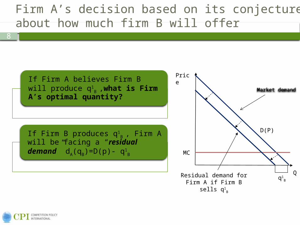
Firm A’s decision based on its conjecture about how much firm B will offer
If Firm A believes Firm B will produce q1
B ,what is Firm A’s optimal quantity?
If Firm B produces q1B , Firm A will
be facing a “residual demand” dA(qB)=D(p)- q1
B
Market demand
Residual demand for Firm A if Firm B sells q1
B
Price
D(P)
Q
MC
q1B
9
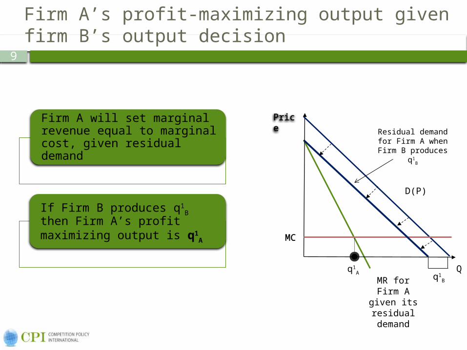
Firm A’s profit-maximizing output given firm B’s output decision
Firm A will set marginal revenue equal to marginal cost, given residual demand
If Firm B produces q1B then Firm A’s profit maximizing output is q1A
Price
MC
Residual demand for Firm A when Firm B
produces q1B
MR for Firm A given its
residual demand
q1A
Price
D(P)
Q
MC
q1B

10
Firm A’s decision on how much to supply varies with its conjecture about firm B’s supply
Note that when qB=0, the residual demand for Firm A equals the market demand
Hence, the optimal quantity chosen by Firm A is that of a monopolist: qM
A
Price
Q
MC
q1B
D(P)
Residual demand for Firm A when Firm B
produces q1B
MR for Firm A given its residual
demand
q1A

11
The “best response curve” summarizes A’s best moves for each of B’s choices
For each value of qB, Firm A has a Best Response based on its maximizing profits rule.
We can write down a schedule of these “best responses” for Firm A for every possible output by Firm B. This is called Firm A’s “Reaction Function” or “Best Response Function”.
The reaction function is key for analyzing the equilibrium decisions of oligopoly firms.
12
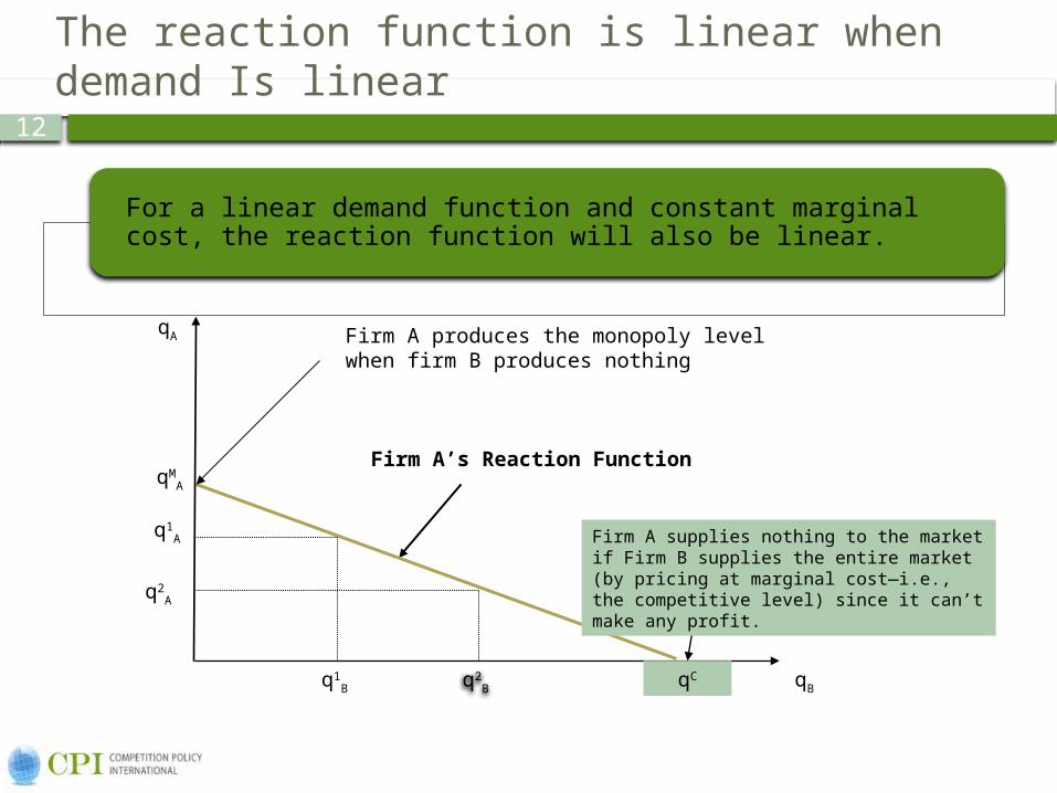
The reaction function is linear when demand Is linear
For a linear demand function and constant marginal cost, the reaction function will also be linear.
q2Bq1
B qB
Firm A’s Reaction Function
qC
qMA
qA
q2A
q1A
Firm A produces the monopoly level when firm B produces nothing
Firm A supplies nothing to the market if Firm B supplies the entire market (by pricing at marginal cost—i.e., the competitive level) since it can’t make any profit.
13
Firm B also has a reaction function based on a similar analysis
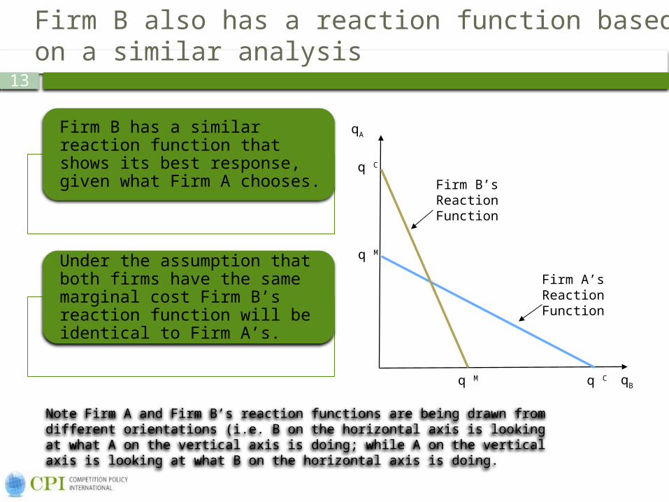
Firm B has a similar reaction function that shows its best response, given what Firm A chooses.
Under the assumption that both firms have the same marginal cost Firm B’s reaction function will be identical to Firm A’s.
Note Firm A and Firm B’s reaction functions are being drawn from different orientations (i.e. B on the horizontal axis is looking at what A on the vertical axis is doing; while A on the vertical axis is looking at what B on the horizontal axis is doing.
qA
Firm A’s Reaction Function
q C
q M
q M
q C
Firm B’s Reaction Function
qB
14
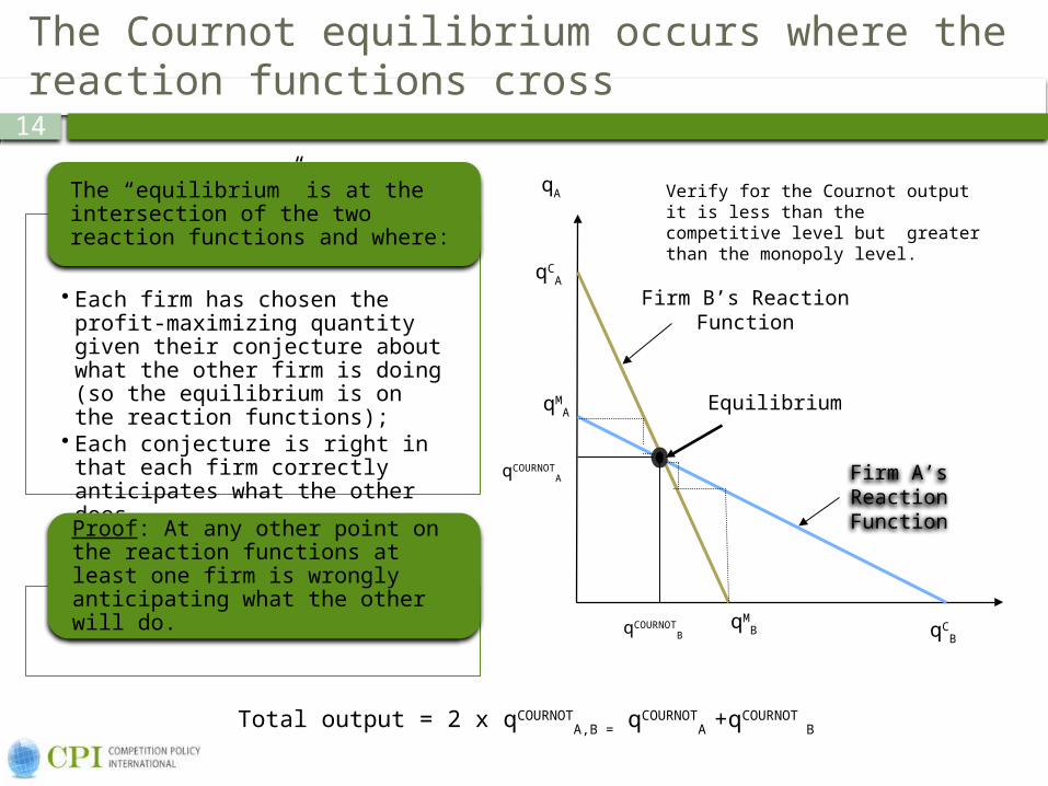
The Cournot equilibrium occurs where the reaction functions cross
• Each firm has chosen the profit-maximizing quantity given their conjecture about what the other firm is doing (so the equilibrium is on the reaction functions);
• Each conjecture is right in that each firm correctly anticipates what the other does.
The “equilibrium” is at the intersection of the two reaction functions and where:
Proof: At any other point on the reaction functions at least one firm is wrongly anticipating what the other will do.
Firm A’s Reaction Function
qCB
qMA
qMB
Firm B’s Reaction Function
Equilibrium
qCOURNOTB
qA Verify for the Cournot output it is less than the competitive level but greater than the monopoly level.
qCA
qCOURNOTA
Total output = 2 x qCOURNOTA,B = qCOURNOT
A +qCOURNOT B

15
With Cournot oligopoly, total price is more than with competition but less than with monopoly
In Cournot equilibrium, market price is lower than what a monopolist would charge but higher than the competitive one.
Deadweight loss is also lower than that in the monopoly case in the same market, but still positive.
qC
D(P)
COMPETITION
COURNOT
MONOPOLY
QQ COURNOTqMA,B
MC
P
PM
PCOURNOT

16
Introduction to the Bertrand model
Forty-five years after the publication of Cournot’s book, Joseph Bertrand (1874-1900) observed that Cournot’s results depended on the assumption that firms compete over quantities. [ See Bertrand, J. "Theorie Mathematique de la Richesse Sociale," Journal des Savants, 67, 1883, pp. 499-508]
Bertrand considers what happens if the firms’ “strategic variable” consists of prices instead of quantities. (Do you think firms are more likely to play price or quantity; does it depend on the features of the industry?)
Bertrand’s model adopts the same assumptions as Cournot theory except the strategic variable is price instead of quantity.

17
Firm A’s decision based on its conjecture about firm B’s price
Products are perfect substitutes: Whichever firm charges the lowest price gets all the sales.
If price set by Firm A (PA) is lower than price set by Firm B (PB), Firm A’s demand will be D(PA)—the market demand—whereas Firm B’s demand will be zero. And vice versa.
If both Firms set the same price P= PA= PB then each Firm will get half of the demand: ½ D(P) (assumes customers choose randomly since firms are identical).
D(P)PA
QA =D(PA < PB) Q
PB
Firm B charges a higher price but gets
zero demandP

18
The Best Strategy with Bertrand Competition
If Firm A conjectures Firm B will set monopoly price its best price is slightly below that then, it gets all the monopoly profits for itself.
If Firm A conjectures that Firm B will set price between competitive and monopoly price, its best price is again slightly below It doesn’t get all the monopoly profits but at least it gets all the profits available at this supra-competitive price.
If Firm A conjectures that Firm B will set price at competitive level its best price is also at the competitive level (equal to marginal cost) It loses money at a lower price and makes no sales at a higher price.
Firm B is symmetric to Firm A and behaves exactly in the same way.

19
Equilibrium with Bertrand competition
The equilibrium is where price equals marginal cost (the competitive level).
At any higher price the conjectures are inconsistent. Whatever price a firm expects, the other one will undercut it to get the whole market and the entire profits.
At the competitive price firms cannot cut prices any more because they will lose money (does predatory pricing make sense here?). And they cannot raise prices either because they will lose all sales.
So at P = MC conjectures are consistent with each other: if Firm A charges the competitive price, Firm B will too, and vice versa.
20
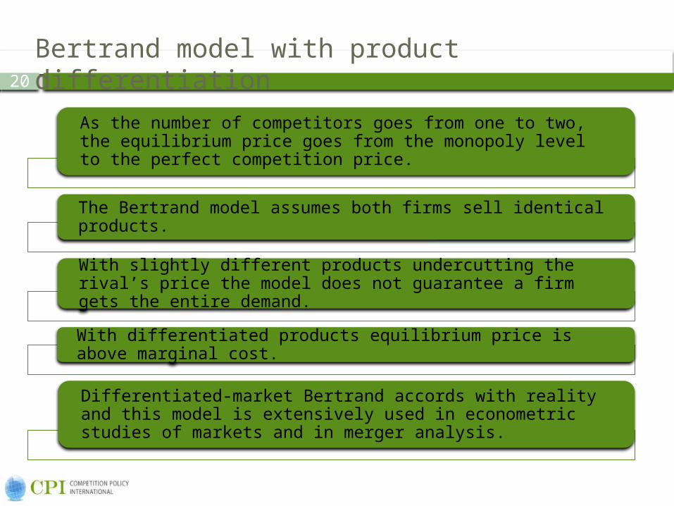
Bertrand model with product differentiation
As the number of competitors goes from one to two, the equilibrium price goes from the monopoly level to the perfect competition price.
The Bertrand model assumes both firms sell identical products.
With slightly different products undercutting the rival’s price the model does not guarantee a firm gets the entire demand.
With differentiated products equilibrium price is above marginal cost.
Differentiated-market Bertrand accords with reality and this model is extensively used in econometric studies of markets and in merger analysis.
21
Cournot and Bertrand can both be restated as games
The Cournot and Bertrand equilibria are Nash Equilibria in non-cooperative games.
Bertrand is an example of a prisoner’s dilemma game where the players independently choose the worst possible outcome.
Cournot is an example where the players in the end could have done better or could have done worse.
22
Oligopoly theory and the embarrassment of riches
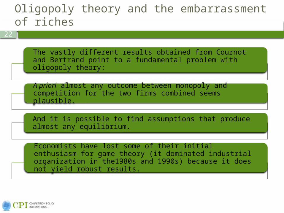
The vastly different results obtained from Cournot and Bertrand point to a fundamental problem with oligopoly theory:
A priori almost any outcome between monopoly and competition for the two firms combined seems plausible.
And it is possible to find assumptions that produce almost any equilibrium.
Economists have lost some of their initial enthusiasm for game theory (it dominated industrial organization in the1980s and 1990s) because it does not yield robust results.

23 Dynamic Games of Competition

24
Dynamic Games
Consider decision to enter and respond to entry:
Accomodate Fight
Enter (4,5) (-1,0)
Stay Out (0,10) (0,10)
Incumbent
Entrant
Entrant gets 4, Incumbent 5

25
Dynamic Equilibria and Credible Threats for the Entry Game
• Enter-Accommodate• Stay out-Fight
There are two possible equilibrium strategies:
• The incumbent can play its “fight” strategy and brag that it will demolish the entrant.
• But what if the entrant comes in (by mistake for example)?
• Once he is in, the incumbent is better off accommodating (is there an argument that it should fight nonetheless?)
• Key principle: threat must be credible to be effective.
But one of these isn’t credible:

26
Dynamic Games and Game Trees
Dynamic games are represented by game trees (“extensive form of a game”) that shows time-path of strategies:
Entrant
Incumbent
-1
0
4
5
0
10
EnterStay out
AccommodateFight

27
Solving the Game: Backward Induction
Start with what is optimal in the “end game” and then figure out what the optimal strategy is in the previous sub-games (this is known as “backward induction”—a very powerful technique in dynamic optimization theory).
Each player plays its best strategy in the sub-game knowing what has gone on before. This is known as the sub-game perfect Nash equilibrium.
28
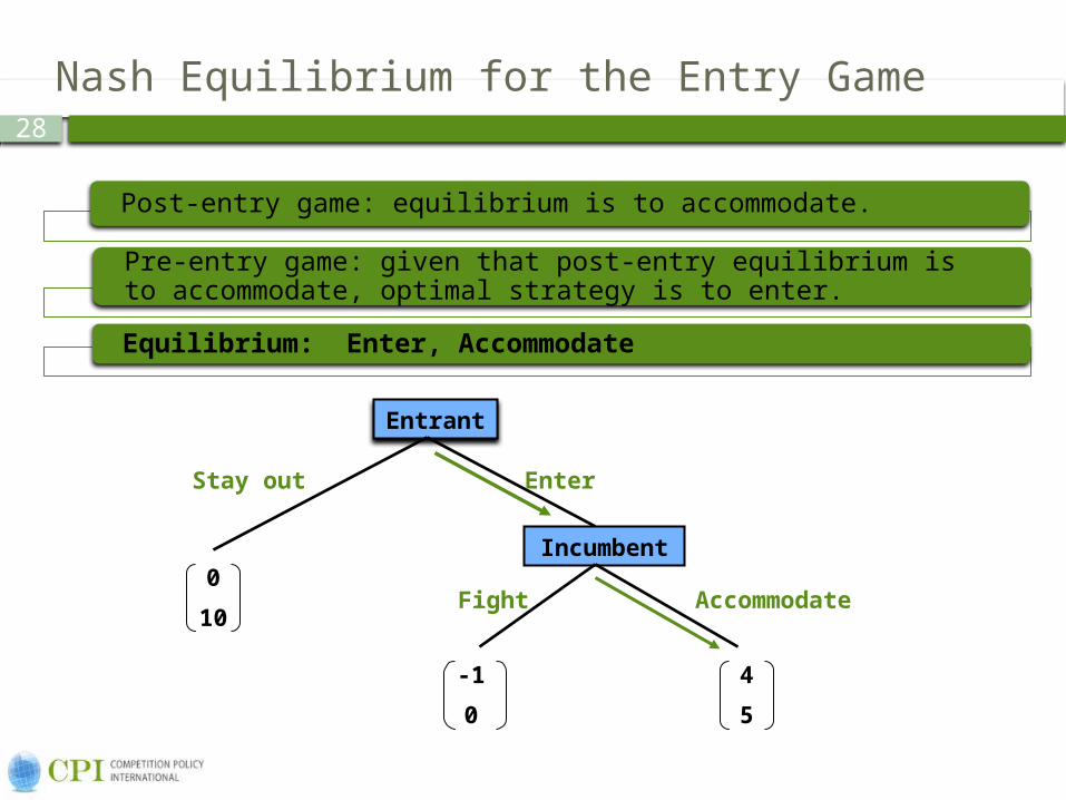
Nash Equilibrium for the Entry Game
Post-entry game: equilibrium is to accommodate.
Pre-entry game: given that post-entry equilibrium is to accommodate, optimal strategy is to enter.
Equilibrium: Enter, Accommodate
Entrant
Incumbent
-1
0
4
5
0
10
EnterStay out
AccommodateFight

29
Making Credible Commitments
Strategy analysis often considers whether players can make binding commitments that force them to undertake strategies that are ex post unprofitable but ex ante optimal.
For the entry game the incumbent could have “meeting competition clauses” or advertise “Our prices can’t be beat. We won’t be undersold.”
30
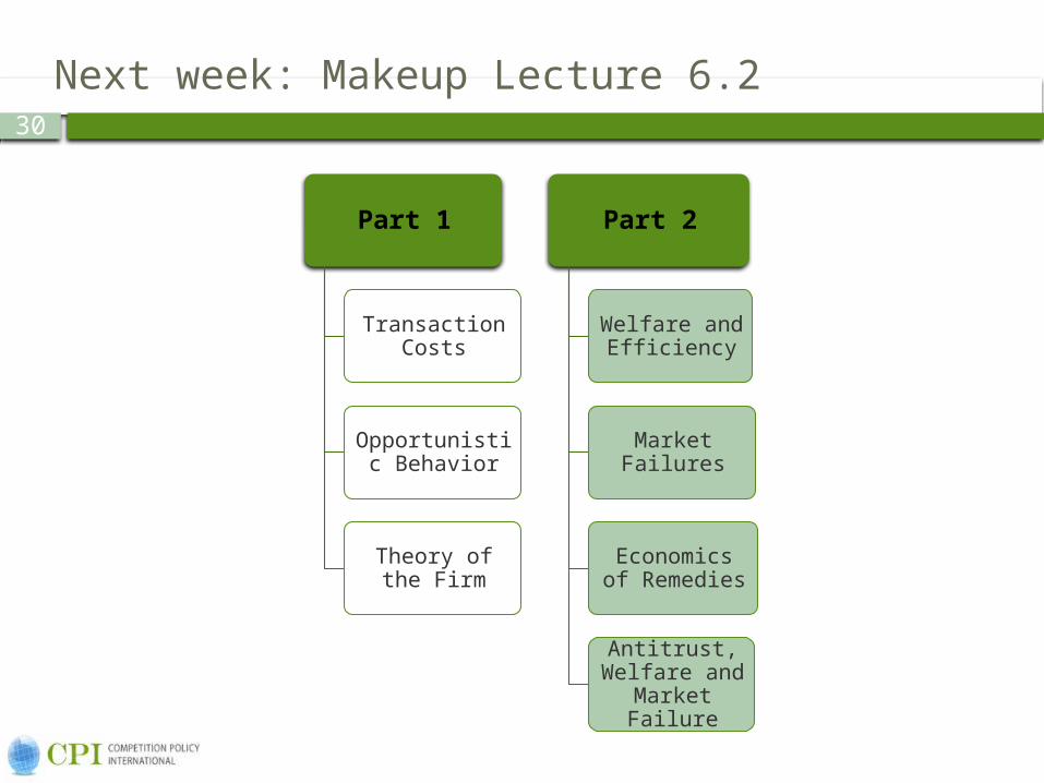
Next week: Makeup Lecture 6.2
Part 1
Transaction Costs
Opportunistic Behavior
Theory of the Firm
Part 2
Welfare and Efficiency
Market Failures
Economics of Remedies
Antitrust, Welfare and
Market Failure
Related Documents