Topic 7 Estimation Mathematics & Statistics Statistics.

Topic 7

Estimation

Mathematics & Statistics Statistics

Topic GoalsAfter completing this topic, you should be able

to: Distinguish between a point estimate and a

confidence interval estimate Construct and interpret a confidence interval

estimate for a single population mean using both the Z and t distributions

Form and interpret a confidence interval estimate for a single population proportion

Form and interpret a confidence interval estimate for a single population variance

Estimation

Last week we looked at the distribution of sample statistics...

...given the value of a population parameter. In real-life situations we don’t know the true value

of the population parameter... ...so the question is: Can we say something about the value of the

population parameter... ...given an observed value of a sample statistic?

Confidence Intervals

Content of this topic Confidence Intervals for the Population

Mean, μ when Population Variance σ2 is Known (Section 8.2) when Population Variance σ2 is Unknown (Section 8.3)

Confidence Intervals for the Population Proportion, p (large samples) (Section 8.4)

Confidence Intervals for the Population Variance, σ2 (Section 9.4)

Definitions

An estimator of a population parameter is a random variable that depends on sample

information . . . whose value provides an approximation to this

unknown parameter

A specific value of that random variable is called an estimate

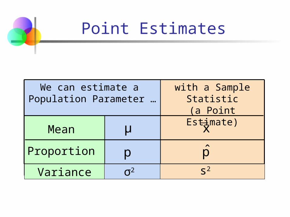
We can estimate a Population Parameter …

Point Estimates

with a SampleStatistic

(a Point Estimate)

Mean

Proportion p

xμ

p̂VarianceVariance σ2 s2

Unbiasedness

A point estimator is said to be an

unbiased estimator of the parameter if the

expected value, or mean, of the sampling

distribution of is ,

Examples: The sample mean is an unbiased estimator of μ The sample variance is an unbiased estimator of σ2

The sample proportion is an unbiased estimator of p

θ̂

θ̂

θ)θE( ˆ

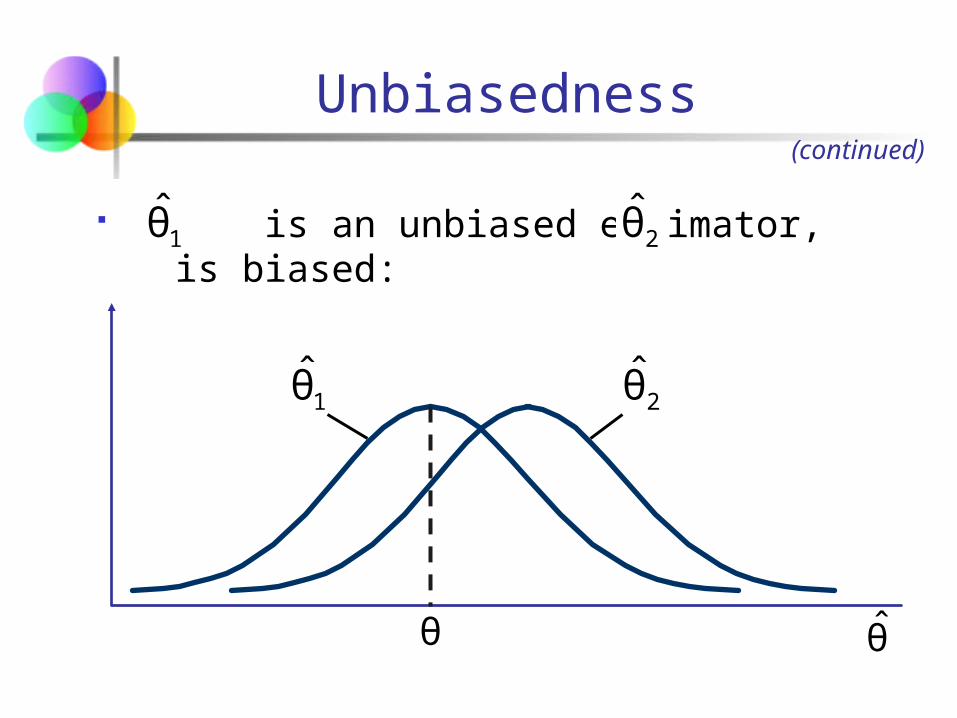
is an unbiased estimator, is biased:

1θ̂ 2θ̂

θ̂θ

1θ̂ 2θ̂

Unbiasedness(continued)

Most Efficient Estimator

Suppose there are several unbiased estimators of The most efficient estimator or the minimum variance

unbiased estimator of is the unbiased estimator with the smallest variance

Let and be two unbiased estimators of , based on the same number of sample observations. Then,

is said to be more efficient than if

The relative efficiency of with respect to is the ratio of their variances:

)θVar()θVar( 21ˆˆ

)θVar(

)θVar( Efficiency Relative

1

2

ˆ

ˆ

1θ̂ 2θ̂

1θ̂ 2θ̂

1θ̂ 2θ̂

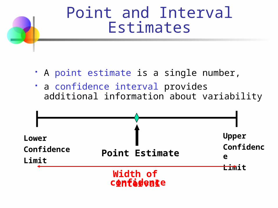
Point and Interval Estimates

A point estimate is a single number, a confidence interval provides additional

information about variability

Point Estimate

Lower

Confidence

Limit

Upper

Confidence

Limit

Width of confidence interval

Confidence Intervals

How much uncertainty is associated with a point estimate of a population parameter?

An interval estimate provides more information about a population characteristic than does a point estimate

Such interval estimates are called confidence intervals

Confidence Interval Estimate

An interval gives a range of values: Takes into consideration variation in sample

statistics from sample to sample Based on observation from 1 sample Gives information about closeness to

unknown population parameters Stated in terms of level of confidence

Can never be 100% confident

Confidence Interval and Confidence Level

If P(a < < b) = 1 - then the interval from a to b is called a 100(1 - )% confidence interval of .

The quantity (1 - ) is called the confidence level of the interval ( between 0 and 1)

In repeated samples of the population, the true value of the parameter would be contained in 100(1 - )% of intervals calculated this way.

The confidence interval calculated in this manner is written as a < < b with 100(1 - )% confidence

Estimation Process

(mean, μ, is unknown)

Population

Random Sample

Mean X = 50

Sample

I am 95% confident that μ is between 40 & 60.

Confidence Level, (1-)

Suppose confidence level = 95% Also written (1 - ) = 0.95 A relative frequency interpretation:

From repeated samples, 95% of all the confidence intervals that can be constructed will contain the unknown true parameter

A specific interval either will contain or will not contain the true parameter The procedure used leads to a correct interval in

95% of the time... ...but this does not guarantee anything about a

particular sample.

(continued)

General Formula

The general formula for all confidence intervals is:

The value of the reliability factor depends on the desired level of confidence

Point Estimate (Reliability Factor)(Standard deviation)

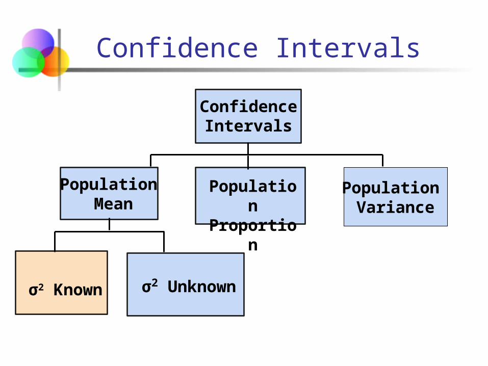
Confidence Intervals

Population Mean

σ2 Unknown

ConfidenceIntervals

PopulationProportion

σ2 Known

Population Variance

Confidence Interval for μ(σ2 Known)

Assumptions Population variance σ2 is known Population is normally distributed... ....or large sample so that CLT can be used.

Confidence interval estimate:

(where z/2 is the normal distribution value for a probability of /2 in each tail)

n

σzxμ

n

σzx α/2α/2

Example

A sample of 11 circuits from a large normal population has a mean resistance of 2.20 ohms. We know from past testing that the population standard deviation is 0.35 ohms.

Determine a 95% confidence interval for the true mean resistance of the population.

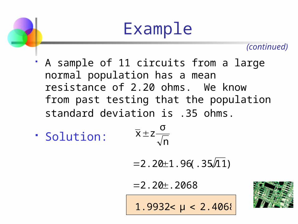
2.4068μ1.9932

.2068 2.20

)11(.35/ 1.96 2.20

n

σz x

Example

A sample of 11 circuits from a large normal population has a mean resistance of 2.20 ohms. We know from past testing that the population standard deviation is .35 ohms.

Solution:

(continued)

Interpretation

We are 95% confident that the true mean resistance is between 1.9932 and 2.4068 ohms

Although the true mean may or may not be in this interval, 95% of intervals formed in this manner will contain the true mean

Margin of Error

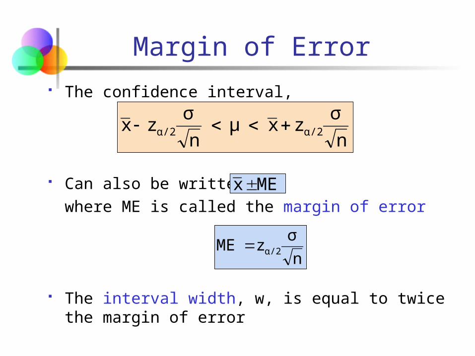
The confidence interval,

Can also be written as

where ME is called the margin of error

The interval width, w, is equal to twice the margin of error

n

σzxμ

n

σzx α/2α/2

MEx

n

σzME α/2

Finding the Reliability Factor, z/2

Consider a 95% confidence interval:

z = -1.96 z = 1.96

.951

.0252

α .025

2

α

Point EstimateLower Confidence Limit

UpperConfidence Limit

Z units:

X units:

0

Find z.025 = 1.96 from the standard normal distribution table

Common Levels of Confidence

Commonly used confidence levels are 90%, 95%, and 99%

Confidence Level

Confidence Coefficient,

Z/2 value

1.28

1.645

1.96

2.33

2.58

3.08

3.27

.80

.90

.95

.98

.99

.998

.999

80%

90%

95%

98%

99%

99.8%

99.9%

1

μμx

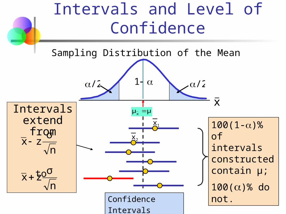
Intervals and Level of Confidence

Confidence Intervals

Intervals extend from

to

100(1-)%of intervals constructed contain μ;

100()% do not.

Sampling Distribution of the Mean

n

σzx

n

σzx

x

x1

x2

/2 /21

Summary:Finding a confidence interval for μ (σ known)

Choose confidence level 1-α (e.g. .95). Find an interval [a,b] such that P(a<μ<b)=1-α. a and b are determined by

How to find zα/2? Look in table for value such that P(Z> zα/2)=α

e.g. if 1-α=.95, then zα/2 = 1.96.

nzX

2/

Finding the Reliability Factor, z/2

Consider a 95% confidence interval:

z = -1.96 z = 1.96

.951

.0252

α .025

2

α

Point EstimateLower Confidence Limit

UpperConfidence Limit

Z units:

X units:

0

Find z.025 = 1.96 from the standard normal distribution table

Example

Assume that the calorie contents per 100 ml of Guiness is normally distributed.

A sample of 11 pints has a mean calorie content per 100 ml of 35.1. We know from past testing that the population standard deviation is 2.35.

Determine a 95% confidence interval for the true mean calorie content per 100 ml Guiness.

4888.63μ.711233

1.3888 .153

)11(2.35/ 1.96 1.53

n

σz x .05/2

Example

A sample of 11 pints from a large normal population has a mean calorie content per 100 ml of 35.1. We know from past testing that the population standard deviation is 2.35 calories per 100 ml.

Solution:

(continued)

Interpretation

We are 95% confident that the true calorie content per 100 ml is between 33.7112 and 36.4888.

Although the true mean may or may not be in this interval, 95% of intervals formed in this manner will contain the true mean

Example

Suppose a second sample of 11 pints has a mean calorie content per 100 ml of 35.9.

A 95% confidence interval for this sample is:

.288873μ.511243

1.3888 .953

)11(2.35/ 1.96 9.53

n

σz x .05/2

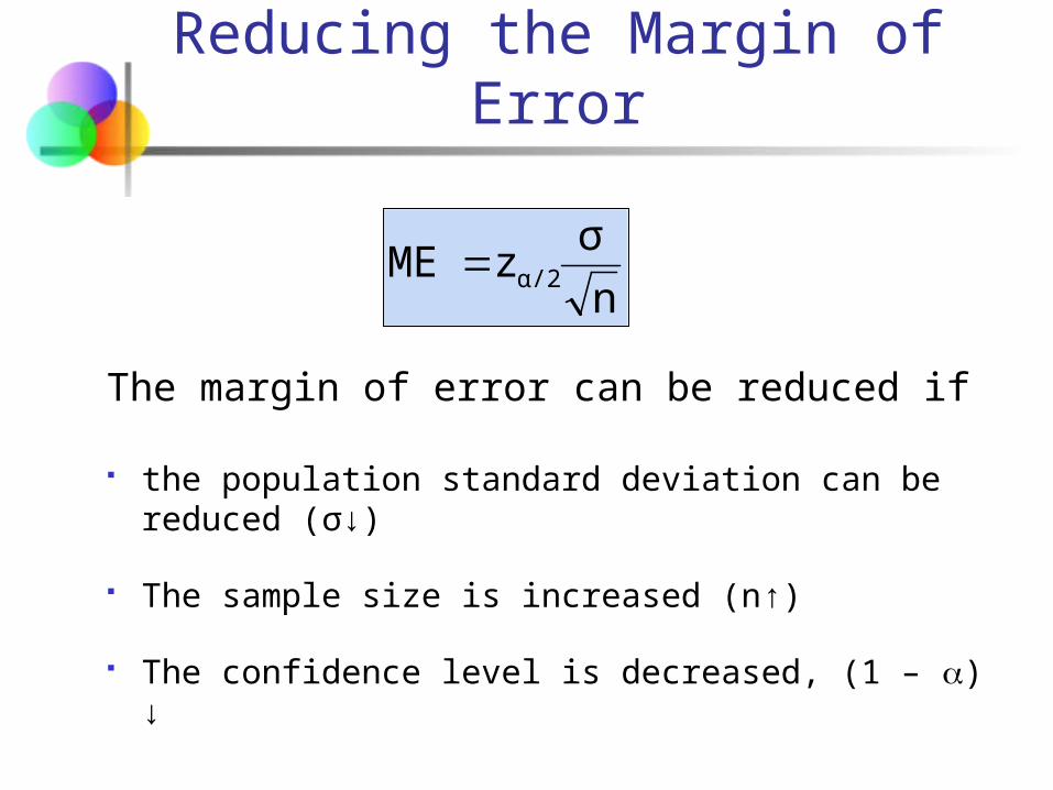
Reducing the Margin of Error

The margin of error can be reduced if

the population standard deviation can be reduced (σ↓)

The sample size is increased (n↑)

The confidence level is decreased, (1 – ) ↓

n

σzME α/2

How is the formula obtained?

Recall the formula for the confidence interval:

How is it obtained? A 100(1-α)% confidence interval is an interval [a,b] such

that P(a<μ<b) = 1-α. We use the fact that

n

σzxμ

n

σzx α/2α/2

)1,0(~/

Nn

XZ

Derivation

1)( 2/2/ zZzP

1

/2/2/ z

n

XzP

12/2/ zn

Xzn

P

12/2/ zn

Xzn

XP

12/2/ zn

Xzn

XP

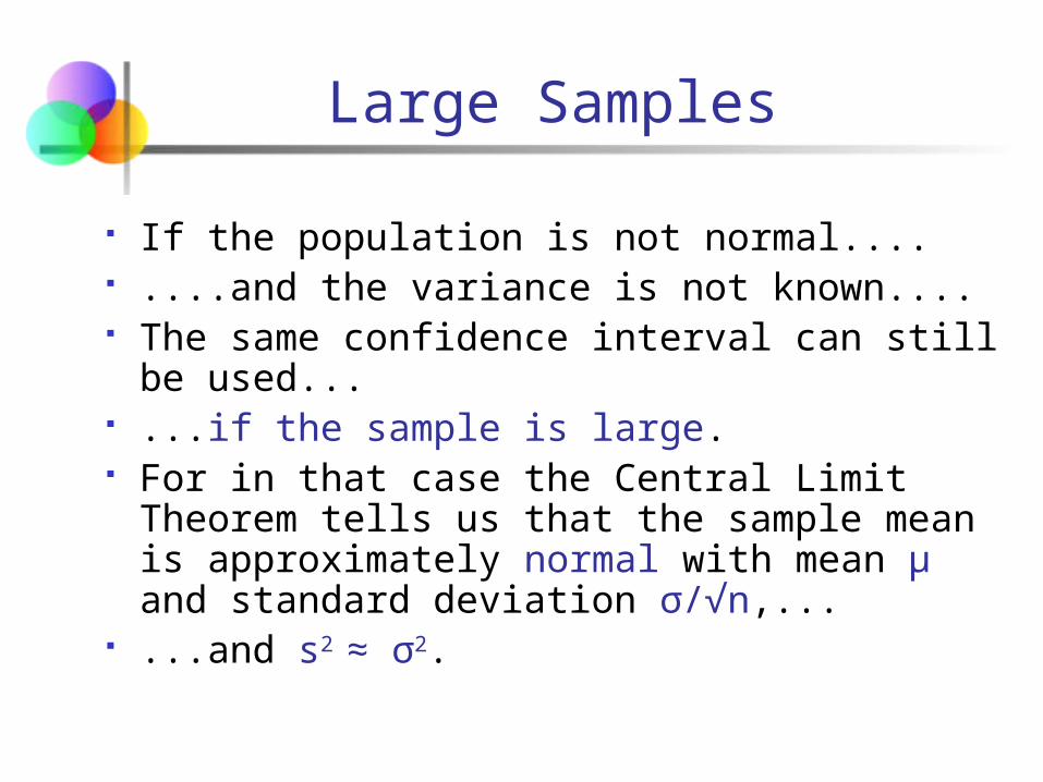
Large Samples

If the population is not normal.... ....and the variance is not known.... The same confidence interval can still be

used... ...if the sample is large. For in that case the Central Limit Theorem tells

us that the sample mean is approximately normal with mean μ and standard deviation σ/√n,...

...and s2 ≈ σ2.

Example

For a sample of 200 tea boxes you observe that the average weight is 101.0 grams with a standard deviation of 2.78 grams.

Determine a 99% confidence interval for the population mean.

Solution. Note that the sample is large, so: σ2 ≈ s2

the Central Limit Theorem says that the sample mean is approximately normal with mean μ and standard deviation σ/√n≈2.78/√200=.197

Example

So, we can proceed as if the sample mean is normal with known variance and apply

Therefore:

n

σzxμ

n

σzx α/2α/2

51.011μ49.001

.507 .0011

)200(2.78/ 2.58 .0011

n

σz x .01/2

Confidence Intervals

Population Mean

σ2 Unknown

ConfidenceIntervals

PopulationProportion

σ2 Known

Population Variance

If the population standard deviation σ is unknown, we can substitute the sample standard deviation, s

This introduces extra uncertainty, since s is variable from sample to sample

Therefore we use the t distribution instead of the normal distribution

Confidence Interval for μ(σ2 Unknown)

Student’s t Distribution

Consider a random sample of n observations with mean x and standard deviation s from a normally distributed population with mean μ

Then the variable

follows the Student’s t distribution with (n - 1) degrees of freedom

ns/

μxt

Student’s t Distribution

The t is a family of distributions

The t-value depends on degrees of freedom (d.f.) Number of observations that are free to vary after

sample mean has been calculated

d.f. = n - 1

Student’s t Distribution

t0

t (df = 5)

t (df = 13)t-distributions are bell-shaped and symmetric, but have ‘fatter’ tails than the normal

Standard Normal

(t with df = ∞)

Note: t Z as n increases

Assumptions Population standard deviation is unknown Population is normally distributed

Use Student’s t Distribution Confidence Interval Estimate:

where tn-1,α/2 is the critical value of the t distribution with n-1 d.f. and an area of α/2 in each tail:

Confidence Interval for μ(σ Unknown)

n

stxμ

n

stx α/21,-nα/21,-n

(continued)

α/2)tP(t α/21,n

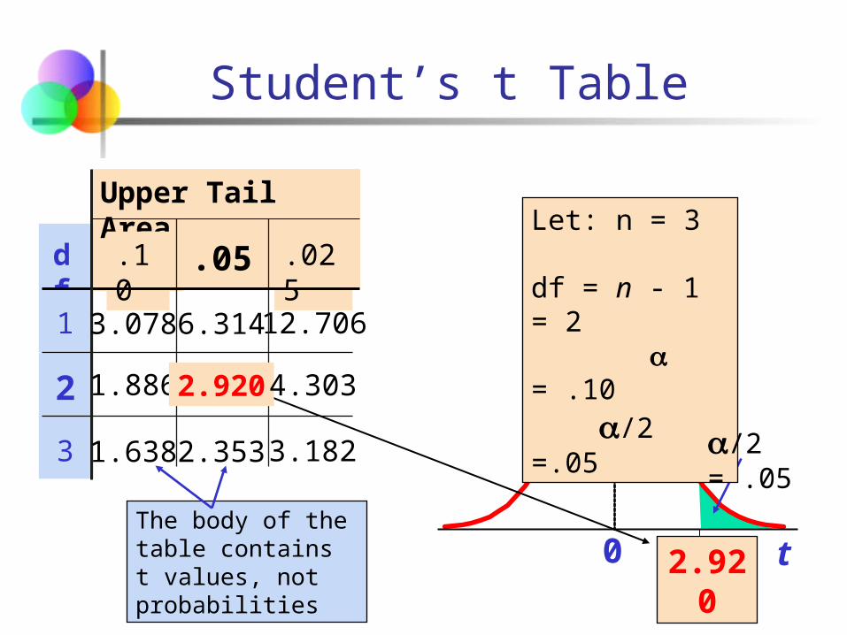
Student’s t Table

Upper Tail Area

df .10 .025.05

1 12.706

2

3 3.182

t0 2.920The body of the table contains t values, not probabilities

Let: n = 3 df = n - 1 = 2 = .10 /2 =.05

/2 = .05

3.078

1.886

1.638

6.314

2.920

2.353

4.303

t distribution values

With comparison to the Z value

Confidence t t t Z Level (10 d.f.) (20 d.f.) (30 d.f.) ____

.80 1.372 1.325 1.310 1.282

.90 1.812 1.725 1.697 1.645

.95 2.228 2.086 2.042 1.960

.99 3.169 2.845 2.750 2.576

Note: t Z as n increases

Example

A sample of 11 pints has a mean calorie content per 100 ml of 35.1, with a standard deviation of 2.35.

Determine a 95% confidence interval for the true mean calorie content per 100 ml Guiness if the calorie content is normal.

6787.63μ.521333

1.5787 .153

)11(2.35/ 2.228 1.53

n

s tx 10,.05/2

Example

A sample of 11 pints from a large normal population has a mean calorie content per 100 ml of 35.1, with a standard deviation of 2.35 calories per 100 ml.

Solution:

(continued)

Interpretation

We are 95% confident that the true calorie content per 100 ml is between 33.5213 and 36.6787.

Compare with the previous example (variance known)...

...where we were 95% confident that the true calorie content per 100 ml is between 33.7112 and 36.4888.

The interval is wider because there is additional uncertainty over σ.

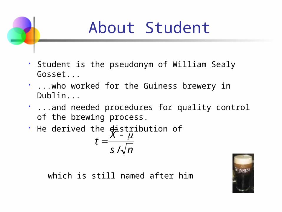
About Student

Student is the pseudonym of William Sealy Gosset... ...who worked for the Guiness brewery in Dublin... ...and needed procedures for quality control of the

brewing process. He derived the distribution of

which is still named after him

ns

Xt

/

Confidence Intervals

Population Mean

σ2 Unknown

ConfidenceIntervals

PopulationProportion

σ2 Known

Population Variance

Confidence Intervals for the Population Proportion, p

An interval estimate for the population proportion ( p ) can be calculated by adding an allowance for uncertainty to the sample proportion ( )

Sample has to be large because we will use the normal approximation to the binomial

p̂

Confidence Intervals for the Population Proportion, p

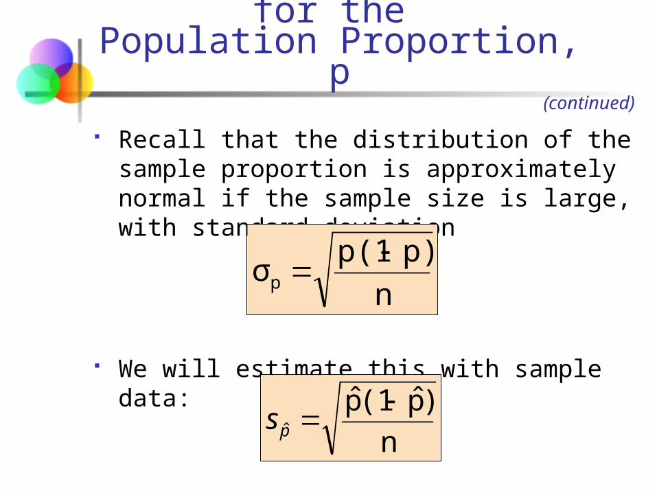
Recall that the distribution of the sample proportion is approximately normal if the sample size is large, with standard deviation

We will estimate this with sample data:

(continued)

n

)p̂(1p̂ˆ

ps

n

p)p(1σp

Confidence Interval Endpoints

Upper and lower confidence limits for the population proportion are calculated with the formula

where z/2 is the standard normal value for the level of confidence desired is the sample proportion n is the sample size

n

)p̂(1p̂zp̂p

n

)p̂(1p̂zp̂ α/2α/2

p̂

Example

A random sample of 100 people

shows that 25 are left-handed.

Form a 95% confidence interval for

the true proportion of left-handers

Example A random sample of 100 people shows

that 25 are left-handed. Form a 95% confidence interval for the true proportion of left-handers.

(continued)

0.3349p0.1651100

.25(.75)1.96

100

25p

100

.25(.75)1.96

100

25

n

)p̂(1p̂zp̂p

n

)p̂(1p̂zp̂ α/2α/2

Interpretation

We are 95% confident that the true percentage of left-handers in the population is between

16.51% and 33.49%.

Although the interval from 0.1651 to 0.3349 may or may not contain the true proportion, 95% of intervals formed from samples of size 100 in this manner will contain the true proportion.

General Example

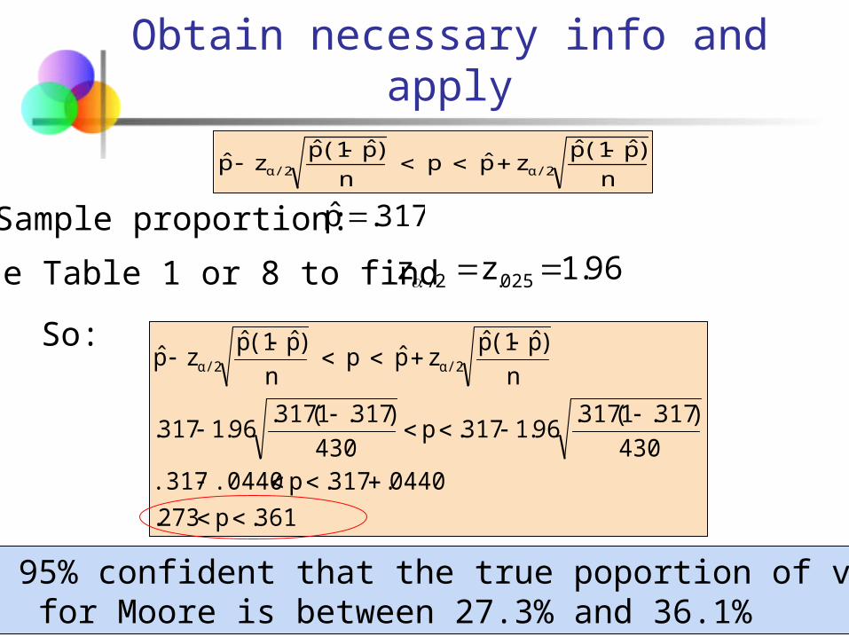
Trinity news, Issue 9, vol. 54 reports the results of a poll with 430 respondents on the SU president election. It is reported that: “Moore [has] the slightest lead of 31.7% to [...] Donohue’s 29.2% [...] and Reilly’s 27.2%. Given the margin of error the narrow gap [...] means any one [can win]”.

Compute a 95% confidence interval for the proportion of votes for Moore.

What do you think about the paper’s claim referring to the margin of error?

First question

We have a large sample: n = 430 We are asked to compute a 95% confidence level:

1-α=.95 and – thus – α=.05. The quantity of interest is a population proportion. Let p denote the proportion of votes for Moore. So, the appropriate confidence interval is

n

)p̂(1p̂zp̂p

n

)p̂(1p̂zp̂ α/2α/2

Obtain necessary info and apply

361.p273.

0440.317.p.0440 .317430

)317.1(317.96.1317.p

430

)317.1(317.96.1317.

n

)p̂(1p̂zp̂p

n

)p̂(1p̂zp̂ α/2α/2

317.p̂

96.1zz 025.2/

Sample proportion:

Use Table 1 or 8 to find

So:

We are 95% confident that the true poportion of votesfor Moore is between 27.3% and 36.1%

n

)p̂(1p̂zp̂p

n

)p̂(1p̂zp̂ α/2α/2

Second questionWe are 95% confident that the true poportion of votes

for Moore is between 27.3% and 36.1%

The score for Donohue is 29.2% and lies inside this95% confidence interval, Reilly’s 27.2%, however, does not. So, given the chosen level of confidence and the resulting margin of error, the race could be

deemed “too close to call” between Moore and Donohue.

NB The article does not specify the confidence level.So, we don’t know what “margin of error” it refers to.

Bad statistical practise.

Probability Question

In a particular city, 20% of mobile phones are owned by people younger than 15. In addition, 52% of people with a mobile phone have a “Pay As You Talk” deal. Among those younger than 15, 12% have a “Pay As You Talk” deal.

What is the probability that a randomly chosen mobile phone is “Pay As You Talk” and belongs to someone younger than 15?

Set up the analysis

Give the events of interest a name: Let A be the event that the phone belongs to a person

younger than 15. Let B be the event that the phone is “Pay As You Talk”

What probabilties are given? P(A) = .2 P(B) = .52 P(B|A) = .12

What are we asked? Joint probability of A and B: P(A∩B)

Find Solution

We know that:

Therefore,

)A(P

)BA(P)A|B(P

024.

2.*12.

)A(P)A|B(P)BA(P

Exam Tips

Move on to next question if stuck Method more important than outcome

don’t worry too much about rounding (not too many digits)

computation errors have minor penalty Write down all the steps you take

avoids mistakes I can’t give marks if it’s not clear what you’re doing

Before you answer a question think about your “plan of attack” before you start writing.

Be relaxed when you walk in (no cramming).