Topic 4. Introduction to Communication Systems Telecommunication Systems Fundamentals Telecommunication Systems Fundamentals Profs. Javier Ramos & Eduardo Morgado Academic year 2.013-2.014

Welcome message from author
This document is posted to help you gain knowledge. Please leave a comment to let me know what you think about it! Share it to your friends and learn new things together.
Transcript
Topic 4. Introduction to Communication Systems
Telecommunication Systems FundamentalsTelecommunication Systems Fundamentals
Profs. Javier Ramos & Eduardo MorgadoAcademic year 2.013-2.014

Concepts in this Chapter
• General Overview– Logarithmic Units (dB) and Link Budget– Review of fundamental parameters of physical layer: bandwidth, BER, SNR,
Rate…– Other merit figures: Quality of Service– A/D Converter– Circuit Commutation vs. Packet Commutation– Network Topologies
• Functional Block Diagram of Analog Communications link• Functional Block Diagram of a Digital Communications Link
– Block description– Digital Modulations– Multiplexing and Multiple Access
Telecommunication Systems Fundamentals
2
Theory classes: 3 sessions (6 hours)Problems resolution: 1 session (2 hours)Lab (Matlab): 2 hours
Bibliography
Communication Systems Engineering. John. G. Proakis. Prentice Hall
Sistemas de Comunicación. S. Haykin. Wiley
Digital Communications. Fundamentals and Applications. B. Digital Communications. Fundamentals and Applications. B. Sklar. Prentice Hall
Digital Communications. J. G. Proakis. McGraw-Hill
Communications Systems. A. Bruce Carlson y Paul B. Crilly. Mc Graw Hill
Telecommunication Systems Fundamentals
3

Logarithmic Units (dB)
• When measuring a physical magnitude, we have to provide two pieces of information: a quantity (typically a number either integer or real) and the units. For example, when measuring the diameter of a tennis ball, we provide de number 6 but also the units “cm” (centimeters). In this example, the measurement of the diameter of the tennis ball is 6 cm. If we change units the number of the measurement – the quantity – will also change. In our example the diameter ball may be 60 mm, or 0.00006 Km.
• Obviously the adequate selection of units helps the handling of measurements. In our example, to measure the tennis ball the unit “cm” seems to be adequate, but when measuring the Earth radius the unit “Km” seems to be more appropriate. when measuring the Earth radius the unit “Km” seems to be more appropriate. More extreme is the case of measuring the Sun radius. If we use the same units –meters – for the three measurements, we would get 0,06 m, 12.756.000 m and 1.392.000.000 m for the tennis ball, Earth and Sun respectively.
• Having so extreme differences on the measurements results in practical problems. For example, try to plot the three measurements in the same graph. If you take a scale to accommodate the Sun radius, the radios of the tennis ball will appear as negligible (cero), but it is not.
Telecommunication Systems Fundamentals
4
Logarithmic Units (dB)
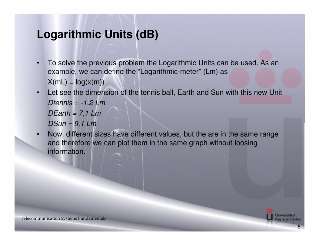
• To solve the previous problem the Logarithmic Units can be used. As an example, we can define the “Logarithmic-meter” (Lm) as
X(mL) = log(x(m))
• Let see the dimension of the tennis ball, Earth and Sun with this new Unit
Dtennis = -1,2 Lm
DEarth = 7,1 Lm
DSun = 9,1 LmDSun = 9,1 Lm
• Now, different sizes have different values, but the are in the same range and therefore we can plot them in the same graph without loosing information.
Telecommunication Systems Fundamentals
5
Logarithmic Units (dB)
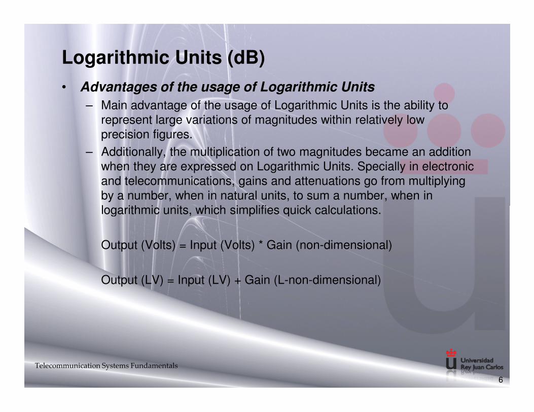
• Advantages of the usage of Logarithmic Units
– Main advantage of the usage of Logarithmic Units is the ability to represent large variations of magnitudes within relatively low precision figures.
– Additionally, the multiplication of two magnitudes became an addition when they are expressed on Logarithmic Units. Specially in electronic and telecommunications, gains and attenuations go from multiplying by a number, when in natural units, to sum a number, when in logarithmic units, which simplifies quick calculations. logarithmic units, which simplifies quick calculations.
Output (Volts) = Input (Volts) * Gain (non-dimensional)
Output (LV) = Input (LV) + Gain (L-non-dimensional)
Telecommunication Systems Fundamentals
6
Logarithmic Units (dB)
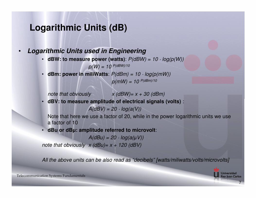
• Logarithmic Units used in Engineering• dBW: to measure power (watts): P(dBW) = 10 · log(p(W))
p(W) = 10 P(dBW)/10
• dBm: power in miliWatts: P(dBm) = 10 · log(p(mW))
p(mW) = 10 P(dBm)/10
note that obviously x (dBW)= x + 30 (dBm)
• dBV: to measure amplitude of electrical signals (volts) : • dBV: to measure amplitude of electrical signals (volts) :
A(dBV) = 20 · log(a(V))
Note that here we use a factor of 20, while in the power logarithmic units we use a factor of 10
• dBu or dBµ: amplitude referred to microvolt:
A(dBu) = 20 · log(a(µV))
note that obviously x (dBu)= x + 120 (dBV)
All the above units can be also read as “decibels” [watts/miliwatts/volts/microvolts]
Telecommunication Systems Fundamentals
7
Logarithmic Units (dB)
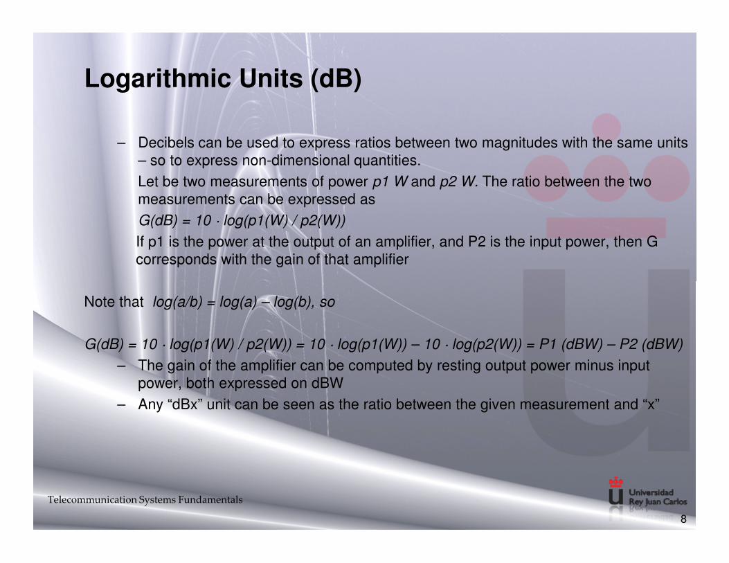
– Decibels can be used to express ratios between two magnitudes with the same units – so to express non-dimensional quantities.
Let be two measurements of power p1 W and p2 W. The ratio between the two measurements can be expressed as
G(dB) = 10 · log(p1(W) / p2(W))
If p1 is the power at the output of an amplifier, and P2 is the input power, then G corresponds with the gain of that amplifier
Note that log(a/b) = log(a) – log(b), so
G(dB) = 10 · log(p1(W) / p2(W)) = 10 · log(p1(W)) – 10 · log(p2(W)) = P1 (dBW) – P2 (dBW)
– The gain of the amplifier can be computed by resting output power minus input power, both expressed on dBW
– Any “dBx” unit can be seen as the ratio between the given measurement and “x”
Telecommunication Systems Fundamentals
8
Logarithmic Units (dB)
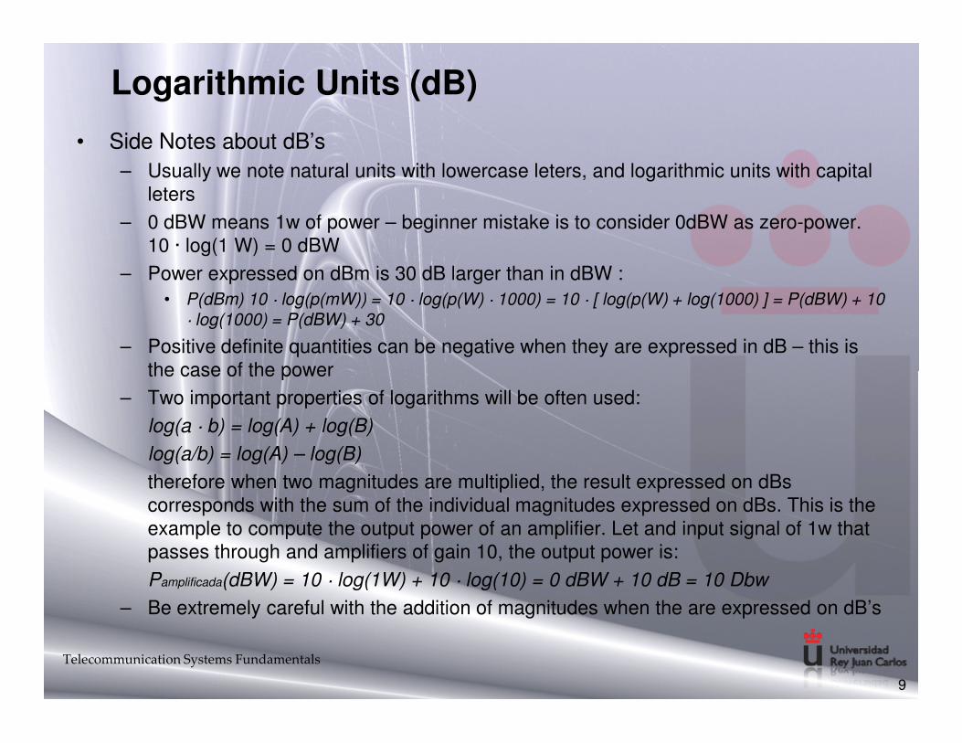
• Side Notes about dB’s
– Usually we note natural units with lowercase leters, and logarithmic units with capital leters
– 0 dBW means 1w of power – beginner mistake is to consider 0dBW as zero-power. 10 · log(1 W) = 0 dBW
– Power expressed on dBm is 30 dB larger than in dBW :
• P(dBm) 10 · log(p(mW)) = 10 · log(p(W) · 1000) = 10 · [ log(p(W) + log(1000) ] = P(dBW) + 10 · log(1000) = P(dBW) + 30
– Positive definite quantities can be negative when they are expressed in dB – this is the case of the powerthe case of the power
– Two important properties of logarithms will be often used:
log(a · b) = log(A) + log(B)
log(a/b) = log(A) – log(B)
therefore when two magnitudes are multiplied, the result expressed on dBscorresponds with the sum of the individual magnitudes expressed on dBs. This is the example to compute the output power of an amplifier. Let and input signal of 1w that passes through and amplifiers of gain 10, the output power is:
Pamplificada(dBW) = 10 · log(1W) + 10 · log(10) = 0 dBW + 10 dB = 10 Dbw
– Be extremely careful with the addition of magnitudes when the are expressed on dB’s
Telecommunication Systems Fundamentals
9
Logarithmic Units (dB)
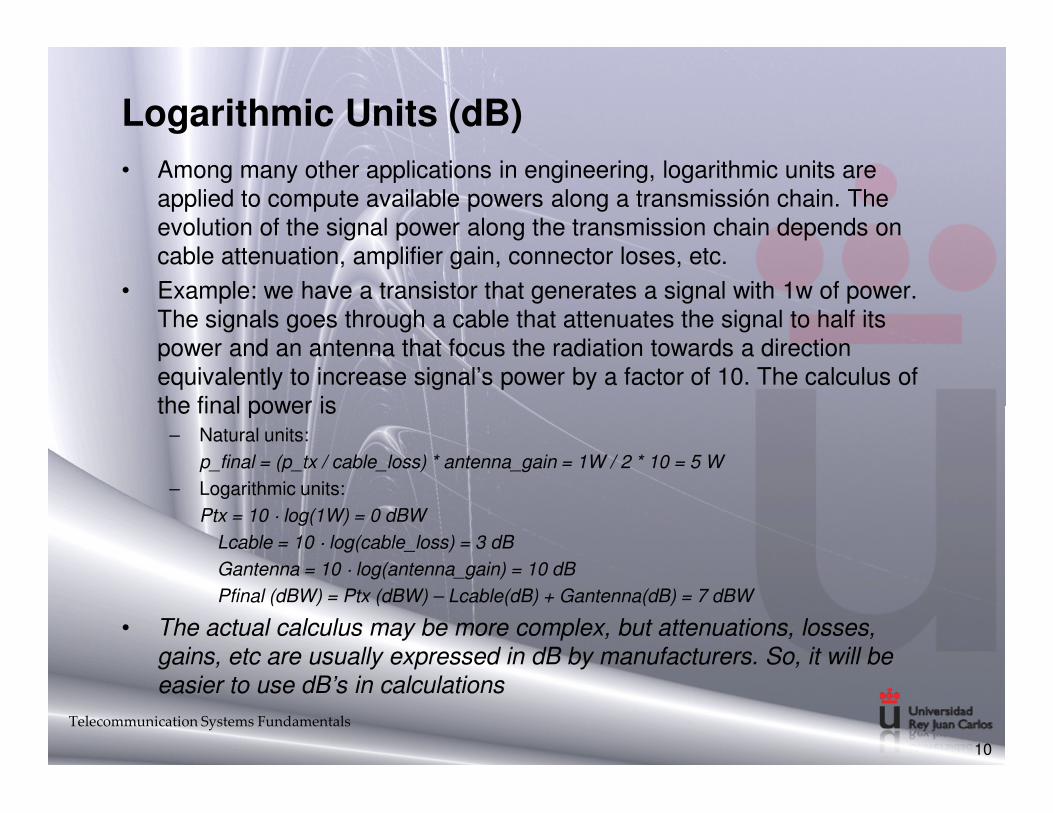
• Among many other applications in engineering, logarithmic units are applied to compute available powers along a transmissión chain. The evolution of the signal power along the transmission chain depends on cable attenuation, amplifier gain, connector loses, etc.
• Example: we have a transistor that generates a signal with 1w of power. The signals goes through a cable that attenuates the signal to half its power and an antenna that focus the radiation towards a direction equivalently to increase signal’s power by a factor of 10. The calculus of the final power isthe final power is
– Natural units:
p_final = (p_tx / cable_loss) * antenna_gain = 1W / 2 * 10 = 5 W
– Logarithmic units:
Ptx = 10 · log(1W) = 0 dBW
Lcable = 10 · log(cable_loss) = 3 dB
Gantenna = 10 · log(antenna_gain) = 10 dB
Pfinal (dBW) = Ptx (dBW) – Lcable(dB) + Gantenna(dB) = 7 dBW
• The actual calculus may be more complex, but attenuations, losses, gains, etc are usually expressed in dB by manufacturers. So, it will be easier to use dB’s in calculations
Telecommunication Systems Fundamentals
10

Concepts in this Chapter
• General Overview– Logarithmic Units (dB) and Link Budget– Review of fundamental parameters of physical layer: bandwidth, BER, SNR,
Rate…– Other merit figures: Quality of Service– A/D Converter– Circuit Commutation vs. Packet Commutation– Network Topologies
• Functional Block Diagram of Analog Communications link• Functional Block Diagram of a Digital Communications Link
– Block description– Digital Modulations– Multiplexing and Multiple Access
Telecommunication Systems Fundamentals
11
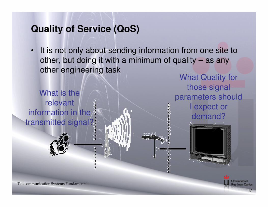
Quality of Service (QoS)
• It is not only about sending information from one site to other, but doing it with a minimum of quality – as any other engineering task
What is the relevant
What Quality for those signal
parameters should I expect or
Telecommunication Systems Fundamentals
12
relevant information in the
transmitted signal?
I expect or demand?
Quality of Service (QoS)
QoS defining parameters:
Telecommunication Systems Fundamentals
13
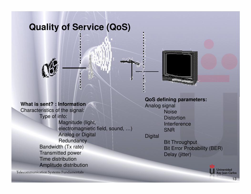
What is sent? : InformationCharacteristics of the signal:
Type of info:Magnitude (light, electromagnietic field, sound, …)Analog or DigitalRedundancy
Bandwidth (Tx rate)Transmitted powerTime distributionAmplitude distribution
QoS defining parameters:Analog signal
NoiseDistortionInterferenceSNR
DigitalBit ThroughputBit Error Probability (BER)Delay (jitter)
Quality of Service (QoS)
• Channel parameters that affect the QoS– Bandwidth
– Definition of Bandwidth for non-ideal channels (3dB, 90% of power, first null)
– Types of channel depending of its band-pass (low-pass, band-pass, high-pass, band-stopped)
– Attenuation (dB)
– Noise Figure– Noise Figure– Thermal noise
– Interferences
– Noise Equivalent Bandwidth
– Linear Distortion
• Amplitude and phase distortion
– Non-Linear Distortion
– Dynamic Range
Telecommunication Systems Fundamentals
14
Concepts in this Chapter
• General Overview– Logarithmic Units (dB) and Link Budget– Review of fundamental parameters of physical layer: bandwidth, BER, SNR,
Rate…– Other merit figures: Quality of Service– A/D Converter– Circuit Commutation vs. Packet Commutation– Network Topologies
• Functional Block Diagram of Analog Communications link• Functional Block Diagram of a Digital Communications Link
– Block description– Digital Modulations– Multiplexing and Multiple Access
Telecommunication Systems Fundamentals
15
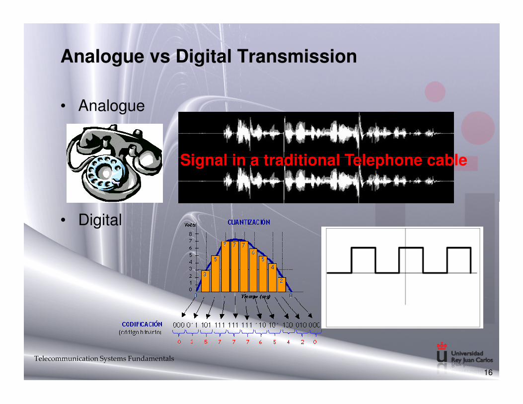
Analogue vs Digital Transmission
• Analogue
Signal in a traditional Telephone cable
• Digital
16
Telecommunication Systems Fundamentals
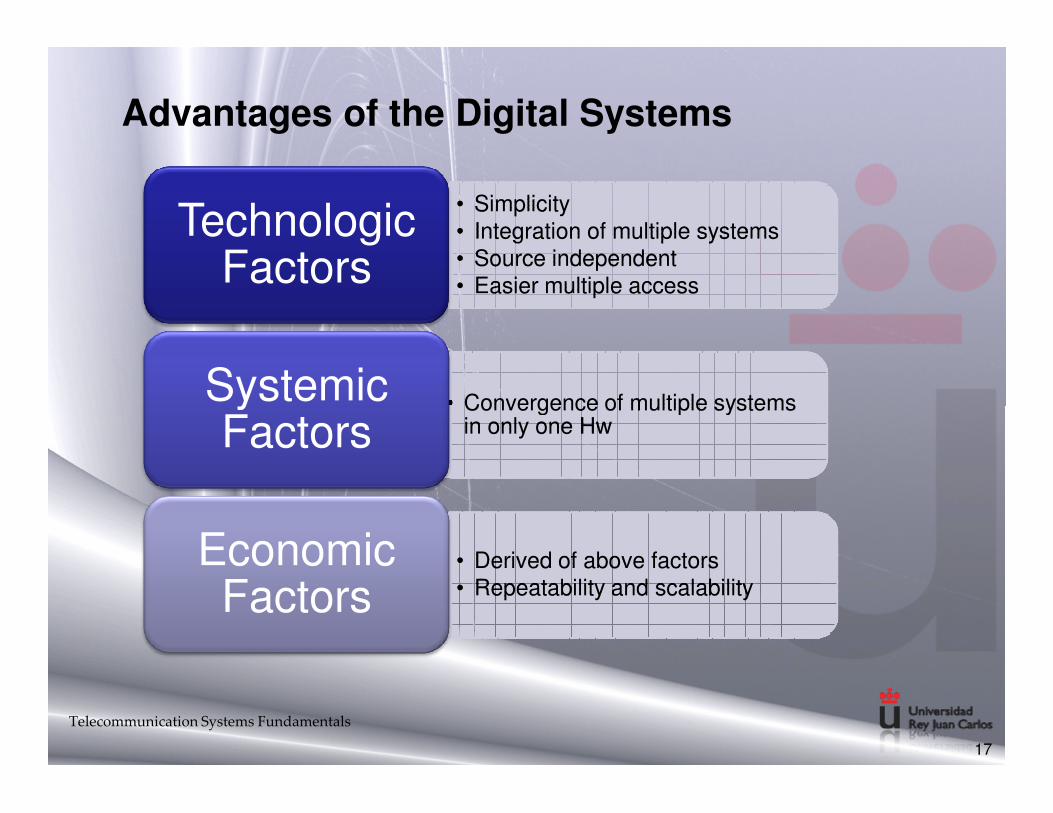
Advantages of the Digital Systems
• Simplicity• Integration of multiple systems• Source independent• Easier multiple access
• Simplicity• Integration of multiple systems• Source independent• Easier multiple access
Technologic Factors
• Convergence of multiple systems • Convergence of multiple systems Systemic
Telecommunication Systems Fundamentals
17
• Convergence of multiple systems in only one Hw
• Convergence of multiple systems in only one Hw
Systemic Factors
• Derived of above factors• Repeatability and scalability• Derived of above factors• Repeatability and scalability
Economic Factors
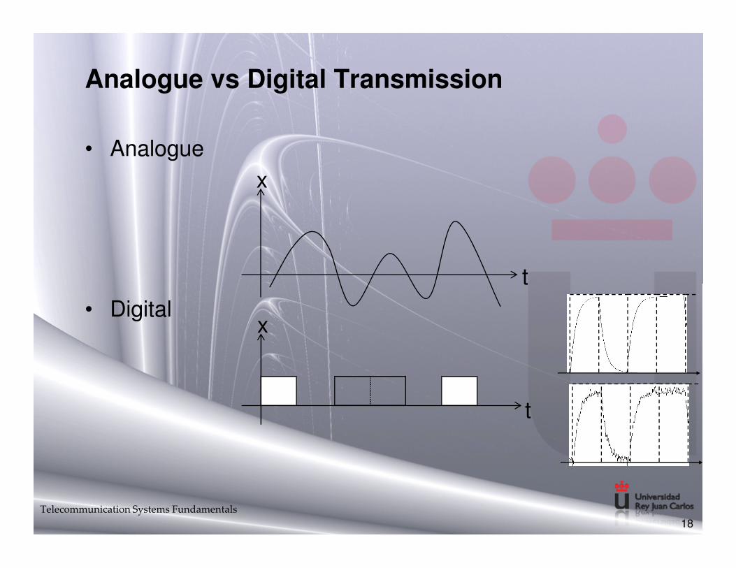
Analogue vs Digital Transmission
• Analogue
x
t
• Digital
18
Telecommunication Systems Fundamentals
x
t
t
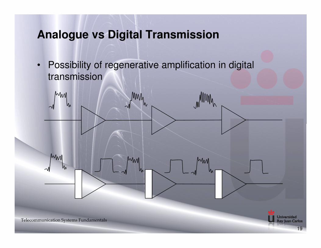
Analogue vs Digital Transmission
• Possibility of regenerative amplification in digital transmission
Telecommunication Systems Fundamentals
19
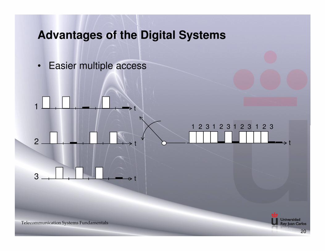
Advantages of the Digital Systems
• Easier multiple access
1
1 2 3 1 2 3 1 2 3 1 2 3
t
Telecommunication Systems Fundamentals
20
2
3
1 2 3 1 2 3 1 2 3 1 2 3
t
t
t

Analogue to Digital Conversión
• 3 Steps (first approach using traditional PCM – Pulse Coded Modulation:
– 1: Samplingx
t
– 2: Quantification
Telecommunication Systems Fundamentals
21
xq
x
xq

Analogue to Digital Conversión
– 3: Coding
x11100001
Telecommunication Systems Fundamentals
22
x
t
01
~

More Efficient Analogue to Digital Conversions
– Differential PCM
– Delta-Coding
– Sub-Bands Coding
– Compression and lossy coding
Telecommunication Systems Fundamentals
23

Concepts in this Chapter
• General Overview– Logarithmic Units (dB) and Link Budget– Review of fundamental parameters of physical layer: bandwidth, BER, SNR,
Rate…– Other merit figures: Quality of Service– A/D Converter– Circuit Commutation vs. Packet Commutation– Network Topologies
• Functional Block Diagram of Analog Communications link• Functional Block Diagram of a Digital Communications Link
– Block description– Digital Modulations– Multiplexing and Multiple Access
Telecommunication Systems Fundamentals
24
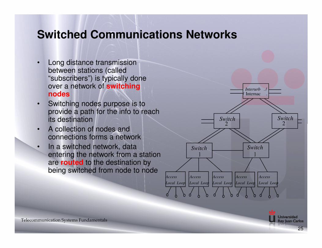
Switched Communications Networks
• Long distance transmission between stations (called “subscribers”) is typically done over a network of switchingnodes
• Switching nodes purpose is to provide a path for the info to reach its destination Switch
2
/.Interurb.Internac/
2Switch
• A collection of nodes and connections forms a network
• In a switched network, data entering the network from a station are routed to the destination by being switched from node to node
25
Telecommunication Systems Fundamentals
LoopLocal
Access
1
2 2
1Switch Switch
LoopLocal
Access
LoopLocal
Access
LoopLocal
Access
LoopLocal
Access
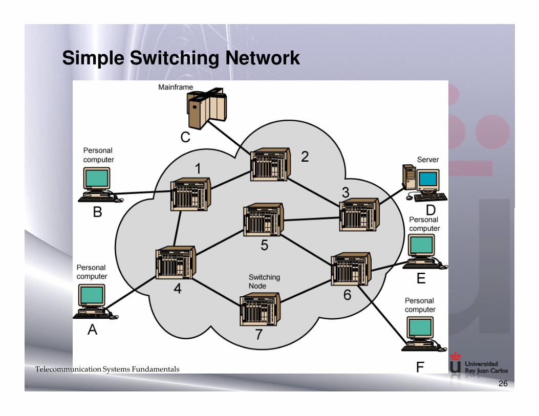
Simple Switching Network
26
Telecommunication Systems Fundamentals
Switching Nodes
• Nodes may connect to other nodes, or to some stations.
• Network is usually partially connected– However, some redundant connections are desirable for
reliability
• Two different switching technologies• Two different switching technologies– Circuit switching
– Packet switching
27
Telecommunication Systems Fundamentals

Circuit Switching
• Circuit switching:– There is a dedicated communication path between two subscribers
(end-to-end)
– The path is a connected sequence of links between network nodes. On each physical link, a logical channel is dedicated to the connection.
• Communication via circuit switching has three phases:– Circuit establishment (link by link)– Circuit establishment (link by link)
• Routing & resource allocation (FDM or TDM)
– Data transfer
– Circuit disconnect• Deallocate the dedicated resources
• The switches must know how to find the route to the destination and how to allocate bandwidth (channel) to establish a connection.
28
Telecommunication Systems Fundamentals
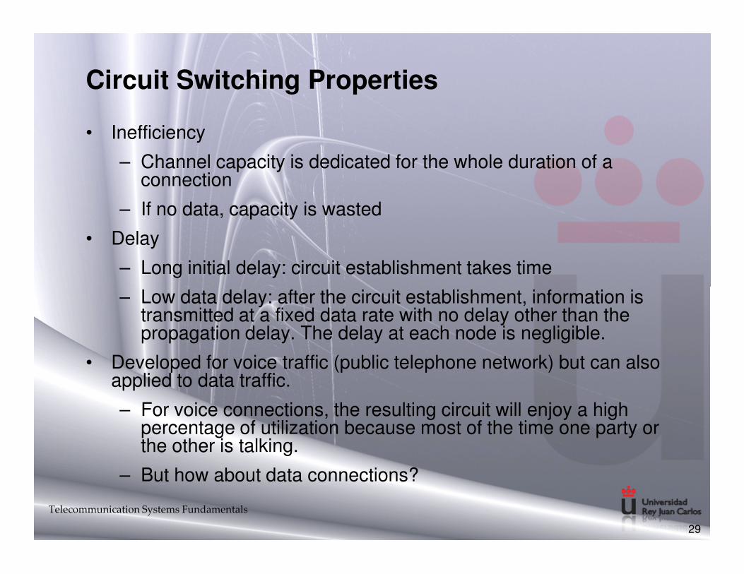
Circuit Switching Properties
• Inefficiency
– Channel capacity is dedicated for the whole duration of a connection
– If no data, capacity is wasted
• Delay
– Long initial delay: circuit establishment takes time
– Low data delay: after the circuit establishment, information is – Low data delay: after the circuit establishment, information is transmitted at a fixed data rate with no delay other than the propagation delay. The delay at each node is negligible.
• Developed for voice traffic (public telephone network) but can also applied to data traffic.
– For voice connections, the resulting circuit will enjoy a high percentage of utilization because most of the time one party or the other is talking.
– But how about data connections?
29
Telecommunication Systems Fundamentals
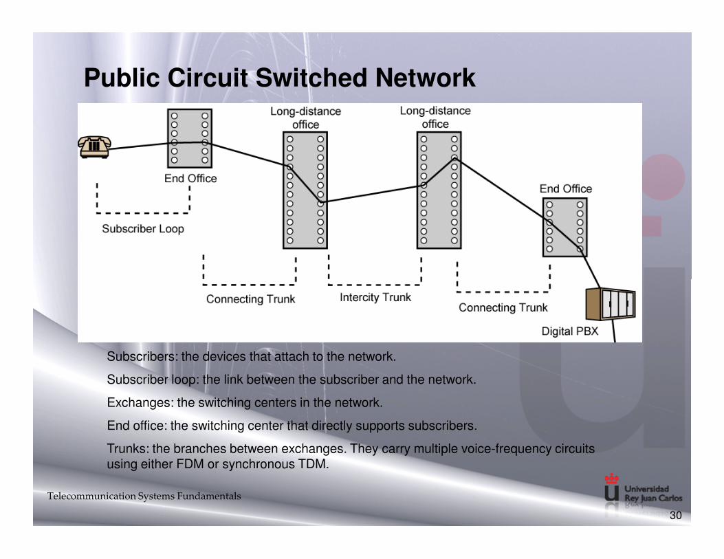
Public Circuit Switched Network
30
Subscribers: the devices that attach to the network.
Subscriber loop: the link between the subscriber and the network.
Exchanges: the switching centers in the network.
End office: the switching center that directly supports subscribers.
Trunks: the branches between exchanges. They carry multiple voice-frequency circuits using either FDM or synchronous TDM.
Telecommunication Systems Fundamentals

Packet Switching Principles
• Problem of circuit switching– Designed for voice service
– Resources dedicated to a particular call
– For data transmission, much of the time the connection is idle(say, web browsing)
– Data rate is fixed– Data rate is fixed
• Both ends must operate at the same rate during the entire period of connection
• Packet switching is designed to address these problems
31
Telecommunication Systems Fundamentals
Basic Operation
• Data are transmitted in short packets– Typically at the order of 1000 bytes
– Longer messages are split into series of packets
– Each packet contains a portion of user data plus some control info
• Control info contains at least• Control info contains at least– Routing (addressing) info, so as to be routed to the intended
destination
– Recall the content of an IP header!
• Store and Forward– On each switching node, packets are received, stored briefly
(buffered) and passed on to the next node.
32
Telecommunication Systems Fundamentals

Use of Packets
33
Telecommunication Systems Fundamentals

Advantages of Packet Switching
• Line efficiency
– Single node-to-node link can be dynamically shared by many packets over time
– Packets are queued up and transmitted as fast as possible
• Data rate conversion
– Each station connects to the local node at its own speed– Each station connects to the local node at its own speed
• In circuit-switching, a connection could be blocked if there lacks free resources. On a packet-switching network, even with heavy traffic, packets are still accepted, by delivery delay increases.
• Priorities can be used
– On each node, packets with higher priority can be forwarded first. They will experience less delay than lower-priority packets.
34
Telecommunication Systems Fundamentals
Packet Switching Technique
• A station breaks long message into packets
• Packets are sent out to the network sequentially, one at a time
• How will the network handle this stream of packets as it attempts to route them through the network and deliver them to the intended destination?deliver them to the intended destination?– Two approaches
• Datagram approach
• Virtual circuit approach
35
Telecommunication Systems Fundamentals

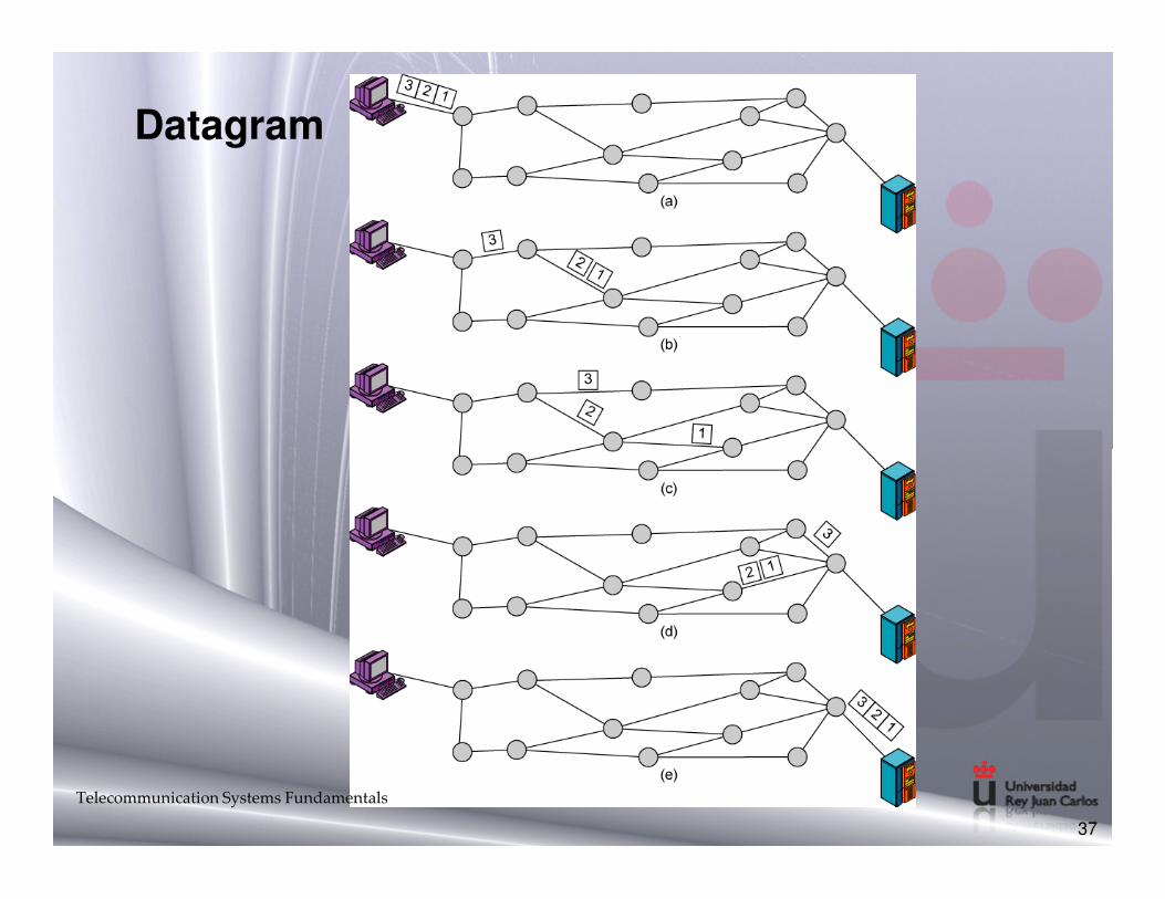
Datagram
• Each packet is treated independently, with no reference to packets that have gone before.
– Each node chooses the next node on a packet’s path
• Packets can take any possible route
• Packets may arrive at the receiver out of order
• Packets may go missing
• It is up to the receiver to re-order packets and recover from missing packets
• Example: Internet
36
Telecommunication Systems Fundamentals
Datagram
37
Telecommunication Systems Fundamentals
Virtual Circuit
• In virtual circuit, a preplanned route is established before any packets are sent, then all packets follow the same route
• Each packet contains a virtual circuit identifierinstead of destination address, and each node on the preestablished route knows where to forward such preestablished route knows where to forward such packets– The node need not make a routing decision for each packet
• Example: X.25, Frame Relay, ATM
38
Telecommunication Systems Fundamentals
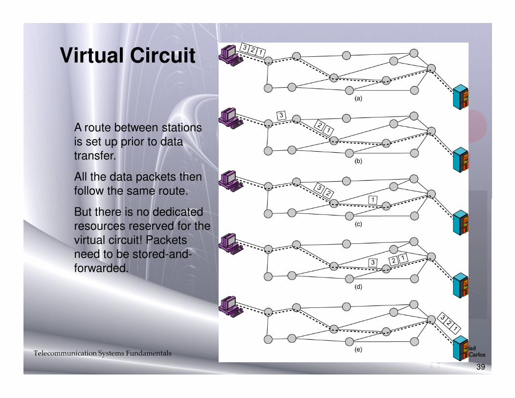
Virtual Circuit
A route between stations is set up prior to data transfer.
All the data packets then follow the same route.
39
But there is no dedicated resources reserved for the virtual circuit! Packets need to be stored-and-forwarded.
Telecommunication Systems Fundamentals
Virtual Circuits v Datagram
• Virtual circuits
– Network can provide sequencing (packets arrive at the same order) and error control (retransmission between two nodes).
– Packets are forwarded more quickly
• Based on the virtual circuit identifier
• No routing decisions to make
– Less reliable– Less reliable
• If a node fails, all virtual circuits that pass through that node fail
• Datagram
– No call setup phase
• Good for bursty data, such as Web applications
– More flexible
• If a node fails, packets may find an alternate route
• Routing can be used to avoid congested parts of the network
40
Telecommunication Systems Fundamentals

Concepts in this Chapter
• General Overview– Logarithmic Units (dB) and Link Budget– Review of fundamental parameters of physical layer: bandwidth, BER, SNR,
Rate…– Other merit figures: Quality of Service– A/D Converter– Circuit Commutation vs. Packet Commutation– Network Topologies
• Functional Block Diagram of Analog Communications link• Functional Block Diagram of a Digital Communications Link
– Block description– Digital Modulations– Multiplexing and Multiple Access
Telecommunication Systems Fundamentals
41
Theory classes: xx sessions (x hours)Problems resolution: 1 session (2 hours)Lab (Matlab): 2 hours
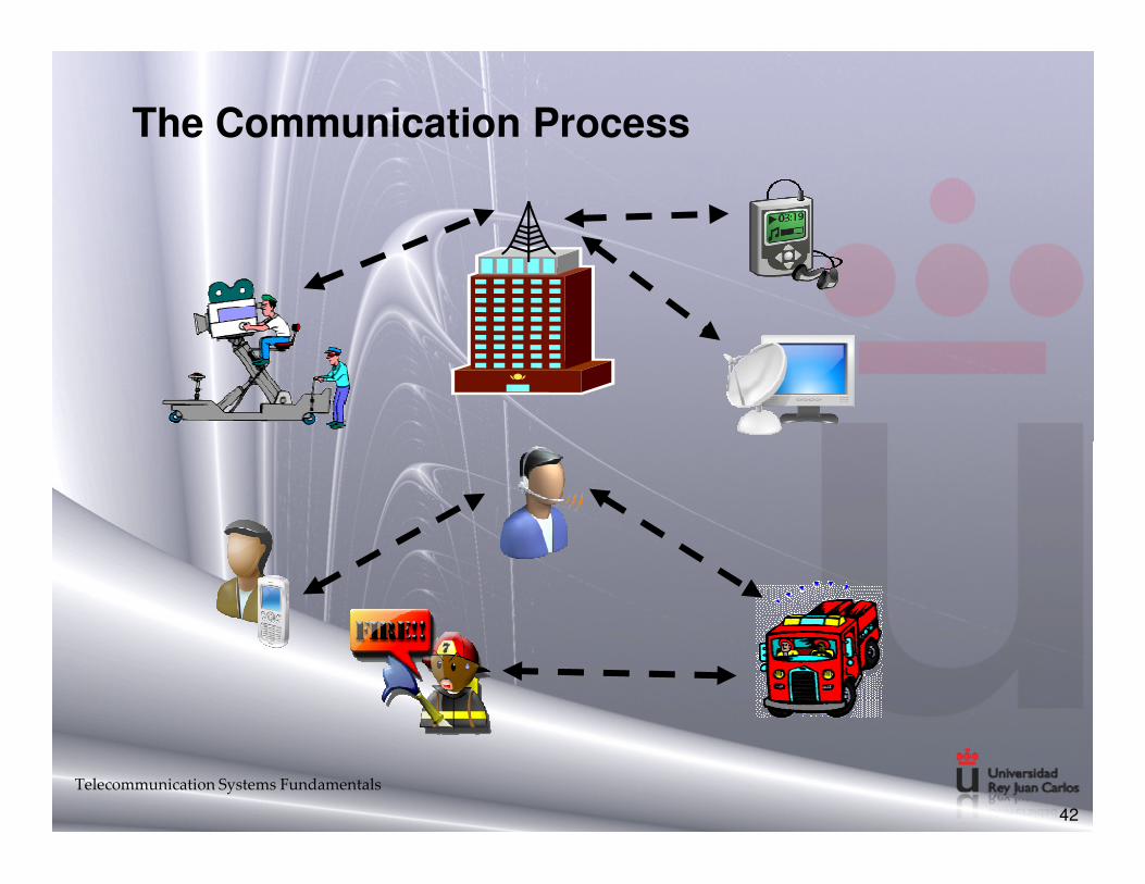
The Communication Process
Telecommunication Systems Fundamentals
42
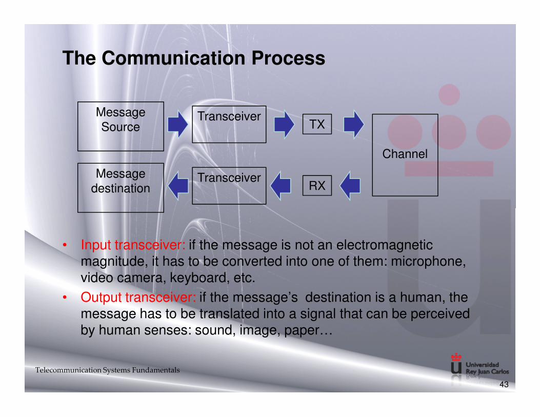
The Communication Process
TX
Channel
Message Source
Transceiver
RXMessage
destinationTransceiver
• Input transceiver: if the message is not an electromagnetic magnitude, it has to be converted into one of them: microphone, video camera, keyboard, etc.
• Output transceiver: if the message’s destination is a human, the message has to be translated into a signal that can be perceived by human senses: sound, image, paper…
Telecommunication Systems Fundamentals
43

The Layers of Communication
• What are the system requirements?• It has to be fast
• And ubiquitous (mobile)
• Secure
• Trustable (available)
• Cheap• Cheap
• User-friendly
• …
How can we cope with all specifications?
Telecommunication Systems Fundamentals
44

The Layers of Communication
• How can we design such a system?
Share the Channel
Access to the physical mean
Distinguish different sources
Enroute packets
Reduce the Cost
Telecommunication Systems Fundamentals
45
Find destination
Filter out noise
Reduce Tx power
Provide Security
and sessionsdifferent sources and sessions
Chop info into smaller pieces
Identify userRepair errors
Compress info
Systems are quite complex nowadays

The Layers of Communication: systems complexity
Telecommunication Systems Fundamentals
46

The Layers of Communication
• Solution: ¡Divide et Impera!
Telecommunication Systems Fundamentals
47
Mean Access
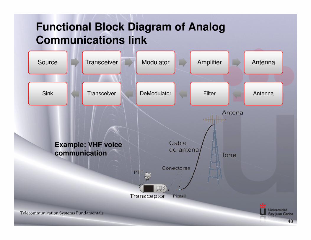
Functional Block Diagram of Analog Communications link
Source Transceiver Modulator Amplifier Antenna
Sink Transceiver DeModulator Filter Antenna
Telecommunication Systems Fundamentals
48
Example: VHF voice communication

Example: VHF voice communication
• Source: voice. Bandwidth: 3 KHz (to understand it) and 21 KHz (for HiFi)
• Transceiver: microphone. Piezoelectric device that translates mechanical pressure into voltage
• Modulator: change the central frequency of the signal spectrum to be transmitted through an antenna
Telecommunication Systems Fundamentals
49
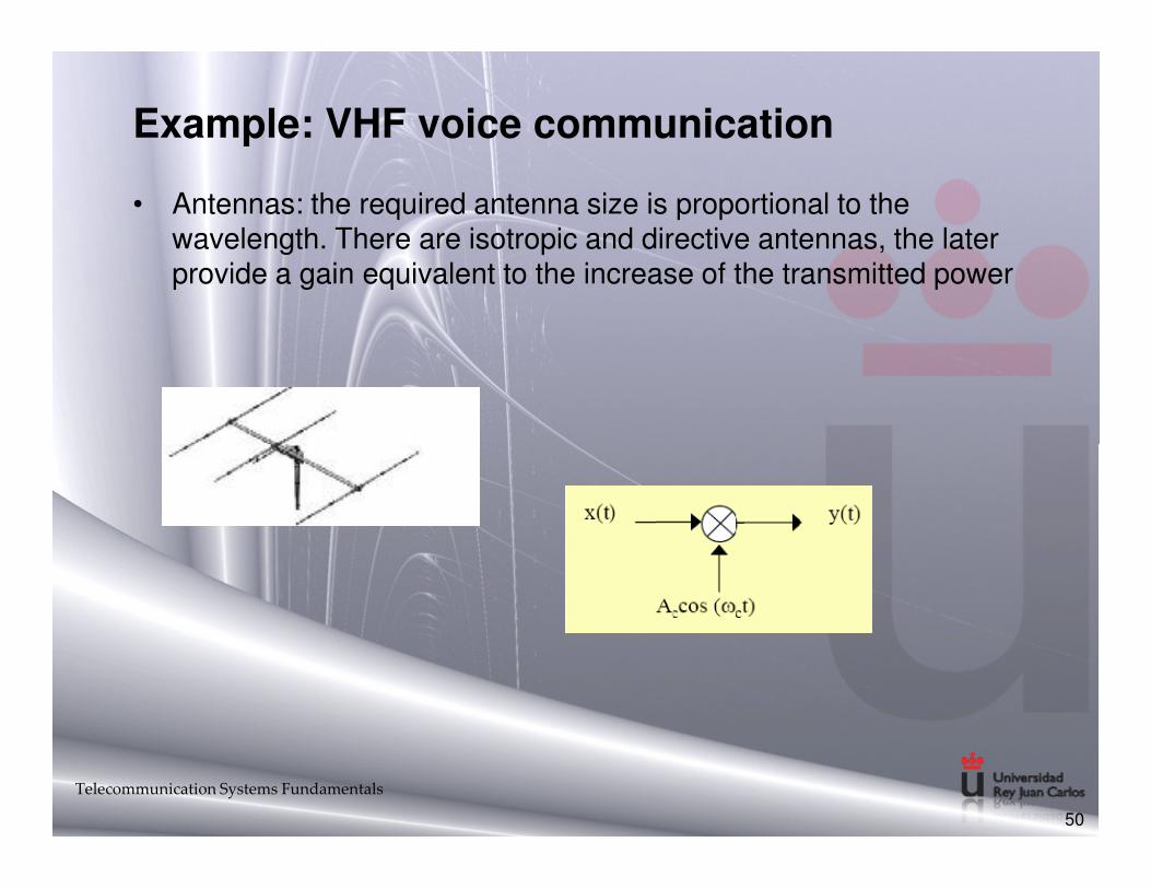
Example: VHF voice communication
• Antennas: the required antenna size is proportional to the wavelength. There are isotropic and directive antennas, the later provide a gain equivalent to the increase of the transmitted power
Telecommunication Systems Fundamentals
50
And from the Antenna to the Air
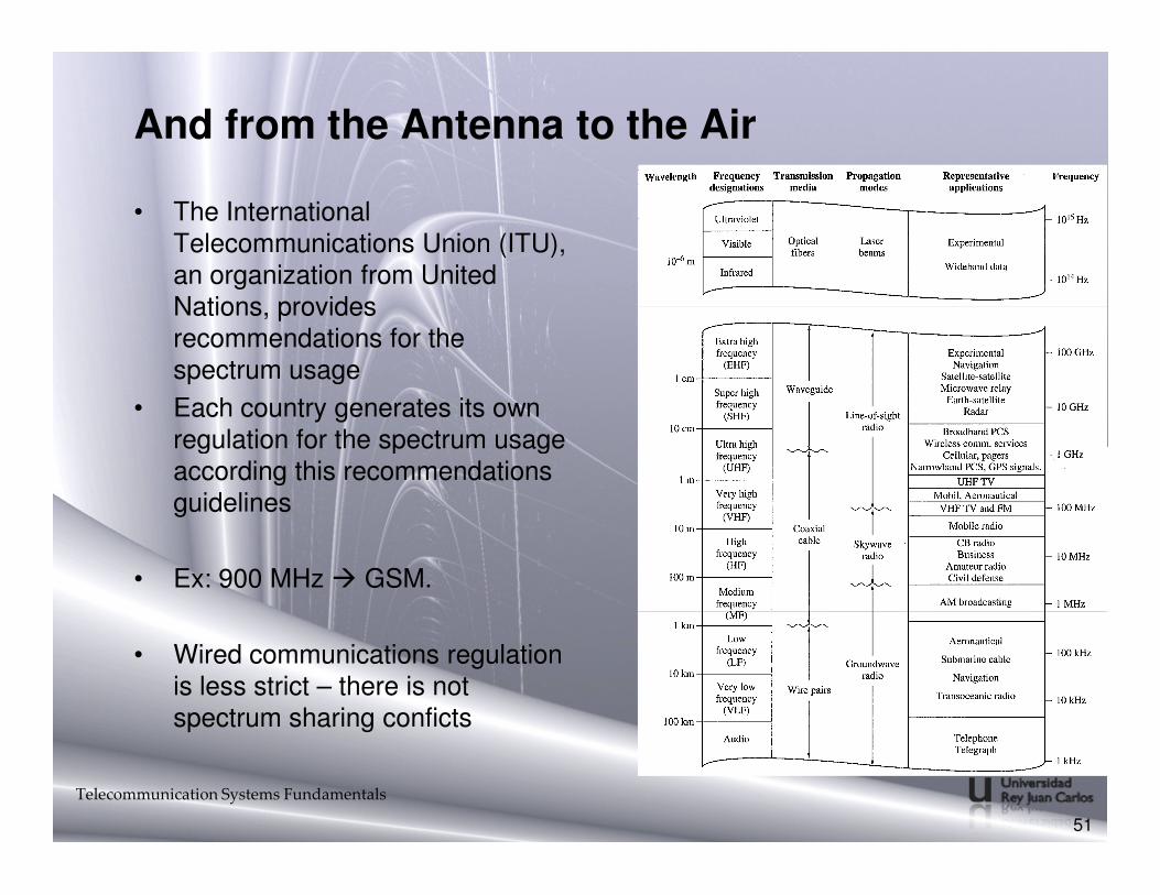
• The International Telecommunications Union (ITU), an organization from United Nations, provides recommendations for the spectrum usage
• Each country generates its own regulation for the spectrum usage regulation for the spectrum usage according this recommendations guidelines
• Ex: 900 MHz ! GSM.
• Wired communications regulation is less strict – there is not spectrum sharing conficts
Telecommunication Systems Fundamentals
51
Modulation Concept
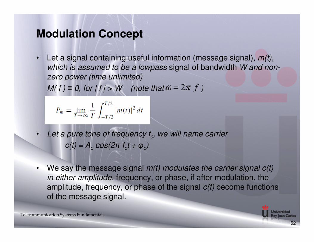
• Let a signal containing useful information (message signal), m(t), which is assumed to be a lowpass signal of bandwidth W and non-zero power (time unlimited)
M( f ) ≡ 0, for | f | > W (note that )fπω 2=
• Let a pure tone of frequency fc, we will name carrier
c(t) = Ac cos(2π fct + φc)
• We say the message signal m(t) modulates the carrier signal c(t) in either amplitude, frequency, or phase, if after modulation, the amplitude, frequency, or phase of the signal c(t) become functions of the message signal.
52
Telecommunication Systems Fundamentals

Modulation Concept
• Modulation converts the message signal m(t) from lowpass to bandpass, in the neighborhood of the center frequency fc with the following objectives:
– The lowpass signal is translated in frequency to the passband of the channel so that the spectrum of the transmitted bandpass signal will match the passband characteristics of the channel;
– To accommodate for simultaneous transmission of signals from – To accommodate for simultaneous transmission of signals from several message sources, by means of frequency-division multiplexing
– To expand the bandwidth of the transmitted signal in order to increase its noise immunity in transmission over a noisy channel
53
Telecommunication Systems Fundamentals
Modulation Types
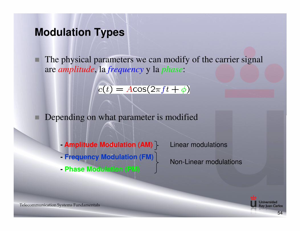
" The physical parameters we can modify of the carrier signal are amplitude, la frequency y la phase:
" Depending on what parameter is modified" Depending on what parameter is modified
Telecommunication Systems Fundamentals
54
- Amplitude Modulation (AM)
- Frequency Modulation (FM)
- Phase Modulation (PM)
Linear modulations
Non-Linear modulations
Analogue vs Digital Modulations
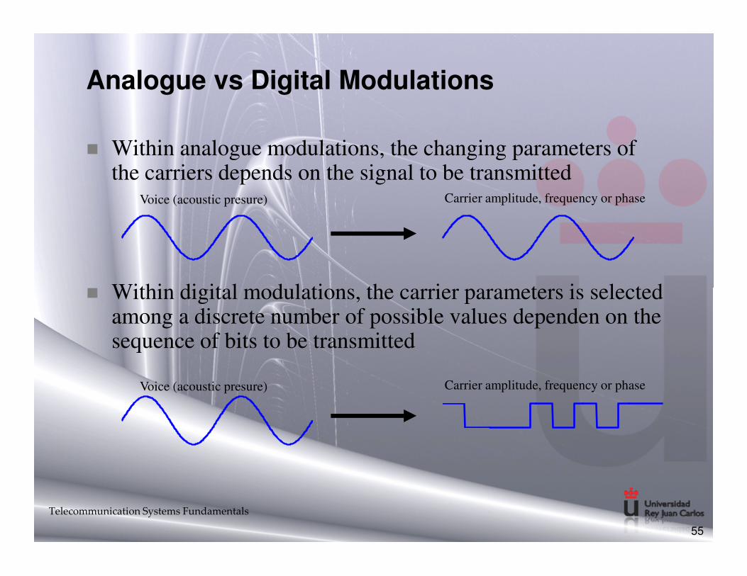
" Within analogue modulations, the changing parameters of the carriers depends on the signal to be transmitted
" Within digital modulations, the carrier parameters is selected
Voice (acoustic presure) Carrier amplitude, frequency or phase
" Within digital modulations, the carrier parameters is selected among a discrete number of possible values dependen on the sequence of bits to be transmitted
Telecommunication Systems Fundamentals
55
Voice (acoustic presure) Carrier amplitude, frequency or phase

Linear Modulations
" Carrier ampluted, c(t), is modified proportionally to the modulating signal, m(t).
Telecommunication Systems Fundamentals
56
Linear Modulations
# Doble Side-Band" DSB-SC (Double-Sideband Supressed Carrier)
" AM (Conventional Amplitude Modulation)
# Single Side-Band" SSB (Single-Sideband)
" VSB (Vestigial Sideband)" VSB (Vestigial Sideband)
Telecommunication Systems Fundamentals
57
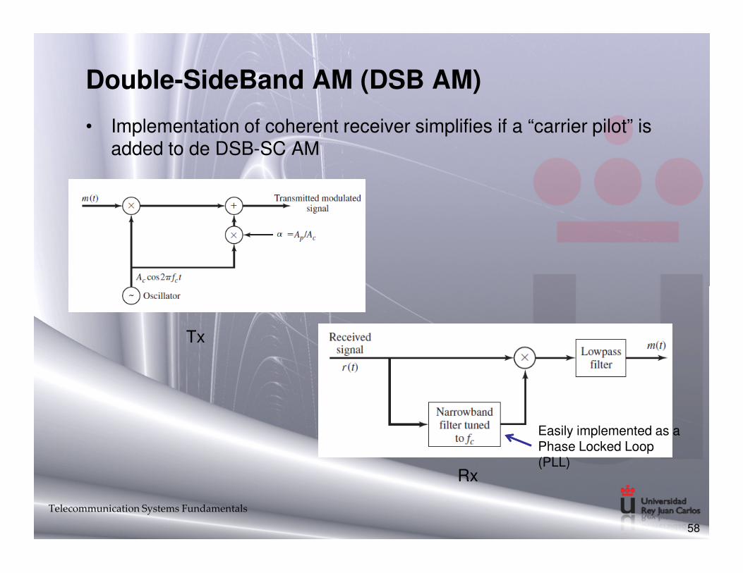
Double-SideBand AM (DSB AM)
• Implementation of coherent receiver simplifies if a “carrier pilot” is added to de DSB-SC AM
58
Tx
Rx
Easily implemented as a Phase Locked Loop (PLL)
Telecommunication Systems Fundamentals
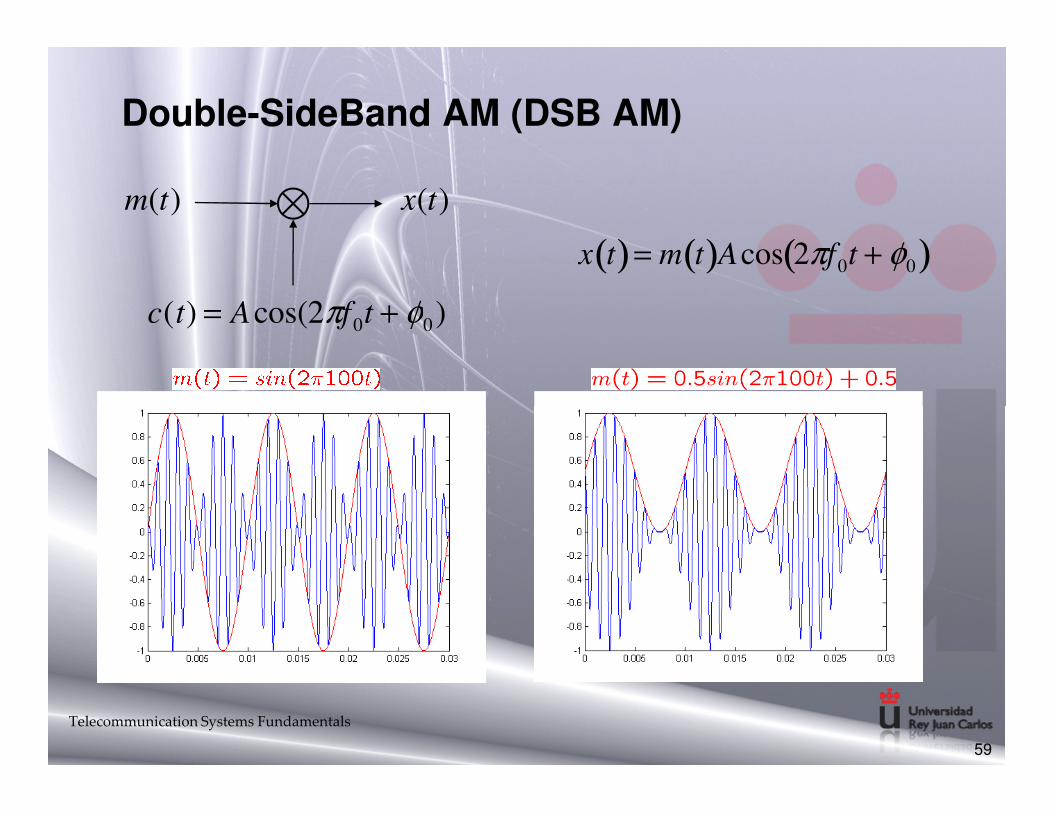
Double-SideBand AM (DSB AM)
)(tm
c(t) = Acos(2πf0t + φ0)
)(tx
x t( )= m t( )Acos 2πf0t + φ0( )
59
Telecommunication Systems Fundamentals
08/10/2013
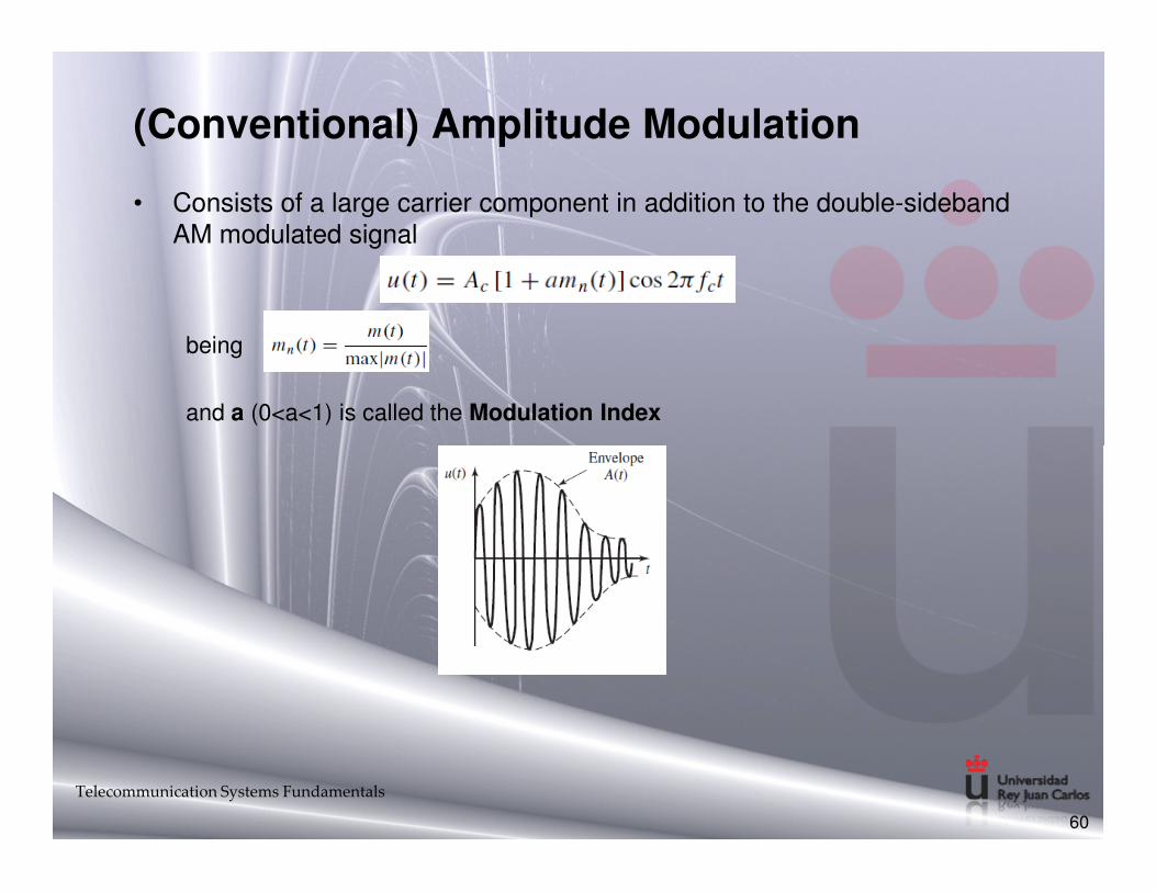
(Conventional) Amplitude Modulation
• Consists of a large carrier component in addition to the double-sidebandAM modulated signal
being
and a (0<a<1) is called the Modulation Index
60
Telecommunication Systems Fundamentals

Single-SideBand Amplitude Modulation(SSB AM)
• where mˆ(t) is the Hilbert transform of m(t) which can be calculated as de convolution of m(t) and a linear filter with impulse response h(t) = 1/πt , so its frequency response is
61
Telecommunication Systems Fundamentals
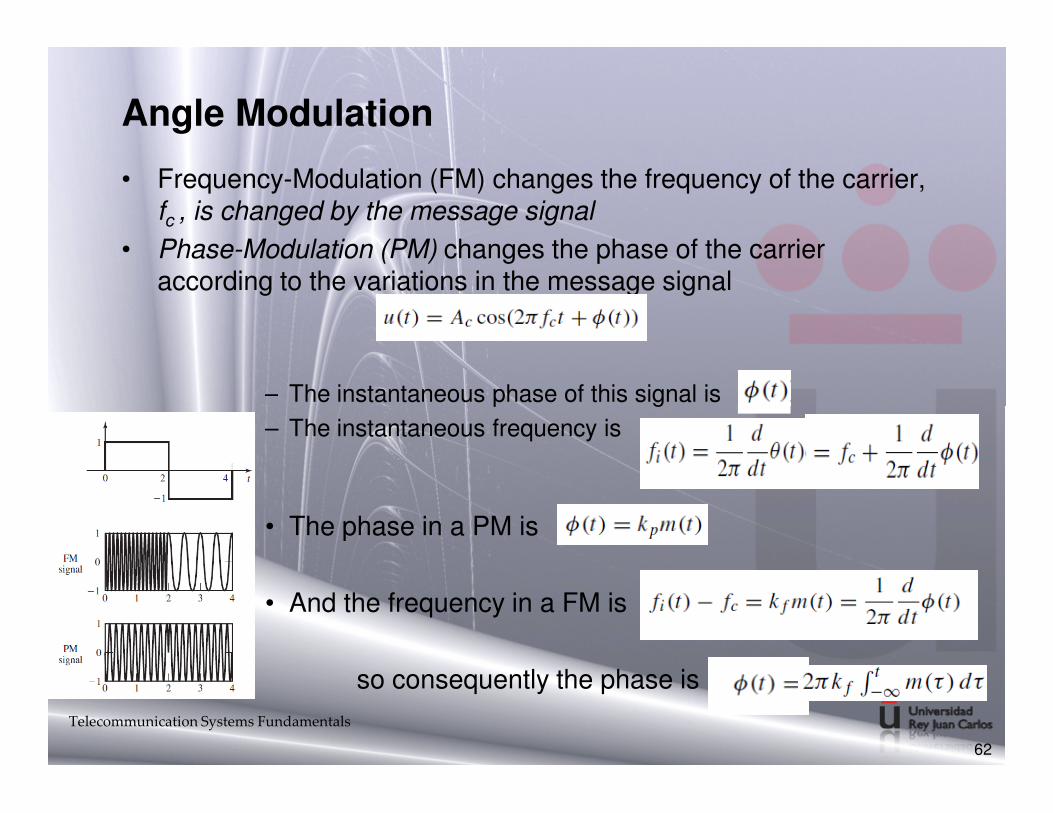
Angle Modulation
• Frequency-Modulation (FM) changes the frequency of the carrier, fc , is changed by the message signal
• Phase-Modulation (PM) changes the phase of the carrier according to the variations in the message signal
– The instantaneous phase of this signal is – The instantaneous phase of this signal is
– The instantaneous frequency is
• The phase in a PM is
• And the frequency in a FM is
so consequently the phase is
62
Telecommunication Systems Fundamentals
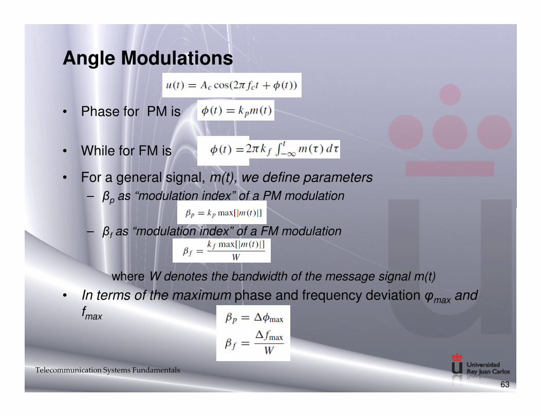
Angle Modulations
• Phase for PM is
• While for FM is
• For a general signal, m(t), we define parameters
– βp as “modulation index” of a PM modulation
– βf as “modulation index” of a FM modulation
where W denotes the bandwidth of the message signal m(t)
• In terms of the maximum phase and frequency deviation φmax and fmax
63
Telecommunication Systems Fundamentals

Summary of Analogue Modulations
Modul.Complexity
BB 1 1 Low
AM 2 Low
W
Bw
BBSNR
SNR
Telecommunication Systems Fundamentals
64
DSB 2 1 High
SSB 1 1 Moderate
VSB 1+ <1 Low
PM Moderate
FM Moderate
Concepts in this Chapter
• General Overview– Logarithmic Units (dB) and Link Budget– Review of fundamental parameters of physical layer: bandwidth, BER, SNR,
Rate…– Other merit figures: Quality of Service– A/D Converter– Circuit Commutation vs. Packet Commutation– Network Topologies
• Functional Block Diagram of Analog Communications link• Functional Block Diagram of a Digital Communications Link
– Block description– Digital Modulations– Multiplexing and Multiple Access
Telecommunication Systems Fundamentals
65
Theory classes: xx sessions (x hours)Problems resolution: 1 session (2 hours)Lab (Matlab): 2 hours

Digital Communications Link
A/D Source Coder Channel Coder
Base Band Modulation
Pass-Band Modulation
RF AmplifierAntenna
Channel
Telecommunication Systems Fundamentals
66
Antenna
RF Demodulator
Pulse Shape Correlator
Channel Decoder
Source Decoder
D/A

Analogue to Digital Converter
• Sampling
• Quantization
• Coding
Telecommunication Systems Fundamentals
67

Digital to Analogue Converter
• At the other end – the Digital to Analogue Converter– Start with a bit stream
– Groups the bits into packets (ex 8 bits provides 256 levels (ex 8 bits provides 256 levels – standard for audio applications)
– With the 8 bits a voltage level is generated holding it for a given time, Tsampling
– Resulting signal is low-pass filtered
Telecommunication Systems Fundamentals
68
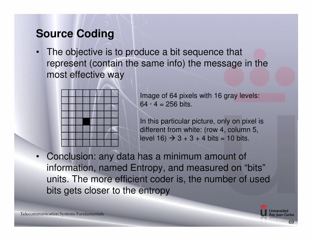
Source Coding
• The objective is to produce a bit sequence that represent (contain the same info) the message in the most effective way
Image of 64 pixels with 16 gray levels: 64 · 4 = 256 bits.
In this particular picture, only on pixel is
• Conclusion: any data has a minimum amount of information, named Entropy, and measured on “bits” units. The more efficient coder is, the number of used bits gets closer to the entropy
Telecommunication Systems Fundamentals
69
In this particular picture, only on pixel is different from white: (row 4, column 5, level 16) ! 3 + 3 + 4 bits = 10 bits.
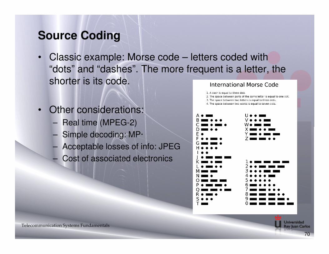
Source Coding
• Classic example: Morse code – letters coded with “dots” and “dashes”. The more frequent is a letter, the shorter is its code.
• Other considerations:– Real time (MPEG-2)– Real time (MPEG-2)
– Simple decoding: MP·
– Acceptable losses of info: JPEG
– Cost of associated electronics
Telecommunication Systems Fundamentals
70
Channel Coding
• Objectives:– To protect the Tx info against channel degradation
– To add redundancy in an efficient way
– To detect and correct errors caused by the channel
• Example: “dumb coder”. Whenever we want to transmit a “1”, the coder generates three “1s” – 111. The receiver gets the three symbols and makes a decision on what was transmitted. If it gets 101, what bit was transmitted?
Telecommunication Systems Fundamentals
71

Channel Coding
• Example: parity check bit
1 0 1 0 1 0 1 0 0
1 0 1 0 1 1 1 0 1
0 0 0 0 0 0 0 0 0
0 1 0 0 0 0 0 0 1
1 0 0 0 1 0 1 0 0
1 0 1 0 1 1 1 0 1
0 0 0 0 0 0 1 0 0
0 1 0 0 0 0 0 0 1
• The number of “1s” is to be even. It detects an odd number of errors. It wastes 11% of the channel capacity
Telecommunication Systems Fundamentals
72
0 1 0 0 0 0 0 0 1
0 0 0 0 0 0 1 0 1
0 0 0 1 1 0 0 0 0
0 1 0 0 0 0 0 0 1
0 0 1 0 0 0 1 0 1
0 0 0 0 0 0 0 0 0

Digital Modulation
• The modulator takes bits and generates signals with the right properties to make it through the channel
• The bit stream is grouped into k bits tuples
• For each of the M = 2k possible bit combination, modulator transmite a different signal sm(t) that last Ts
secondsseconds
• There is a biunivoque correspondece between each combination of M bits (symbol) and the signal transmitted
Telecommunication Systems Fundamentals
73

Digital Modulation
• Dummy example
Telecommunication Systems Fundamentals
74

Detection and Estimation
• General model for digital transmission
– Symbols are transmitted at a rate of R = 1/T (a new symbol is transmitted every T seconds
– Each symbol is transmitted as a different waveform
• Let be a system with M04 different symbols
mi
i = 1,2... M T
si(t) = 0
A
t > Tt < T
• Let be a system with M04 different symbols
75
00 0 T/2
01 T/2 T
10 0 T/2
11 T/2 T
mi si(t)Javier Ramos. Signal Theory and Communications
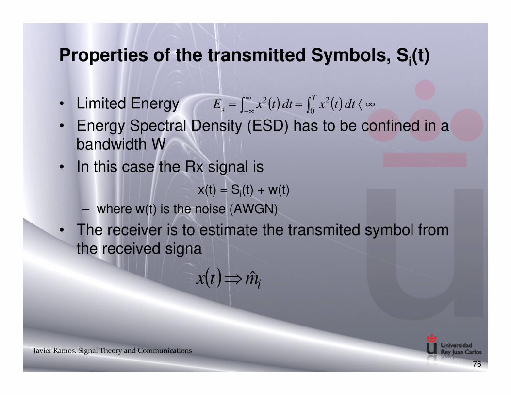
Properties of the transmitted Symbols, Si(t)
• Limited Energy
• Energy Spectral Density (ESD) has to be confined in a bandwidth W
• In this case the Rx signal is
( ) ( ) ∞⟨== ∫ ∫∞
∞−
T
x dttxdttxE0
22
x(t) = Si(t) + w(t)
– where w(t) is the noise (AWGN)
• The receiver is to estimate the transmited symbol from the received signa
76
( ) imtx ˆ⇒
Javier Ramos. Signal Theory and Communications
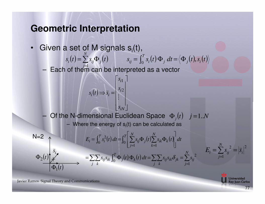
Geometric Interpretation
• Given a set of M signals si(t),
– Each of them can be interpreted as a vector
( ) ( ) ( ) ( ) ( )tstdttsststs ij
T
jiij
N
jjiji ,
01
Φ=Φ=Φ= ∫∑=
( )
=⇒ i
i
ii
s
s
stsM
2
1
– Of the N-dimensional Euclidean Space– Where the energy of si(t) can be calculated as
77
iNs
( )t2Φ
( )t1Φ
is
N=2 ( ) ( ) ( )
( ) ( ) ∑∑∑∑∑ ∫
∫ ∑∑∫
=
==
==ΦΦ=
ΦΦ==
N
jij
j kjkikij
j k
T
kjikij
TN
kkik
N
jjij
T
ii
sssdtttss
dttstsdttsE
1
2
0
011
0
2
δ
2
1
2
i
N
jiji ssE ==∑
=
Javier Ramos. Signal Theory and Communications
( ) Njtj ..1=Φ

Optimum Receiver using Correlators
• Reveived signal can be modelated as
• Correlation during interval [0,T] between x(t) y Φ (t) is
( )tx
( )tjΦ
∫T
0 T
yj ( ) ( )∫ Φ=T
jj dtttxy0
( ) ( ) ( )
( ) ≡
=
+=
tw
Mi
twtstx i
,...1
AWGN of PSD N0/2
• Correlation during interval [0,T] between x(t) y Φj(t) is computed, resulting
78
( ) ( ) ( ) ( ) ( ) ( )∫ Φ+∫ Φ=Φ= ∫ Tj
Tji
T
jj dtttwdtttsdtttxy 000
=sij Gaussian Random Variable
- mean- variance
Javier Ramos. Signal Theory and Communications

Optimum Receiver with a Bank of Correlators
[ ] ( )( )[ ]ikkijjkj sysyEyyCov −−=, ( ) ( ) ( ) ( )[ ]=ΦΦ= ∫∫T
j
T
j duuuwdtttwE00
,
( )tx( )t1Φ
y1= si1+ w1
( )t2Φ∫
T
0
∫T
0
y2= si2+ w2
•••
•••
•••
79
( ) 0, =kj yyCov <==> yj,yk are uncorrelated
Two uncorrelated and Gaussiand RV are Independet
00
( ) ( )22
0
0
0 Ndttt
Njk
T
kj δ=ΦΦ= ∫[ ]
[ ]
=
=
ikkj
ijj
NyyCov
syE
δ2
, 0
( ) ( )[ ] ( ) ( ) =ΦΦ= ∫ ∫ dudtutuwtwE kj
T T
0 0( ) ( ) ( ) =ΦΦ−= ∫ ∫
T T
kj dudtututN
0 0
0
2δ
Javier Ramos. Signal Theory and Communications

Optimum Detection
• Decission Zone for symbol i– Locus of points which distance to point si is smaller than to any
other point of the constellation
Φ2
z =
+−=−= ∑∑∑NNN
ssyyminsyminm222
2ˆ
80
s1s2 Φ1
z1
z2
=+−=−= ∑∑∑
=== jij
jijj
jj
mi
mssyyminsyminm
ii 111
2ˆ
−=
+−= ∑∑
==
N
jiijj
m
N
jiijj
mEsymaxEsymin
ini 11 2
12
Javier Ramos. Signal Theory and Communications

Error Probability and Optimum Detection
• Defining a new orthonormal basis which axis passes through both points d i k (distancia entre símbolos)
si sk Φi’(t)di k /2
( )
=′′2
, Gausiano / 0Nsmyf iiy
( ) ( )( )
===−
∞
∫'
111/ 0
2
derfcemmPAP ikN
y
duexerfc u
x
22)( −
∞
∫=π
• and applying the Union Upper Bound, the error probability of mi
symbol becomes
• Thus, the system total probability of error
81
( ) ( )
=== ∫0
2/0 2
1
2
11/ 0
N
derfce
NmmPAP ikN
dikikik π
( ) ∑≠=
=
M
ikik
iki
N
derfcmPe
02
1
2
1
∑ ∑=
≠=
=
M
i
M
ikik
ik
N
derfc
MPe
1 02
1
2
11
Javier Ramos. Signal Theory and Communications

Error Probability and Optimum Detection
• Defining again the minimum distance as
– and using the inequality
ik
kiki
min dmind
≠
=,
( )
−≤
∑≠= 01 0 2
12 N
derfcM
N
derfc min
M
kik
ik
• The Union Upper Bound for de Symbol Error Probability results as
82
≠
00ki
( )
−≤
022
1
N
derfc
MPe min
Javier Ramos. Signal Theory and Communications
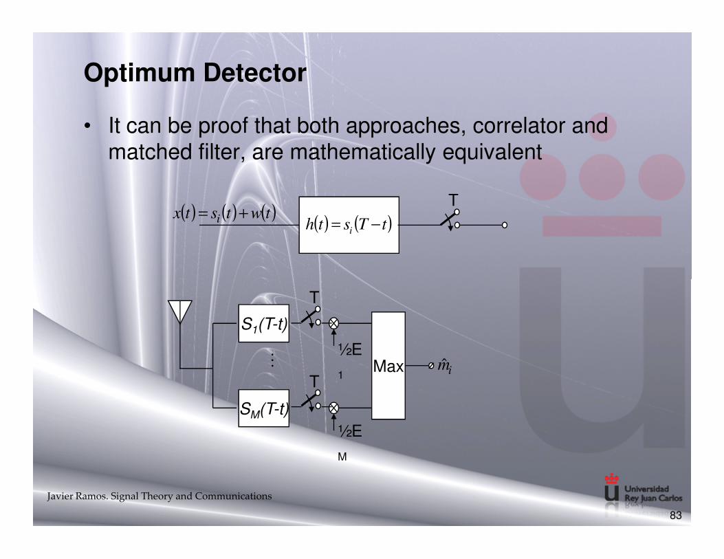
Optimum Detector
• It can be proof that both approaches, correlator and matched filter, are mathematically equivalent
( ) ( ) ( )twtstx i +=( ) ( )tTsth i −=
T
83
S1(T-t)
Mim̂
½E
1
½E
M
Max
SM(T-t)
T
T
Javier Ramos. Signal Theory and Communications

Base-Band Transmission
• Some systems require transmitted signal to have its spectrum around DC frequency – Base-Band Transmission
mi
i=1,...M si(t) = 0 ( )[ ]2
tSTFH isi=
0 f
isH
• General denomination for the most common modulations in base-band: PAM (Pulse Amplitude Modulation)
84
0 f
mi si(t) = ai•s(t) Example a
“1”
“0”
Javier Ramos. Signal Theory and Communications

PAM
• Signal types depending on the pulse shape, s(t)– NRZ (Non Return to Zero)
– Manchester or Bi-Phase
s(t) ≠ 0 0 ≤ t ≤ T
example: 0 T
s(t) ) = - s(t+T/2) 0 ≤ t ≤ T
– RZ (Return to Zero
85
s(t) ) = - s(t+T/2) 0 ≤ t ≤ T
example: 0 T
s(t) = 0 ti ≤ t ≤ T
example: 0 T/2 T
Javier Ramos. Signal Theory and Communications

PAM
• Signal types depending on the aplitudes, ai
– Unipolar ai ≥ 0 ∀ i Examples: Binary Unipolar NRZ
ai =1 si m1
0 si m0 0 1 0
Binary Unipolar NRZ
– Polar ai = - ai + M/2
86
Binary Unipolar NRZ
ai =1 si m1
5 si m0
Binary polar NRZ
1 0 1 1
Quaternary Polar NRZ
00 01 10 11
Javier Ramos. Signal Theory and Communications
PAM
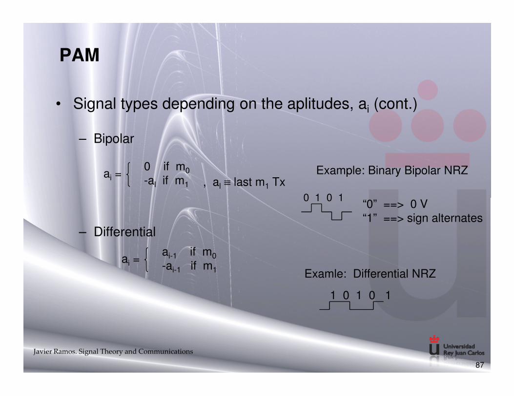
• Signal types depending on the aplitudes, ai (cont.)
– Bipolar
ai =0 if m0
-al if m1
Example: Binary Bipolar NRZ, al ≡ last m1 Tx
0 1 0 1“0” ==> 0 V
– Differential
87
Javier Ramos. Signal Theory and Communications
0 1 0 1“0” ==> 0 V“1” ==> sign alternates
ai =ai-1 if m0
-ai-1 if m1 Examle: Differential NRZ
1 0 1 0 1

M-PAM
• Númer of possible symbols, M, may be different to 2– Then Symbol and Bit take different meaning
– If symbol duration is T, then the symbol rate is R = 1/T and
MRR b
log
1⋅=
88
MTT b 2log≡
M2log
Javier Ramos. Signal Theory and Communications
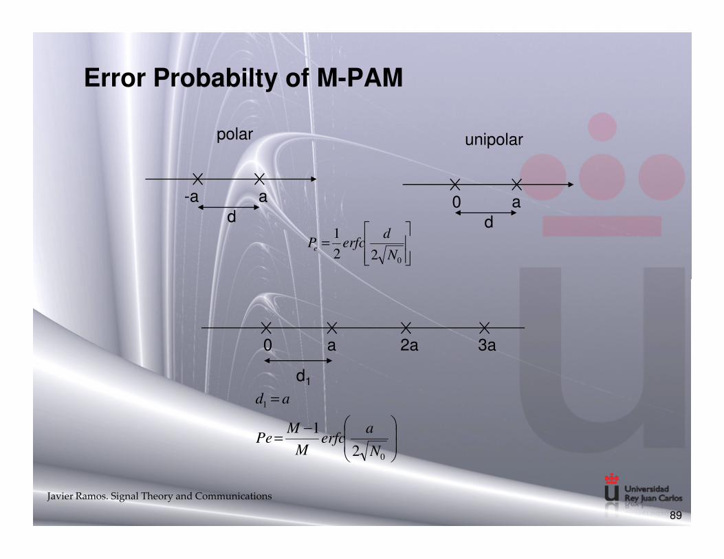
Error Probabilty of M-PAM
-a ad
polar
0 ad
unipolar
=
022
1
N
derfcPe
89
Javier Ramos. Signal Theory and Communications
−=
=
0
1
2
1
N
aerfc
M
MPe
ad
d1
0 a 2a 3a
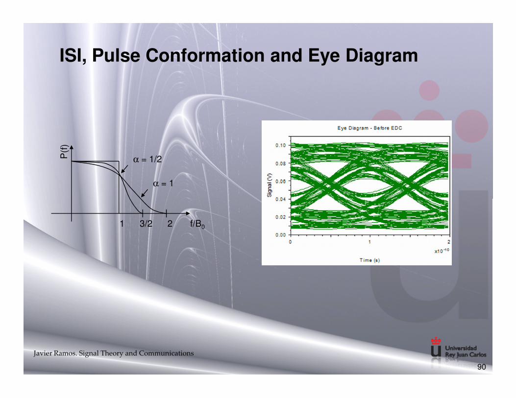
ISI, Pulse Conformation and Eye Diagram
α = 1/2
α = 1
P(f
)
90
Javier Ramos. Signal Theory and Communications
1 3/2 2 f/B0
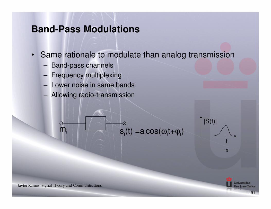
Band-Pass Modulations
• Same rationale to modulate than analog transmission– Band-pass channels
– Frequency multiplexing
– Lower noise in same bands
– Allowing radio-transmission
91
mi si(t) =aicos(ωit+ϕi)|S(f)|
f
0
Javier Ramos. Signal Theory and Communications
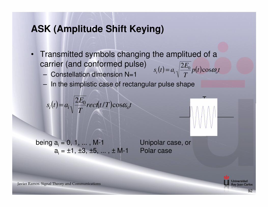
ASK (Amplitude Shift Keying)
• Transmitted symbols changing the amplitued of a carrier (and conformed pulse)– Constellation dimension N=1
– In the simplistic case of rectangular pulse shape
( ) ( ) ttpT
Eats oii ωcos
2 0=
( ) ( ) tTtrectE
ats ωcos/2 0=
T
92
( ) ( ) tTtrectT
Eats oii ωcos/
2 0=
being ai = 0, 1, ... , M-1 Unipolar case, orai = ±1, ±3, ±5, ... , ± M-1 Polar case
Javier Ramos. Signal Theory and Communications
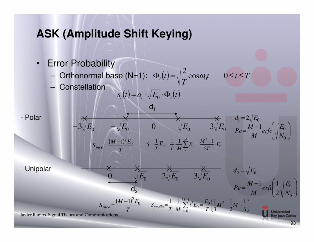
ASK (Amplitude Shift Keying)
• Error Probability– Orthonormal base (N=1):
– Constellation
( ) TttT
ti ≤≤=Φ 0cos2
0ω
( ) ( )tEats iii Φ⋅⋅= 0
- Polar
−−
d1
= 01 2 Ed
93
- Polar
- Unipolar
0000 303 EEEE −−
000 320 EEE
d2
Javier Ramos. Signal Theory and Communications
−=
=
0
0
01
1
2
N
Eerfc
M
MPe
Ed
−=
=
0
0
02
2
11
N
Eerfc
M
MPe
Ed
( )T
EMSpico
02
1−= 0
2
1 2
1111E
T
ME
MTE
TS
M
i
sisi ⋅−
=⋅== ∑=
( )T
EMSpico
021−
=
+−=⋅= ∑−
= 6
1
2
1
3
111 201
00
2 MMT
EEi
MTS
M
imedia
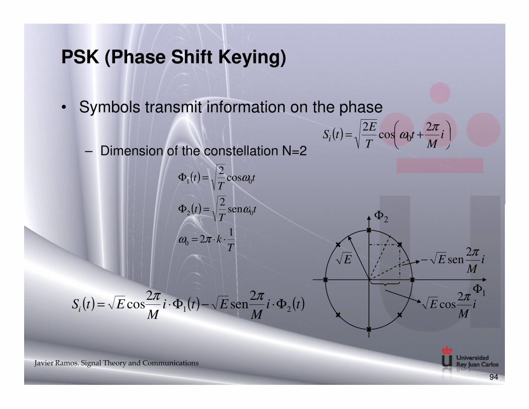
PSK (Phase Shift Keying)
• Symbols transmit information on the phase
– Dimension of the constellation N=2
( )
+= iM
tT
EtSi
πω
2cos
20
( )
( ) tt
tT
t
sen2
cos2
01
=Φ
=Φ
ω
ω
94
( )
Tk
tT
t
12
sen2
0
02
⋅⋅=
=Φ
πω
ω
( ) ( ) ( )tiM
EtiM
EtSi 21
2sen
2cos Φ⋅−Φ⋅=
ππ
Javier Ramos. Signal Theory and Communications
2Φ
1Φ
E
iM
Eπ2
cos
iM
Eπ2
sen−

PSK (Phase Shift Keying)
• Error Probability
– Realizing on the rotational symetry
( )( )
( )
dydxeNM
mPeM
Pe N
yEx
z
M
ii
i
0
22
01
111+−
−
=∫∫∑ ==
π
iz
for M ≥ 4:
≈
Msin
N
EerfcPe
π
0
– Union Upper bound
95
MN0
MEdmin
π2cos12 −⋅=
−⋅
−=
−⋅
−=
MN
Eerfc
M
MN
Eerfc
MPe
ππ 2cos1
22
12cos1
2
2
1
2
1
00
Javier Ramos. Signal Theory and Communications

PSK (Phase Shift Keying)
BPSK (M = 2)
1Φ
E
=
02
1
N
EerfcPe
96
( )t2Φ
( )t1Φ
QPSK (M = 4)
2Φ
1Φ
ó
=
02N
EerfcPe
Javier Ramos. Signal Theory and Communications
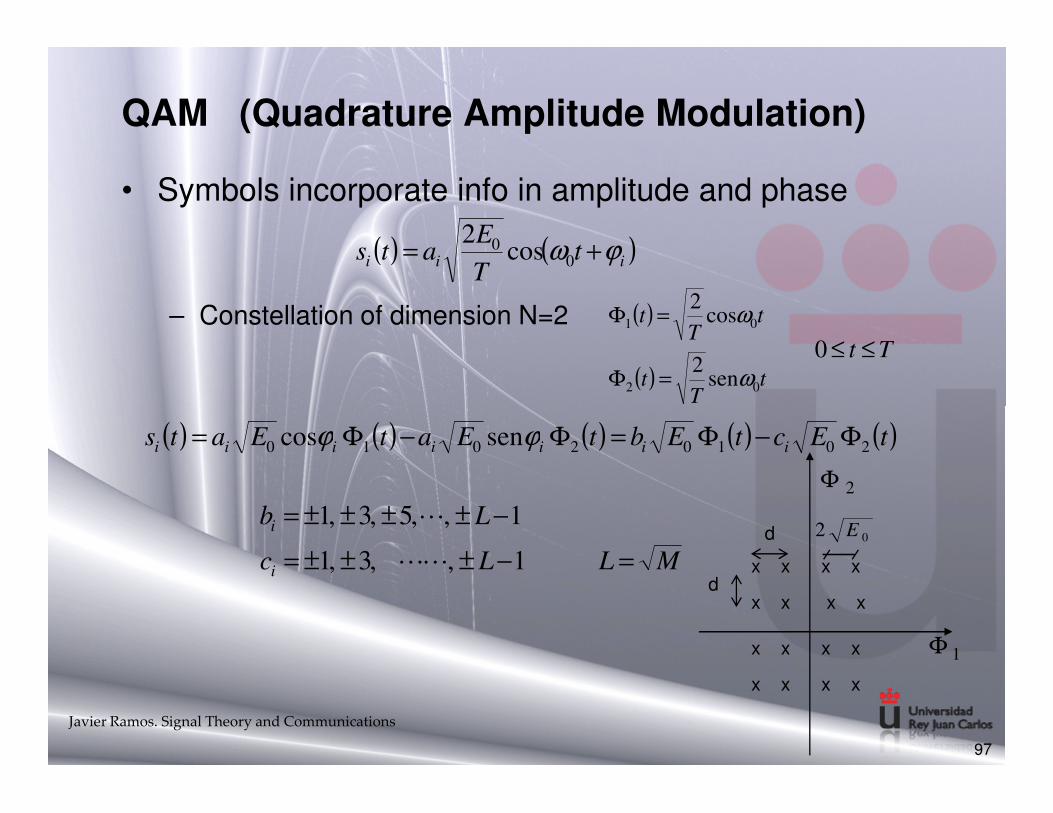
QAM (Quadrature Amplitude Modulation)
• Symbols incorporate info in amplitude and phase
– Constellation of dimension N=2
( ) ( )iii tT
Eats ϕω += 0
0 cos2
( )
( ) tT
t
tT
t
02
01
sen2
cos2
ω
ω
=Φ
=Φ
Tt ≤≤0
97
T
( ) ( ) ( ) ( ) ( )tEctEbtEatEats iiiiiii 20102010 sencos Φ−Φ=Φ−Φ= ϕϕ
MLLc
Lb
i
i
=−±±±=
−±±±±=
1,,3,1
1,,5,3,1
LL
L
Javier Ramos. Signal Theory and Communications
x x x x
x x x x
x x x x
x x x x
2Φ
1Φ
d
d
02 E
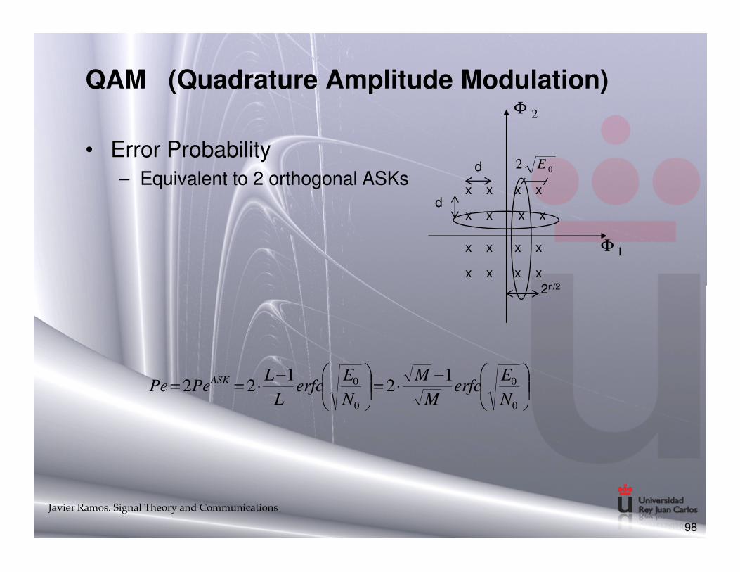
QAM (Quadrature Amplitude Modulation)
• Error Probability– Equivalent to 2 orthogonal ASKs
x x x x
x x x x
x x x x
x x x x
2Φ
1Φ
d
d
02 E
2n/2
98
2n/2
−⋅=
−⋅==
0
0
0
0 12
122
N
Eerfc
M
M
N
Eerfc
L
LPePe ASK
Javier Ramos. Signal Theory and Communications
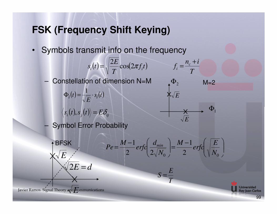
FSK (Frequency Shift Keying)
• Symbols transmit info on the frequency
– Constellation of dimension N=M
( ) ( )tfT
Ets ii π2cos
2=
E
2Φ
Φ
T
inf c
i
+=
( ) ( )tsE
t ii ⋅=Φ1
M=2
– Symbol Error Probability
99
E
1Φ( ) ( ) ijji Etsts δ=,
Javier Ramos. Signal Theory and Communications
E
E
dE =2
BFSK
−=
−=
00 2
1
22
1
N
Eerfc
M
N
derfc
MPe min
T
ES =

Spectral Efficiency and Bandwidth
B
Rb=ρ
• ASK,PSK,QAM
MTTB
b 2log
22==
2
log
log/2
/1 2
2
M
MT
T
b
b ==ρ
• MSKMTb 2log2/1
==ρMMB11
==
100
M
M
MT
Tb 2log2
2/1
/1=
⋅=ρM
MTM
TB
b 2log2
1
2
1==
• FSK
M
M2log=ρM
MTM
TB
b
⋅==2log2
1
2
1
(asuming rectangular pulses and Bandwidth to the first null)
Javier Ramos. Signal Theory and Communications
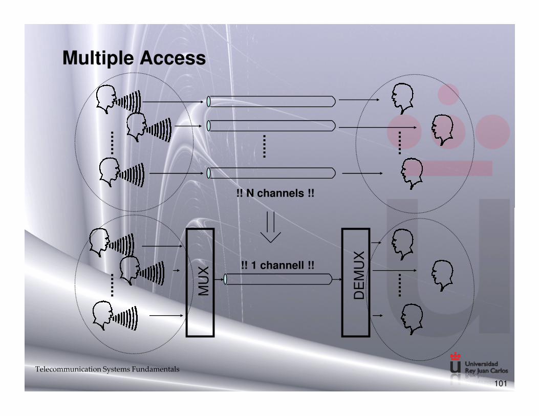
Multiple Access
!! N channels !!
Telecommunication Systems Fundamentals
101
MU
X
DE
MU
X
!! 1 channell !!
Multiple Access
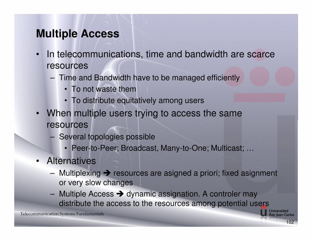
• In telecommunications, time and bandwidth are scarce resources– Time and Bandwidth have to be managed efficiently
• To not waste them
• To distribute equitatively among users
• When multiple users trying to access the same resourcesresources– Several topologies possible
• Peer-to-Peer; Broadcast, Many-to-One; Multicast; …
• Alternatives– Multiplexing $ resources are asigned a priori; fixed asignment
or very slow changes
– Multiple Access $ dynamic assignation. A controler may distribute the access to the resources among potential users
Telecommunication Systems Fundamentals
102
Duplexing
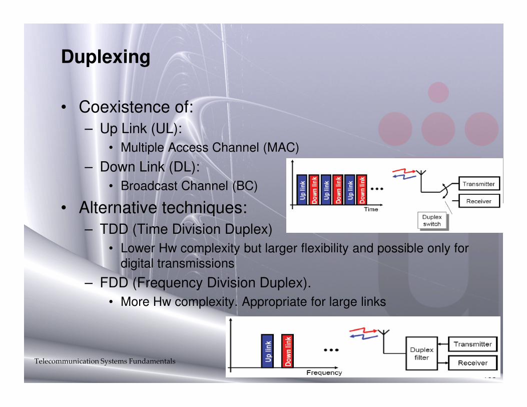
• Coexistence of:– Up Link (UL):
• Multiple Access Channel (MAC)
– Down Link (DL):
• Broadcast Channel (BC)
• Alternative techniques:• Alternative techniques:– TDD (Time Division Duplex)
• Lower Hw complexity but larger flexibility and possible only for digital transmissions
– FDD (Frequency Division Duplex).
• More Hw complexity. Appropriate for large links
Telecommunication Systems Fundamentals
103
Multiple Access
• Contentionless Techniques (supervised) :– Resources Pre-assigned to users
– Pre-established rules
– Deterministic access
– Adequate for regular streams
– Capable to guaranty the QoS, but risk of outage– Capable to guaranty the QoS, but risk of outage
• Contention Techniques (under demand):– Users decide when to take resources from the channel
– Stochastic access
– Adequate for irregular streams
Telecommunication Systems Fundamentals
104

Contentionless Techniques (supervised)
• Usefull when there is infrastructure and the users transmit regularly
• It requires larger maintenance but performance is guarantied
• Clear rules about when a user should transmit• Clear rules about when a user should transmit
• Different users can be discrimitaed by– Frequency: FDMA
– Time: TDMA
– Code: CDMA
– Space: SDMA
Telecommunication Systems Fundamentals
105
Frequency Division Multiple Access. FDMA.
Signal at the Channel
t
User 1 Tx Signal
User 2 Tx Signal
106
t
Tx Signal
User N Tx Signal
!Simultaneous Transmission of all Users!t
t
Telecommunication Systems Fundamentals
ff1
Frequency Division Multiple Access. FDMA.
107
ff2
ff1 f2 fN
ffNTelecommunication Systems Fundamentals

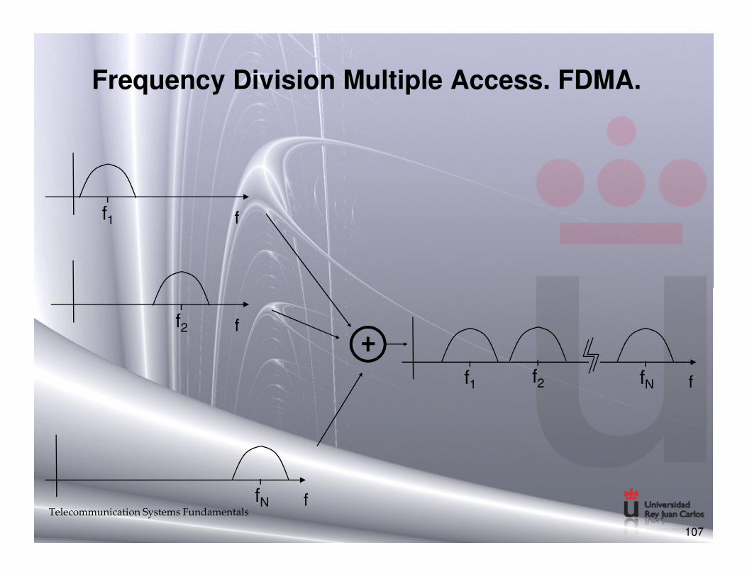
Frequency Division Multiple Access. FDMA.
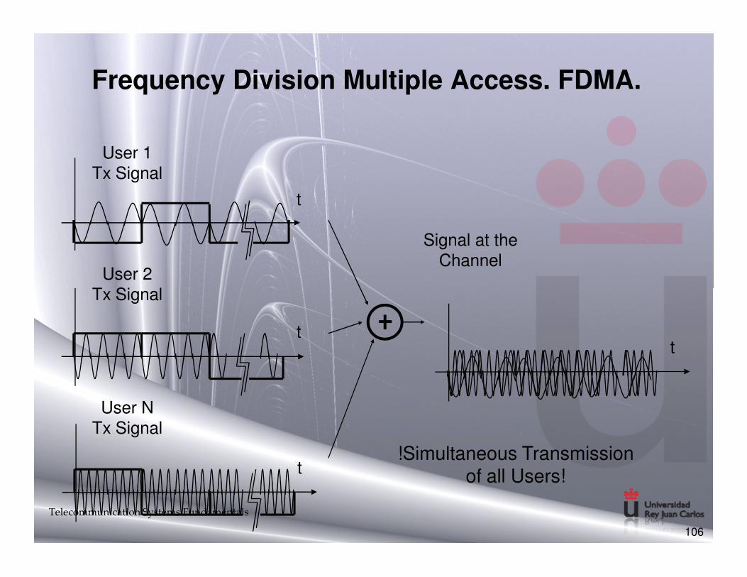
• Available Bandwidth is divided into sub-bands
– Each user is assigned to a sub-band $ orthogonal access
• Characteristics
– Simple time synchronization
– Strict frequency alignment required
– Sensible to frequency alterations: Doppler shift, intermodulations, clock drift, etc.
• Used on• Used on
– Analogue systems
– Broadband access where the sub-band assigned are large
– Large radio coverage where time division show low efficiency
– Combination with other Multiple Access techniques
• Alterations:
– OFDMA:
• Each OFDM user is assigned with a different sub-carrier set
– SC-FDMA:
• Similar to OFDM but pre-coding symbols using a DFT
• Gets some advantages and better performance
Telecommunication Systems Fundamentals
108
Time Division Multiple Access. TDMA.
• Each user is assigned different time interval – time slot– Orthogonal Access
• Characteristics– Complex Time synchronization
– Simple frequency synchronization
– Each user occupies all the available bandwidth, so it can cope easily with frequency selective fading – interleavingeasily with frequency selective fading – interleaving
– Users can use non-transmitting slots to measure the channel or perform other signaling tasks
• Typically combined with FDMA– Example: GSM.
• Typical Base Station: 3 freqyency channels (duplex) (FDMA), each channel shared by 8 users using TDMA $ Each BS can serve 24 simultaneous users
Telecommunication Systems Fundamentals
109

Time Division Multiple Access. TDMA.
Signal at the Channel
t
Bits from User 1
0 1 0
Bits from User 2
110
tt
t
1 1 0
1 0 0
User 1 bitstream: 0 1
User 2
Bits from User N
User 2 bitstream: 1 0
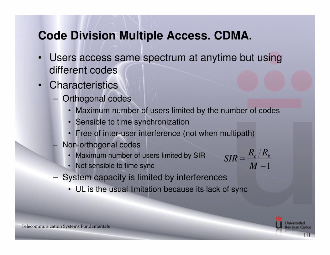
Code Division Multiple Access. CDMA.
• Users access same spectrum at anytime but using different codes
• Characteristics– Orthogonal codes
• Maximum number of users limited by the number of codes
• Sensible to time synchronization
• Free of inter-user interference (not when multipath)
– Non-orthogonal codes
• Maximum number of users limited by SIR
• Not sensible to time sync
– System capacity is limited by interferences
• UL is the usual limitation because its lack of sync
Telecommunication Systems Fundamentals
111
1−=
M
RRSIR bc

Code Division Multiple Access. CDMA.
t t
x Code 1Signal Tx by user 1
Bits from User 1
Bits from User 2 Signal Tx by user 2
112
t
t
t
t
x Code 2
x Code 3
User 2
Bits from User N
Signal Tx by user 2
Signal Tx by user N

Code Division Multiple Access. CDMA.
t
Signal at the Channel
Signal Tx by user 1
113
t
t
t
Signal Tx by user 2
Signal Tx by user N
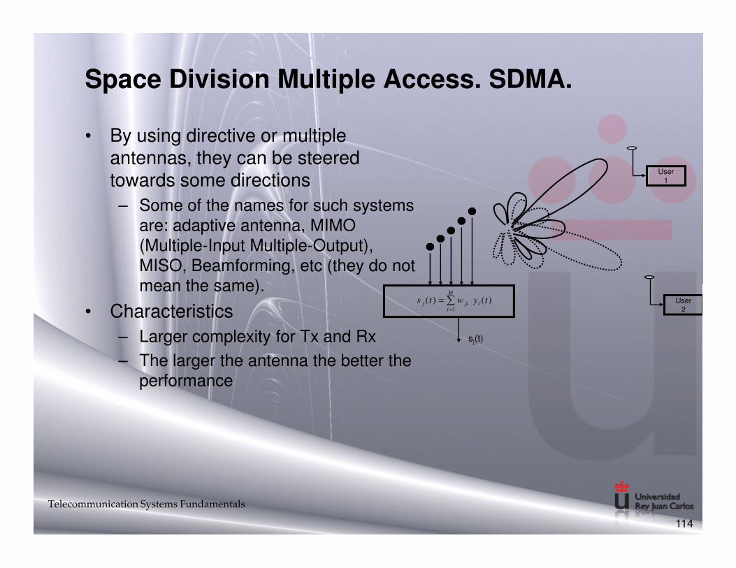
Space Division Multiple Access. SDMA.
• By using directive or multiple antennas, they can be steered towards some directions
– Some of the names for such systems are: adaptive antenna, MIMO (Multiple-Input Multiple-Output), MISO, Beamforming, etc (they do not mean the same).
User1
mean the same).
• Characteristics
– Larger complexity for Tx and Rx
– The larger the antenna the better the performance
Telecommunication Systems Fundamentals
114
∑=
=M
iijij tywts
1
)()(
sj(t)
User2

Contention Multiple Access (Unsupervised)
• Under demand techniques– No pre-assignment of resources $ users decide when
transmit
– Users may collide - collision
• Effective when users streams are irregular (burst traffic)traffic)– Probabilistic access
– Not possible to guaranty instantaneous QoS
• Widely used because its simplicity and efficiency– Local Area Networks: ex. Ethernet or WiFi
• Most common techniques– Aloha / Slotted Aloha
– Carrier Sense Multiple Access (CSMA)
Telecommunication Systems Fundamentals
115

Contention Protocols
• ALOHA– Developed in the 1970s for a packet radio network by Hawaii
University.
– Whenever a station has a data, it transmits
– Sender finds out whether transmission was successful or experienced a collision by listening to the broadcast from the destination stationdestination station
– Sender retransmits after some random time if there is a collision.
• Slotted ALOHA– Improvement: Time is slotted and a packet can only be
transmitted at the beginning of one slot
– It reduces the collision probability
116
Telecommunication Systems Fundamentals
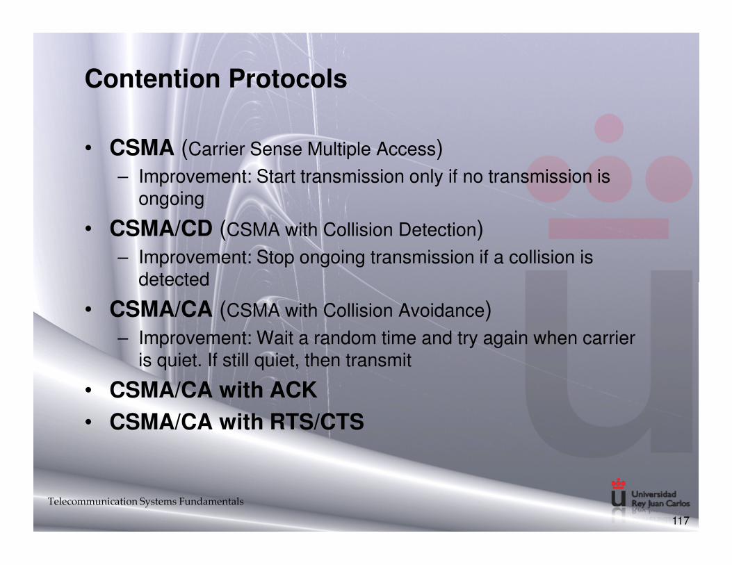
Contention Protocols
• CSMA (Carrier Sense Multiple Access)– Improvement: Start transmission only if no transmission is
ongoing
• CSMA/CD (CSMA with Collision Detection)– Improvement: Stop ongoing transmission if a collision is
detecteddetected
• CSMA/CA (CSMA with Collision Avoidance)– Improvement: Wait a random time and try again when carrier
is quiet. If still quiet, then transmit
• CSMA/CA with ACK
• CSMA/CA with RTS/CTS
117
Telecommunication Systems Fundamentals
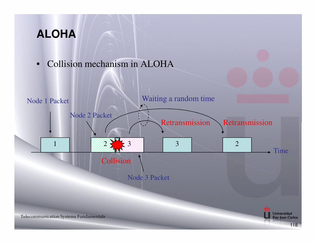
ALOHA
• Collision mechanism in ALOHA
Retransmission Retransmission
Node 1 Packet Waiting a random time
Node 2 Packet
Telecommunication Systems Fundamentals
118
1 2 3 3 2Time
Collision
Retransmission Retransmission
Node 3 Packet
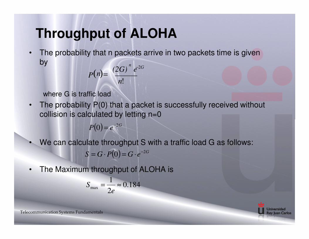
Throughput of ALOHA
• The probability that n packets arrive in two packets time is given by
where G is traffic load
• The probability P(0) that a packet is successfully received without collision is calculated by letting n=0
n
( )!n
(2G)nP
e 2G−
=
• We can calculate throughput S with a traffic load G as follows:
• The Maximum throughput of ALOHA is
( ) GeP 20 −=
( ) GeGPGS 20 −⋅=⋅=
184.02
1max ≈=
eS
Telecommunication Systems Fundamentals

Slotted ALOHA
• Collision mechanism in slotted ALOHA
Retransmission Retransmission
Node 1 Packet
Nodes 2 & 3 Packets
120
1 2&3 2Time
Collision
Retransmission Retransmission
3
Slot
Telecommunication Systems Fundamentals

Throughput of Slotted ALOHA
• The probability of no collision is given by
• The throughput S is
( ) GeP −=0
( ) GeGPGS −⋅=⋅= 0
• The Maximum throughput of slotted ALOHA is
121
( ) GeGPGS −⋅=⋅= 0
368.01
max ≈=e
S
Telecommunication Systems Fundamentals
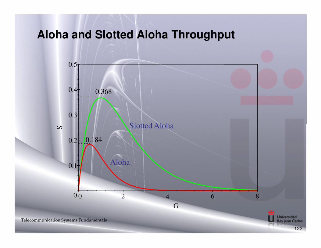
Aloha and Slotted Aloha Throughput
Slotted Aloha
0.368
0.5
0.4
0.3
122
Telecommunication Systems Fundamentals
Slotted Aloha
Aloha
0.184
G
S
8620
0.2
0.1
0 4

CSMA (Carrier Sense Multiple Access)
• Max throughput achievable by slotted ALOHA is 0.368.
• CSMA gives improved throughput compared to Aloha protocols.
• Listens to the channel before transmitting a packet (avoid avoidable collisions).
123
Telecommunication Systems Fundamentals

CSMA
• Collision Mechanism
Node 5 senseNode 1 Packet
Node 2 Packet
124
1 2 3Time
Collision
4
Node 4 sense
Delay
5
DelayNode 2 Packet
Node 3 Packet
Telecommunication Systems Fundamentals
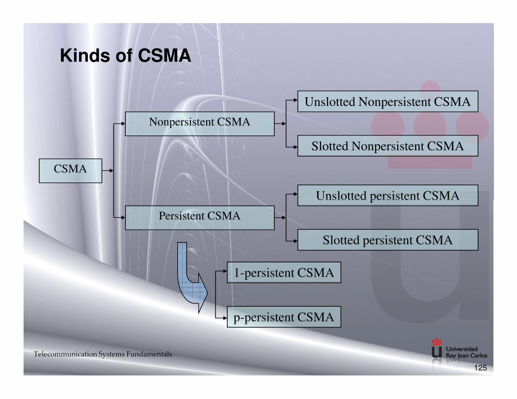
Kinds of CSMA
CSMA
Nonpersistent CSMA
Unslotted Nonpersistent CSMA
Unslotted persistent CSMA
Slotted Nonpersistent CSMA
125
Persistent CSMA
Unslotted persistent CSMA
Slotted persistent CSMA
1-persistent CSMA
p-persistent CSMA
Telecommunication Systems Fundamentals
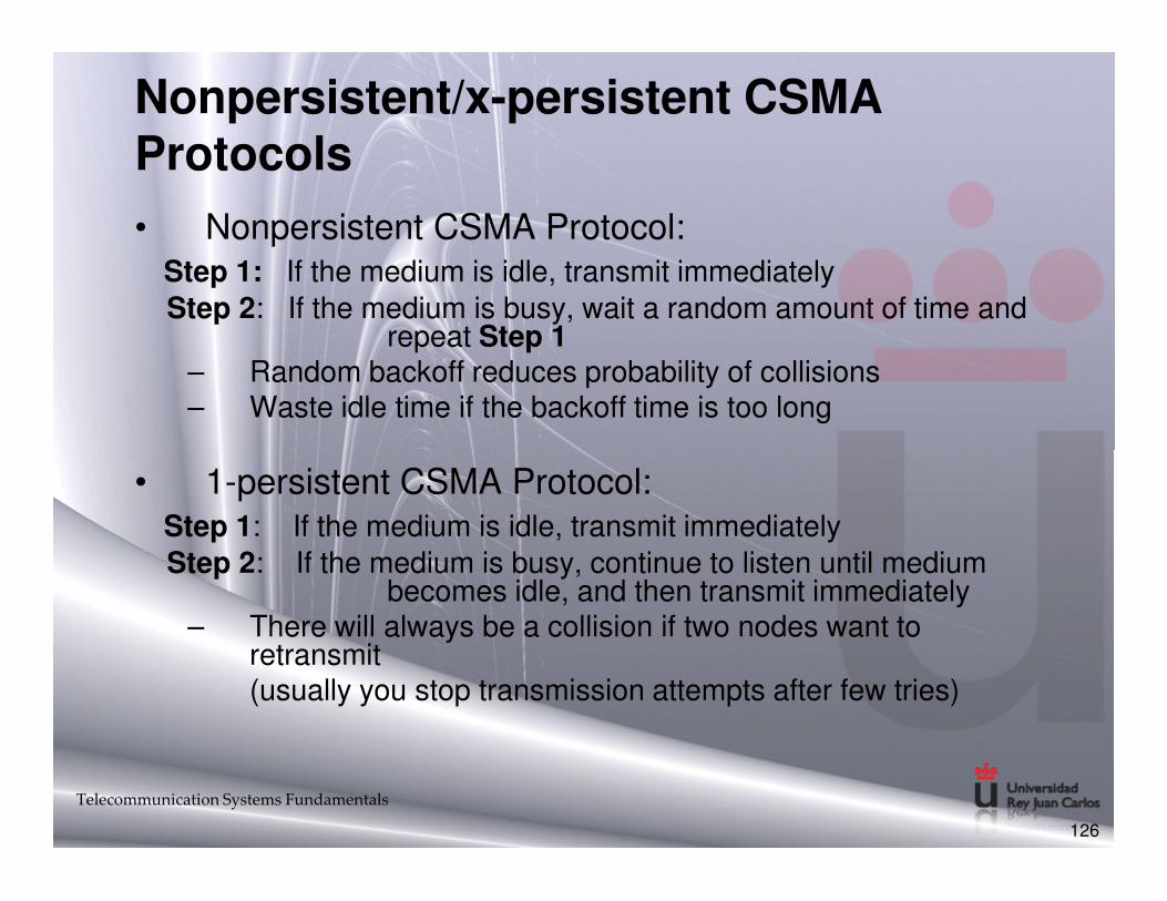
Nonpersistent/x-persistent CSMA Protocols
• Nonpersistent CSMA Protocol:Step 1: If the medium is idle, transmit immediatelyStep 2: If the medium is busy, wait a random amount of time and
repeat Step 1– Random backoff reduces probability of collisions– Waste idle time if the backoff time is too long
• 1-persistent CSMA Protocol:Step 1: If the medium is idle, transmit immediatelyStep 2: If the medium is busy, continue to listen until medium
becomes idle, and then transmit immediately– There will always be a collision if two nodes want to
retransmit(usually you stop transmission attempts after few tries)
126
Telecommunication Systems Fundamentals

Nonpersistent/x-persistent CSMA Protocols
• p-persistent CSMA Protocol:Step 1: If the medium is idle, transmit with probability p, and delay for worst case propagation delay for one packet with probability (1-p)Step 2: If the medium is busy, continue to listen until medium becomes idle, then go to Step 1Step 3: If transmission is delayed by one time slot, continue with Step 1Step 1
– A good tradeoff between nonpersistent and 1-persistent CSMA
127
Telecommunication Systems Fundamentals
How to Select Probability p ?
• Assume that N nodes have a packet to send and the medium is busy
• Then, Np is the expected number of nodes that will attempt to transmit once the medium becomes idle
• If Np > 1, then a collision is expected to occur
Therefore, network must make sure that Np < 1 to avoid collision, where N is the maximum number of nodes that can be active at a time
128
Telecommunication Systems Fundamentals

Contention Protocols
• Throughput
1.0
0.9
0.8
0.70.1-persistent CSMA
0.01-persistent CSMA
Nonpersistent CSMA
129
0 1 2 3 4 5 6 7 8 9G
0.6
0.5
0.4
0.3
0.2
0.1
0
S
Aloha
Slotted Aloha
1-persistent CSMA
0.5-persistent CSMA
0.1-persistent CSMA
Telecommunication Systems Fundamentals
CSMA/CD (CSMA with Collision Detection)
• In CSMA, if 2 terminals begin sending packet at the same time, each will transmit its complete packet (although collision is taking place).
• Wasting medium for an entire packet time.
• CSMA/CD
Step 1: If the medium is idle, transmit
Step 2: If the medium is busy, continue to listen until the channel is idle then transmit
Step 3: If a collision is detected during transmission, cease transmitting
Step 4: Wait a random amount of time and repeats the same algorithm
130
Telecommunication Systems Fundamentals
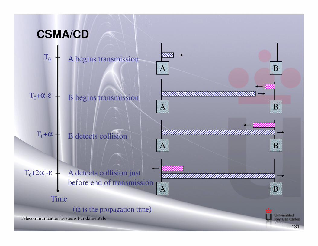
CSMA/CD
A B
T0 A begins transmission
A BB begins transmissionT0+α-ε
131
(α is the propagation time)
Time
A BB detects collisionT0+α
A B
A detects collision just before end of transmission
T0+2α -ε
Telecommunication Systems Fundamentals
CSMA/CA (CSMA with collision Avoidance)
• All terminals listen to the same medium as CSMA/CD
• Terminal ready to transmit senses the medium
• If medium is busy it waits until the end of current transmission
• It again waits for an additional predetermined time period DIFS (Distributed inter frame Space)
• Then picks up a random number of slots (the initial value of backoff counter) within a contention window to wait before backoff counter) within a contention window to wait before transmitting its frame
• If there are transmissions by other terminals during this time period (backoff time), the terminal freezes its counter
• It resumes count down after other terminals finish transmission + DIFS. The terminal can start its transmission when the counter reaches to zero
132
Telecommunication Systems Fundamentals

CSMA/CA
Time
Node A’s frame
Nodes B & C sense the medium
Node B’s frame
Delay: BDelay: C
Node C’s frame
133
the medium
Nodes B resenses the medium and transmits its frame.
Node C freezes its counter.
Nodes C starts transmitting.
Nodes C resenses the medium and starts
decrementing its counter.
Telecommunication Systems Fundamentals
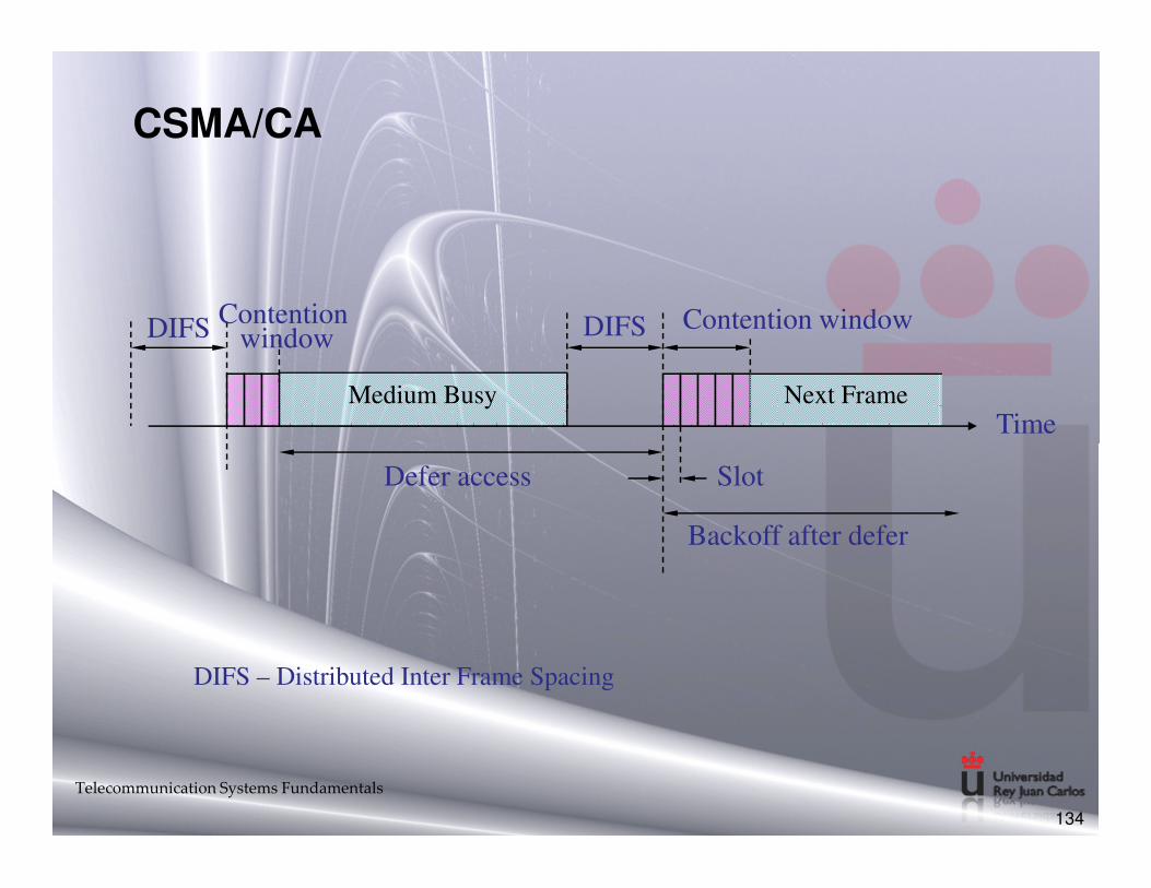
CSMA/CA
DIFS
Next FrameMedium Busy
DIFS Contention window
Time
Contentionwindow
134
Defer access
Backoff after defer
Slot
DIFS – Distributed Inter Frame Spacing
Telecommunication Systems Fundamentals
CSMA/CA with ACK
• Immediate Acknowledgements from receiver upon reception of data frame without any need for sensing the medium.
• ACK frame transmitted after time interval SIFS (Short Inter-Frame Space) (SIFS < DIFS)
• Receiver transmits ACK without sensing the medium.• Receiver transmits ACK without sensing the medium.
• If ACK is lost, retransmission done.
135
Telecommunication Systems Fundamentals
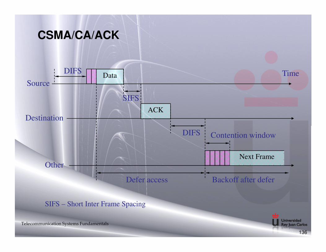
CSMA/CA/ACK
DIFS
ACK
DataSource
Destination
SIFS
Time
136
Next FrameOther
DIFS Contention window
Defer access Backoff after defer
SIFS – Short Inter Frame Spacing
Telecommunication Systems Fundamentals
CSMA/CA with RTS/CTS
• Transmitter sends an RTS (request to send) after medium has been idle for time interval more than DIFS.
• Receiver responds with CTS (clear to send) after medium has been idle for SIFS.
• Then Data is exchanged.• Then Data is exchanged.
• RTS/CTS is used for reserving channel for data transmission so that the collision can only occur in control message.
137
Telecommunication Systems Fundamentals
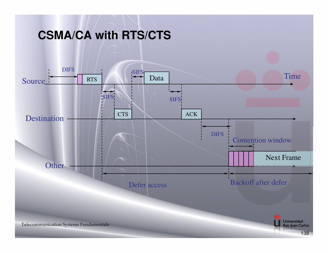
CSMA/CA with RTS/CTS
DIFS
CTS
RTSSource
Destination
SIFS
SIFSData
SIFS
ACK
Time
138
Next FrameOther
DIFS Contention window
Defer access Backoff after defer
Telecommunication Systems Fundamentals
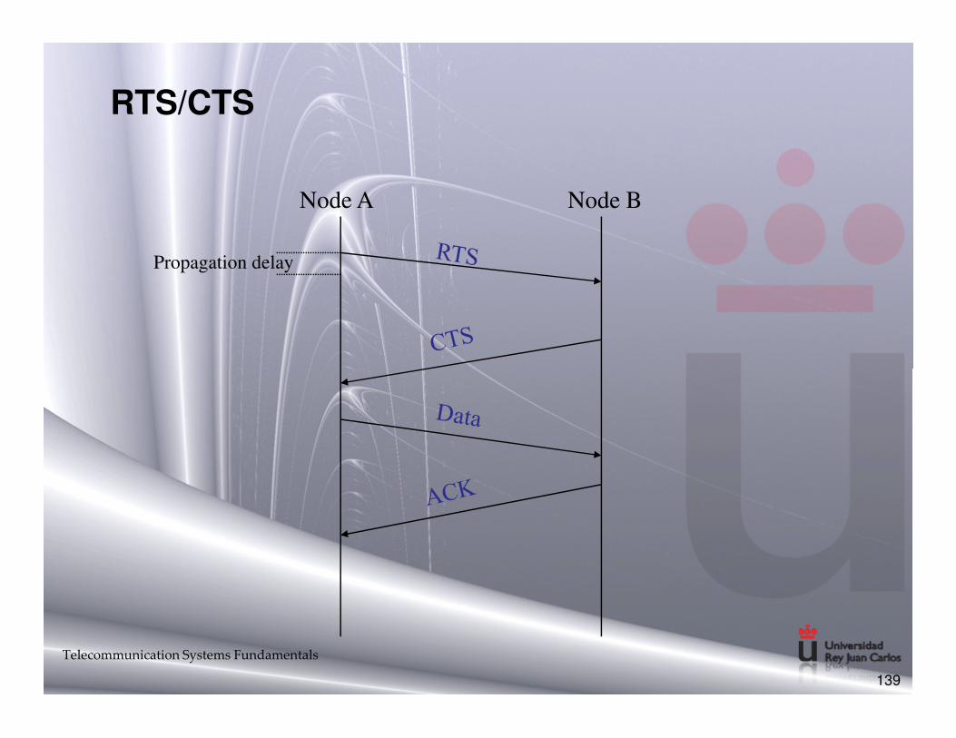
RTS/CTS
Node A Node B
Propagation delay
139
Telecommunication Systems Fundamentals

Summary of Concepts in this Chapter
• What are Logarithmic Units (dB) and the advantages we get by using them
• Whow we measure the Quality of the Service in data transmission
• Advantages and drawbacks of digital transmission
• Fundamentals of Communications networks topologies • Fundamentals of Communications networks topologies and technologies
• Main functionalities (blocks) of Analog Communications
• Main functionalities (blocks) of Digital Communications
• Multiplexing and Multiple Access
Telecommunication Systems Fundamentals
140
Related Documents