Topic 3: Traffic Network Equilibrium

Topic 3: Traffic Network Equilibrium

Professor Anna Nagurney

John F. Smith Memorial Professorand

Director – Virtual Center for SupernetworksIsenberg School of Management

University of MassachusettsAmherst, Massachusetts 01003

SCH-MGMT 825Management Science Seminar

Variational Inequalities, Networks, and Game TheorySpring 2014c©Anna Nagurney 2014

Professor Anna Nagurney SCH-MGMT 825 Management Science Seminar

Traffic Network Equilibrium

The problem of users of a congested transportation networkseeking to determine their travel paths of minimal cost from originsto their respective destinations is a classical network equilibriumproblem.

It appears as early as 1920 in the work of Pigou, who considered atwo-node, two-link (or path) transportation network, and wasfurther developed by Knight (1924).



The problem has an interpretation as an economic equilibriumproblem where the demand side corresponds to potential travelers,or consumers, of the network, whereas the supply side isrepresented by the network itself, with prices corresponding totravel costs.

The equilibrium occurs when the number of trips between anorigin and a destination equals the travel demand given bythe market price, that is, the travel time for the trips.


Wardrop’s Principles of Traffic

Wardrop (1952) stated the traffic equilibrium conditions throughtwo principles:

First Principle: The journey times of all routes actually used areequal, and less than those which would be experienced by a singlevehicle on any unused route.

Second Principle: The average journey time is minimal.

The first principle is referred to as user-optimization whereas thesecond is referred to as system-optimization.



Beckmann, McGuire, and Winsten (1956) were the first torigorously formulate these conditions mathematically, as hadSamuelson (1952) in the framework of spatial price equilibriumproblems in which there were, however, no congestion effects.

In particular, Beckmann, McGuire, and Winsten (1956) establishedthe equivalence between the equilibrium conditions and theKuhn-Tucker conditions of an appropriately constructedoptimization problem, under a symmetry assumption on theunderlying functions. Hence, in this case, the equilibrium link andpath flows could be obtained as the solution of a mathematicalprogramming problem.


Celebrating to 50th anniversary of the publication of Studies inthe Economics of Transportation, by Beckann, McGuire, andWinsten at the INFORMS San Francisco meeting on November 14,2005.


Traffic Network Equilibrium Models - Multimodal

Consider now a transportation network. Let a, b, c , etc., denotethe links; p, q, etc., the paths. Assume that there are J O/D pairs,with a typical O/D pair denoted by w , and k modes oftransportation on the network with typical modes denoted by i , j ,etc. G denotes the graph G = [N, L], where N is the set of nodesand L the set of links. P denotes the set of paths.


The Link Cost Structure

The flow on a link a generated by mode i is denoted by f ia , and the

user cost associated with traveling by mode i on link a is denotedby c i

a. Group the link flows into a column vector f ∈ RknL , wherenL is the number of links in the network. Group the link costs intoa row vector c ∈ RknL . Assume now that the user cost on a linkand a particular mode may, in general, depend upon the flows ofevery mode on every link in the network, that is,

c = c(f ), (1)

where c is a known smooth function.


The Travel Demands and O/D Pair Travel Disutilities

The travel demand of potential users of mode i traveling betweenO/D pair w is denoted by d i

w and the travel disutility associatedwith traveling between this O/D pair using the mode is denoted byλi

w . Group the demands into a vector d ∈ RkJ and the traveldisutilities into a vector λ ∈ RkJ .

The flow on path p due to mode i is denoted by x ip. Group the

path flows into a column vector x ∈ RknP , where nP denotes thenumber of paths in the network.


Conservation of Flow Equations

The conservation of flows equations are as follows. The demandfor a mode and O/D pair must be equal to the sum of the flows ofthe mode on the paths joining the O/D pair, that is,

d iw =

∑p∈Pw

x ip, ∀i ,w (2)

where Pw denotes the set of paths connecting w .

A nonnegative path flow vector x which satisfies (2) is termedfeasible. Moreover, we must have that

f ia =

∑p∈P

x ipδap, (3)

that is, that the flow on a link from a mode is equal to the sum ofthe flows of that mode on all paths that contain that link.


Traffic Network Equilibrium Condition - Elastic Demand

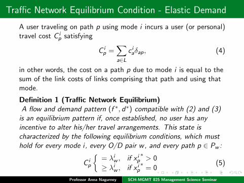
A user traveling on path p using mode i incurs a user (or personal)travel cost C i

p satisfying

C ip =

∑a∈L

c iaδap, (4)

in other words, the cost on a path p due to mode i is equal to thesum of the link costs of links comprising that path and using thatmode.

Definition 1 (Traffic Network Equilibrium)A flow and demand pattern (f ∗, d∗) compatible with (2) and (3)

is an equilibrium pattern if, once established, no user has anyincentive to alter his/her travel arrangements. This state ischaracterized by the following equilibrium conditions, which musthold for every mode i , every O/D pair w, and every path p ∈ Pw :

C ip

{= λi

w , if x ip∗> 0

≥ λiw , if x i

p∗

= 0(5)

where λiw is the equilibrium travel disutility associated with the

O/D pair w and mode i .


The Elastic Demand Model with Disutility Functions

Assume that there exist travel disutility functions, such that

λ = λ(d), (6)

where λ is a known smooth function. That is, let the traveldisutility associated with a mode and an O/D pair depend, ingeneral, upon the entire demand pattern.

Let K denote the feasible set defined by

K = {(f , d) |∃ x ≥ 0 | (2) , (3) hold}. (7)

The variational inequality formulation of the equilibrium conditions(5) is given in the next theorem. Assume that λ is a row vectorand d is a column vector.


Theorem 1 (Variational Inequality Formulation)A pair of vectors (f ∗, d∗) ∈ K is an equilibrium pattern if and onlyif it satisfies the variational inequality problem

c(f ∗) · (f − f ∗)− λ(d∗) · (d − d∗) ≥ 0, ∀(f , d) ∈ K . (8)

Proof: Note that equilibrium conditions (5) imply that[C i

p(f∗)− λi

w (d∗)]×

[x ip − x i

p∗] ≥ 0, (9)

for any nonnegative x ip. Indeed, if x i

p∗> 0, then[

C ip(f

∗)− λiw (d∗)

]= 0,

and (9) holds; whereas, if x ip∗

= 0, then[C i

p(f∗)− λi

w (d∗)]≥ 0,

and since x ip ≥ 0, (9) also holds.


Observe that (9) holds for each path p ∈ Pw ; hence, one may write∑p∈Pw

[C i

p(f∗)− λi

w (d∗)]×

[x ip − x i

p∗] ≥ 0, (10)

and, in view of constraint (2), (10) may be rewritten as:∑p∈Pw

C ip(f

∗)× (x ip − x i

p∗)− λi

w (d∗)× (d iw − d i

w∗) ≥ 0. (11)

But (11) holds for each mode i and every O/D pair w , hence, oneobtains:∑

i ,w

C ip(f

∗)× (x ip − x i

p∗)−

∑i ,w

λw (d∗)× (d iw − d i

w∗) ≥ 0. (12)

In view of (3) and (4), (12) is equivalent to: For (f ∗, d∗) ∈ K ,induced by a feasible x∗:∑

i ,a

c ia(f

∗)× (f ia − f i

a∗)−

∑i ,w

λiw (d∗)× (d i

w − d iw∗) ≥ 0,

∀(f , d) ∈ K , (13)

which, in vector form, yields (8).Professor Anna Nagurney SCH-MGMT 825 Management Science Seminar

We now establish that (f ∗, d∗) ∈ K , induced by a feasible x∗ andsatisfying variational inequality (8) (i.e., (12)), also satisfiesequilibrium conditions (5). Fix any mode i , and any path p thatjoins an O/D pair w . Construct a feasible flow x such that

x jq = x j

q∗

(j , q) 6= (i , p), but x ip 6= x i

p∗. Then d j

v∗

= d jv ,

(j , v) 6= (i ,w), but d iw = d i

w∗+ x i

p − x ip∗. Upon substitution into

(12) one obtains

C ip(f

∗)× (x ip − x i

p∗)− λi

w (d∗)× (d iw − d i

w∗) ≥ 0. (14)

Now, if x ip∗> 0, one may select x i

p such that x ip > x i

p∗

or x ip < x i

p∗,

and, consequently, (14) will hold only if[C i

p(f∗)− λi

w (d∗)]

= 0.

On the other hand, if x ip∗

= 0, then x ip ≥ x i

p∗, so that (13) yields

C ip(f

∗) ≥ λiw (d∗),

and the proof is complete.


Qualitative Properties of the Model

Observe that in the above model the feasible set is not compact.Therefore, a condition such as strong monotonicity wouldguarantee both existence and uniqueness of the equilibrium pattern(f ∗, d∗); in other words, if one has that[

c(f 1)− c(f 2)]·[f 2 − f 2

]−

[λ(d1)− λ(d2)

]·[d1 − d2

]≥ α(‖f 1 − f 2‖2 − ‖d1 − d2‖2), ∀(f 1, d1), (f 2, d2) ∈ K , (15)

where α > 0 is a constant, then there is only one equilibriumpattern.



Condition (15) implies that the user cost function on a link due toa particular mode should depend primarily upon the flow of thatmode on that link; similarly, the travel disutility associated with amode and an O/D pair should depend primarily on that mode andthat O/D pair. The link cost functions should be monotonicallyincreasing functions of the flow and the travel disutility functionsmonotonically decreasing functions of the demand.


The Elastic Demand Model with Demand Functions

We assume that there exist travel demand functions, such that

d = d(λ) (16)

where d is a known smooth function. Assume here that d is a rowvector. In this case, the variational inequality formulation ofequilibrium conditions (5) is given in the subsequent theorem,whose proof appears in Dafermos and Nagurney (1984a).

Theorem 2 (Variational Inequality Formulation)Let M denote the feasible set defined by

M = {(f , d , λ)|λ ≥ 0,∃ x ≥ 0 | (2), (3) hold}. (17)

The vector X ∗ = (f ∗, d∗, λ∗) ∈M is an equilibrium pattern if andonly if it satisfies the variational inequality problem:

F (X ∗) · (X − X ∗) ≥ 0, ∀X ∈M, (18)

where F : M 7→ Rk(nL+2J) is the function defined by

F (f , d , λ) = (c(f ),−λT , d − d(λ)). (19)Professor Anna Nagurney SCH-MGMT 825 Management Science Seminar


To obtain existence one could impose either a strong monotonicitycondition or coercivity condition on the functions c and d .

However, strong monotonicity (or coercivity), although reasonablefor c , may not be a reasonable assumption for d . The followingtheorem provides a condition under which the existence of asolution to variational inequality (18) is guaranteed under a weakercondition.



Theorem 3 (Existence)Let c and d be given continuous functions with the followingproperties: There exist positive numbers k1 and k2 such that

c ia(f ) ≥ k1, ∀a, i and f ∈M (20)

andd iw (λ) < k2, ∀w , λ with λi

w ≥ k2. (21)

Then (18) has at least one solution.



As in the model with known travel disutility functions, thedifficulty of showing existence of a solution for variationalinequality (18) is that the feasible set is unbounded.

This difficulty can be circumvented as follows. Observe that due tothe special structure of the problem, no equilibrium may exist withvery large travel demands because such demands would contradictassumption (21), in view of (16).

A bounded vector d , in turn, would imply that f is also bounded.This would then imply that c(f ) is bounded and, therefore, λ isbounded by virtue of (5) and (1). Consequently, one expects thatimposing constants of the type d ≤ η and λ ≤ V , for η and Vsufficiently large, will not affect the set of solutions of (18), whilerendering the set compact. We now present a proof through thesubsequent two lemmas.



First, fixV >

∑f ib≤k2J

max c ia(f ) (22)

and consider the compact, convex set

L = {(f , d , λ)| 0 ≤ λ ≤ V ; 0 ≤ d ≤ k2; ∃x ≥ 0| (2), (3) hold}.(23)

Consider the variational inequality problem:

Determine X ∗ ∈ L, such that

F (X ∗) · (y − X ∗) ≥ 0, ∀y ∈ L. (24)

Since F is continuous and L is compact, there exists at least onesolution, say, X ∗ = (f ∗, d∗, λ∗) to (24). The claim is that X ∗ isactually a solution to the original variational inequality (18).



Lemma 1If X ∗ = (f ∗, d∗, λ∗) is any solution of variational inequality (24),then

d iw∗< k2, ∀i ,w (25)

λiw∗< V , ∀i ,w . (26)

Lemma 2Let X ∗ = (f ∗, d∗, λ∗) be a solution of variational inequality (24).Suppose that

d iw∗< k2, ∀w , i (27)

λiw∗< V , ∀w , i . (28)

Then X ∗ is a solution to the original variational inequality (18).



Using similar arguments one may establish existence conditions forthe model in which travel disutility functions are assumed given,that is, one has the following result.

Theorem 4 (Existence)Let c and λ be given continuous functions with the followingproperties: There exist positive numbers k1 and k2 such that

c ia(f ) ≥ k1, ∀a, i and f ∈ K

andλi

w (d) < k1, ∀w , i and d with d iw ≥ k2.

Then variational inequality (8) has at least one solution.


The Fixed Demand Model

We now present the fixed demand model is presented is thissection. Specifically, it is assumed that the demand d i

w is now fixedand known for all modes i and all origin/destination pairs w . Inthis case, the feasible set K would be defined by

K = {f | ∃ x ≥ 0 | (2), (3) hold}. (29)

The variational inequality governing equilibrium conditions (5) forthis model would be given as in the subsequent theorem. Smith(1979) stated the traffic equilibrium conditions thus whereasDafermos (1980) identified the formulation as being that of afinite-dimensional variational inequality problem.


The Fixed Demand Model

Theorem 5 (Variational Inequality Formulation)A vector f ∗ ∈ K, is an equilibrium pattern if and only if it satisfiesthe variational inequality problem

c(f ∗) · (f − f ∗) ≥ 0, ∀f ∈ K . (30)


Qualitative Properties

Existence of an equilibrium f ∗ follows from the standard theory ofvariational inequalities solely from the assumption that c iscontinuous, since the feasible set K is now compact.

In the special case where the symmetry condition[∂c i

a

∂f jb

=∂c j

b

∂f ia

], ∀i , j ; a, b

holds, then the variational inequality problem (30) is equivalent tosolving the optimization problem:

Minimizef ∈K

∑a,i

∫ f ia

0c ia(x)dx . (31)


Qualitative Properties

This symmetry assumption, however, is not expected to hold inmost applications, and thus the variational inequality problemwhich is the more general problem formulation is needed.

For example, the symmetry condition essentially says that the flowon link b due to mode j should affect the cost of mode i on link ain the same manner that the flow of mode i on link a affects thecost on link b and mode j . In the case of a single mode problem,the symmetry condition would imply that the cost on link a isaffected by the flow on link b in the same manner as the cost onlink b is affected by the flow on link a.


Variations of the Model

In the above framework, with the appropriate construction of therepresentative network, one can also handle the followingsituations.

Situation 1: Users of the network have predetermined origins, butare free to select their destinations as well as their travel paths.

Situation 2: Users of the network have predetermineddestinations, but they are free to select their origins as well as theirtravel paths.

Situation 3: Users of the network are free to select their origins,their destinations, as well as their travel paths.


Variations of the Model

The above situations lead, respectively, to the following networkequilibrium problems.

Problem 1: The total number O iu of trips produced in each origin

node u by each mode (or class) i is given. Determine the O/Dtravel demands and the equilibrium flow pattern.

Problem 2: The total number D iv of trips attracted to each

destination node v by each mode i is given. Determine the O/Dtravel demands and the equilibrium flow pattern.

Problem 3: The total number T i of trips generated in all originnodes by all modes i of the network are given, which is equal tothe total number of trips attracted to all destinations by eachmode. Determine the trip productions O i

u, the trip attractions D iv ,

the O/D travel demands, and the equilibrium flow pattern.


Comments

Here, of course, travel cost should be interpreted liberally. Abovewe assume that each user of the network, subject to theconstraints, chooses his/her origin, and/or destination, and path,so as to minimize his/her travel cost given that all other users havemade their choices.

The additional factors of attractiveness of the origins and thedestinations are taken into account by being incorporated into themodel as “travel costs” by a modification of the network throughthe addition of artificial links with travel cost representingattractiveness.


Comments

For example, in Problem 1, we can modify the original network byadding artificial nodes ψi , for each mode i , and joining everydestination node v of the original network with ψi by an artificiallink (v , ψi ). We assume that the travel cost over the artificial linksis zero.

It is easy to verify that in computing the equilibrium flowsaccording to equilibrium conditions (5) on the expanded network,one can recover the equilibrium flows for the original network. Onecan make analogous constructions for Problems 2 and 3.


Stability and Sensitivity Analysis

In 1968, Braess presented an example in which the addition of anew link to a network, which resulted in a new path, actually madeall the travelers in the network worse off in that the travel cost ofall the users was increased. This example, which came to beknown as Braess’s paradox, generated much interest in addressingquestions of stability and sensitivity of traffic network equilibria.


Professor Braess’s visit to UMass, Spring 2006

http://supernet.isenberg.umass.edu/cfoto/braess-visit/braessvisit.html


http://supernet.isenberg.umass.edu/cfoto/braess-visit/braessvisit.html

The Braess Paradox

The Braess Paradox Illustrates Why

Capturing the Behavior of Users on Networks

is Essential


The Braess (1968) Paradox

Assume a network with a singleO/D pair w1 = (1, 4). There are2 paths available to travelers:p1 = (a, c) and p2 = (b, d).

For a travel demand dw of 6, theU-O / equilibrium path flows are:x∗p1

= x∗p2= 3 and

the U-O / equilibrium pathtravel costs are:Cp1 = Cp2 = 83.

� ��4

� ��2

@@

@@@R

c

� ��3

��

��

�

d

� ��1

��

��

�

a

@@

@@@R

b

ca(fa) = 10fa, cb(fb) = fb + 50,

cc(fc) = fc +50, cd(fd) = 10fd .


Adding a Link Increases Travel Cost for All!

Adding a new link e creates anew path p3 = (a, e, d). The userlink cost on e is: ce(fe) = fe + 10and dw1 remains at 6.The original flow distributionpattern is no longer a U-Opattern, since, at that level offlow, the cost on pathp3,Cp3 = 70.

The new U-O flow pattern isx∗p1

= x∗p2= x∗p3

= 2.The U-O path travel costs arenow: Cp1 = Cp2 = Cp3 = 92.

The travel cost has increasedfor all from 83 to 92!

� ��4

� ��2

@@

@@@R

c

� ��3

��

��

�

d

-e

ce(fe) = fe + 10

� ��1

��

��

�

a

@@

@@@R

b


Under S-O behavior, the total cost in thenetwork is minimized, and the new route p3,under the same demand of 6, would not beused.

The Braess paradox never occurs in S-Onetworks and only in U-O networks!


The Braess Paradox Around the World

1969 - Stuttgart, Germany -The traffic worsened until anewly built road was closed.

1990 - Earth Day - New YorkCity - 42nd Street was closedand traffic flow improved.

2002 - Seoul, Korea - A 6 laneroad built over theCheonggyecheon River thatcarried 160,000 cars per day andwas perpetually jammed was torndown to improve traffic flow.


The Closing of Broadway in NYC to Traffic from 42nd to47th Streets in 2009 Until Now

In May 2009, Mayor Bloomberg’s administrationimplemented the closing of Broadway from 42nd Street(Times Square) to 47th Street to traffic and the creation ofpedestrian plazas. This closure generated much discussion andwas the subject of, among others, the World Science FestivalTraffic panel in NYC in June 2009.

World Science Festival Traffic panel in NYC in June 2009



Interview on Broadway for America Revealed on March 15,2011

http://video.pbs.org/video/2192347741/Professor Anna Nagurney SCH-MGMT 825 Management Science Seminar

http://video.pbs.org/video/2192347741/

� ��4

� ��2

@@

@@@R

c

� ��3

��

��

�

d

-e

� ��1

��

��

�

a

@@

@@@R

b

Recall the Braess network with the added link e.

What happens as the demand increases?


The U-O Solution of the Braess Network with Added Link (Path)and Time-Varying Demands Solved as an Evolutionary VariationalInequality (Nagurney, Daniele, and Parkes (2007)).


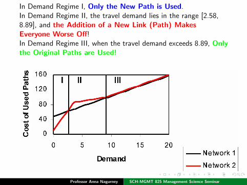
In Demand Regime I, Only the New Path is Used.In Demand Regime II, the travel demand lies in the range [2.58,8.89], and the Addition of a New Link (Path) MakesEveryone Worse Off!In Demand Regime III, when the travel demand exceeds 8.89, Onlythe Original Paths are Used!


The new path is never used, under U-Obehavior, when the demand exceeds 8.89,even out to infinity!


Basic Sensitivity Analysis

Note:

The addition of a new path on a network may: increase,decrease, or leave unchanged the equilibrium (U-O) travelpath costs.

In the case of S-O solution, the addition of a new path cannever increase the total system cost in the network.

Hence, from the system point of view, the network is“improved” or at least not worsened.



Question:

Can you design a new path connecting O/D pair w1 in theoriginal Braess paradox network so that the travelers cannever be worse off, from a U-O perspective?



What can we say about the effect on users’, that is,travelers’, costs with respect to:

� an increase in travel demand?

� a decrease in travel demand?

� an increase in the link cost function?

� a decrease in the link cost function?


Stability Results for the Models

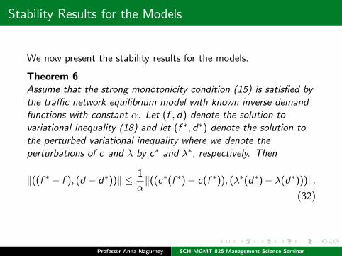
We now present the stability results for the models.

Theorem 6Assume that the strong monotonicity condition (15) is satisfied bythe traffic network equilibrium model with known inverse demandfunctions with constant α. Let (f , d) denote the solution tovariational inequality (18) and let (f ∗, d∗) denote the solution tothe perturbed variational inequality where we denote theperturbations of c and λ by c∗ and λ∗, respectively. Then

‖((f ∗ − f ), (d − d∗))‖ ≤ 1

α‖((c∗(f ∗)− c(f ∗)), (λ∗(d∗)− λ(d∗)))‖.

(32)



Theorem 7Assume that c(f ) is strongly monotone with constant α and that fsatisfies variational inequality (30). Let f ∗ denote the solution tothe perturbed variational inequality with perturbed cost vector c∗.Then

‖f ∗ − f ‖ ≤ 1

α‖c∗(f ∗)− c(f ∗)‖. (33)



In order to attempt to further illuminate paradoxical phenomena intransportation networks, the sensitivity analysis results arepresented for the fixed demand model.

Theorem 8Assume that f ∈ K satisfies variational inequality (30) and thatf ∗ ∈ K is the solution to the perturbed variational inequality withperturbed cost vector c∗. Then

[c∗(f ∗)− c(f )] · [f ∗ − f ] ≤ 0. (34)

Inequality (34) may be interpreted as follows: Although animprovement in the cost structure of a network may result in anincrease of some of the incurred costs and a decrease in some ofthe flows, a certain total average cost in the network may beviewed as nonincreasing.


Toll Policies

We now describe how tolls, either in the form of path tolls or linktolls, can be imposed in order to make the system-optimizingsolution also user-optimizing. Tolls serve as a mechanism formodifying the travel cost as perceived by the individualtravelers. We shall show that in the path-toll collection policythere is a degree of freedom that is not available in the link-tollcollection policy and how one can take advantage of this addeddegree of freedom. The analysis is conducted for the trafficnetwork equilibrium model with fixed travel demands.


Toll Policies

Recall that the system-optimizing flow pattern is one thatminimizes the total travel cost over the entire network, whereas theuser-optimized flow pattern has the property that no user has anyincentive to make a unilateral decision to alter his/her travel path.

One would expect the former pattern to be established when acentral authority dictates the paths to be selected, so as tominimize the total cost in the system, and the latter, whentravelers are free to select their routes of travel so as to minimizetheir individual travel cost.

The latter solution, however, results in a higher total system costand, in a sense, is an underutilization of the transportationnetwork. In order to remedy this situation tolls can be applied withthe recognition that imposing tolls will not change the travel costas perceived by society since tolls are not lost.


Toll Policies

In particular, in this section it shall be shown how tolls can becollected on a link basis, that is, every member of a class (ormode) on a link will be charged the same toll, irrespective of originor final destination, or on a path basis, in which every member of aclass traveling from an origin to a destination on a particular pathwill be charged the same toll.

In the link-toll collection policy a toll r ia is associated with each link

a and mode i . In the path-toll collection policy a toll r ip is

associated with each path p and mode i .

Of course, even in the link-toll collection policy one may define a“path toll” for class i through the expression

r ip =

∑a∈L

r iaδap. (35)


Toll Policies

Observe that after the imposition of tolls the travel cost asperceived by society remains c i

a(f ), for all links a and all modes i .The travel cost as perceived by the individual, however, is modifiedto

C ip = C i

p(f ) + r ip, ∀p, i . (36)

Consequently, a system-optimizing flow pattern is still defined asbefore, that is, it is one that solves the problem

Minimizef ∈K

∑a,i

c ia(f ) (37)

where c ia(f ) = c i

a(f )× f ia .


Toll Policies

In particular, the solution to (37), under the assumption that eachc ia(f ) is convex, is equivalent to the following statement: For every

O/D pair w , and every mode i , there exists an ordering of thepaths p ∈ Pw , such that

C i ′p1

(f ) = . . . = C i ′psi

(f ) = µiw ≤ C i ′

psi+1(f ) ≤ . . . ≤ C i ′

pmw(38)

x ipri> 0, ri = 1, . . . , si

x ipri

= 0, ri = si+1, . . . ,mw ,

where mw denotes the number of paths for O/D pair w . Here weuse the notation

C i ′p =

∑j

∑a,b

∂cbj(f )

∂f ia

δap. (39)


Toll Policies

On the other hand, in view of equilibrium conditions (5) one candeduce that the system-optimizing flow pattern x , after theimposition of a toll policy, is at the same time user-optimizing if:For every O/D pair w , every path p ∈ Pw , and every mode i :

C ip1

(f ) = . . . = C ipsi

(f ) = λiw ≤ C i

psi +1(f ) ≤ . . . ≤ C i

pmw(f ) (40)

x ipri> 0, ri = 1, . . . , si

x ipri

= 0, ri = si+1, . . . ,mw .


Toll Policies

We now state:

Proposition 1A toll-collection policy renders a system-optimizing flow patternuser-optimizing if and only if for each mode i , and O/D pair w

r ip1

= λiw − C i

p1(f )

...... (41)

r ipsi

= λiw − C i

psi(f )

r ipsi+1

≥ λiw − C 1

psi+1(f )

......

r ipmw

≥ λiw − C i

pmw(f ). (42)


Toll Policies

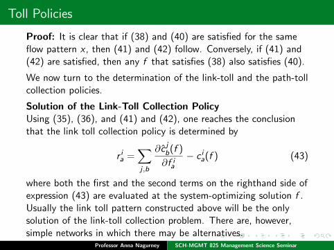
Proof: It is clear that if (38) and (40) are satisfied for the sameflow pattern x , then (41) and (42) follow. Conversely, if (41) and(42) are satisfied, then any f that satisfies (38) also satisfies (40).

We now turn to the determination of the link-toll and the path-tollcollection policies.

Solution of the Link-Toll Collection PolicyUsing (35), (36), and (41) and (42), one reaches the conclusionthat the link toll collection policy is determined by

r ia =

∑j ,b

∂c jb(f )

∂f ia

− c ia(f ) (43)

where both the first and the second terms on the righthand side ofexpression (43) are evaluated at the system-optimizing solution f .Usually the link toll pattern constructed above will be the onlysolution of the link-toll collection problem. There are, however,simple networks in which there may be alternatives.


Toll Policies

Hence, to determine an appropriate toll policy, one first mustcompute the system-optimizing solution.

This can be accomplished using a general-purpose convexprogramming algorithm, an appropriate nonlinear network code, or,in the case of separable linear user cost functions, an equilibrationalgorithm. Once the system-optimizing solution is established, onethen substitutes that flow pattern f into equation (43) to computethe link toll r i

a for all links a and all modes (or classes) i .


Solution of the Path-Toll Collection Policy

It is obvious from (41) and (42) that one may construct an infinitenumber of solutions of the path-toll collection problem. Forexample, one may select, a priori, for each class w , the level ofpersonal travel cost λi

w , as well as the values of r ipsi+1

, . . . , r ipmw

,

subject to only constraint (42), and then determine a path tollpattern according to (41). Hence, in this case there is someflexibility in selecting a toll pattern, and one can incorporateadditional objectives. Certain possibilities are:


Solution of the Path-Toll Collection Policy

(i) One may wish to ensure that some, if not all, classes oftravelers are charged with a nonnegative toll; in other words, nosubsidization is allowed for these classes. This can be accomplishedby choosing the corresponding λi

w sufficiently large.

(ii) Suppose one wishes a “fair” policy. A possible one would be toensure that the level of personal travel cost λi

w is equal to thepersonal travel cost λi

w before the imposition of tolls.


An Example

Consider the network depicted the figure in which there are threenodes: 1, 2, 3; three links: a,b,c; and a single O/D pairw1 = (1, 3). Let path p1 = (a, c) and path p2 = (b, c).

j

j

j

1

2

3?

a b

c

R

Figure: A link-toll policy example

Assume, for simplicity, the user cost functions:

ca(fa) = fa + 5 cb(fb) = 2fb + 10 cc(fc) = fc + 15,

and the travel demand:dw1 = 100.


An Example

We now turn to the computation of the link toll policy. It is easyto verify that the system-optimizing solution is:

xp1 = 67.5 xp2 = 32.5,

with associated link flow pattern:

fa = 67.5 fb = 32.5 fc = 100,

and with marginal path costs:

C ′p1

= C ′p2

= 355.

The link toll policy that renders this system-optimizing flowpattern also user-optimized is given by:

ra = 67.5 rb = 65 rc = 100,

with the induced user costs Cp1 = Cp2 = 355.


Computation of Traffic Network Equilibria

We now focus on the computation of traffic network equilibriumproblems. In particular, the elastic, multimodal model with knowntravel disutility functions is considered. The fixed demand modelcan be viewed as a special case, and the algorithms that will bedescribed here can be readily adapted for the solution of thismodel as well. Specifically, both the projection method and therelaxation method are presented for this problem domain.



Assume that the strong monotonicity condition (15) is satisfied.

The Projection Method

Step 0: Initialization

Select an initial feasible flow and demand pattern (f 0, d0)∈K .Also, select symmetric, positive definite matrices G and −M,where G is an knL × knL matrix and −M is an kJ × kJ matrix.Select ρ such that

0 < ρ < min

[2α

η,2α

µ

],

where α is constant in the strong monotonicity condition, and ηand µ are the maximum over K of the maximum of the positivedefinite symmetric matrices[

∂c

∂f

]T

G−1

[∂c

∂f

]and

[∂λ

∂d

]T

M−1

[∂λ

∂d

].

Set t := 1.Professor Anna Nagurney SCH-MGMT 825 Management Science Seminar


Step 1: Construction and Computation

Constructht−1 = ρc(f t−1)− Gf t−1 (44)

andT t−1 = ρλ(d t−1)−Md t−1. (45)

Compute the unique user-optimized traffic pattern (f t , d t)corresponding to travel cost and disutility functions of the specialform:

ct−1(f ) = Gf + ht−1 (46)

andλt−1(d) = Md + T t−1. (47)

Step 2: Convergence Verification

If |f t − f t−1| ≤ ε and if |d t − d t−1| ≤ ε with ε > 0, a prespecifiedtolerance, stop; otherwise, set t := t + 1, and go to Step 1.



Possibilities for the selection of the matrices G and −M are anydiagonal positive definite matrices of appropriate dimensions. Onecould also set G and M to the diagonal parts of the Jacobianmatrices

[∂c∂f

]and

[∂λ∂d

], evaluated at the initial feasible flow

pattern.

Observe that if one selects diagonal matrices then the abovesubproblems are decoupled by mode of transportation and eachsubproblem can be allocated to a distinct processor forcomputation.



Observe that the projection method constructs a series ofsymmetric user-optimized problems in which the link user costfunctions and the travel disutility functions are linear. Hence, eachof these subproblems can be converted into a quadraticprogramming problem. Moreover, the subproblems can be solvedusing equilibration algorithms.



Theorem 9Assume that the strong monotonicity condition (15) holds andthat ρ is constructed as above. Then, for any (f 0, d0) ∈ K, theprojection method converges to the solution (f ∗, d∗) of variationalinequality (8).



The relaxation method for the same model is now presented.

The Relaxation Method

Step 0: Initialization

Select an initial feasible traffic pattern (f 0, d0) ∈ K . Set t := 1.

Step 1: Construction and Computation

Construct new user cost functions:

c(i) = c(i)(ft−1(1) , . . . , f t−1

(i−1), fi , ft−1(i+1), . . . , f

t−1(nL)

) (48)

for each mode i , where the subscript i denotes the vector of termscorresponding to mode i .Construct new travel disutility functions:

λ(i) = λ(i)(dt−1(1) , . . . , d

t−1(i−1), di , d

t−1(i+1), . . . , d

t−1(k) ) (49)

for each mode i .Professor Anna Nagurney SCH-MGMT 825 Management Science Seminar


Compute the solution to the user-optimized problem with theabove travel cost and travel disutility functions for each mode i .

Step 2: Convergence VerificationSame as in Step 2 above in the Projection Method.

Observe that the subproblem encountered at each iteration of therelaxation method will, in general, be a nonlinear problem.Moreover, the above algorithm yields k decoupled subproblems,each of which can also be solved on a distinct processor.



We assume that the variational inequality corresponding to theequilibrium problem with user cost functions (48) and traveldisutility functions (49) has a unique solution, which can becomputed by a certain algorithm.

Theorem 10Assume that the functions c(i), λ(i); i = 1, . . . , k, satisfy themonotonicity property:[

c(i)(f′(1), . . . , f(i), . . . , f

′(n))− c(i)(f

′(1), . . . , f(i), . . . , f

′(n))

]·[f(i) − f(i)

]−

[λ(i)(d

′(1), . . . , d(i), . . . , d

′(n))− λ(i)(d

′(1), . . . , d(i), . . . , d

′(n))

]·[d(i) − d(i)

](50)

≥ α1‖f(i) − f(i)‖2 + α2‖d(i) − d(i)‖2,

∀(f(i), d(i)), (f(i), d(i)), (f′(i), d

′(i)) ∈ K ,

where α1, α2 are positive constants.Professor Anna Nagurney SCH-MGMT 825 Management Science Seminar


Also, if there exists a constant γ; 0 < γ < 1, such that

sup{∑

i ,j ;i 6=j

‖∂c(i)

∂f(j)‖2}

12 ≤ γα1 (51)

sup{∑

i ,j ;i 6=j

‖∂λ(i)

∂d(j)‖2}

12 ≤ γα2 (52)

for all (f(i), d(i)) ∈ K, then there is a unique solution (f ∗(i), d∗(i));

i = 1, . . . , n, to variational inequality (8), and for an arbitrary(f 0

(i), d0(i)) ∈ K; i = 1, . . . , n; (f k

(i), dk(i))→(f ∗(i), d

∗(i)); i = 1, . . . , n, as

k →∞, where (f ∗, d∗) satisfies variational inequality (8).



In the case of a single-modal problem, the user cost functions (48)would be separable, that is,

ca = ca(ft−11 , . . . , fa, f

t−1a+1 , . . . , f

t−1nL

), ∀a (53)

and the travel disutility functions would also be separable, that is,

λw = λw (d t−11 , . . . , dw , d

t−1w , . . . , d t−1

J ), ∀w , (54)

in which case the variational inequality problem at Step 1 wouldhave an equivalent optimization reformulation given by

Minimize∑a∈L

∫ fa

0ca(x)dx −

∑w

∫ dw

0λw (y)dy (55)

subject to (f , d) ∈ K .



The projection method and the relaxation method may alsobe used to compute the solution to the fixed demand model.

In this case, only the user cost functions at each iteration wouldneed to be constructed. Results of numerical testing of thesealgorithms can be found in Nagurney (1984, 1986). See alsoMahmassani and Mouskos (1988).


Summary

Here we have provided variational inequality formulations of bothelastic demand and fixed demand traffic network equilibriumproblems.

We emphasized the importance of capturing the behavior of userson congested networks from transportation to the Internet.

In addition, we discussed the Braess paradox, which continues tofascinate to this day!

Both qualitative analysis results were given along withcomputational procedures.

In addition the imposition of policies, in the form of tolls, weredescribed.


References

Aashtiani, H. Z., and Magnanti, T. L., “Equilibria on a congestedtransportation network,” SIAM Journal on Algebraic and DiscreteMethods 2 (1981) 213-226.

Aashtiani, H. Z., and Magnanti, T. L., “A linearization anddecomposition algorithm for computing urban traffic equilibria,” inProceedings of the IEEE Large Scale Systems Symposium,pp. 8-19, 1982.

Beckmann, M., McGuire, C. B., and Winsten, C. B., Studies inthe Economics of Transportation, Yale University Press, NewHaven, Connecticut, 1956.

Bergendorff, P. Hearn, D. W., and Ramana, M. V., “CongestionToll Pricing of Traffic Networks,” in Network Optimization,Lecture Notes in Economics and Mathematical Systems 450, pp.51-71, P. M. Pardalos, D, W. Hearn, and W. W. Hager, editors,Springer-Verlag, Berlin, Germany, 1997.


References

Bertsekas, D. P., and Gafni, E. M., “Projection methods forvariational inequalities with application to the traffic assignmentproblem,” Mathematical Programming 17 (1982) 139-159.

Bertsekas, D. P., and Gallager, R., Data Networks, secondedition, Prentice - Hall, Englewood Cliffs, New Jersey, 1992.

Boyce, D. E., “Urban transportation network-equilibrium anddesign models: recent achievements and future prospects,”Environment and Planning 16A (1984) 1445-1474.

Braess, D., “Uber ein paradoxon derverkehrsplanung,”Unternehmenforschung 12 (1968) 258-268.

Braess, D., Nagurney A., and Wakolbinger, T., “On a paradox oftraffic planning. Translation from the original German,”Transportation Science 39 (2005) 446-450.

Dafermos, S. C., “Toll patterns for multiclass-user transportationnetworks,” Transportation Science 7 (1973) 211-223.


References

Dafermos, S., “Integrated equilibrium flow models fortransportation planning,” in Traffic Equilibrium Methods,Lecture Notes in Economics and Mathematical Systems 118, pp.106-118, M. A. Florian, editor, Springer-Verlag, New York, 1976.

Dafermos, S., “Traffic equilibrium and variational inequalities,”Transportation Science 14 (1980) 42-54.

Dafermos, S., “The general multimodal network equilibriumproblem with elastic demand,” Networks 12 (1982a) 57-72.

Dafermos, S., “Relaxation algorithms for the general asymmetrictraffic equilibrium problem,” Transportation Science 16 (1982b)231-240.

Dafermos, S., “Equilibria on nonlinear networks,” LCDS # 86-1,Lefschetz Center for Dynamical Systems, Brown University,Providence, Rhode Island, 1986.


References

Dafermos, S., and Nagurney, A., “On some traffic equilibriumtheory paradoxes,” Transportation Research 18B (1984a) 101-110.

Dafermos, S., and Nagurney, A., “Stability and sensitivity analysisfor the general network equilibrium-travel choice model,” inProceedings of the 9th International Symposium onTransportation and Traffic Theory, pp. 217-234, J. Volmullerand R. Hamerslag, editors, VNU Science Press, Utrecht, TheNetherlands, 1984b.

Dafermos, S., and Nagurney, A., “Sensitivity analysis for theasymmetric network equilibrium problem,” MathematicalProgramming 28 (1984c) 174-184.

Dafermos, S. C., and Sparrow, F. T., “The traffic assignmentproblem for a general network,” Journal of Research of theNational Bureau of Standards 73B (1969) 91-118.

Dupuis, P., and Nagurney, A., “Dynamical systems and variationalinequalities,” Annals of Operations Research 44 (1993) 9-42.


References

Florian, M. (1977), “A traffic equilibrium model of travel by carand public transit modes,” Transportation Science 8 (1977)166-179.

Florian, M., and Spiess, H., “The convergence of diagonalizationalgorithms for asymmetric network equilibrium problems,”Transportation Research 16B (1982) 477-483.

Frank, M., “Obtaining network cost(s) from one link’s output,”Transportation Science 26 (1992) 27-35.

Friesz, T. L., “Transportation network equilibrium, design andaggregation: Key developments and research opportunities,”Transportation Research 19A (1985) 413-427.

Knight, F. H., “Some fallacies in the interpretations of socialcosts,” Quarterly Journal of Economics 38 (1924) 582-606.


References

Magnanti, T. L., “Models and algorithms for predicting urbantraffic equilibria,” in Transportation Planning Models, pp.153-185, M. Florian, editor, North-Holland, Amsterdam, TheNetherlands, 1984.

Mahmassani, H. S., and Mouskos, K. C., “Some numerical resultson the diagonalization algorithm for network assignment withasymmetric interactions between cars and trucks,” TransportationResearch 22B (1988) 275-290.

Murchland, J. D., “Braess’s paradox of traffic flow,”Transportation Research 4 (1970) 391-394.

Nagurney, A., “Comparative tests of multimodal traffic equilibriummethods,” Transportation Research 18B (1984) 469-485.

Nagurney, A., “Computational comparisons of algorithms forgeneral asymmetric traffic equilibrium problems with fixed andelastic demands,” Transportation Research 20B (1986) 78-84.


References

Nagurney, A., and Zhang, D., Projected Dynamical Systemsand Variational Inequalities with Applications, KluwerAcademic Publishers, Boston, Massachusetts, 1996.

Patriksson, M., “Algorithms for urban traffic network equilibria,”Link-oping Studies in Science and Technology, Department ofMathematics, Thesis, no. 263, Linkoping University, Linkoping,Sweden, 1991.

Pigou, A. C., The Economics of Welfare, MacMillan, London,England, 1920.

Ran, B., and Boyce, D., Modeling Dynamic TransportationNetworks, Springer-Verlag, Berlin, Germany, 1996.

Sheffi, Y., Urban Transportation Networks - EquilibriumAnalysis with Mathematical Programming Methods,Prentice-Hall, Englewood Cliffs, New Jersey, 1985.


References

Smith, M. J., “Existence, uniqueness, and stability of trafficequilibria,” Transportation Research 13B (1979) 259-304.

Wardrop, J. G., “Some theoretical aspects of road trafficresearch,” in Proceedings of the Institute of Civil Engineers,Part II, pp. 325-378, 1952.

Zhang, D., and Nagurney, A., “On the local and global stability ofa travel route choice adjustment process,” Transportation Research30B (1996) 245-262.


Topic 3: Traffic Network Equilibrium

Documents