TOPIC 11 TOPIC 11 Analysis of Analysis of Variance Variance

Welcome message from author
This document is posted to help you gain knowledge. Please leave a comment to let me know what you think about it! Share it to your friends and learn new things together.
Transcript

TOPIC 11TOPIC 11TOPIC 11TOPIC 11
Analysis of VarianceAnalysis of VarianceAnalysis of VarianceAnalysis of Variance
Analysis of VarianceAnalysis of VarianceAnalysis of VarianceAnalysis of Variance
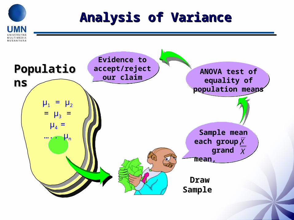
Draw Sample
PopulationsPopulations
μ1 = μ2 = μ3 = μ4 = ….. μn
Evidence to accept/reject our
claim
Sample mean each group, grand mean,
X
X
ANOVA test of equality of population
means
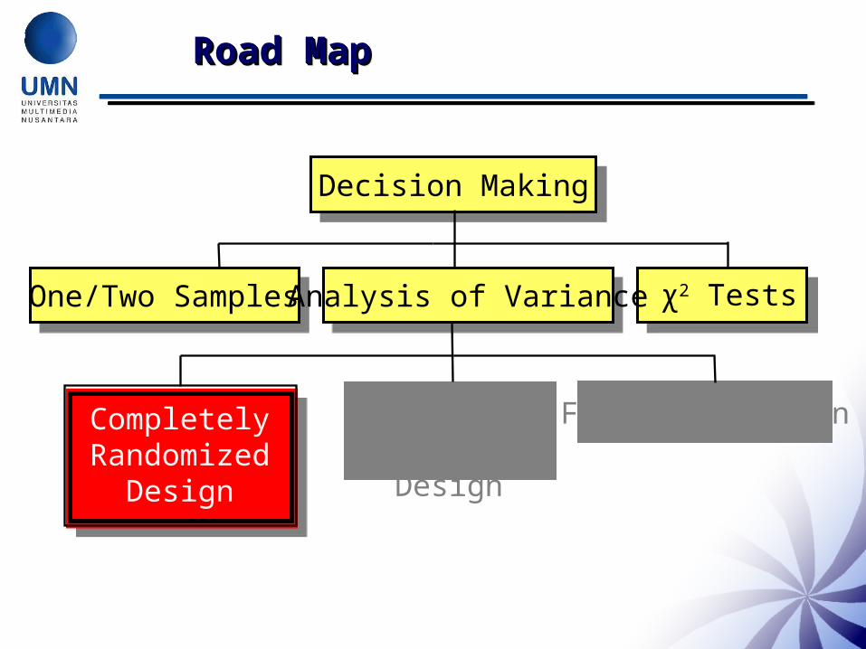
Road MapRoad MapRoad MapRoad Map
Factorial Design
Decision Making
One/Two Samples Analysis of Variance
Completely Randomized
Design
χ2 Tests
Randomized Block Design
Completely Randomized Completely Randomized DesignDesignCompletely Randomized Completely Randomized DesignDesign
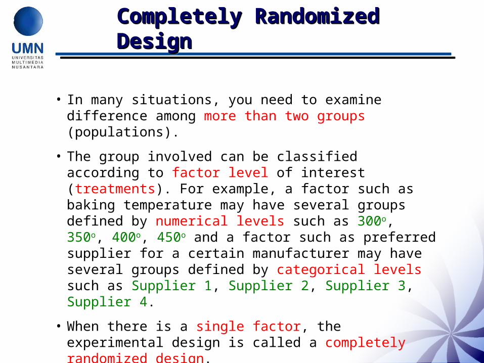
• In many situations, you need to examine difference among more than two groups (populations).
• The group involved can be classified according to factor level of interest (treatments). For example, a factor such as baking temperature may have several groups defined by numerical levels such as 300o, 350o, 400o, 450o and a factor such as preferred supplier for a certain manufacturer may have several groups defined by categorical levels such as Supplier 1, Supplier 2, Supplier 3, Supplier 4.
• When there is a single factor, the experimental design is called a completely randomized design.
One Factor Design One Factor Design ExperimentExperimentOne Factor Design One Factor Design ExperimentExperiment
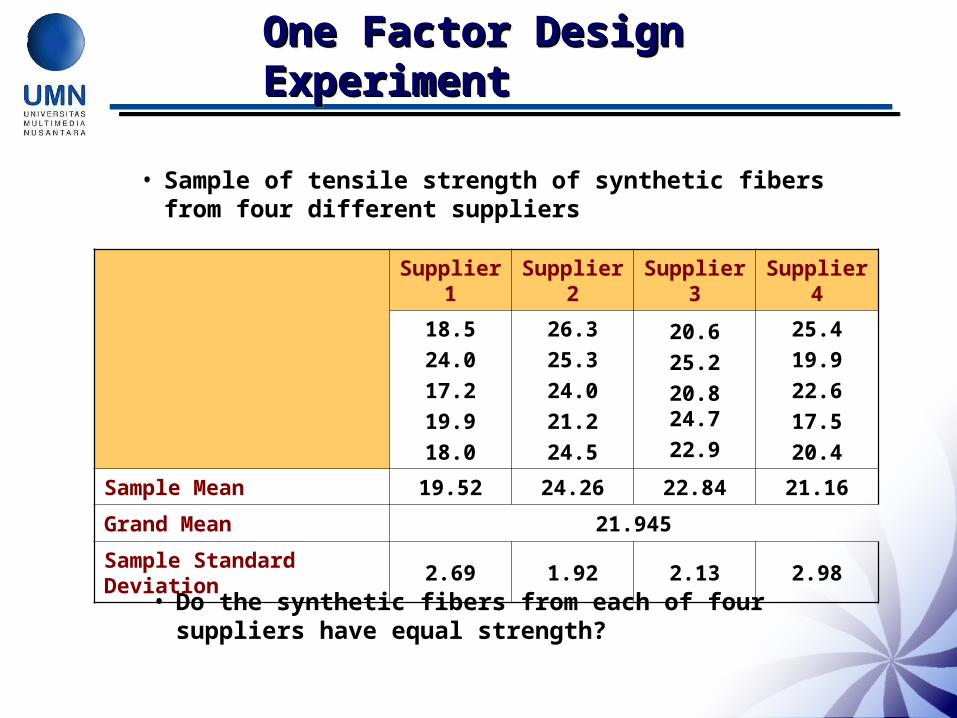
Supplier 1 Supplier 2 Supplier 3 Supplier 4
18.5
24.0
17.2
19.9
18.0
26.3
25.3
24.0
21.2
24.5
20.6
25.2
20.824.7
22.9
25.4
19.9
22.6
17.5
20.4
Sample Mean 19.52 24.26 22.84 21.16
Grand Mean 21.945
Sample Standard Deviation 2.69 1.92 2.13 2.98
• Sample of tensile strength of synthetic fibers from four different suppliers
• Do the synthetic fibers from each of four suppliers have equal strength?
One Way ANOVAOne Way ANOVAOne Way ANOVAOne Way ANOVA
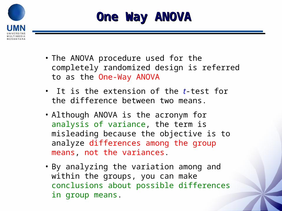
• The ANOVA procedure used for the completely randomized design is referred to as the One-Way ANOVA
• It is the extension of the t-test for the difference between two means.
• Although ANOVA is the acronym for analysis of variance, the term is misleading because the objective is to analyze differences among the group means, not the variances.
• By analyzing the variation among and within the groups, you can make conclusions about possible differences in group means.
Partitioning the Total Partitioning the Total VariationVariationPartitioning the Total Partitioning the Total VariationVariation
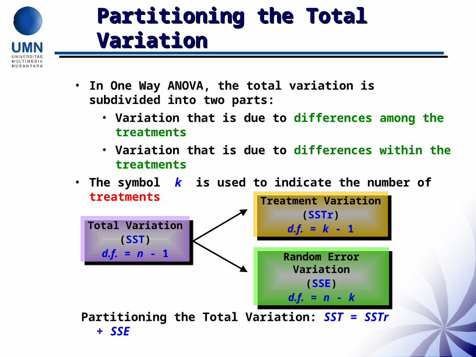
• In One Way ANOVA, the total variation is subdivided into two parts:
• Variation that is due to differences among the treatments
• Variation that is due to differences within the treatments
• The symbol k is used to indicate the number of treatments
Total Variation(SST)
d.f. = n - 1
Total Variation(SST)
d.f. = n - 1
Treatment Variation(SSTr)
d.f. = k - 1
Treatment Variation(SSTr)
d.f. = k - 1
Random Error Variation(SSE)
d.f. = n - k
Random Error Variation(SSE)
d.f. = n - k
Partitioning the Total Variation: SST = SSTr + SSE
Hypothesis to be Hypothesis to be TestedTestedHypothesis to be Hypothesis to be TestedTested
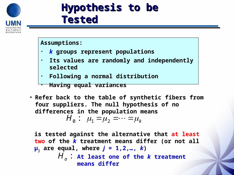
Assumptions:• k groups represent populations• Its values are randomly and independently selected• Following a normal distribution• Having equal variances
• Refer back to the table of synthetic fibers from four suppliers. The null hypothesis of no differences in the population means
kH 210 :
is tested against the alternative that at least two of the k treatment means differ (or not all μj are equal, where j = 1,2,…, k)
:aH At least one of the k treatment means differ
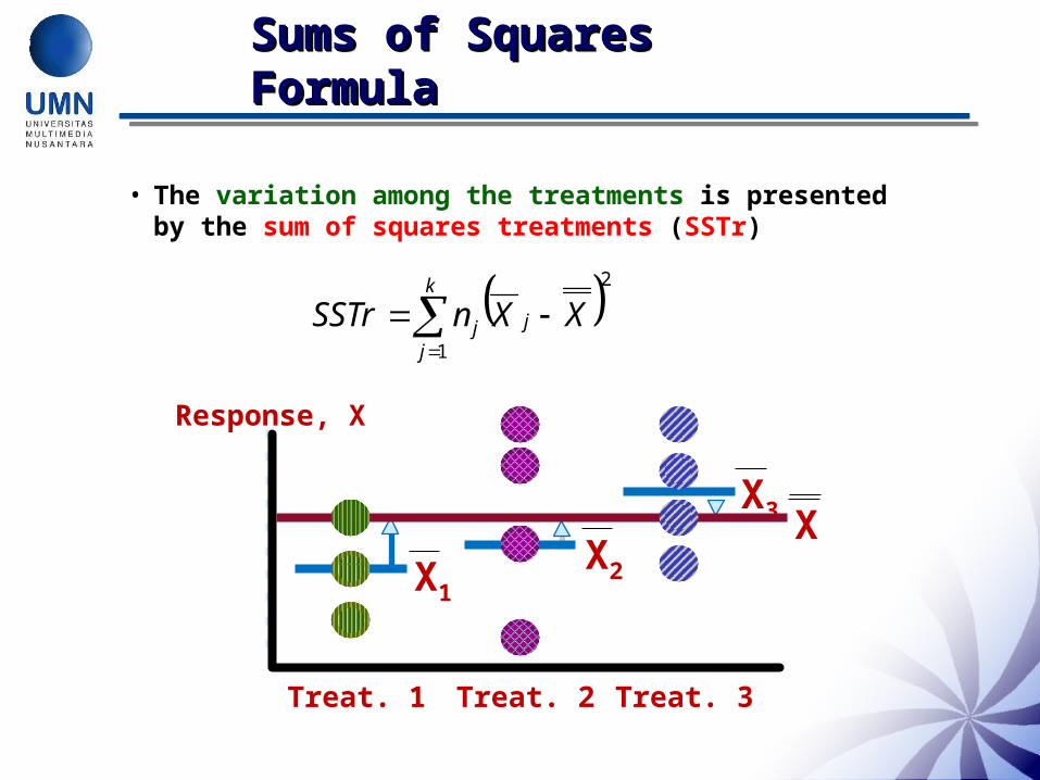
Sums of Squares Sums of Squares FormulaFormulaSums of Squares Sums of Squares FormulaFormula
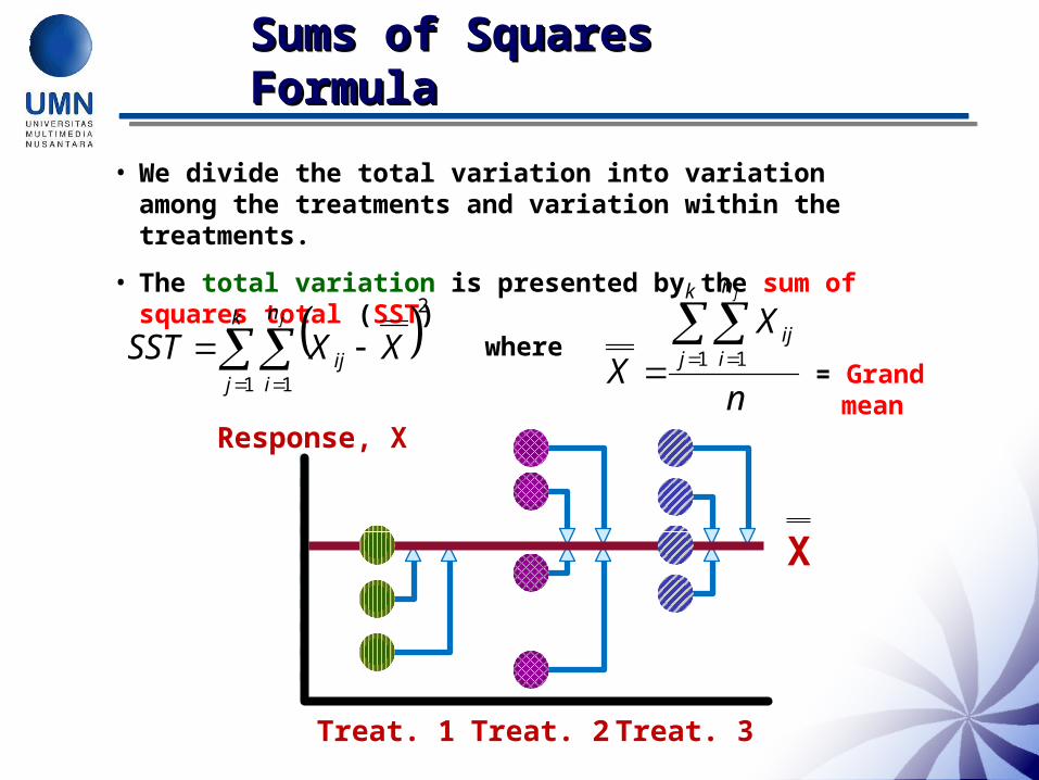
• We divide the total variation into variation among the treatments and variation within the treatments.
• The total variation is presented by the sum of squares total (SST)
2
1 1
k
j
n
iij
j
XXSST where
n
X
X
k
j
n
iij
j
1 1
= Grand mean
X
Treat. 1 Treat. 2 Treat. 3
Response, X
Sums of Squares Sums of Squares FormulaFormulaSums of Squares Sums of Squares FormulaFormula
• The variation among the treatments is presented by the sum of squares treatments (SSTr)
21
k
j
jj XXnSSTr
XX3
X2X1
Treat. 1 Treat. 2 Treat. 3
Response, X
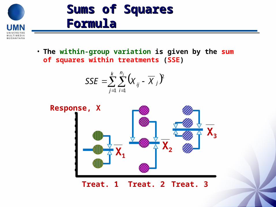
• The within-group variation is given by the sum of squares within treatments (SSE)
k
j
n
i
jij
j
XXSSE1 1
2
Sums of Squares Sums of Squares FormulaFormulaSums of Squares Sums of Squares FormulaFormula
X2X1
X3
Treat. 1 Treat. 2 Treat. 3
Response, X
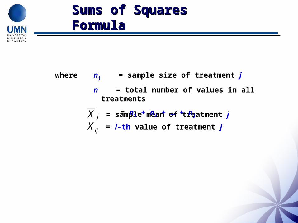
where
jX
ijX= sample mean of treatment j
= i-th value of treatment j
nj = sample size of treatment j
n = total number of values in all treatments
= n1 + n2 + … + nj
Sums of Squares Sums of Squares FormulaFormulaSums of Squares Sums of Squares FormulaFormula
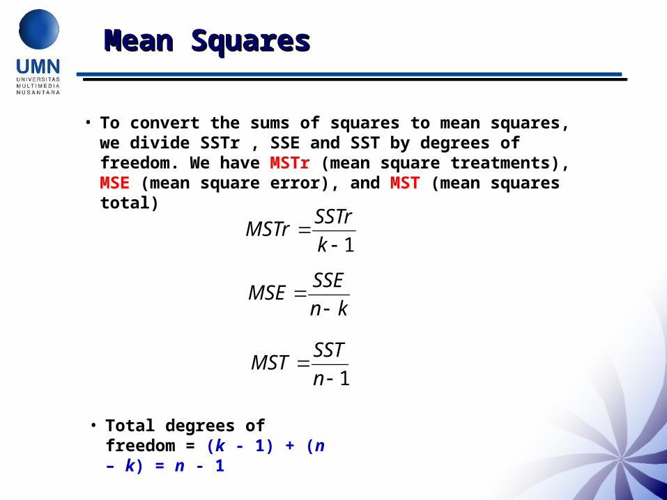
• To convert the sums of squares to mean squares, we divide SSTr , SSE and SST by degrees of freedom. We have MSTr (mean square treatments), MSE (mean square error), and MST (mean squares total)
1k
SSTrMSTr
kn
SSEMSE
Mean Mean SquaresSquaresMean Mean SquaresSquares
• Total degrees of freedom = (k - 1) + (n – k) = n - 1
1n
SSTMST
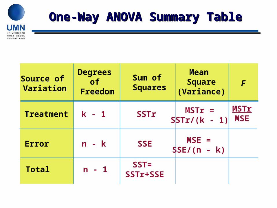
Source of Variation
Degreesof
Freedom
Sum of Squares
Mean Square
(Variance)F
Treatment k - 1 SSTr MSTr =SSTr/(k - 1)
MSTrMSE
Error n - k SSE MSE =SSE/(n - k)
Total n - 1SST=
SSTr+SSE
One-Way ANOVA Summary One-Way ANOVA Summary TableTableOne-Way ANOVA Summary One-Way ANOVA Summary TableTable
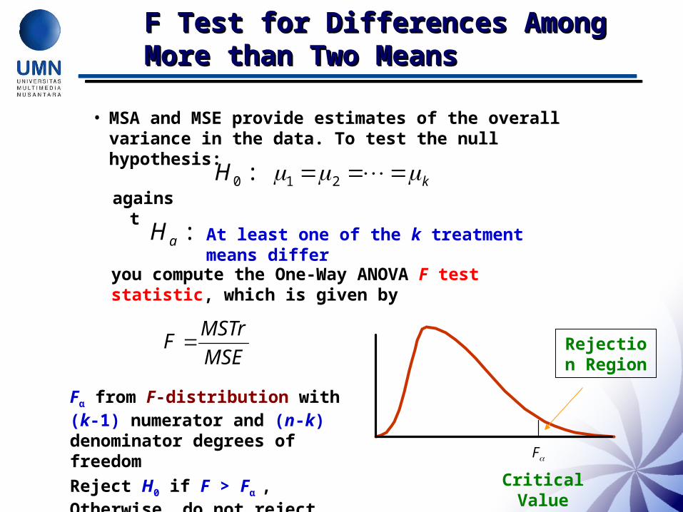
F Test for Differences Among F Test for Differences Among More than Two MeansMore than Two MeansF Test for Differences Among F Test for Differences Among More than Two MeansMore than Two Means
• MSA and MSE provide estimates of the overall variance in the data. To test the null hypothesis:
kH 210 :
:aH At least one of the k treatment means differ
against
you compute the One-Way ANOVA F test statistic, which is given by
MSE
MSTrF
F
Rejection Region
Critical Value
Fα from F-distribution with (k-1) numerator and (n-k) denominator degrees of freedom
Reject H0 if F > Fα , Otherwise, do not reject
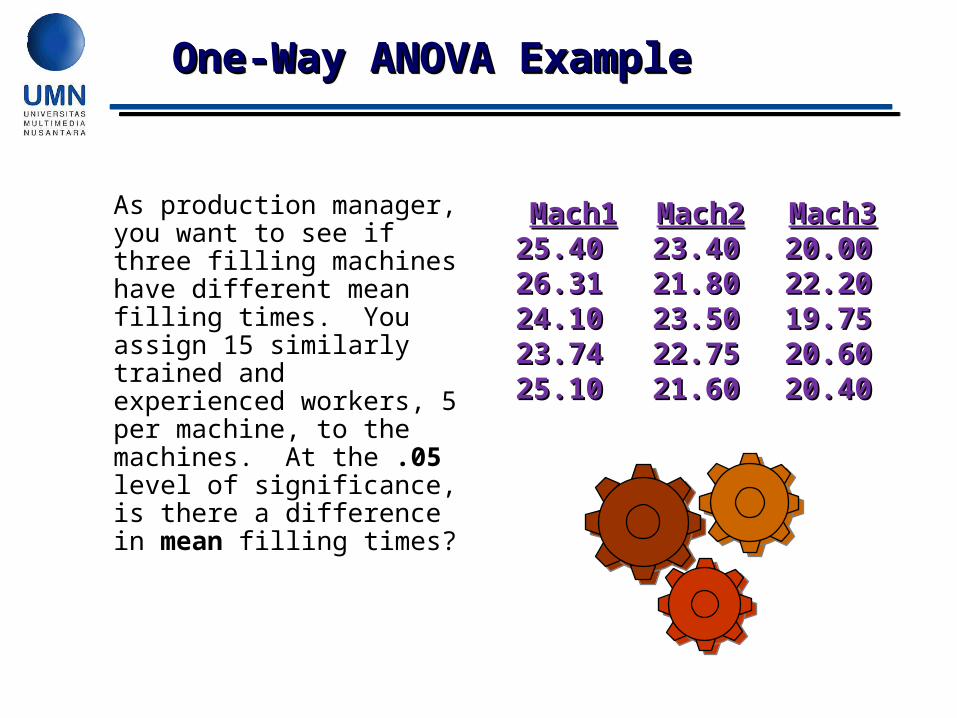
As production manager, you want to see if three filling machines have different mean filling times. You assign 15 similarly trained and experienced workers, 5 per machine, to the machines. At the .05 level of significance, is there a difference in mean filling times?
Mach1Mach1 Mach2Mach2 Mach3Mach325.4025.40 23.4023.40 20.0020.0026.3126.31 21.8021.80 22.2022.2024.1024.10 23.5023.50 19.7519.7523.7423.74 22.7522.75 20.6020.6025.1025.10 21.6021.60 20.4020.40
One-Way ANOVA One-Way ANOVA ExampleExampleOne-Way ANOVA One-Way ANOVA ExampleExample
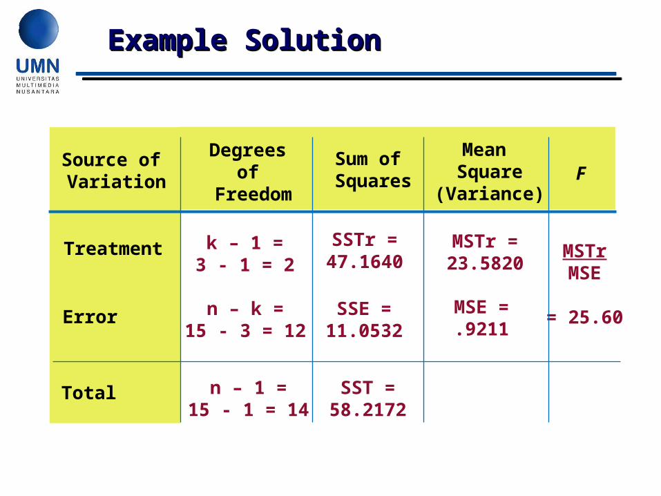
Treatment k – 1 =3 - 1 = 2
SSTr =47.1640
MSTr =23.5820
MSTrMSE
= 25.60Error n – k =15 - 3 = 12
SSE =11.0532
MSE =.9211
Total n – 1 =15 - 1 = 14
SST =58.2172
Source of Variation
Degreesof
Freedom
Sum of Squares
Mean Square
(Variance)F
Example SolutionExample SolutionExample SolutionExample Solution
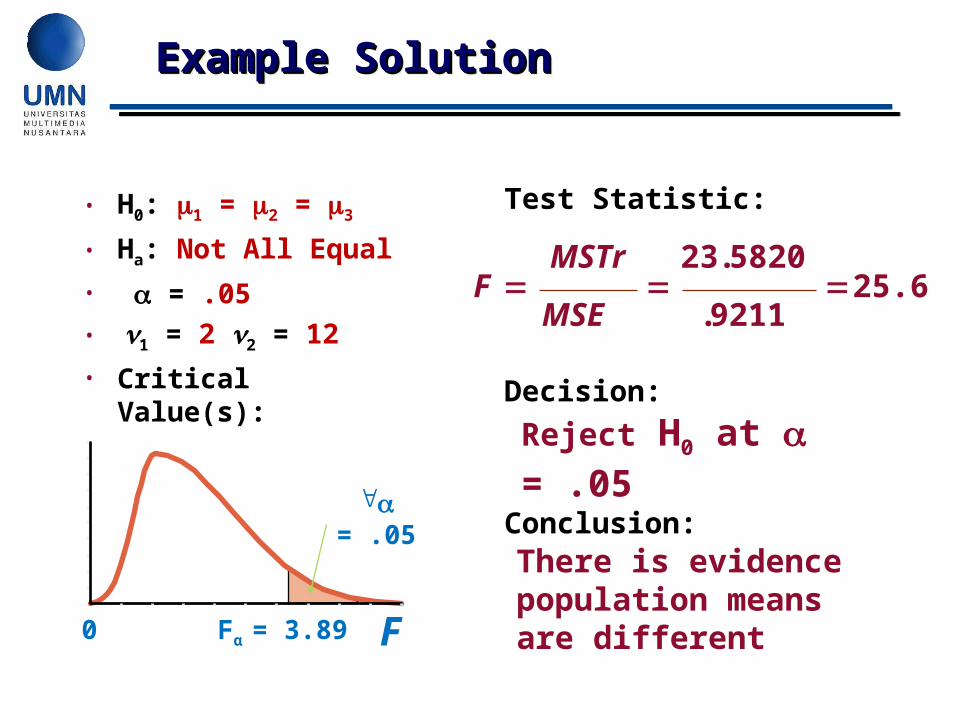
F0 Fα = 3.89
• H0: 1 = 2 = 3
• Ha: Not All Equal
• = .05• 1 = 2 2 = 12
• Critical Value(s):
Test Statistic:
Decision:
Conclusion:
Reject H0 at = .05
There is evidence population means are different
= .05
FMSTr
MSE
23 5820
921125.6
.
.
Example SolutionExample SolutionExample SolutionExample Solution

You’re a trainer for Microsoft Corp. Is there a difference in mean learning times of 12 people using 4 different training methods ( =.05)?
M1 M2 M3 M410 11 13 18
9 16 8 235 9 9 25
Use the following values.
ExerciseExerciseExerciseExercise
SSTr = 348 SSE = 80
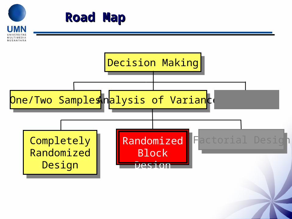
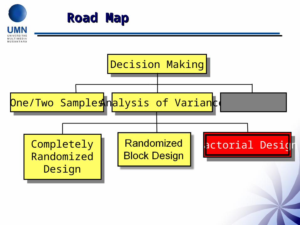
Factorial Design
Decision Making
One/Two Samples Analysis of Variance
Completely Randomized
Design
χ2 Tests
Road MapRoad MapRoad MapRoad Map
Randomized Block Design
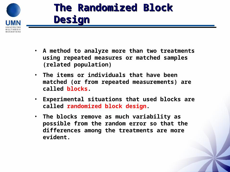
The Randomized Block The Randomized Block DesignDesignThe Randomized Block The Randomized Block DesignDesign
• A method to analyze more than two treatments using repeated measures or matched samples (related population)
• The items or individuals that have been matched (or from repeated measurements) are called blocks.
• Experimental situations that used blocks are called randomized block design.
• The blocks remove as much variability as possible from the random error so that the differences among the treatments are more evident.
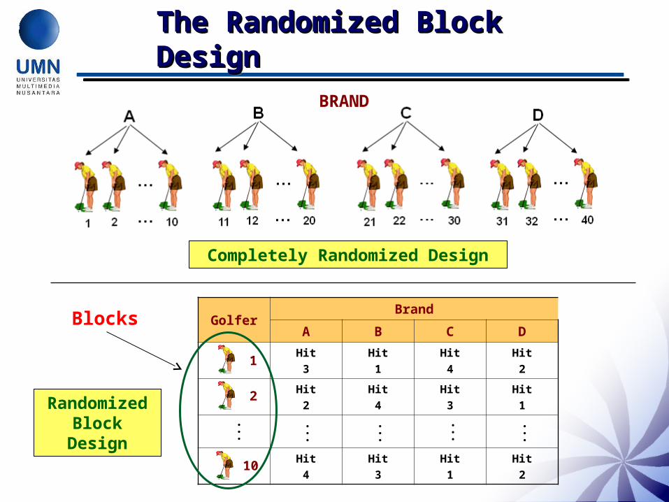
The Randomized Block The Randomized Block DesignDesignThe Randomized Block The Randomized Block DesignDesign
BRAND
GolferBrand
A B C D
Hit
3
Hit
1
Hit
4
Hit
2
Hit
2
Hit
4
Hit
3
Hit
1
Hit
4
Hit
3
Hit
1
Hit
2
1
2
10
Randomized Block Design
Completely Randomized Design
Blocks
Partitioning the Total Partitioning the Total VariationVariationPartitioning the Total Partitioning the Total VariationVariation
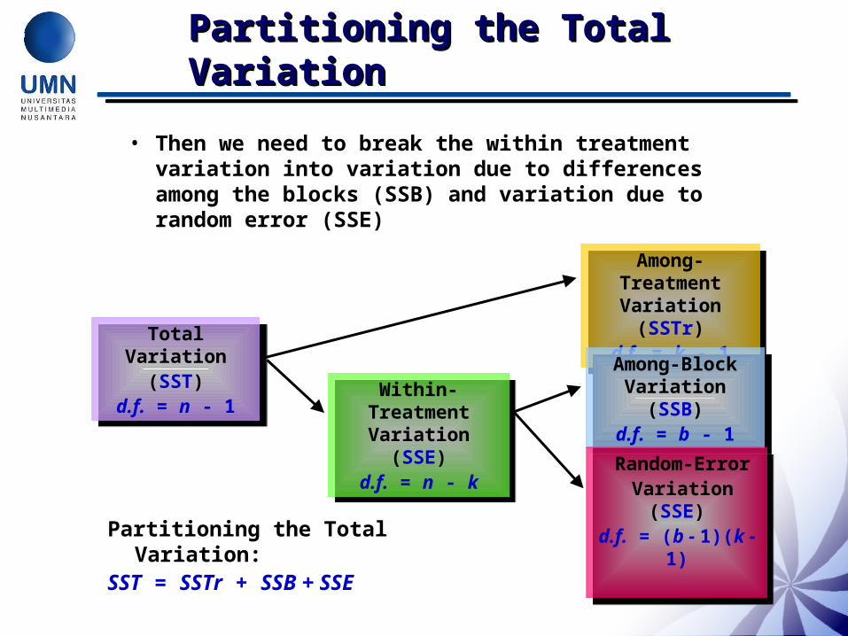
• Then we need to break the within treatment variation into variation due to differences among the blocks (SSB) and variation due to random error (SSE)
Total Variation(SST)
d.f. = n - 1
Total Variation(SST)
d.f. = n - 1
Among-Treatment Variation (SSTr)
d.f. = k - 1
Among-Treatment Variation (SSTr)
d.f. = k - 1
Within-Treatment Variation (SSE)
d.f. = n - k
Within-Treatment Variation (SSE)
d.f. = n - k
Among-Block Variation (SSB)
d.f. = b - 1
Among-Block Variation (SSB)
d.f. = b - 1
Random-Error Variation (SSE)d.f. = (b - 1)(k - 1)
Random-Error Variation (SSE)d.f. = (b - 1)(k - 1)
Partitioning the Total Variation:SST = SSTr + SSB + SSE
Sums of Squares Sums of Squares FormulaFormulaSums of Squares Sums of Squares FormulaFormula
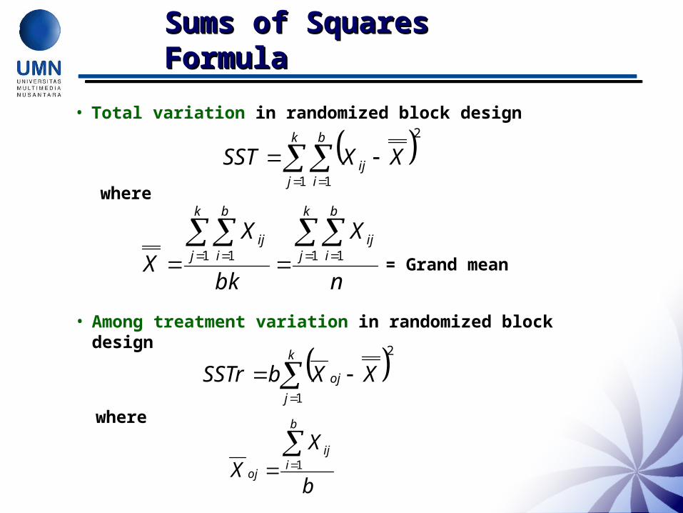
• Total variation in randomized block design
21 1
k
j
b
iij XXSST
where
n
X
bk
X
X
k
j
b
iij
k
j
b
iij
1 11 1= Grand mean
• Among treatment variation in randomized block design
21
k
j
oj XXbSSTr
where
b
XX
b
iij
oj
1

• Among block variation in randomized block design
21
b
i
io XXkSSB
• Random error in randomized block design
k
j
b
i
ojioij XXXXSSE1 1
2
Sums of Squares Sums of Squares FormulaFormulaSums of Squares Sums of Squares FormulaFormula
where
k
X
X
k
jij
io
1
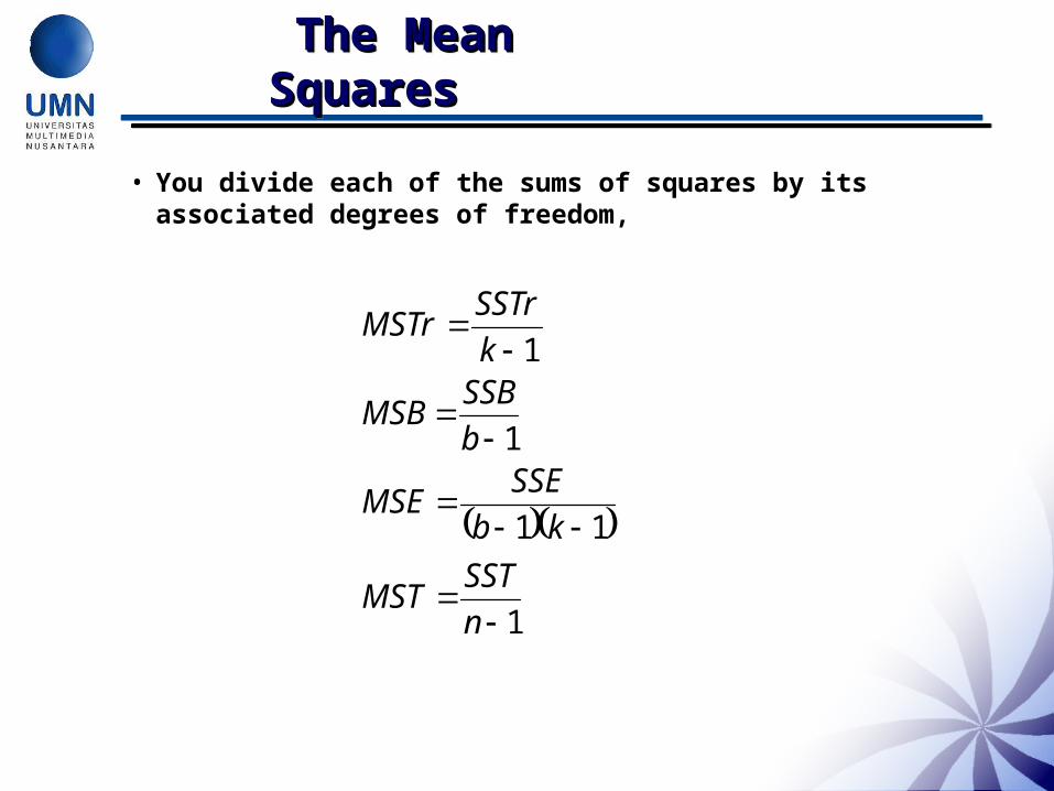
• You divide each of the sums of squares by its associated degrees of freedom,
The Mean The Mean SquaresSquares The Mean The Mean SquaresSquares
1
11
1
1
n
SSTMST
kb
SSEMSE
b
SSBMSB
k
SSTrMSTr

• The null hypothesis
Randomized Block Randomized Block FF TestsTestsRandomized Block Randomized Block FF TestsTests
is tested against
F test statistic
You reject the null hypothesis at the α level if
Fα from F distribution with (k-1) numerator and (k-1) (b-1) denominator degrees of freedom
kH 210 :
MSE
MSTrFT
FFT
:aH At least one of the k treatment means differ

• The null hypothesis
FF Tests for Block Tests for Block EffectsEffectsFF Tests for Block Tests for Block EffectsEffects
is tested against
F test statistic
You reject the null hypothesis at the α level if
Fα from F distribution with (b-1) numerator and (k-1) (b-1) denominator degrees of freedom
bH 210 :
MSE
MSBFB
FFB
:aH At least one of the b block means differ
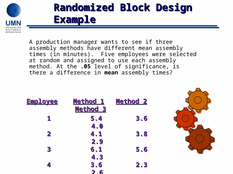
A production manager wants to see if three assembly methods have different mean assembly times (in minutes). Five employees were selected at random and assigned to use each assembly method. At the .05 level of significance, is there a difference in mean assembly times?
EmployeeEmployee Method 1Method 1 Method 2Method 2 Method 3Method 3
11 5.45.4 3.63.64.04.0
22 4.14.1 3.83.82.92.9
33 6.16.1 5.65.64.34.3
44 3.63.6 2.32.32.62.6
55 5.35.3 4.74.73.43.4
Randomized Block Design Randomized Block Design ExampleExampleRandomized Block Design Randomized Block Design ExampleExample
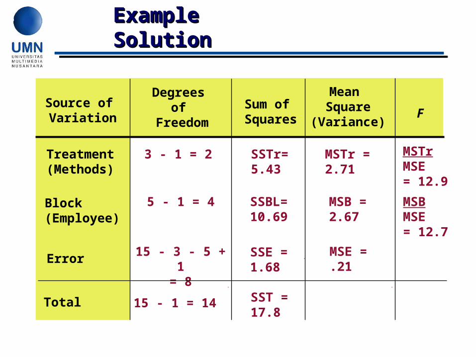
Treatment(Methods)
3 - 1 = 2 SSTr=5.43
MSTr = 2.71
MSTrMSE= 12.9
Error15 - 3 - 5 + 1
= 8SSE =1.68
MSE =.21
Total 15 - 1 = 14 SST =17.8
Source of Variation
Degreesof
Freedom
Sum of Squares
Mean Square
(Variance)F
Block(Employee)
5 - 1 = 4 SSBL=10.69
MSB =2.67
MSBMSE= 12.7
Example Example SolutionSolutionExample Example SolutionSolution
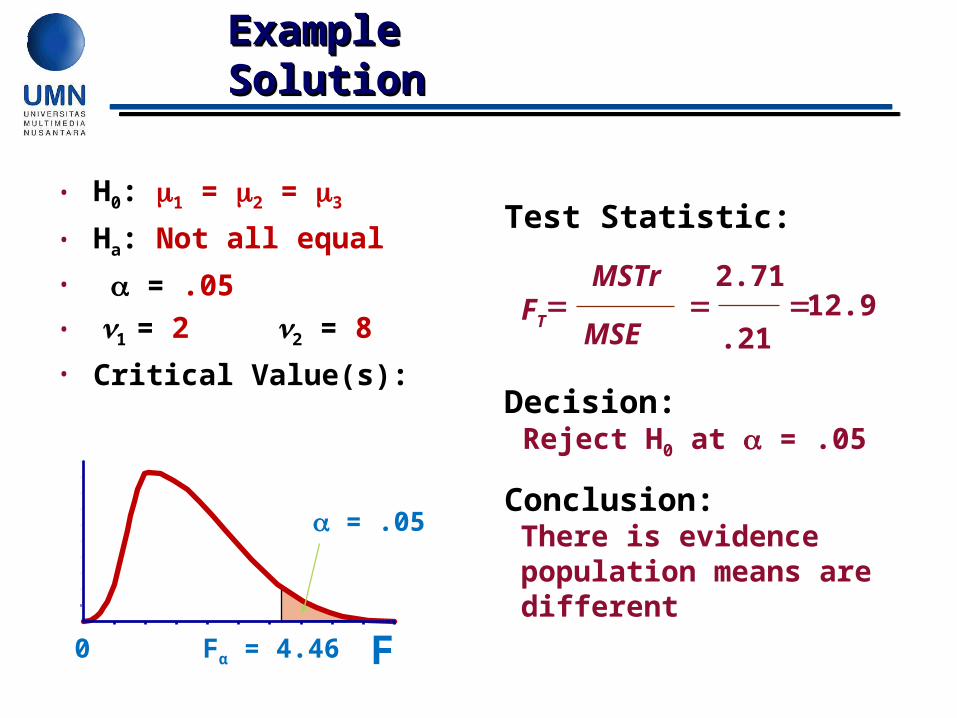
F0 Fα = 4.46
• H0: 1 = 2 = 3
• Ha: Not all equal
• = .05• 1 = 2 2 = 8
• Critical Value(s):
Test Statistic:
Decision:
Conclusion:
Reject H0 at = .05
There is evidence population means are different
= .05
FT
MSTr
MSE
2.71
.2112.9
Example Example SolutionSolutionExample Example SolutionSolution
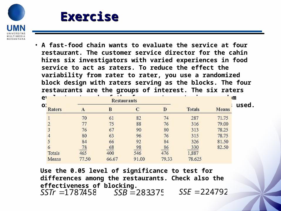
• A fast-food chain wants to evaluate the service at four restaurant. The customer service director for the cahin hires six investigators with varied experiences in food service to act as raters. To reduce the effect the variability from rater to rater, you use a randomized block design with raters serving as the blocks. The four restaurants are the groups of interest. The six raters evaluate at each of the four restaurants in a random order. A rating scale from 0 (low) to 100 (high) is used.
ExerciseExerciseExerciseExercise
Use the 0.05 level of significance to test for differences among the restaurants. Check also the effectiveness of blocking.
458.1787SSTr 375.283SSB 792224.SSE
Road MapRoad MapRoad MapRoad Map
Decision Making
One/Two Samples Analysis of Variance
Completely Randomized
Design
χ2 Tests
Factorial Design
The Factorial The Factorial Design Design The Factorial The Factorial Design Design
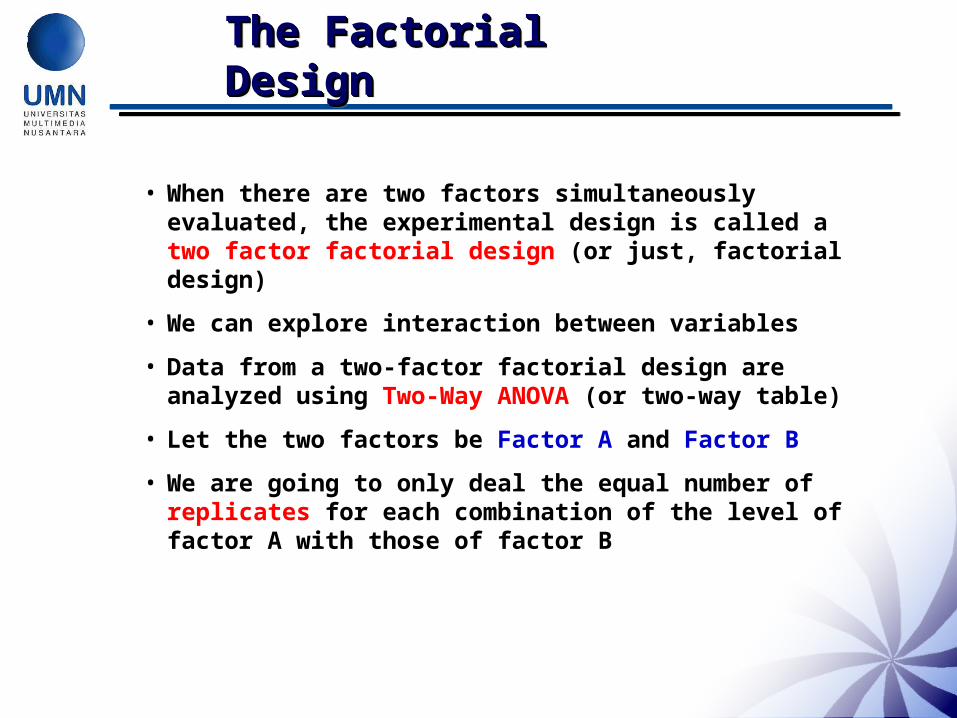
• When there are two factors simultaneously evaluated, the experimental design is called a two factor factorial design (or just, factorial design)
• We can explore interaction between variables
• Data from a two-factor factorial design are analyzed using Two-Way ANOVA (or two-way table)
• Let the two factors be Factor A and Factor B
• We are going to only deal the equal number of replicates for each combination of the level of factor A with those of factor B
Example of Two Factors Example of Two Factors Design Design Example of Two Factors Example of Two Factors Design Design
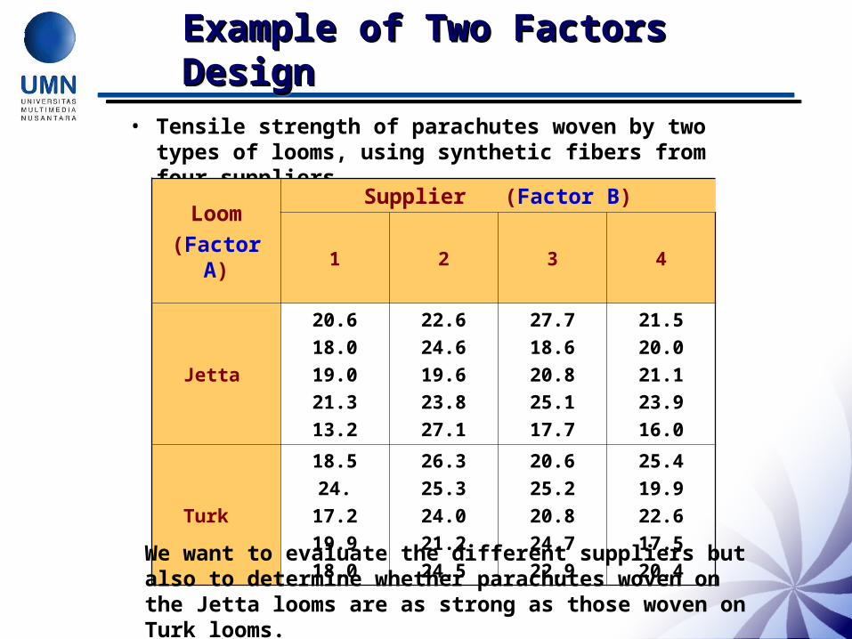
• Tensile strength of parachutes woven by two types of looms, using synthetic fibers from four suppliers
Loom
(Factor A)
Supplier (Factor B)
1 2 3 4
Jetta
20.6
18.0
19.0
21.3
13.2
22.6
24.6
19.6
23.8
27.1
27.7
18.6
20.8
25.1
17.7
21.5
20.0
21.1
23.9
16.0
Turk
18.5
24.
17.2
19.9
18.0
26.3
25.3
24.0
21.2
24.5
20.6
25.2
20.8
24.7
22.9
25.4
19.9
22.6
17.5
20.4We want to evaluate the different suppliers but also to determine whether parachutes woven on the Jetta looms are as strong as those woven on Turk looms.
Two Way ANOVA Two Way ANOVA Procedure Procedure Two Way ANOVA Two Way ANOVA Procedure Procedure
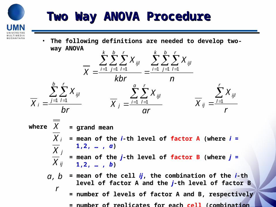
• The following definitions are needed to develop two-way ANOVA
n
X
kbr
X
X
k
i
b
j
r
lijl
k
i
b
j
r
lijl
1 1 11 1 1
br
X
X
b
j
r
lijl
i
1 1
ar
XX
a
i
r
lijl
j
1 1
r
XX
r
lijl
ij
1
where = grand mean
= mean of the i-th level of factor A (where i = 1,2, … , a)
= mean of the j-th level of factor B (where j = 1,2, … , b)
= mean of the cell ij, the combination of the i-th level of factor A and the j-th level of factor B
= number of levels of factor A and B, respectively
= number of replicates for each cell (combination of a particular level of factor A and that of factor B)
iXX
jX
ijX
b,a
r

Main and Interaction Main and Interaction Effects Effects Main and Interaction Main and Interaction Effects Effects
No A effect; B main effect
1 2 3
Me
an
re
sp
on
se
Level of factor A
Level 1, factor B
Level 2, factor B
1 2 3
Me
an
re
sp
on
se
Level of factor A
Level 1, factor BLevel 2, factor B
A main effect; insignificant B effect
A and B main effects, no interaction
1 2 3
Me
an
re
sp
on
se
Level of factor A
Level 1, factor B
Level 2, factor B
A and B interact
1 2 3
Me
an
re
sp
on
se
Level of factor A
Level 1, factor B
Level 2, factor B
Partitioning the Total Partitioning the Total Variation Variation Partitioning the Total Partitioning the Total Variation Variation
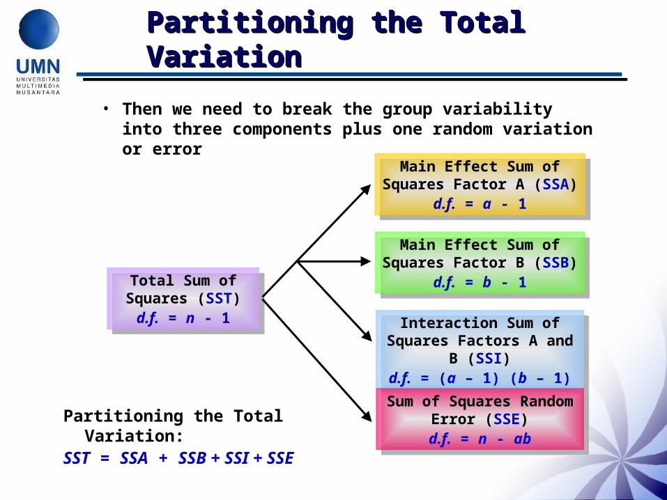
• Then we need to break the group variability into three components plus one random variation or error
Total Sum of Squares (SST)
d.f. = n - 1
Total Sum of Squares (SST)
d.f. = n - 1Interaction Sum of Squares
Factors A and B (SSI)d.f. = (a – 1) (b – 1)
Interaction Sum of Squares Factors A and B (SSI)
d.f. = (a – 1) (b – 1)
Sum of Squares Random Error (SSE)d.f. = n - ab
Sum of Squares Random Error (SSE)d.f. = n - ab
Main Effect Sum of Squares Factor A (SSA)
d.f. = a - 1
Main Effect Sum of Squares Factor A (SSA)
d.f. = a - 1
Main Effect Sum of Squares Factor B (SSB)
d.f. = b - 1
Main Effect Sum of Squares Factor B (SSB)
d.f. = b - 1
Partitioning the Total Variation:SST = SSA + SSB + SSI + SSE
Sum of Squares Sum of Squares FormulaFormulaSum of Squares Sum of Squares FormulaFormula
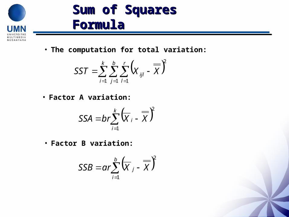
• The computation for total variation:
21 1 1
k
i
b
j
r
lijl XXSST
• Factor A variation:
21
k
i
i XXbrSSA
• Factor B variation:
21
b
i
j XXarSSB
Sum of Squares Sum of Squares FormulaFormulaSum of Squares Sum of Squares FormulaFormula
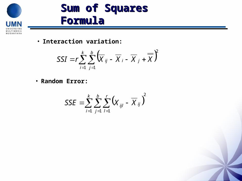
• Interaction variation:
21 1
k
i
b
j
jiij XXXXrSSI
• Random Error:
2
1 1 1
k
i
b
j
r
l
ijijl XXSSE
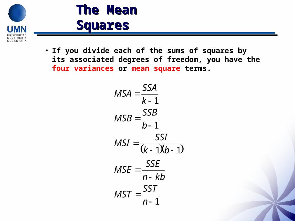
The Mean The Mean SquaresSquaresThe Mean The Mean SquaresSquares
• If you divide each of the sums of squares by its associated degrees of freedom, you have the four variances or mean square terms.
1
11
1
1
n
SSTMST
kbn
SSEMSE
bk
SSIMSI
b
SSBMSB
k
SSAMSA
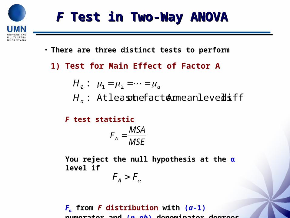
• There are three distinct tests to perform
FF Test in Two-Way Test in Two-Way ANOVAANOVAFF Test in Two-Way Test in Two-Way ANOVAANOVA
1) Test for Main Effect of Factor A
F test statistic
You reject the null hypothesis at the α level if
Fα from F distribution with (a-1) numerator and (n-ab) denominator degrees of freedom
differ levelsmean A factor oneleast At :
: 210
a
a
H
H
MSE
MSAFA
FFA
FF Test in Two-Way Test in Two-Way ANOVAANOVAFF Test in Two-Way Test in Two-Way ANOVAANOVA
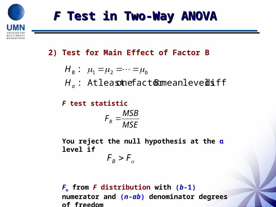
2) Test for Main Effect of Factor B
F test statistic
You reject the null hypothesis at the α level if
Fα from F distribution with (b-1) numerator and (n-ab) denominator degrees of freedom
differ levelsmean Bfactor oneleast At :
: 210
a
b
H
H
MSE
MSBFB
FFB
FF Test in Two-Way Test in Two-Way ANOVAANOVAFF Test in Two-Way Test in Two-Way ANOVAANOVA
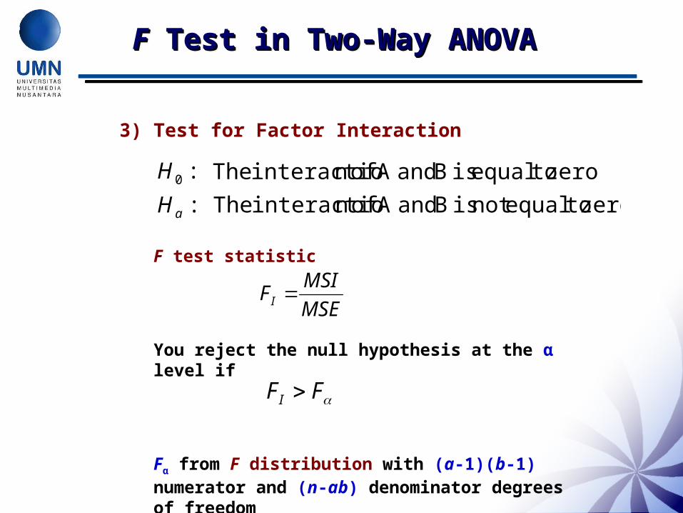
3) Test for Factor Interaction
F test statistic
You reject the null hypothesis at the α level if
Fα from F distribution with (a-1)(b-1) numerator and (n-ab) denominator degrees of freedom
zero toequalnot is B andA ofn interactio The:
zero toequal is B andA ofn interactio The:0
aH
H
MSE
MSIFI
FFI
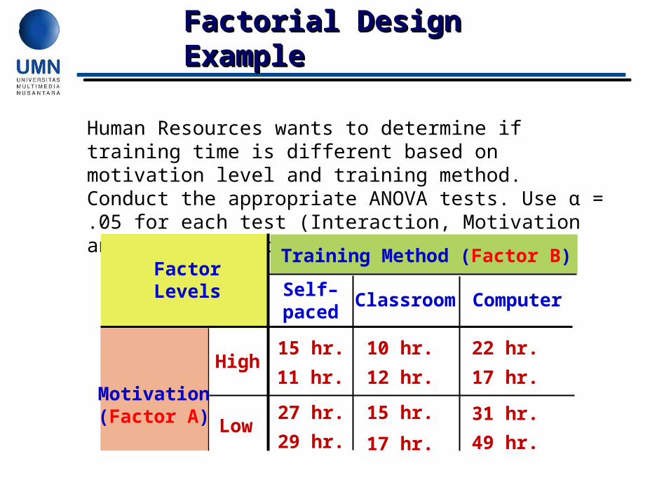
Human Resources wants to determine if training time is different based on motivation level and training method. Conduct the appropriate ANOVA tests. Use α = .05 for each test (Interaction, Motivation and Training Method).
Training Method (Factor B)FactorLevels Self–
pacedClassroom Computer
15 hr. 10 hr. 22 hr.
Motivation(Factor A)
High11 hr. 12 hr. 17 hr.
27 hr. 15 hr. 31 hr.Low
29 hr. 17 hr. 49 hr.
Factorial Design Factorial Design ExampleExampleFactorial Design Factorial Design ExampleExample
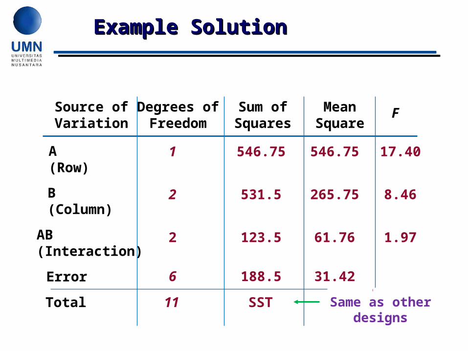
Source ofVariation
Degrees ofFreedom
Sum ofSquares
MeanSquare
F
A(Row)
1 546.75 546.75
B(Column)
2 531.5 265.75
AB(Interaction)
2 123.5 61.76
Error 6 188.5 31.42
Total 11 SST Same as other designs
17.40
8.46
1.97
Example SolutionExample SolutionExample SolutionExample Solution
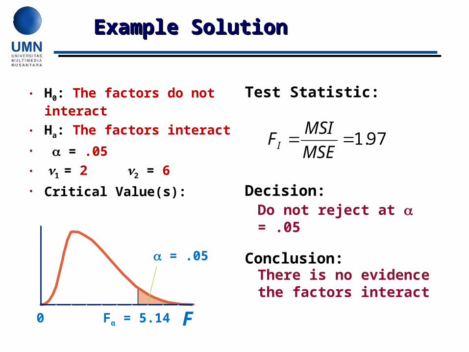
• H0: The factors do not interact
• Ha: The factors interact
• = .05• 1 = 2 2 = 6
• Critical Value(s):
Test Statistic:
Decision:
Conclusion:
F0 Fα = 5.14
= .05
Do not reject at = .05
There is no evidence the factors interact
Example SolutionExample SolutionExample SolutionExample Solution
97.1MSE
MSIFI
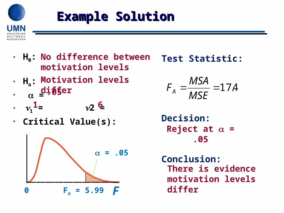
• H0:
• Ha:
• =• 1 = 2 =
• Critical Value(s):
Test Statistic:
Decision:
Conclusion:
F0 Fα = 5.99
= .05
No difference between motivation levels
Motivation levels differ
.05
1 6
Reject at = .05
There is evidence motivation levels differ
Example SolutionExample SolutionExample SolutionExample Solution
4.17MSE
MSAFA
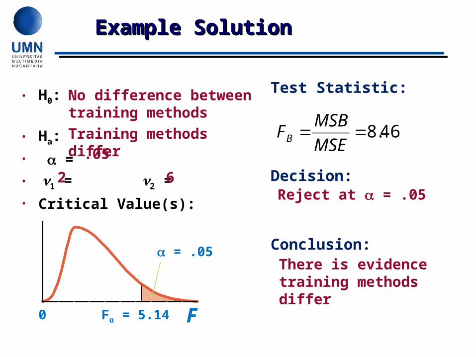
• H0:
• Ha:
• =• 1 = 2 =
• Critical Value(s):
Test Statistic:
Decision:
Conclusion:
F0 Fα = 5.14
= .05
No difference between training methods
Training methods differ.05
2 6Reject at = .05
There is evidence training methods differ
Example SolutionExample SolutionExample SolutionExample Solution
46.8MSE
MSBFB
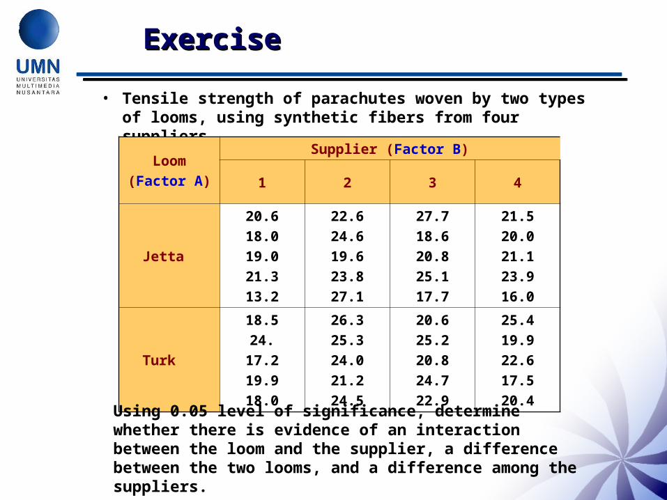
ExerciseExerciseExerciseExercise
• Tensile strength of parachutes woven by two types of looms, using synthetic fibers from four suppliers
Loom
(Factor A)
Supplier (Factor B)
1 2 3 4
Jetta
20.6
18.0
19.0
21.3
13.2
22.6
24.6
19.6
23.8
27.1
27.7
18.6
20.8
25.1
17.7
21.5
20.0
21.1
23.9
16.0
Turk
18.5
24.
17.2
19.9
18.0
26.3
25.3
24.0
21.2
24.5
20.6
25.2
20.8
24.7
22.9
25.4
19.9
22.6
17.5
20.4Using 0.05 level of significance, determine whether there is evidence of an interaction between the loom and the supplier, a difference between the two looms, and a difference among the suppliers.

ExerciseExerciseExerciseExercise
The sums of squares are already given,
972362
1
.XXbrSSAa
i
i
34881342
1
.XXarSSBb
i
j
2867.02
1 1
a
i
b
j
jiij XXXXrSSI
59202752
1 1 1
.XXSSEa
i
b
j
r
k
ijijk

Related Documents


