Top Incomes in Sweden over the Twentieth Century

Top Incomes in Sweden over the Twentieth Century1

Jesper Roine and Daniel Waldenström

7.1 INTRODUCTION

The evolution of income inequality across different economic systems has

received enormous attention. A key issue in the literature has been the

possible trade-offs between egalitarian ambitions and incentive effects. It is

not surprising therefore, that Sweden, thanks to its tradition as an

egalitarian society, has attracted disproportionate interest from inequality

scholars. However, two important aspects have largely been overlooked.

First, the lack of available micro data has led to most studies not going

further back than to 1968.2 The lack of homogenous, long-run series means

that we can not really put the developments over the past decades in

historical perspective. We do not know, for example, to what extent the

1 This chapter is an extended version of �“The Evolution of Top Incomes in an Egalitarian Society: Sweden, 1903�–2004�” published in Journal of Public Economics, 9(1-2): 366-387. In particular, the extensive appendices published here contains detailed information about sources, the Swedish income data, as well as alternatives for constructing reference totals in the Swedish case. 2 See Lindbeck (1997) for an overview of the Swedish welfare state; Atkinson et al. (1995), and Gottschalk and Smeeding (1997) for Swedish income distribution in international perspective; and, e.g. Björklund and Freeman (2006) for a recent overview of income equalization in Sweden. Examples of studies of income distribution before 1968 include Björklund and Palme (2000) who study the Swedish income distribution on decile level for four years between 1951 and 1973; Spånt�’s (1979) study of Census data for the period 1920�–1976, Lydall�’s (1968) for the period 1920�–1960; Gustafsson and Johansson (2003) who study tax returns for five separate years during the period 1925�–1958 (restricted to people living in the City of Gothenburg); Söderberg (1991) who studies salaries in various sectors between 1870 and 1950; Lindstrand (1949) studies the period 1935�–1947 and Quensel (1944) the period 1930�–1941, both using tax return data, etc. Bentzel�’s (1953) study of the period 1930�–1948 is closest to ours in methodology.

2

equal distribution of income in Sweden is mainly the outcome of the growth

of the welfare state, or if Sweden perhaps has a history of being an

egalitarian society. Second, the focus on welfare issues has resulted in most

studies concentrating on general measures of the distribution, such as the

Gini coefficient, or on the lower parts of it, but no attention has been paid

to details of top incomes. This is potentially problematic as detailed

knowledge about the top of the distribution may be crucial for distinguishing

between different explanations of what drives inequality (or the lack of it).

For example, to differentiate between theories which, on the one hand,

focus on changes in the relative wages of skilled and unskilled workers and,

on the other hand, theories that stress the importance of savings and capital

formation, we must have details about top incomes.

This chapter addresses these two shortcomings by providing new

homogenous series on top income shares in Sweden, starting at the time of

the introduction of the modern tax system in 1902 and until today. We also

propose ways of explaining these developments. In 1902 Sweden was largely

agrarian, had not yet extended the franchise to all male citizens, and was

still half a century away from the expansion of the Welfare State. Our

series, hence, allow us to study changes in income concentration over a

period during which Swedish society has undergone major structural change

and also allow us to add the historical perspective on income inequality in

Sweden which previously has not been available. The fact that we can

decompose income shares with respect to the source of income, as well as

study smaller fractiles within the top of the distribution (from the top 10

percent to the top 0.01 percent), enables us to discriminate between the

3

possible economic mechanisms that could explain our findings. As changes in

wealth concentration and in particular wealth distribution by income class

are important for understanding changes in top income shares we provide

new series for these developments over the twentieth century.

This study can, of course, also be seen as a contribution to the recent

work on long-run income inequality in which series of income concentration

have been constructed using a common methodology.3 These studies have

given numerous new insights to changes in income concentration and in

particular noted common developments for Anglo-Saxon countries, on the

one hand, and continental European countries, on the other. As our study is

concerned with one of the extremes of what Esping-Andersen (1990)

denotes �“the different worlds of welfare capitalism�” namely the social

democratic welfare state, it is particularly interesting to compare our

findings to the previous work.4 It turns out that Sweden is indeed different

from both the Anglo-Saxon as well as the Continental European group of

countries, although not entirely in ways which may have been expected.

3 Following the first studies by Piketty (2001a, 2003) on France, Piketty and Saez (2003) on the US, and Atkinson on the U.K. (2004), other recent studies include Australia (Atkinson and Leigh, 2007), Canada (Saez and Veall, 2005), Germany (Dell, 2005), Ireland (Nolan, 2005), Japan (Moriguchi and Saez, 2006), the Netherlands (Atkinson and Salverda, 2005), New Zealand (Atkinson and Leigh, 2007), Spain (Alvaredo and Saez, Chapter 10 in this volume) and Switzerland (Dell, Piketty and Saez, 2007). Atkinson and Piketty (2007) collect much of this work. Lindert (2000) and Morrisson (2000) provide surveys of previous studies on long run inequality developments. 4 In his distinction between �“The Three Worlds of Welfare Capitalism�”, Esping-Andersen (1990) identifies three different types of welfare states; �“liberal welfare states�” (e.g., the U.S. and the U.K.), the �“corporatist-conservative welfare states�” (e.g., France, Germany, Italy) and the �“social democratic welfare states�”. A similar distinction is often made between an Anglo-Saxon, a Continental European, and a Scandinavian group of countries; see, e.g., Lindbeck (2006).

4

A number of broad facts stand out from our series. Over the first

eighty years of the twentieth century top income shares in Sweden

decreased. Most of this decrease happened during the first half of the

century, that is, before the expansion of the Welfare State, and most of it

was due to large falls in the income share of the top percentile (P99�–100).

By contrast, the income share going to the lower half of the top decile (P90�–

P95), which consists mainly of wages, has been remarkably stable over the

entire period. Between 1903 and 2006 this share has fluctuated between 9

and 11 percent, while the top percentile has changed by a factor of four.

This suggests that decomposing the top decile into smaller fractions is

crucial for understanding the development. In terms of composition, most of

the early decrease seems to have been driven by falls in capital income, but

after around the mid-1930s wage compression also becomes important in

explaining the decreasing top shares. The drops in capital shares fit well

with sharp decreases in top wealth shares during the first half of the

century, in particular in the early 1930s, but notably not during the Second

World War, as was the case in many other countries. Between 1950 and

1980 the continued decrease in inequality was quite steady but smaller

relative to the first half of the century. Over the past two decades the

general picture turns out to depend crucially on how income from capital

gains is treated.5 If we include capital gains, Swedish income inequality has

increased quite substantially; when excluding them, top income shares have

increased much less. This indicates that while labor incomes have not 5 It is important to note that throughout the chapter, whenever we refer to capital gains income, this means realized capital gains, which is what the tax data allow us to measure. In section 7.3 below we discuss possible implications of this distinction in more detail.

5

diverged dramatically over the past decades, the gains from exceptionally

large increases in asset prices (mainly increases in share prices) have been

very unevenly distributed.6 This, in turn, suggests that the Swedish case

over the past decades is different from both the Anglo-Saxon case as well as

from the continental European case previously identified in the literature.7

The remainder of the chapter is organized as follows: In Section 7.2

we discuss the data and methodology used, in Section 7.3 we present our

main findings under four sub-headings; first we account for the evolution of

top income shares in terms of gross income from all sources (separating

series including and excluding capital gains), second we study the

composition of these shares by source, third we analyze the effect of

potential tax avoidance and evasion on our series, and fourth we study

separate top income series when excluding taxable transfers giving us an

income concept closer to market income.8 Thereafter we attempt to

account for our results in Section 7.4 by studying changes in factor shares,

the wealth distribution, tax progressivity, and changes in asset prices. In

Section 7.5 we highlight differences and similarities in our results for

Sweden with the findings in a number of other countries for which

comparable data exist. Section 7.6 concludes. A number of appendices

6 Our data suggest that these capital gains have accrued to those who also have the highest wages, hence magnifying inequalities in the income distribution. 7 See, e.g., Saez (2004) and Piketty and Saez (2006) for cross-country comparisons. 8 For most other countries this distinction is not very important when studying top incomes, but in the Swedish context (taxable) social transfers are sufficiently large to have an effect on the top income shares, even if they do not make up any large part of top incomes, as including them affects the reference total for income (see, for example, Björklund and Freeman (2006) on the importance of transfers for income distribution in Sweden).

6

contain detailed information about data and various adjustments as well as

sensitivity analysis of our main series.

7.2 METHODOLOGY AND DATA

In recent years, a methodology for studying income concentration using long

time series of tax return data has been established following Piketty

(2001a), who in turn builds on the seminal work by Kuznets (1953). The

basic idea is to construct shares of total personal income received by

different fractiles of the entire (tax) population, had everyone been

required to file a tax return. Since historically only top income earners were

taxed they are the only ones directly observed over the entire period. This

in turn means that the reference totals for population and income, which

are aimed at also including individuals who did not file a tax return and

their incomes, must be constructed using aggregate sources from the

population statistics and national accounts. Top income shares are then

computed by dividing the number of tax units in the top, and their incomes,

by the reference tax population and reference total income.9 Assuming that

top incomes are approximately Pareto distributed, standard inter- and

9 There are, of course, a number of potential problems with using tax statistics data; it is collected as part of an administrative routine in which individuals have incentives to underreport income, it tells us nothing per se about the welfare of individuals, etc. Nevertheless, as long as we think that tax statistics, at least for the top income earners, approximate actual incomes, and as long as the problems with the statistics have not changed systematically over time, they are a useful source. Importantly, it is also the only available source for much of the twentieth century. Our general view in the case of Sweden is that the administrative process has, compared to most countries, been very thorough and Swedish tax data are quite reliable, at least for high income groups. The estimates of tax avoidance and evasion that we have found suggest that the levels have not changed in any systematic way over the century (see further section 7.3 below).

7

extrapolation techniques can be used to calculate the income shares for

various top fractiles, such as the top 10 percent (P90�–100) or the top 0.01

percent (P99.99�–100).

Our data on income distribution come mainly from the income

statistics published yearly by Statistics Sweden starting in 1943 and for the

period before that from scattered public investigations.10 These sources

generally provide tabulations of the number of taxpayers and their total

assessed income for a large number of income brackets. Typically, these

tables also include information on the different sources of income (e.g.,

wages and capital income), tax liabilities, and even data on net personal

wealth in different income classes for some years.11 To make these data

comparable over time, a number of adjustments have been made as

described in more detail in Table 7.1. Our preferred concept of income is

total (gross) income, defined as income from all sources before taxes and

transfers, but deducting deficits at source (mainly interest payments).

Capital gains are included in this concept, but the structure of the data

allows us to subtract them and construct series both with and without

capital gains.12 One specific aspect of the Swedish income statistics is that

10 Data come from the Ministry of Finance in 1903 (only the very top), 1907, 1911, 1912, 1916, 1919, 1920, 1934 and 1941 and Statistics Sweden in the Censuses (Folkräkningen) of 1920, 1930, 1935, 1945 and 1950, and its annual publication of tax-based income statistics (Skattetaxeringarna and later titles) published from 1943 onwards (see Appendix 7A for a listing of these sources). 11 Between 1910 and 1948 Sweden had a peculiar kind of wealth tax, which operated through an addition of a fraction (1/60 until 1938, thereafter 1/100) of taxable wealth to total income to get �“taxable income�”. This creates problems in terms of having to adjust tax data to get actual incomes (without the wealth shares) but it also means that information on wealth distribution by income class is available. 12 Data on taxable capital gains are available in 1945, 1951, and annually from 1967. In 1945 and 1951, the capital gains shares are very low in all fractiles. We use the 1945 shares as estimates for all prior years (see Appendix 7B for more details).

8

after 1974, new laws made several transfer-like, non-market incomes such

as unemployment compensation, family allowances and sick pay, fully

taxable. In our main series we have added these components before 1974 so

as to get a total income concept that corresponds to today�’s definition of

total income, but we have also done the opposite, i.e., deducted these non-

market incomes after 1973 to get series which are closer to market

income.13

To calculate the reference totals for income there are basically two

ways in which to proceed: either starting from the total income reported on

tax returns and then adding items not included in the tax base as well as

income estimates of individuals not filing taxes (not including children), or

starting from the National Accounts item �“Total Personal Sector Income�”

from which (estimates of) all that is not included in the preferred definition

of income can be deducted. Thanks to the relative richness of Swedish

historical tax data and national accounts, we have been able to calculate

our reference total for income in a number of ways and our final preferred

series combine both ways of constructing the reference total for income.14

When creating a series for the reference tax population, we must

incorporate the fact that the Swedish tax law, and income statistics,

changed from being household-based to individual-based between 1951 and

13 For some years we have direct observations on the size of transfers by income class and this data supports the assumption that these transfers constitute very small shares of total income in the top of the distribution. 14 Our main sources for calculating the reference income total are the new National Accounts data for Sweden compiled by Edvinsson (2005) and Swedish tax statistics (Skattetaxeringen till inkomst och förmögenhet, various years). For details see the appendix where we also show that our findings are robust to alternative specifications of this reference total.

9

1971.15 Our reference population total, hence, shifts from being the adult

population (16 and above) minus married women, to the entire adult

population (16 and above).16 What effect this has on the top income shares

is an open question. As shown by Atkinson and Leigh (2005) it basically

depends on how incomes were distributed among the married men and

women.17

To get a sense of the size of the fractiles and what it takes in terms

of income to be part of a particular income share today, Table 7.2 presents

some descriptive statistics for 2004. As the incomes are highly dependent on

whether capital gains are included or not we have included both in the

table. The amounts have been converted into US-dollars using the average

exchange rate in 2004.

7.3 THE BASIC FACTS

15 In 1951, the income statistics started being made based on a 10 percent individual sample (but with full coverage of high income individuals) of the entire population, despite the fact that the in the tax laws the shift to independent taxation did not come until 1966, when married couples could decide whether they wanted to file jointly or not, and finally in 1971 when individual assessment were made compulsory. 16 The main source for our reference population series are Statistics Sweden, Population Statistics (SCB, Programmet för befolkningsstatistik) �– see Appendix 7C. The shift from household-based to independent taxation happened gradually between 1952 and 1970. We constructed a number of alternative reference totals to capture the possible variations across the different legal regimes, but found no significant effects on our basic findings. Moreover, we also changed the age cutoff of the adult population from 16 years to 20 years, which lowered top income shares by roughly five percent for the post-1951 period for which there are detailed age data. 17 Using data on income distributions on both household (from public tax investigations) and individual (from Censuses) for the years 1920, 1930, 1935, 1945 and 1950, we can get a rough idea of how the change in tax units affects our estimated top income shares. The individual income distribution seems to generate about 10 percent higher top income shares in 1920 and 1930 but the difference is almost insignificant (and even reversed) in the latter years. Overall, the two distributions are equal around the time of the actual shift (1951), but if one would account for the earlier effects the long-run decline in top income shares would be somewhat more pronounced.

10

Figure 7.1 shows the evolution of the top decile income share in Sweden

over the period 1903�–2006. The broad trend is that this share has been

divided by a factor of two over the first eighty years, from around 46

percent of total income in the first years of the century, to 23 percent in

1980. Approximately two thirds of this decline took place before 1950, with

large falls in the volatile years just after the two world wars. This means

that most of the drop in pre-tax income inequality actually took place

before the expansion of the welfare state. The decline thereafter is more

stable with a new relatively sharp drop in the late 1960s and over the 1970s

to a lowest point around 23 percent in the early 1980s.18 After the mid-

1980s the trend depends crucially on the treatment of capital gains

incomes. When these are included, the income share for the top ten percent

increases substantially, but when capital gains are excluded the top share

remains quite stable, though it does increase slightly (we will analyze this in

more detail in section 0). The peaks in 1991 and 1994 in the series including

capital gains are well known effects of tax reforms which made it profitable

to sell assets in these years.

Even though this development in itself reveals a number of

interesting facts, it turns out that decomposing the top decile is crucial for

understanding the development. Figure 7.2 shows the evolution of the

income shares for P90�–95, P95�–99, and P99�–100 respectively. Looking first at

the decline over the first eighty years of the century, we see that virtually

18 The period between 1951 and 1971 is potentially problematic because of the change in the definition of tax units from households to individuals. We have tried a number of different specifications for dealing with this gradual change, and while the levels may change over this period by as much ten percent, the trend and our qualitative results are not altered; see Appendix 7C.

11

all of the fall in the top decile income share is due to a decrease in the very

top of the distribution. The income share for the lower half of the top

decile (P90�–95) has been remarkably stable, hovering around 10 percent

over the entire period, while the P95�–99 share declines gradually from about

15 percent of total income in the beginning of the twentieth century to

around 10 percent in the early 1980s, with the sharpest drop over the 1970s.

In contrast, the top percentile income share is divided by at least a factor of

four, dropping from above 20 percent in the early 1900s, to around 7

percent in early 1950s, to a low of 4.7 percent in the beginning of the

1980s. Over the past decades the pattern is similar; P90-95 is stable

(whether including capital gains or not), P95-99 increases slightly as does

P99-100 when excluding capital gains, but the major difference appears only

when including capital gains for the top percentile. Over several years in

the late 1990s the income share of the top percentile is about twice as large

when including capital gains compared to excluding them.

The above patterns get even starker when considering higher fractiles

within the top percent. Figure 7.3 shows the income share of the top 0.01

percent of the income distribution. This share was divided by a factor of

about eight over the first half of the century, from above 3 percent of

income to around 0.4 percent in the early 1950s. Given that most of the

income in the very top consists of capital income it is interesting to note

that the major falls take place during the financial crises after the First

World War, in the early 1930s, and after the Second World War, but notably,

not during the Second World War. This period (1939�–1945), which in many

other countries was one of major cuts in top income shares, seems to have

12

been a period of relative stability for the very top groups in Sweden. From

the 1950s the P99.99�–100 income share continues to decline steadily to their

lowest points in the late 1970s after which it recovers, reaching new peaks

at the time the stock market boom around 2000 given that we include

capital gains. If we compare the incomes share for this top group when

including and excluding capital gains respectively, the difference is a factor

ten in order of magnitude, which again highlights the impact of capital gains

in Swedish top incomes. Expressing the incomes of the top 0.01 percent

group in multiples of average income, our data suggests that over the

twentieth century their income has gone from being around 300 times the

average income in the early 1900s, falling down to around 25 times average

income in the 70s, and then rising to more than 100 times average income in

the late 1990s (again when including capital gains).19

Composition of top incomes

Examining the composition of top incomes offers important hints to the

understanding of the development of top income shares. For example,

shocks to capital income during the First and Second World Wars explain

much of the decline in French top incomes (Piketty, 2003) while large

increases in wage and salaries at the top has been the primary factor behind

the increased income inequality in the U.S. during the 1980s and 1990s

(Piketty and Saez, 2004). The composition of Swedish top incomes also

19 It is worth pointing out that some internationally very visible super-rich Swedes are not driving these results. Incomes of individuals such as IKEA�’s owner Ingvar Kamprad, and the Rausing family, founders of Tetra Pak, all high up on the Forbes-list of the world�’s wealthiest individuals, are not in our data as they do not reside in Sweden.

13

changes significantly during the twentieth century, and these changes hold

important clues for explaining the general patterns.

Swedish tax laws distinguish four sources of income: labor (wages and

salaries), capital (mainly interest earnings and dividends), business and

realized capital gains.20 In Table 7.3, we decompose the decline in total top

income shares (excluding capital gains) for various fractiles during three

periods between 1912 and 1980.21 In the period 1912�–1935, almost the

entire decrease in total income shares is due to falls in capital income which

explain about two thirds of the drop of the top percentile. An interesting

exception is the drop in 1916�–1920, which is mainly due to large earnings

increases of the rest of the population (P0�–90).22 During the period 1935�–

1951, total income shares fall roughly as much as in 1912�–1935 (�–9.4%

compared to �–12.9% for P95�–99, �–39.3% compared to �–41.1% for P99�–100), but

this time about half of the decrease is attributed to a decreased wage share

for top income earners. During 1950�–1980, total income shares continue to

20 As described in the appendix Swedish income statistics reported six different sources of incomes until 1990 and only three thereafter. Using available data we are however able to construct consistent and continuous series of the four above-mentioned sources for the entire post-war period. For the earlier periods we rely on data from the censuses (1920, 1930, 1935 and 1945) and estimates of returns to wealth to calculate approximate shares. 21 These periods were chosen based on availability of data and to get one period pre-Second World War (1912-1935), one period focusing on changes around the Second World War (1935-1951), and one period stretching from the start of the expansion of the Welfare State to the year when Swedish income equality peaked (1951-1980). One could be concerned that increases in the capital income shares would mainly reflect compensation for high inflation. However, the level of inflation has been sufficiently constant over the century to rule out that adjustments for differences in inflation would significantly change our results. 22 It is generally interesting to examine to what extent changes in top shares are driven mainly by relatively larger increases (or decreases) in the top fraction or in the denominator. It turns out that the 1910s is the only period where it is clearly one or the other that drives the change in the resulting top share, with the peak in 1916 being a consequence of much larger increases for the top fractiles, while the massive decline thereafter is due to an equally disproportionate increase for the P0-90 group.

14

fall, but not because of falling capital or wage shares but falling top

business income shares. Over this period business income goes from

constituting approximately 20 percent of total incomes in the top decile to

being only a couple of percent in 1980.23

To further illustrate the large differences both within the top decile

as well as over time Figure 7.4 shows the income composition for different

fractiles in the years 1945, 1978 and 2004 (where CG denotes a series

including capital gains). The general pattern that capital income is more

important higher up in the distribution is true for all of these years.

However, between 1945 and 1978 the wage share at all levels of top

incomes became more important, while the share of business income

decreased at all levels. But in 2004 the pattern is back to that of 1945 in

terms of the importance of capital, in particular when we include realized

capital gains. In fact, at the very top of the income distribution, the share

of capital income when including capital gains is larger today than it is was

in 1945.

The distribution of capital incomes and its development over the

period 1912-2004 is illustrated in Figure 7.5. The upper panel shows the

capital share of total income for fractiles in the top decile when excluding

capital gains, while the lower panel includes realized capital gains.24 Both

figures show a similar pattern. Capital incomes become less important for

23 The drop in self-employment income should not be taken as evidence of decreased small-business activity, per se, as self-employed individuals may choose to start a firm from which they pay themselves regular wages, etc. 24 Observations pre-Second World War shares are based on an assumed 4 percent rate of return of the net wealth of each top income fractile (which is available in the tax statistics) while the post-Second World War shares are directly observed in the income statistics.

15

all top groups over the first half of the century. Starting in the 1970s,

however the role of capital income for the top percentile becomes more

important again and for the very top group the shares are even higher today

than they were in the beginning of the period. When including realized

capital income the recent increase is even more marked.25

The particular role of capital gains in the Swedish top income

context, especially after 1980, is interesting. Capital gains are often

excluded from studies of income inequality due to lack of data or due to

their potentially problematic character (even though they constitute an

undisputable part of income according to the classical Haig-Simons

definition).26 Ideally we would, of course, like to include all capital gains,

but according to Swedish tax law only realized gains constitute a taxable

income and consequently this is what we can get information on. The main

concern when realized capital gains are used in place of actual capital gains

is the possibility that the realized gains actually represent increases over a

longer period of time. This is problematic both in that such capital gains

should be smoothed out over the years when they were made (but not

realized) as well as in that it potentially introduces individuals in the top

who are only there at the time of the sale of their asset. Furthermore it is,

of course, somewhat arbitrary whether a real capital gain is realized at all.

With respect to the first problem there is no doubt that we observe

25 One should note, however, that it is likely that our estimates of realized capital gains in the first half of the century are underestimated, and consequently the shares including realized capital gains are likely to be higher before the Second World War. 26 For example, the influential Luxemburg Income Study (LIS) does not contain capital gains at all. According to the Haig-Simons definition income should ideally be measure as the value of consumption plus any increase in real net wealth, that is, it should include all capital gains.

16

instances where, for example, changes in legislation made it more

attractive to realize accumulated capital gains leading to likely

overestimations of the top income shares for these years (the spikes in the

series in 1991 and 1994 are traceable to sales being sales being relatively

attractive due to tax reasons). It is not likely, however, that the series

including capital gains introduce �“new�” individuals each year. Instead, it

seems to be the case that the majority of capital gains are made by those

with the highest earnings who year after year get additional income from

capital gains (we come back to this in section 7.4 below).

Whether real capital gains that have not been realized would affect

our shares depends on the distribution of such real gains. One may speculate

that some assets are likely to be traded more frequently (such as financial

assets) and therefore less likely to constitute large gains which have never

appeared in tax records (not even in the form of realized gains possibly

accumulated over several years) while others (such as housing) are more

likely to fall into this category. If we think that real capital gains made by

the top income groups are more likely to appear in the tax records (which

could well be the case) we would risk overestimating their income share

including capital gains when using realized capital gains. However, as Figure

7.5 above indicates, assets yielding interest and dividend are important in

the top income groups (and have become increasingly so over the past

decades) and given the very large increases in Swedish stock values

(compared to housing, for example) we think that we would be making a

more serious underestimation of the top income shares if we were to

exclude capital gains altogether.

17

Tax avoidance and evasion

Problems with tax avoidance and evasion are present in all studies of

income inequality based on data from personal tax returns.27 In particular, if

such activities change in systematic ways over time without being accounted

for, changes in top income shares may just as well reflect changes in

reported income as changes in actual income. Unfortunately there is only

scattered evidence on the importance of tax avoidance and evasion in

Sweden (see the appendix for more details). The earliest official comment

on the problem of tax evasion refers to 1919 when a special inquiry into the

extent of evasion in the past five years was carried out (Statistics Sweden,

1923, p. 13*). Information about how this special inquiry was conducted is

sketchy and it is therefore difficult to say what conclusions can be drawn

about evasion activities. According to the available information it seems

that evasion was concentrated in the top of the distribution but relatively

small in relation to total income, but we do not know to what extent the

top was targeted, nor the extent of the efforts to find evasion activities.

Bentzel (1952) makes a more thorough calculation for the period 1930�–1948

suggesting that between 2�–7 percent of personal income may be missing due

to underreporting. Later studies such as Apel (1994), Löfqvist (2001), and

Malmer and Persson (1994), variously using consumption equivalence scales

and discrepancies in National Accounts arrive at similar estimates �– between 27 We will not emphasize the distinction between legal tax avoidance and illegal tax evasion as we are interested in all missing income. Based on the saying that the main difference between the two is a good tax lawyer we will call the activities in the top of the distribution tax avoidance without necessarily implying that all activities we discuss would be judged as being in accordance with the law.

18

4 and 6 percent of all incomes �– for years in the 1980s and 1990s.28 Overall,

these estimates suggest that there is no reason to believe that

underreporting has changed dramatically over time. A speculative reason for

this may be that while the incentives to underreport have increased as tax

rates have gone up over time the administrative control over tax compliance

has also been improved. However, none of these studies focus on avoidance

in the top of the distribution. As it is well known that the possibilities for

high income earners to avoid taxation on any wage income are small, the

best source for attempting to study this is arguably the estimates of �“capital

flight�” since the early 1980s using unexplained residual capital flows (�“net

errors and omissions�”) published in official balance of payments statistics. In

a recent survey of the Swedish household wealth concentration, Roine and

Waldenström (2009) show that significant shares of wealth owned by the

richest Swedes may be placed in off-shore locations. They estimate that

somewhere between 250 and 500 billion SEK has left the country without

being accounted for.

To get a sense of the order of magnitude by which this �“missing

wealth�” would change our top income shares, we add all of the returns from

this capital (the lower and upper bound estimates, respectively) first to the

incomes of the top decile and then to the top percentile. The main results

of this exercise are the following.29 For the years before 1990, there is no

effect on top income shares by adding income from offshore capital holdings

since they are simply too small. However, after 1990, and especially after 28 Apel (1994) mainly captures underreporting among the self-employed, the study by Löfqvist (2001) estimates avoidance in the economy as a whole, while Malmer and Persson (1994) study the effects of the tax reform in 1991 on tax compliance. 29 Details on the calculations are available from the authors upon request.

19

1995, these incomes become sizeable. When adding all of them to the top

decile, its income shares during 1995�–2004 increase moderately (by

approximately 3 percent). When instead adding everything to the incomes

of the top percentile, the income shares increase by about 25 percent which

is equivalent to an increased share from about 5.7 to 7.0 percent. While this

is a notable change, it does not raise Swedish top income shares over those

in France (about 7.7 percent in 1998), the U.K. (12.5 percent in 1998) or the

U.S. (15.3 percent in 1998).

Overall, potential changes in underreporting over the twentieth

century probably play a marginal role in explaining the evolution of Swedish

top income share series with the possible exception of the past decades.

However, for the income shares to change much we must make the rather

extreme assumption of attributing all of the missing capital income in

recent years to the top percentile, and when doing so this only amplifies

what we find without this adjustment.30

Total income shares vs. market income shares – excluding taxable

transfers

In 1974 a number of work-related transfer programs, such as unemployment

insurance, sickness payments, and parental leave payments, became

taxable. As such programs have grown in importance over time it could be

argued that our series of total gross (pre-tax) income shares have gone from

being shares of market income (or even factor income) in the earlier parts

30 Roine and Waldenström (2009) contains calculations of how this possibly missing wealth would affect wealth concentration.

20

of the century to being shares of a pre-tax income concept which includes

substantial de-facto transfers. To address the impact of these transfers on

our income shares we have calculated series in which we exclude the most

important transfer payments.31 In our basic series above we added the total

government outlays for the transfers that were made taxable in 1974 to the

reference total for income for the period before 1974. Under the

assumption that these transfers made up a negligible share of top incomes

before 1974, this adjustment suffices to make the series conform to the

current definition of gross pre-tax income. To exclude the transfers we

basically do the opposite. Before 1974 we do not make any additions to the

reference total for income, while we thereafter deduct total transfers from

the reference total. However, we must now also take care of the fact that

transfer incomes, while being small shares of top incomes, are not zero for

everyone in the top decile. To correct our shares we rely on exact data on

the size of these transfers by income class for the years 1974�–1977 and from

1991 and onwards, and estimations for the period in between.

Figure 7.6 displays the changes in the series the top percentile when

including these transfers in the income concept (total income, which is the

same as our main series) and when excluding them (market income). The

basic trend is that market income shares go from being relatively equal to

total income shares in the 1950s, starts to grow in the 1970s and are about

20 percent higher in the beginning of the twenty first century. The marked

recent increase is likely to be an effect of large increases in sickness 31 The most important transfers are unemployment insurance, sickness payments, and parental leave payments. Transfers which are not taxed (such as child benefits, housing benefits, study grants, etc.) never enter our series. See the appendix for details.

21

payments. Overall the difference between total income and market income

shares is insignificant and has no effect on the trend.

7.4 EXPLANATIONS OF THE EVOLUTION OF SWEDISH TOP INCOME SHARES

What accounts for the large declines of top income shares in the first half of

the twentieth century, the steady decline during the expansion of the

welfare state, the relatively sharp drops over the 1970s, and the increase in

the recent decades (which is augmented when including capital gains)? This

section discusses factors that can contribute to our understanding of the

evolution of the top income shares presented above. First, we examine the

roles of factor shares and wealth distribution, and their respective changes

over time. In particular, the Swedish tax system before 1948 provides us

with data on wealth by income class. Second, we study the evolution of the

Swedish progressive income tax system and its effects on top income shares,

and third, we account for the recent dramatic changes in asset prices,

arguing that these are fundamental for understanding the particular Swedish

experience with very large differences in top shares depending on whether

capital gains are included or not.

The roles of factor shares and the wealth distribution

According to David Ricardo, �“the principal problem of Political Economy [...]

is to determine how [...] the produce of the earth �… is divided between �…

the proprietor of the land, the owner of the stock of capital needed for its

22

cultivation, and the labourers by whose industry it is cultivated�”.32 If we

were to assume that the very top of the income distribution consists of

mainly of wealth holders, while the rest of the population consists mainly of

wage earning workers, fluctuations in factor shares should also explain

fluctuations in income shares. (We return to the question of how good an

approximation this is below). Figure 7.7 shows the changes in the capital

share of value added (defined as GDP by activity, minus wages and salaries,

minus imputed labor income of self-employed) as a share of GDP, and the

evolution of the top one percent income share.

The series are strongly correlated over the whole period (0.86) but

with a clear difference between the first and second half of the century.

Between 1907 and 1950 the correlation is 0.94, while it drops to 0.55

between 1951 and 2000. This indicates that, at least during the first fifty

years, even short term fluctuations of top incomes follow the fluctuations of

the capital share of value added as a share of GDP. The figure also shows a

downward trend in the capital share of value added over the first 80 years

and a conservative reading would suggest a drop in this share from around

0.35 in the first decade, to approximately 0.25 in the 1970s and 1980s.33 If

we take this share as a proxy for the share of GDP derived as a return to

property it would translate directly to an equally large drop in the income

share of property holders who, in turn, are found mainly among the top

income earners. Of course, no income class consists of only wage earners or 32 Quoted in Atkinson (1975, p 161). 33 The question of factor shares, to what extent they are relatively stable over time, and how �“relatively stable�” should be interpreted, is of course a much debated question. See Atkinson (1975, ch. 9), for a good overview and a historical perspective, where it is also noted that the labor share seems to have been increasing at least since the 1930s up to the 1970s in a number of Western economies.

23

only property holders, and furthermore a number of institutions (such as

firms and the government sector) stand between the productive sector and

the personal sector whose income distribution we are concerned with.

Nevertheless, such approximations give a sense of the magnitude by which

the respective factors could have changed the income shares.34

To estimate the impact of returns to property on the top income

shares we also need data on the property holdings of the top income groups.

Typically such data are not available and as a substitute many studies have

used wealth distribution estimates, assuming that the distributions of

wealth and income overlap sufficiently. In the case of Sweden, however,

there exist unusual data on individual wealth holdings by precisely those

groups for which we also have income data. The reason is that between the

years 1911 and 1948 Sweden had a peculiar form of joint income- and

wealth taxation in which taxes were levied on what was called the taxable

amount, consisting of all income plus a share of net wealth holdings. For

selected years, tabulations of incomes decomposed into actual income and

34 Among the interesting details found by studying the development of the capital share of value added as share of GDP is that it is likely to explain the peak in the top income share in 1916. The first years of the First World War was a period during which industrial companies made huge profits while the majority of the population experienced substantial falls in real wages and trade restrictions that lead to a food shortage (see Edvinsson (2005, p. 242), and references given there). The year 1916, which is the only year for which we have data during this period, was most probably the most extreme year. The average wage rate fell by ten percent and the ratio between gross surplus and labor income jumped from about 50 percent in 1914�–15, to around 70 percent in 1916�–17 (after which it fell back down to 50 percent in 1918�–19), indicating that 1916 was a year when the income share of capital owners was very high compared to the years immediately before and after.

24

wealth shares by income class are available.35 Similar information is also

available in the 1950 Census (for the year 1951) and for the years 1991�–

1993. This allows us to calculate the wealth shares held by top income

groups. Figure 7.8 shows changes in wealth shares by income class, together

with our calculations of wealth shares (by wealth class) and income shares

(by income class) for P99�–100 and P90�–99 of the respective distributions.36

Not surprisingly, wealth shares by income class follow the fluctuations of

income shares closer than do wealth shares, but the trends seem to be the

same.37 The wealth share of the top percent among the income earners, as

well as among wealth holders, decrease quite dramatically over the century

with slight recoveries over the past decades.38 The wealth shares for the

P90�–99 group, both in the income and in the wealth distribution, are instead

increasing until around 1950. After that they fall slightly, to recover again

after the mid 1980s. Once again this highlights the importance of

distinguishing between different groups in the top to understand the trends.

35 The taxable amount was equal to all income plus 1/60th of taxable wealth between 1910 and 1938 and there after all income plus 1/100th of taxable wealth until 1948. 36 Our series for wealth distribution are based tax return data and are for the years 1920�–1975 similar to Spånt (1975) and for the years 1978�–2002 to series calculated by Statistics Sweden (2002), rather than more recent estimates based on household panel data (such as Klevmarken, 2004). In the present context these figures are most relevant as we are trying to estimate the impact of wealth concentration on income concentration rather than some measure of living standards. 37 The exception is the first observations in the series. There could, however, be problem in the data as the sources for 1911 and 1912 for wealth by income class are tax return data for the first two years when the wealth tax was implemented, which could underestimate the wealth in the top shares. The 1908 wealth data, on the other hand, are based on estates. By 1920 the system of joint income and wealth taxation was well established and wealth data was also collected for the Census which leads us to think that these series are relatively reliable at least from that point on. 38 The top percent wealth share in the wealth distribution has increased over the past decades and assuming that the wealth of the top income earners has followed this is true for them as well. However, we only have data on the years between 1991 and 1993.

25

What would be the joint impact of the changes in wealth

concentration and the changes in factor shares on the income distribution?

Following Meade (1964), we can make a simple approximation to get a sense

of the magnitude of the effect. Let a and b be the share of all earnings and

all returns to property, respectively, received by a certain income group.

Then the total income share of this group is given by

a · (factor share of earnings) + b · (factor share of property).

Setting the factor share of property to 0.3 or alternatively letting the factor

share fluctuate and take on the yearly value displayed in Figure 7.7 above

we can get a sense of the magnitude of the impact that changes in wealth

concentration at the top of the income distribution has had between 1911

and 1991. Table 7.4 gives an example of such calculations for P99�–100.

Table 7.4 suggests that the direction of change is correct for all

intervals except for the period 1920�–1930 when the income share increases

slightly for the top percent of income earners but their wealth share drops.

Between 1911 and 1920, however, the magnitudes are not right. The income

share increases slightly more 1911�–1916 and, in particular, drops much more

1916�–1920 than what can be explained by changes in wealth shares.

However, this is exactly what we would expect given that most of the

change in 1916�–1919/20 is due to increases in the incomes of the lower 90

percent of the population.

Overall, the above suggests that an important reason for the

substantial drop in the top one percent income share - which is driving the

26

decreased income share of the top ten percent - especially before 1950, is

the decreased wealth share of the top income earners, which in turn

decreased their share of returns to property. However, the question of why

the top wealth share decreased so substantially has no obvious answer.

Sweden did not take part in the world wars and even though the country�’s

economy was of course not unaffected by these wars, they did not cause the

same direct destruction of capital in Sweden as they did in many other

countries. If single events are to be pointed out, the effects of the Great

Depression, which hit Sweden in 1931, and in particular the dramatic

collapse of the industrial empire controlled by the Swedish industrialist Ivar

Kreuger (the �“Kreuger-crash�”) in 1932 is probably most important.39

Between 1930 and 1935 we observe a drop from 50 percent to 43 percent in

the top percent wealth share but an even larger drop in the wealth of the

top one percent of income earners, from 38 percent in 1930 to 26 percent in

1934 (see Figure 7 above). The Second World War, however, does not seem

to have been a major shock to wealth holdings in Sweden. The top one

percent share does drop from 43 to 37 percent between 1935 and 1945, but

the drop just after the war is just as sharp continuing down to 32 percent in

1950 (see Section 7.5 for more on this point in international perspective).

By 1950 progressive taxation has started to play a major part and the

most likely explanation for the continued decreasing top wealth share is

that a larger share of new wealth was accumulated in the corporate and

government sector and among the rest of the population, rather than in the

wealthiest percent. However, over the past decades wealth concentration 39 In Sweden, the economic crisis in the early 1920s was in many ways more severe than the one ten years later which coincided with the �“Great Depression�” in America.

27

has increased and compared to many other countries Sweden today does

have a surprisingly skewed wealth distribution.40 A possible explanation for

this is that the extensive welfare state takes away some of the typical

reasons for, in particular the middle-class, to accumulate capital (such as

saving for (children�’s) higher education, healthcare, pension, etc.) since

these things are provided by the state.41 This in turn means that income

from capital is likely to be skewed and, in particular at times when returns

to capital increase, the gains will be concentrated at the top of the

distribution (we will discuss this in more detail in Section 4.3). As shown in

Figure 7.5 above, the increasingly important role of capital for the very

highest income earners seems consistent with such an explanation.

The role of taxation

Many previous studies have shown that top incomes are sensitive to changes

in top marginal income tax rates, either through their direct effect on work

incentives or through more subtle processes of tax arbitrage (see Saez

(2004) for an overview of this literature). For example, Saez and Veall

(2005) showed that Canadian top income shares were negatively correlated

with Canadian marginal income tax rates, with elasticities of income with

respect to the net-of-tax rates for the top percentile being about unity.

40 Much of the high wealth Gini figures in Sweden is due to a large part of the population having negative net wealth (rather than high concentration at the top) but also in terms of the wealth share held by the top percent Sweden is second only to the US in high wealth concentration according to the first comparable estimates in the LWS (Luxembourg Wealth Study) project (Sierminska, Brandolini and Smeeding, 2006). 41 Domeij and Klein (2002) study to what extent the public pension system in Sweden can account for the high wealth inequality in data.

28

In the case of Sweden, Figure 7.9 depicts the statutory marginal tax

rates on incomes at the 90th, 99th, 99.9th and 99.99th percentiles over the

past century.42 These rates more than doubled between the mid-1930s up to

1950, and then continued to rise until 1980 when they peaked. Thereafter

the top marginal taxes were lowered, particularly in relation to the tax

reform of 1990�–1991 which introduced separate taxation of capital incomes

at a lower, flat rate.

To get a better picture of the role of taxation for Swedish top income

shares, we estimate tax elasticities in several top income levels for the

postwar period (1943�–1990).43 In particular, we relate the incomes of the

tax units exactly at the 90th, 99th, 99.9th and 99.99th income percentiles

to the marginal tax rates paid by precisely these tax units respectively.

Although we employ a fairly standard approach towards estimating these tax

responses (following Saez, 2004), it should be noted that we only observe

the product of the amount of hours worked and the per hour wage, at each

income level, and any differential variation in these two as a response to

changes in the marginal tax level is thereby missed.44 However, since we

confine the study to top and extreme top income earners, these variations

may not be of first-order importance. Then log-linear regressions are

estimated for each percentile separately:

42 The presented marginal tax rates are the sum of the respective rates at the local (kommunalskatt) and state (statlig skatt) levels, calculated using tables in Söderberg (1996). 43 Before 1943, there are no annual data and after the tax reform of 1990�–1991, wages and capital income are taxed at separate rates. 44 For example, if workers�’ bargaining strength vis-à-vis their employers increase with wages, a tax increase may imply that lower-wage workers have to accept constant pre-tax wages, and hence a real wage cut, whereas higher-wage workers may be able to threaten with reduced labor supply and thereby get a wage increase.

29

20 1 2 3ln( ) ln(1 )P t P t tS MTR t t u , (1)

where SP denotes income share for percentile P = P90, P99, P99.9, P99.99,

(1 �– MTRP) the corresponding net-of-tax rate (one minus the marginal tax

rate), t a linear time trend and ut a random error.45 Since inflation may push

incomes up in higher tax brackets (�“bracket-creep�”), we may have a

downward bias in the estimated tax elasticity ( 1�ˆ ). To control for this

eventuality, we fit both OLS and two-stage least squares (2SLS) regressions

using the log of one minus the highest statutory marginal tax rate as

instrument. The results in Table 7.5 shows that tax elasticities range from

about 0.3 in the 90th (in the 2SLS case) and 99th percentiles, to 0.5�–0.6 in

the 99.9th percentile and 0.8�–0.9 in the 99.99th percentile. The influence of

bracket-creep seems to be of minor importance as hinted by the similarity

of the OLS and 2SLS results. Altogether, these results are well in line with

previous findings from the estimated tax responses of U.S. top income

earners (Saez, 2004). Progressive taxation hence seems to have been a

major contributing factor in explaining the evolution of Swedish top incomes

in the postwar period. However, given that much of the fall in top incomes

happens before taxes reach extreme levels and largely as a result of

decreasing income from wealth, an important effect of taxation in terms of

top income shares has been to prevent the accumulation of new fortunes.

45 Equation (1) uses Newey-West standard errors and is inspired by Saez (2004), but unlike him we use threshold incomes and corresponding marginal tax rates instead of average incomes in a group of income earners, say P99�–100, and the corresponding weighted average marginal income tax for all the various income levels contained in the top percentile group.

30

To the extent that new fortunes were created they most probably remained

outside the personal sector.46

The role of asset prices

One aspect which stands out in our series over the past decades is the large

difference in top income shares when realized capital gains are included or

not. Whether capital gains should be included in the income concept is

debatable and ultimately depends on the questions at hand.47 When it

comes to studying Swedish income inequality, and in particular the absolute

top over recent decades, we argue that capital gains incomes are too

important to be ignored. The main reason for this is the development of

Swedish stock prices, which in comparison with any other Western countries

is remarkable.48 Figure 7.10 shows the evolution of the composite stock

price index, in real terms, at the Stockholm Stock Exchange and the amount

of capital gains earned by three top income fractiles since 1967 (which is

the first year with separate capital gains figures for different total income

classes). The realized capital gains and stock prices are significantly

correlated over time (>0.9 in all cases), which suggests that the capital

46 The particular structure of ownership via various tax exempt institutions for tax reasons is documented in Henrekson and Jakobsson (2005). 47 In the case of Sweden the choice lies between excluding capital gains completely or using realized capital gains since data does not allow us to measure all capital gains. See for example Atkinson (1975, ch. 3), for a general discussion and, in particular Björklund, Palme and Svensson (1995) for an estimation of real capital income using assumed real rates of return on net wealth. 48 Over the period 1980�–2000, the real stock price index at the Stockholm Stock Exchange increased 20 times compared to four to six times in New York, London and Paris.

31

gains appearing in top incomes to a large extent stem from increased values

of financial portfolios.49

One of the major concerns with including capital gains in the

analyzed total income concept is the possibility that some tax payers in the

top income fractiles are there only because of recent realizations of gains

that have been accumulated over a longer period of time. However, using

tabulated income data listing capital gains in classes of labor income (which

excludes capital gains), we can after 1990 confirm that this is not the case

for the most part of our analyzed capital gains incomes.50 Furthermore,

Magnusson (2004) uses panel data for the period 1991-2002 and shows that

the top of the income distribution is not primarily represented by low-

income earners with large one-time capital gains.51 Altogether, our data

suggest that the substantial increases in capital gains that drive much of the

observed rise in top income shares in Sweden over the past decades is

largely due to increased Swedish stock prices.

49 Compared to real estate prices, which have also increased substantially over the past decades (starting at 100 in 1981, the housing price index was 360 while the consumer price index was 250, in 2003) the gains from equities are much larger and also much more concentrated. However, it is likely that the increase in wealth holdings for the top ten percent (even when excluding the top percent) is largely due to the increases in owner occupied housing prices. 50 Looking at the average realized capital gains over labor income classes, the overwhelmingly largest average capital gains in the entire period 1991�–2004 accrue to those who already are positioned in the top of the income distribution. 51 She studies two sub-periods, 1991-1997 and 1996-2002 and shows that about one fifth (19.1 and 19.2 percent, respectively) of those in the top 0.1 percentile in 1997 and 2002 when including capital gains belonged to the P0�–90 group six years earlier. The same shares when excluding capital gains were about one tenth (8.4 and 12.8 percent), which suggests that about one tenth of top income earners were a relatively mobile group, and possibly low-wage earners with high one-time capital gains.

32

7.5 INTERNATIONAL COMPARISONS

In Figure 7.11 the long-run development of top percentile income shares in

a number of Western countries is shown alongside that of Sweden.52 Looking

at the figure, three broad facts stand out. First, all countries experience a

similar development with large decreases in top income shares between the

beginning of the 1900s and the mid-1970s. The drop in Swedish top incomes

over this period is the largest among all these countries, both in absolute

and relative terms, but interestingly, much of the difference between

Sweden and the other countries is established already by 1950. Second, the

effect of the Second World War, which for all countries directly engaged in

warfare turned out to be devastating for top incomes (see, e.g., Atkinson

and Leigh, 2005; Piketty and Saez, 2006), is practically non-existent in

Sweden. Table 7.6 shows this fact in more detail. During the war, the top

income share for P99�–100 decreased by between 13 and 40 percent in

countries directly involved in warfare, but by less than five percent in

Sweden. By contrast, right after the Swedish top shares dropped by one

fourth but elsewhere they decreased by much less or even increased.

The third fact that stands out in Figure 7.11 is the divergence after

1980 between one group of countries with significantly increasing top

shares; Australia, Canada, U.K. and the U.S., and another group; France,

52 The country specific developments would be very similar for P90�–100 and for P99.9�–100. As always, the developments should be compared with some caution. Even if the series have been constructed using basically the same methodology there are still some differences such as the difference in the construction of reference totals which may understate the figures for the UK and the Netherlands compared to those for the US and France. See Atkinson (2005b) for details.

33

the Netherlands and Spain, where the top shares remain virtually constant.53

This division between the �“Anglo-Saxon�” and �“Continental European�”

experience has received a lot of attention in the recent literature.54 As can

be seen in the figure, Sweden does not belong entirely to either one of

these groups. More precisely, if capital gains are included Swedish top

incomes shares have increased so much that the Swedish development

resembles that of the Anglo-Saxon group. However, when capital gains are

excluded, Sweden looks more like belonging to the Continental European

group. This difference in the series is unique to Sweden among the countries

for which this distinction has been possible to make.55 Whether capital gains

are included or not makes very little difference to the pattern of

development in the U.S., Canada, as well as Spain.56

The distinction between series including and excluding capital gains

holds an important key to understanding the Swedish development in

international comparison. Previous work on top incomes has pointed out

that the main change over the twentieth century in Anglo-Saxon countries,

and in particular in the U.S. has been the replacement of the rentiers by the

working rich in the top of the income distribution (see, e.g., Piketty and

Saez, 2006). To what extent this in turn depends on increased returns to

education and skill-biased technological change is a much debated issue, 53 This division has previously been discussed in Saez (2004) and Atkinson and Leigh (2005), who also show that this division remains true when including New Zealand to the �“Anglo-Saxon�” group. 54 See e.g. Piketty and Saez (2006). 55 Besides for Sweden, the construction of separate series including and excluding capital gains has been possible for the US, Canada (after 1971), and Spain (Chapter 10). 56 In the case of France this distinction is not very important, according to Piketty (2001b, p. 20n), as the capital gains share is very small even for the top income earners. The same relationship seems true for Germany (Dell, 2005, p. 414, fn. 2).

34

however, the fact that so much of the increase in the top happens in the

very top (top one percent) has made many skeptical of a return-to-

education story.57 Our data for Sweden also seems to indicate that a skill-

biased technological change story is not the most likely explanation for the

observed changes. First, as was discussed above the movements for the

lower part of the top decile P90�–95 account for very little of the top decile

income share. This is true both when including and excluding capital gains

and, hence, suggests that to the extent that we think that high-skilled

workers make up most of this group, their income share has not increased

substantially over the past decades. Second, and more important, is the

large difference in the development in the top depending on how capital

gains are treated. The economic interpretation of this development rests on

a distinction which we can not entirely make based on our data. If we

believe that much of the observed capital gains, in fact, stem from

compensation for work made by, e.g., chief-executives and other high

income individuals, then the Swedish development should be seen as

resembling the Anglo-Saxon one, with working rich receiving an increasing

share of all incomes over the past decades. What makes this interpretation

plausible is the observed correlation between capital gains and wage

incomes discussed in Section 7.4, as well as the fact that Sweden has a dual

tax system where capital incomes are taxed at lower rates than wage

incomes. If, however, these capital gains do not stem directly from work but

just from making investments with unusually large pay-offs over the past

57 Piketty and Saez (2003) are, for example sceptical of the skill-biased technological change explanation for the U.S. See also Dew-Becker and Gordon (2005).

35

decades, then our data suggests that the key to becoming rich in Sweden

over the past decades has been to invest wisely rather than to work hard.

7.5 SUMMARY AND CONCLUSIONS

In this chapter, we have studied the evolution of income concentration in

Sweden over the twentieth century. We have presented new series on top

income shares, their composition, as well as new data relevant for

understanding their development. We have also tried to put our results into

international perspective. Our findings suggest that top income shares in

Sweden, like in many other Western countries, decreased significantly over

the first eighty years of the century. They did so from levels indicating that

Sweden was not more equal than other Western countries at the beginning

of the twentieth century. Most of this decrease happened before 1950, that

is, before the expansion of the Swedish welfare state. As in many other

countries, most of the fall was due to decreasing shares in the very top of

the distribution (the top one percent), while the income share of the lower

half of the top decile (P90�–P95) has been extraordinarily stable. Most of the

fall is explained by decreased income from capital; however, it does not

seem likely that this development in the case of Sweden is due only to

shocks to capital holdings (which have been the suggested explanation in

some other countries). Even though especially the financial crises in the

early 1930s caused drops in both the wealth holdings and the income shares

at the top of the income distribution, such shocks do not fully explain the

decrease. In particular, we note that the major drop just after the First

World War was mainly due to increased wages below the top decile. We also

36

note that the Second World War had no obvious impact on Swedish top

income shares. Instead a very significant drop takes place just after the

war, at a time when marginal taxes for the top groups had just risen

sharply. A closer look at the composition of the decrease in top income

shares also suggests that wage compression was as important as decreased

capital incomes between 1935 and 1951.

Even if the evolution of top income shares in Sweden in many ways

resembles that in other Western countries over the first eighty years, there

are some important differences. By 1950 top income shares had already

dropped more in Sweden than in any other country (for which comparable

data exist), and the further increases in marginal taxes as well as �“solidarity

wage policies�” caused them to drop even further in the 1970s. However, the

most remarkably different aspect in the Swedish data appears over the past

decades. During this period, when top income shares increased significantly

in Anglo-Saxon countries, mainly due to wage increases, but remained

virtually unchanged in Continental Europe, the Swedish development

depends largely on how realized capital gains are treated. If we include

realized capital gains, Swedish top income shares look like the Anglo-Saxon

ones, if we do not include them top shares have increased slightly but still

resemble the Continental European experience. Despite the potential

problems with including realized capital gains in a study such as this, we

believe there are good reasons to think that our data do capture a real

development in terms of top incomes.

The picture of the Swedish income distribution that emerges from

this study is in some ways quite different from that which is typically found

37

in the literature. In some respects this is due to a different focus. Most

previous studies have examined how the tax and transfer systems have

achieved equalization of disposable income in relatively recent times, often

focusing on the lower end of the distribution. We have instead been

concerned mainly with gross income and its long-run concentration in the

top of the distribution. This means that many of our findings, such as the

large drop in income inequality before 1950, and the extent to which this is

driven by the top percentile, are new findings complementing �– rather than

conflicting with �– the previously emphasized achievements of the welfare

state during the 1960s and 1970s. But when it comes to the development

since 1980 our series do indicate that a revision of the standard view may be

needed. Even though previous studies have pointed out that inequality has

increased over the past decades the important role that capital incomes has

played for the top of the distribution has not been fully appreciated and, in

particular, most studies have not included the further increase in inequality

from including capital gains. Furthermore, as the focus has previously been

on broader inequality measures it has not been noted how much of the

recent developments are driven by the very top of the distribution. As such

points may change not only our factual understanding about what has

happened, but also our theories about the causes, further research is

necessary to get a more complete view of income inequality in Sweden.

38

REFERENCES

Apel, M. (1994). �“An Expenditure-Based Study of Tax Evasion in Sweden�”,

Tax Reform Evaluation Report, No. 1, Stockholm, National Institute of

Economic Research.

Atkinson, A.B. (1975). The Economics of Inequality, Oxford University Press:

London.

Atkinson, A.B. (2004). �“Top Incomes in the UK over the twentieth Century�”,

Journal of the Royal Statistical Society A 168: 325�–343.

Atkinson, A.B. (2005a) �“Income Distribution and Structural Change in the

Dual Economy�”, in S. Lahiri and P. Maiti (editors). Economic Theory in a

Changing World: Policymaking for Growth, New Dehli, Oxford University

Press.

Atkinson, A.B. (2005b) �“Comparing the Distribution of Top Incomes across

Countries�”, Journal of the European Economic Association 3: 393�–401.

Atkinson, A.B. and Leigh, A. (2004). �“Understanding the Distribution of Top

Incomes in Anglo-Saxon Countries over the Twentieth Century�”, Working

Paper, Nuffield College, Oxford.

Atkinson, A.B. and Leigh, A. (2007a). �“The Distribution of Top Incomes in

Australia�”, in A.B. Atkinson and T. Piketty (editors) Top Incomes over the

Twentieth Century – A Contrast between European and English-Speaking

Countries, Oxford: Oxford University Press.

Atkinson, A.B. and Leigh, A. (2007b). �“The Distribution of Top Incomes in

New Zealand�”, in A.B. Atkinson and T. Piketty (editors) Top Incomes over

39

the Twentieth Century – A Contrast between European and English-

Speaking Countries, Oxford: Oxford University Press.

Atkinson, Anthony B. and Thomas Piketty (eds.). 2007. Top Incomes over the

Twentieth Century – A Contrast between European and English-Speaking

Countries, Oxford University Press.

Atkinson, A.B. and Salverda, W. (2005). �“Top Incomes in the Netherlands

and the United Kingdom over the Twentieth Century�”, Journal of the

European Economic Association 3: 883�–913.

Beije, R. (1946). Medéns börshandbok, 1945-1946, Stockholm: Medéns

förlag.

Bentzel, R. (1953). Inkomstfördelningen i Sverige. Uppsala: Almqvist &

Wiksell.

Björklund, A. and Freeman, R.B. (2006). �“Generating Equality and

Eliminating Poverty, the Swedish Way�”, in R.B. Freeman, R. Topel and B.

Swedenborg (editors) Reforming the Welfare State: Recovery and Beyond

in Sweden, (2006). Stockhlom, SNS förlag.

Björklund, A. and Palme, M. (2000). �“The Evolution of Income Inequality

during the Rise of the Swedish Welfare State 1951 to 1973�”, Nordic

Journal of Political Economy 26: 115�–128.

Björklund, A., Palme, M. and Svensson, I. (1995). �“Tax Reforms and Income

Distribution: An Assessment Using Different Income Concepts�”, Swedish

Economic Policy Review 2: 229�–266.

40

Dell, F. (2007). �“Top Incomes in Germany throughout the Twentieth

Century�”, in A.B. Atkinson and T. Piketty (editors) Top Incomes over the

Twentieth Century – A Contrast between European and English-Speaking

Countries, Oxford: Oxford University Press.

Dell, F. (2005). �“Top Incomes in Germany and Switzerland over the

Twentieth Century�”, Journal of the European Economic Association 3:

412�–421.

Dell, F,, Piketty, T. and Saez, E. (2005). �“Income and Wealth Concentration

in Switzerland of the 20th Century�”, in A.B. Atkinson and T. Piketty

(editors) Top Incomes over the Twentieth Century – A Contrast between

European and English-Speaking Countries, Oxford: Oxford University

Press.

Dew-Becker, I. and Gordon, R.J. (2005). �“Where did the Productivity Growth

Go? Inflation Dynamics and the Distribution of Income�”, Brookings Papers

on Economic Activity 2: 67-150.

Domeij, D. and Klein, P. (2002). �“Public Pensions: To What Extent Do They

Account for Swedish Wealth Inequality?�”, Review of Economic Dynamics

5: 503-534.

Edvinsson, R. (2005). Growth, Accumulation, Crisis. With New

Macroeconomic Data for Sweden, 1800–2000. Stockholm: Almqvist &

Wiksell International.

Flodström, I. (1906). Redogörelse för statistisk utredning i och för

utarbetande af förslag till förändrade bestämmelser dels angående

41

bevillning af fast egendom dels ock om inkomstskatt, Stockholm: Ministry

of Finance.

Flodström, I. (1909). Taxeringen till inkomstskatt år 1907 samt taxeringen

till bevillning s. å. för inkomst under 1,000 kronor af kapital och arbete,

Stockholm: Ministry of Finance.

Flodström, I. (1914). Taxeringen till inkomst- och förmögenhetsskatt år

1912, Stockholm: Ministry of Finance.

Flodström, I. (1915). Taxeringen till inkomst- och förmögenhetsskatt år

1913 jämte uppgifter om däri ingående förmögenhetsdelar, Stockholm:

Ministry of Finance.

Gottschalk, P. and Smeeding, T.M. (1997). �“Empirical Evidence on Income

Inequality in Industrialized Countries�” in A.B. Atkinson and F. Bourgignon

(editors). The Handbook of Income Distribution, London: North Holland

Press.

Gustafsson, B. and Johansson, M. (2003). �“Steps Toward Equality: How and

Why Income Inequality in Urban Sweden Changed during the Period 1925�–

1958�” European Review of Economic History 7: 191�–211.

Hagstroem, K. G. (1944). �“Inkomstutjämningen i Sverige�”, Skandinaviska

Bankens Kvartalstidsskrift, April, pp. 35�–40.

Hagstroem, K. G. (1949). �“Inkomstinflation och inkomstnivellering i

Sverige�”, Skandinaviska Bankens Kvartalstidsskrift, April, pp. 39�–41.

Henrekson, M. and Jakobsson, U. (2005). �“The Swedish Model of Corporate

Ownership and Control in Transition�”, in H. Huizinga and L. Jonung

42

(editors). Who Will Own Europe? The Internationalisation of Asset

Ownership in Europe, Cambridge: Cambridge University Press.

Klevmarken, N.A. (2004). �“On the Wealth Dynamics of Swedish Families,

1984-98�”, Review of Income and Wealth 50: 469�–91.

Kuznets, S. (1953). Shares of Upper Income Groups in Income and Savings,

National Bureau of Economic Research, New York.

Kuznets, S. (1955). �“Economic Growth and Economic Inequality�”, American

Economic Review 45: 1�–28.

Lindbeck, A. (1997). �“The Swedish Experiment�”, Journal of Economic

Literature 25: 1273�–1319.

Lindbeck, A. (2006). �“The Welfare State �– Background, Achievements,

Problems�”, Palgrave Dicitionary of Economics.

Lindert, Peter H. (2000). �“Three Centuries of Inequality in Britain and

America�”, in A.B. Atkinson and Bourguignon, F. (editors). Handbook of

Income Distribution, vol. 1, North-Holland, Amsterdam.

Lindstrand, M. (1949). Inkomstfördelningen före och efter kriget.

Meddelande från Konjunkturinstitutet, Ser B:10, Stockholm.

Lydall, H. (1968). The Structure of Earnings, Oxford: Clarendon Press.

Löfqvist, R., (1991). �“Tax Avoidance, Dividend Signaling and Shareholder

Taxation in an Open Economy�”, Department of Economics, Uppsala

University, Economic Studies 55.

Magnusson, K. (2004). �“Utvecklingen av de högsta inkomsterna i Sverige,

1985�–2002�”, TCO granskar 13/04.

43

Malmer, H. and Persson, A. (1994). �“Skattereformens effekter på

skattesystemets driftskostnader, skatteplanering och skattefusk�”, in H.

Malmer, A. Persson and Å. Tengblad (editors). Århundradets

skattereform, Stockholm, Fritzes.

Moriguchi, C. and Saez, E. (2006). �“The Evolution of Income Concentration

in Japan, 1885�–2002: Evidence from Income Tax Statistics�”, Review of

Economics and Statistics, forthcoming.

Morrison, C. (2000). �“Historical Perspectives on Income Distribution: The

Case of Europe�”, in A.B. Atkinson and F. Bourguignon Handbook of Income

Distribution, volume 1, Amsterdam: North-Holland.

Piketty, T. (2001a). Les hauts revenus en France au 20ème siècle, Grasset,

Paris.

Piketty, T. (2001b). �“Income Inequality in France, 1900�–98�”, CEPR

Discussion Paper No. 2876.

Piketty, T. (2003). �“Income Inequality in France, 1900�–1998�”, Journal of

Political Economy 111: 1004�–1042.

Piketty, T. and Saez, E. (2003). �“Income Inequality in the United States,

1913�–1998�”, Quarterly Journal of Economics 118: 1�–39.

Piketty, T. and Saez, E. (2006) �“The Evolution of Top Incomes: A Historical

and International Perspective�”, American Economic Review, Papers and

proceedings, 96: 200-205.

Quensel, C.-E. (1944) Inkomstfördelning och skattetryck, Lund: Sveriges

industriförbund.

44

Roine, J. and Waldenström, D. (2008). �“The Evolution of Top Incomes in an

Egalitarian Society: Sweden, 1903�–2004.�” Journal of Public Economics,

9(1�–2): 366�–387.

Roine, J. and Waldenström, D. (2009). �“Wealth Concentration over the Path

of Development: Sweden, 1873�–2006.�” Scandinavian Journal of

Economics, forthcoming.

Saez, E. (2004). �“Reported Incomes and Marginal Tax Rates, 1960-2000:

Evidence and Policy Implications�”, J. Poterba (editor) Tax Policy and the

Economy 18, Cambridge: MIT Press.

Saez, E. and Veall, M.L. (2005). �“The Evolution of High Incomes in Canada,

1920�–2000�”, American Economic Review 95: 831�–849.

Sierminska, E., Brandolini, A. and Smeeding, T.M. (2006). �“The Luxembourg

Wealth Study �– A cross-country comparable database for household

wealth research�”, Journal of Economic Inequality, 4: 375-383.

SOU 1936:18 (1936). Undersökningar rörande det samlade skattetrycket i

Sverige och utlandet, Stockholm: Ministry of Finance.

SOU 1949:9 (1949). Betänkande angåendebeskattning av realisationsvinster,

m.m. samt ackumulerade inkomster, Stockholm: Isaac Marcus.

SOU 1951:51 (1951). Betänkande angående den statliga direkta

beskattningen. Stockholm: K. L. Beckmans.

SOU 1975:53 (1975). Beskattning av realisationsvinster. Betänkande avgivet

av Realisationsskattekommittén, Stockholm: Liber.

45

SOU 1986:37 (1986). Reavinst, aktier och obligationer. Slutbetänkande av

kapitalvinstkommittén. Stockholm: Gotab.

Statistics Sweden (1921). Taxeringen till inkomst- och förmögenhetsskatt år

1917. Stockholm: Ivar Häggströms AB.

Statistics Sweden (1923). Taxeringen till inkomst- och förmögenhetsskatt år

1920. Stockholm: Ivar Häggströms AB.

Statistics Sweden (1927). Folkräkningen den 31 december 1920. V.

Yrkesräkningen, 2: yrke, inkomst och förmögenhet kombinerade inbördes

samt med kön, civilstånd och ålder, Stockholm: P. A. Norstedt & Söner.

Statistics Sweden (1937). Folkräkningen den 31 december 1930. VII.

Folkmängden efter yrke, inkomst och förmögenhet: 2 avd., Stockholm: P.

A. Norstedt & Söner.

Statistics Sweden (1938). Folkräkningen den 31 december 1930. VIII.

Folkmängden efter yrke, inkomst och förmögenhet: 3 avd., Stockholm: P.

A. Norstedt & Söner.

Statistics Sweden (1940). Särskilda folkräkningen 1935/36. VIII. Partiella

folkräkningen i mars 1936: Yrke. Yrkesväxling. Skol- och yrkesutbildning.

Inkomst och förmögenhet. Stockholm: P. A. Norstedt & Söner.

Statistics Sweden (1951). Folkräkningen den 31 december 1945. VIII:1.

Partiella undersökningar (bottensamplingen). Behandlar delar av

statistiken över inkomst. Sveriges Officiella Statistik: Folkmängden och

dess förändringar. Stockholm: K.L. Beckmans Boktryckeri.

46

Statistics Sweden (1956). Folkräkningen den 31 december 1950. VII.

Urvalsundersökningar. Statistiken över inkomst. Sveriges Officiella

Statistik: Folkmängden och dess förändringar. Stockholm: Statistiska

Centralbyrån.

Statistics Sweden (2001). Reavinster och reaförluster 1999, Rapport 2001.

Statistics Sweden: Programmet för ekonomisk välfärdsstatistik.

Statistics Sweden (2002). Rekordåret 2000. Reavinster och reaförluster.

Förmögenhet, Rapport 2002. Statistics Sweden: Programmet för

ekonomisk välfärdsstatistik.

Statistics Sweden (2003). Minskade vinster 2001. Kapitalvinster och

kapitalförluster. Förmögenhet, Rapport 2003. Statistics Sweden:

Programmet för ekonomisk välfärdsstatistik.

Spånt, R. (1979). Den svenska inkomstfördelningens utveckling 1920–1976,

background material to Långtidsutredningen 1979:4, Ds E 1979:4.

Svensk Sparbankstidskrift (1934), p. 825.

Söderberg, H. (1996). Inkomstskattens utveckling under 1900-talet. En

vägvisare för skatteberäkningar åren 1921–1996, Skattebetalarnas

förening, Stockholm.

Söderberg, J. (1991). �“Wage Differentials in Sweden, 1725-1950�”, in Y.S.

Brenner, H. Kaelble and M. Thomas (editors) Income Distribution in

Historical Perspective, Cambridge: Cambridge University Press.

47

Östlind, A. (1945). Svensk samhällsekonomi 1914–1922: Med särskild hänsyn

till industri, banker och penningväsen, Stockholm: Svenska

bankföreningen.

48

APPENDIX 7A: TABLES OF SOURCES AND KEY RESULTS

The sources for total incomes and income composition, 1903�–2003, are

listed in Table 7A.1.

The key results on income shares are shown in Tables A7.2 (excluding

capital gains) and A7.3 (including capital gains).

APPENDIX 7B: DETAILS OF THE SWEDISH INCOME DATA

The Swedish income tax system contains several different concepts of

income and deductions, and their basic relationships are shown in Table

7B.1. It should be noted that there are some particularities added to this

scheme over the centuries, as will be described in the following. In short,

the most completely reported total incomes are those in 1971�–2006,

followed by those in 1943�–1970 when the tax authorities subtracted deficits

in sources (mainly interest payments). Between 1903 and 1942, the incomes

reported in the sources are incomes assessed for state taxation, meaning

total net income minus municipal taxes paid and (from 1911) plus a share of

taxable personal wealth. We have therefore deducted the wealth shares in

all years when these are included and for the years after 1921 when

municipal taxes were also progressive (flat rate taxes do not affect the top

income shares and are therefore ignored), these are added to the incomes.

49

Concepts of income in the data, 1903–1942

In the years 1903 and 1907, the incomes reported in the tabulate tax returns

data are incomes assessed to the progressive state income tax of 1902 (till

statlig inkomst- och förmögenhetsskatt taxerad inkomst). This implies all

income from labor and capital, and fixed rates of return from agricultural

and other real estates in order to capture the otherwise non-reported in-

kind revenues from farming (see, e.g., Flodström 1909, p. VIII). Deductions

for deficits in sources of income (e.g., interest payments) were allowed,

and thereby this income concept is a �“total net income�”.58

In the years 1911, 1912 and 1916, the incomes reported in the

statistical sources are amounts assessed for the state income and wealth

tax, which means in practice �“total net income�” plus a share, one sixtieth in

1911�–1937 and one hundredth in 1938�–1947, of taxable personal wealth. This

income concept, �“total net income�” plus a wealth share, was called

�“centrally assessed amount�” (taxerat belopp). We remove the wealth shares

in the years (1911, 1912 and 1916) using data on the amount of wealth

shares in each income class in the year 1912 (Flodström 1915, pp. 47*�–48*).

For 1919, the reported incomes are again assessed amounts, but this

time we use the wealth shares in 1920 (Statistics Sweden, Statistical

Yearbook 1929, pp. 286�–287) to remove the shares in 1919.

For 1920, we use another source of data: Census material (reported

in Statistical Yearbook 1929). It reports incomes in the form of centrally

assessed incomes, i.e., total net incomes not including wealth shares. 58 In Nordisk Familjebok (Uggleupplagan, 1910, p. 667) under the entry �“income tax�” (Inkomstskatt) says that deductions are allowed for all costs that arise when earning the income and for interest payments.

50

However, the incomes used when reporting the taxes paid are based on the

tax statistics and then using incomes in the form of �“assessed amounts�”,

i.e., including the wealth shares. We use wealth share information from

1920 to remove the shares.

For 1930, we use the census material in Statistics Sweden (1937), in

which the income concept is the centrally assessed income. Although this

implies that we do not need to remove any wealth shares, local taxes paid

were since 1921 made deductible from the total net income before arriving

at the centrally assessed income. This means that we have to add local

taxes to the assessed income in order to arrive at a comparable income

concept with earlier (and later) years. Since most local taxes are

proportional and hence hit all types of income earners similarly, their effect

on top income shares is limited. However, between 1921 and 1937 there

were two progressive local taxes in place, called �“local progressive tax�”

(kommunal progressivskatt) and �“equalization tax�” (utjämningsskatt).

These must be added to the centrally assessed income for comparability

reasons. For 1930, we add the progressive local taxes as they are described

in Söderberg (1996, pp. 76�–77).

For 1934, the data come from a special inquiry made by the Ministry

of Finance, based on a total collection of all tax filers reporting assessed

amounts on SEK 8,000 income or above. For income earners with lower

incomes, statistical calculations and spurious evidence were used (SOU

1936:18, pp. 34ff). The income concept reported is hence centrally assessed

amount, and we remove the wealth shares using information on wealth

shares across income classes from the census of 1935/36 (Statistics Sweden

51

1940, pp. 88�–89). Furthermore, we add the progressive local taxes that are

listed for each income class.

For 1935, the material is the taken from the census of 1935/36

(Statistics Sweden 1940) and based on a 20 percent individual-based sample

of the population. The incomes collected are centrally assessed incomes,

i.e., without including wealth shares. We add progressive local taxes based

on their amounts listed for the income year of 1934 (see above).

For 1941, we use data from yet another special inquiry made by the

Ministry of Finance based on all tax returns amounting to an assessed

amount of SEK 8,000 or above (Quensel 1944, p. 28). Quensel makes

corrections to make the incomes equivalent to centrally assessed incomes

(called korrigerat belopp), i.e., including local taxes and without wealth

shares.

Concepts of income in the data, 1943–2006

In the period 1943�–1970, Statistics Sweden introduced a new system for

reporting the Swedish tax-based income distribution. Unlike the previous

tabulations, however, a new official main concept of income was

introduced: �“total net income�” (sammanräknad nettoinkomst), defined as

total income less deductions of deficit in any income source.

In 1971�–1990, Statistics Sweden changed main income concept to

�“total income�” (sammanräknad inkomst), which is defined as above but

without deducting deficits in sources. A fairly important change in terms of

the reported income statistics occurred in 1974, when the government

decided to make all social benefits (e.g., unemployment insurance, social

52

security transfers, state pensions) liable to taxation. This implied that

incomes filed on tax returns, and hence also the official incomes used in the

income statistics, now started to include social security transfers. Since our

main focus is on the incomes at the top, where these benefits are relatively

small and even insignificant, this rules-based change has limited bearing on

this study. Therefore, we only make an adjustment on the reference total

income by adding sums of social security transfers on the national level

(published in the Statistical Yearbooks of Statistics Sweden) for all years

before 1974 whenever such data were found (starting in the 1940�’s).

In 1991�–2006, Statistics Sweden once again changed its main concept

of income when producing their income statistics, now to total earned

income (sammanräknad förvärvsinkomst), defined as the sum of labor and

business income. Hence, capital income and capital gains were excluded.

Fortunately, Statistics Sweden continued publishing a few summary tables in

which they used total income (summa förvärvs- och kapitalinkomst) as

concept of income, and these are series used by us.

Definitions of sources of income

As already mentioned above, the Swedish tax laws and income statistics

define the sources of income that are to be specified on the tax returns.

These definitions have been remarkably stable and the only major change

came with the tax reform of 1991. Unfortunately, the published income

statistics has not always reported compositional data across different

53

income levels. In particular, before 1967, when such reports were made

each year, these data are available only in two Censuses: 1945 (Statistics

Sweden, 1951) and 1950 (Statistics Sweden, 1956).

The sources of income used before 1991 were the following six:59

labor income (inkomst av tjänst), mainly wages and salaries; capital income

(inkomst av kapital), mainly interest earnings and dividends;

entrepreneurial income (inkomst av rörelse), mainly firm profits and

royalties; farm income (inkomst av jordbruksfastighet), mainly of sales of

agricultural and forestry products and leases; real estate income (inkomst

av annan fastighet), mainly rents and in-kind payments and capital gains

(inkomst av tillfällig förvärvsverksamhet) from sales of real estate and

securities.60

After 1991, the number of income sources was reduced to three:

labor (inkomst av tjänst), business (inkomst av näringsverksamhet) and

capital (inkomst av kapital (överskott)). Compared with the earlier period,

labor income was defined in basically the same way. Business income,

however, included not only the previous entrepreneurial income, but also

all of farm incomes and a small part of real estate income emanating from

rental apartments. In the new concept of capital income, the previous

capital income was included but also most of former real estate income

coming from private rental and, notably, all forms of capital gains.

59 In the late 1960�’s, there was also a specific entry for income from partnerships (inkomst av delägarskap i vanligt handelsbolag etc), but this was included in entrepreneurial income from the 1970�’s onwards and we do this also for these years when it was reported separately. 60 Detailed descriptions of the income sources are found in, e.g., Statistics Sweden (1945, pp. 50�–67) and Statistics Sweden (1975), Inkomst och förmögenhet 1973, pp. 25�–26.

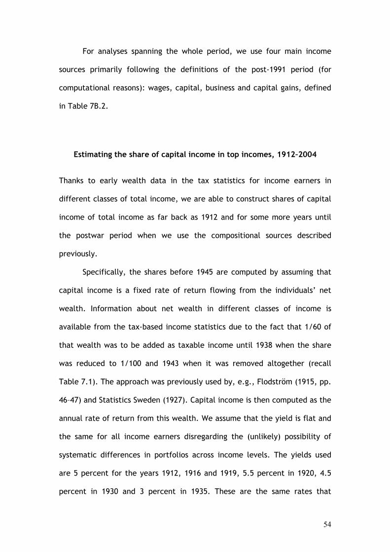
54

For analyses spanning the whole period, we use four main income

sources primarily following the definitions of the post-1991 period (for

computational reasons): wages, capital, business and capital gains, defined

in Table 7B.2.

Estimating the share of capital income in top incomes, 1912–2004

Thanks to early wealth data in the tax statistics for income earners in

different classes of total income, we are able to construct shares of capital

income of total income as far back as 1912 and for some more years until

the postwar period when we use the compositional sources described

previously.

Specifically, the shares before 1945 are computed by assuming that

capital income is a fixed rate of return flowing from the individuals�’ net

wealth. Information about net wealth in different classes of income is

available from the tax-based income statistics due to the fact that 1/60 of

that wealth was to be added as taxable income until 1938 when the share

was reduced to 1/100 and 1943 when it was removed altogether (recall

Table 7.1). The approach was previously used by, e.g., Flodström (1915, pp.

46�–47) and Statistics Sweden (1927). Capital income is then computed as the

annual rate of return from this wealth. We assume that the yield is flat and

the same for all income earners disregarding the (unlikely) possibility of

systematic differences in portfolios across income levels. The yields used

are 5 percent for the years 1912, 1916 and 1919, 5.5 percent in 1920, 4.5

percent in 1930 and 3 percent in 1935. These are the same rates that

55

Flodström and Statistics Sweden use (except for 1920 when they use 5

percent).61 Unlike them, however, we can also motivate our choice of these

rates by referring to three other reference interest rates from the same

particular years. Specifically, the yearly averages of the minimum lending

rate (diskontot) set by the Swedish central bank, the average deposit rate

at Swedish savings banks and the effective Swedish Government bond yield

were in 1912: 4.81, 4.35 and 4.80; in 1916: 5.23, 4.76 and 5.09; in 1919:

6.38, 5.08 and 5.71; in 1920: 6.92, 5.16 and 7.00; in 1930: 3.71, 5.22 and

4.18; and in 1935: 2.50, 3.59 (in 1933) and 3.30 (Svensk Sparbankstidskrift

1934, p. 825). However, Östlind (1945, p. 261) shows numbers of effective

yields of stock exchange-listed stocks during the First World War being

somewhat lower that what we use (4.0 percent for 1916). At the same time,

Beije (1946, pp. 64�–87) shows the market yields of new corporate bond

issues during 1912�–1920 more in line with the ones we use. Finally, the share

of capital income of total income across the various top fractiles is

computed using Pareto interpolation in the same way as in the rest of the

compositional analysis.

Realized capital gains and the identity of top income earners, 1991–2004

One problem with using aggregate income statistics ordered in classes of

total income is that we have problems assessing the true distributional

effects of capital gains income. In short, we do not wish to have our top

61 Unfortunately, no income data were collected in the Census of 1940, so we have no information about wealth shares in different classes of income.

56

total income earners being populated by low wage income earners selling

their house or some old bonds and thereby jumping from the 50th to the

99th percentile.62

A simple way to at least rule out some of the ambiguity is to use the

tabulations by Statistics Sweden of average gross capital gains income (i.e.,

before deductions against interest payments or capital losses) in classes of

earned income, from 1991 onwards. Since the compositional analysis above

showed that business income is only a minimal part of earned income during

this period even for top total income earners, earned income in practice

means wages and salaries. The results of this exercise are shown in Figure

7B.1, where the distributions of realized capital gains are plotted across

classes of labor income for each year in 1991�–2004. Apparently average

capital gains are highest for those who also earn the most, i.e., at least for

this late subperiod of the study we find no support for the hypothesis that

realizations of capital gains create a large turnover of people in our income

distribution and that a constantly significant share of top income earners is

low wage income earners.

Concepts of tax units

The Swedish income statistics have used two main definitions of tax units

over the twentieth century. Before 1951, the tax unit is the family, meaning

married couples or single households, both with any under-aged resident

children. After 1951, the tax unit is the individual. On top of these main

62 This has previously been shown by Saez and Veall (2005) not to be the case among top income earners in Canada.

57

types, there were some minor changes mainly during the latter period which

are discussed in this section.

Income earners (tax units), 1903�–1950: Income earners in the Swedish

income statistics refer to physical persons who lived in Sweden during the

income year and who also filed a personal tax return.63 The Swedish income

statistics was family-based until 1950, which meant that families with at

least one income earner earning more than the lowest taxable income

threshold should file one tax return. Married couples filed a joint tax return.

Income earners (tax units), 1951�–2006: For the period 1951�–2006, the

Swedish income statistics changed to being individual-based, meaning that

individual tax returns form the basis for the income distribution data that

we have used in this study. It should be noted that the definition of income

earners according to published income statistics is typically, but not always,

identical with the contemporaneous tax legislation. In particular, although

the income statistics switched from using households to individuals in 1951,

the Swedish tax system continued taxing families until 1971. But the

transition was gradual between 1954 and 1971. Before 1954 the wife�’s

income was automatically assessed as a part of her husband�’s income.

Between 1954 and 1965 spouses filed separate tax returns after which their

incomes were lumped together and taxed as one tax unit according to a

specific rate of �“joint taxation�” (sambeskattning). Between 1966 and 1970,

the system was further adjusted so that married couples could choose

63 Formally, unfinished death estates and family foundations are also counted as income earners, but they only represent about 1 percent of the total number of income earners.

58

whether to have their income being taxed separately or as one couple

according to a specific scale. Finally, in 1971 the Swedish tax system

changed to being fully individual-based and married couples were thereafter

treated as two income earners.

In the period 1943�–1950 the income statistics followed the tax system

by being household-based, using the total number of filed tax returns as

primary material. Due to processing constraints, however, only a few

variables could be collected for each tax unit and therefore it was decided

to switch to a sample-based system that allowed more background

information to be collected and analyzed. Because of this, Statistics Sweden

decided to start using a nationally representative ten percent sample of the

tax population as basis for its income statistics from the year 1951 onwards.

This basically meant that the income statistics became individual-based

despite still having a family-based tax system since all persons with positive

income had to file an individual tax return regardless of whether they were

eventually taxed jointly with their spouses or parents.64 The ten-percent

sample was drawn from the population of all adults aged 16 years or above

and born on either the 5th, 15th or 25th in each month.65 To avoid sampling

too few high income earners, these groups were fully sampled.66 This is, of

64 The switch to using a population sample followed the instructions of a governmental statute (kungörelse den 21 december 1951, No. 832). 65 Having in fact 365.25 days calendar year, the chosen sample was actually smaller than 10 percent of the population and instead of multiplying each income earner with 10 (for those jointly assessed 5) it should have been 10.146 (and 5.340). As noted by Statistics Sweden in Inkomst och förmögenhet 1968, p. 26 (see Appendix sources), this could have some minor effects on the comparability of the data before and after 1967. 66 The definition of high income was SEK 30,000 or above during 1951�–59 and with income above and SEK 50,000 or above in 1960�–66.

59

course, important in the context of studying top incomes as it means that

we do not have to worry about missing top income earners due to sampling

in this period. The sample-based income statistics lasted until 1967 when

Statistics Sweden returned to basing the income statistics on the complete

tax population with the help of new data processing techniques.

Apart from these major changes in the income earner definitions,

there have been several smaller adjustments and related changes that have

affected the income earner concept. For example, in income years 1972 and

1973 all retirees receiving public pension only (folkpensionärer) were

granted extra deductions so as to avoid paying taxes.67 Another change

happened in 1978 when both employers and employees were required to

report all incomes paid and received, which in itself increased the tax liable

population by a couple of hundred thousand income earners who were most

likely previously avoiding taxes altogether.

The main impact that these changes of tax units have in our study is

on the choice of reference population and how to homogenize this over

time. Details of how we do this are presented below.

Lowest taxable income threshold

Sweden is an outlier internationally in terms of the large share of income

earners that have been obliged to file taxes over the twentieth century.

Figure 7B.2 shows the lowest income level that obliging a tax return (in

Swedish deklarationspliktgräns or “skattestreck”), which is negatively

67 See, e.g., Statistics Sweden, Inkomst och förmögenhet 1973, p. 15.

60

correlated with the number of people included in the tax population. During

the first decade 1903 1910, the level was relatively high, SEK 1,000,

representing between one and two times the overall average income

(reference total income divided by reference total population). Over time,

the level was increased nominally, shown in the right scale in the figure.

Already in 1920, only if one earned a fifth of the average income one had to

file a personal tax return and since the 1950�’s the level has been lowered

even further in relative terms.

It should be noted that although the fairly drastic discrete changes in

the threshold in, e.g., 1911, 1919, 1952, 1962 and 1971, changed the

number of tax filers by several percentage points, this does not affect our

analysis since we always observe the absolute top income earners as well as

the reference total population.68

68 The doubling of the threshold in 1962 was estimated to decrease the number of income earners by about 125,000, representing about 3 percent (Statistics Sweden, Skattetaxeringarna samt fördelningen av inkomst och förmögenhet taxeringsåret 1963, p. 21).

61

APPENDIX 7C: CONSTRUCTION OF REFERENCE TOTALS

Here we explain in greater detail exactly how our reference totals have

been constructed. The different reference totals are used to test the

robustness of our series to the choice of reference total. The reference

totals for tax units and income, 1903-2006, are shown in Table 7C.1.

Reference total population

As described above, there has been one major change in Swedish tax

legislation in the Twentieth Century which has fundamentally changed the

concept of tax unit, namely the 1970 tax reform shift from a family based

tax unit to an individually based concept. In terms of tax statistics,

however, this change occurred (at least to some extent) already in 1951.

Before this tax statistics were based on the entire tax population and figures

referred to �“tax units�” i.e. individuals as well as married couples counted as

one income earner.69 Before 1951 the obvious reference population is

therefore the adult population (which we take to be everybody aged 16 or

above) less married women (since a married women formed one tax unit

together with her husband). After 1951, however, statistics changed to

being based on a representative sample (ten percent) of the population with

married couples, where both had income, now treated as two income

earners in the statistics even though they were still taxed as one unit. The

problem is that in cases where the women did not work, or had low income,

she was not necessarily counted. This means that income statistics between

69 Note that this is the case for tax statistics before 1951 but not income figures in the Census (Folkräkningen).

62

1951 and 1971 when the individually based system was fully introduced (for

labor income, tax on capital income remained family based) is a mix

between a family based system and an individually based system including

some women (those with substantial income) but not all. Starting 1971, the

reference total is again relatively unambiguous, now obviously being the

adult population.

Apart from the quantitatively more substantial decisions discussed

above there are a number of smaller adjustments which can be considered.

Over the course of a year individuals move in and out of the country, some

die, some turn 16 after the population count but before taxes are filed, etc.

Based on recent years when we believe that the coverage in the tax

statistics is close to complete we have concluded that correcting for deaths

is most important. The tax statistics before 1951 contain tax returns for

those who died during the previous year (the income year), in the period

1951-1973 these are not present in our data, but from 1974 and onwards

they are again part of the statistics. We have therefore added deaths to our

reference total for the population before 1951 and after 1973.70 For these

periods we therefore add the number of deaths during the year when

calculating the reference total population.

In terms of choosing the appropriate reference population the period

1903�–2006 can, hence, be divided into the following three periods: 1) 1903�–

70 To be precise, deaths are not in the statistics 1951-1966 (though they are taxed) while they are separately accounted for in the period 1967-1973 and hence we can exclude them from our tables. References for the treatment of deaths are e.g.: for the period before 1951, Statistics Sweden, Inkomst och förmögenhet 1969, p. 11, for the period 1951-1966, Statistics Sweden, Skattetaxeringarna…1966, p. 32, for the period 1967-1973 Statistics Sweden, Inkomst och förmögenhet 1969, p. 13-15, 20-21, and after 1974 Statistics Sweden,SCB SM N 1976:4 (p.2) and SCB OE 21 SM 0501.

63

1950, the total population aged 16 or above minus married women, 2) 1951�–

1970, the total population aged 16 or above minus women likely to be

excluded in the statistics, 3) 1971�–2006, the total population aged 16 or

above.

For the period 1903-1950 the reference total population is:

The population aged 16- (from Statistics Sweden, Population

statistics, SCB Programmet för

befolkningsstatistik)

married women (from Statistics Sweden, Statistical Yearbook

of Sweden, Statistisk Årsbok, various years)

+ deaths during the year (from Statistics Sweden, Statistical Yearbook

of Sweden, Statistisk Årsbok, various years)

For the period 1951-1971 our preferred reference total population is:

The population aged 16- (from Statistics Sweden, Population

statistics, SCB Programmet för

befolkningsstatistik)

married women (no/low inc) Edvinsson (2005, p. 140) reports data on men

and women in paid work and labels married

women not in paid work �“housewives�”. Part

of this group does have income anyway so

we subtract a declining share of

�“housewives�” in the period 1951-1967 (based

64

on smoothing shifts in the ratio between the

number of tax returns and the reference

population, as well as the income shares.71

In 1967 (when individual taxation became

voluntary) the deducted share shifts more

drastically (as does the number of income

earners in the statistics) and in the period

1967 to 1970 the remaining share of

�“housewives�” are subtracted.

For the period 1972-2006 the preferred reference total population is:

The population aged 16- (from Statistics Sweden, Population

statistics, SCB Programmet för

befolkningsstatistik)

+ deaths during the year (added after 1973 since they reappear in the

statistics in 1974, from Statistics Sweden,

Statistical Yearbook of Sweden, Statistisk

Årsbok, various years)

To check the robustness of our results we have calculated a number

of alternatives which differ mainly in the period 1951-1971. These are 71 We start by subtracting 60 percent of married women (which is about 75% of the housewives) and then decrease this share with about 2 percentage points per year until 1967 (as this is about the rate at which the ratio of housewives to married women changes over this period) and then allow for a larger shift between 1966 and 1967 when (judging from the upward jump in the number of tax returns) the number of women with own reported income increased more.

65

sometimes not �“alternatives�” in the sense that we may know that they are

clear over-, or underestimations, but rather they serve the purpose of giving

bounds to our estimates.72 Figure 7C.1 shows the population aged 16 and

above, the number of tax returns and the different alternative

specifications. The alternative specifications are the following:

Preferred series = (Pop 16-) Married W + deaths for 1903-

1950, (Pop 16-) (Decreasing share of

women 1951-1971), and from 1967 Pop 16-

, subtracting declining share of housewives

1967-1971 and adding deaths after 73 (1974-

).

Tax units alt 1 = (Pop 16-) Married W for 1903-1950, and

(Pop 16-) from 1951.

Tax units alt 2 = (Pop 16-) Married W for 1903-1950, (Pop

16-) Housewives for 1951-1966, and (Pop

16-) from 1967.

Tax units alt 3 = (Pop 16-) Married W + Deaths for 1903-

1950, (Pop 16-) Housewives for 1951-1966,

(Pop 16-) Declining share of housewives for

1967-73, (Pop 16-) + Deaths for 1974

onwards.

72 Only Tax units 3 is really an alternative. Here we subtract all housewives in the period 1951-1967.

66

Looking at the behavior of the ratio between the number of tax returns and

our reference series, especially around the critical years when there are

changes in the definition of tax unit, i.e., 1951, 1967 and 1971, indicates

which series seem best. Put simply, we do not want there to be any sudden

jumps in the ratio unless there are underlying real changes in the tax base.

To exemplify, in 1919 the tax threshold was dropped from SEK 800 to SEK

600 leading to a real major expansion of the tax base. Here we expect the

ratio to go up sharply. In 1951, however, the change was only in the type of

statistics, not in the actual underlying number of tax eligible individuals

(units), so here we should not expect a break in the ratio. To the extent

that the number of returns increase this should be compensated by an

increase in the reference total. At the same time, we do not, of course,

wish to make ad hoc adjustments to keep the ratio fixed, since there are

also real changes in the number of tax filers. Figure 7C.2 shows the ratio

between the number of tax returns and our preferred series with indications

of critical breaks.

Reference total income

In constructing our reference total income we have used three basic

approaches. The first two are based on that we can arrive at the �“Preferred

Total Income Definition�” either by 1) starting with �“Total Personal Sector

Income�” and deducting items not included in our preferred definition, or 2)

by starting from the �“Tax Statistics Income�” and adding items not included

in the tax base and income estimates for individuals not included in the tax

statistics. The third - which is mainly included as a point of reference - is

67

based on the assumption that our preferred income total can be

approximated as a fixed share of GDP.

Starting with the first approach, we need homogenous estimates of

�“Total Personal Sector Income�” from which we want to deduct items not

included in our preferred definition of total income. The best homogenous

National Accounts series which span the whole period which we study are

those by Edvinsson (2005). These, however, contain only aggregate series

for Wages and salaries of employees (including social benefits) and Imputed

labor income of self-employed (including social benefits). To these we have

added aggregate capital income and property income reported in the tax

statistics giving us an estimate of �“Personal sector total income�”.73 This,

hence, becomes:

Wages and salaries of employees (including social

benefits), from Edvinsson, 2005

+ Imputed labor income of self-employed (incl. social

benefits) (from Edvinsson, 2005)

+ individual capital income (from Taxeringarna…, 1922-

1988, and corresponding sources thereafter, and

estimated before 1922).

+ individual property income(same as for capital income

above)

= Estimated �“Personal sector total income�”

73 These are available from the aggregate taxation statistics Taxering till inkomst- och förmögenhet 1922-1988, for the years before we add shares based on the observations 1922, and after 1988 we add the corresponding figures in the new tax statistics.

68

This estimate fluctuates around 0.7 times GDP (calculated from the

expenditure side, reported in Edvinsson 2005) with a standard deviation of

0.03.

Starting from the tax statistics income we use the following method

to get at our preferred reference total for income:

Tax statistics income (the aggregates from the same

sources as the income statistics described above,

sometimes corrected for wealth shares)

+ items not included in the tax base (we make the

assumption that all important sources of income

including certain social security benefits are

included in the tax base after 1974 (hence

abstracting from child allowances, allmänt

barnbidrag, and study grants, studiebidrag, which

are tax free) and add aggregate government

expenditures for unemployment benefits

(arbetslöshetsersättning), payments for sick leave

(sjukpenning) and payments for mothers

(moderskapsförsäkring, which in 1974 was replaced

by �“parenthood insurance�”, föräldrarförsäkring,

which was taxed) based on figures in the Statistical

Yearbook of Sweden from 1948- (before they are not

listed but can be assumed to be a small share).

69

+ estimated income for �“non-filers�” (in our preferred

specification we take (reference population - tax

filers) x (0,8 times the tax threshold). As an

alternative specification we use 0.25 times the

average income of tax filers).

= �“Preferred reference total�” (starting from the tax

statistics income)

Figure 7C.3 shows the alternative specifications over the whole period as

shares of GDP, as well as in relation to 0.63 times GDP. What we can say

with some certainty is that the estimate of �“Personal sector total income�” is

an over estimate of our preferred reference total. We can also say with

some certainty that at least since 1974 the tax statistics income is relatively

close to our preferred reference total since most people file taxes and

everything we wish to include as income is included in the tax base. We can

also note that in the period 1930-1990 our �“Preferred reference total�”

calculated starting with the tax statistics income follows the estimated

�“personal sector total income very closely. In fact, taking 0.89 times the

latter, yields numbers which follow the former with very small deviations.74

We also note that for the early years (1903-1920) imputing 0.8 times the

threshold (or 0.25 times average income) clearly yields over estimates of

reference income. This is to be expected since when most individuals are

below the threshold small changes in assumptions about their average

74 The standard deviation is 0.02 and the maximum deviation is 0.05.

70

income make a big difference and at this point in time the average income

amongst tax payers was certainly much higher then later implying that

imputing similar shares to non-filers as later means overestimating their

income a lot.

Given the behavior of these series we have chosen to use 0.89 times

our estimated �“personal sector total income�” as our reference total for the

period 1903-1942 and then (as tax statistics become yearly) our calculated

reference total income starting with tax statistics income. As with the

reference total population we have calculated top income shares using a

number of alternatives as well.

Sensitivity of using different reference totals

Using different reference totals can potentially have an important impact on

the income shares. For some single years, such as the spike in top income

shares in 1916, the difference can be up to five percentage points between

the alternative that gives the lowest and highest estimate respectively. For

some periods, such as in the 1950s when the treatment of women in the

statistics is unclear, the variation can be up to 3 percentage points over

some periods. Overall, however, the main trends in the results are robust to

which alternative is chosen. Figure 7C.4 shows the variation in the P90-95

and P99-100 shares including alternatives which are likely to give upper and

lower bounds for the series. The three first alternatives keep our preferred

population total and varies the income total, while the following four

alternatives change the population total but keep our preferred income

71

total. As the figure shows the beginning of the century, especially the peak

in 1916, and the period 1951-1971 when the treatment of working women is

unclear in the statistics, are the periods with the broadest bands. Overall,

however, the main trends in the results are robust to which alternative is

chosen.

Sensitivity of using individuals or households as tax units

Our income series are computed from the tax returns-based income

statistics for most years, and as we described above this implies that we use

two different concepts of income earners over the twentieth century.

Before 1951, the income earner in our data is the household (or family),

i.e., married couples with, or without, children, single men 16 years and

older, and single women 16 years or older. From 1951 onwards, our income

earner is the individual, meaning all men and women 16 years or older.

Hence, while we in the first period count married couples as one income

earner, they are counted as two income earners in the latter period.

This section offers some partial explorations of how this switch of

income earner concept may influence the overall results of our study. As our

historical data were chosen largely due to availability constraints, we

cannot make a fully-fledged comparison as there are simply no parallel

datasets based on tax data available. What we can do, however, is to

compare our family-based series with the series in which individuals are the

basis. This can be done from the years from which we use the Census

72

material (the years 1920, 1930, 1935 (partial census), 1945 (partial census),

and 1950) when the primary material is individual-based but adjusted by us

and others (especially Bentzel, 1952) to be consistent with the family-based

series from the years before 1920 and in between the other years (1934 and

1937).

Figure 7C.5 shows the income shares of the top fractiles (from top 10

percent to the top 0.05 percent). Solid lines represent our main family-

based income series used in our analysis (called �“Family�”) whereas the

broken lines are the unadjusted, individual-based census series (called

�“Individual�”). Note that since we use different concepts of income earners

in the two cases, we must also use two different reference total populations

to calculate the correct population shares. In our family-based series, we

use the adult population 16 years and above minus married women and in

the individual-based series the adult population 16 years and above is used.

For this reason, the level of the shares may not be fully corresponding to

each other although as Figure 7C.5 shows they as a matter of fact are to

quite some extent. As for the changes in shares over the period, they are

pretty much coinciding in all cases for all fractiles, and importantly there is

no systematic tendency in some direction of either series. For example,

whereas the individual-based series produce slightly larger declines between

1935 and 1950 for the top 10 percent to top 0.5 percent income earners, the

family-based series do it for the top 0.1 to top 0.05 percent fractiles.

Altogether, we feel confident with our choice of income earner concepts

and have not found any systematic biases when contrasting them with

alternative definitions.

73

Age adjustments and effects of censoring the youngest income earners

Similar to previous studies of top incomes, we impose a lower age bound on

the analyzed tax population in order to ensure that we do not include

under-aged children in the analysis and that the series are conceptually

consistent over the years. Specifically, we impose an age cutoff at 16 years,

which means that we include all income earners aged 16 and above. We

choose this age as it since long has marked the beginning of a person�’s

period in life after completing the compulsory Swedish secondary education.

Furthermore, the 16 year-olds were the youngest ones sampled by Statistics

Sweden in the income statistics during 1951�–1966 and ever since the late

1970�’s it was also the lowest reported age in the published income

statistics. For robustness purposes, however, we have also run our entire

analysis using income earners aged 20 and older, but the results are

qualitatively the same.75 The finding that the exact choice of age cutoff is

not important for the estimated trends in top income shares has also been

found by Atkinson and Leigh (2007b).

In practice, our age cutoff means that we subtract the number of

income earners aged 15 or less from our reference total population and from

the main top income series but not from the reference income total. The

reason is that we lack specific data on their incomes. However, it turns out

75 For some postwar years, Statistics Sweden used a different lowest age cutoff in its reported age-income distributions than 16. During 1957�–1966 it was 17 and during 1971�–1977 it was 18. We interpolate the shares of our (unobserved) 0�–15 group based on the continuously observed 0�–19 group. This bridging of the series appears to be of minor importance.

74

that their incomes are quite marginal and leaving them in the reference

income does not influence the results of our study.

In Figure 7C.6, we reinforce the aforementioned result that removing

children between 0 and 15 years old from our analyzed tax population

makes no difference. In fact, the tax reform implemented changes which

made almost all children with some bank holdings part of the tax population

why if we would not have made any such age adjustments we would have

run into great difficulties. The figure shows that throughout the postwar

period these youngsters had quite marginal incomes relative to the rest of

the population, being about 0.1 percent. Their share of the number of tax

units in the tax population increased disproportionately, however, in 1978

and 1992. In 1978, new tax collection routines required employers to submit

income statements (kontrolluppgifter) for all employees, which implied that

a number of children working extra a few weeks during the summer holidays

were included in the tax population. More importantly, after the tax reform

in 1991 there was a drastic increase in the share of young income earners.

This was directly related to new rules in the reform which stated that

capital income over SEK 100 was made taxable. As a consequence, almost

one million children, roughly one ninth of the entire Swedish population,

became tax units overnight.76 In other words, by excluding the youngest

income earners we avoid some unwarranted heterogeneity in the income

earner shares caused by the tax reform of 1990�–1991.

76 Formally, the new rules were in practice already in 1991 but in that year�’s income statistics Statistics Sweden made an adjustment to exclude the new bulk of very young income earners. They excluded all income earners below 18 years of age with labor income less than SEK 12,000 (Statistics Sweden, Inkomst- och skattestatistik 1991, Be 20 SM 9301, p. 9).

75

Figure 7.1 The top 10 percent income share in Sweden (with and without capital gains), 1903 2006.

20

25

30

35

40

45

50

55

1900 1910 1920 1930 1940 1950 1960 1970 1980 1990 2000

Sh

are

of

inco

me (

%)

P90-100 incl. cap. gains

P90-100 excl. cap. gains

Source: Column 1 in Appendix tables 7A.2 and 7A.3, respectively.

76

Figure 7.2 The P90 95, P95 99 and P99 100 (top 1 percent) income

shares in Sweden (with and without capital gains), 1903 2006.

2

6

10

14

18

22

26

30

1900 1910 1920 1930 1940 1950 1960 1970 1980 1990 2000

Sh

are

of

inco

me (

%)

P90-95 incl. cap. gains P90-95 excl. cap. gains

P95-99 incl. cap. gains P95-99 excl. cap. gains

P99-100 incl. cap. gains P99-100 excl. cap. gains

Source: Columns 3, 8 and 9 in Appendix tables 7A.2 and 7A.3, respectively.

77

Figure 7.3 The top 0.01 percent income share in Sweden (with and without capital gains), 1903 2004.

0

1

2

3

4

5

6

1900 1910 1920 1930 1940 1950 1960 1970 1980 1990 2000

Sh

are

of

inco

me (

%)

P99.99-100 incl. cap. gains

P99.99-100 excl. cap. gains

Source: Column 7 in Appendix tables 7A.2 and 7A.3, respectively.

78

Figure 7.4 Income composition within the top decile in Sweden 1945, 1978 and 2004

1945

0%

10%

20%

30%

40%

50%

60%

70%

80%

90%

100%

P90-95 P95-99 P99-99.5 P99.5-99.9 P99.9-99.95 P99.95-99.99

P99.99-100

Sh

are

of

tota

l in

com

e

Wages CG Business CG Capital CG Capital gainsWages Business Capital

1978

0%

10%

20%

30%

40%

50%

60%

70%

80%

90%

100%

P90-95 P95-99 P99-99.5 P99.5-99.9 P99.9-99.95 P99.95-99.99 P99.99-100

Sh

are

of

tota

l in

com

e

Wages CG Business CG Capital CG Capital gainsWages Business Capital

2004

0%

10%

20%

30%

40%

50%

60%

70%

80%

90%

100%

P90-95 P95-99 P99-99.5 P99.5-99.9 P99.9-99.95 P99.95-99.99 P99.99-100

Sh

are

of

tota

l in

com

e

Wages (CG) Business (CG) Capital (CG) Capital gainsWages Business Capital

79

Figure 7.5 The evolution of capital income shares in Sweden (excluding and including capital gains) within the top decile, 1912�–2004.

Capital share of total income excluding capital gains

0%

10%

20%

30%

40%

50%

60%

70%

1912 1922 1932 1942 1952 1962 1972 1982 1992 2002Cap

ital

share

of

tota

l in

com

e (

excl

. cap

ital

gain

s)

P90- 99 P99- 99.9 P99.9- 99.99 P99.99- 100

Capital share of total income including realized capital gains

0%

10%

20%

30%

40%

50%

60%

70%

80%

90%

100%

1912 1922 1932 1942 1952 1962 1972 1982 1992 2002

Cap

ital sh

are

of

tota

l in

com

e (

incl

. ca

pit

al g

ain

s)

P90- 99 P99- 99.9 P99.9- 99.99 P99.99- 100

80

Figure 7.6 Total income shares vs. market income shares in Sweden of P99�–100, 1950-2006.

3

4

5

6

7

8

9

10

11

12

13

1950 1955 1960 1965 1970 1975 1980 1985 1990 1995 2000

Sh

are

of

inco

me (

%)

Total income (incl. cap.gains) P99-100 Total income (excl. cap.gains) P99-100

Market income (incl. cap.gains) P99-100 Market income (excl. cap.gains) P99-100

81

Figure 7.7 The capital share of value added as a share of GDP and the top 1 percent income share in Sweden, 1903�–2003

0.15

0.20

0.25

0.30

0.35

0.40

0.45

0.50

1900 1910 1920 1930 1940 1950 1960 1970 1980 1990 2000

Gro

ss S

urp

lus/

GD

P

0

5

10

15

20

25

30

Sh

are

of

inco

me (

%)

Capital share of value added/GDP

P99-100

Sources: Data on the capital share of value added and GDP by activity come from Edvinsson (2005). Top income percentile shares come from Appendix table 7A.2 column 1.

82

Figure 7.8 Wealth in top income and wealth fractiles in Sweden, 1908�–2004.

0

10

20

30

40

50

60

70

1900 1910 1920 1930 1940 1950 1960 1970 1980 1990 2000

Wealt

h s

hare

(%

)

2

6

10

14

18

22

26

30

Inco

me s

hare

(%

)

P99-100 (income distribution) P90-99 (income distribution)

P99-100 (wealth distribution) P90-99 (wealth distribution)

P99-100 (income distribution, right axis) P90-99 (income distribution, right axis)

Source: Authors�’ own calculations.

Note: the circles relate to wealth shares (left hand scale) of units ranked by income.

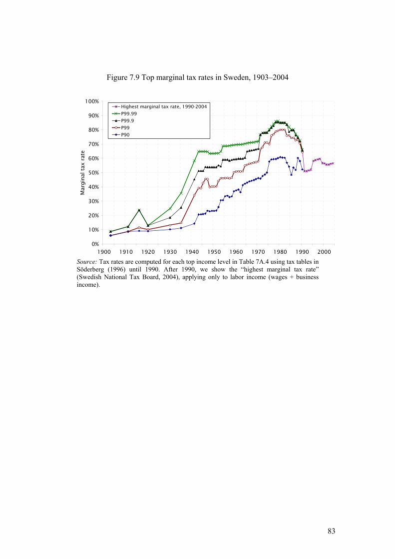
83

Figure 7.9 Top marginal tax rates in Sweden, 1903�–2004

0%

10%

20%

30%

40%

50%

60%

70%

80%

90%

100%

1900 1910 1920 1930 1940 1950 1960 1970 1980 1990 2000

Mar

gin

al t

ax r

ate

Highest marginal tax rate, 1990-2004

P99.99

P99.9

P99

P90

Source: Tax rates are computed for each top income level in Table 7A.4 using tax tables in Söderberg (1996) until 1990. After 1990, we show the �“highest marginal tax rate�” (Swedish National Tax Board, 2004), applying only to labor income (wages + business income).

84

Figure 7.10 Capital gains in some top income fractiles and real stock prices in Sweden, 1967�–2004.

0

5

10

15

20

25

30

1967 1971 1975 1979 1983 1987 1991 1995 1999 2003

Cap

ital

gain

s i

nco

me (

bil

lio

n S

EK

)

0

50

100

150

200

250

300

350

Sto

ck p

rice

in

dex (

19

95

= 1

00

)

Capital gains earned in P90-99

Capital gains earned in P99.9-99.99

Capital gains earned in P99.99-100

Swedish real stock prices (yearly average)

Note: Stock prices are yearly averages of end-of-month prices up to 1979 and daily closing prices thereafter of Affärsvärldens Generalindex (http://www.affarsvarlden.se), deflated with monthly CPI (monthly averages).

85

Figure 7.11 Income shares of the top percentile in Western countries, 1903�–2004.

0

5

10

15

20

25

30

1900 1910 1920 1930 1940 1950 1960 1970 1980 1990 2000

Sh

are

of

tota

l in

com

e (

%)

USA UK

Canada France

Australia Sweden (incl. cap. gains)

Netherlands Sweden (excl. cap. gains)

Notes and Sources: Australia (Atkinson and Leigh, 2006), Canada (Saez and Veall, 2005), France (Piketty, 2003), Netherlands and the UK (Atkinson and Salverda, 2005) and the US (Piketty and Saez, 2003).

86

Figure 7B.1 Average gross capital gains income in classes of earned income in

Sweden, 1991�–2003.

0

500,000

1,000,000

1,500,000

2,000,000

2,500,000

0 80,000 180,000 280,000 1,000,000

Classes of earned income (wages + business income)

Ave

rage

cap

ital

gai

ns

inco

me

1991199219931994199519961997199819992000200120022003

87

Figure 7B.2 Lowest taxable income and its share of average total income on Sweden,

1903�–2003.

0

2000

4000

6000

8000

10000

12000

14000

16000

18000

1903 1913 1923 1933 1943 1953 1963 1973 1983 1993 2003

Low

est

taxab

le inco

me

(SEK

, cu

rren

t pri

ces)

0

0.5

1

1.5

2

2.5

3

3.5

4

Rat

io b

etw

een low

est

taxab

le inco

me

and

av

erag

e in

com

e

Lowest taxable income (left scale)Lowest taxable income divided by Average total income (right scale)

88

Figure 7C.1 Tax returns and alternative population totals in Sweden, 1903�–2006.

1

2

3

4

5

6

7

8

1900 1910 1920 1930 1940 1950 1960 1970 1980 1990 2000

Nu

mb

er

of

tax u

nit

s/t

ax r

etu

rns (

mil

lio

ns)

Tax returns (Pop 16-) Tax units (preferrred) Tax units 1 Tax units 2 Tax units 3 Pop 16-

1951: Shift in income statistics leading to the inclusion of married women with own income

1967: Shift in tax statistics, individually based taxation is introduced on a voluntary basis

1978: Employers start sending income statements to the tax authorities

1918: Lowest taxable income down from 800 SEK to 600 SEK (Almost doubled the number of returns between 1916 and 1919)

89

Figure 7C.2 Ratios between tax returns and alternative reference populations in

Sweden, 1903�–2006.

0.00

0.20

0.40

0.60

0.80

1.00

1.20

1900 1910 1920 1930 1940 1950 1960 1970 1980 1990 2000

(N. ret 16-)/TU1 (N. ret 16-)/TU2 (N. ret 16-)/TU3 (N. ret 16-)/Preferred series

90

Figure 7C.3 Different reference totals for income as shares of GDP in Sweden, 1903�–

2004.

0.2

0.3

0.4

0.5

0.6

0.7

0.8

0.9

1

1.1

1903 1913 1923 1933 1943 1953 1963 1973 1983 1993

Pref RefTotInc/GDP (0.89xTotPersInc)/GDP

(TaxStatInc+NonTaxedInc+0.8xthreshold)/GDP TaxStatInc+NonTaxedInc+0.25xavgtaxpayerinc)/GDP

Total Personal Sector Income 0.63xGDP

91

Figure 7C.4 P90-95 and P99 series in Sweden using different reference totals.

0

5

10

15

20

25

30

1903 1913 1923 1933 1943 1953 1963 1973 1983 1993 2003

P90- 95 P99 P90- 95:2 P99:2 P90- 95:3 P99:3 P90- 95:4

P99:4 P90- 95:5 P99:5 P90- 95:6 P99:6 P90- 95:7 P99:7

92

Figure 7C.5 Sensitivity of Census-based top income shares in Sweden when switching

tax unit definitions between individual and household

0

5

10

15

20

25

30

35

40

45

1920 1925 1930 1935 1940 1945 1950

Sh

are

of

tota

l in

com

e (

%)

P90-100 Individuals P90-100 Households P95-100 Individuals

P95-100 Households P99-100 Individuals P99-100 Households

P99.5-100 Individuals P99.5-100 Households P99.9-100 Individuals

P99.9-100 Households P99.95-100 Individuals P99.95-100 Households

P99.95-100

P95-100

P99.9-100

P99.5-100

P99-100

P90-100

93

Figure 7C.6 Shares of population and total income of children under 16 years old in Sweden, 1951�–2003.

0%

2%

4%

6%

8%

10%

12%

14%

1951 1958 1965 1972 1979 1986 1993 2000

Sh

are

of

all

in

com

e e

arn

ers

or

tota

l in

com

e

Childens' share of tax population(before age adjustments)

Childens' share of total income(before age adjustments)

94

Table 7.1 Definitions and adjustments of the income data and reference totals in Sweden

Income years

Income concept appearing in data sources

[Swedish term] Adjustments

Reference total income

Reference total population

1903–1910

Taxable income [till statlig inkomstskatt taxerad

inkomst]. Bascially �“Total income�”.

1911–1942

Taxable amount [Taxerat belopp] = Taxable income (see above) + Wealth share (share of taxable personal net wealth) Some taxes.

Removal of wealth shares and after 1920

addition of some municipal

taxes

Share of �“total personal sector income�” (from

National accounts) adding estimates of items not included

in the preferred definition (1903�–

1942)

1943–1950

Adult population (>15 yrs) minus married women

( 1950)

1951–1970

Total income [Sammanräknad

nettoinkomst] = Total (gross) income Deficits

at source

Age adjustment (excluding all <16 years old)

Adult population (>15 yrs) adj. for

women being (partially)

included in the income statistics

(1951�–1970)

1971–1990 Total (gross) income [Sammanräknad inkomst]

Subtracting deficits at

source + Age adjustment

1991–2006 Total income [Summa

förvärvs- och kapitalinkomst]

Age adjustment

Tax statistics income plus

estimates of non-taxed items included in

preferred def. (mainly corrections

for changed tax treatment of

unemployment and sick pay insurance etc. before 1974)

plus estimated incomes of �“non-

filers�” (1943�–)

Adult population (>15 yrs) (1971

)

Note: All concepts are elaborated upon in the Appendix. No age-specific data were available for different income classes until 1951.

95

Table 7.2 Top income thresholds and average incomes in Sweden in 2004.

Thres-hold

Income (incl.

capital gains) in

USD

Income (excl. capital

gains) in USD

Fractiles N tax units (individual

s)

Ave. Income (incl. capital

gains) in USD

Ave. Income (excl. capital gains) in USD

Full tax pop. 7,395,545 27,875 26,801

P90 48,697 46,354 P90–95 369,777 55,021 51,625

P95 61,154 58,123 P95–99 295,822 72,943 73,665

P99 115,294 79,416 P99–99.9 66,560 156,915 118,619

P99.9 298,488 240,706 P99.9–99.99 6,656 497,511 344,027

P99.99 1,218,259 685,380 P99.99–100 740 3,336,038 1,554,507 Note: The calculations are based on income tax data, with income defined as total income (excluding and including capital gains, ranked in classes of total income including capital gains) before individual taxes expressed in 2004 USD converted from Swedish kronor (SEK) using the 2004 average exchange rate of 7.36SEK/USD.

96

Table 7.3 Decomposition of changes in top income shares in Sweden into wage-, capital- and other incomes over three sub-periods between 1912 and 1980.

Percentage change in Total income shares With contribution by... Wages Capital income Business income

P90�–95 6.1 8.8 �–1.2 �–1.4 P95�–99 �–9.4 �–1.8 �–6.3 �–1.4 P99�–100 �–41.1 �–9.1 �–23.8 �–8.2

1912–1935

P99.9�–100 �–53.0 �–7.2 �–35.2 �–10.6 P90�–95 0.3 �–2.6 �–4.6 7.5 P95�–99 �–10.0 �–9.9 �–7.6 7.4 P99�–100 �–38.6 �–16.7 �–19.4 �–2.5

1935–1951

P99.9�–100 �–56.2 �–21.8 �–27.0 �–7.3 P90�–95 �–2.5 11.9 0.7 �–15.1 P95�–99 �–11.7 11.6 �–1.5 �–21.8 P99�–100 �–36.1 �–6.6 �–4.9 �–24.6

1951–1980

P99.9�–100 �–49.5 �–19.8 �–5.0 �–24.7 Note: Calculations are based on tax returns data from 1945 onwards and Census data from 1920, 1930, 1935 and 1945, including estimates of returns to wealth. Business income is calculated as a residual prior to 1951.

97

Table 7.4 Contribution of changes in the top income earners�’ wealth shares on their income shares in Sweden, 1911�–1991.

Period Change in P99 income share*

(percentage points)

Change resulting from changes in wealth (assuming factor share

0.3, percentage points)

Change resulting from changes in wealth (calculated factor shares,

percentage points)

1911–12 1.36 0.52 0.92 1912–16 7.12 4.36 7.76 1916–19 �–11.70 �–2.57 �–5.14 1919–20 �–2.85 �–0.59 �–1.79 1920–30 0.26 �–0.58 �–1.29 1930–34 �–1.80 �–1.86 �–2.01 1934–35 0.37 0.52 0.76 1935–41 �–2.03 �–0.39 �–0.17 1941–51 �–3.21 �–0.64 �–0.60 1951–91 �–1.26 �–1.87 �–2.44 Sources: Own calculations based on income and wealth shares reported above. * Changes based on the series including capital gains. The calculated change in the P99�–100 income share between 1951 and 1991 is based on an average of the share in 1990�–1992 as 1991 is an outlier in the series including capital gains (as discussed in Section 7.3) due to the tax reform.

98

Table 7.5 Marginal tax effects on top incomes in Sweden, 1943�–1990.

Coefficient estimates

Fractile Model

Constant0

�ˆ( ) Elasticity

1�ˆ( )

Trend2

�ˆ( ) Trend2

3�ˆ( ) R2 Pr.>

2

OLS 3.51***

(0.06) 0.07

(0.13) �–0.01 (0.01)

�–0.00 (0.00) 0.79

P90 2SLS

3.53***

(0.04) 0.30*** (0.11)

�–0.00 (0.00)

�–0.00 (0.00) 0.77 0.00

OLS 2.39***

(0.08) 0.27*** (0.10)

�–0.02** (0.01)

0.00** (0.00) 0.88

P99 2SLS

2.41***

(0.05) 0.32*** (0.06)

�–0.02*** (0.00)

0.00*** (0.00) 0.88 0.98

OLS 1.43***

(0.09) 0.53*** (0.08)

�–0.04*** (0.01)

0.00*** (0.00) 0.92

P99.9 2SLS

1.45***

(0.07) 0.58*** (0.07)

�–0.04*** (0.00)

0.00*** (0.00) 0.92 0.87

OLS 0.64***

(0.10) 0.81*** (0.09)

�–0.07*** (0.00)

0.00*** (0.00) 0.91

P99.99 2SLS

0.71***

(0.13) 0.89*** (0.13)

�–0.06*** (0.00)

0.00*** (0.00) 0.91 0.19

Notes: OLS regressions use Newey-West standard errors (with 6 lags). The 2SLS instrument the net-of-tax rate with the ln(1 �– Statutory top marginal tax rate). Tax rates are calculated using laws listed in Söderberg (1996). Pr.> 2 shows p-values from Hausman tests of a difference between OLS and 2SLS. All regressions have 48 observations. *, **, *** denote significance at the 10%-, 5%- and 1%-levels, respectively.

99

Table 7.6 Percentage change in top percentile income shares in Sweden during the Second World War

Percentage change in the top percentile income share in... Period: Sweden Australia Canada France Netherlands UK USA

1939�–1945 �–4.6 �–24.0 �–40.1 �–43.3 �–12.7 �–22.7 �–25.5 1946�–1951 �–27.2 11.4 �–0.9 19.4 �–11.2 �–15.2 �–5.3

Note: For Sweden, we use 1941�–1945 since no data exist for 1939.

100

TABLE 7A.1 LIST OF SOURCES FOR TOTAL INCOMES AND INCOME COMPOSITION IN SWEDEN, 1903–2006.

Year Main source a), b) Tables Pages Series c) 1903 Flodström (1906) 1, 3 1907 Flodström (1909) XI-XII FU 1911 Flodström (1914) 11 FU 1912 Flodström (1915) 13* FU 1916 Statistics Sweden (1921) C, E 21*-27* SOS 1919 Statistics Sweden (1923) C 21* SOS 1920 Statistics Sweden (1927) 21 558-559 SOS 1930 Statistics Sweden (1937) 11 268-269 SOS 1934 SOU 1936:18 10 47 SOS 1935 Statistics Sweden (1940) 21 88-89 1941 Quensel (1944) VIII, IX 22-23, 28 1943 Skattetaxeringarna (1) ... taxeringsåret 1944 L 31* SOS 1944 Skattetaxeringarna (1) ... taxeringsåret 1945 Q 43* SOS 1945 Skattetaxeringarna (1) ... taxeringsåret 1946 P 42* SOS Statistics Sweden (1951), Census of 1945 4 2-3 SOS 1946 Skattetaxeringarna (1) ... taxeringsåret 1947 R 47* SOS 1947 Skattetaxeringarna (1) ... taxeringsåret 1948 V 51* SOS 1948 Skattetaxeringarna (1) ... taxeringsåret 1949 Q 48* SOS 1949 Skattetaxeringarna (2) ... taxeringsåret 1950 R 48* SOS 1950 Skattetaxeringarna (2) ... taxeringsåret 1951 S 51* SOS 1951 Skattetaxeringarna (2) ... taxeringsåret 1952 Å, 8 63*, 26-27 SOS Statistics Sweden (1956), Census of 1950 7 20-21 SOS 1952 Skattetaxeringarna (2) ... taxeringsåret 1953 Z, 8 53º, 26-27 SOS 1953 Skattetaxeringarna (2) ... taxeringsåret 1954 Z, 8 49º, 26-27 SOS 1954 Skattetaxeringarna (2) ... taxeringsåret 1955 Z, 8 47º, 26-27 SOS 1955 Skattetaxeringarna (2) ... taxeringsåret 1956 Z, 8 46º, 28-29 SOS 1956 Skattetaxeringarna (2) ... taxeringsåret 1957 Z, 8 47º, 28-29 SOS 1957 Skattetaxeringarna (2) ... taxeringsåret 1958 Y, 8 47º, 28-29 SOS 1958 Skattetaxeringarna (2) ... taxeringsåret 1959 Å, 8 50º, 34-35 SOS 1959 Skattetaxeringarna (2) ... taxeringsåret 1960 J, 8 28º, 32-33 SOS 1960 Skattetaxeringarna (2) ... taxeringsåret 1961 I, 10 28º, 32-33 SOS 1961 Skattetaxeringarna (3) ... taxeringsåret 1962 I, 10 28º, 34-35 SOS 1962 Skattetaxeringarna (3) ... taxeringsåret 1963 J, 10 29º, 34-35 SOS 1963 Skattetaxeringarna (3) ... taxeringsåret 1964 J, 10 43º, 36-37 SOS 1964 Skattetaxeringarna (3) ... taxeringsåret 1965 K, 10 44º, 36-37 SOS 1965 Skattetaxeringarna (3) ... taxeringsåret 1966 J, 10 43º, 116-117 SOS 1966 Skattetaxeringarna (3) ... taxeringsåret 1967 L, 9 43º, 118-119 SOS 1967 Inkomst och förmögenhet 1967 2, 7 44-45, 58-61 SOS 1968 Inkomst och förmögenhet 1968 2, 7 50-51, 64-67 SOS 1969 Inkomst och förmögenhet 1969 2, 7 50-51, 64-67 SOS 1970 Inkomst och förmögenhet 1970 2, 7 48-49, 62-65 SOS 1971 Inkomst och förmögenhet 1971 3, 12 68-69, 90-93 SOS 1972 Inkomst och förmögenhet 1972 1, 3, 14 54-5, 70-1, 102-05 SOS Inkomst- och förmögenhetsfördelningen 1972 7 19 SM N 1973:941973 Inkomst och förmögenhet 1973 3, 14 68-69, 100-103 SOS

101

1974 Inkomst- och förmögenhetsfördelningen 1974 1, 7 11, 33 SM N 1976:4 1975 Inkomst- och förmögenhetsfördelningen 1975 1, 7 13, 35 SM N 1976:231976 Inkomst- och förmögenhetsfördelningen 1976 1, 7 18, 41, 43 SM N 1977:241977 Inkomst- och förmögenhetsfördelningen 1977 1, 7 22, 46-47 SM N 1978:221978 Inkomst- och förmögenhetsfördelningen 1978 1, 4.1, 4.2 29, 38, 41 SM N 1980:9 1979 Inkomst- och förmögenhetsfördelningen 1979 1, 4.1, 4.2 20, 27, 30 SM N 1981:9.11980 Inkomst- och förmögenhetsfördelningen 1980 1, 4.1, 4.2 7, 14, 17 SM N 1976:4 1981 Inkomst- och förmögenhetsfördelningen 1981 1, 4.1, 4.2 7, 14, 17 SM N 1976:4 1982 Inkomst- och förmögenhetsfördelningen 1982 1, 4.1, 4.2 14, 21, 24 SM Be 1984:6.11983 Inkomst- och förmögenhetsfördelningen 1983 1, 4.1, 4.2 14, 21, 24 Be 20 SM 85011984 Inkomst- och förmögenhetsfördelningen 1984 1, 3.1, 3.2 15, 19, 22 Be 20 SM 86011985 Inkomst- och förmögenhetsfördelningen 1985 1, 2.1, 2.2 15, 18, 21 Be 20 SM 87011986 Inkomst- och förmögenhetsfördelningen 1986 1, 2.1, 2.2 17, 20, 23 Be 20 SM 88011987 Inkomst- och förmögenhetsfördelningen 1987 1, 2.1, 2.2 17, 20, 23 Be 20 SM 89011988 Inkomst- och skattestatistik 1988 1, 2.1, 2.2 16, 19, 22 Be 20 SM 90011989 Inkomst- och skattestatistik 1989 1, 2.1, 2.2 16, 20, 23 Be 20 SM 91011990 Inkomst- och skattestatistik 1990 1, 2.1, 2.2 15, 20, 23 Be 20 SM 92011991�– 2006

Tables with grouped income distributions acquired directly from Statistics Sweden

a) Some publications titles are abbreviated. Skattetaxeringarna (1) = Skattetaxeringarna samt inkomstfördelningen inom yrkesgrupper; Skattetaxeringarna (2) = Skattetaxeringarna samt fördelningen av inkomst och förmögenhet inom yrkesgrupper; Skattetaxeringarna (3) = Skattetaxeringarna samt fördelningen av inkomst och förmögenhet taxeringsåret. b) The publications since 1982 also have the subtitle Totalräknad statistik. c) �“FU�” denotes Finansstatistiska utredningar (Fiscal Surveys) and �“SOS�” Sveriges officiella statistik (Swedish Official Statistics).

102

Table 7A.2 Total income shares (excluding capital gains) in Sweden, 1903-2006

Shares (excl. capital gains income)

P90-100 P95-100 P99-100 P99.5-100 P99.9-100 P99.95-100 P99.99-100 Year (1) (2) (3) (4) (5) (6) (7) 1903 46.79 35.33 26.99 19.16 8.66 6.15 2.79 1904 1905 1906 1907 45.42 36.33 21.46 16.57 8.72 6.47 2.99 1908 1909 1910 1911 43.90 34.11 19.57 15.21 8.11 6.08 3.02 1912 45.59 35.75 20.92 16.29 8.99 6.84 3.55 1913 1914 1915 1916 52.97 43.53 28.04 22.93 13.70 10.60 5.12 1917 1918 1919 41.91 31.23 16.33 11.70 7.33 5.55 2.91 1920 35.83 26.13 13.48 10.16 5.23 3.86 1.84 1921 1922 1923 1924 1925 1926 1927 1928 1929 1930 38.41 27.87 13.74 10.15 4.82 3.45 1.52 1931 1932 1933 1934 38.06 26.73 11.95 8.54 3.83 2.68 1.12 1935 36.18 25.74 12.32 8.98 4.22 2.99 1.21 1936 1937 1938 1939 1940 1941 34.09 23.67 10.29 7.15 3.01 2.06 0.84 1942 1943 35.61 24.48 10.44 7.19 2.99 2.01 0.78 1944 34.84 23.82 10.04 6.89 2.85 1.92 0.77 1945 34.23 23.36 9.77 6.69 2.72 1.82 0.70 1946 34.29 23.52 10.07 6.99 2.91 2.00 0.80

103

1947 32.09 21.43 8.62 5.85 2.35 1.59 0.60 1948 30.77 20.28 7.90 5.31 2.06 1.32 0.50 1949 30.35 19.89 7.64 5.09 1.96 1.29 0.48 1950 30.25 19.80 7.59 5.06 1.94 1.28 0.47 1951 29.84 19.41 7.33 4.91 1.94 1.30 0.51 1952 29.08 18.60 6.80 4.49 1.73 1.15 0.44 1953 29.60 19.01 6.90 4.55 1.75 1.16 0.45 1954 29.21 18.71 6.90 4.57 1.75 1.15 0.44 1955 28.82 18.39 6.78 4.48 1.69 1.11 0.41 1956 28.83 18.20 6.65 4.38 1.64 1.07 0.40 1957 29.21 18.59 6.81 4.47 1.67 1.09 0.40 1958 29.52 18.75 6.81 4.45 1.65 1.07 0.40 1959 30.06 19.18 7.00 4.57 1.69 1.10 0.40 1960 30.35 19.34 6.83 4.41 1.60 1.03 0.37 1961 30.36 19.27 6.77 4.35 1.55 0.99 0.35 1962 30.08 19.03 6.65 4.25 1.50 0.96 0.34 1963 29.95 18.95 6.64 4.25 1.50 0.95 0.33 1964 29.80 18.77 6.50 4.14 1.43 0.90 0.31 1965 29.69 18.67 6.47 4.11 1.42 0.90 0.31 1966 29.58 18.50 6.35 4.02 1.37 0.86 0.29 1967 30.33 19.17 6.55 4.10 1.38 0.86 0.29 1968 30.39 19.21 6.57 4.11 1.39 0.87 0.29 1969 30.02 18.88 6.41 4.01 1.34 0.84 0.28 1970 29.36 18.34 6.16 3.83 1.28 0.79 0.26 1971 28.36 17.59 5.80 3.60 1.19 0.74 0.24 1972 27.89 17.27 5.67 3.51 1.15 0.71 0.23 1973 27.56 17.00 5.57 3.44 1.13 0.70 0.23 1974 27.07 16.58 5.47 3.39 1.12 0.69 0.23 1975 26.38 16.14 5.29 3.28 1.07 0.67 0.23 1976 25.55 15.48 4.95 3.04 0.96 0.59 0.19 1977 24.72 14.91 4.69 2.86 0.83 0.54 0.21 1978 23.99 14.38 4.47 2.70 0.83 0.50 0.18 1979 23.47 13.97 4.25 2.56 0.77 0.49 0.18 1980 22.73 13.44 4.05 2.42 0.74 0.47 0.17 1981 22.40 13.19 3.97 2.38 0.76 0.48 0.19 1982 22.33 13.18 3.98 2.40 0.77 0.49 0.19 1983 22.42 13.29 4.08 2.47 0.81 0.54 0.25 1984 22.30 13.31 4.13 2.52 0.82 0.57 0.25 1985 22.33 13.35 4.12 2.49 0.80 0.56 0.24 1986 22.35 13.39 4.11 2.47 0.77 0.54 0.23 1987 22.54 13.59 4.24 2.55 0.86 0.60 0.26 1988 22.53 13.62 4.38 2.72 0.99 0.70 0.31 1989 22.55 13.68 4.48 2.81 1.07 0.79 0.40 1990 22.75 13.73 4.38 2.72 1.02 0.73 0.34 1991 24.33 15.04 5.10 3.27 1.30 0.89 0.39 1992 24.33 15.04 5.04 3.19 1.22 0.82 0.35 1993 24.63 15.31 5.22 3.33 1.30 0.88 0.37 1994 25.23 15.85 5.53 3.61 1.45 1.00 0.41 1995 24.93 15.54 5.25 3.35 1.31 0.88 0.38 1996 25.56 16.05 5.59 3.69 1.41 0.98 0.40 1997 25.82 16.23 5.72 3.80 1.47 1.03 0.43

104

1998 25.91 16.35 5.87 3.91 1.57 1.09 0.45 1999 26.12 16.52 6.01 4.00 1.62 1.13 0.48 2000 26.72 17.12 5.97 4.43 1.93 1.37 0.61 2001 26.76 17.10 5.95 4.33 1.86 1.32 0.57 2002 26.43 16.77 5.67 4.07 1.69 1.18 0.51 2003 26.12 16.54 5.52 4.02 1.70 1.20 0.58 2004 26.34 16.71 5.72 4.09 1.73 1.22 0.58 2005 26.96 17.33 6.28 4.40 1.91 1.35 0.64 2006 27.30 17.73 6.61 4.73 2.21 1.63 0.83

Table 7A.2 (continued): Total income shares (excluding capital gains) in Sweden, 1903-2006

Shares (excl. capital gains income)

P90-95 P95-99 P99-99.5 P99.5-99.9 P99.9-99.95 P99.95-99.99Year (1) (2) (3) (4) (5) (6) 1903 11.58 8.41 7.90 10.64 2.55 3.43 1904 1905 1906 1907 9.19 15.03 4.92 7.94 2.29 3.54 1908 1909 1910 1911 9.90 14.70 4.38 7.19 2.06 3.11 1912 9.95 14.99 4.66 7.39 2.18 3.36 1913 1914 1915 1916 9.54 15.66 5.13 9.33 3.15 5.58 1917 1918 1919 10.81 15.06 4.67 4.42 1.81 2.68 1920 9.81 12.79 3.35 4.99 1.39 2.05 1921 1922 1923 1924 1925 1926 1927 1928 1929 1930 10.66 14.28 3.62 5.40 1.40 1.96 1931 1932 1933 1934 11.46 14.95 3.43 4.78 1.16 1.59 1935 10.56 13.58 3.36 4.82 1.25 1.81 1936

105

1937 1938 1939 1940 1941 10.54 13.54 3.17 4.19 0.97 1.24 1942 1943 11.25 14.20 3.28 4.26 0.99 1.25 1944 11.15 13.94 3.17 4.09 0.94 1.18 1945 10.99 13.75 3.11 4.02 0.92 1.14 1946 10.89 13.59 3.12 4.13 0.93 1.22 1947 10.76 12.94 2.81 3.56 0.77 1.00 1948 10.58 12.49 2.65 3.30 0.75 0.83 1949 10.54 12.35 2.61 3.18 0.68 0.82 1950 10.52 12.31 2.59 3.17 0.67 0.82 1951 10.49 12.17 2.50 3.01 0.65 0.79 1952 10.54 11.89 2.37 2.80 0.59 0.71 1953 10.65 12.19 2.42 2.84 0.59 0.72 1954 10.56 11.89 2.40 2.86 0.60 0.72 1955 10.48 11.69 2.35 2.83 0.59 0.70 1956 10.68 11.63 2.32 2.77 0.57 0.68 1957 10.68 11.85 2.39 2.84 0.59 0.69 1958 10.82 12.01 2.41 2.84 0.58 0.69 1959 10.92 12.26 2.47 2.92 0.60 0.71 1960 11.05 12.59 2.46 2.84 0.58 0.67 1961 11.13 12.58 2.46 2.84 0.56 0.65 1962 11.09 12.45 2.43 2.78 0.55 0.63 1963 11.04 12.38 2.42 2.78 0.55 0.63 1964 11.08 12.33 2.39 2.74 0.54 0.61 1965 11.05 12.26 2.38 2.72 0.53 0.60 1966 11.11 12.22 2.35 2.67 0.52 0.58 1967 11.16 12.63 2.45 2.72 0.52 0.57 1968 11.19 12.64 2.45 2.73 0.52 0.58 1969 11.14 12.47 2.40 2.66 0.50 0.56 1970 11.02 12.18 2.32 2.56 0.48 0.53 1971 10.78 11.78 2.21 2.41 0.45 0.49 1972 10.63 11.60 2.16 2.36 0.44 0.48 1973 10.56 11.43 2.12 2.31 0.43 0.47 1974 10.49 11.11 2.08 2.27 0.42 0.46 1975 10.23 10.85 2.01 2.21 0.40 0.45 1976 10.06 10.53 1.92 2.07 0.37 0.40 1977 9.82 10.21 1.84 2.03 0.28 0.34 1978 9.61 9.92 1.77 1.87 0.32 0.33 1979 9.51 9.72 1.69 1.79 0.28 0.31 1980 9.29 9.38 1.63 1.68 0.27 0.29 1981 9.21 9.22 1.59 1.63 0.28 0.29 1982 9.14 9.20 1.58 1.63 0.28 0.29 1983 9.13 9.21 1.61 1.67 0.27 0.29 1984 8.99 9.18 1.61 1.69 0.25 0.33 1985 8.98 9.23 1.63 1.70 0.24 0.32 1986 8.97 9.28 1.64 1.70 0.24 0.31 1987 8.95 9.35 1.69 1.68 0.26 0.34

106

1988 8.91 9.24 1.66 1.73 0.29 0.39 1989 8.87 9.21 1.66 1.75 0.28 0.40 1990 9.01 9.35 1.66 1.70 0.29 0.39 1991 9.29 9.95 1.82 1.97 0.41 0.50 1992 9.29 10.00 1.85 1.97 0.40 0.47 1993 9.33 10.08 1.90 2.03 0.42 0.51 1994 9.38 10.32 1.92 2.16 0.45 0.59 1995 9.39 10.29 1.90 2.05 0.42 0.51 1996 9.51 10.46 1.90 2.28 0.43 0.57 1997 9.59 10.51 1.92 2.33 0.43 0.61 1998 9.56 10.48 1.96 2.33 0.48 0.64 1999 9.60 10.51 2.02 2.37 0.50 0.65 2000 9.60 11.16 1.54 2.50 0.56 0.76 2001 9.65 11.15 1.62 2.48 0.54 0.75 2002 9.65 11.11 1.59 2.38 0.51 0.67 2003 9.58 11.02 1.50 2.32 0.50 0.63 2004 9.63 10.99 1.63 2.36 0.51 0.65 2005 9.64 11.05 1.87 2.50 0.56 0.71 2006 9.57 11.12 1.88 2.52 0.58 0.80

Note 1: The shares 1903-1966 are adjusted downwards by estimated capital gains shares. Note 2: In 1982, the gross total income (SRI) minus deficits at source (UF) and minus capital gains (CG) is negative, and therefore set to 0.

107

Table 7A.3 Total income shares (including capital gains) in Sweden, 1903-

2006

Shares (incl. social benefits, incl. capital gains)

P90-100 P95-100 P99-100 P99.5-100 P99.9-100 P99.95-100 P99.99-100 Year (1) (2) (3) (4) (5) (6) (7) 1903 46.76 35.32 27.01 19.21 8.71 6.19 2.81 1904 1905 1906 1907 45.40 36.32 21.48 16.62 8.77 6.51 3.01 1908 1909 1910 1911 43.88 34.10 19.58 15.25 8.15 6.12 3.04 1912 45.57 35.74 20.94 16.34 9.04 6.89 3.57 1913 1914 1915 1916 52.94 43.52 28.06 22.99 13.78 10.67 5.15 1917 1918 1919 41.89 31.22 16.35 11.73 7.37 5.58 2.93 1920 35.81 26.12 13.49 10.19 5.25 3.88 1.85 1921 1922 1923 1924 1925 1926 1927 1928 1929 1930 38.39 27.86 13.75 10.18 4.85 3.47 1.53 1931 1932 1933 1934 38.04 26.72 11.95 8.56 3.85 2.70 1.13 1935 36.16 25.73 12.32 9.01 4.24 3.00 1.22 1936 1937 1938 1939 1940 1941 34.08 23.67 10.30 7.16 3.02 2.07 0.84 1942 1943 35.59 24.47 10.45 7.21 3.00 2.02 0.79 1944 34.83 23.81 10.05 6.91 2.87 1.94 0.77 1945 34.22 23.36 9.78 6.70 2.74 1.83 0.70 1946 34.31 23.54 10.10 7.01 2.93 2.01 0.80

108

1947 32.13 21.48 8.66 5.88 2.36 1.59 0.60 1948 30.84 20.34 7.96 5.33 2.06 1.32 0.50 1949 30.44 19.98 7.71 5.12 1.96 1.29 0.48 1950 30.37 19.91 7.67 5.10 1.94 1.28 0.47 1951 29.99 19.55 7.43 4.94 1.95 1.30 0.51 1952 29.22 18.73 6.89 4.53 1.74 1.15 0.44 1953 29.74 19.13 6.99 4.58 1.76 1.17 0.45 1954 29.34 18.83 6.99 4.61 1.76 1.16 0.44 1955 28.94 18.50 6.86 4.52 1.70 1.12 0.42 1956 28.94 18.31 6.73 4.42 1.66 1.09 0.41 1957 29.32 18.69 6.89 4.52 1.68 1.10 0.41 1958 29.62 18.85 6.89 4.50 1.67 1.09 0.40 1959 30.16 19.28 7.08 4.62 1.71 1.12 0.41 1960 30.45 19.44 6.91 4.46 1.63 1.05 0.38 1961 30.45 19.37 6.85 4.40 1.57 1.01 0.36 1962 30.16 19.12 6.72 4.30 1.53 0.98 0.35 1963 30.03 19.03 6.71 4.30 1.53 0.98 0.35 1964 29.88 18.84 6.57 4.19 1.46 0.93 0.32 1965 29.75 18.75 6.54 4.16 1.45 0.92 0.32 1966 29.64 18.58 6.41 4.07 1.41 0.89 0.31 1967 30.40 19.25 6.62 4.16 1.42 0.89 0.30 1968 30.49 19.32 6.69 4.22 1.46 0.92 0.32 1969 30.16 19.05 6.57 4.15 1.43 0.91 0.31 1970 29.47 18.49 6.32 3.97 1.35 0.85 0.29 1971 28.48 17.72 5.93 3.70 1.24 0.78 0.26 1972 28.03 17.43 5.81 3.62 1.21 0.76 0.25 1973 27.75 17.21 5.76 3.60 1.21 0.76 0.25 1974 27.17 16.80 5.68 3.58 1.23 0.77 0.26 1975 26.51 16.28 5.41 3.38 1.13 0.71 0.24 1976 25.69 15.63 5.07 3.13 1.02 0.63 0.21 1977 24.85 15.03 4.77 2.92 0.85 0.56 0.21 1978 24.13 14.53 4.56 2.76 0.87 0.53 0.19 1979 23.53 14.07 4.33 2.61 0.80 0.51 0.19 1980 22.82 13.55 4.13 2.50 0.79 0.50 0.19 1981 22.48 13.32 4.07 2.47 0.81 0.51 0.20 1982 22.44 13.32 4.08 2.49 0.83 0.53 0.21 1983 22.76 13.71 4.45 2.81 1.06 0.71 0.33 1984 22.59 13.59 4.36 2.72 0.96 0.67 0.29 1985 22.78 13.84 4.59 2.94 1.16 0.90 0.49 1986 22.79 13.84 4.49 2.83 1.04 0.72 0.31 1987 23.11 14.15 4.73 2.99 1.19 0.83 0.36 1988 23.30 14.42 5.08 3.34 1.44 1.02 0.46 1989 23.59 14.76 5.45 3.72 1.81 1.34 0.67 1990 23.62 14.63 5.20 3.47 1.62 1.17 0.55 1991 26.51 17.25 6.95 4.99 2.47 1.87 0.95 1992 25.30 16.02 5.84 4.02 1.79 1.33 0.67 1993 25.51 16.17 5.93 4.04 1.75 1.27 0.60 1994 27.14 17.77 7.18 4.99 2.43 1.78 0.84 1995 25.79 16.39 6.00 3.80 1.80 1.30 0.62 1996 27.26 17.71 6.99 4.76 2.50 1.93 1.06 1997 28.13 18.58 7.61 5.51 2.95 2.29 1.24

109

1998 28.27 18.78 8.17 5.69 3.15 2.48 1.41 1999 29.75 20.20 9.30 6.77 3.70 2.87 1.56 2000 31.31 21.93 11.12 8.54 5.21 4.20 2.47 2001 28.91 19.35 8.62 6.15 3.36 2.61 1.40 2002 27.94 18.32 7.59 5.20 2.62 2.00 1.06 2003 27.73 18.23 7.62 5.26 2.71 2.09 1.17 2004 28.21 18.34 7.87 5.52 2.80 2.15 1.20 2005 29.77 20.02 8.99 6.56 3.33 2.49 1.26 2006 30.72 21.07 9.53 6.92 3.77 2.91 1.59

Table 7A.3 continued: Total income shares (including capital gains) in Sweden, 1903-2006

Shares (incl. social benefits, incl. capital gains)

P90-95 P95-99 P99-99.5 P99.5-99.9 P99.9-99.95 P99.95-99.99 Year (1) (2) (3) (4) (5) (6) 1903 11.44 8.31 7.80 10.50 2.51 3.39 1904 1905 1906 1907 9.08 14.85 4.86 7.85 2.26 3.50 1908 1909 1910 1911 9.78 14.52 4.33 7.10 2.03 3.08 1912 9.83 14.80 4.60 7.30 2.15 3.31 1913 1914 1915 1916 9.42 15.46 5.07 9.22 3.11 5.52 1917 1918 1919 10.67 14.87 4.61 4.37 1.79 2.65 1920 9.69 12.63 3.31 4.93 1.37 2.02 1921 1922 1923 1924 1925 1926 1927 1928 1929 1930 10.53 14.11 3.57 5.33 1.38 1.94 1931 1932 1933 1934 11.32 14.77 3.39 4.72 1.15 1.57 1935 10.43 13.41 3.32 4.76 1.24 1.79 1936

110

1937 1938 1939 1940 1941 10.41 13.37 3.13 4.14 0.95 1.22 1942 1943 11.12 14.03 3.24 4.20 0.98 1.23 1944 11.02 13.77 3.13 4.04 0.93 1.16 1945 10.86 13.58 3.08 3.97 0.91 1.13 1946 10.77 13.44 3.09 4.08 0.92 1.21 1947 10.65 12.82 2.78 3.52 0.76 0.99 1948 10.50 12.38 2.63 3.27 0.74 0.82 1949 10.47 12.27 2.59 3.16 0.67 0.81 1950 10.46 12.24 2.57 3.15 0.67 0.81 1951 10.44 12.12 2.48 3.00 0.65 0.79 1952 10.50 11.84 2.36 2.79 0.59 0.71 1953 10.61 12.14 2.41 2.82 0.59 0.72 1954 10.51 11.84 2.39 2.85 0.60 0.72 1955 10.44 11.64 2.34 2.82 0.59 0.70 1956 10.63 11.58 2.31 2.76 0.57 0.68 1957 10.63 11.80 2.38 2.83 0.58 0.69 1958 10.77 11.96 2.40 2.83 0.58 0.68 1959 10.87 12.21 2.46 2.91 0.60 0.70 1960 11.00 12.53 2.45 2.83 0.57 0.67 1961 11.08 12.52 2.45 2.82 0.56 0.65 1962 11.05 12.40 2.42 2.77 0.55 0.63 1963 10.99 12.33 2.41 2.77 0.55 0.63 1964 11.03 12.27 2.38 2.73 0.53 0.60 1965 11.01 12.21 2.37 2.71 0.53 0.60 1966 11.07 12.17 2.34 2.66 0.52 0.58 1967 11.15 12.63 2.46 2.74 0.53 0.59 1968 11.17 12.64 2.46 2.76 0.54 0.60 1969 11.11 12.48 2.42 2.72 0.53 0.59 1970 10.98 12.18 2.34 2.62 0.50 0.56 1971 10.76 11.79 2.23 2.46 0.47 0.52 1972 10.61 11.62 2.19 2.41 0.46 0.50 1973 10.55 11.45 2.16 2.39 0.45 0.50 1974 10.37 11.12 2.10 2.35 0.45 0.51 1975 10.22 10.87 2.03 2.25 0.43 0.47 1976 10.06 10.57 1.94 2.11 0.39 0.43 1977 9.81 10.26 1.86 2.06 0.29 0.35 1978 9.60 9.97 1.79 1.89 0.34 0.34 1979 9.47 9.73 1.72 1.81 0.29 0.32 1980 9.27 9.41 1.64 1.71 0.29 0.32 1981 9.16 9.26 1.60 1.66 0.29 0.31 1982 9.12 9.24 1.60 1.66 0.30 0.32 1983 9.05 9.26 1.64 1.75 0.35 0.38 1984 9.00 9.23 1.64 1.76 0.29 0.38 1985 8.94 9.25 1.65 1.78 0.27 0.41 1986 8.95 9.34 1.67 1.79 0.32 0.41 1987 8.96 9.42 1.74 1.80 0.36 0.47

111

1988 8.88 9.34 1.74 1.90 0.42 0.56 1989 8.84 9.31 1.73 1.92 0.47 0.67 1990 8.99 9.44 1.72 1.85 0.45 0.62 1991 9.26 10.30 1.96 2.52 0.60 0.93 1992 9.28 10.18 1.83 2.22 0.46 0.66 1993 9.34 10.24 1.89 2.29 0.48 0.67 1994 9.37 10.59 2.19 2.56 0.65 0.94 1995 9.40 10.39 2.20 2.01 0.50 0.68 1996 9.55 10.72 2.22 2.26 0.57 0.87 1997 9.55 10.97 2.09 2.56 0.67 1.05 1998 9.50 10.60 2.48 2.54 0.67 1.07 1999 9.55 10.91 2.53 3.06 0.83 1.32 2000 9.39 10.81 2.58 3.33 1.01 1.73 2001 9.56 10.73 2.47 2.79 0.74 1.21 2002 9.62 10.73 2.39 2.58 0.63 0.94 2003 9.51 10.61 2.36 2.55 0.61 0.93 2004 9.87 10.47 2.35 2.72 0.65 0.95 2005 9.74 11.03 2.43 3.23 0.84 1.24 2006 9.65 11.54 2.61 3.15 0.85 1.33

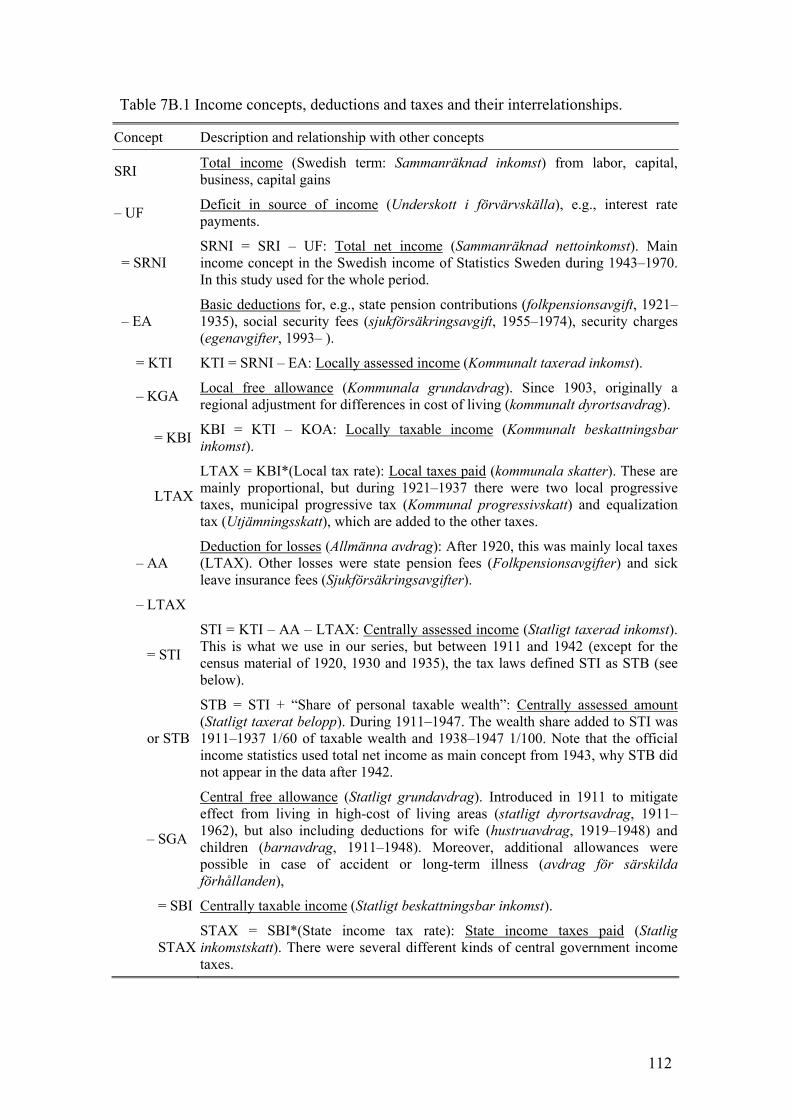
112

Table 7B.1 Income concepts, deductions and taxes and their interrelationships.

Concept Description and relationship with other concepts

SRI Total income (Swedish term: Sammanräknad inkomst) from labor, capital, business, capital gains

�– UF Deficit in source of income (Underskott i förvärvskälla), e.g., interest rate payments.

= SRNI SRNI = SRI �– UF: Total net income (Sammanräknad nettoinkomst). Main income concept in the Swedish income of Statistics Sweden during 1943�–1970. In this study used for the whole period.

�– EA Basic deductions for, e.g., state pension contributions (folkpensionsavgift, 1921�–1935), social security fees (sjukförsäkringsavgift, 1955�–1974), security charges (egenavgifter, 1993�– ).

= KTI KTI = SRNI �– EA: Locally assessed income (Kommunalt taxerad inkomst).

�– KGA Local free allowance (Kommunala grundavdrag). Since 1903, originally a regional adjustment for differences in cost of living (kommunalt dyrortsavdrag).

= KBI KBI = KTI �– KOA: Locally taxable income (Kommunalt beskattningsbar inkomst).

LTAX

LTAX = KBI*(Local tax rate): Local taxes paid (kommunala skatter). These are mainly proportional, but during 1921�–1937 there were two local progressive taxes, municipal progressive tax (Kommunal progressivskatt) and equalization tax (Utjämningsskatt), which are added to the other taxes.

�– AA Deduction for losses (Allmänna avdrag): After 1920, this was mainly local taxes (LTAX). Other losses were state pension fees (Folkpensionsavgifter) and sick leave insurance fees (Sjukförsäkringsavgifter).

�– LTAX

= STI

STI = KTI �– AA �– LTAX: Centrally assessed income (Statligt taxerad inkomst). This is what we use in our series, but between 1911 and 1942 (except for the census material of 1920, 1930 and 1935), the tax laws defined STI as STB (see below).

or STB

STB = STI + �“Share of personal taxable wealth�”: Centrally assessed amount(Statligt taxerat belopp). During 1911�–1947. The wealth share added to STI was 1911�–1937 1/60 of taxable wealth and 1938�–1947 1/100. Note that the official income statistics used total net income as main concept from 1943, why STB did not appear in the data after 1942.

�– SGA

Central free allowance (Statligt grundavdrag). Introduced in 1911 to mitigate effect from living in high-cost of living areas (statligt dyrortsavdrag, 1911�–1962), but also including deductions for wife (hustruavdrag, 1919�–1948) and children (barnavdrag, 1911�–1948). Moreover, additional allowances were possible in case of accident or long-term illness (avdrag för särskilda förhållanden),

= SBI Centrally taxable income (Statligt beskattningsbar inkomst).

STAX STAX = SBI*(State income tax rate): State income taxes paid (Statlig inkomstskatt). There were several different kinds of central government income taxes.

113

Table 7B.2 The four income sources used in the compositional analysis in Sweden,

1912�–2006.

Income source Description

Wages Includes wages and salaries and is basically defined in the same way both before and after 1991.

Capital income Includes interest earnings, dividends and real estate income. In the period before 1991, we add �“capital income�” (interests and dividends) and �“real estate income�” together.77 After 1991, estimate capital income from the �“new capital income�”, which includes both the old concept and capital gains. Hence, we break out interest earnings and dividends (called inkomst av ränta in the income statistics), private rental income (inkomst av uthyrning av privatbostad) and special rental income (inkomst av positiv räntefördelning).

Business income Includes mainly income from privately held firms. Before 1991, we add together �“entrepreneurial income�” and �“farm income�”. After 1991, we use �“business income�”.

Capital gains Includes net gains from sales of real estate and other assets.

77 Formally, one part of the real estate income was also included in business income after 1991, namely income from public rental buildings. However, this only concerned so-called �“physical persons�” (private individuals) and not �“judicial persons�” (public and private companies) which instead had to report all of their income (including that from real estate) as entrepreneurial income and which was the largest part of the two incomes. Leif Johansson at Statistics Sweden (from a discussion on June 15, 2005) also would believe that the absolute majority of the real estate income before 1991 should refer to what would after 1991 have been included in capital income. For these reasons, we place all of real estate income in the capital income in our long-run series.

114

Table 7C.1 Reference totals for tax units and income in Sweden, 1903-2006 Income excl. capital gains Income incl. capital gains Total Tax Share Total income Total income tax units returns (col. 2/1) Sum Ave. Sum Ave.

N N % (TSEK) (col. 4/1) (TSEK) (col. 8/1) Year (1) (2) (3) (4) (5) (8) (9) 1903 2,659,911 191,515 7.2 1,389,293 522 1,406,589 529 1904 2,687,207 1,441,809 537 1,459,759 543 1905 2,706,379 1,483,502 548 1,501,971 555 1906 2,727,842 1,601,276 587 1,621,211 594 1907 2,756,634 328,992 11.9 1,743,376 632 1,765,080 640 1908 2,784,634 1,782,905 640 1,805,101 648 1909 2,799,518 1,755,932 627 1,777,792 635 1910 2,830,113 1,943,329 687 1,967,523 695 1911 2,856,711 700,954 24.5 2,013,619 705 2,038,688 714 1912 2,888,302 741,919 25.7 2,100,446 727 2,126,596 736 1913 2,908,770 2,222,844 764 2,250,518 774 1914 2,941,668 2,310,515 785 2,339,280 795 1915 2,976,466 2,482,713 834 2,513,622 844 1916 3,011,266 1,010,963 33.6 2,940,643 977 2,977,253 989 1917 3,051,956 3,623,331 1,187 3,668,441 1,202 1918 3,104,099 5,044,212 1,625 5,107,011 1,645 1919 3,117,303 1,813,876 58.2 6,298,162 2,020 6,376,572 2,046 1920 3,146,313 2,024,462 64.3 7,547,072 2,399 7,641,031 2,429 1921 3,178,804 6,159,471 1,938 6,236,155 1,962 1922 3,217,520 5,177,282 1,609 5,241,738 1,629 1923 3,233,086 4,953,887 1,532 5,015,562 1,551 1924 3,277,477 4,958,474 1,513 5,020,205 1,532 1925 3,310,033 5,101,173 1,541 5,164,681 1,560 1926 3,344,617 5,237,633 1,566 5,302,840 1,585 1927 3,382,095 5,345,823 1,581 5,412,377 1,600 1928 3,411,417 5,420,466 1,589 5,487,949 1,609 1929 3,443,967 5,737,820 1,666 5,809,254 1,687 1930 3,471,440 2,100,000 60.5 5,900,304 1,700 5,973,761 1,721 1931 3,509,250 5,667,049 1,615 5,737,602 1,635 1932 3,540,812 5,395,869 1,524 5,463,046 1,543 1933 3,569,615 5,328,643 1,493 5,394,983 1,511 1934 3,596,654 2,213,000 61.5 5,725,887 1,592 5,797,172 1,612 1935 3,616,987 2,269,000 62.7 6,105,505 1,688 6,181,516 1,709 1936 3,659,455 6,327,644 1,729 6,406,421 1,751 1937 3,679,432 2,394,000 65.1 6,855,515 1,863 6,940,864 1,886 1938 3,691,394 7,255,456 1,966 7,345,784 1,990 1939 3,701,699 2,547,000 68.8 7,809,324 2,110 7,906,548 2,136 1940 3,712,732 2,637,000 71.0 8,512,235 2,293 8,618,210 2,321 1941 3,721,269 2,737,000 73.6 9,422,040 2,532 9,539,342 2,563 1942 3,713,351 10,520,534 2,833 10,651,511 2,868 1943 3,715,298 2,955,890 79.6 11,065,749 2,978 11,202,683 3,015 1944 3,720,658 3,003,973 80.7 11,709,195 3,147 11,854,193 3,186 1945 3,701,136 3,074,993 83.1 12,602,660 3,405 12,758,863 3,447

115

1946 3,727,199 3,131,168 84.0 14,591,812 3,915 14,753,058 3,958 1947 3,751,937 3,240,670 86.4 16,166,881 4,309 16,323,556 4,351 1948 3,770,950 3,367,806 89.3 18,014,723 4,777 18,165,108 4,817 1949 3,769,391 3,384,834 89.8 18,645,789 4,947 18,775,907 4,981 1950 3,777,033 3,401,393 90.1 19,563,440 5,180 19,673,224 5,209 1951 4,363,129 3,791,083 86.9 22,885,687 5,245 22,982,724 5,267 1952 4,413,809 3,721,611 84.3 26,577,977 6,022 26,690,383 6,047 1953 4,458,901 3,732,619 83.7 27,467,838 6,160 27,583,831 6,186 1954 4,514,116 3,795,327 84.1 29,242,354 6,478 29,365,586 6,505 1955 4,582,359 3,899,843 85.1 32,291,992 7,047 32,428,330 7,077 1956 4,644,564 3,934,072 84.7 34,888,533 7,512 35,035,633 7,543 1957 4,712,198 3,995,344 84.8 36,502,787 7,746 36,656,476 7,779 1958 4,789,073 4,029,342 84.1 38,167,789 7,970 38,328,210 8,003 1959 4,872,546 4,081,406 83.8 40,123,929 8,235 40,292,302 8,269 1960 4,959,080 4,190,155 84.5 44,245,603 8,922 44,430,805 8,959 1961 5,059,839 4,277,753 84.5 48,185,654 9,523 48,386,952 9,563 1962 5,152,249 4,229,111 82.1 53,165,500 10,319 53,387,066 10,362 1963 5,243,201 4,326,942 82.5 57,858,292 11,035 58,099,461 11,081 1964 5,341,505 4,431,848 83.0 63,604,263 11,908 63,868,889 11,957 1965 5,440,809 4,541,358 83.5 69,980,068 12,862 70,270,741 12,915 1966 5,529,968 4,579,902 82.8 76,798,500 13,888 77,117,129 13,945 1967 5,750,422 5,086,784 88.5 85,122,755 14,803 85,460,455 14,862 1968 5,876,561 5,148,562 87.6 90,676,471 15,430 91,003,771 15,486 1969 6,036,078 5,299,008 87.8 97,923,883 16,223 98,345,983 16,293 1970 6,194,967 5,441,976 87.8 108,654,568 17,539 109,060,268 17,605 1971 6,320,018 5,487,290 86.8 118,419,028 18,737 118,727,677 18,786 1972 6,333,098 5,377,931 84.9 128,282,502 20,256 128,660,770 20,316 1973 6,350,879 5,412,041 85.2 137,286,578 21,617 137,786,877 21,696 1974 6,464,266 5,574,282 86.2 157,524,389 24,368 158,216,541 24,476 1975 6,496,063 5,705,452 87.8 183,188,876 28,200 184,073,602 28,336 1976 6,526,143 5,826,869 89.3 207,853,848 31,849 208,966,808 32,020 1977 6,559,497 5,990,972 91.3 232,215,863 35,401 233,385,873 35,580 1978 6,592,278 6,372,054 96.7 259,385,859 39,347 260,946,683 39,584 1979 6,629,136 6,431,194 97.0 284,682,262 42,944 286,079,081 43,155 1980 6,670,790 6,494,749 97.4 318,496,317 47,745 319,844,679 47,947 1981 6,705,740 6,531,845 97.4 348,888,051 52,028 350,612,945 52,285 1982 6,740,072 6,565,341 97.4 377,085,887 55,947 379,852,901 56,357 1983 6,773,449 6,609,388 97.6 407,703,146 60,191 412,040,798 60,832 1984 6,803,684 6,657,145 97.8 445,966,952 65,548 449,501,558 66,067 1985 6,830,258 6,701,312 98.1 488,718,732 71,552 492,943,601 72,171 1986 6,856,978 6,742,286 98.3 529,142,905 77,169 534,778,674 77,990 1987 6,893,476 6,787,936 98.5 579,733,510 84,099 587,878,378 85,280 1988 6,936,033 6,826,256 98.4 630,089,899 90,843 647,227,486 93,314 1989 6,984,652 6,874,984 98.4 700,291,628 100,261 722,610,112 103,457 1990 7,030,954 6,923,689 98.5 784,428,517 111,568 805,695,957 114,593 1991 7,060,631 7,087,528 100.4 856,232,513 121,269 893,271,977 126,514 1992 7,081,441 7,107,925 100.4 880,700,744 124,367 895,409,092 126,444 1993 7,109,685 7,139,138 100.4 912,094,785 128,289 926,303,618 130,288 1994 7,144,570 7,178,295 100.5 951,108,791 133,123 983,645,820 137,677 1995 7,163,497 7,201,488 100.5 990,246,452 138,235 1,006,748,895 140,539 1996 7,177,410 7,217,214 100.6 1,034,366,816 144,114 1,071,513,690 149,290

116

1997 7,187,081 7,232,695 100.6 1,076,806,119 149,825 1,130,844,902 157,344 1998 7,200,331 7,248,321 100.7 1,126,508,147 156,452 1,186,654,380 164,806 1999 7,215,231 7,262,257 100.7 1,188,708,879 164,750 1,286,073,700 178,244 2000 7,239,597 7,287,016 100.7 1,253,659,417 173,167 1,378,939,984 190,472 2001 7,273,123 7,321,060 100.7 1,312,767,595 180,496 1,371,991,000 188,638 2002 7,311,797 7,362,419 100.7 1,362,756,329 186,378 1,403,278,014 191,920 2003 7,350,260 7,405,489 100.8 1,414,031,516 192,378 1,459,078,346 198,507 2004 7,395,545 7,454,633 100.8 1,458,857,002 197,262 1,517,305,205 205,165 2005 7,448,581 7,513,754 100.9 1,515,189,510 203,420 1,606,753,012 215,713 2006 7,525,396 7,595,286 100.9 1,588,210,209 211,047 1,714,402,902 227,816

Note 1: Total income has been adjusted so that it includes social benefits (unemployment insurance, sick-leave pay, etc which are taxable incomes after 1974) for the whole period. Note 2: Tax returns as share of total tax units exceeds 100% after 1990 since that year�’s tax reform led to non-resident Swedes to file taxes in case they had some capital income. Setting a cap at 100% has a negligible effect on the reported shares (about 0.4 percent).