Tools for Analysis of Dynamic Systems: Lyapunov s Methodszak/ECE680/Lyapunov_ECE_680.pdf · 6 Outline Notation using simple examples of dynamical system models Objective of analysis

1

Tools for Analysis of Dynamical Systems: Lyapunov’s Methods

Stan Żak

School of Electrical and Computer Engineering

ECE 680 Fall 2017

2

A. M. Lyapunov’s (1857--1918) Thesis

3

Lyapunov’s Thesis

4

Lyapunov’s Thesis Translated

5

Some Details About Translation

6

Outline Notation using simple examples of

dynamical system models Objective of analysis of a nonlinear

system Equilibrium points Lyapunov functions Stability

Barbalat’s lemma

7

A Spring-Mass Mechanical System

x---displacement of the mass from the rest position

8

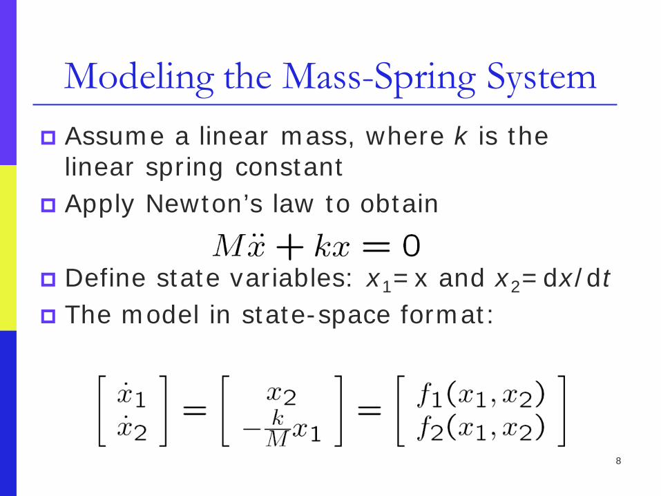
Modeling the Mass-Spring System Assume a linear mass, where k is the

linear spring constant Apply Newton’s law to obtain Define state variables: x1=x and x2=dx/dt The model in state-space format:

9

Analysis of the Spring-Mass System Model

The spring-mass system model is linear time-invariant (LTI)

Representing the LTI system in standard state-space format

10

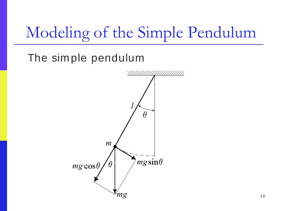
Modeling of the Simple Pendulum The simple pendulum

11

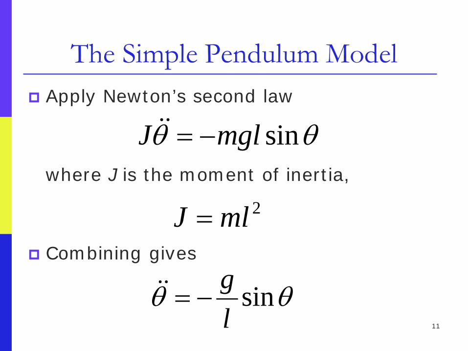
The Simple Pendulum Model Apply Newton’s second law

where J is the moment of inertia, Combining gives

θθ sinmglJ −=

2mlJ =

θθ sinlg

−=

12

State-Space Model of the Simple Pendulum

Represent the second-order differential equation as an equivalent system of two first-order differential equations

First define state variables, x1=θ and x2=dθ/dt Use the above to obtain state–space

model (nonlinear, time invariant)

13

Objectives of Analysis of Nonlinear Systems

Similar to the objectives pursued when investigating complex linear systems

Not interested in detailed solutions, rather one seeks to characterize the system behavior---equilibrium points and their stability properties

A device needed for nonlinear system analysis summarizing the system behavior, suppressing detail

14

Summarizing Function (D.G. Luenberger, 1979)

A function of the system state vector

As the system evolves in time, the summarizing function takes on various values conveying some information about the system

15

Summarizing Function as a First-Order Differential Equation

The behavior of the summarizing

function describes a first-order differential equation

Analysis of this first-order differential equation in some sense a summary analysis of the underlying system

16

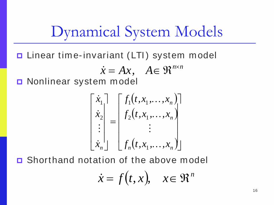
Dynamical System Models Linear time-invariant (LTI) system model

Nonlinear system model

Shorthand notation of the above model

nnA,Axx ×ℜ∈=

( ) nxxtfx ℜ∈= ,,

( )( )

( )

=

nn

n

n

n x,,x,tf

x,,x,tfx,,x,tf

x

xx

1

12

11

2

1

17

More Notation System model Solution

Example: LTI model, Solution of the LTI modeling equation

( ) ( )( ) ( ) 00 xtx,tx,tftx ==

( ) ( )00 x,t;txtx =

( ) 00 xx,Axx ==

( ) 0xetx At=

18

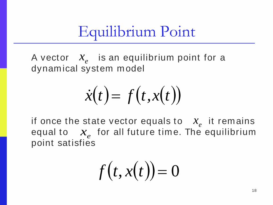
Equilibrium Point A vector is an equilibrium point for a

dynamical system model

if once the state vector equals to it remains

equal to for all future time. The equilibrium point satisfies

ex

( ) ( )( )tx,tftx =

exex

( )( ) 0, =txtf

19

Formal Definition of Equilibrium

A point xe is called an equilibrium point of dx/dt=f(t,x), or simply an equilibrium, at time t0 if for all t ≥ t0,

f(t, xe)=0 Note that if xe is an equilibrium

of our system at t0, then it is also an equilibrium for all τ ≥ t0

20

Equilibrium Points for LTI Systems

For the time invariant system dx/dt=f(x) a point is an equilibrium at some

time τ if and only if it is an equilibrium at all times

21

Equilibrium State for LTI Systems LTI model

Any equilibrium state must satisfy

If exist, then we have unique equilibrium state

( ) Axx,tfx ==

0=eAxex

1−A

0=ex

22

Equilibrium States of Nonlinear Systems

A nonlinear system may have a

number of equilibrium states

The origin, x=0, may or may not be an equilibrium state of a nonlinear system

23

Translating the Equilibrium of Interest to the Origin

If the origin is not the

equilibrium state, it is always possible to translate the origin of the coordinate system to that state

So, no loss of generality is lost in assuming that the origin is the equilibrium state of interest

24

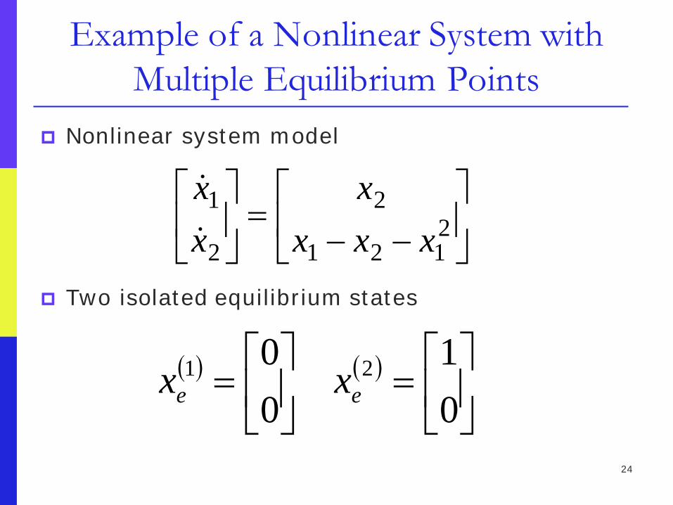
Example of a Nonlinear System with Multiple Equilibrium Points

Nonlinear system model

Two isolated equilibrium states

−−

=

2121

2

2

1

xxxx

xx

( ) ( )

=

=

01

00 21

ee xx

25

Isolated Equilibrium

An equilibrium point xe in Rn is an isolated equilibrium point if there is an r>0 such that the r-neighborhood of xe contains no equilibrium points other than xe

26

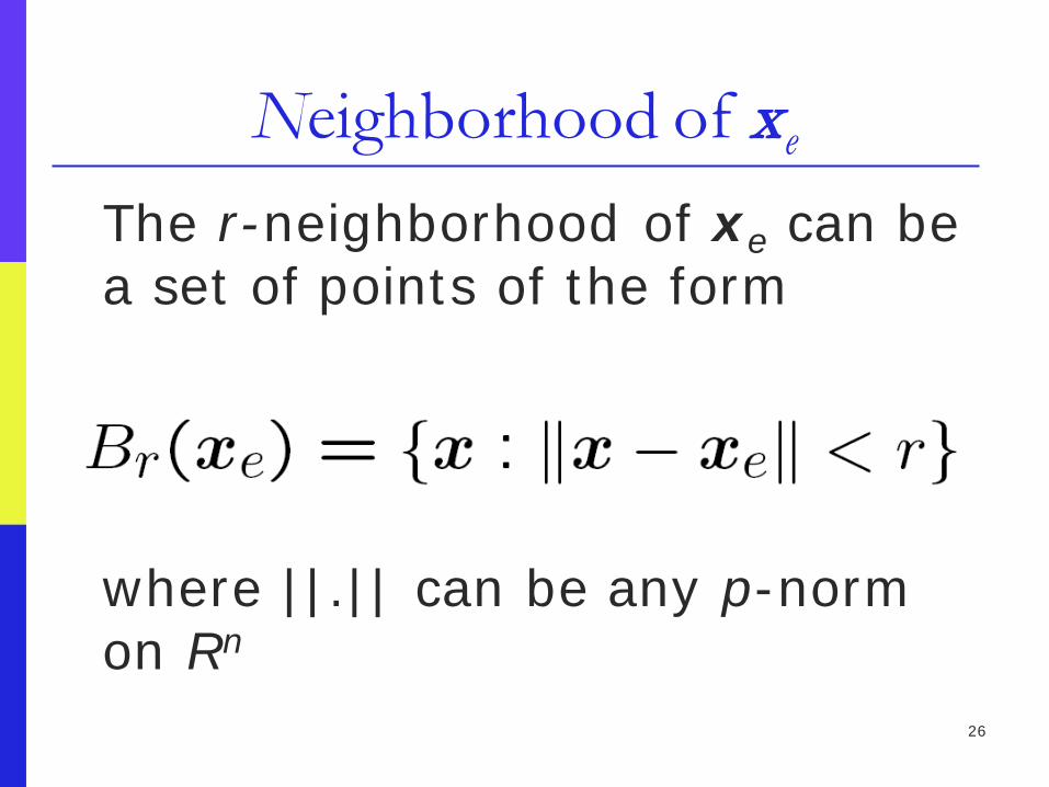
Neighborhood of xe

The r-neighborhood of xe can be a set of points of the form

where ||.|| can be any p-norm

on Rn

27

Remarks on Stability Stability properties characterize

the system behavior if its initial state is close but not at the equilibrium point of interest

When an initial state is close to the equilibrium pt., the state may remain close, or it may move away from the equilibrium point

28

An Informal Definition of Stability

An equilibrium state is stable if whenever the initial state is near that point, the state remains near it, perhaps even tending toward the equilibrium point as time increases

29

Stability Intuitive Interpretation

30

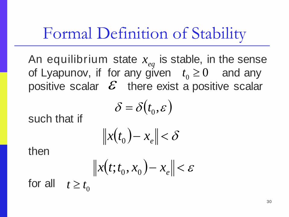
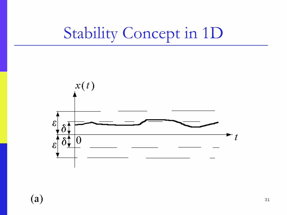
Formal Definition of Stability An equilibrium state is stable, in the sense

of Lyapunov, if for any given and any positive scalar there exist a positive scalar

such that if then for all

eqx0 0t ≥

ε( )εδδ ,0t=

( ) ε<− exxttx 00,;

( ) δ<− extx 0

0tt ≥

31

Stability Concept in 1D

32

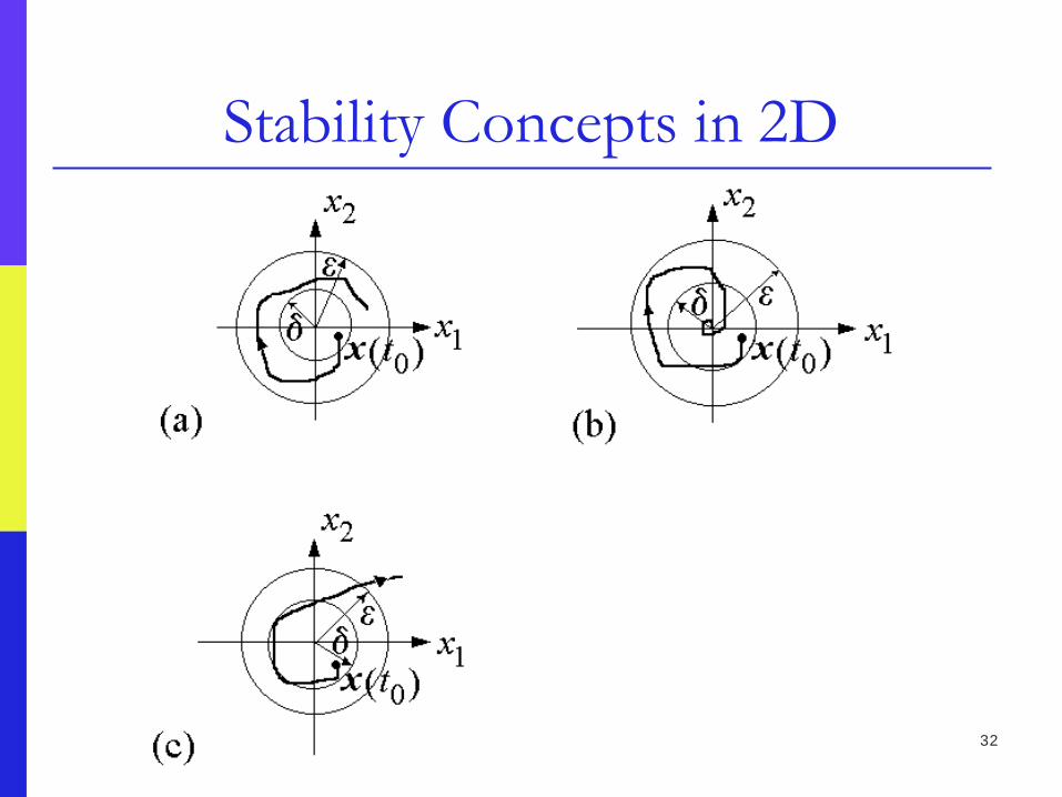
Stability Concepts in 2D

33

Further Discussion of Lyapunov Stability

Think of a contest between you,

the control system designer, and an adversary (nature?)---B. Friedland (ACSD, p. 43, Prentice-Hall, 1996)

34

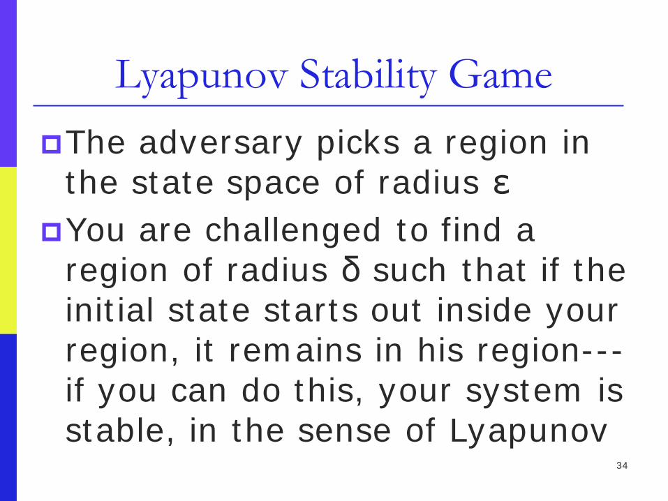
Lyapunov Stability Game The adversary picks a region in

the state space of radius ε You are challenged to find a

region of radius δ such that if the initial state starts out inside your region, it remains in his region---if you can do this, your system is stable, in the sense of Lyapunov

35

Lyapunov Stability---Is It Any Good?

Lyapunov stability is weak---it does not even imply that x(t) converges to xe as t approaches infinity

The states are only required to hover around the equilibrium state

The stability condition bounds the amount of wiggling room for x(t)

36

Asymptotic Stability i.s.L The property of an equilibrium

state of a differential equation that satisfies two conditions:

(stability) small perturbations in the initial condition produce small perturbations in the solution;

37

Second Condition for Asymptotic Stability of an Equilibrium

(attractivity of the equilibrium point) there is a domain of attraction such that whenever the initial condition belongs to this domain the solution approaches the equilibrium state at large times

38

Asymptotic Stability in the sense of Lyapunov (i.s.L.)

The equilibrium state is asymptotically stable if it is stable, and convergent, that is,

( ) ∞→→ tasxx,t;tx e00

39

Convergence Alone Does Not Guarantee Asymptotic Stability

Note: it is not sufficient that just

for asymptotic stability. We need

stability too! Why?

( ) ∞→→ tasxx,t;tx e00

40

How Long to the Equilibrium?

Asymptotic stability does not imply anything about how long it takes to converge to a prescribed neighborhood of xe

Exponential stability provides a way to express the rate of convergence

41

Asymptotic Stability of Linear Systems

An LTI system is asymptotically stable, meaning, the equilibrium state at the origin is asymptotically stable, if and only if the eigenvalues of A have negative real parts

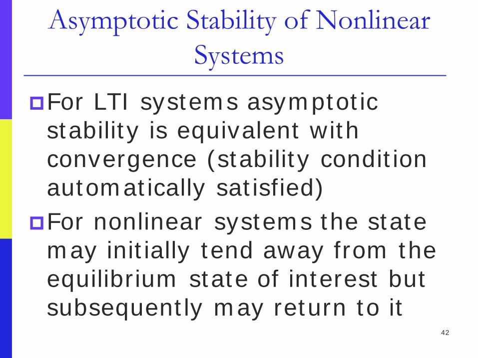
For LTI systems asymptotic stability is equivalent with convergence (stability condition automatically satisfied)

42

Asymptotic Stability of Nonlinear Systems

For LTI systems asymptotic stability is equivalent with convergence (stability condition automatically satisfied)

For nonlinear systems the state may initially tend away from the equilibrium state of interest but subsequently may return to it

43

Asymptotic Stability in 1D

44

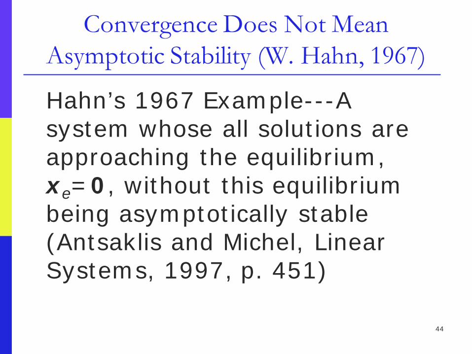
Convergence Does Not Mean Asymptotic Stability (W. Hahn, 1967)

Hahn’s 1967 Example---A system whose all solutions are approaching the equilibrium, xe=0, without this equilibrium being asymptotically stable (Antsaklis and Michel, Linear Systems, 1997, p. 451)

45

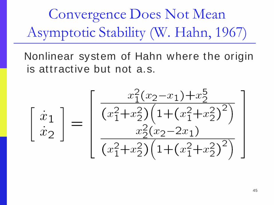
Convergence Does Not Mean Asymptotic Stability (W. Hahn, 1967)

Nonlinear system of Hahn where the origin is attractive but not a.s.

46

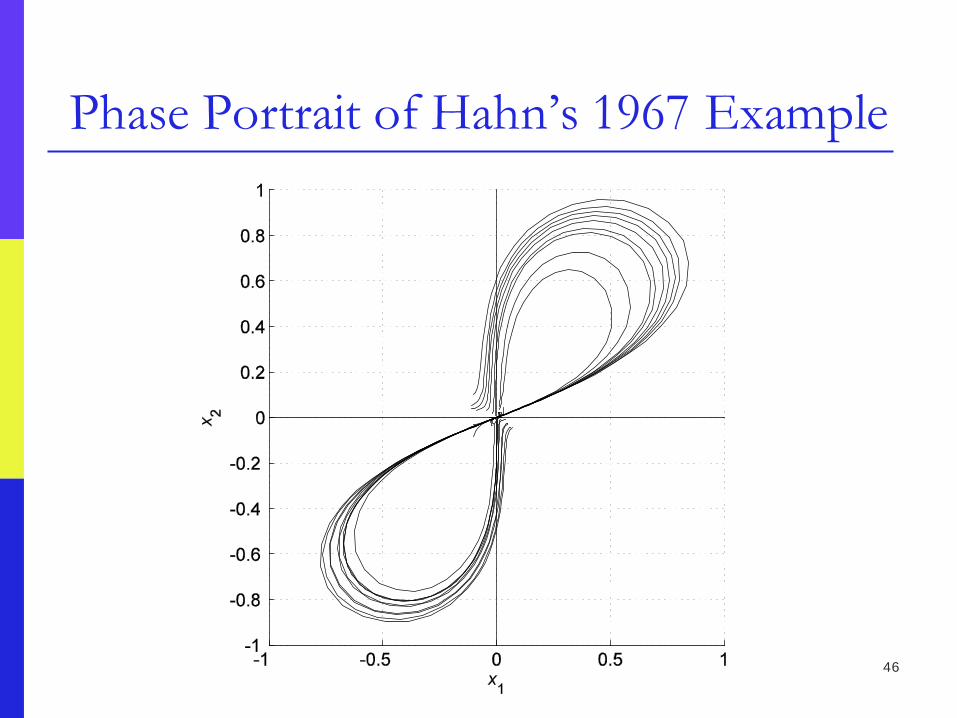
Phase Portrait of Hahn’s 1967 Example

47

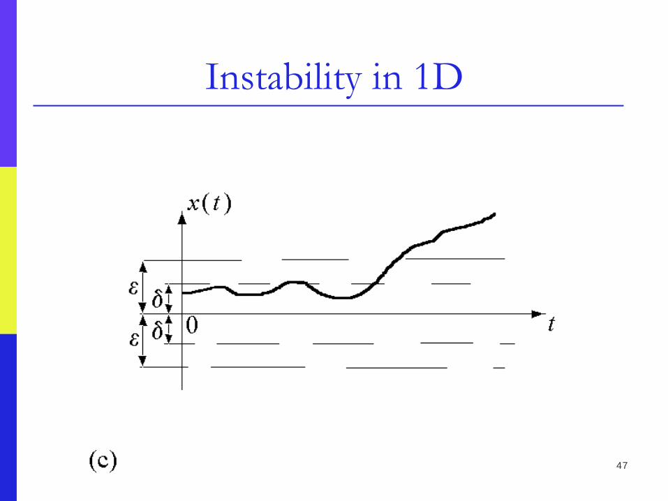
Instability in 1D

48

Lyapunov Functions---Basic Idea Seek an aggregate summarizing

function that continually decreases toward a minimum

For mechanical systems---energy of a free mechanical system with friction always decreases unless the system is at rest, equilibrium

49

Lyapunov Function Definition

A function that allows one to deduce stability is termed a Lyapunov function

50

Lyapunov Function Properties for Continuous Time Systems

Continuous-time system

Equilibrium state of interest

( ) ( )( )txftx =

ex

51

Three Properties of a Lyapunov Function

We seek an aggregate summarizing function V V is continuous V has a unique minimum with respect to all other points in some neighborhood of the equilibrium of interest

Along any trajectory of the system, the value of V never increases

52

Lyapunov Theorem for Continuous Systems

Continuous-time system

Equilibrium state of interest

( ) ( )( )txftx =

0=ex

53

Lyapunov Theorem---Negative Rate of Increase of V

If x(t) is a trajectory, then V(x(t)) represents the corresponding values of V along the trajectory

In order for V(x(t)) not to increase, we require

( )( ) 0≤txV

54

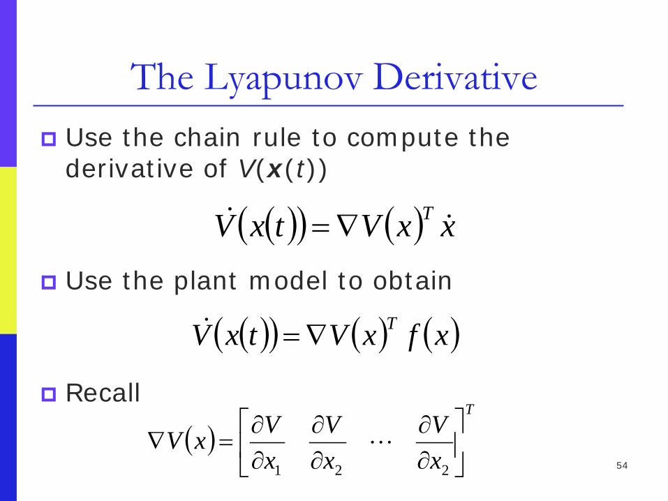
The Lyapunov Derivative Use the chain rule to compute the

derivative of V(x(t))

Use the plant model to obtain

Recall

( )( ) ( ) xxVtxV T ∇=

( )( ) ( ) ( )xfxVtxV T∇=

( )T

xV

xV

xVxV

∂∂

∂∂

∂∂

=∇221

55

Lyapunov Theorem for LTI Systems

The system dx/dt=Ax is

asymptotically stable, that is, the equilibrium state xe=0 is asymptotically stable (a.s), if and only if any solution converges to xe=0 as t tends to infinity for any initial x0

56

Lyapunov Theorem Interpretation

View the vector x(t) as defining

the coordinates of a point in an n-dimensional state space

In an a.s. system the point x(t)

converges to xe=0

57

Lyapunov Theorem for n=2

If a trajectory is converging to xe=0, it should be possible to find a nested set of closed curves V(x1,x2)=c, c≥0, such that decreasing values of c yield level curves shrinking in on the equilibrium state xe=0

58

Lyapunov Theorem and Level Curves

The limiting level curve

V(x1,x2)=V(0)=0 is 0 at the equilibrium state xe=0

The trajectory moves through the level curves by cutting them in the inward direction ultimately ending at xe=0

59

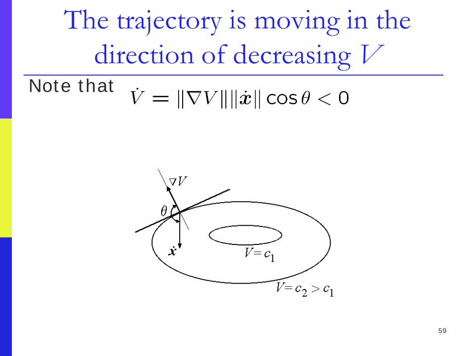
The trajectory is moving in the direction of decreasing V

Note that

60

Level Sets The level curves can be thought

of as contours of a cup-shaped surface

For an a.s. system, that is, for an a.s. equilibrium state xe=0, each trajectory falls to the bottom of the cup

61

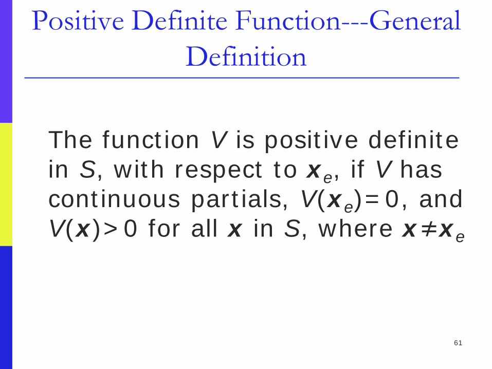
Positive Definite Function---General Definition

The function V is positive definite

in S, with respect to xe, if V has continuous partials, V(xe)=0, and V(x)>0 for all x in S, where x≠xe

62

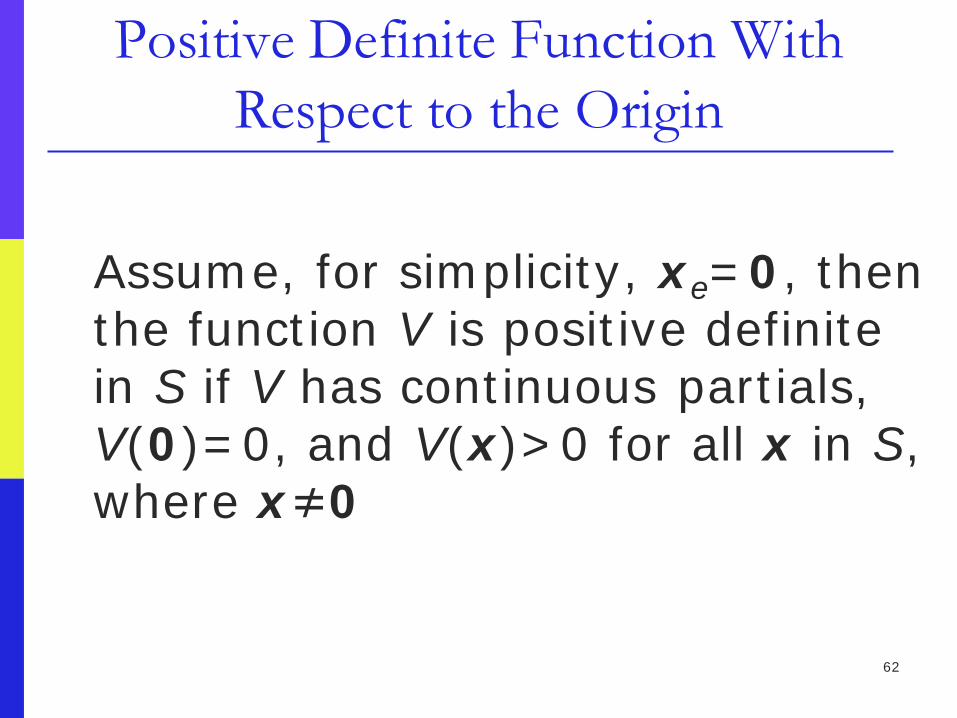
Positive Definite Function With Respect to the Origin

Assume, for simplicity, xe=0, then

the function V is positive definite in S if V has continuous partials, V(0)=0, and V(x)>0 for all x in S, where x≠0

63

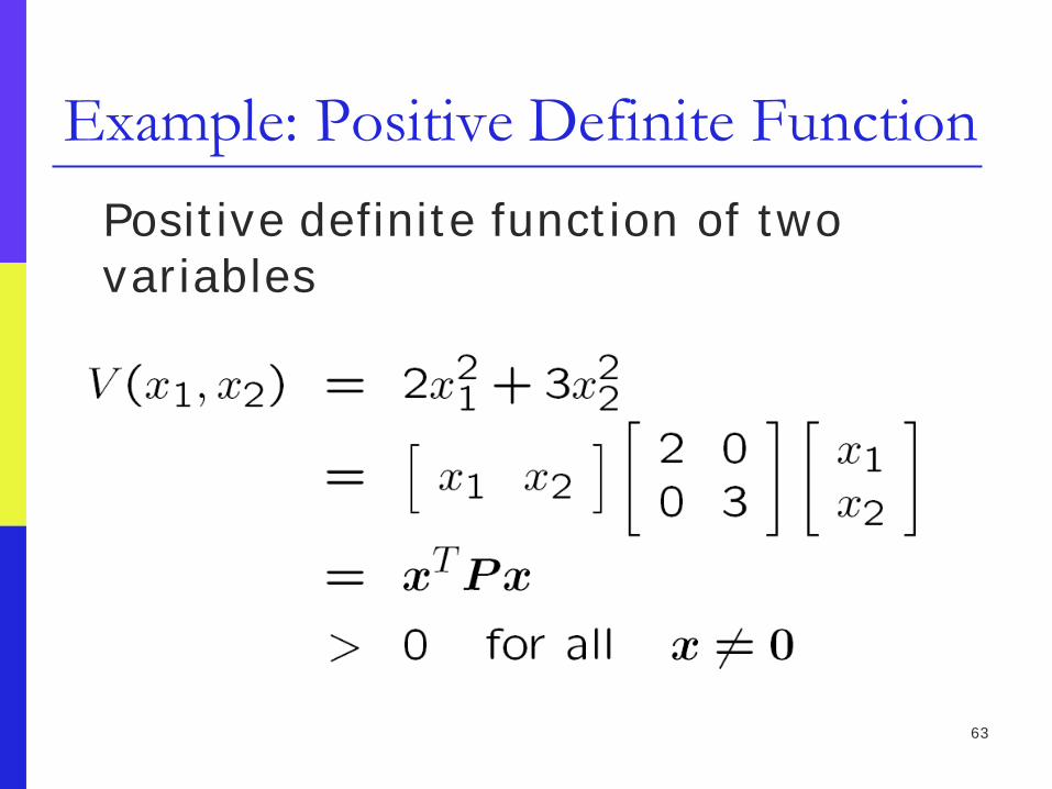
Example: Positive Definite Function Positive definite function of two

variables

64

Positive Semi-Definite Function---General Definition

The function V is positive semi-

definite in S, with respect to xe, if V has continuous partials, V(xe)=0, and V(x)≥0 for all x in S

65

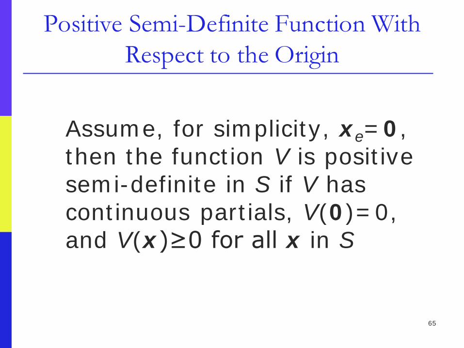
Positive Semi-Definite Function With Respect to the Origin

Assume, for simplicity, xe=0, then the function V is positive semi-definite in S if V has continuous partials, V(0)=0, and V(x)≥0 for all x in S

66

Example: Positive Semi-Definite Function

An example of positive semi-definite function of two variables

67

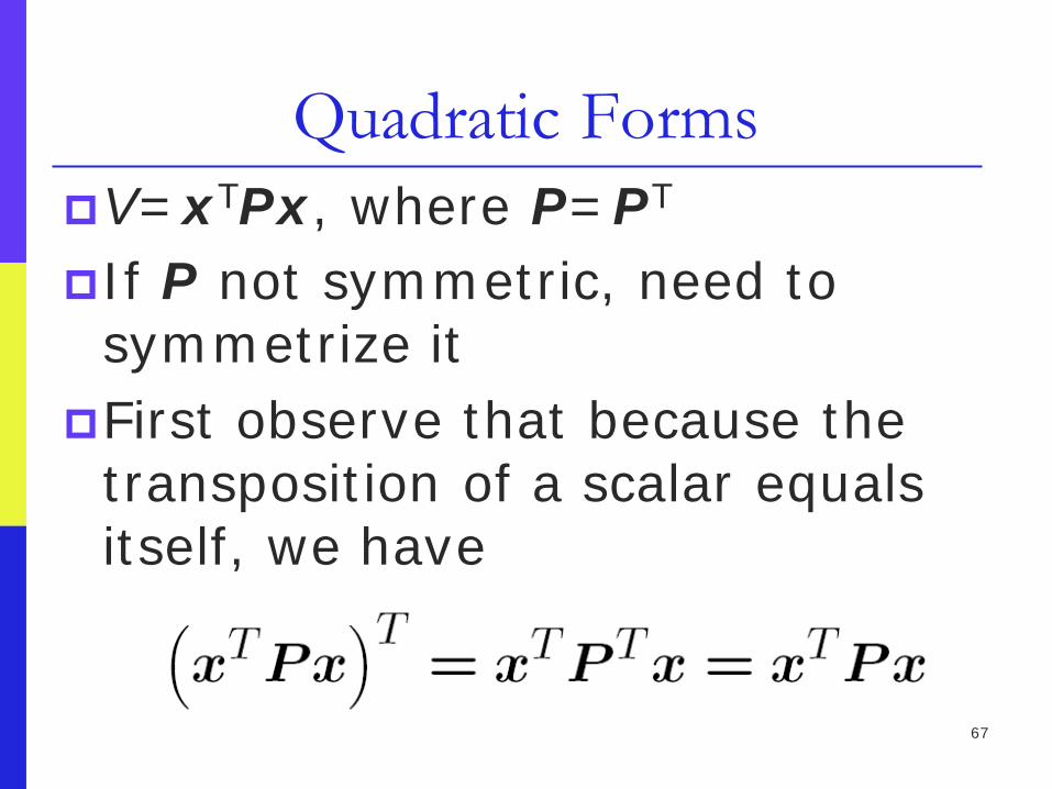
Quadratic Forms V=xTPx, where P=PT If P not symmetric, need to

symmetrize it First observe that because the

transposition of a scalar equals itself, we have

68

Symmetrizing Quadratic Form

Perform manipulations

Note that

69

Tests for Positive and Positive Semi-Definiteness of Quadratic Form

V=xTPx, where P=PT, is positive definite if and only if all eigenvalues of P are positive

V=xTPx, where P=PT, is positive semi-definite if and only if all eigenvalues of P are non-negative

70

Comments on the Eigenvalue Tests These tests are only good for the

case when P=PT. You must symmetrize P before applying the above tests

Other tests, the Sylvester’s criteria, involve checking the signs of principal minors of P

71

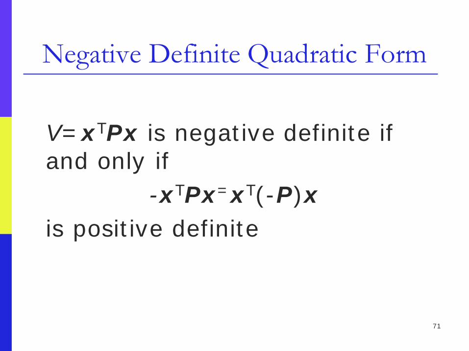
Negative Definite Quadratic Form

V=xTPx is negative definite if

and only if -xTPx=xT(-P)x

is positive definite

72

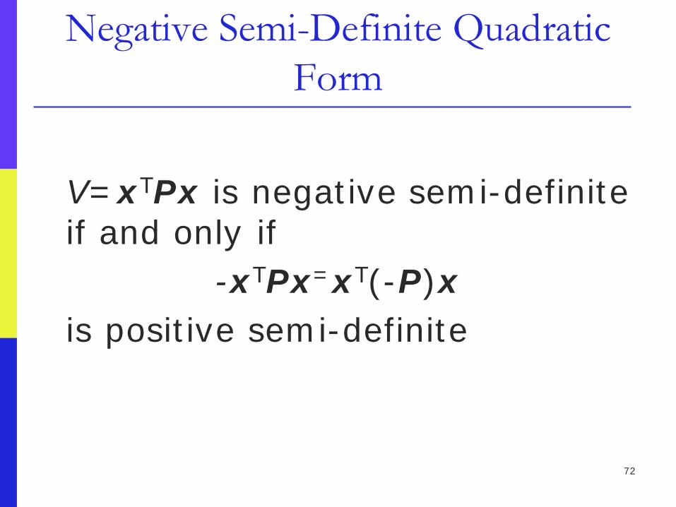
Negative Semi-Definite Quadratic Form

V=xTPx is negative semi-definite

if and only if -xTPx=xT(-P)x

is positive semi-definite

73

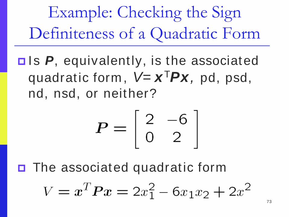
Example: Checking the Sign Definiteness of a Quadratic Form

Is P, equivalently, is the associated quadratic form, V=xTPx, pd, psd, nd, nsd, or neither?

The associated quadratic form

74

Example: Symmetrizing the Underlying Matrix of the Quadratic Form

Applying the eigenvalue test to the given quadratic form would seem to indicate that the quadratic form is pd, which turns out to be false

Need to symmetrize the underlying matrix first and then can apply the eigenvalue test

75

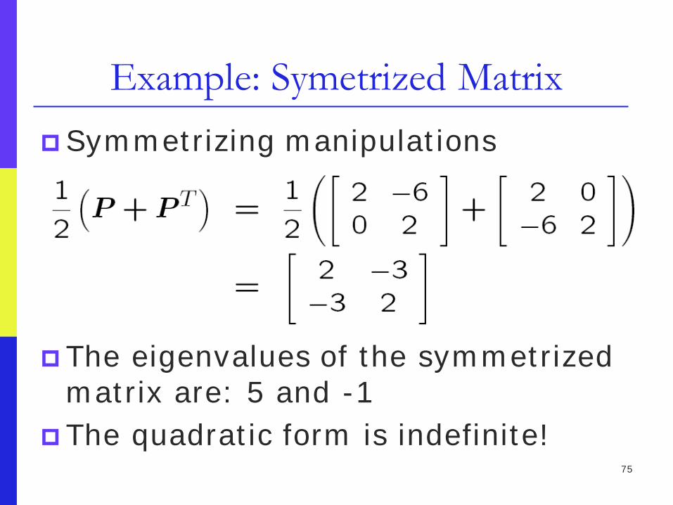
Example: Symetrized Matrix Symmetrizing manipulations

The eigenvalues of the symmetrized matrix are: 5 and -1

The quadratic form is indefinite!

76

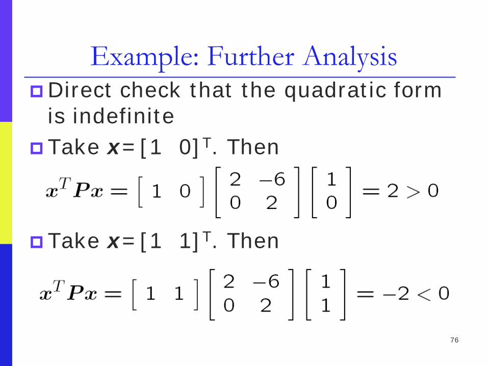
Example: Further Analysis Direct check that the quadratic form

is indefinite Take x=[1 0]T. Then Take x=[1 1]T. Then

77

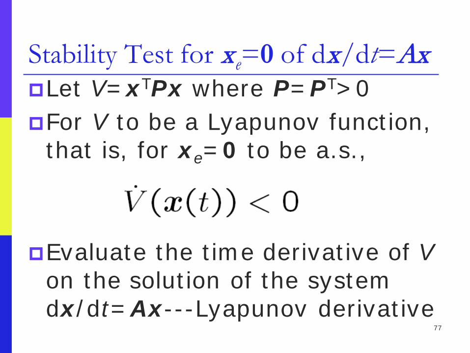
Stability Test for xe=0 of dx/dt=Ax Let V=xTPx where P=PT>0 For V to be a Lyapunov function,

that is, for xe=0 to be a.s., Evaluate the time derivative of V

on the solution of the system dx/dt=Ax---Lyapunov derivative

78

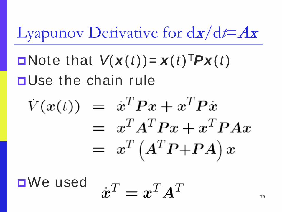
Lyapunov Derivative for dx/dt=Ax Note that V(x(t))=x(t)TPx(t) Use the chain rule

We used

79

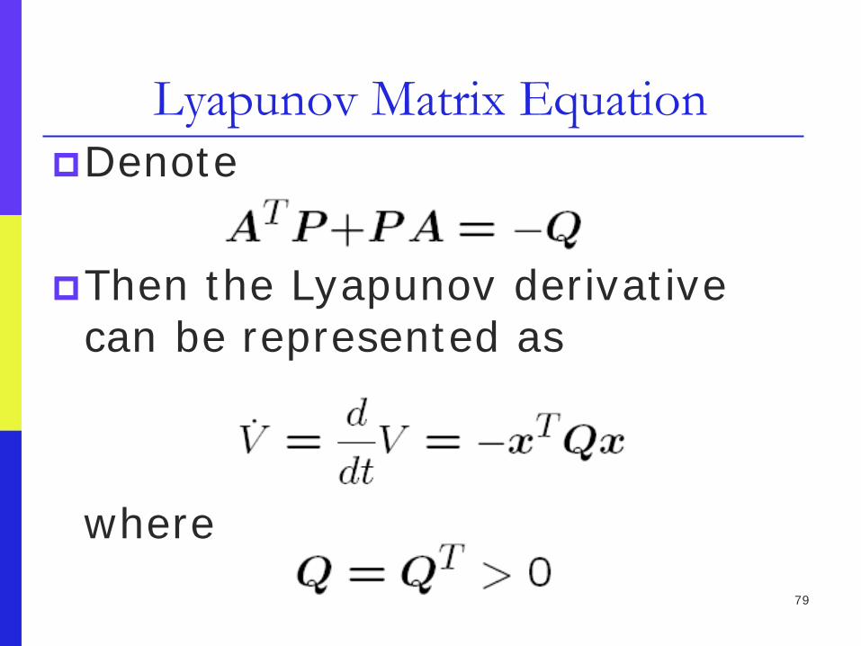
Lyapunov Matrix Equation Denote Then the Lyapunov derivative

can be represented as

where

80

Terms to Our Vocabulary Theorem---a major result of

independent interest Lemma---an auxiliary result that is

used as a stepping stone toward a theorem

Corollary---a direct consequence of a theorem, or even a lemma

81

Lyapunov Theorem The real matrix A is a.s., that is,

all eigenvalues of A have negative real parts if and only if for any the solution of the continuous matrix Lyapunov equation

is (symmetric) positive definite

82

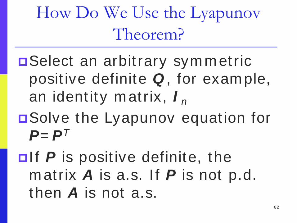
How Do We Use the Lyapunov Theorem?

Select an arbitrary symmetric positive definite Q , for example, an identity matrix, In

Solve the Lyapunov equation for P=PT

If P is positive definite, the matrix A is a.s. If P is not p.d. then A is not a.s.

83

How NOT to Use the Lyapunov Theorem

It would be no use choosing P to

be positive definite and then calculating Q

For unless Q turns out to be positive definite, nothing can be said about a.s. of A from the Lyapunov equation

84

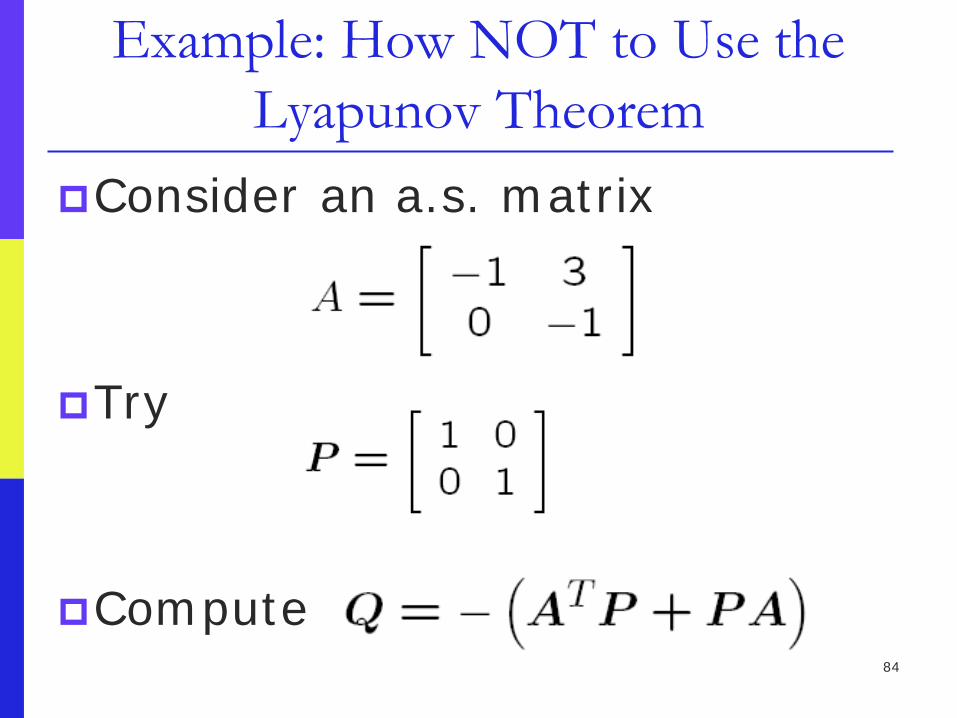
Example: How NOT to Use the Lyapunov Theorem

Consider an a.s. matrix

Try

Compute

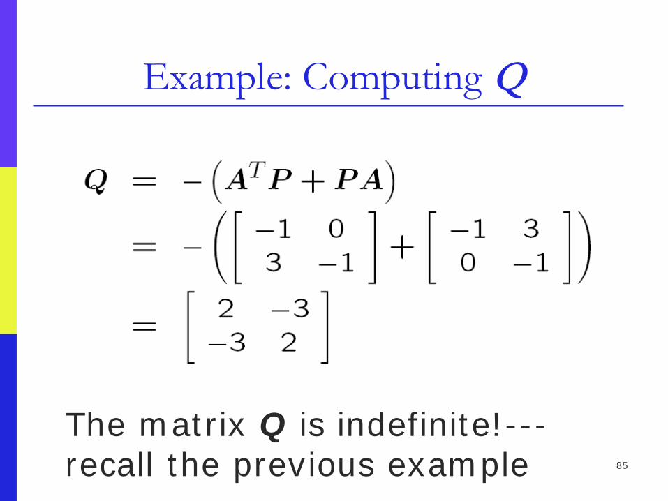
85

Example: Computing Q The matrix Q is indefinite!---

recall the previous example

86

Solving the Continuous Matrix Lyapunov Equation Using MATLAB

Use the MATLAB’s command lyap Example:

Q=I2

P=lyap(A’,Q) P=[0.50 0.75;0.75 2.75]

Eigenvalues of P are positive: 0.2729 and 2.9771; P is positive definite

87

Limitations of the Lyapunov Method

Usually, it is challenging to analyze the asymptotic stability of time-varying systems because it is very difficult to find Lyapunov functions with negative definite derivatives

When can one conclude asymptotic stability when the Lyapunov derivative is only negative semi-definite?

88

Some Properties of Time-Varying Functions

does not imply that f(t) has a limit as f(t) has a limit as does not imply that

89

More Properties of Time-Varying Functions

If f(t) is lower bounded and decreasing ( ), then it converges to a limit. (A well-known

result from calculus.)

But we do not know whether or not as

90

Preparation for Barbalat’s Lemma Under what conditions

We already know that the existence of the limit of f(t) as is not enough for

91

Continuous Function

A function f(t) is continuous if small changes in t result in small changes in f(t)

Intuitively, a continuous function is a function whose graph can be drawn without lifting the pencil from the paper

92

Continuity on an Interval Continuity is a local property of a

function—that is, a function f is continuous, or not, at a particular point

A function being continuous on an interval means only that it is continuous at each point of the interval

93

Uniform Continuity A function f(t) is uniformly

continuous if it is continuous and, in addition, the size of the changes in f(t) depends only on the size of the changes in t but not on t itself

The slope of an uniformly continuous function slope is bounded, that is,

is bounded Uniform continuity is a global

property of a function

94

Properties of Uniformly Continuous Function

Every uniformly continuous function is continuous, but the converse is not true

A function is uniformly continuous, or not, on an entire interval

A function may be continuous at each point of an interval without being uniformly continuous on the entire interval

95

Examples Uniformly continuous:

f(t) = sin(t) Note that the slope of the above

function is bounded Continuous, but not uniformly

continuous on positive real numbers: f(t) = 1/t

Note that as t approaches 0, the changes in f(t) grow beyond any bound

96

State of an a.s. System With Bounded Input is Bounded

Example of Slotine and Li, “Applied Nonlinear Control,” p. 124, Prentice Hall, 1991

Consider an a.s. stable LTI system with bounded input

The state x is bounded because u is

bounded and A is a.s.

97

Output of a.s. System With Bounded Input is Uniformly Continuous

Because x is bounded and u is bounded, is bounded

Derivative of the output equation is The time derivative of the output is

bounded Hence, y is uniformly continuous

98

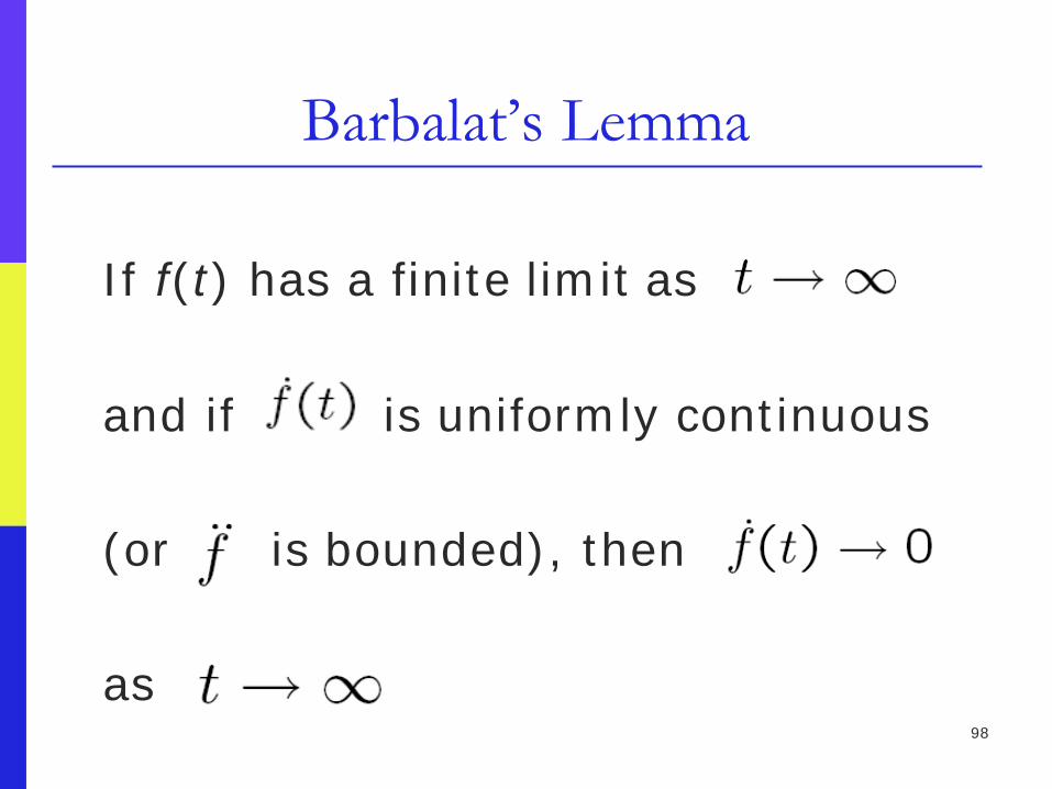
Barbalat’s Lemma If f(t) has a finite limit as and if is uniformly continuous (or is bounded), then as

99

Lyapunov-Like Lemma Given a real-valued function W(t,x)

such that W(t,x) is bounded below W(t,x) is negative semi-definite is uniformly continuous in t (or bounded) then

100

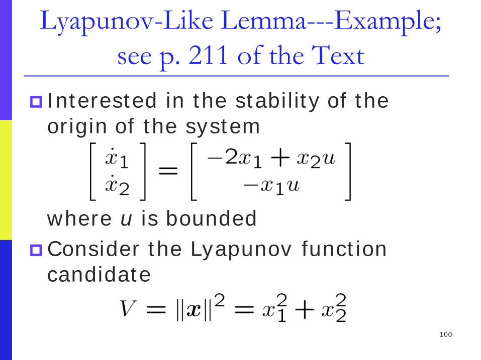
Lyapunov-Like Lemma---Example; see p. 211 of the Text

Interested in the stability of the origin of the system

where u is bounded Consider the Lyapunov function

candidate

101

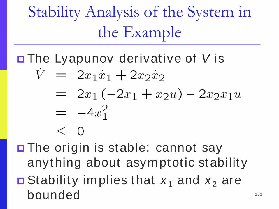
Stability Analysis of the System in the Example

The Lyapunov derivative of V is

The origin is stable; cannot say anything about asymptotic stability

Stability implies that x1 and x2 are bounded

102

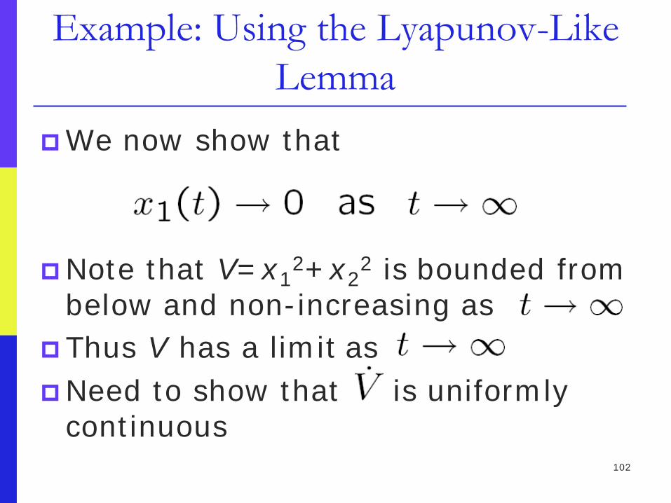
Example: Using the Lyapunov-Like Lemma

We now show that

Note that V=x12+x2

2 is bounded from below and non-increasing as

Thus V has a limit as Need to show that is uniformly

continuous

103

Example: Uniform Continuity of Compute the derivative of and

check if it is bounded

The function is uniformly continuous because is bounded Hence Therefore

104

Benefits of the Lyapunov Theory Solution to differential equation are

not needed to infer about stability properties of equilibrium state of interest

Barbalat’s lemma complements the Lyapunov Theorem

Lyapunov functions are useful in designing robust and adaptive controllers