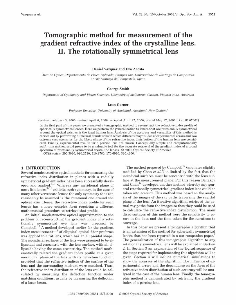
Tomographic method for measurement of the gradient refractive index of the crystalline lens. II. The rotationally symmetrical lens

1Srsommrolm

ptCiwTllempltcmo

Vazquez et al. Vol. 23, No. 10 /October 2006 /J. Opt. Soc. Am. A 2551

Tomographic method for measurement of thegradient refractive index of the crystalline lens.

II. The rotationally symmetrical lens

Daniel Vazquez and Eva Acosta

Area de Optica, Departamento de Fisica Aplicada, Campus Sur, Universidade de Santiago de Compostela,15782 Santiago de Compostela, Spain

George Smith

Department of Optometry and Vision Sciences, University of Melbourne, Carlton, Victoria 3053, Australia

Leon Garner

Professor Emeritus, University of Auckland, Auckland, New Zealand

Received February 3, 2006; revised April 6, 2006; accepted April 27, 2006; posted May 17, 2006 (Doc. ID 67662)

In the first part of this paper we presented a tomographic method to reconstruct the refractive index profile ofspherically symmetrical lenses. Here we perform the generalization to lenses that are rotationally symmetricalaround the optical axis, as is the ideal human lens. Analysis of the accuracy and versatility of this method iscarried out by performing numerical simulations in which different magnitudes of experimental errors and twoextreme case scenarios for the likely shape of the refractive index distribution of the human lens are consid-ered. Finally, experimental results for a porcine lens are shown. Conceptually simple and computationallyswift, this method could prove to be a valuable tool for the accurate retrieval of the gradient index of a broadspectrum of rotationally symmetrical crystalline lenses. © 2006 Optical Society of America

OCIS codes: 290.3030, 080.2710, 110.2760, 170.6960, 330.4300.

mifaetspttdrc

ilTr2tgsprlpi

. INTRODUCTIONeveral nondestructive optical methods for measuring theefractive index distribution in planes with a radiallyymmetrical gradient index have been successfully devel-ped and applied.1–8 Whereas any meridional plane ofost fish lenses9–11 exhibits such symmetry, in the case ofany other vertebrate lenses the only symmetry that can

easonably be assumed is the rotational one around theptical axis. Hence, the refractive index profile for suchenses has a more complex form requiring a different

athematical procedure to retrieve that profile.An initial nondestructive optical approximation to the

roblem of reconstructing the gradient index of a rota-ionally symmetrical eye lens was proposed byampbell.12 A method developed earlier for the gradient

ndex measurement1,13 of elliptical optical fiber preformsas applied to a rat lens, which has an ellipsoidal shape.he isoindicial surfaces of the lens were assumed to be el-

ipsoidal and concentric with the lens surface, with all el-ipsoids having the same eccentricity. The method math-matically related the gradient index profile at a giveneridional plane of the lens with its deflection function,

rovided that the refractive indices of the surface of theens and the surrounding medium were matched. Thus,he refractive index distribution of the lens could be cal-ulated by measuring the deflection function underatching conditions, usually by measuring the deflection

f a laser beam.

1084-7529/06/102551-15/$15.00 © 2

The method proposed by Campbell12 (and later slightlyodified by Chan et al.4) is limited by the fact that the

soindicial surfaces must be concentric with the lens sur-ace at the measurement plane. For this reason Beliakovnd Chan14 developed another method whereby any gen-ral rotationally symmetrical gradient index lens could beaken into account. This method was based on the analy-is of the images of the ray paths traversing the sagittallane of the lens. An iterative algorithm retrieved the ac-ual ray paths from the images so that they could be usedo calculate the refractive index distribution. The mainisadvantages of this method were the sensitivity to er-ors in the data and the time taken for the iterations toonverge.

In this paper we present a tomographic algorithm thats an extension of the method for spherically symmetricalenses that has been reported in a our companion paper.8

he generalization of this tomographic algorithm to anyotationally symmetrical lens will be explained in Section. In Section 3 an explanation of the logical sequence ofhe steps required for implementing this algorithm will beiven. Section 4 will include numerical simulations tohow the accuracy of the algorithm. The influence of ex-erimental errors and the dependence on the form of theefractive index distribution of such accuracy will be ana-yzed in the case of the human lens. Finally, the tomogra-hic method is demonstrated by retrieving the gradientndex of a porcine lens.

006 Optical Society of America

erHwarr

2Toaseg

tmlcwmssiio

crtiagtdearptWt

ibkg

B

Pf

at

E

w

dsr=aisc

rnpc

w

APcppspferws

Fda

2552 J. Opt. Soc. Am. A/Vol. 23, No. 10 /October 2006 Vazquez et al.

It is important to point out that we do not rule out thexistence of nonrotationally symmetrical features in theefractive index distribution of actual crystalline lenses.owever, because of their morphological characteristics15

e think that the most logical approach is to focus on thessumption of rotational symmetry. The retrieval of non-otational “perturbations” of this model is left as a furtherefinement of the tomographic method.

. THEORYhe theoretical bases we will turn to are similar to thosef the tomographic method explained in our first papernd applicable to spherical fish lenses.8 Thus, the empha-is will be on those features that are relevant to the gen-ralization of the method to any rotationally symmetricradient index lens.

The basic idea of the tomographic algorithm is to re-rieve the refractive index distribution from measure-ents of the optical paths of rays passing through the

ens. Although many different experimental techniquesan provide measurements of the optical path, here weill focus on the implementation of the tomographicethod with data obtained from laser ray tracing or laser

canning,4–6,8,12 given the conceptual and experimentalimplicity of this technique. We will show that by measur-ng the deflection produced by the lens for a collection ofncoming laser beams, the optical path covered by eachne of those rays can be calculated.

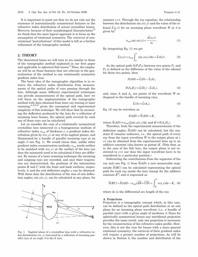
Let us consider the case of a rotationally symmetricalrystalline lens immersed in a homogeneous medium ofefractive index next of thickness t, a gradient index dis-ribution given by n�x ,z� at any of its sagittal planes, andlluminated by a bundle of parallel incoming rays at anngle � (see Fig. 1). We would stress that, unlike otherradient index reconstruction methods, next needs neithero be matched with n�x ,z� at the surface of the lens noroes the mismatch need to be calculated if they are differ-nt. By means of a laser scanning technique the incomingnd outgoing rays are recorded, and once their trajecto-ies are characterized, the positions of the intersectionoints B and C with the front and back surfaces, respec-ively, �, and the exit deflection angles � can be obtained.ith these data the distribution of the sine of exit deflec-

ion angles, sin ��x ,z�, can be calculated at any plane, for

ig. 1. Sagittal plane of a crystalline lens with a refractive in-ex distribution n�x ,z� traversed by a collection of incoming par-llel rays at an angle � to the Z axis.

nstance z= t. Through the ray equation, the relationshipetween the distribution sin ��x , t� and the value of the ei-onal L�x , t� for an incoming plane wavefront W at � isiven by8

next sin ��x,t� =�L�x,t�

�x. �1�

y integrating Eq. (1) we get

L�x,t� = next�0

x

sin ��x,t�dx + L�0,t�. �2�

As the optical path S�P1P2� between two points P1 and2 is defined as the difference of the value of the eikonal

or those two points, then

S�AD� = L�D� − L�A�,

S�AoDo� = L�Do� − L�Ao�, �3�

nd, since A and Ao are points of the wavefront W or-hogonal to the bundle of incoming rays,

L�A� = L�Ao�, �4�

q. (2) can be rewritten as

S�AD� = S�AD� + K, �5�

here S�AD��next�0xsin ��x , t�dx and K�S�AoDo�.

Therefore, from the experimental measurements of theeflection angles, S�AD� can be calculated, but the con-tant K remains unknown, i.e., the optical path of everyay from the input wavefront W to the output plane at zt can be obtained from the experimental data up to andditive constant (also known as piston) K. (Note that, asn the case of the fish lens, the output plane is not re-tricted to z= t nor does the input wavefront have to beonsidered in a particular position.)

Subtracting the contributions from the segments of theay and (see Fig. 1) from S�AD� a new measurable mag-itude S�BC� can be calculated representing the opticalath for each ray inside the lens (except for the additiveonstant K8) and is expressed as

S�BC� = S�AD� − next�AB + CD� =�B

C

n�x,z�ds − K, �6�

here ds is the differential arc length of the ray.

. Projectionsrojection is a tomographic concept which, in this case,an be defined as the optical path distribution at an exitlane for an incoming plane wavefront (i.e., a bundle ofarallel rays) with a given angle of incidence �. Since forpherically symmetrical lenses any meridional projectionrovides the same result, only one projection is necessaryor the reconstruction of the refractive index profile. How-ver, this is not the case for lenses with a more generalotational symmetry; the retrieval of their gradient indexill require a greater number of projections. As will be

hown in Section 4, the number and distribution of the

prfrw

arf

Ttrtp

BAi

w

a

Ww

iadnfm=dmtdbii

It

CTtlpiitTpraop

iClafattssweitbtBsdcitolrpwcgtgds

rdsbplvmswm

m

Vazquez et al. Vol. 23, No. 10 /October 2006 /J. Opt. Soc. Am. A 2553

rojections play a key role in the accuracy of the tomog-aphic reconstruction. Hence, optical path distributionsrom several projections must be considered in the tomog-aphic algorithm, requiring changes in its formulationith respect to the spherical case.Therefore, for a given projection at an angle � we haveset of N calculated values of S�BrCr�, a value for each

ay �r=1, . . . ,N�, and an unknown piston K related by theollowing formula

S�BrCr� = S�ArDr� − next�ArBr + CrDr� =�Br

Cr

n�x,z�dsr − K.

�7�

his set of values S�BrCr� for each projection constituteshe input data from which the tomographic algorithm willetrieve the refractive index distribution n�x ,z� and alsohe values of the constants K of each projection, as ex-lained in Ref. 8.

. Gradient Index Modelsgeneral model for a rotationally symmetrical refractive

ndex distribution around the optical axis Z is16–18:

n�r,z� = n0�z� + n1�z�r2 + n2�z�r4 + ¯ = �i=0

M

ni�z�r2i,

�8a�

here

ni�z� = �j=0

2�M−i�

nijzj �8b�

nd

r2 = x2 + y2. �8c�

ithout loss of generality and for the sake of simplicitye will perform all calculations at the plane Y=0.A slight variation of this model that we will also explore

s that of considering two halves of the crystalline lens,nterior and posterior, each with its own refractive indexistribution as described by Eq. (8a)–(8c), nant�x ,z� andpos�x ,z�, respectively. (Hereinafter this model will be re-

erred to as bipolynomial and the former as monopolyno-ial.) The union of both halves would take place at zzH, not necessarily the equatorial plane, where the con-itions of continuity of nant�x ,z� and npos�x ,z� are deter-ined by the layout of the crystalline fibers. Formed at

he equator of the lens and responsible for its gradient in-ex owing to cellular changes, these fibers extend towardoth the anterior and posterior poles of the lens. Thus, its very plausible and not restrictive to assume the follow-ng two conditions:

nant�x,zH� = npos�x,zH�,

�nant�x,zH�

�z=

�npos�x,zH�

�z. �9�

n this case, the tomographic algorithm will have to re-rieve not only the coefficients nant and npos, but also z .

. Ray Trajectories inside the Lenshe aim of the tomographic algorithm will be to retrieve

he values of the coefficients nij in the case of the monopo-ynomial model or nij

ant, nijpos, and zH in the case of the bi-

olynomial one. This is accomplished by inverting the linentegrals described in Eq. (7). Nevertheless, the refractivendex distribution n�x ,z� and the ray paths upon whichhose integrals occur are coupled by the ray equation.19

herefore, in the development of the proposed tomogra-hic algorithm we need to find approximations as accu-ate as possible to those ray paths. By doing so, n�x ,z�nd the ray paths can be uncoupled, making the problemf the tomographic inversion linear8 and minimizing com-utational effort.A first approximation, accurate for very weak gradient

ndices, is to consider straight paths joining points Br andr. However, although crystalline lenses do not show

arge variations in their refractive index,5,6,8,12,20,21 thispproximation may not be sufficiently accurate and someurther iterative procedure would be necessary to provideccurate results. For a weak gradient index (the case ofhe typical eye), the ray trajectories of the following itera-ions can be approximated by a short finite series oftraight line segments, for which the joining points of theegments are evaluated by ray-tracing algorithms22,23

ith the index distribution provided by the previous it-ration. Thus, an initial approximation of the ray pathsnside the lens as a straight line provides the first estima-ion of n�x ,z�, n0�x ,z�. With this initially calculated distri-ution and by using a ray-tracing algorithm, a point ofhe ray path is calculated at approximately BrCr /3 fromr by taking into account the incoming experimental

lope. Likewise, another point is calculated at the sameistance from Cr considering �r as an entry angle for thisalculation. By connecting Br with Cr through those twonterpolated points, each ray path is approximated byhree straight joined segments. Hence, a new estimationf the refractive index distribution n1�x ,z� can be calcu-ated and a further refinement of the ray trajectories car-ied out by assuming four instead of two intermediateoints. On this basis an iterative procedure is built forhich at each step the number of intermediate points in-

reases by two until the rms of the difference between theradient indices found at two consecutive iterations ei-her reaches a minimum, converges, or reaches a conver-ence tolerance that we set here as a value that is one or-er of magnitude lower than the retrieval accuracyought.

Provided that each iteration leads to a more accurateay approximation, this procedure allows crystalline gra-ient indices of different strengths to be measured. Thetronger the gradient, i.e., the higher the values reachedy the first partial derivatives, the more intermediateoints are needed to retrieve an accurate result and theonger it will take for the tomographic algorithm to con-erge. As we will see later, this convergence time is neverore than a few minutes for a modern desktop computer,

ince the incremental steps of the numerical ray-tracinge propose to use do not need to be too small for the to-ographic algorithm to provide good results.Thus, considering the monopolynomial gradient indexodel proposed at Eq. (8a)–(8c) and the expression given

acl

wtf

fl(��mCw

ieTSioSoccolnss

Tidtd

i

Fpt

2554 J. Opt. Soc. Am. A/Vol. 23, No. 10 /October 2006 Vazquez et al.

t Eq. (7) for S�BrCr�, the values of the expansion coeffi-ients nij and the pistons K for each projection are calcu-ated at each iteration by minimizing

�p=1

P

�r=1

Np ���i=0

M

�j=0

2�M−i�

nijfijprQ − Kp − S�BprCpr�2

, �10�

here P represents the total number of projections, Nphe number of rays per projection, Q the iteration (Q=0or the first iteration), and

fijprQ = ��Bpr

Q

CprQ

x2izjdlQ if Q = 0

�q=0

Q−1�Bpr

Q

Bprq+1

x2izjdlq +�Bpr

Q

CprQ

x2izjdlQ + �q�=0

Q−1 �Cpr

q�

Cprq�+1

x2izjdlq� if Q � 0� . �11�

pptc

nbBaeott�ctlshwSud

bnofcbio

ijprQ represents the line integrals over the 2Q+1 interpo-ated segments approaching the ray trajectories. In Eq.11) Bpr

q denotes the qth interpolated point from Bpr �Bpr0

Bpr�, Cprq� the q�th interpolated point from Cpr �Cpr

0

Cpr�, and dlq, dlQ, and dlq� the line elements for the seg-ents joining Bpr

q and Bprq+1, Bpr

Q and CprQ , and Cpr

q� and

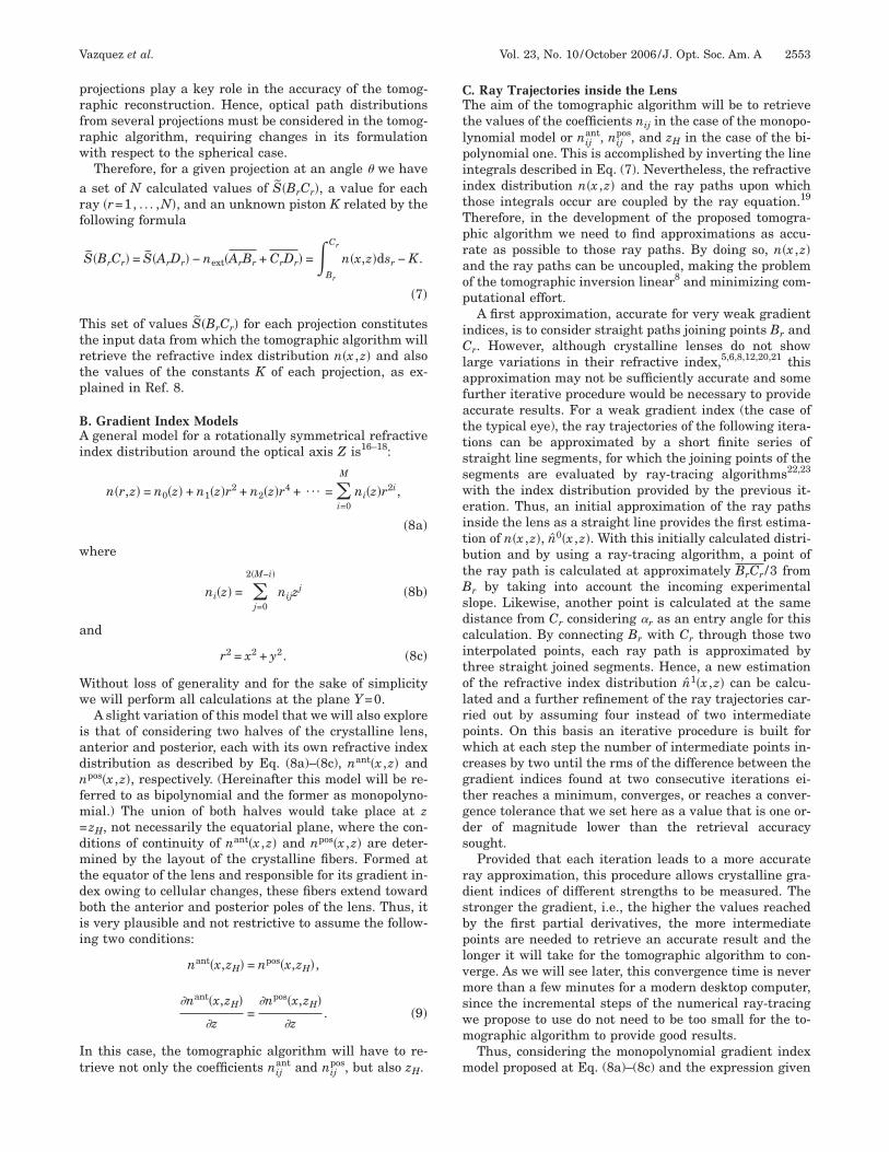
prq�+1, respectively. In order to explain this last expressione will now consider the case for Q=1.Having obtained a refractive index distribution n0�x ,z�

n the iteration Q=0, two points must be interpolated forach ray, one from Bpr and another from Cpr (see Fig. 2).o do this we propose to use the numerical ray-tracing ofharma et al.23 because of its accuracy for relatively large

ncremental steps, although it must be stressed that anyther ray-tracing algorithm could be used. Since theharma et al. algorithm does not make use of spatial co-rdinates we need to assume some approximations to cal-ulate the joining points of the interpolated segments. Byonsidering, for instance, an approximate average indexf n=1.4 for the case of the human lens5,20 and taking theength BprCpr from Bpr to Cpr, the incremental step of theumerical ray tracing23 for Q=1, where each segmenthould cover about one third of the complete ray path, iset as

�� =BprCpr/3

n=

BprCpr

4.2. �12�

hus, once the points Bpr1 and Cpr

1 are calculated, Eq. (10)s minimized in order to retrieve a new refractive indexistribution, n1�x ,z�, where in this case the line differen-ials of the integrations in Eq. (11) are dlq=1, dlQ=1, andlq�=1 (see Fig. 2).Therefore, if the Sharma et al. algorithm is used for an

teration Q the incremental step is set as

�� =BprCpr/�2Q + 1�

n, �13�

aying special attention to avoid the crossing of the rayropagation from Bpr and Cpr since, as explained above,he Sharma et al. algorithm does not make use of spatialoordinates.

Once the former iterative procedure retrieves a mo-opolynomial gradient index n�x ,z�, this distribution cane used to assess the quality of the result in optical terms.y using a ray-tracing algorithm and the experimental �pnd Bpr, rays are propagated through the retrieved gradi-nt index n�x ,z� to obtain the corresponding distributionsf the optical paths Sp�x , t� at plane z= t. Once they are seto zero at x=0, the differences between those distribu-ions and the experimentally retrieved Sp�x , t�, namelySp�x , t�, are calculated. Such differences show us how ac-urately n�x ,z� reproduces the aberrations and other op-ical properties of the lens. Thus, if those differences areower than or approximately equal to the error in mea-urement of Sp�x , t�, the tomographic algorithm could bealted at this point. If the differences are larger than orithin the same order of magnitude as the error in

˜p�x , t�, the result of the monopolynomial retrieval can besed to start a second phase in which a bipolynomial gra-ient index is considered.From n�x ,z� an initial estimation of the plane z=zH can

e obtained by calculating the position z� �0, t� for whichˆ �0,z� reaches a global maximum (which is why a previ-us monopolynomial retrieval is needed). Hence, theormer iterative procedure is applied to a bipolynomial re-onstruction of the gradient index. The only changes wille those of Eqs. (10) and (11) to take into account the ex-stence of two refractive index distributions at both sidesf z with their own coefficients nant and npos and the con-

ig. 2. Interpolation of two points, Bpr1 and Cpr

1 , in the iterativerocedure to obtain a trajectory (dashed curve) approximated tohe actual ray path (solid curve) from B to C .

H ij ij

tSmtd

3TNgpinrcp

AT3

lpa

ca

(

ctp

oriumitgc

etut

oaetrswtetA

l�

BIpptt(

at

tttfa

oPrndtsa

Fl

Vazquez et al. Vol. 23, No. 10 /October 2006 /J. Opt. Soc. Am. A 2555

inuity conditions given by Eq. (9). Likewise, if theharma et al. algorithm is used, the length of the incre-ental steps �� must be adjusted to ensure that half of

he interpolated points fall within each half of the lens, asivided by zH.

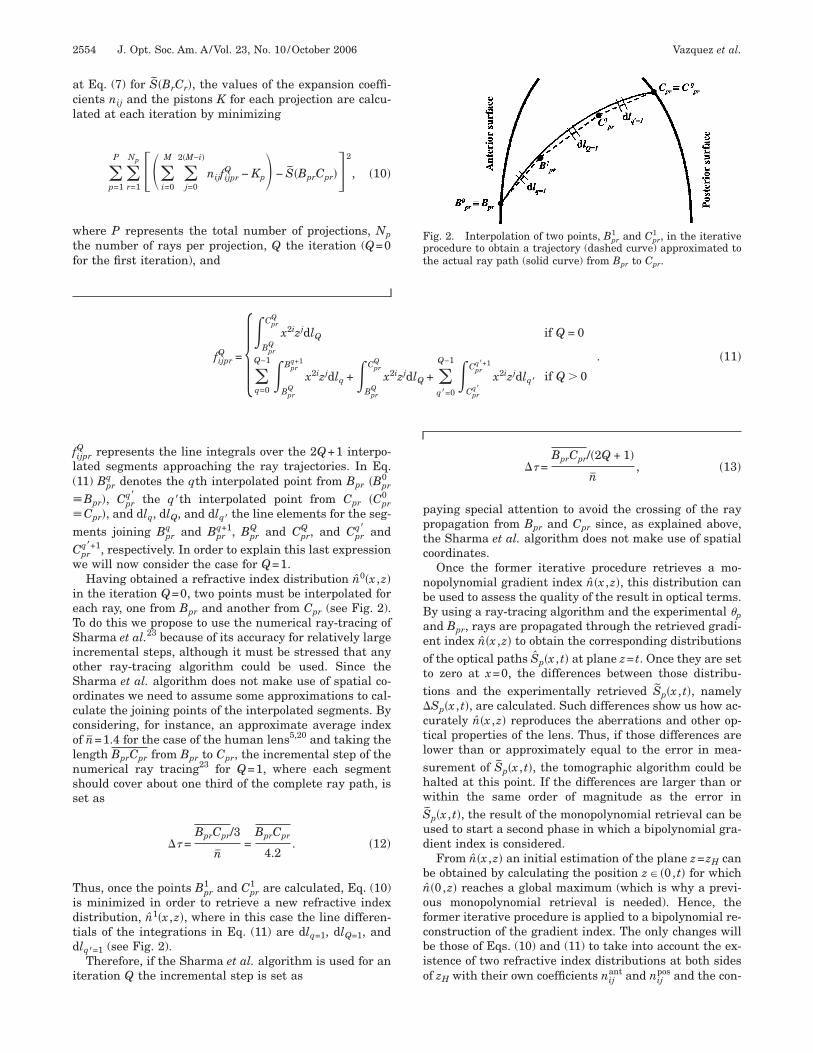
. LOGICAL SEQUENCE OF THEOMOGRAPHIC ALGORITHMext, each of the steps that make up the tomographic al-orithm and its logical sequence are explained in order torovide a better understanding of how the algorithm ismplemented. In Subsections 3.A and 3.B, the monopoly-omial and then the bipolynomial gradient index (GRIN)econstructions are considered, respectively, using flowharts to support a detailed explanation of the tomogra-hic procedure in each case.

. Monopolynomial Modelhe following items explain steps in the flow chart of Fig.:

1. INPUT DATA—These are the data provided by theaser scanning technique for P projections and Np rayser projection: �p, Bpr, Cpr, and sin �pr�x , t� (p=1, . . . ,Pnd r=1, . . . ,Np).2. PROCESS 1—Calculation of the optical paths ex-

ept for Kp: By using the laser scanning data and Eqs. (5)nd (7), the set of values S�BprCpr� is calculated.3. PROCESS 2—Monopolynomial GRIN retrieval

commencement of the iterative procedure): With the cal-

ig. 3. Flow chart of the tomographic algorithm for the monopo-ynomial reconstruction of the gradient index.

ulated values S�BprCpr� Eq. (10) is minimized to retrievehe nij coefficients and the pistons Kp, assuming 2Q inter-olated points [see Eq. (11)].4. PROCESS 3—GRIN check: This calculates the rms

f the difference between the refractive index distributionetrieved at the current iteration, nQ�x ,z� and the preced-ng one, nQ−1�x ,z� and compares it with the previous val-es of the rms. If the evolution of this magnitude does noteet any of the conditions set in Subsection 2.C, another

teration Q=Q+1 starts by performing PROCESS 4. Inhis case, the algorithm ends the iterative procedure andoes on to PROCESS 5. For the first two iterations, thisheck is inactive.

5. PROCESS 4—Point interpolation: the core of the it-rative procedure, making use of the Sharma et al. ray-racing algorithm to interpolate 2Q points for each ray bysing the refractive index distribution previously re-rieved and incremental steps as expressed in Eq. (13).

6. PROCESS 5—Numerical ray tracing: to obtain theptical differences �Sp�x , t� from which we can infer howccurately the retrieved function n�x ,z� reproduces thexperimental optical data and decide whether to refinehe result with a bipolynomial reconstruction. For thiseason the incremental step of this ray tracing must bemall enough to reproduce the optical behavior of the lensith an accuracy higher than the experimental errors in

he measurement of the optical path distribution at thexit of the lens. Likewise a rough estimate of the error inhe retrieval of n�x ,z�, �n, can be calculated (see Appendix).7. OUTPUT DATA—Consist of the retrieved monopo-

ynomial gradient index n�x ,z�, the optical differencesSp�x , t�, and a qualitative estimate of �n.

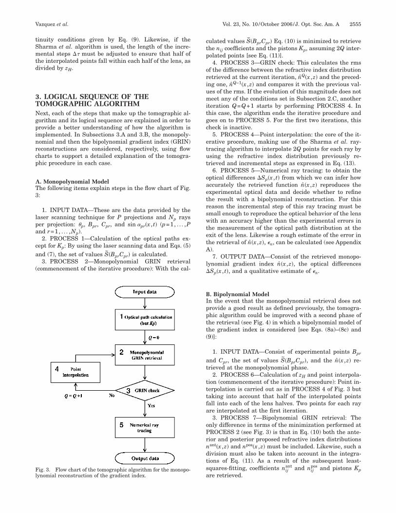
. Bipolynomial Modeln the event that the monopolynomial retrieval does notrovide a good result as defined previously, the tomogra-hic algorithm could be improved with a second phase ofhe retrieval (see Fig. 4) in which a bipolynomial model ofhe gradient index is considered [see Eqs. (8a)–(8c) and9)]:

1. INPUT DATA—Consist of experimental points Bpr

nd Cpr, the set of values S�BprCpr�, and the n�x ,z� re-rieved at the monopolynomial phase.

2. PROCESS 6—Calculation of zH and point interpola-ion (commencement of the iterative procedure): Point in-erpolation is carried out as in PROCESS 4 of Fig. 3 butaking into account that half of the interpolated pointsall into each of the lens halves. Two points for each rayre interpolated at the first iteration.3. PROCESS 7—Bipolynomial GRIN retrieval: The

nly difference in terms of the minimization performed atROCESS 2 (see Fig. 3) is that in Eq. (10) both the ante-ior and posterior proposed refractive index distributionsant�x ,z� and npos�x ,z� must be included. Likewise, such aivision must also be taken into account in the integra-ions of Eq. (11). As a result of the subsequent least-quares-fitting, coefficients nij

ant and nijpos and pistons Kp

re retrieved.

m

maq

iiMTmfisF

4AAelescdfwttro

l

1eda=oabtcoa

m

naide

rthmsdtgral

Fn

F(rp(

2556 J. Opt. Soc. Am. A/Vol. 23, No. 10 /October 2006 Vazquez et al.

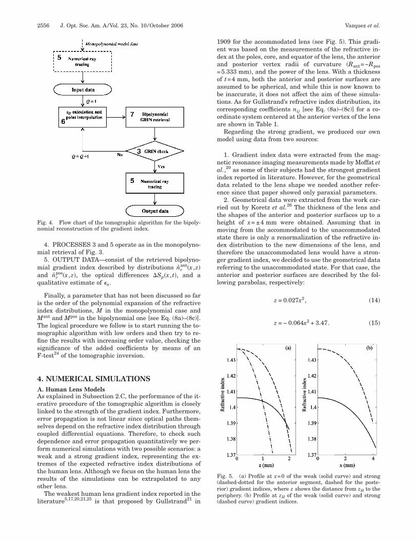
4. PROCESSES 3 and 5 operate as in the monopolyno-ial retrieval of Fig. 3.5. OUTPUT DATA—consist of the retrieved bipolyno-ial gradient index described by distributions nr

ant�x ,z�nd nr

pos�x ,z�, the optical differences �Sp�x , t�, and aualitative estimate of �n.

Finally, a parameter that has not been discussed so fars the order of the polynomial expansion of the refractivendex distributions, M in the monopolynomial case and

ant and Mpos in the bipolynomial one [see Eq. (8a)–(8c)].he logical procedure we follow is to start running the to-ographic algorithm with low orders and then try to re-

ne the results with increasing order value, checking theignificance of the added coefficients by means of an-test24 of the tomographic inversion.

. NUMERICAL SIMULATIONS. Human Lens Modelss explained in Subsection 2.C, the performance of the it-rative procedure of the tomographic algorithm is closelyinked to the strength of the gradient index. Furthermore,rror propagation is not linear since optical paths them-elves depend on the refractive index distribution throughoupled differential equations. Therefore, to check suchependence and error propagation quantitatively we per-orm numerical simulations with two possible scenarios: aeak and a strong gradient index, representing the ex-

remes of the expected refractive index distributions ofhe human lens. Although we focus on the human lens theesults of the simulations can be extrapolated to anyther lens.

The weakest human lens gradient index reported in theiterature5,17,20,21,25 is that proposed by Gullstrand21 in

ig. 4. Flow chart of the tomographic algorithm for the bipoly-omial reconstruction of the gradient index.

909 for the accommodated lens (see Fig. 5). This gradi-nt was based on the measurements of the refractive in-ex at the poles, core, and equator of the lens, the anteriornd posterior vertex radii of curvature �Rant=−Rpos5.333 mm�, and the power of the lens. With a thicknessf t=4 mm, both the anterior and posterior surfaces aressumed to be spherical, and while this is now known toe inaccurate, it does not affect the aim of these simula-ions. As for Gullstrand’s refractive index distribution, itsorresponding coefficients nij [see Eq. (8a)–(8c)] for a co-rdinate system centered at the anterior vertex of the lensre shown in Table 1.Regarding the strong gradient, we produced our ownodel using data from two sources:

1. Gradient index data were extracted from the mag-etic resonance imaging measurements made by Moffat etl.,20 as some of their subjects had the strongest gradientndex reported in literature. However, for the geometricalata related to the lens shape we needed another refer-nce since that paper showed only paraxial parameters.

2. Geometrical data were extracted from the work car-ied out by Koretz et al.26 The thickness of the lens andhe shapes of the anterior and posterior surfaces up to aeight of x= ±4 mm were obtained. Assuming that inoving from the accommodated to the unaccommodated

tate there is only a renormalization of the refractive in-ex distribution to the new dimensions of the lens, andherefore the unaccommodated lens would have a stron-er gradient index, we decided to use the geometrical dataeferring to the unaccommodated state. For that case, thenterior and posterior surfaces are described by the fol-owing parabolas, respectively:

z = 0.027x2, �14�

z = − 0.064x2 + 3.47. �15�

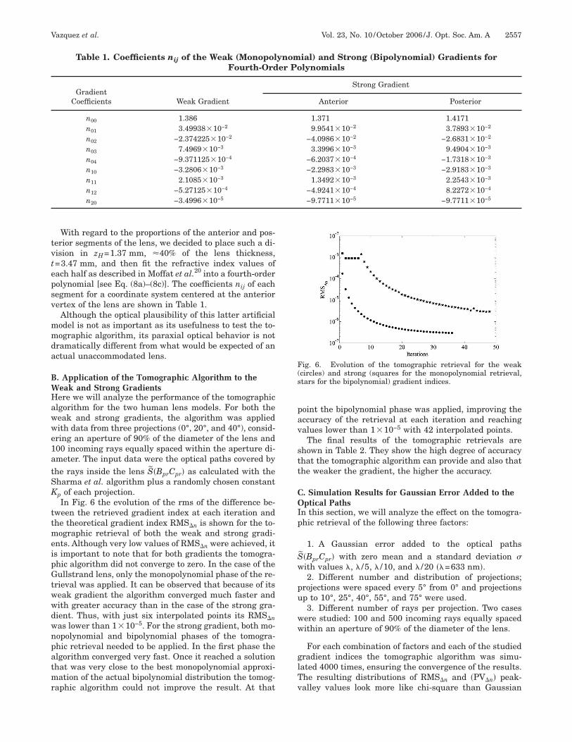
ig. 5. (a) Profile at x=0 of the weak (solid curve) and strongdashed-dotted for the anterior segment, dashed for the poste-ior) gradient indices, where z shows the distance from zH to theeriphery. (b) Profile at zH of the weak (solid curve) and strongdashed curve) gradient indices.

tvtepsv

mmda

BWHawwe1atSK

ttmeipGtwwdwnpatmr

pav

stt

COIp

Sw

pu

ww

glTv

F(s

Vazquez et al. Vol. 23, No. 10 /October 2006 /J. Opt. Soc. Am. A 2557

With regard to the proportions of the anterior and pos-erior segments of the lens, we decided to place such a di-ision in zH=1.37 mm, 40% of the lens thickness,=3.47 mm, and then fit the refractive index values ofach half as described in Moffat et al.20 into a fourth-orderolynomial [see Eq. (8a)–(8c)]. The coefficients nij of eachegment for a coordinate system centered at the anteriorertex of the lens are shown in Table 1.

Although the optical plausibility of this latter artificialodel is not as important as its usefulness to test the to-ographic algorithm, its paraxial optical behavior is not

ramatically different from what would be expected of anctual unaccommodated lens.

. Application of the Tomographic Algorithm to theeak and Strong Gradientsere we will analyze the performance of the tomographiclgorithm for the two human lens models. For both theeak and strong gradients, the algorithm was appliedith data from three projections (0°, 20°, and 40°), consid-ring an aperture of 90% of the diameter of the lens and00 incoming rays equally spaced within the aperture di-meter. The input data were the optical paths covered byhe rays inside the lens S�BprCpr� as calculated with theharma et al. algorithm plus a randomly chosen constantp of each projection.In Fig. 6 the evolution of the rms of the difference be-

ween the retrieved gradient index at each iteration andhe theoretical gradient index RMS�n is shown for the to-ographic retrieval of both the weak and strong gradi-

nts. Although very low values of RMS�n were achieved, its important to note that for both gradients the tomogra-hic algorithm did not converge to zero. In the case of theullstrand lens, only the monopolynomial phase of the re-

rieval was applied. It can be observed that because of itseak gradient the algorithm converged much faster andith greater accuracy than in the case of the strong gra-ient. Thus, with just six interpolated points its RMS�nas lower than 1�10−5. For the strong gradient, both mo-opolynomial and bipolynomial phases of the tomogra-hic retrieval needed to be applied. In the first phase thelgorithm converged very fast. Once it reached a solutionhat was very close to the best monopolynomial approxi-ation of the actual bipolynomial distribution the tomog-

aphic algorithm could not improve the result. At that

Table 1. Coefficients nij of the Weak (MonopolFourth-Ord

GradientCoefficients Weak Gradient

n00 1.386n01 3.49938�10−2

n02 −2.374225�10−2

n03 7.4969�10−3

n04 −9.371125�10−4

n10 −3.2806�10−3

n11 2.1085�10−3

n12 −5.27125�10−4

n20 −3.4996�10−5

oint the bipolynomial phase was applied, improving theccuracy of the retrieval at each iteration and reachingalues lower than 1�10−5 with 42 interpolated points.

The final results of the tomographic retrievals arehown in Table 2. They show the high degree of accuracyhat the tomographic algorithm can provide and also thathe weaker the gradient, the higher the accuracy.

. Simulation Results for Gaussian Error Added to theptical Paths

n this section, we will analyze the effect on the tomogra-hic retrieval of the following three factors:

1. A Gaussian error added to the optical paths˜ �BprCpr� with zero mean and a standard deviation �

ith values , /5, /10, and /20 �=633 nm�.2. Different number and distribution of projections;

rojections were spaced every 5° from 0° and projectionsp to 10°, 25°, 40°, 55°, and 75° were used.3. Different number of rays per projection. Two cases

ere studied: 100 and 500 incoming rays equally spacedithin an aperture of 90% of the diameter of the lens.

For each combination of factors and each of the studiedradient indices the tomographic algorithm was simu-ated 4000 times, ensuring the convergence of the results.he resulting distributions of RMS�n and �PV�n� peak-alley values look more like chi-square than Gaussian

ial) and Strong (Bipolynomial) Gradients forlynomials

Strong Gradient

Anterior Posterior

1.371 1.41719.9541�10−2 3.7893�10−2

−4.0986�10−2 −2.6831�10−2

3.3996�10−3 9.4904�10−3

−6.2037�10−4 −1.7318�10−3

−2.2983�10−3 −2.9183�10−3

1.3492�10−3 2.2543�10−3

−4.9241�10−4 8.2272�10−4

−9.7711�10−5 −9.7711�10−5

ig. 6. Evolution of the tomographic retrieval for the weakcircles) and strong (squares for the monopolynomial retrieval,tars for the bipolynomial) gradient indices.

ynomer Po

dstiaatl

c

end

chmr

W

S

Fviwaoc

F(i

2558 J. Opt. Soc. Am. A/Vol. 23, No. 10 /October 2006 Vazquez et al.

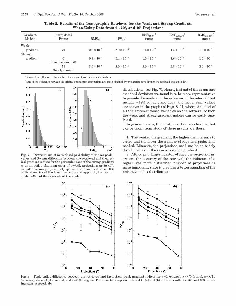
istributions (see Fig. 7). Hence, instead of the mean andtandard deviation we found it to be more representativeo provide the mode and the extremes of the interval thatnclude �68% of the cases about the mode. Such valuesre shown in the graphs of Figs. 8–11, where the effect ofll the aforementioned variables on the retrieval of bothhe weak and strong gradient indices can be easily ana-yzed.

In general terms, the most important conclusions thatan be taken from study of these graphs are these:

1. The weaker the gradient, the higher the tolerance torrors and the lower the number of rays and projectionseeded. Likewise, the projections need not be as widelyistributed as in the case of a strong gradient.2. Although a larger number of rays per projection in-

reases the accuracy of the retrieval, the influence of aigher and more distributed number of projections isore important, since it provides a better sampling of the

efractive index distribution.

al for the Weak and Strong Gradients°, and 40° Projections

na

RMS�S�0°�b

(mm)RMS�S�20°�

b

(mm)RMS�S�40°�

b

(mm)

10−6 1.4�10−7 1.4�10−7 1.9�10−7

10−3 1.6�10−3 1.6�10−3 1.6�10−3

10−5 2.9�10−6 2.8�10−6 2.2�10−6

by propagating rays through the retrieved gradient index.

weak gradient indices for �= (circles), �= /5 (stars), �= /10esent L and U. (a) and (b) are the results for 500 and 100 incom-

Table 2. Results of the Tomographic RetrievWhen Using Data from 0°, 20

GradientModels

InterpolatedPoints RMS�n PV�

eakgradient 70 2.9�10−7 2.0�

tronggradient 6

(monopolynomial)8.9�10−4 2.4�

74(bipolynomial)

3.2�10−6 2.9�

aPeak–valley difference between the retrieved and theoretical gradient indices.bRms of the difference between the original optical path distributions and those obtained

ig. 7. Distributions of normalized probability of the (a) peak–alley and (b) rms difference between the retrieved and theoret-cal gradient indices for the particular case of the strong gradientith an added Gaussian error of �= /5, projections up to 40°,nd 500 incoming rays equally spaced within an aperture of 90%f the diameter of the lens. Lower (L) and upper (U) bounds in-lude 68% of the cases about the mode.

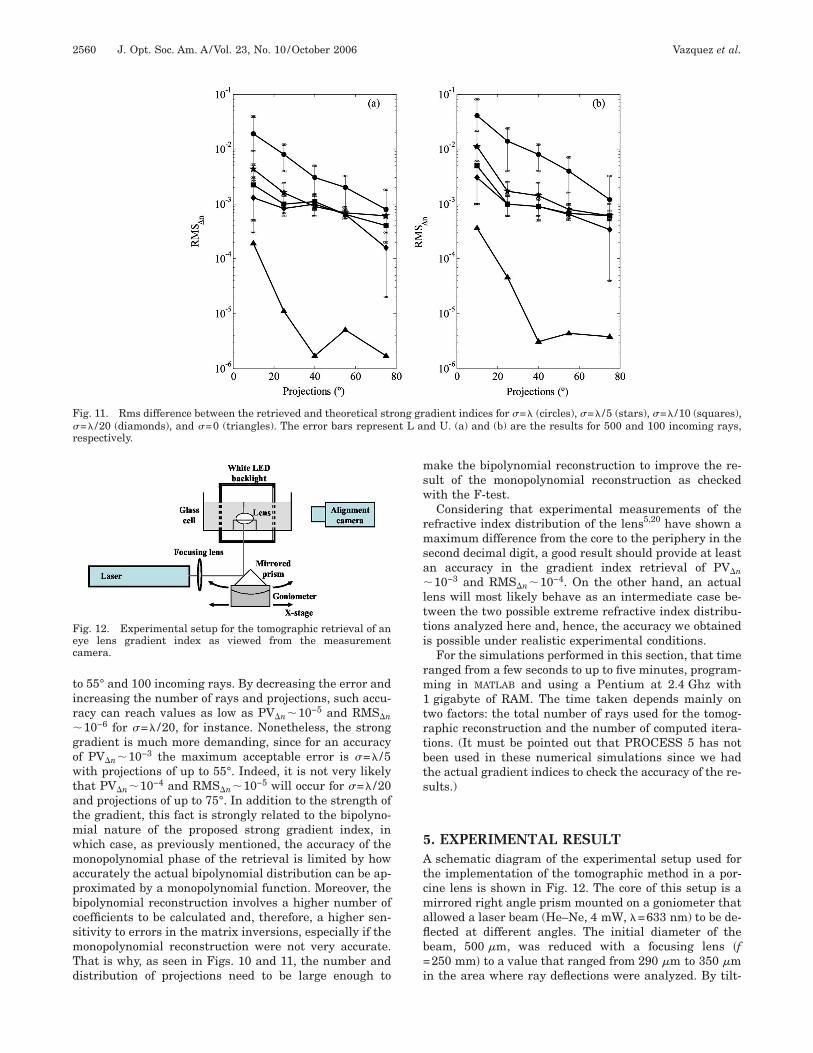
ig. 8. Peak–valley difference between the retrieved and theoreticalsquares), �= /20 (diamonds), and �=0 (triangles). The error bars reprng rays, respectively.

oo

aR

F�r

F=i

Vazquez et al. Vol. 23, No. 10 /October 2006 /J. Opt. Soc. Am. A 2559

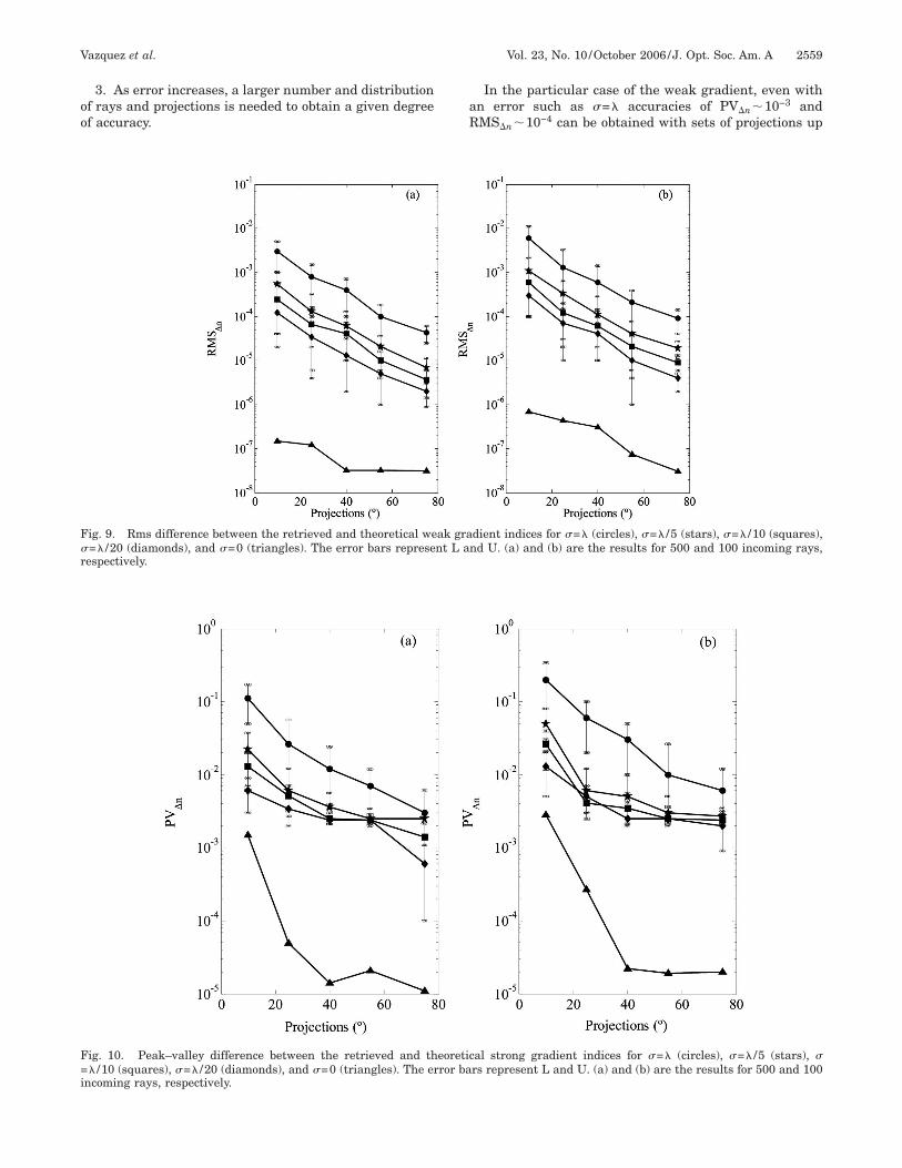
3. As error increases, a larger number and distributionf rays and projections is needed to obtain a given degreef accuracy.

ig. 9. Rms difference between the retrieved and theoretical we= /20 (diamonds), and �=0 (triangles). The error bars represeespectively.

ig. 10. Peak–valley difference between the retrieved and th /10 (squares), �= /20 (diamonds), and �=0 (triangles). The er

ncoming rays, respectively.

In the particular case of the weak gradient, even withn error such as �= accuracies of PV�n�10−3 andMS�n�10−4 can be obtained with sets of projections up

dient indices for �= (circles), �= /5 (stars), �= /10 (squares),nd U. (a) and (b) are the results for 500 and 100 incoming rays,

al strong gradient indices for �= (circles), �= /5 (stars), �rs represent L and U. (a) and (b) are the results for 500 and 100

ak grant L a

eoreticror ba

tir�gowtatmwmapbcsmTd

msw

rmsa�ltti

rm1trtbts

5Atcmaflb=i

F�r

Fec

2560 J. Opt. Soc. Am. A/Vol. 23, No. 10 /October 2006 Vazquez et al.

o 55° and 100 incoming rays. By decreasing the error andncreasing the number of rays and projections, such accu-acy can reach values as low as PV�n�10−5 and RMS�n10−6 for �= /20, for instance. Nonetheless, the strong

radient is much more demanding, since for an accuracyf PV�n�10−3 the maximum acceptable error is �= /5ith projections of up to 55°. Indeed, it is not very likely

hat PV�n�10−4 and RMS�n�10−5 will occur for �= /20nd projections of up to 75°. In addition to the strength ofhe gradient, this fact is strongly related to the bipolyno-ial nature of the proposed strong gradient index, inhich case, as previously mentioned, the accuracy of theonopolynomial phase of the retrieval is limited by how

ccurately the actual bipolynomial distribution can be ap-roximated by a monopolynomial function. Moreover, theipolynomial reconstruction involves a higher number ofoefficients to be calculated and, therefore, a higher sen-itivity to errors in the matrix inversions, especially if theonopolynomial reconstruction were not very accurate.hat is why, as seen in Figs. 10 and 11, the number andistribution of projections need to be large enough to

ig. 11. Rms difference between the retrieved and theoretical str= /20 (diamonds), and �=0 (triangles). The error bars represeespectively.

ig. 12. Experimental setup for the tomographic retrieval of anye lens gradient index as viewed from the measurementamera.

ake the bipolynomial reconstruction to improve the re-ult of the monopolynomial reconstruction as checkedith the F-test.Considering that experimental measurements of the

efractive index distribution of the lens5,20 have shown aaximum difference from the core to the periphery in the

econd decimal digit, a good result should provide at leastn accuracy in the gradient index retrieval of PV�n10−3 and RMS�n�10−4. On the other hand, an actual

ens will most likely behave as an intermediate case be-ween the two possible extreme refractive index distribu-ions analyzed here and, hence, the accuracy we obtaineds possible under realistic experimental conditions.

For the simulations performed in this section, that timeanged from a few seconds to up to five minutes, program-ing in MATLAB and using a Pentium at 2.4 Ghz withgigabyte of RAM. The time taken depends mainly on

wo factors: the total number of rays used for the tomog-aphic reconstruction and the number of computed itera-ions. (It must be pointed out that PROCESS 5 has noteen used in these numerical simulations since we hadhe actual gradient indices to check the accuracy of the re-ults.)

. EXPERIMENTAL RESULTschematic diagram of the experimental setup used for

he implementation of the tomographic method in a por-ine lens is shown in Fig. 12. The core of this setup is airrored right angle prism mounted on a goniometer that

llowed a laser beam (He–Ne, 4 mW, =633 nm) to be de-ected at different angles. The initial diameter of theeam, 500 m, was reduced with a focusing lens �f250 mm� to a value that ranged from 290 m to 350 m

n the area where ray deflections were analyzed. By tilt-

adient indices for �= (circles), �= /5 (stars), �= /10 (squares),nd U. (a) and (b) are the results for 500 and 100 incoming rays,

ong grnt L a

ibtabrww=vmllpotwppdmp1e�folflba

earutt�tctmtl

gtNeswipgs

tatawsdiraso=9

pitsoil=Dv

bfirttb

Fw

Fo�

Vazquez et al. Vol. 23, No. 10 /October 2006 /J. Opt. Soc. Am. A 2561

ng the prism and moving the goniometer forward and/orackward, the crystalline lens could be illuminated andhe data for one projection collected. The lens was heldgainst the central opening of a pedestal that lay on theottom surface of a glass cell placed over the prism. Sur-ounding the lens was a 0.9% sodium chloride solutionhose index at =633 nm and T=22.0 °C was measuredith an Abbe refractometer, providing a value of next1.3332. A few drops of milk were added to the solution toisualize the laser beams. In order to minimize misalign-ents, an alignment camera was used to check that the

aser beams passed through the meridional plane of theens under consideration, regardless of the inclination orosition of the prism. Such meridional plane was previ-usly found by using the alignment camera to search forhe plane orthogonal to the object plane of the cameraithin which the deflection of the incoming rays tooklace completely. Another camera, perpendicular to thelane depicted at Fig. 12, captured the images of the rayseflected by the lens that were later used for the imple-entation of the tomographic algorithm as previouly ex-

lained. This measurement camera had a CCD array of344�1024 pixels and a resolution of 12.7 m/pixel. Forach image, rectangular and consecutive regions of 1661024, 598�1024, and 580�1024 pixels were reserved

or the analysis of the incoming rays, lens surfaces, andutgoing rays, respectively. With the aim of reducing theevel of noise, three images were taken for each ray de-ection and subsequently averaged. Finally, a white LEDacklight behind the lens was used to obtain a sharp im-ge of its surface by contrast, as seen in Fig. 13.In order to minimize and take stock of the experimental

rrors of this apparatus in the optical characterization oflens, a spherical, homogeneous BK7 glass lens of known

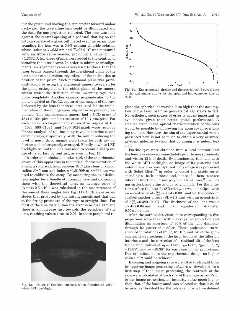
adius R=5 mm and index n=1.51509 at =633 nm wassed to calibrate the setup. By measuring the exit deflec-ion angles for a bundle of incoming rays and comparinghem with the theoretical ones, an average error of� sin�=2.5�10−3 was calculated in the measurement ofhe sine of those angles (see Fig. 14). Such an error in-ludes that produced by the misalignments and that dueo the fitting procedure of the rays to straight lines. Forost of the sine distribution the error is below 0.002 and

here is an increase just towards the periphery of theens, reaching values close to 0.01. In those peripheral re-

ig. 13. Image of the lens surfaces when illuminated with ahite LED backlight.

ions the spherical aberration is so high that the assump-ion of the laser beam as geometrical ray starts to fail.evertheless, such source of error is not so important in

ye lenses, given their better optical performance. Amaller error in the optical characterization of the lensould be possible by improving the accuracy in position-

ng the lens. However, the aim of the experimental resultresented here is not so much to obtain a very accurateradient index as to show that obtaining it is indeed fea-ible.

Porcine eyes were obtained from a local abattoir, andhe lens was removed immediately prior to measurementsnd within 12 h of death. By illuminating this lens withhe white LED backlight, an image of its posterior andnterior surfaces was captured. This image was processedith Sobel filters27 in order to detect the pixels corre-

ponding to both surfaces and, hence, fit them to threeifferent functional forms: polynomials, ellipses28 (includ-ng circles), and ellipses plus polynomials. For the ante-ior surface the best fit �SD=4.4 m� was an ellipse withn eccentricity of elens

ant =0.654±0.001 and for the posteriorurface another ellipse �SD=7.3 m� with an eccentricityf elens

pos =0.389±0.007. The thickness of the lens was t7.48±0.04 mm and its equatorial diameter.55±0.09 mm.After the surface detection, data corresponding to five

rojections were taken with 130 rays per projection andlluminating an aperture of 90% of the lens diameterhrough its posterior surface. These projections corre-ponded to rotations of 0°, 3°, 6°, 10°, and 14° of the goni-meter. The refractions of the laser beams at the differentnterfaces and the correction of a residual tilt of the lensed to final values of �1=−1.95°, �2=1.86°, �3=6.93°, �413.05°, and �5=19.38° for each one of the projections.ue to limitations in the experimental design no higheralues of � could be achieved.

Incoming and outgoing rays were fitted to straight linesy applying image processing software we developed. In arst step of that image processing, the centroids of theays were calculated at each row of the image array. Prioro the image processing, an intensity value much higherhan that of the background was selected so that it coulde used as threshold for the retrieval of what we defined

ig. 14. Experimental (circles) and theoretical (solid curve) sinef the exit angles at z= t for the spherical homogeneous lens at=0°.

acvctStatmatrv

swsatgtTesTcfdpdon

it

fawocttitl

cas

t

m

Fnrr

Fm

2562 J. Opt. Soc. Am. A/Vol. 23, No. 10 /October 2006 Vazquez et al.

s the ray’s borders. Once these borders were obtained,entroids were calculated at each row from the intensityalues of the pixels between. Hence, the fitting of thoseentroids to straight lines led to a first approximation ofhe geometrical ray corresponding to each laser beam.ince the calculation of each centroid must be done or-hogonally to the direction of propagation of the ray, theccuracy of the former procedure decreases as the slope ofhe rays decreases and the laser beam loses its ideal sym-etrical Gaussian shape. For that reason, it was used asfirst step of an iterative process in which at each itera-

ion the centroids were calculated orthogonally to the di-ection retrieved at the former step until the results con-erged.

Once the outgoing and incoming rays were fitted totraight lines their intersections with the lens surfacesere calculated in order to obtain the input data de-

cribed in the monopolynomial phase of the tomographiclgorithm (see Section 3) and start the gradient index re-rieval. Cubic splines and a subsequent numerical inte-ration were used for the integration of the distribution ofhe sine of the angles of deflection described in Eq. (5).he algorithm converged with 4 interpolated points. Asxplained in PROCESS 5, we checked how accurately theolution reproduced the experimental data (see Table 3).he values of the RMS� sin for any of the projectionslosely coincide with the average error �� sin� calculatedor the homogeneous ball; hence the tomographic proce-ure could be halted at this point. However, to check theerformance of the bipolynomial model of the gradient in-ex, a second phase was initiated and results showed thatptical properties were as good as those of the monopoly-omial model (see Table 3).Due to experimental error, the coefficients correspond-

ng to orders higher than M=1 in the refractive index dis-ribution [see Eq. (8a)–(8c)] were not significant, either

Table 3. Accuracy of the Monopolynominal andBipolynomial Retrievals of the Porcine

Lens Gradient Index

� (°)Accuracy

Parameters Monopolynomial Bipolynomial

−1.95 RMS� sina 2�10−3 2�10−3

PV� sina 6�10−3 5�10−3

RMS�S (mm)b 7�10−3 7�10−3

1.86 RMS� sin 1.4�10−3 1.4�10−3

PV� sin 6�10−3 7�10−3

RMS�S (mm) 4�10−3 4�10−3

6.93 RMS� sin 1.2�10−3 1.2�10−3

PV� sin 4�10−3 4�10−3

RMS�S (mm) 5�10−3 5�10−3

13.05 RMS� sin 2�10−3 1.7�10−3

PV� sin 9�10−3 8�10−3

RMS�S (mm) 7�10−3 7�10−3

19.38 RMS� sin 3�10−3 3�10−3

PV� sin 15�10−3 12�10−3

RMS�S (mm) 11�10−3 11�10−3

aRMS� sin and PV� sin are the rms and peak–valley values of the difference be-ween the reproduced and experimental exit angle sine distributions in all rows.

bRMS�S is the rms value of the difference between the reproduced and experi-ental optical path distributions in all rows.

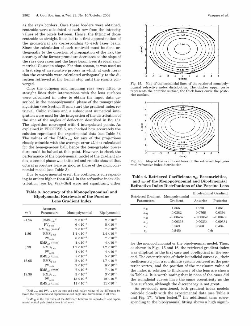
or the monopolynomial or the bipolynomial model. Thus,s shown in Figs. 15 and 16, the retrieved gradient indexas elliptical in the first case and bi-elliptical in the sec-nd. The eccentricitcies of their isoindicial curves en, theiroefficients nij for a coordinate system centered at the pos-erior vertex, and the position of the maximum value ofhe index in relation to thickness t of the lens are shownn Table 4. It is worth noting that in none of the cases didhe isoindicial curves have the same eccentricity as theens surfaces, although the discrepancy is not great.

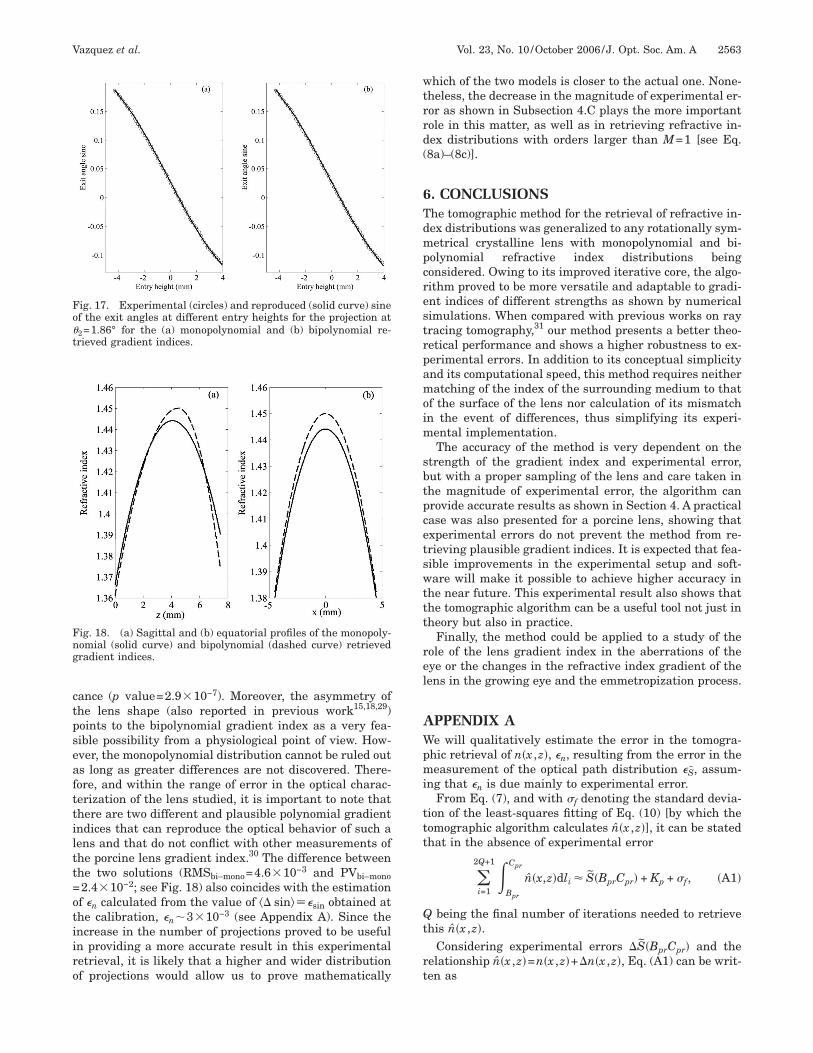
As previously mentioned, both gradient index modelsoincide closely with the experimental data (see Table 3nd Fig. 17). When tested,24 the additional term corre-ponding to the bipolynomial fitting shows a high signifi-

Table 4. Retrieved Coefficients nij, Eccentricities,and zH of the Monopolynomial and Bipolynomial

Refractive Index Distributions of the Porcine Lens

Retrieved GradientParameters

MonopolynomialGradient

Bipolynomial Gradient

Anterior Posterior

n00 1.366 1.278 1.361n01 0.0382 0.0766 0.0394n02 −0.00467 −0.00852 −0.00436n10 −0.00316 −0.00334 −0.00334en 0.569 0.780 0.484zH 0.545t 0.6t

ig. 15. Map of the isoindicial lines of the retrieved monopoly-omial refractive index distribution. The thicker upper curveepresents the anterior surface, the thick lower curve the poste-ior surface.

ig. 16. Map of the isoindicial lines of the retrieved bipolyno-ial refractive index distribution.

ctpseafttiltt=otiiro

wtrrd(

6Tdmpcrestrpamoim

sbtpcetswttt

rel

AWpmi

ttt

Qt

rt

Fo�t

Fng

Vazquez et al. Vol. 23, No. 10 /October 2006 /J. Opt. Soc. Am. A 2563

ance (p value=2.9�10−7). Moreover, the asymmetry ofhe lens shape (also reported in previous work15,18,29)oints to the bipolynomial gradient index as a very fea-ible possibility from a physiological point of view. How-ver, the monopolynomial distribution cannot be ruled outs long as greater differences are not discovered. There-ore, and within the range of error in the optical charac-erization of the lens studied, it is important to note thathere are two different and plausible polynomial gradientndices that can reproduce the optical behavior of such aens and that do not conflict with other measurements ofhe porcine lens gradient index.30 The difference betweenhe two solutions (RMSbi–mono=4.6�10−3 and PVbi–mono2.4�10−2; see Fig. 18) also coincides with the estimationf �n calculated from the value of �� sin���sin obtained athe calibration, �n�3�10−3 (see Appendix A). Since thencrease in the number of projections proved to be usefuln providing a more accurate result in this experimentaletrieval, it is likely that a higher and wider distributionf projections would allow us to prove mathematically

ig. 17. Experimental (circles) and reproduced (solid curve) sinef the exit angles at different entry heights for the projection at2=1.86° for the (a) monopolynomial and (b) bipolynomial re-rieved gradient indices.

ig. 18. (a) Sagittal and (b) equatorial profiles of the monopoly-omial (solid curve) and bipolynomial (dashed curve) retrievedradient indices.

hich of the two models is closer to the actual one. None-heless, the decrease in the magnitude of experimental er-or as shown in Subsection 4.C plays the more importantole in this matter, as well as in retrieving refractive in-ex distributions with orders larger than M=1 [see Eq.8a)–(8c)].

. CONCLUSIONShe tomographic method for the retrieval of refractive in-ex distributions was generalized to any rotationally sym-etrical crystalline lens with monopolynomial and bi-

olynomial refractive index distributions beingonsidered. Owing to its improved iterative core, the algo-ithm proved to be more versatile and adaptable to gradi-nt indices of different strengths as shown by numericalimulations. When compared with previous works on rayracing tomography,31 our method presents a better theo-etical performance and shows a higher robustness to ex-erimental errors. In addition to its conceptual simplicitynd its computational speed, this method requires neitheratching of the index of the surrounding medium to that

f the surface of the lens nor calculation of its mismatchn the event of differences, thus simplifying its experi-

ental implementation.The accuracy of the method is very dependent on the

trength of the gradient index and experimental error,ut with a proper sampling of the lens and care taken inhe magnitude of experimental error, the algorithm canrovide accurate results as shown in Section 4. A practicalase was also presented for a porcine lens, showing thatxperimental errors do not prevent the method from re-rieving plausible gradient indices. It is expected that fea-ible improvements in the experimental setup and soft-are will make it possible to achieve higher accuracy in

he near future. This experimental result also shows thathe tomographic algorithm can be a useful tool not just inheory but also in practice.

Finally, the method could be applied to a study of theole of the lens gradient index in the aberrations of theye or the changes in the refractive index gradient of theens in the growing eye and the emmetropization process.

PPENDIX Ae will qualitatively estimate the error in the tomogra-

hic retrieval of n�x ,z�, �n, resulting from the error in theeasurement of the optical path distribution �S, assum-

ng that �n is due mainly to experimental error.From Eq. (7), and with �f denoting the standard devia-

ion of the least-squares fitting of Eq. (10) [by which theomographic algorithm calculates n�x ,z�], it can be statedhat in the absence of experimental error

�i=1

2Q+1�Bpr

Cpr

n�x,z�dli S�BprCpr� + Kp + �f, �A1�

being the final number of iterations needed to retrievehis n�x ,z�.

Considering experimental errors �S�BprCpr� and theelationship n�x ,z�=n�x ,z�+�n�x ,z�, Eq. (A1) can be writ-en as

2

p

t

sat

w

itre

w

ATECgJwm

R

1

1

1

1

1

1

1

1

1

1

2

2

2

2

2

2

2

2

2

2564 J. Opt. Soc. Am. A/Vol. 23, No. 10 /October 2006 Vazquez et al.

�i=1

Q+1 ��Bpr

Cpr

n�x,z�dli +�Bpr

Cpr

�n�x,z�dli S�BprCpr� + �S�BprCpr� + Kp + �f. �A2�

Assuming that the approximation of the actual rayaths by straight line segments is able to establish that

�i=1

2Q+1�Bpr

Cpr

n�x,z�dli S�BprCpr� + Kp, �A3�

hen the following relationship is obtained:

�i=1

2Q+1�Bpr

Cpr

�n�x,z�dli �S�BprCpr� + �f. �A4�

Assuming that �n�x ,z� and �S�BprCpr� do not vary sub-tantially along the integration domain, i.e., �n�x ,z� �n

nd �S�BprCpr� �S, the following upper bound for the es-imation for �n can be given:

�n ��S + �f

t, �A5�

here t is the thickness of the lens.In the case that optical path distribution is obtained us-

ng a laser scanning technique, a similar reasoning tohat applied in Ref. 8 can be used to obtain the followingelationship between the error in the measurement of thexit deflection sine �sin and �n:

�n ��S + �f

t�

nextReq�sin + �f

t, �A6�

here Req is the equatorial radius of the lens.

CKNOWLEDGMENTShis study was supported by the Spanish Ministerio deducación y Ciencia, Plan Nacional de Investigaciónientífica, Desarrollo e Innovación Tecnológica �I+D+I�,rant AYA2004-07773-C02-02 and FEDER. We also thankosé Albino Vázquez Aldrey for his help in providing usith pigs’ eyes and Sergio Barbero for his useful com-ents.D. Vazquez’s email address is [email protected].

EFERENCES1. P. L. Chu, “Nondestructive measurements of index profile

of an optical fibre preform,” Electron. Lett. 13, 736–738(1977).

2. D. Marcuse, “Refractive index determination by thefocusing method,” Appl. Opt. 18, 9–13 (1979).

3. V. I. Vlad and N. Ionescu-Pallas, “New treatment of thefocusing method and tomography of the refractive indexdistribution of inhomogeneous optical components,” Opt.Eng. (Bellingham) 35, 1305–1310 (1996).

4. D. Y. C. Chan, J. P. Ennis, B. K. Pierscionek, and G. Smith,“Determination of the 3-D gradient refractive indices incrystalline lenses,” Appl. Opt. 27, 926–931 (1988).

5. B. K. Pierscionek and D. Y. C. Chan, “Refractive indexgradient of human lenses,” Optom. Vision Sci. 66, 822–829(1989).

6. L. F. Garner, G. Smith, S. Yao, and R. C. Augusteyn,“Gradient refractive index of the crystalline lens of theBlack Oreo Dory (Allocyttus Niger): comparison ofmagnetic resonance imaging (MRI) and laser ray-tracemethods,” Vision Res. 41, 973–979 (2001).

7. E. Acosta, R. Flores, D. Vazquez, S. Rios, L. F. Garner, andG. Smith, “Tomographic method for measurement of therefractive index profile of optical fibre preforms and rodGRIN lenses,” Jpn. J. Appl. Phys., Part 1 41, 4821–4824(2002).

8. E. Acosta, D. Vazquez, L. Garner, and G. Smith,“Tomographic method for measurement of the gradientrefractive index of the crystalline lens. I. The spherical fishlens,” J. Opt. Soc. Am. A 22, 424–433 (2005).

9. R. D. Fernald, “The optical system of the fish” in The VisualSystem of Fish, R. H. Douglas and M. B. A. Djamgoz, eds.(Chapman & Hall, 1990), pp. 50–52.

0. W. S. Jagger, “The optics of the spherical fish lens,” VisionRes. 32, 1271–1284 (1992).

1. J. G. Sivak, “Optical variability of the fish lens,” in Ref. 9,pp. 63–74.

2. M. C. W. Campbell, “Measurement of refractive index in anintact crystalline lens,” Vision Res. 24, 409–415 (1984).

3. K. F. Barrell and C. Pask, “Nondestructive index profilemeasurements of noncircular optical fibre preforms,” Opt.Commun. 27, 230–234 (1978).

4. G. Beliakov and D. Y. C. Chan, “Analysis of inhomogeneousoptical systems by the use of ray tracing. II. Three-dimensional systems with symmetry,” Appl. Opt. 37,5106–5111 (1998).

5. J. R. Kuszak, K. L. Peterson, and H. G. Brown, “Electronmicroscopy observations of the crystalline lens,” Microsc.Res. Tech. 33, 441–479 (1996).

6. D. T. Moore, “Design of singlets with continuously varyingindices of refraction,” J. Opt. Soc. Am. 61, 886–894(1971).

7. J. W. Blaker, “Toward an adaptive model of the humaneye,” J. Opt. Soc. Am. 70, 220–223 (1980).

8. G. Smith, B. K. Pierscionek, and D. A. Atchison, “Theoptical modelling of the human lens,” Ophthalmic Physiol.Opt. 11, 359–369 (1991).

9. E. W. Marchand, Gradient Index Optics (Academic Press,1978), Chap. 9, p. 99.

0. B. A. Moffat, D. A. Atchison, and J. M. Pope, “Age-relatedchanges in refractive index distribution and power of thehuman lens as measured by magnetic resonance micro-imaging in vitro,” Vision Res. 42, 1683–1693 (2002).

1. A. Gullstrand, Appendix II in Helmholtz’s Handbuch derPhysiologischen Optik, Vol. 1, 3rd ed. (English translationedited by J. P. Southall, Optical Society of America, Dover,1962), pp. 351–352.

2. L. Montagnino, “Ray tracing in homogeneous media,” J.Opt. Soc. Am. 58, 1667–1668 (1968).

3. A. Sharma, D. V. Kumar, and A. K. Ghatak, “Tracing raysthrough graded-index media: a new method,” Appl. Opt. 21,984–987 (1982).

4. P. R. Bevington and D. K. Robinson, Data Reduction andError Analysis for the Physical Sciences (McGraw-Hill,1992), Chap. 11, pp. 205–209.

5. H. L. Liou and N. A. Brennan, “Anatomically accurate,finite model eye for optical modeling,” J. Opt. Soc. Am. A14, 1684–1695 (1997).

6. J. F. Koretz, C. A. Cook, and P. L. Kaufman, “Aging of thehuman lens: changes in lens shape upon accommodationand with accommodative loss,” J. Opt. Soc. Am. A 19,144–151 (2002).

7. R. C. Gonzalez and R. E. Woods, Digital Image Processing(Addison-Wesley, 1993), Chap. 7, pp. 416–423.

8. R. Halír and J. Flusser, “Numerically stable direct leastsquares fitting of ellipses,” in Proceedings of the SixthInternational Conference in Central Europe on Computer

2

3

3

Vazquez et al. Vol. 23, No. 10 /October 2006 /J. Opt. Soc. Am. A 2565

Graphics and Visualization (WSCG’98), V. Skala, ed.(Vydavatelstvi Zapadoceske Univerzity, , 1998), Vol. 1, pp.125–132.

9. W. S. Jagger, “The refractive structure and opticalproperties of the isolated crystalline lens of the cat,” VisionRes. 30, 723–738 (1990).

0. C. E. Jones and J. M. Pope, “Measuring optical properties

of an eye lens using magnetic resonance imaging,” Magn.Reson. Imaging 22, 211–220 (2004).

1. S. Barbero, A. Glasser, C. Clark, and S. Marcos, “Accuracyand possibilities for evaluating the lens gradient-indexusing a ray tracing tomography global optimizationstrategy,” Invest. Ophthalmol. Visual Sci. 45 Suppl. 1,