Today: 5.4 General log and exp functions (continued) Warm up: log a (x) = ln(x)/ ln(a) d dx log a (x)= 1 ln(a)x 1. Evaluate the following functions. log 5 (25) log 7 √ 7 log 4 8 - log 4 2 2. Differentiate the following functions. log 10 x x log 2 (x) 2 x+log 3 (x) log 5 (x 2 + 1), x log e (x) - x, 3 x ln(x) , p 1 - (1/3) x 3. Calculate the following antiderivatives: Z 3 x 3 x +3 dx Z 2 1/x x 2 dx Z e x (3e x + 1) 1/3 dx Z 1 x ln(x) dx

Welcome message from author
This document is posted to help you gain knowledge. Please leave a comment to let me know what you think about it! Share it to your friends and learn new things together.
Transcript
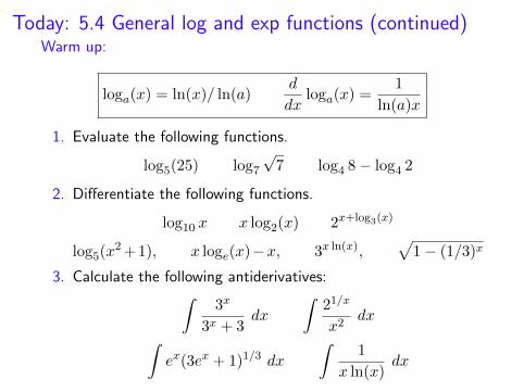
Today: 5.4 General log and exp functions (continued)Warm up:
loga(x) = ln(x)/ ln(a)d
dxloga(x) =
1
ln(a)x
1. Evaluate the following functions.
log5(25) log7√7 log4 8− log4 2
2. Differentiate the following functions.
log10 x x log2(x) 2x+log3(x)
log5(x2+1), x loge(x)−x, 3x ln(x),
√1− (1/3)x
3. Calculate the following antiderivatives:∫3x
3x + 3dx
∫21/x
x2dx∫
ex(3ex + 1)1/3 dx
∫1
x ln(x)dx
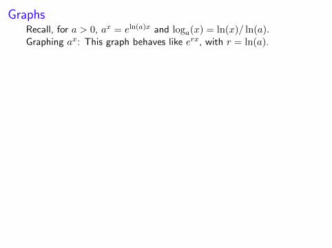
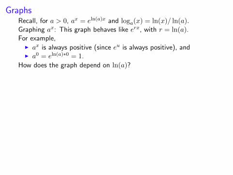
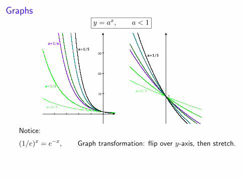
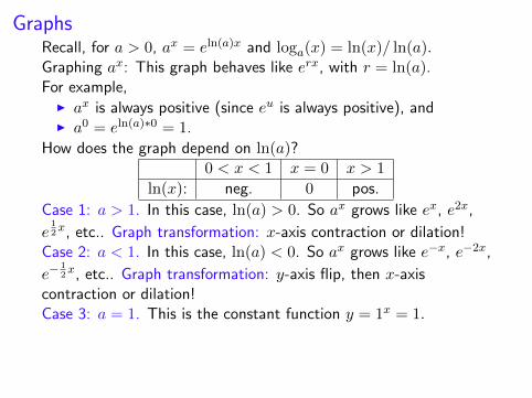
GraphsRecall, for a > 0, ax = eln(a)x and loga(x) = ln(x)/ ln(a).Graphing ax: This graph behaves like erx, with r = ln(a).
For example,I ax is always positive (since eu is always positive), andI a0 = eln(a)∗0 = 1.
How does the graph depend on ln(a)?0 < x < 1 x = 0 x > 1
ln(x): neg. 0 pos.
Case 1: a > 1. In this case, ln(a) > 0. So ax grows like ex, e2x,
e12x, etc.. Graph transformation: x-axis contraction or dilation!
Case 2: a < 1. In this case, ln(a) < 0. So ax grows like e−x, e−2x,
e−12x, etc.. Graph transformation: y-axis flip, then x-axis
contraction or dilation!Case 3: a = 1. This is the constant function y = 1x = 1.
Notice: Slope at x = 0 is
d
dxax∣∣x=0
= ln(a)ax∣∣x=0
= ln(a).
So y = ex is the exponential function whose slope through thepoint (0, 1) is 1. For a < e, the slope at x = 0 is less than 1, andfor a > e, the slope at x = 0 is greater than 1.
Notice:
(1/e)x = e−x, Graph transformation: flip over y-axis, then stretch.
So y = (1/e)x is the exponential function whose slope through thepoint (0, 1) is −1. For a < 1/e, the slope at x = 0 is less than −1,and for a > 1/e, the slope at x = 0 is greater than −1.

GraphsRecall, for a > 0, ax = eln(a)x and loga(x) = ln(x)/ ln(a).Graphing ax: This graph behaves like erx, with r = ln(a).For example,
I ax is always positive (since eu is always positive), andI a0 = eln(a)∗0 = 1.
How does the graph depend on ln(a)?0 < x < 1 x = 0 x > 1
ln(x): neg. 0 pos.
Case 1: a > 1. In this case, ln(a) > 0. So ax grows like ex, e2x,
e12x, etc.. Graph transformation: x-axis contraction or dilation!
Case 2: a < 1. In this case, ln(a) < 0. So ax grows like e−x, e−2x,
e−12x, etc.. Graph transformation: y-axis flip, then x-axis
contraction or dilation!Case 3: a = 1. This is the constant function y = 1x = 1.
Notice: Slope at x = 0 is
d
dxax∣∣x=0
= ln(a)ax∣∣x=0
= ln(a).
So y = ex is the exponential function whose slope through thepoint (0, 1) is 1. For a < e, the slope at x = 0 is less than 1, andfor a > e, the slope at x = 0 is greater than 1.
Notice:
(1/e)x = e−x, Graph transformation: flip over y-axis, then stretch.
So y = (1/e)x is the exponential function whose slope through thepoint (0, 1) is −1. For a < 1/e, the slope at x = 0 is less than −1,and for a > 1/e, the slope at x = 0 is greater than −1.
GraphsRecall, for a > 0, ax = eln(a)x and loga(x) = ln(x)/ ln(a).Graphing ax: This graph behaves like erx, with r = ln(a).For example,
I ax is always positive (since eu is always positive), andI a0 = eln(a)∗0 = 1.
How does the graph depend on ln(a)?
0 < x < 1 x = 0 x > 1
ln(x): neg. 0 pos.
Case 1: a > 1. In this case, ln(a) > 0. So ax grows like ex, e2x,
e12x, etc.. Graph transformation: x-axis contraction or dilation!
Case 2: a < 1. In this case, ln(a) < 0. So ax grows like e−x, e−2x,
e−12x, etc.. Graph transformation: y-axis flip, then x-axis
contraction or dilation!Case 3: a = 1. This is the constant function y = 1x = 1.
Notice: Slope at x = 0 is
d
dxax∣∣x=0
= ln(a)ax∣∣x=0
= ln(a).
So y = ex is the exponential function whose slope through thepoint (0, 1) is 1. For a < e, the slope at x = 0 is less than 1, andfor a > e, the slope at x = 0 is greater than 1.
Notice:
(1/e)x = e−x, Graph transformation: flip over y-axis, then stretch.
So y = (1/e)x is the exponential function whose slope through thepoint (0, 1) is −1. For a < 1/e, the slope at x = 0 is less than −1,and for a > 1/e, the slope at x = 0 is greater than −1.

GraphsRecall, for a > 0, ax = eln(a)x and loga(x) = ln(x)/ ln(a).Graphing ax: This graph behaves like erx, with r = ln(a).For example,
I ax is always positive (since eu is always positive), andI a0 = eln(a)∗0 = 1.
How does the graph depend on ln(a)?0 < x < 1 x = 0 x > 1
ln(x): neg. 0 pos.
Case 1: a > 1. In this case, ln(a) > 0. So ax grows like ex, e2x,
e12x, etc.. Graph transformation: x-axis contraction or dilation!
Case 2: a < 1. In this case, ln(a) < 0. So ax grows like e−x, e−2x,
e−12x, etc.. Graph transformation: y-axis flip, then x-axis
contraction or dilation!Case 3: a = 1. This is the constant function y = 1x = 1.
Notice: Slope at x = 0 is
d
dxax∣∣x=0
= ln(a)ax∣∣x=0
= ln(a).
So y = ex is the exponential function whose slope through thepoint (0, 1) is 1. For a < e, the slope at x = 0 is less than 1, andfor a > e, the slope at x = 0 is greater than 1.
Notice:
(1/e)x = e−x, Graph transformation: flip over y-axis, then stretch.
So y = (1/e)x is the exponential function whose slope through thepoint (0, 1) is −1. For a < 1/e, the slope at x = 0 is less than −1,and for a > 1/e, the slope at x = 0 is greater than −1.
GraphsRecall, for a > 0, ax = eln(a)x and loga(x) = ln(x)/ ln(a).Graphing ax: This graph behaves like erx, with r = ln(a).For example,
I ax is always positive (since eu is always positive), andI a0 = eln(a)∗0 = 1.
How does the graph depend on ln(a)?0 < x < 1 x = 0 x > 1
ln(x): neg. 0 pos.
Case 1: a > 1. In this case, ln(a) > 0. So ax grows like ex, e2x,
e12x, etc.. Graph transformation: x-axis contraction or dilation!
Case 2: a < 1. In this case, ln(a) < 0. So ax grows like e−x, e−2x,
e−12x, etc.. Graph transformation: y-axis flip, then x-axis
contraction or dilation!Case 3: a = 1. This is the constant function y = 1x = 1.
Notice: Slope at x = 0 is
d
dxax∣∣x=0
= ln(a)ax∣∣x=0
= ln(a).
So y = ex is the exponential function whose slope through thepoint (0, 1) is 1. For a < e, the slope at x = 0 is less than 1, andfor a > e, the slope at x = 0 is greater than 1.
Notice:
(1/e)x = e−x, Graph transformation: flip over y-axis, then stretch.
So y = (1/e)x is the exponential function whose slope through thepoint (0, 1) is −1. For a < 1/e, the slope at x = 0 is less than −1,and for a > 1/e, the slope at x = 0 is greater than −1.

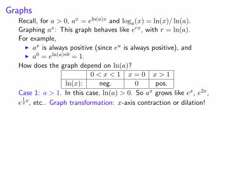
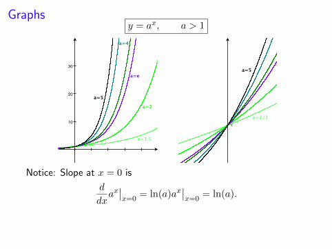
Graphsy = ax, a > 1
10
20
30
a=2
a=e
a=5
a=1.5
a=4
1
a=5
a=2/3
Notice: Slope at x = 0 is
d
dxax∣∣x=0
= ln(a)ax∣∣x=0
= ln(a).
So y = ex is the exponential function whose slope through thepoint (0, 1) is 1. For a < e, the slope at x = 0 is less than 1, andfor a > e, the slope at x = 0 is greater than 1.
Notice:
(1/e)x = e−x, Graph transformation: flip over y-axis, then stretch.
So y = (1/e)x is the exponential function whose slope through thepoint (0, 1) is −1. For a < 1/e, the slope at x = 0 is less than −1,and for a > 1/e, the slope at x = 0 is greater than −1.
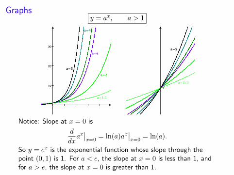
Graphsy = ax, a > 1
10
20
30
a=2
a=e
a=5
a=1.5
a=4
1
a=5
a=2/3
Notice: Slope at x = 0 is
d
dxax∣∣x=0
= ln(a)ax∣∣x=0
= ln(a).
So y = ex is the exponential function whose slope through thepoint (0, 1) is 1. For a < e, the slope at x = 0 is less than 1, andfor a > e, the slope at x = 0 is greater than 1. Notice:
(1/e)x = e−x, Graph transformation: flip over y-axis, then stretch.
So y = (1/e)x is the exponential function whose slope through thepoint (0, 1) is −1. For a < 1/e, the slope at x = 0 is less than −1,and for a > 1/e, the slope at x = 0 is greater than −1.
Graphsy = ax, a > 1
10
20
30
a=2
a=e
a=5
a=1.5
a=4
1
a=5
a=2/3
Notice: Slope at x = 0 is
d
dxax∣∣x=0
= ln(a)ax∣∣x=0
= ln(a).
So y = ex is the exponential function whose slope through thepoint (0, 1) is 1. For a < e, the slope at x = 0 is less than 1, andfor a > e, the slope at x = 0 is greater than 1.
Notice:
(1/e)x = e−x, Graph transformation: flip over y-axis, then stretch.
So y = (1/e)x is the exponential function whose slope through thepoint (0, 1) is −1. For a < 1/e, the slope at x = 0 is less than −1,and for a > 1/e, the slope at x = 0 is greater than −1.

GraphsRecall, for a > 0, ax = eln(a)x and loga(x) = ln(x)/ ln(a).Graphing ax: This graph behaves like erx, with r = ln(a).For example,
I ax is always positive (since eu is always positive), andI a0 = eln(a)∗0 = 1.
How does the graph depend on ln(a)?0 < x < 1 x = 0 x > 1
ln(x): neg. 0 pos.
Case 1: a > 1. In this case, ln(a) > 0. So ax grows like ex, e2x,
e12x, etc.. Graph transformation: x-axis contraction or dilation!
Case 2: a < 1. In this case, ln(a) < 0.
So ax grows like e−x, e−2x,
e−12x, etc.. Graph transformation: y-axis flip, then x-axis
contraction or dilation!Case 3: a = 1. This is the constant function y = 1x = 1.
Notice: Slope at x = 0 is
d
dxax∣∣x=0
= ln(a)ax∣∣x=0
= ln(a).
So y = ex is the exponential function whose slope through thepoint (0, 1) is 1. For a < e, the slope at x = 0 is less than 1, andfor a > e, the slope at x = 0 is greater than 1.
Notice:
(1/e)x = e−x, Graph transformation: flip over y-axis, then stretch.
So y = (1/e)x is the exponential function whose slope through thepoint (0, 1) is −1. For a < 1/e, the slope at x = 0 is less than −1,and for a > 1/e, the slope at x = 0 is greater than −1.
Graphs
Notice: Slope at x = 0 is
d
dxax∣∣x=0
= ln(a)ax∣∣x=0
= ln(a).
So y = ex is the exponential function whose slope through thepoint (0, 1) is 1. For a < e, the slope at x = 0 is less than 1, andfor a > e, the slope at x = 0 is greater than 1.
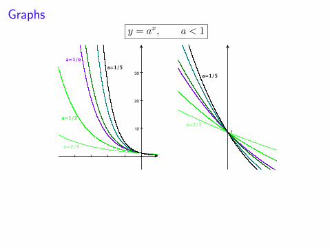
y = ax, a < 1
10
20
30
a=1/2
a=1/ea=1/5
a=2/3
1
a=1/5
a=2/3
Notice:
(1/e)x = e−x, Graph transformation: flip over y-axis, then stretch.
So y = (1/e)x is the exponential function whose slope through thepoint (0, 1) is −1. For a < 1/e, the slope at x = 0 is less than −1,and for a > 1/e, the slope at x = 0 is greater than −1.
Graphs
Notice: Slope at x = 0 is
d
dxax∣∣x=0
= ln(a)ax∣∣x=0
= ln(a).
So y = ex is the exponential function whose slope through thepoint (0, 1) is 1. For a < e, the slope at x = 0 is less than 1, andfor a > e, the slope at x = 0 is greater than 1.
y = ax, a < 1
10
20
30
a=1/2
a=1/ea=1/5
a=2/3
1
a=1/5
a=2/3
Notice:
(1/e)x = e−x, Graph transformation: flip over y-axis, then stretch.
So y = (1/e)x is the exponential function whose slope through thepoint (0, 1) is −1. For a < 1/e, the slope at x = 0 is less than −1,and for a > 1/e, the slope at x = 0 is greater than −1.
GraphsRecall, for a > 0, ax = eln(a)x and loga(x) = ln(x)/ ln(a).Graphing ax: This graph behaves like erx, with r = ln(a).For example,
I ax is always positive (since eu is always positive), andI a0 = eln(a)∗0 = 1.
How does the graph depend on ln(a)?0 < x < 1 x = 0 x > 1
ln(x): neg. 0 pos.
Case 1: a > 1. In this case, ln(a) > 0. So ax grows like ex, e2x,
e12x, etc.. Graph transformation: x-axis contraction or dilation!
Case 2: a < 1. In this case, ln(a) < 0. So ax grows like e−x, e−2x,
e−12x, etc.. Graph transformation: y-axis flip, then x-axis
contraction or dilation!Case 3: a = 1. This is the constant function y = 1x = 1.
Notice: Slope at x = 0 is
d
dxax∣∣x=0
= ln(a)ax∣∣x=0
= ln(a).
So y = ex is the exponential function whose slope through thepoint (0, 1) is 1. For a < e, the slope at x = 0 is less than 1, andfor a > e, the slope at x = 0 is greater than 1.
Notice:
(1/e)x = e−x, Graph transformation: flip over y-axis, then stretch.
So y = (1/e)x is the exponential function whose slope through thepoint (0, 1) is −1. For a < 1/e, the slope at x = 0 is less than −1,and for a > 1/e, the slope at x = 0 is greater than −1.
Graphs
10
a=5
a=1
a=1/5
a=2a=1/2
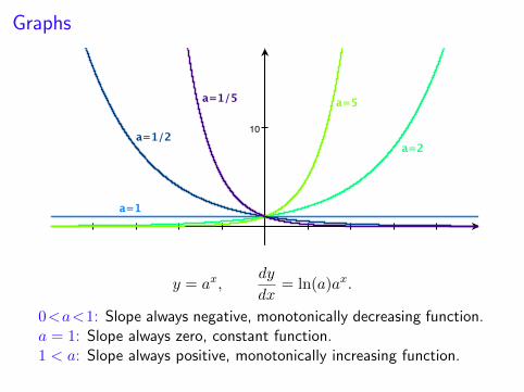
y = ax,dy
dx= ln(a)ax.
0<a<1: Slope always negative, monotonically decreasing function.a = 1: Slope always zero, constant function.1 < a: Slope always positive, monotonically increasing function.
You try:
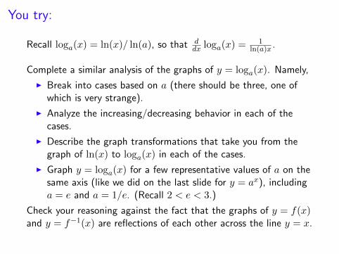
Recall loga(x) = ln(x)/ ln(a), so that ddx loga(x) =
1ln(a)x .
Complete a similar analysis of the graphs of y = loga(x). Namely,
I Break into cases based on a (there should be three, one ofwhich is very strange).
I Analyze the increasing/decreasing behavior in each of thecases.
I Describe the graph transformations that take you from thegraph of ln(x) to loga(x) in each of the cases.
I Graph y = loga(x) for a few representative values of a on thesame axis (like we did on the last slide for y = ax), includinga = e and a = 1/e. (Recall 2 < e < 3.)
Check your reasoning against the fact that the graphs of y = f(x)and y = f−1(x) are reflections of each other across the line y = x.

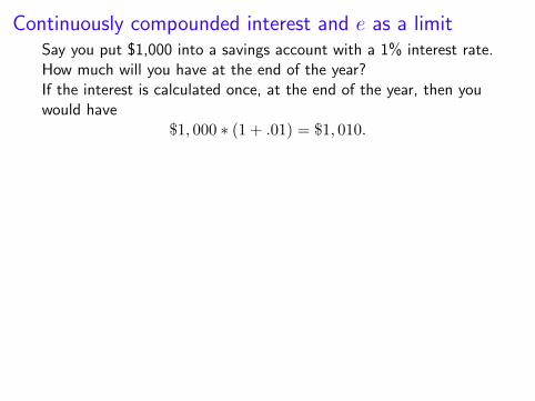
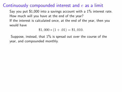
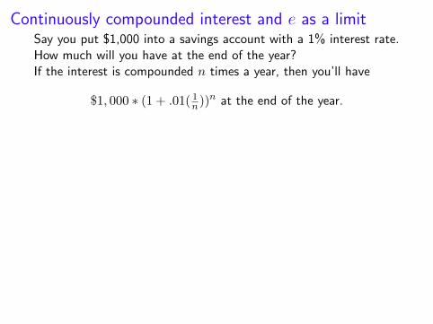
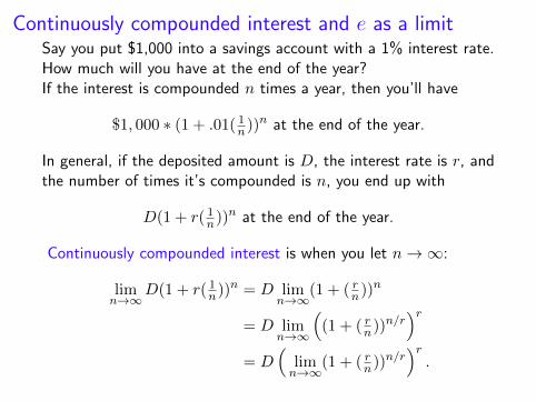
Continuously compounded interest and e as a limitSay you put $1,000 into a savings account with a 1% interest rate.How much will you have at the end of the year?
If the interest is calculated once, at the end of the year, then youwould have
$1, 000 ∗ (1 + .01) = $1, 010.
Suppose, instead, that 1% is spread out over the course of theyear, and compounded monthly. Then you’ll have
$1, 000 ∗ (1 + .01( 112)) = $1, 000.833 at the end of month 1,
$1, 000 ∗ (1 + .01( 112))
2 = $1, 001.667 at the end of month 2,
$1, 000 ∗ (1 + .01( 112))
3 = $1, 002.502 at the end of month 3,
...
$1, 000 ∗ (1 + .01( 112))
12 = $1, 010.046 at the end of month 12.,
i.e. a whole 4.6 cents more than if it had been compounded at theend of the year.
Continuously compounded interest and e as a limitSay you put $1,000 into a savings account with a 1% interest rate.How much will you have at the end of the year?If the interest is calculated once, at the end of the year, then youwould have
$1, 000 ∗ (1 + .01) = $1, 010.
Suppose, instead, that 1% is spread out over the course of theyear, and compounded monthly.
Then you’ll have
$1, 000 ∗ (1 + .01( 112)) = $1, 000.833 at the end of month 1,
$1, 000 ∗ (1 + .01( 112))
2 = $1, 001.667 at the end of month 2,
$1, 000 ∗ (1 + .01( 112))
3 = $1, 002.502 at the end of month 3,
...
$1, 000 ∗ (1 + .01( 112))
12 = $1, 010.046 at the end of month 12.,
i.e. a whole 4.6 cents more than if it had been compounded at theend of the year.

Continuously compounded interest and e as a limitSay you put $1,000 into a savings account with a 1% interest rate.How much will you have at the end of the year?If the interest is calculated once, at the end of the year, then youwould have
$1, 000 ∗ (1 + .01) = $1, 010.
Suppose, instead, that 1% is spread out over the course of theyear, and compounded monthly. Then you’ll have
$1, 000 ∗ (1 + .01( 112)) = $1, 000.833 at the end of month 1,
$1, 000 ∗ (1 + .01( 112))
2 = $1, 001.667 at the end of month 2,
$1, 000 ∗ (1 + .01( 112))
3 = $1, 002.502 at the end of month 3,
...
$1, 000 ∗ (1 + .01( 112))
12 = $1, 010.046 at the end of month 12.,
i.e. a whole 4.6 cents more than if it had been compounded at theend of the year.
Continuously compounded interest and e as a limitSay you put $1,000 into a savings account with a 1% interest rate.How much will you have at the end of the year?If the interest is calculated once, at the end of the year, then youwould have
$1, 000 ∗ (1 + .01) = $1, 010.
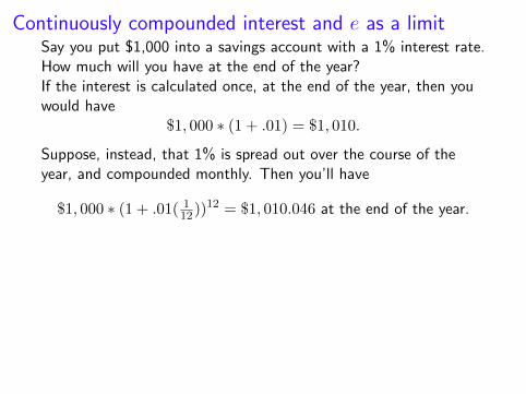
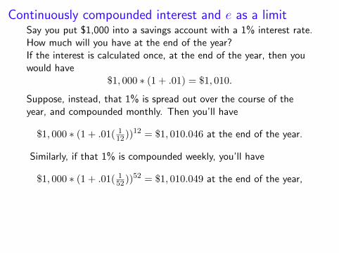
Suppose, instead, that 1% is spread out over the course of theyear, and compounded monthly. Then you’ll have
$1, 000 ∗ (1 + .01( 112))
12 = $1, 010.046 at the end of the year.
Similarly, if that 1% is compounded weekly, you’ll have
$1, 000 ∗ (1 + .01( 152))
52 = $1, 010.049 at the end of the year,
or compounded daily, you’ll have
$1, 000 ∗ (1 + .01( 1365))
365 = $1, 010.050 at the end of the year,
and so on.
Continuously compounded interest and e as a limitSay you put $1,000 into a savings account with a 1% interest rate.How much will you have at the end of the year?If the interest is calculated once, at the end of the year, then youwould have
$1, 000 ∗ (1 + .01) = $1, 010.
Suppose, instead, that 1% is spread out over the course of theyear, and compounded monthly. Then you’ll have
$1, 000 ∗ (1 + .01( 112))
12 = $1, 010.046 at the end of the year.
Similarly, if that 1% is compounded weekly, you’ll have
$1, 000 ∗ (1 + .01( 152))
52 = $1, 010.049 at the end of the year,
or compounded daily, you’ll have
$1, 000 ∗ (1 + .01( 1365))
365 = $1, 010.050 at the end of the year,
and so on.
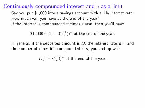
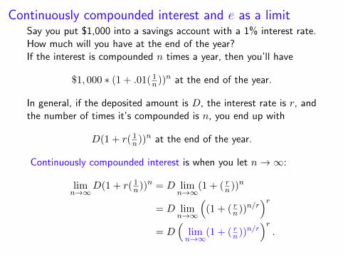
Continuously compounded interest and e as a limitSay you put $1,000 into a savings account with a 1% interest rate.How much will you have at the end of the year?If the interest is compounded n times a year, then you’ll have
$1, 000 ∗ (1 + .01( 1n))n at the end of the year.
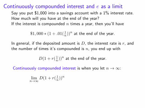
In general, if the deposited amount is D, the interest rate is r, andthe number of times it’s compounded is n, you end up with
D(1 + r( 1n))n at the end of the year.
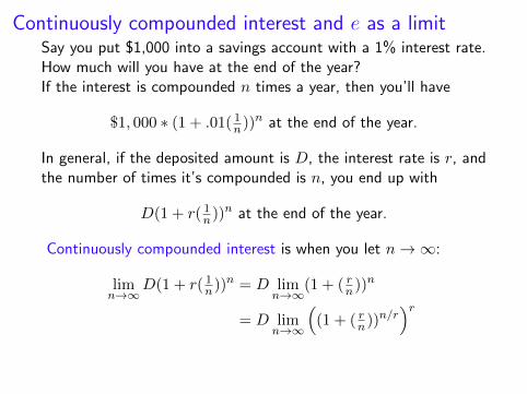
Continuously compounded interest is when you let n→∞:
limn→∞
D(1 + r( 1n))n = D lim
n→∞(1 + ( rn))
n
= D limn→∞
((1 + ( rn))
n/r)r
= D(
limn→∞
(1 + ( rn))n/r)r
.
Continuously compounded interest and e as a limitSay you put $1,000 into a savings account with a 1% interest rate.How much will you have at the end of the year?If the interest is compounded n times a year, then you’ll have
$1, 000 ∗ (1 + .01( 1n))n at the end of the year.
In general, if the deposited amount is D, the interest rate is r, andthe number of times it’s compounded is n, you end up with
D(1 + r( 1n))n at the end of the year.
Continuously compounded interest is when you let n→∞:
limn→∞
D(1 + r( 1n))n = D lim
n→∞(1 + ( rn))
n
= D limn→∞
((1 + ( rn))
n/r)r
= D(
limn→∞
(1 + ( rn))n/r)r
.
Continuously compounded interest and e as a limitSay you put $1,000 into a savings account with a 1% interest rate.How much will you have at the end of the year?If the interest is compounded n times a year, then you’ll have
$1, 000 ∗ (1 + .01( 1n))n at the end of the year.
In general, if the deposited amount is D, the interest rate is r, andthe number of times it’s compounded is n, you end up with
D(1 + r( 1n))n at the end of the year.
Continuously compounded interest is when you let n→∞:
limn→∞
D(1 + r( 1n))n
= D limn→∞
(1 + ( rn))n
= D limn→∞
((1 + ( rn))
n/r)r
= D(
limn→∞
(1 + ( rn))n/r)r
.

Continuously compounded interest and e as a limitSay you put $1,000 into a savings account with a 1% interest rate.How much will you have at the end of the year?If the interest is compounded n times a year, then you’ll have
$1, 000 ∗ (1 + .01( 1n))n at the end of the year.
In general, if the deposited amount is D, the interest rate is r, andthe number of times it’s compounded is n, you end up with
D(1 + r( 1n))n at the end of the year.
Continuously compounded interest is when you let n→∞:
limn→∞
D(1 + r( 1n))n = D lim
n→∞(1 + ( rn))
n
= D limn→∞
((1 + ( rn))
n/r)r
= D(
limn→∞
(1 + ( rn))n/r)r
.
Continuously compounded interest and e as a limitSay you put $1,000 into a savings account with a 1% interest rate.How much will you have at the end of the year?If the interest is compounded n times a year, then you’ll have
$1, 000 ∗ (1 + .01( 1n))n at the end of the year.
In general, if the deposited amount is D, the interest rate is r, andthe number of times it’s compounded is n, you end up with
D(1 + r( 1n))n at the end of the year.
Continuously compounded interest is when you let n→∞:
limn→∞
D(1 + r( 1n))n = D lim
n→∞(1 + ( rn))
n
= D limn→∞
((1 + ( rn))
n/r)r
= D(
limn→∞
(1 + ( rn))n/r)r
.
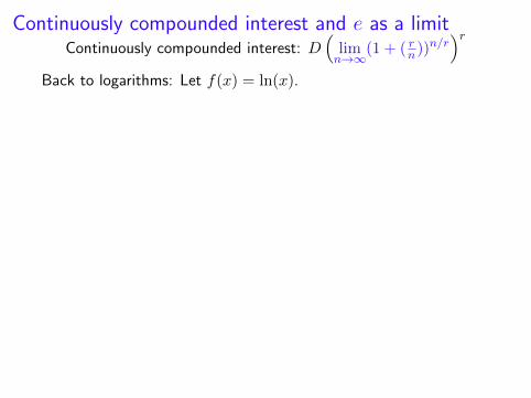
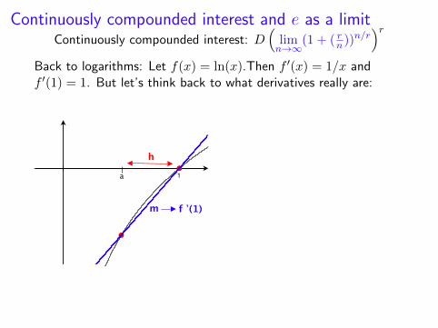
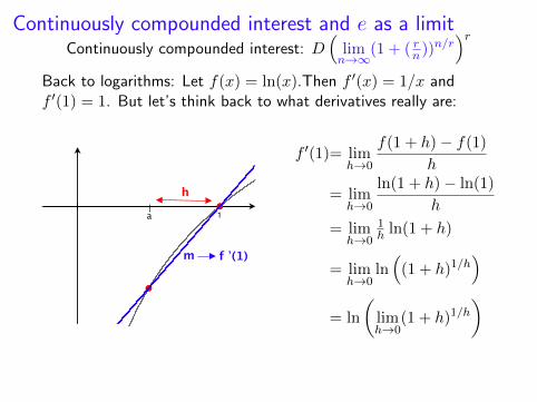
Continuously compounded interest and e as a limitContinuously compounded interest: D
(limn→∞
(1 + ( rn))n/r)r
Back to logarithms: Let f(x) = ln(x).
Then f ′(x) = 1/x andf ′(1) = 1. But let’s think back to what derivatives really are:
1
h
m f ’(1)
a
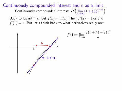
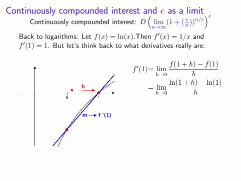
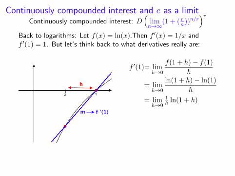
f ′(1)= limh→0
f(1 + h)− f(1)
h
= limh→0
ln(1 + h)− ln(1)
h
= limh→0
1h ln(1 + h)
= limh→0
ln((1 + h)1/h
)= ln
(limh→0
(1 + h)1/h)
Since 1 = ln
(limh→0
(1 + h)1/h), we have e = lim
h→0(1 + h)1/h .
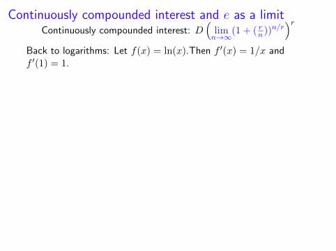
Continuously compounded interest and e as a limitContinuously compounded interest: D
(limn→∞
(1 + ( rn))n/r)r
Back to logarithms: Let f(x) = ln(x).Then f ′(x) = 1/x andf ′(1) = 1.
But let’s think back to what derivatives really are:
1
h
m f ’(1)
a
f ′(1)= limh→0
f(1 + h)− f(1)
h
= limh→0
ln(1 + h)− ln(1)
h
= limh→0
1h ln(1 + h)
= limh→0
ln((1 + h)1/h
)= ln
(limh→0
(1 + h)1/h)
Since 1 = ln
(limh→0
(1 + h)1/h), we have e = lim
h→0(1 + h)1/h .
Continuously compounded interest and e as a limitContinuously compounded interest: D
(limn→∞
(1 + ( rn))n/r)r
Back to logarithms: Let f(x) = ln(x).Then f ′(x) = 1/x andf ′(1) = 1. But let’s think back to what derivatives really are:
1
h
m f ’(1)
a
f ′(1)= limh→0
f(1 + h)− f(1)
h
= limh→0
ln(1 + h)− ln(1)
h
= limh→0
1h ln(1 + h)
= limh→0
ln((1 + h)1/h
)= ln
(limh→0
(1 + h)1/h)
Since 1 = ln
(limh→0
(1 + h)1/h), we have e = lim
h→0(1 + h)1/h .

Continuously compounded interest and e as a limitContinuously compounded interest: D
(limn→∞
(1 + ( rn))n/r)r
Back to logarithms: Let f(x) = ln(x).Then f ′(x) = 1/x andf ′(1) = 1. But let’s think back to what derivatives really are:
1
h
m f ’(1)
a
f ′(1)= limh→0
f(1 + h)− f(1)
h
= limh→0
ln(1 + h)− ln(1)
h
= limh→0
1h ln(1 + h)
= limh→0
ln((1 + h)1/h
)
= ln
(limh→0
(1 + h)1/h)
Since 1 = ln
(limh→0
(1 + h)1/h), we have e = lim
h→0(1 + h)1/h .
Continuously compounded interest and e as a limitContinuously compounded interest: D
(limn→∞
(1 + ( rn))n/r)r
Back to logarithms: Let f(x) = ln(x).Then f ′(x) = 1/x andf ′(1) = 1. But let’s think back to what derivatives really are:
1
h
m f ’(1)
a
f ′(1)= limh→0
f(1 + h)− f(1)
h
= limh→0
ln(1 + h)− ln(1)
h
= limh→0
1h ln(1 + h)
= limh→0
ln((1 + h)1/h
)= ln
(limh→0
(1 + h)1/h)
Since 1 = ln
(limh→0
(1 + h)1/h), we have e = lim
h→0(1 + h)1/h .

Continuously compounded interest and e as a limitContinuously compounded interest: D
(limn→∞
(1 + ( rn))n/r)r
Back to logarithms: Let f(x) = ln(x).Then f ′(x) = 1/x andf ′(1) = 1. But let’s think back to what derivatives really are:
1
h
m f ’(1)
a
f ′(1)= limh→0
f(1 + h)− f(1)
h
= limh→0
ln(1 + h)− ln(1)
h
= limh→0
1h ln(1 + h)
= limh→0
ln((1 + h)1/h
)= ln
(limh→0
(1 + h)1/h)
Since 1 = ln
(limh→0
(1 + h)1/h), we have e = lim
h→0(1 + h)1/h .

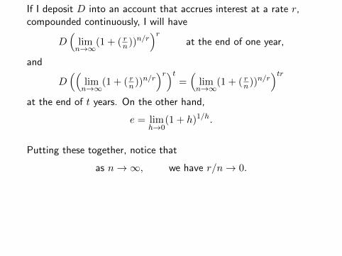
If I deposit D into an account that accrues interest at a rate r,compounded continuously, I will have
D(limn→∞
(1 + ( rn))n/r)r
at the end of one year,
and
D((
limn→∞
(1 + ( rn))n/r)r)t
=(limn→∞
(1 + ( rn))n/r)tr
at the end of t years. On the other hand,
e = limh→0
(1 + h)1/h.
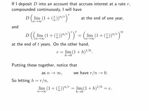
Putting these together, notice that
as n→∞, we have r/n→ 0.
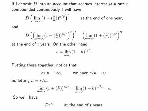
So letting h = r/n,
limn→∞
(1 + ( rn))n/r = lim
h→0(1 + h)1/h = e.
So we’ll have
Dert at the end of t years.

If I deposit D into an account that accrues interest at a rate r,compounded continuously, I will have
D(limn→∞
(1 + ( rn))n/r)r
at the end of one year,
and
D((
limn→∞
(1 + ( rn))n/r)r)t
=(limn→∞
(1 + ( rn))n/r)tr
at the end of t years.
On the other hand,
e = limh→0
(1 + h)1/h.
Putting these together, notice that
as n→∞, we have r/n→ 0.
So letting h = r/n,
limn→∞
(1 + ( rn))n/r = lim
h→0(1 + h)1/h = e.
So we’ll have
Dert at the end of t years.

If I deposit D into an account that accrues interest at a rate r,compounded continuously, I will have
D(limn→∞
(1 + ( rn))n/r)r
at the end of one year,
and
D((
limn→∞
(1 + ( rn))n/r)r)t
=(limn→∞
(1 + ( rn))n/r)tr
at the end of t years. On the other hand,
e = limh→0
(1 + h)1/h.
Putting these together, notice that
as n→∞, we have r/n→ 0.
So letting h = r/n,
limn→∞
(1 + ( rn))n/r = lim
h→0(1 + h)1/h = e.
So we’ll have
Dert at the end of t years.

5.5 Exponential growth and decay
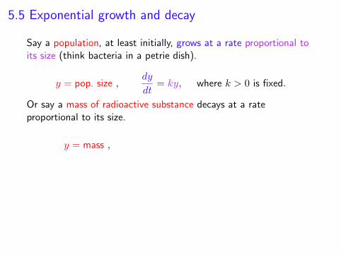
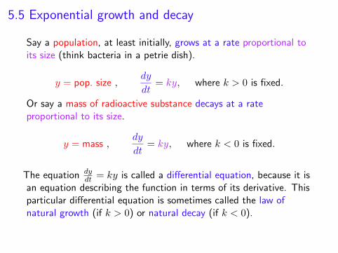
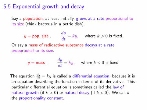
Say a population, at least initially, grows at a rate proportional toits size (think bacteria in a petrie dish).
y = pop. size ,dy
dt
= ky, where k > 0 is fixed.
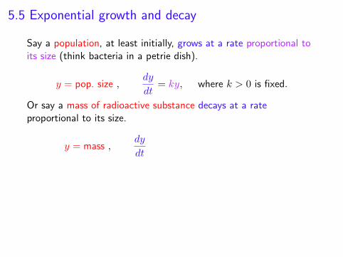
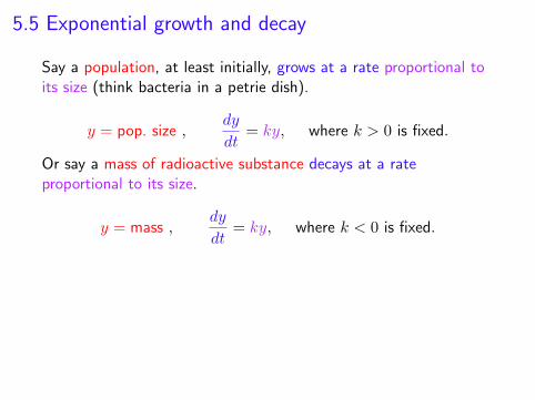
Or say a mass of radioactive substance decays at a rateproportional to its size.
y = mass ,dy
dt
= ky, where k < 0 is fixed.
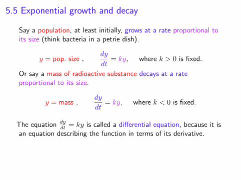
The equation dydt = ky is called a differential equation, because it is
an equation describing the function in terms of its derivative. Thisparticular differential equation is sometimes called the law ofnatural growth (if k > 0) or natural decay (if k < 0). We call kthe proportionality constant.
5.5 Exponential growth and decay
Say a population, at least initially, grows at a rate proportional toits size (think bacteria in a petrie dish).
y = pop. size ,
dy
dt
= ky, where k > 0 is fixed.
Or say a mass of radioactive substance decays at a rateproportional to its size.
y = mass ,dy
dt
= ky, where k < 0 is fixed.
The equation dydt = ky is called a differential equation, because it is
an equation describing the function in terms of its derivative. Thisparticular differential equation is sometimes called the law ofnatural growth (if k > 0) or natural decay (if k < 0). We call kthe proportionality constant.
5.5 Exponential growth and decay
Say a population, at least initially, grows at a rate proportional toits size (think bacteria in a petrie dish).
y = pop. size ,dy
dt
= ky, where k > 0 is fixed.
Or say a mass of radioactive substance decays at a rateproportional to its size.
y = mass ,dy
dt
= ky, where k < 0 is fixed.
The equation dydt = ky is called a differential equation, because it is
an equation describing the function in terms of its derivative. Thisparticular differential equation is sometimes called the law ofnatural growth (if k > 0) or natural decay (if k < 0). We call kthe proportionality constant.
5.5 Exponential growth and decay
Say a population, at least initially, grows at a rate proportional toits size (think bacteria in a petrie dish).
y = pop. size ,dy
dt= ky, where k > 0 is fixed.
Or say a mass of radioactive substance decays at a rateproportional to its size.
y = mass ,
dy
dt
= ky, where k < 0 is fixed.
The equation dydt = ky is called a differential equation, because it is
an equation describing the function in terms of its derivative. Thisparticular differential equation is sometimes called the law ofnatural growth (if k > 0) or natural decay (if k < 0). We call kthe proportionality constant.
5.5 Exponential growth and decay
Say a population, at least initially, grows at a rate proportional toits size (think bacteria in a petrie dish).
y = pop. size ,dy
dt= ky, where k > 0 is fixed.
Or say a mass of radioactive substance decays at a rateproportional to its size.
y = mass ,dy
dt
= ky, where k < 0 is fixed.
The equation dydt = ky is called a differential equation, because it is
an equation describing the function in terms of its derivative. Thisparticular differential equation is sometimes called the law ofnatural growth (if k > 0) or natural decay (if k < 0). We call kthe proportionality constant.
5.5 Exponential growth and decay
Say a population, at least initially, grows at a rate proportional toits size (think bacteria in a petrie dish).
y = pop. size ,dy
dt= ky, where k > 0 is fixed.
Or say a mass of radioactive substance decays at a rateproportional to its size.
y = mass ,dy
dt= ky, where k < 0 is fixed.
The equation dydt = ky is called a differential equation, because it is
an equation describing the function in terms of its derivative.
Thisparticular differential equation is sometimes called the law ofnatural growth (if k > 0) or natural decay (if k < 0). We call kthe proportionality constant.
5.5 Exponential growth and decay
Say a population, at least initially, grows at a rate proportional toits size (think bacteria in a petrie dish).
y = pop. size ,dy
dt= ky, where k > 0 is fixed.
Or say a mass of radioactive substance decays at a rateproportional to its size.
y = mass ,dy
dt= ky, where k < 0 is fixed.
The equation dydt = ky is called a differential equation, because it is
an equation describing the function in terms of its derivative. Thisparticular differential equation is sometimes called the law ofnatural growth (if k > 0) or natural decay (if k < 0).
We call kthe proportionality constant.
5.5 Exponential growth and decay
Say a population, at least initially, grows at a rate proportional toits size (think bacteria in a petrie dish).
y = pop. size ,dy
dt= ky, where k > 0 is fixed.
Or say a mass of radioactive substance decays at a rateproportional to its size.
y = mass ,dy
dt= ky, where k < 0 is fixed.
The equation dydt = ky is called a differential equation, because it is
an equation describing the function in terms of its derivative. Thisparticular differential equation is sometimes called the law ofnatural growth (if k > 0) or natural decay (if k < 0). We call kthe proportionality constant.
5.5 Exponential growth and decay
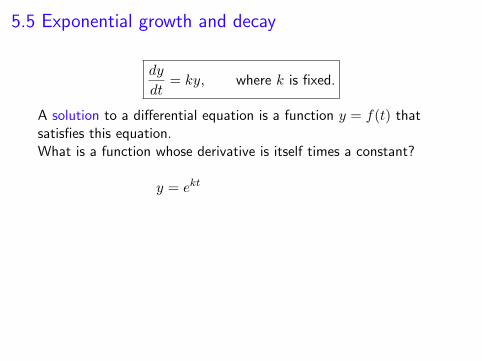
dy
dt= ky, where k is fixed.
A solution to a differential equation is a function y = f(t) thatsatisfies this equation.
What is a function whose derivative is itself times a constant?
y = ekt is one solution!
So are 2ekt, 3ekt, −ekt. . . Every solution looks like
y = Cekt where C and k are constant.
We call this the general solution. Notice that
y(0) = Ce0 = C.
5.5 Exponential growth and decay
dy
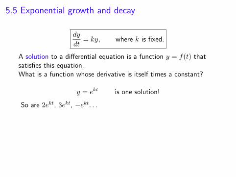
dt= ky, where k is fixed.
A solution to a differential equation is a function y = f(t) thatsatisfies this equation.What is a function whose derivative is itself times a constant?
y = ekt is one solution!
So are 2ekt, 3ekt, −ekt. . . Every solution looks like
y = Cekt where C and k are constant.
We call this the general solution. Notice that
y(0) = Ce0 = C.
5.5 Exponential growth and decay
dy
dt= ky, where k is fixed.
A solution to a differential equation is a function y = f(t) thatsatisfies this equation.What is a function whose derivative is itself times a constant?
y = ekt
is one solution!
So are 2ekt, 3ekt, −ekt. . . Every solution looks like
y = Cekt where C and k are constant.
We call this the general solution. Notice that
y(0) = Ce0 = C.
5.5 Exponential growth and decay
dy
dt= ky, where k is fixed.
A solution to a differential equation is a function y = f(t) thatsatisfies this equation.What is a function whose derivative is itself times a constant?
y = ekt is one solution!
So are 2ekt, 3ekt, −ekt. . .
Every solution looks like
y = Cekt where C and k are constant.
We call this the general solution. Notice that
y(0) = Ce0 = C.

5.5 Exponential growth and decay
dy
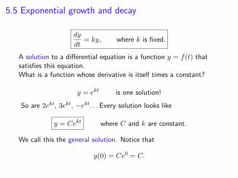
dt= ky, where k is fixed.
A solution to a differential equation is a function y = f(t) thatsatisfies this equation.What is a function whose derivative is itself times a constant?
y = ekt is one solution!
So are 2ekt, 3ekt, −ekt. . . Every solution looks like
y = Cekt where C and k are constant.
We call this the general solution.
Notice that
y(0) = Ce0 = C.
5.5 Exponential growth and decay
dy
dt= ky, where k is fixed.
A solution to a differential equation is a function y = f(t) thatsatisfies this equation.What is a function whose derivative is itself times a constant?
y = ekt is one solution!
So are 2ekt, 3ekt, −ekt. . . Every solution looks like
y = Cekt where C and k are constant.
We call this the general solution. Notice that
y(0) = Ce0 = C.
Example 0: Compound interest
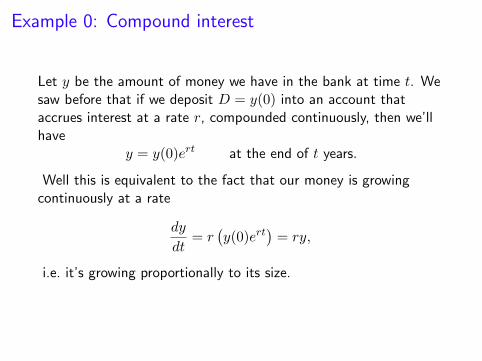
Let y be the amount of money we have in the bank at time t. Wesaw before that if we deposit D = y(0) into an account thataccrues interest at a rate r, compounded continuously, then we’llhave
y = y(0)ert at the end of t years.
Well this is equivalent to the fact that our money is growingcontinuously at a rate
dy
dt= r
(y(0)ert
)= ry,
i.e. it’s growing proportionally to its size.So continuouslycompounded interest was a natural growth problem.

Example 0: Compound interest
Let y be the amount of money we have in the bank at time t. Wesaw before that if we deposit D = y(0) into an account thataccrues interest at a rate r, compounded continuously, then we’llhave
y = y(0)ert at the end of t years.
Well this is equivalent to the fact that our money is growingcontinuously at a rate
dy
dt= r
(y(0)ert
)= ry,
i.e. it’s growing proportionally to its size.So continuouslycompounded interest was a natural growth problem.
Example 0: Compound interest
Let y be the amount of money we have in the bank at time t. Wesaw before that if we deposit D = y(0) into an account thataccrues interest at a rate r, compounded continuously, then we’llhave
y = y(0)ert at the end of t years.
Well this is equivalent to the fact that our money is growingcontinuously at a rate
dy
dt= r
(y(0)ert
)= ry,
i.e. it’s growing proportionally to its size.
So continuouslycompounded interest was a natural growth problem.

Example 0: Compound interest
Let y be the amount of money we have in the bank at time t. Wesaw before that if we deposit D = y(0) into an account thataccrues interest at a rate r, compounded continuously, then we’llhave
y = y(0)ert at the end of t years.
Well this is equivalent to the fact that our money is growingcontinuously at a rate
dy
dt= r
(y(0)ert
)= ry,
i.e. it’s growing proportionally to its size.So continuouslycompounded interest was a natural growth problem.
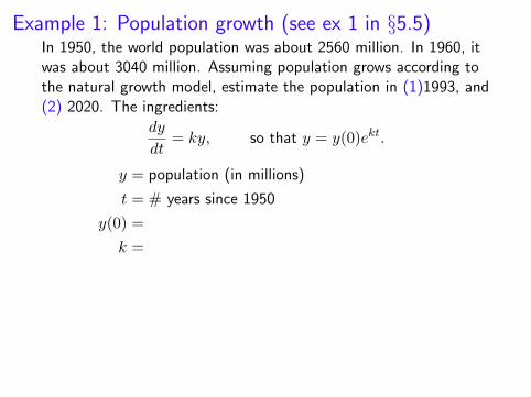
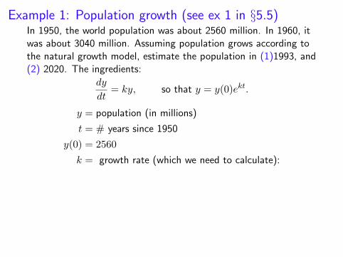
Example 1: Population growth (see ex 1 in §5.5)In 1950, the world population was about 2560 million. In 1960, itwas about 3040 million. Assuming population grows according tothe natural growth model, estimate the population in (1)1993, and(2) 2020.
The ingredients:
dy
dt= ky, so that y = y(0)ekt.
y =
population (in millions)
t =
# years since 1950
y(0) =
2560
k =
growth rate (which we need to calculate):
Use the other data point:
3040 = y(10) = 2560ek(10) so k =1
10ln
(3040
2560
)≈ .0172.
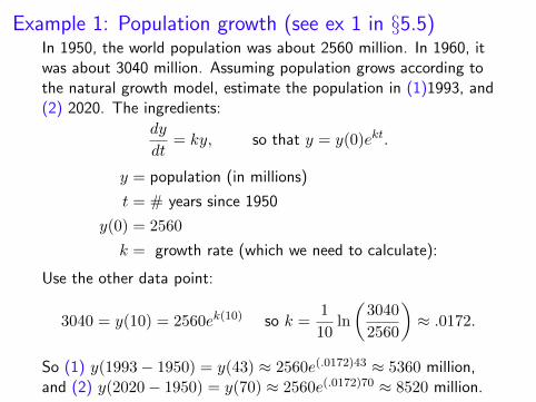
So (1) y(1993− 1950) = y(43) ≈ 2560e(.0172)43 ≈ 5360 million,and (2) y(2020− 1950) = y(70) ≈ 2560e(.0172)70 ≈ 8520 million.

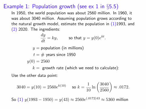
Example 1: Population growth (see ex 1 in §5.5)In 1950, the world population was about 2560 million. In 1960, itwas about 3040 million. Assuming population grows according tothe natural growth model, estimate the population in (1)1993, and(2) 2020. The ingredients:
dy
dt= ky, so that y = y(0)ekt.
y =
population (in millions)
t =
# years since 1950
y(0) =
2560
k =
growth rate (which we need to calculate):
Use the other data point:
3040 = y(10) = 2560ek(10) so k =1
10ln
(3040
2560
)≈ .0172.
So (1) y(1993− 1950) = y(43) ≈ 2560e(.0172)43 ≈ 5360 million,and (2) y(2020− 1950) = y(70) ≈ 2560e(.0172)70 ≈ 8520 million.

Example 1: Population growth (see ex 1 in §5.5)In 1950, the world population was about 2560 million. In 1960, itwas about 3040 million. Assuming population grows according tothe natural growth model, estimate the population in (1)1993, and(2) 2020. The ingredients:
dy
dt= ky, so that y = y(0)ekt.
y = population (in millions)
t =
# years since 1950
y(0) =
2560
k =
growth rate (which we need to calculate):
Use the other data point:
3040 = y(10) = 2560ek(10) so k =1
10ln
(3040
2560
)≈ .0172.
So (1) y(1993− 1950) = y(43) ≈ 2560e(.0172)43 ≈ 5360 million,and (2) y(2020− 1950) = y(70) ≈ 2560e(.0172)70 ≈ 8520 million.
Example 1: Population growth (see ex 1 in §5.5)In 1950, the world population was about 2560 million. In 1960, itwas about 3040 million. Assuming population grows according tothe natural growth model, estimate the population in (1)1993, and(2) 2020. The ingredients:
dy
dt= ky, so that y = y(0)ekt.
y = population (in millions)
t = # years since 1950
y(0) =
2560
k =
growth rate (which we need to calculate):
Use the other data point:
3040 = y(10) = 2560ek(10) so k =1
10ln
(3040
2560
)≈ .0172.
So (1) y(1993− 1950) = y(43) ≈ 2560e(.0172)43 ≈ 5360 million,and (2) y(2020− 1950) = y(70) ≈ 2560e(.0172)70 ≈ 8520 million.
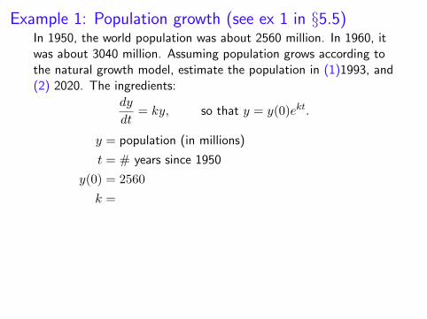
Example 1: Population growth (see ex 1 in §5.5)In 1950, the world population was about 2560 million. In 1960, itwas about 3040 million. Assuming population grows according tothe natural growth model, estimate the population in (1)1993, and(2) 2020. The ingredients:
dy
dt= ky, so that y = y(0)ekt.
y = population (in millions)
t = # years since 1950
y(0) = 2560
k =
growth rate (which we need to calculate):
Use the other data point:
3040 = y(10) = 2560ek(10) so k =1
10ln
(3040
2560
)≈ .0172.
So (1) y(1993− 1950) = y(43) ≈ 2560e(.0172)43 ≈ 5360 million,and (2) y(2020− 1950) = y(70) ≈ 2560e(.0172)70 ≈ 8520 million.
Example 1: Population growth (see ex 1 in §5.5)In 1950, the world population was about 2560 million. In 1960, itwas about 3040 million. Assuming population grows according tothe natural growth model, estimate the population in (1)1993, and(2) 2020. The ingredients:
dy
dt= ky, so that y = y(0)ekt.
y = population (in millions)
t = # years since 1950
y(0) = 2560
k = growth rate (which we need to calculate):
Use the other data point:
3040 = y(10) = 2560ek(10) so k =1
10ln
(3040
2560
)≈ .0172.
So (1) y(1993− 1950) = y(43) ≈ 2560e(.0172)43 ≈ 5360 million,and (2) y(2020− 1950) = y(70) ≈ 2560e(.0172)70 ≈ 8520 million.

Example 1: Population growth (see ex 1 in §5.5)In 1950, the world population was about 2560 million. In 1960, itwas about 3040 million. Assuming population grows according tothe natural growth model, estimate the population in (1)1993, and(2) 2020. The ingredients:
dy
dt= ky, so that y = y(0)ekt.
y = population (in millions)
t = # years since 1950
y(0) = 2560
k = growth rate (which we need to calculate):
Use the other data point:
3040 = y(10) = 2560ek(10)
so k =1
10ln
(3040
2560
)≈ .0172.
So (1) y(1993− 1950) = y(43) ≈ 2560e(.0172)43 ≈ 5360 million,and (2) y(2020− 1950) = y(70) ≈ 2560e(.0172)70 ≈ 8520 million.

Example 1: Population growth (see ex 1 in §5.5)In 1950, the world population was about 2560 million. In 1960, itwas about 3040 million. Assuming population grows according tothe natural growth model, estimate the population in (1)1993, and(2) 2020. The ingredients:
dy
dt= ky, so that y = y(0)ekt.
y = population (in millions)
t = # years since 1950
y(0) = 2560
k = growth rate (which we need to calculate):
Use the other data point:
3040 = y(10) = 2560ek(10) so k =1
10ln
(3040
2560
)≈ .0172.
So (1) y(1993− 1950) = y(43) ≈ 2560e(.0172)43 ≈ 5360 million,and (2) y(2020− 1950) = y(70) ≈ 2560e(.0172)70 ≈ 8520 million.
Example 1: Population growth (see ex 1 in §5.5)In 1950, the world population was about 2560 million. In 1960, itwas about 3040 million. Assuming population grows according tothe natural growth model, estimate the population in (1)1993, and(2) 2020. The ingredients:
dy
dt= ky, so that y = y(0)ekt.
y = population (in millions)
t = # years since 1950
y(0) = 2560
k = growth rate (which we need to calculate):
Use the other data point:
3040 = y(10) = 2560ek(10) so k =1
10ln
(3040
2560
)≈ .0172.
So (1) y(1993− 1950) = y(43) ≈ 2560e(.0172)43 ≈ 5360 million
,and (2) y(2020− 1950) = y(70) ≈ 2560e(.0172)70 ≈ 8520 million.
Example 1: Population growth (see ex 1 in §5.5)In 1950, the world population was about 2560 million. In 1960, itwas about 3040 million. Assuming population grows according tothe natural growth model, estimate the population in (1)1993, and(2) 2020. The ingredients:
dy
dt= ky, so that y = y(0)ekt.
y = population (in millions)
t = # years since 1950
y(0) = 2560
k = growth rate (which we need to calculate):
Use the other data point:
3040 = y(10) = 2560ek(10) so k =1
10ln
(3040
2560
)≈ .0172.
So (1) y(1993− 1950) = y(43) ≈ 2560e(.0172)43 ≈ 5360 million,and (2) y(2020− 1950) = y(70) ≈ 2560e(.0172)70 ≈ 8520 million.
Example 2: Radioactive decay (see ex 2 in §5.5)The half-life of a radioactive substance is the amount of time thatit takes for the substance to decay to half its original amount.
Inother words, if
y = mass of substance at time t, m0 = y(0)
and T = half-life of substance, then y(T ) = 12m0. (∗)
You try: The half-life of radium-226 is 1590 years. Assumeradium-226 decays according to the law of natural decay, i.e.dydt = ky so that y = y(0)ekt (∗∗), and suppose you start with100mg of the substance.
1. What are T and y(0)? What are the units on y and t?2. You have two data points — one comes from t = 0 that tells
you y(0); the other comes from y(T ) = 12y(0). Use the equ’ns
(∗) and (∗∗) to set up an equ’n where the only variable is k.3. Solve for k.4. Estimate the mass remaining after 1000 years.5. How long will it take for the mass to be reduced to 30 mg?

Example 2: Radioactive decay (see ex 2 in §5.5)The half-life of a radioactive substance is the amount of time thatit takes for the substance to decay to half its original amount. Inother words, if
y = mass of substance at time t, m0 = y(0)
and T = half-life of substance, then y(T ) = 12m0. (∗)
You try: The half-life of radium-226 is 1590 years. Assumeradium-226 decays according to the law of natural decay, i.e.dydt = ky so that y = y(0)ekt (∗∗), and suppose you start with100mg of the substance.
1. What are T and y(0)? What are the units on y and t?2. You have two data points — one comes from t = 0 that tells
you y(0); the other comes from y(T ) = 12y(0). Use the equ’ns
(∗) and (∗∗) to set up an equ’n where the only variable is k.3. Solve for k.4. Estimate the mass remaining after 1000 years.5. How long will it take for the mass to be reduced to 30 mg?
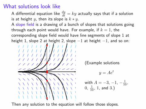
What solutions look likeA differential equation like dy
dt = ky actually says that if a solutionis at height y, then its slope is k ∗ y.
A slope field is a drawing of a bunch of slopes that solutions goingthrough each point would have. For example, if k = 1, thecorresponding slope field would have line segments of slope 1 atheight 1, slope 2 at height 2, slope −1 at height −1, and so on:
(Example solutions
y = Aet
with A = −3, −1, − 110 ,
0, 110 , 1, and 3.)
Then any solution to the equation will follow those slopes.
What solutions look likeA differential equation like dy
dt = ky actually says that if a solutionis at height y, then its slope is k ∗ y.A slope field is a drawing of a bunch of slopes that solutions goingthrough each point would have.
For example, if k = 1, thecorresponding slope field would have line segments of slope 1 atheight 1, slope 2 at height 2, slope −1 at height −1, and so on:
(Example solutions
y = Aet
with A = −3, −1, − 110 ,
0, 110 , 1, and 3.)
Then any solution to the equation will follow those slopes.
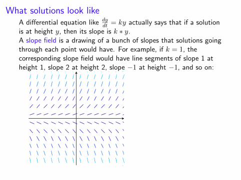
What solutions look likeA differential equation like dy
dt = ky actually says that if a solutionis at height y, then its slope is k ∗ y.A slope field is a drawing of a bunch of slopes that solutions goingthrough each point would have. For example, if k = 1, thecorresponding slope field would have line segments of slope 1 atheight 1, slope 2 at height 2, slope −1 at height −1, and so on:
(Example solutions
y = Aet
with A = −3, −1, − 110 ,
0, 110 , 1, and 3.)
Then any solution to the equation will follow those slopes.
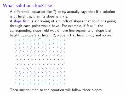
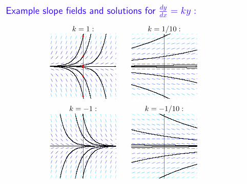
Example slope fields and solutions for dydx = ky :
k = 1 : k = 1/10 :
k = −1 : k = −1/10 :
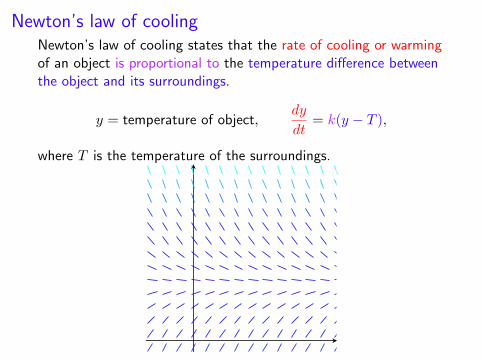
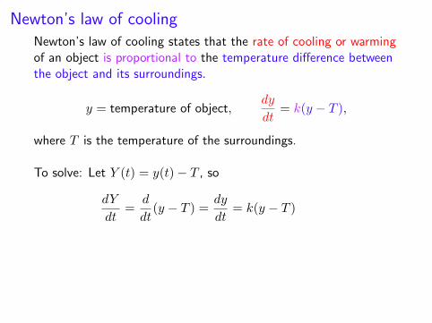
Newton’s law of coolingNewton’s law of cooling states that the rate of cooling or warmingof an object is proportional to the temperature difference betweenthe object and its surroundings.
y = temperature of object,dy
dt= k(y − T ),
where T is the temperature of the surroundings.
Newton’s law of coolingNewton’s law of cooling states that the rate of cooling or warmingof an object is proportional to the temperature difference betweenthe object and its surroundings.
y = temperature of object,dy
dt= k(y − T ),
where T is the temperature of the surroundings.
Newton’s law of coolingNewton’s law of cooling states that the rate of cooling or warmingof an object is proportional to the temperature difference betweenthe object and its surroundings.
y = temperature of object,dy
dt= k(y − T ),
where T is the temperature of the surroundings.
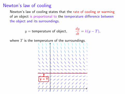
Newton’s law of coolingNewton’s law of cooling states that the rate of cooling or warmingof an object is proportional to the temperature difference betweenthe object and its surroundings.
y = temperature of object,dy
dt= k(y − T ),
where T is the temperature of the surroundings.
y = T
Newton’s law of coolingNewton’s law of cooling states that the rate of cooling or warmingof an object is proportional to the temperature difference betweenthe object and its surroundings.
y = temperature of object,dy
dt= k(y − T ),
where T is the temperature of the surroundings.
y = T
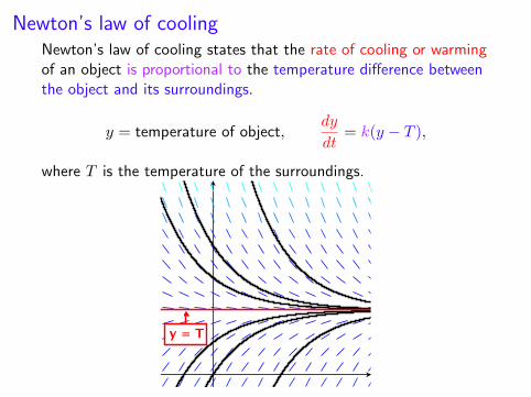
Newton’s law of coolingNewton’s law of cooling states that the rate of cooling or warmingof an object is proportional to the temperature difference betweenthe object and its surroundings.
y = temperature of object,dy
dt= k(y − T ),
where T is the temperature of the surroundings.
To solve: Let Y (t) = y(t)− T ,
so
dY
dt=
d
dt(y − T ) =
dy
dt= k(y − T ) = kY.
Thus Y (t) = Y (0)ekt. Substituting back, we have
y − T = (y(0)− T )ekt, i.e., y(t) = (y(0)− T )ekt + T .
Note, if y(0) = T , this is the constant function y = T .

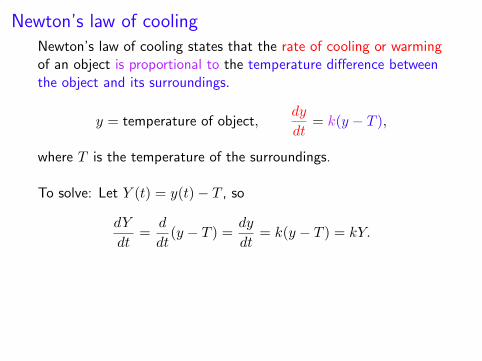
Newton’s law of coolingNewton’s law of cooling states that the rate of cooling or warmingof an object is proportional to the temperature difference betweenthe object and its surroundings.
y = temperature of object,dy
dt= k(y − T ),
where T is the temperature of the surroundings.
To solve: Let Y (t) = y(t)− T , so
dY
dt=
d
dt(y − T ) =
dy
dt
= k(y − T ) = kY.
Thus Y (t) = Y (0)ekt. Substituting back, we have
y − T = (y(0)− T )ekt, i.e., y(t) = (y(0)− T )ekt + T .
Note, if y(0) = T , this is the constant function y = T .
Newton’s law of coolingNewton’s law of cooling states that the rate of cooling or warmingof an object is proportional to the temperature difference betweenthe object and its surroundings.
y = temperature of object,dy
dt= k(y − T ),
where T is the temperature of the surroundings.
To solve: Let Y (t) = y(t)− T , so
dY
dt=
d
dt(y − T ) =
dy
dt= k(y − T )
= kY.
Thus Y (t) = Y (0)ekt. Substituting back, we have
y − T = (y(0)− T )ekt, i.e., y(t) = (y(0)− T )ekt + T .
Note, if y(0) = T , this is the constant function y = T .
Newton’s law of coolingNewton’s law of cooling states that the rate of cooling or warmingof an object is proportional to the temperature difference betweenthe object and its surroundings.
y = temperature of object,dy
dt= k(y − T ),
where T is the temperature of the surroundings.
To solve: Let Y (t) = y(t)− T , so
dY
dt=
d
dt(y − T ) =
dy
dt= k(y − T ) = kY.
Thus Y (t) = Y (0)ekt. Substituting back, we have
y − T = (y(0)− T )ekt, i.e., y(t) = (y(0)− T )ekt + T .
Note, if y(0) = T , this is the constant function y = T .
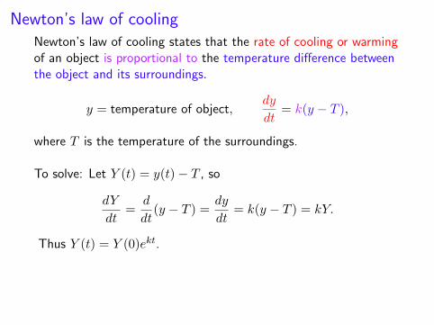
Newton’s law of coolingNewton’s law of cooling states that the rate of cooling or warmingof an object is proportional to the temperature difference betweenthe object and its surroundings.
y = temperature of object,dy
dt= k(y − T ),
where T is the temperature of the surroundings.
To solve: Let Y (t) = y(t)− T , so
dY
dt=
d
dt(y − T ) =
dy
dt= k(y − T ) = kY.
Thus Y (t) = Y (0)ekt.
Substituting back, we have
y − T = (y(0)− T )ekt, i.e., y(t) = (y(0)− T )ekt + T .
Note, if y(0) = T , this is the constant function y = T .

Newton’s law of coolingNewton’s law of cooling states that the rate of cooling or warmingof an object is proportional to the temperature difference betweenthe object and its surroundings.
y = temperature of object,dy
dt= k(y − T ),
where T is the temperature of the surroundings.
To solve: Let Y (t) = y(t)− T , so
dY
dt=
d
dt(y − T ) =
dy
dt= k(y − T ) = kY.
Thus Y (t) = Y (0)ekt. Substituting back, we have
y − T = (y(0)− T )ekt,
i.e., y(t) = (y(0)− T )ekt + T .
Note, if y(0) = T , this is the constant function y = T .
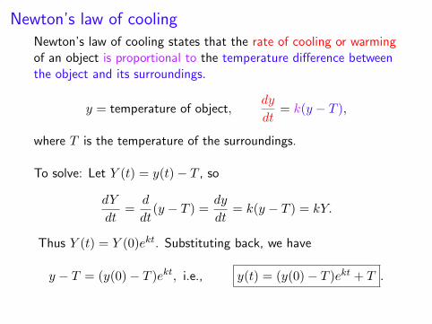
Newton’s law of coolingNewton’s law of cooling states that the rate of cooling or warmingof an object is proportional to the temperature difference betweenthe object and its surroundings.
y = temperature of object,dy
dt= k(y − T ),
where T is the temperature of the surroundings.
To solve: Let Y (t) = y(t)− T , so
dY
dt=
d
dt(y − T ) =
dy
dt= k(y − T ) = kY.
Thus Y (t) = Y (0)ekt. Substituting back, we have
y − T = (y(0)− T )ekt, i.e., y(t) = (y(0)− T )ekt + T .
Note, if y(0) = T , this is the constant function y = T .

Newton’s law of coolingNewton’s law of cooling states that the rate of cooling or warmingof an object is proportional to the temperature difference betweenthe object and its surroundings.
y = temperature of object,dy
dt= k(y − T ),
where T is the temperature of the surroundings.
To solve: Let Y (t) = y(t)− T , so
dY
dt=
d
dt(y − T ) =
dy
dt= k(y − T ) = kY.
Thus Y (t) = Y (0)ekt. Substituting back, we have
y − T = (y(0)− T )ekt, i.e., y(t) = (y(0)− T )ekt + T .
Note, if y(0) = T , this is the constant function y = T .

Related Documents