To the University of Wyoming: The members of the Committee approve the dissertation of Enrico Fabiano presented on April 7, 2017. Dr. Dimitri J. Mavriplis, Chairperson Dr. Craig C. Douglas, External Department Member Dr. Jonathan Naughton Dr. Jayanarayanan Sitaraman Dr. Giuseppe Quaranta, External Examiner, Politecnico Di Milano, Italy APPROVED: Dr. Carl Frick, Head, Department of Mechanical Engineering Robert Ettema, Dean, College of Engineering and Applied Science

Welcome message from author
This document is posted to help you gain knowledge. Please leave a comment to let me know what you think about it! Share it to your friends and learn new things together.
Transcript

To the University of Wyoming:The members of the Committee approve the dissertation of Enrico Fabiano presented on
April 7, 2017.
Dr. Dimitri J. Mavriplis, Chairperson
Dr. Craig C. Douglas, External Department Member
Dr. Jonathan Naughton
Dr. Jayanarayanan Sitaraman
Dr. Giuseppe Quaranta, External Examiner, Politecnico Di Milano, Italy
APPROVED:
Dr. Carl Frick, Head, Department of Mechanical Engineering
Robert Ettema, Dean, College of Engineering and Applied Science

Fabiano, Enrico, Multidisciplinary Adjoint-based Design Optimization Techniques for HelicopterRotors, Ph.D., Department of Mechanical Engineering, May, 2017.
Helicopter rotor design optimization is a challenging task due to the multidisciplinary nature
of rotorcraft design: the helicopter operates in a highly unsteady aerodynamic environment, highly
flexible, slender rotor blades highlight the importance of blade aeroelasticity, while the ever more
stringent noise requirements that the helicopter must satisfy underlines the need to include aeroa-
coustic considerations early in the design process.
Such a large scale problem can be efficiently solved with the use of gradient-based optimization
methods. In gradient based optimization, the gradient of the objective function with respect to the
design variables is needed to determine a search direction. The objective function’s gradient can be
computed either with the finite difference approach, the tangent or forward linearization approach
and the adjoint or reverse approach. The finite difference approach is easy to implement but its cost
scales with the number of design variables and can be affected by the choice of the step size used
in the differentiation. The tangent or forward approach computes the exact gradient vector of the
objective function by exact differentiation of the computational code, however its cost still scales
linearly with the number of design variables. On the other hand, the adjoint or reverse approach
computes the sensitivity vector with respect to a potentially infinite number of design variables at
a cost essentially independent of the design variables, making the adjoint technique the only vi-
able approach when the number of design variables is large. Hence, it is the adjoint approach that
makes gradient based optimization techniques competitive for large scale problems characterized
by a large number of design parameters, such as the current helicopter design problem.
The focus of this work is the development of a high-fidelity multidisciplinary adjoint technique that
encompasses the three disciplines of aerodynamics, structural mechanics and aeroacoustics for ro-
torcraft problems. Upon successful implementation and verification, the multidisciplinary adjoint
method is applied to the problem of noise minimization of a flexible rotor in trimmed forward
flight with no performance penalty. Optimization results highlight the potential of high-fidelity
multidisciplinary design optimization for helicopter rotors.
1

MULTIDISCIPLINARY ADJOINT-BASED DESIGNOPTIMIZATION TECHNIQUES FOR HELICOPTER
ROTORS
by
Enrico Fabiano
A dissertation submitted to theUniversity of Wyoming
in partial fulfillment of the requirementsfor the degree of
DOCTOR OF PHILOSOPHYin
MECHANICAL ENGINEERING
Laramie, WyomingMay 2017

Copyright c© 2017
by
Enrico Fabiano
ii

Faster and Higher
iii

Contents
List of Figures vi
List of Tables ix
Acknowledgments x
Chapter 1 Introduction 1
1.1 Helicopter Design: a Multidisciplinary Design Optimization Problem . . . . . . . 1
1.2 Helicopter Aeroacoustics . . . . . . . . . . . . . . . . . . . . . . . . . . . . . . . 3
1.3 Optimization Techniques and Their Application to Rotorcraft Design . . . . . . . . 4
1.4 Unique Aspects of the Current Work . . . . . . . . . . . . . . . . . . . . . . . . . 7
Chapter 2 Two Dimensional Aeroacoustic Problem 8
2.1 Aerodynamic Solver . . . . . . . . . . . . . . . . . . . . . . . . . . . . . . . . . 8
2.2 Airfoil Surface Parameterization and Mesh Deformation Algorithm . . . . . . . . 10
2.3 Two-dimensional Blade-Vortex Interaction Noise . . . . . . . . . . . . . . . . . . 12
2.4 Aeroacoustic Solver: the Two-dimensional FW-H Integration . . . . . . . . . . . . 14
2.5 Tangent and Adjoint Formulations for the Two-dimensional Aeroacoustic Problem 19
2.5.1 Sensitivity Analysis Formulation for Airfoil in Vortex Interaction . . . . . 20
2.5.2 Sensitivity Analysis for the FW-H Equation . . . . . . . . . . . . . . . . . 26
Chapter 3 Three Dimensional Aeroacoustic Problem for Helicopter Rotors 30
3.1 Aerodynamic Solver . . . . . . . . . . . . . . . . . . . . . . . . . . . . . . . . . 30
3.2 Structural Dynamics Solver . . . . . . . . . . . . . . . . . . . . . . . . . . . . . . 31
iv

3.2.1 Fluid-structure Interface . . . . . . . . . . . . . . . . . . . . . . . . . . . 33
3.3 Prescribed Blade Motion . . . . . . . . . . . . . . . . . . . . . . . . . . . . . . . 33
3.4 Geometry Parameterization Facility . . . . . . . . . . . . . . . . . . . . . . . . . 34
3.5 Mesh Deformation Capability . . . . . . . . . . . . . . . . . . . . . . . . . . . . 35
3.6 Aeroacoustic Solver: the Three-dimensional FW-H Integration . . . . . . . . . . . 35
3.7 Fully Coupled Multidisciplinary Analysis Problem . . . . . . . . . . . . . . . . . 40
3.8 Fully Coupled Multidisciplinary Tangent and Adjoint Problems . . . . . . . . . . . 42
3.8.1 Sensitivity Formulation for the Integral FW-H Equation . . . . . . . . . . 48
Chapter 4 Optimization Results 53
4.1 Two-dimensional Optimization Results . . . . . . . . . . . . . . . . . . . . . . . . 53
4.1.1 L-BFGS-B Optimization . . . . . . . . . . . . . . . . . . . . . . . . . . . 55
4.1.2 Sequential Quadratic Programming Optimization . . . . . . . . . . . . . . 59
4.2 Three-Dimensional Optimization Results . . . . . . . . . . . . . . . . . . . . . . 59
4.2.1 Rigid HART-II Rotor . . . . . . . . . . . . . . . . . . . . . . . . . . . . . 65
4.2.2 Flexible HART-II Rotor . . . . . . . . . . . . . . . . . . . . . . . . . . . 82
Chapter 5 Conclusions and Future Work 99
References 103
v

List of Figures
2.1 Schematic of the CST geometry parameterization technique for the NACA 0012
airfoil represented with Bernstein polynomials of order 8 . . . . . . . . . . . . . . 11
2.2 Initialization of the isentropic vortex in the steady state flowfield computed around
the NACA-0012 airfoil. . . . . . . . . . . . . . . . . . . . . . . . . . . . . . . . . 13
2.3 Residual convergence for the first three timestep of the unsteady CFD solution . . . 13
2.4 CFD mesh and approximate location of the FW-H integration surface . . . . . . . 16
2.5 Validation of the two-dimensional acoustic integration for the monopole in uniform
flow test case [48] . . . . . . . . . . . . . . . . . . . . . . . . . . . . . . . . . . . 18
2.6 Schematic of the scattering by an edge from Rumpfkeil [51] . . . . . . . . . . . . 19
2.7 Validation of the acoustic solver for the scattering of sound by an edge [50] . . . . 20
2.8 Residual convergence for the flow adjoint problem at a generic timestep and the
final mesh adjoint problem . . . . . . . . . . . . . . . . . . . . . . . . . . . . . . 24
2.9 Comparison of FW-H propagated and CFD computed acoustic pressure sensitivity
at different observer locations highlighting the detrimental effect that numerical
dissipation has on the computed acoustic pressure sensitivity as the observer is
moved to the far field. . . . . . . . . . . . . . . . . . . . . . . . . . . . . . . . . . 28
3.1 Beam element with flap, lag, torsional and axial (total 15) degrees of freedom. . . . 32
3.2 Acoustic integration surface and observer location: the observer is stationary in the
plane of the rotor two radii from the rotor hub at ψ = 180 deg. . . . . . . . . . . . 36
3.3 Validation of the current FW-H implementation over an extended (a) and the opti-
mization (b) time window . . . . . . . . . . . . . . . . . . . . . . . . . . . . . . . 41
vi

3.4 Acoustic pressure at the observer for the baseline rigid and flexible HART-II rotor. 43
3.5 Comparison between the rigid and the flexible HART-II rotor. . . . . . . . . . . . . 43
3.6 Flow of information for analysis, tangent and adjoint solution processes at every
timestep. . . . . . . . . . . . . . . . . . . . . . . . . . . . . . . . . . . . . . . . . 49
3.7 Complex step verification of the tangent acoustic pressure time history sensitivity . 52
4.1 Baseline, acoustically optimized (ω = 1) and aeroacoustically optimized (ω = 0.1)
airfoils . . . . . . . . . . . . . . . . . . . . . . . . . . . . . . . . . . . . . . . . . 56
4.2 Lift time histories for the baseline and the optimized airfoil highlithing the impor-
tance of the aerodynamic penalty term . . . . . . . . . . . . . . . . . . . . . . . . 57
4.3 Convergence of the L-BFGS-B ω = 0.1 optimization . . . . . . . . . . . . . . . . 58
4.4 Baseline, L-BFGSB-B (ω = 0.1) and SQP optimized airfoils. . . . . . . . . . . . . 60
4.5 Baseline, L-BFGSB-B (ω = 0.1) and SQP lift time histories. . . . . . . . . . . . . 60
4.6 Convergence of the Sequential Quadratic Programming optimization for the NACA
0012 airfoil . . . . . . . . . . . . . . . . . . . . . . . . . . . . . . . . . . . . . . 61
4.7 Convergence of the rigid trim optimization problem . . . . . . . . . . . . . . . . . 66
4.8 Thrust and moments time histories for the trimmed baseline HART-II rigid rotor . . 68
4.9 Convergence of the aeroacoustic optimization problem for the rigid HART-II rotor . 70
4.10 Thrust and moment time histories for the aeroacoustically optimized HART-II rigid
rotor . . . . . . . . . . . . . . . . . . . . . . . . . . . . . . . . . . . . . . . . . . 72
4.11 Thickness, loading and total acoustic pressures at the observer for the aeroacousti-
cally optimized rigid rotor . . . . . . . . . . . . . . . . . . . . . . . . . . . . . . 73
4.12 Baseline and optimized airfoil shapes for the aeroacoustically optimized rigid rotor 73
4.13 Baseline and optimized torque time histories for the aeroacoustically optimized
rigid rotor showing the performance penalty paid to minimize the acoustic signature. 74
4.14 Convergence of the torque-constrained aeroacoustic optimization problem . . . . . 76
4.15 Thrust and moment time histories for baseline and the torque-constrained aeroa-
coustically optimized trimmed HART-II rigid rotor . . . . . . . . . . . . . . . . . 78
4.16 Baseline and optimized torque time histories for the torque-constrained aeroacous-
tically optimized rigid rotor. . . . . . . . . . . . . . . . . . . . . . . . . . . . . . 79
vii

4.17 Thickness, loading and total acoustic pressures at the observer for the torque -
constrained aeroacoustically optimized rigid rotor . . . . . . . . . . . . . . . . . . 80
4.18 Torque-constrained aeroacoustically optimized airfoil shapes . . . . . . . . . . . . 80
4.19 Directivity study for the baseline and optimized rigid rotor geometries . . . . . . . 81
4.20 Convergence of the trim optimization problem for the flexible HART-II rotor . . . 83
4.21 Thrust and moments time histories for the baseline HART-II flexible rotor . . . . . 84
4.22 Convergence of the flexible aeroacoustic optimization problem . . . . . . . . . . . 86
4.23 Thrust and moments time histories for the baseline and optimized flexible HART-II
rotors . . . . . . . . . . . . . . . . . . . . . . . . . . . . . . . . . . . . . . . . . 87
4.24 Thickness, loading and total acoustic pressures at the observer for the baseline
(red) and the aeroacoustically optimized (green) flexible rotors . . . . . . . . . . . 87
4.25 Baseline (red) and optimized (green) airfoil shapes for the aeroacoustically opti-
mized flexible rotors . . . . . . . . . . . . . . . . . . . . . . . . . . . . . . . . . 88
4.26 Torque time history for the baseline and aeroacoustically optimized flexible rotors
showing the performance penalty paid to minimize the acoustic signature. . . . . . 88
4.27 Convergence of the acoustically constrained torque optimization of the flexible
HART-II rotor . . . . . . . . . . . . . . . . . . . . . . . . . . . . . . . . . . . . . 91
4.28 Thrust and moments time histories for the baseline, the aeroacoustic optimized and
the acoustically constrained torque optimized flexible rotors . . . . . . . . . . . . 92
4.29 Torque time histories for the baseline, the aeroacoustic optimized and the acousti-
cally constrained torque optimized flexible rotors . . . . . . . . . . . . . . . . . . 93
4.30 Thickness, loading and total acoustic pressures at the observer for the baseline
(red), the acoustically optimized (green) and the acoustically constrained torque
optimized (blue) flexible rotors. . . . . . . . . . . . . . . . . . . . . . . . . . . . 94
4.31 Acoustically constrained torque optimized blade shapes . . . . . . . . . . . . . . . 94
4.32 Directivity study for the baseline and optimized flexible geometries: radial distance
2R, different azimuthal locations . . . . . . . . . . . . . . . . . . . . . . . . . . . 95
4.33 Directivity study for the baseline and optimized flexible geometries: Azimuth ψ =
180 degs, different radial locations . . . . . . . . . . . . . . . . . . . . . . . . . . 96
viii

4.34 Thrust and moments time histories for the baseline, the aeroacoustic optimized and
the acoustically constrained torque optimized flexible rotors over 4 rotor revolutions 97
4.35 Thickness, loading and total acoustic pressures at the observer for the baseline and
the two optimized flexible rotors for the multiple revolutions case. . . . . . . . . . 97
4.36 Torque time histories for the baseline, the aeroacoustic optimized and the acousti-
cally constrained torque optimized flexible rotors over 4 rotor revolutions . . . . . 98
ix

List of Tables
2.1 Complex step validation of the 7th design sensitivity of the flow adjoint. . . . . . . 26
2.2 Finite difference validation of the 7th design sensitivity. . . . . . . . . . . . . . . 29
3.1 Comparison of HART-II Natural Frequencies [65] . . . . . . . . . . . . . . . . . . 33
3.2 Observer location for the acoustic objective function with respect to the rotor hub,
R being the rotor radius . . . . . . . . . . . . . . . . . . . . . . . . . . . . . . . . 40
3.3 Adjoint sensitivity verification for the p′RMS objective function w.r.t. the root twist
design variable. . . . . . . . . . . . . . . . . . . . . . . . . . . . . . . . . . . . . 52
3.4 Adjoint sensitivity verification for the p′RMS objective function w.r.t. the first cyclic
design variable. . . . . . . . . . . . . . . . . . . . . . . . . . . . . . . . . . . . . 52
4.1 Overall Sound Pressure Level (OSPL) values for different weights ω. . . . . . . . . 56
4.2 Operating condition for the HART-II rotor in trimmed forward flight . . . . . . . . 64
4.3 Twist, collective and cyclics values for the baseline and the aeroacoustically opti-
mized rigid rotors. All quantities in degrees . . . . . . . . . . . . . . . . . . . . . 68
4.4 Twist, collective and cyclics values for the baseline and the aeroacoustically opti-
mized rigid rotors. All quantities in degrees. . . . . . . . . . . . . . . . . . . . . . 82
4.5 Twist, collective and cyclics values for the baseline and the aeroacoustically opti-
mized flexible rotors. All quantities in degrees. . . . . . . . . . . . . . . . . . . . 86
4.6 Twist, collective and cyclics values for the baseline and the aeroacoustically opti-
mized flexible rotors. All quantities in degrees. . . . . . . . . . . . . . . . . . . . 89
x

Acknowledgments
The list of persons that I feel I should thank is way too long to be contained in one page. I am
thankful to all of you and I apologize to those that I won’t be able to mention here.
I want to dedicate this work to my parents for their constant and unconditional love: this would
have never been possible without you.
I am extremely grateful to my advisor, Dimitri Mavriplis, for teaching me the fundamentals of
CFD and guiding me during the past few years: he will always remain my ”boss”. I would also
like to thank the other members of my committee for their support during my time at the University
of Wyoming and for reading this dissertation.
All the persons that I have met in Laramie and at the ”lab” should also be mentioned here. I will
single out Karthik, Asitav, Lina, Renee, Ana and Bruce, but this list is far from being complete.
Mr. Giorgio Travostino deserves special mention: he introduced me to the world of aerodynamics
and CFD. Here is to many more dinners together.
Finally, I would like to acknowledge the Alfred Gessow Vertical Lift Research Center of Excel-
lence at the University of Maryland for funding this research.
ENRICO FABIANO
University of Wyoming
May 2017
xi

Chapter 1
Introduction
Helicopter rotor optimization is a challenging task due to the multidisciplinary nature of rotorcraft
design, the complex and intrinsically unsteady operating environment of the rotor and the poten-
tially large number of design variables. Such a large-scale problem can be efficiently solved with
the use of gradient-based optimization methods when the gradient of the optimization objective
function is computed with the adjoint approach. Hence, the goal of the work presented in this
thesis is the development of a high-fidelity multidisciplinary adjoint-based design optimization
capability for helicopter rotors that encompasses the three disciplines of aerodynamics, structural
mechanics and aeroacoustics.
1.1 Helicopter Design: a Multidisciplinary Design Optimiza-
tion Problem
The helicopter is an aircraft that uses two or more rotating wings to generate aerodynamic forces
in order to sustain controlled flight [1]. The rotors operate in a complex unsteady aerodynamic
environment characterized by vortical flow structures, wakes and, possibly, shock waves, and they
provide lift, propulsion and control forces to the aircraft. The aerodynamic forces are generated
by the relative motion between the rotors and the surrounding air even when the translational ve-
locity of the aircraft is zero. This provides the helicopter its most distinguished feature: the ability
to perform efficient hovering and vertical flights. However, large rotor diameters are needed to
1

achieve efficient vertical flight while high-aspect ratio blades guarantee the desired aerodynamic
efficiency. Hence, the structural design requirements that the rotor must satisfy to guarantee the
proper aerodynamic performance yield highly flexible blades whose aerostructural response needs
to be taken into account in the rotor design process. Furthermore, the propulsive forces necessary
for the helicopter to sustain translational flight are achieved by tilting the main rotor, resulting in
a lift imbalance between the advancing and retreating side of the blade: the advancing side is sub-
ject to higher velocity than the retreating side as a consequence of the combined translational and
rotational velocity of the rotor. This, however, generates pitching and rolling moments on the rotor
that need to be counteracted with a blade cyclic pitching motion to sustain trimmed level flight [1],
effectively coupling the aerodynamics and flight mechanics problem.
Finally, the ability to take off and land vertically (VTOL), and to maneuver in tightly confined
spaces makes the helicopter the perfect air vehicle to operate in urban environments leading to
very strict noise requirements. Hence, the aeroacoustic problem needs to be addressed early in the
design process and typically requires the detailed knowledge of the flowfield surrounding the rotor
and its aeroelastically deformed shape.
The tight interaction between all the disciplines involved in helicopter operations makes the heli-
copter design an intrinsically multidisciplinary design problem: the accurate computation of the
aerodynamic loads that the rotor must sustain is necessary to determine the correct structural de-
formation of the blades and the blade pitch controls necessary to sustain trimmed forward flight.
Once the blade shape, pitch controls and aerodynamic loads are computed, the correct acoustic
signature and aerodynamic performance can finally be determined.
Furthermore, the number of parameters that the designer can change to improve the rotorcraft per-
formance is potentially high, making the multidisciplinary design problem a large-scale design
optimization problem. To solve this multidisciplinary design problem the helicopter designer can
change a large number of design variables, typically consisting of airfoil shapes, structural proper-
ties and pitch control parameters, making the multidisciplinary design problem a large scale design
optimization problem. This large-scale multidisciplinary problem has traditionally been tackled
using lower fidelity models for each discipline involved, particularly aerodynamics and structural
mechanics, linked together in so-called comprehensive analysis codes, of which CAMRAD is the
2

perfect example [2]. Despite sacrificing accuracy, low fidelity models have seen widespread use in
the past because of the limited computational power available and the quick turnaround time they
offered in evaluating a significant number of design configurations. More recently, efforts have
been aimed at introducing higher-fidelity models earlier in the design process, particularly for the
aerodynamics. Notable examples of these efforts are the U.S. Army HELIOS computer code [3]
and its french counterpart [4]. A new high-fidelity multidisciplinary design analysis and optimiza-
tion tool for the design of helicopter rotors in trimmed forward flight is presented in this work. This
new tool encompasses the three disciplines of aerodynamics, structural mechanics and aeroacous-
tics and it is applied to the redesign of the flexible HART-II rotor [5] to improve its aeroacoustic
and aerodynamic performance.
1.2 Helicopter Aeroacoustics
As the importance of reducing detection distance and helicopter noise signature increases for both
commercial and military applications [1, 6], rotorcraft aeroacoustics takes on a leading role in the
helicopter design process. Hence, a significant portion of this work will focus on including a noise
prediction capability in the multidisciplinary design optimization process. Rotorcraft aeroacous-
tics have been widely studied in the past [7] and are now fairly well understood. Both discrete
frequencies and broadband aerodynamic noise is generated through different noise mechanisms.
Discrete frequency noise is deterministic in nature and divided into different components such as
thickness and loading noise, blade vortex interaction noise and high speed impulsive noise. Broad-
band noise is typically non-deterministic and associated with the turbulent flowfield surrounding
the rotor. In this work only deterministic noise is considered.
To minimize the rotor noise signature, both passive and active noise minimiztion techniques have
been investigated in the past. Common passive noise minimization techniques consist of a judi-
cious selection of rotor blade configurations, airfoils, planform and tip shapes [6]. Active control
techniques such as Higher Harmonic Control (HHC), Individual Blade Control (IBC) and active
flap configurations have also been investigated [6–8]. While these methods mainly rely on expen-
sive wind tunnel experiments and on the experience of the aircraft designer, few attempts have
3

been made at exploiting numerical shape optimization techniques in the context of noise reduction
for rotating aerodynamic surfaces: Chae et al. [9] optimized the acoustic signature of a hover-
ing rotor targeting mainly high speed impulsive (HSI) noise, while Marinus et al. [10] performed a
multiobjective, multidisciplinary optimization of transonic propeller blades targeting aerodynamic,
aeroelastic and aeroacoustic performance.
From a computational point of view the acoustic problem corresponds to propagating the acoustic
waves generated by the moving rotor to an observer possibly far away from the rotor itself. One
obvious approach to the solution of the acoustic problem is to resolve the acoustic waves to the
observer. Despite reasonable success for near and mid-field observers [11, 12], the computational
cost of this approach for far-field acoustic problems is still too high even for the current generation
of supercomputers. A more viable and widely employed solution to the aeroacoustic problem is
the use of Lightill’s acoustic analogy. This is a hybrid approach in which a nearbody aerodynamic
solver provides the flow information to an integral acoustic formulation that propagates the acous-
tic waves to the far-field observer. In this work the acoustic analogy approach has been followed
by implementing a Ffowcs-Williams Hawkings (FWH) acoustic integration procedure [13, 14] to
determine the rotor’s noise signature. After validation of the new FWH implementation, an adjoint
sensitivity approach has been developed to perform the noise minimization of the flexible HART-II
rotor in trimmed forward flight.
1.3 Optimization Techniques and Their Application to Rotor-
craft Design
Numerical shape optimization techniques in conjunction with Computational Fluid Dynamics
(CFD) have become a common tool in the aircraft design industry [15], and numerical shape opti-
mization for aeroacoustic and aerodynamic performance is the focus of this work.
Numerical optimization algorithms are divided in two broad categories: global or evolutionary
methods and local or gradient based methods. Evolutionary methods are easy to apply to rotorcraft
design problem as they only require the value of the objective function at the design point cur-
rently evaluated and, in case of a multimodal design space, they converge to the global optimum.
4

However, they require a significant number of function evaluations rendering their applications to
design problems involving high-fidelity, computationally-intensive models impractical. The cost
of evolutionary algorithms can be reduced when these are used in conjunction with metamod-
eling techniques [16], e.g. response surfaces, kriging methods and neural networks. However,
metamodeling techniques are not well suited for optimization problems characterized by a large
number of design variables [16]. Despite these limitations, evolutionary algorithms augmented
with metamodeling techniques have been used in the context of airfoil optimization [17], propeller
blade optimization [10, 18] and rotorcraft design [9]. Jones et al. [17] used a genetic algorithm
in conjunction with an aerodynamic low-fidelity model to perform the multidisciplinary optimiza-
tion of rotor blade shapes with up to 20 design parameters. Despite the quick turn-around time of
the low-fidelity aerodynamic model, the authors had to reduce the computational burden by using
a Message-Passing Interface to distribute the numerous function evaluations over multiple cores.
Marinus et al. [10, 18] performed high-fidelity design optimization of a propeller blade for aero-
dynamic, aeroelastic and aeroacoustic performance with up to 30 design variables. Finally, Chae
et al. [9] performed a high-fidelity design optimization of a hovering helicopter rotor to improve
its high speed impulsive noise with up to 19 design variables. Despite their success, these appli-
cations reveal the high computaional cost of evolutionary algorithm even when they are applied to
small-scale design optimization problems.
While a judicious selection of the design space parameterization is fundametnal for a successful
optimization [19], limiting the number of design variable can have a detrimental effect on the
overall optimization process and on the success of the rotorcraft design program. Furthermore, as
more and more disciplines are included in the design optimization process, the number of design
variables is expected to increase, exacerbating the issues associated with evolutionary algorithms.
Hence, evolutionary methods are not well suited for large-scale multidisciplinary rotorcraft de-
sign problems. Contrary to evolutionary algorithms, gradient-based optimization methods require
vastly fewer function evaluations provided that an efficient method for the computation of the
gradient of the optimization objective function exists. This makes gradient-based optimization al-
gorithms the only feasible alternative for the solution of large-scale, high-fidelity multidisciplinary
design optimization problems.
5

Gradient-based methods have been the first methods to be applied to rotorcraft problems [20, 21].
Whether in their unconstrained or constrained form, they use the gradient of the objective and
of the constraints of the design problem to find a direction to the nearest saddle point of the La-
grangian function associated with the optimization problem [22]. If the cost of computing the
objective function’s gradient is independent of the number of design variables, the performance of
gradient-based methods is relatively independent of the number of design parameters.
Different methods exist for computing the gradient of an objective function [22]. Traditionally the
finite-difference method has been used as it is extremely easy to implement. It is also an expensive
method as, in the best case, it requires N + 1 function evaluations, N being the number of design
parameters. Furthermore, the accuracy of the method depends on the step size used for differen-
tiation. Exact hand-differentiation of the computer code in forward or tangent mode removes the
accuracy issue associated with the step size, but its cost still scales linearly with the number of
design variables. However, exact hand-differentiation in reverse or adjoint mode removes the cost
issue as its computational cost is independent of the number of design variables. Adjoint sensi-
tivity formulations are a common tool in the context of CFD-based shape optimization since they
allow the computation of the sensitivities of an objective function with respect to a large number
of design parameters at a cost essentially independent of the number of design variables [23–29].
Made popular by Jameson [23, 30, 31], the use of adjoint equations is now well established in the
context of fixed-wing, steady-state aerodynamic shape optimization [24, 27, 28]. Mavriplis [32]
demonstrated the method’s feasibility for time-dependent three-dimensional problems, while im-
plementation and application to large scale rotorcraft problems has been carried out by Nielsen et
al. in the NASA FUN3D code [33,34], by Mani et al. using the current flow solver framework [35]
and by Lee at al. using an unstructured Euler flow solver [36]. Extension of the adjoint method
to multidisciplinary design optimization problems focused mainly on fluid-structure interaction
applications in the context of both fixed and rotary wing aircrafts [37, 38]. In this work a three-
dimensional unsteady adjoint optimization technique for the acoustic analogy based on the FW-H
equation is developed to perform the shape optimization of a rigid and flexible helicopter rotor in
forward flight.
6

1.4 Unique Aspects of the Current Work
The current work focuses on the development of a multidisciplinary, high-fidelity, time-dependent
adjoint technique for helicopter aeroacoustic design optimization problems. First, the feasibility
of the aeroacoustic optimization is demonstrated on a two-dimensional application representative
of blade-vortex interaction (BVI) noise: an isentropic vortex interacts with a NACA 0012 airfoil
to generate noise, which is then propagated to a farfield observer with a two-dimensional acoustic
integration in the frequency domain. After developing the two-dimensional coupled aeroacoustic
adjoint, gradient-based airfoil shape optimization is performed to minimize the airfoil noise signa-
ture under a lift constraint. The two-dimensional problem is then extended to the noise minimiza-
tion of three-dimensional rigid and flexible rotors in forward flight to realize a multidisciplinary
adjoint optimization capability that encompasses the three discipline of aerodynamics, structural
mechanics and aeroacoustics.
The thesis is structured as follows: Chapter 2 presents the two-dimensional aerodynamic and
acoustic solver, their coupling and their tangent and adjoint linearization. Chapter 3 describes
the aerodynamics, structural mechanics and aeroacoustic solvers used for the analysis of three-
dimensional flexible rotors in forward flight. After the three discplines have been coupled together,
the tangent and adjoint linearization of the coupled multidisciplinary analysis problem are derived
to realize the multidisciplinary unsteady adjoint capability that represents the unique aspect of the
current thesis. Chapter 4 presents the application of the adjoint methods in Chapter 2 and 3 to two-
dimensional and three-dimensional design optimization problems. Results for these optimization
highlight the potential for multidisciplinary adjoint techniques and enable shape optimization for
large-scale flexible aeroacoustic design problems. Finally, Chapter 5 draws conclusions from the
current work and suggest possible future development.
7

Chapter 2
Two Dimensional Aeroacoustic Problem
The two-dimensional aeroacoustics problem is presented in this chapter. The inviscid flow around
a NACA-0012 airfoil interacting with an isentropic vortex is simulated using an inviscid unsteady
flow solver. The noise generated by the complex interaction between the vortex and the airfoil is
then propagated to a far-field observer via a two-dimensional FW-H formulation in the frequency
domain. The coupled aeroacoustic simulation is then linearized in forward or tangent mode and in
reverse or adjoint mode. Upon successful validation, the adjoint linearization is used to minimize
the noise signature of the airfoil through the application of optimal shape modifications. While
two-dimensional adjoint-based aeroacoustic optimizations have been attempted before in the lit-
erature [39, 40], the invaluable experience gained in the two-dimensional context has helped to
expedite the development of the three-dimensional aeroacoustic adjoint solver, which represent
the unique and innovative aspect of this work.
2.1 Aerodynamic Solver
The two-dimensional base flow solver used here is an in-house unstructured-mesh Euler solver that
has been validated for steady-state and time-dependent flows and contains a discrete tangent and
adjoint sensitivity capability for both steady state and time-dependent flow problems. The flow
solver is based on the conservative form of the Euler equations which may be written as:
∂VU(x, t)∂t
+∇ ·F(U) = 0 (2.1)
8
where V refers to the area of the control volume, the state vector U consists of the conserved
variables in the Euler equations and the flux vector F = F(U) contains the inviscid flux. The
equations are closed with the perfect gas equation of state. The solver uses a cell-centered control
volume formulation that is second-order accurate in space, where the inviscid flux integral S around
a closed control volume is discretized as:
S =∫
dB[F(U)] ·ndB =
nedge
∑i=1
F⊥ei(U,nei)Bei (2.2)
In equation (2.2) Be is the edge length, ne is the unit normal of the edge, and F⊥e is the normal
flux across the edge. The flux is computed using the second-order accurate matrix dissipation
scheme [41] as the sum of a central difference and an artificial dissipation term as shown below,
F⊥e =12
F⊥L (UL,Ve,ne)+F⊥R (UR,Ve,ne)
+κ(4)[T ]|[λ]|[T ]−1(∇2U)L− (∇2U)R
(2.3)
the left and right state vectors are UL and UR while (∇2U)L, (∇2U)R are the left and right undivided
Laplacians computed for any element i as
(∇2U)i =neighbors
∑k=1
(Uk−Ui) (2.4)
The time-derivative term is discretized using a second-order accurate backward-difference formula
(BDF2) scheme as:
∂V U∂t
=32V Un−2V Un−1 + 1
2V Un−2
∆t(2.5)
The discretization of the BDF2 scheme shown in equation (2.5) is based on a uniform time-step
size and the index n is used to indicate the current time level. Denoting the spatial residual at time
level n by the operator Sn(Un), the resulting system of non-linear equations to be solved for the
analysis problem at each time step can be written as:
Rn = Rn(Un,Un−1,Un−2) =32V Un−2V Un−1− 1
2V Un−2
∆t+Sn(Un) = 0 (2.6)
The solution to equation (2.6) is computed using Newton’s method as[∂Rk
∂Uk
]δUk =−Rk (2.7)
Uk+1 = Uk +δUk
δUk→ 0,Un = Uk
9

To guarantee robustness of Newton’s method, the Jacobian matrix[
∂Rk
∂Uk
]employs a linearization of
the first-order accurate spatial discretization of the Euler equation (2.1). Furthermore, to accelerate
convergence for every timestep a dual timestepping technique [42] is used. The Jacobian matrix
in equation (2.7) is inverted iteratively using a GMRES Krylov solver [43] preconditioned with a
coloured Gauss-Seidel algorithm.
2.2 Airfoil Surface Parameterization and Mesh Deformation
Algorithm
Since the ultimate goal of the current exercise is the optimal shape modification of the airfoil to
reduce its noise signature, a geometry parameterization technique is introduced to modify the ge-
ometry of the baseline NACA-0012 airfoil.
Modifications to the baseline airfoil geometry are achieved by displacing the nodes of the airfoil us-
ing the Class function - Shape function Transformation geometry parameterization technique [44].
This parameterization technique defines the upper and lower surfaces of the airfoil as the product
of a class function C(x) and a shape function S(x), as shown in equation (2.8).
yupper(x) =C(x)Su(x)
ylower(x) =C(x)Sl(x) (2.8)
x ∈ [0,1]
The class function for the airfoil geometries considered in this work is defined in equation (2.9).
C(x) =√
x(1− x) (2.9)
The upper and lower surface shape functions, Sl(x) and Su(x), are defined in equation (2.10) and
they are linear combinations of Bernstein polynomials Si(x).
Su(x) =N
∑i=1
AuiSi(x)
Sl(x) =N
∑i=1
AliSi(x) (2.10)
10

Figure 2.1: Schematic of the CST geometry parameterization technique for the NACA 0012 airfoilrepresented with Bernstein polynomials of order 8
The Bernstein polynomials of order N used in equation (2.10) are defined in equation (2.11).
Si(x) =N!
i!(N− i)!xi (1− x)N−1 (2.11)
The weights Aui and Ali in equation (2.10) are used to scale the Bernstein polynomials for the air-
foil’s upper and lower surface, and represent the design variables for the optimization. A schematic
of the geometry parameterization is shown in Figure 2.1.
Once the airfoil geometry, i.e. its surface mesh, has been defined according to the set of design
variables D = [Aui,Ali], the displacements of the surface nodes need to be propagated to the in-
terior mesh. This mesh deformation problem is solved with a spring analogy approach. In this
approach the mesh is seen as a network of interconnected springs whose coefficients are assumed
to be inversely proportional to the second power of the edges length. Two independent force
balance equations are formulated for each node in response to the surface displacements. The re-
sulting system of equations is solved using a GMRES Krylov solver preconditioned with a Jacobi
algorithm, similar to the solution strategy for the flow solver. The governing equations for the
11

mesh deformation problem can be written symbolically as:
G(x,D) = 0 (2.12)
where x denotes the interior mesh coordinates and D denotes the shape parameters that define the
surface geometry.
2.3 Two-dimensional Blade-Vortex Interaction Noise
The focus of the current exercise is to develop an adjoint-based framework to minimize blade-
vortex interaction (BVI) noise. Blade vortex interaction noise happens when a rotor blade interacts
with the vortices shed from a previous blade. To mimic this behavior in a two-dimensional context
an isentropic vortex [45] is initialized in the steady flowfield computed around the NACA-0012
airfoil. The vortex is then convected downstream to realize an head-on interaction with the airfoil.
The perturbation to the steady-state flowfield around the airfoil generated by the isentropic vortex
is defined in equation (2.13)
δu =− α
2π(y− y0)expφ
(1− r2)
δv =α
2π(x− x0)expφ
(1− r2) (2.13)
δT =α2 (γ−1)
16φγπ2 expφ(1− r2)
The parameter φ controls the gradient of the solution while α determines the strength of the vortex,
r =√
(x− x0)2 +(y− y0)
2 is the distance from the vortex center and γ = 1.4 is the ratio of specific
heats. The vortex center coordinates are x0 and y0 and for the case of the head - on airfoil vortex
interaction simulated in this work x0 =−4.0 and y0 = 0. The freestream Mach number is M = 0.6
and the angle of attack is zero. The vortex is initialized in the domain upstream of the airfoil
as shown in Figure 2.2 and is freely convected downstream using the BDF2 time discretization in
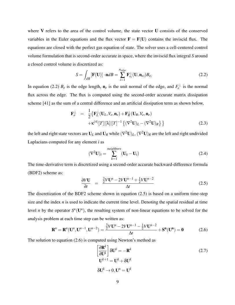
equation (2.5). The unsteady flowfield is computed for 256 timesteps of uniform size dt = 0.4 non-
dimensionalized with the freestream speed of sound and every timestep is converged to machine
precision as shown in Figure 2.3. The flowfield variables at each timestep are then used as input
to the acoustic propagation module, as described in Section 2.4, to determine the noise signature
at the acoustic observer.
12
Figure 2.2: Initialization of the isentropic vortex in the steady state flowfield computed around theNACA-0012 airfoil.
Figure 2.3: Residual convergence for the first three timestep of the unsteady CFD solution
13

2.4 Aeroacoustic Solver: the Two-dimensional FW-H Integra-
tion
After the complex aerodynamic environment around the blade vortex interaction has been deter-
mined, the noise signature of the airfoil at the farfield observer can be computed. Despite the
continuous increase in computational resources, numerical simulations that resolve wave prop-
agation from the nearfield to a farfield observer are still infeasible, hence a viable approach to
predicting farfield noise level is the use of hybrid methods.
In hybrid methods, the finely resolved nearfield flow time history computed by a CFD solver is
used as input to an acoustic integral formulation that predicts the noise radiated to a farfield ob-
server. The acoustic formulations are often based on Lighthill’s acoustic analogy, and in this work
the Ffowcs-Williams and Hawkings (FW-H) acoustic integration has been used, as it is widely
recognized as the workhorse in helicopter aeroacoustic applications [14]. Using the mathemat-
ical theory of distributions, Ffowcs-Williams and Hawkings [46] recombined the Navier-Stokes
equation to arrive at the inhomogeneous wave equation that describes the noise generated by the
relative motion between a body and a surrounding fluid. The FW-H equation can be expressed in
differential form as [46](∂2
∂t− c2
0∂2
∂xi∂x j
)(H( f )ρ′
)=−∂Fiδ( f )
∂xi+
∂Qδ( f )∂t
(2.14)
where
Q = (ρovi +ρ(ui− vi))∂ f∂xi
(2.15)
and
Fj =(
pδi j +ρui(u j− v j
)) ∂ f∂xi
(2.16)
and the Lighthill’s stress tensor, the quadrupole term, has been omitted since it is not used in this
work. Equation (2.15) gives rise to an unsteady monopole-type contribution that can be associ-
ated with mass addition, while the dipole term, equation (2.16), involves an unsteady force. In
equations (2.14), (2.15) and (2.16), the prime denotes perturbation relative to the freestream which
itself is denoted with the subscript o, while xi and t are Cartesian coordinates and time respectively.
The function f (xi) = 0 defines the surface of integration outside of which the solution is sought.
14

Density and pressure are ρ and p, and they are interpreted as the sum of their respective free-stream
values and a perturbation as
ρ = ρo +ρ′
p = po + p′
The fluid velocities are ui, while vi are the surface velocities and co is the freestream speed of
sound. Finally, H( f ) is the Heaviside function while δ( f ) is the Dirac function.
The solution to the inhomogeneous wave equation (2.14) has been the subject of extensive re-
search [13,14,47] and is computed by integrating the quantities in equation (2.15) and (2.16) over
an acoustic integration surface. The integration surface can be the solid surface of the body moving
in the surrounding fluid, as originally proposed by Ffowcs Williams and Hawkings, or an off-body
permeable integration surface as proposed in [14,47]. For three-dimensional problems the acoustic
integration is typically carried out in the time domain [13,14] as described in Chapter 3. However,
for two-dimensional applications Lockard [48] has derived a more efficient integration in the fre-
quency domain that has been used for the two-dimensional BVI case considered in this work.
By assuming uniform rectilinear motion of both the surface and the acoustic observer, the solution
to the two-dimensional differential FW-H equation in the frequency domain reads:
H( f )c20ρ′ = H( f )p′ =−
∮f=0
Fi (ξ,ω)∂G(y,ξ)
∂ξidl−
∮f=0
Q(ξ,ω)G(y,ξ)dl (2.17)
where y is the observer location, ξ = (ξ,η) are the two-dimensional source coordinates on the
integration surface f = 0, ω is the frequency, Q(ξ,ω) and Fi (ξ,ω) are the monopole and dipole
terms in the frequency domain at the source locations and dl is the infinitesimal length along the
surface f = 0.
The function
G(y,ξ) =i
4βe
Mkxβ2 H2
0
(k
β2
√x2 +β2y2
)(2.18)
is the free space Green’s function, where H20 is the Hankel function of second kind of order zero,
and
x = (x−ξ)cosθ+(y−η)sinθ
y =−(x−ξ)sinθ+(y−η)cosθ
15

Figure 2.4: CFD mesh and approximate location of the FW-H integration surface
Here x and y are the observer coordinates, tanθ=V/U with U and V being the freestream Cartesian
velocities of the flow, M =√
U2 +V 2/co is the Mach number and β =√
1−M2 is the Prandtl-
Glauert factor.
Numerical evaluation of the integral in equation (2.17) is performed as follows:
1. Definition of the integration surface f (xi) = 0. The integration surface used in this work is
a collection of edges from the unstructured CFD mesh. This set of edges is selected using a
geometrical distance function criterion. The integration surface is placed four chords away
from the airfoil and its approximate location is shown in Figure 2.4.
2. For every acoustic source on the FW-H acoustic integration surface, assemble the monopole
and dipole term in equations (2.15) and (2.16) for every timestep of the CFD time-integration
process.
3. Apply a window function to the monopole and dipole terms to account for the non-periodicity
of their time histories. In this work the window function proposed by Lockard [48] has been
16

used.
4. Transform the monopole and dipole term to the frequency domain via a Fast Fourier Trans-
form (FFT). While very efficient FFT algorithms are available [49], the one used in this
exercise had to be implemented ex-novo to allow easy access to the source code for tangent
and adjoint differentiation purposes.
Note that steps 3 and 4 require the prior availability of the complete flow time history. For
this reason the acoustic integration in the frequency domain can only be carried out at the
end of the CFD time-integration process and can be considered a post-processing step of the
CFD time-integration.
5. For each frequency in the Fourier Transform and for each observer location, compute the
two-dimensional Green’s function in equation (2.18) to evaluate the integral in equation (2.17)
and determine the total acoustic pressure at the observer in the frequency domain. In this
work the integral is evaluated with a one point Gaussian quadrature.
6. Perform inverse Fourier Transform (iFFT) to recover the acoustic pressure time history at
the observer.
The current acoustic implementation has been validated against two analytical test cases, a monopole
in uniform flow and the scattering of sound by an edge [48, 50].
The complex potential for the monopole in uniform flow is given by Lockard [48] as
φ(x, t) = AeiωtG(y,ξ) (2.19)
where A is the amplitude, ω is the frequency, t is time and G(y,ξ) is the Green’s function defined
in equation (2.18). Equation (2.19) gives the value of the potential at any point in space and
time and the variables needed for the FW-H integration are obtained by taking the real part of
p′ = −ρo(∂φ
∂t+Ui
∂φ
∂xi), u′i =
∂φ
∂xiand using the isentropic condition ρ′ = p′/c2
o. The FW-H is
then validated by first evaluating the exact acoustic pressure at the observer location. Then all
the variables needed to evaluate the FW-H integral in equation (2.17) are evaluated at the FW-H
surface and the integration is performed. The acoustic prediction is then compared to the exact
analytical solution. Results for this test case are presented in Figure 2.5: Figure 2.5(a) shows
17

(a) Comparison between the exact acoustic pressureand the one computed by the two-dimensional FW-H acoustic integration for an observer at r = 500m,θ = 180deg for a monopole in uniform flow
(b) Directivity plot for the monopole in uniform flowfor an observer at r = 500m
Figure 2.5: Validation of the two-dimensional acoustic integration for the monopole in uniformflow test case [48]
excellent agreement between the exact and the predicted acoustic pressure time histories for an
observer at a radial distance r = 500m and an azimuthal location θ = 180deg. Figure 2.5(b) shows
the root mean square of the acoustic pressure for the exact solution and the acoustic integration at
different azimuthal locations but for the same radial distance r = 500m, confirming the accuracy
of the acoustic integration.
The same procedure is followed for the scattering of sound by an edge. A vortex of strength k
moves around the edge of a semi-infinite plate along the path shown in Figure 2.6. The vortex
reaches its maximum speed when it is closest to the plate, reaching a Mach number M = 0.001.
The potential for this flow is given by Crighton [50] as:
φ(x, t) =2√
2
[M2(r− t)2 +4]14
sin(θ
2)
r12
(2.20)
where r =√
x2 + y2 is the radial distance from the origin to a general (x,y) location in the 2D
plane, non dimensionalized with the distance b in Figure 2.6 and θ is the angle measured relative
to the positive x-axis. Results for this case are shown in Figure 2.7. Figure 2.7(a) compares
the acoustic-pressure time histories for the exact solution and the acoustic integration at a radial
18

Figure 2.6: Schematic of the scattering by an edge from Rumpfkeil [51]
distance r = 50m and θ = 0deg, while Figure 2.7(b) shows the exact and predicted root mean
square of the acoustic pressure for an observer at r = 50m and different azimuthal locations. In
both cases the agreement between the exact solution and the acoustic integration is excellent.
2.5 Tangent and Adjoint Formulations for the Two-dimensional
Aeroacoustic Problem
To perform the efficient gradient-based aeroacoustic optimization of the NACA-0012 airfoil in
blade-vortex interaction the adjoint sensitivities need to be derived for the coupled aeroacoustic
problem. First, the tangent and adjoint sensitivities for the airfoil in vortex interaction are pre-
sented: for simplicity the sensitivities are derived for a BDF1 time discretization and the derivation
closely follows that of Mani and Mavriplis [35]. The sensitivity formulation is then extended to
include the tangent and adjoint acoustic sensitivities, to realize the coupled aeroacoustic sensitivity.
The tangent sensitivity is derived first, while the adjoint sensitivity is obtained by transposing and
reversing all the operations performed in forward mode. The tangent sensitivity is then validated
with respect to the complex step method [52,53], while the adjoint sensitivity is validated with the
19

(a) Exact and FWH acoutic pressure solution for anobserver at r = 50m and θ = 0deg for a vortex passingover an edge
(b) Directivity plot for the vortex over edge flow for anobserver at r = 50m
Figure 2.7: Validation of the acoustic solver for the scattering of sound by an edge [50]
duality relation [54] with the tangent model.
2.5.1 Sensitivity Analysis Formulation for Airfoil in Vortex Interaction
To derive the tangent and adjoint sensitivities for the airfoil in vortex interaction, the objective
function Ln at the end of the time-integration process can be expressed as
Ln = Ln (Un(D),x(D)) (2.21)
where D is the vector of design variables and x(D) is the vector of mesh coordinates that depends
on the design variables, but not on time.
Differentiating equation (2.21) with respect to one design variable yields:
dLn
dD=
∂Ln
∂UndUn
dD+
∂Ln
∂xdxdD
(2.22)
The flow residual at each timestep for a BDF1 time discretization scheme is given as
Rn = Rn (Un(D),Un−1(D),x(D))=
V(Un−Un−1)
∆t+Sn(Un,n) = 0 (2.23)
20

and an expression for dUn
dD to be used in equation (2.22) is obtained by differentiating equation
(2.23) with respect to a design variable D
∂Rn
∂UndUn
dD+
∂Rn
∂Un−1dUn−1
dD+
∂Rn
dxdx∂D
= 0 (2.24)
and solving for the flow tangent sensitivity at timestep n as
dUn
dD=−
[∂Rn
∂Un
]−1(∂Rn
∂Un−1dUn−1
dD+
∂Rn
dxdx∂D
)(2.25)
In equation (2.25),[
∂Rn
∂Un
]is the exact second-order-accurate Jacobian of equation (2.23) that is
inverted using the GMRES - Krylov algorithm used in the analysis problem. Equation (2.25)
represents a forward integration in time where the initial condition dU0
dD is given by the linearization
of the vortex equations with respect to the design variables.
The term dxdD is obtained from
[K]dxdD
=dxsur f
dD(2.26)
where [K] is the stiffness matrix of the mesh deformation problem as described in Section 2.2 anddxsur f
dD is the forward sensitivity of the mesh boundary nodes with respect to the design variables
computed by linearization of the geometry paramterization described in Section 2.2. The system
in equation (2.26) is solved with the same GMRES-Krylov algorithm described in Section 2.2.
Once the term dUn
dD has been computed as per equation (2.25), the objective function sensitivity at
the final timestep can be evaluated with the matrix vector products described in equation (2.22).
Equation (2.22) gives the sensitivity of the objective function in equation (2.21) with respect to one
design variable D. However, for gradient-based optimization, the sensitivity of the objective func-
tion with respect to the full vector of design variables D is needed. Hence, the expensive forward
time integration in equation (2.25) would need to be repeated for every design variable in the vec-
tor D. A more efficient approach is to compute the adjoint sensitivity of the objective function by
transposing and reversing all the operations performed in the tangent mode. Transposing equation
(2.22) gives the reverse linearization of the objective function in equation (2.21)
dLn
dD
T=
dUn
dD
T∂Ln
∂Un
T
+dxdD
T∂Ln
∂x
T
(2.27)
The term dUn
dDT
is obtained by transposing equation (2.25) as
dUn
dD
T=−
(∂Rn
∂Un−1dUn−1
dD+
∂Rn
∂xdxdD
)T [∂Rn
∂Un
]−T
(2.28)
21
So that equation (2.27) becomes
dLn
dD
T=−
(dUn−1
dD
T∂Rn
∂Un−1
T
+dxdD
T∂Rn
∂x
T)[
∂Rn
∂Un
]−T∂Ln
∂Un
T
+dxdD
T∂Ln
∂x
T
(2.29)
The flow adjoint variable at time level n is now defined as
Λnu =
[∂Rn
∂Un
]−T∂Ln
∂Un
T
(2.30)
And equation (2.29) becomes
dLn
dD
T=−dUn−1
dD
T∂Rn
∂Un−1
T
Λnu +
dxdD
T(
∂Ln
∂x
T
− ∂Rn
∂x
T
Λnu
)(2.31)
The first term in equation (2.31) depends on the sensitivity dUn−1
dDT
at the previous timestep, which
can be computed by evaluating equation (2.28) at timestep n−1 as
dUn−1
dD
T
=−(
∂Rn−1
∂Un−2dUn−2
dD+
∂Rn−1
∂xdxdD
)T [∂Rn−1
∂Un−1
]−T
(2.32)
Substituting equation (2.32) into equation (2.31) and defining a new adjoint variable at timestep
n−1 as
Λn−1u =
[∂Rn−1
∂Un−1
]−T∂Rn
∂Un−1
T
Λnu (2.33)
equation (2.31) becomes
dLn
dD
T=−dUn−2
dD
T∂Rn−1
∂Un−2
T
Λn−1u +
dxdD
T(
∂Ln
∂x
T
−n
∑i=n−1
∂Ri
∂x
T
Λiu
)(2.34)
Equation (2.34) now depends on the sensitivity dUn−2
dDT
at timestep n− 2, hence equation (2.31)
represents a backward time integration for the flow adjoint variable that at a given time level k is
given by
Λku =−
[∂Rk
∂Uk
]−T [∂Rk+1
∂Uk
T
Λk+1u
](2.35)
where[
∂Rn
∂Un
]Tis the transpose of the second-order-accurate flow Jacobian that is inverted iteratively
using a GMRES - Krylov algorithm preconditioned with a colored Gauss - Seidel iteration scheme.
The final (initial) term dU0
dDT
is taken from the linearization of the vortex equations with respect to
22

the design parameter in reverse mode. At the end of the backward time integration the sensitivity
vector is
dLn
dD
T=
dxdD
T(
∂Ln
∂x
T
−n
∑i=1
∂Ri
∂x
T
Λiu
)(2.36)
By transposing equation (2.26), the term dxdD
Tbecomes
dxdD
T=
dxsur f
dD
T[K]T (2.37)
and substituting equation (2.37) into equation (2.36) the mesh adjoint problem can be defined as
Λx = [K]−T
[∂Ln
∂x
T
−n
∑i=1
∂Ri
∂x
T
Λiu
](2.38)
The system is solved with a Jacobi preconditioned GMRES - Krylov algorithm. Finally, the sensi-
tivity vector dLn
dDT
is given by the product
dLn
dD
T=
dxsurfdD
TΛx (2.39)
where the term dxsurfdD
Tis the known sensitivity of the boundary nodes with respect to the design
variables. For the two-dimensional optimizations presented in Chapter 4 the linear systems in
equations (2.35) and (2.38) are both converged to machine precision as shown in Figure 2.8
In the case of a time-integrated objective function, equation (2.21) is modified as
Lg = Lg (L1,L2 · · · ,Ln) (2.40)
and its forward linearization is
dLg
dD= ∑
n
[∂Lg
∂Ln∂Ln
∂UndUn
dD+
∂Lg
∂Ln∂Ln
∂xdxdD
](2.41)
with dUn
dD and dxdD that are still computed from equations (2.25) and (2.26). The term ∂Lg
∂Ln is the
derivative of the global (time-integrated) objective function Lg with respect to the local (instanta-
neous) objective function Ln. Transposing equation (2.41) gives the adjoint or reverse linearization
of equation (2.40) as
dLg
dD
T= ∑
n
[dUn
dD
T∂Ln
∂Un
T∂Lg
∂Ln
T
+dxdD
T∂Ln
∂x
T∂Lg
∂Ln
T]
(2.42)
23

Figure 2.8: Residual convergence for the flow adjoint problem at a generic timestep and the finalmesh adjoint problem
Substituting again equation (2.28) into equation (2.42) and following the same rationale used to
arrive at equation (2.35), the flow adjoint equation for a time-integrated objective function now
becomes
Λku =−
[∂Rk
∂Uk
]−T [∂Lk
∂Uk
T∂Lg
∂Lk
T
+∂Rk+1
∂Uk
T
Λk+1u
](2.43)
and at the end of the backward time integration process the mesh adjoint equation can be computed
as
Λx = [K]−Tn
∑i=1
[∂Lg
∂Li
T∂Li
∂x
T
− ∂Ri
∂x
T
Λiu
](2.44)
so that the final sensitivity in equation (2.42) becomes
dLg
dD
T=
dxsurfdD
TΛx (2.45)
Hence, as described by Mani and Mavriplis [35], the only difference between the time-integrated
and the non-time-integrated objective function is the pre/post multiplication of the terms ∂Ln
∂Un and∂Ln
∂x by the global-to-local sensitivity ∂Lg
∂Ln for the forward/adjoint sensitivity respectively. The two
24

terms ∂Ln
∂UnT
and ∂Ln
∂xT
drive the backward adjoint time integration: in the case of the acoustic opti-
mization these terms come from the adjoint linearization of the FW-H acoustic module as explained
in Section 2.5.2.
Verification of the Aerodynamic Sensitivities for the Airfoil in Blade-vortex Interaction
The tangent linearization has been verified against the complex step method [52,53]. Any function
f (x) operating on a real variable x can be used to compute both the function and its derivative
f ′(x) if the input variable x and all the intermediate variables used in the discrete evaluation of
f (x) are redefined as complex variables. In this case for a complex input the function will produce
a complex output. A Taylor series of the now complex function f (x+ ih) , where h is a small
step-size and i is the imaginary unit, reads
f (x+ ih) = f (x)+ ih f ′(x)+O(h2) (2.46)
from which the real part is simply the function value at x, while from the imaginary part the
function derivative can be easily evaluated as
f ′(x) =Im [ f (x+ ih)]
h(2.47)
Despite requiring a step size, as in the case of finite-differencing, the complex step method is
insensitive to small step-sizes since no differencing is required. Hence, by using a step size h =
10−31 the tangent formulation for the blade vortex interaction case can be verified to machine
precision against the complex step method.
The adjoint sensitivities are then verified with the duality relationship [54] between the tangent and
the adjoint formulations. Table 2.1 shows the comparison between the adjoint linearization and
the complex step method for the 7th design variable for the time-integrated aerodynamic objective
function defined in equation (4.1). The error between the complex step method and the flow adjoint
is of the order of machine precision, thus verifying the correctness of the adjoint linearization.
25

Table 2.1: Complex step validation of the 7th design sensitivity of the flow adjoint.Adjoint Complex Error
-1.7854017702037789E-01 -1.7854017702038E-01 -2.10942374678780E-15
2.5.2 Sensitivity Analysis for the FW-H Equation
To enable adjoint-based aeroacoustic optimization the tangent and adjoint differentiation of the
FW-H acoustic integration needs to be derived. The linearizations of the acoustic integrals will
then be coupled to the corresponding tangent and adjoint linearizations of the CFD flow solver to
realize the tangent and adjoint linearizations of the coupled aeroacoustic problem.
The functional dependencies for the quantities in the acoustic integrals in equation (2.17) are shown
in equation (2.48)
Q = Q(xs(D),U(D),ω)
Fi = Fi (xs(D),U(D),ω) (2.48)
G = G(xs(D),xo,ω)
∂G∂xs
=∂G∂xs
(xs(D),xo,ω)
where xs(D) is the discrete source location on the discrete FW-H integration surface, xo is the
observer location and ω is the frequency. From equation (2.48) it is evident that the monopole and
dipole terms depend on the design parameters D through both the FW-H surface geometry and the
input CFD solution. The acoustic pressure at the observer can then be expressed as
p′(D,ω) = FWH(U(D,ω),x(D),ω) (2.49)
where FWH(U(D,ω),x(D),ω) represents all the discrete operations necessary to evaluate equa-
tion (2.17) numerically, as described in Section 2.4. Differentiation of equation (2.49) with respect
to one design variable yields the pressure sensitivity at the observer as
d p(D,ω)
dD= ∑
n
∂FWH∂Un
FWH
dUnFWH
dD+
∂FWH∂xFWH
dxFWH
dD(2.50)
where dUnFWH
dD is the tangent CFD solution at the n− th timestep evaluated at the FW-H surface
location, and dxFWHdD is the CFD mesh sensitivity at the FWH integration surface. The matrices
26

∂FWH∂UFWH
and ∂FWH∂xFWH
have been obtained by forward linearization of each component in the acoustic
integration.
The time-integrated acoustic objective function used in this work is the overall sound pressure level
(OSPL) at the observer location, defined as in equation (2.51):
LFWH = OSPL(p(D)) = 20log10
(p′RMS
p0
)(2.51)
Here p′RMS is the root mean square of the acoustic pressure at the observer as computed by the
FW-H acoustic integration and p0 = 20µPa is a reference pressure. Thus the final form of the
aeroacoustic objective sensitivity reads:
dLFWH
dD=
∂SPL∂p
d pdD
=∂SPL
∂p
[∑n
∂FWH∂Un
FWH
dUnFWH
dD+
∂FWH∂xFWH
dxFWH
dD
](2.52)
= ∑n
∂LnFWH
∂UnFWH
dUnFWH
dD+
∂LFWH
∂xFWH
dxFWH
dD
The flow and the acoustic analysis codes are loosely coupled and, as stated before, the FW-H
acoustic propagation model can be considered a post-processing step of the unsteady CFD simu-
lation. All the two-dimensional aeroacoustic simulations are carried out on a computational mesh
consisting of approximately 60000 elements. The non-conserved variables of the CFD solution
must be extracted at the source locations on the FW-H integration surface for the complete time
history to assemble the monopole and dipole terms in equations (2.15) and (2.16). Since the CFD
solver is a cell-centered solver and the FW-H surface is a concatenation of edges from the un-
structured CFD mesh, an unlimited least-square gradient reconstruction procedure is employed to
guarantee second-order accuracy while extracting the CFD data at the acoustic surface location.
The edges of the FW-H surface are chosen using a wall distance criterion four chords away from
the airfoil and the approximate location of the integration surface is shown in Figure 2.4. The ex-
tracted CFD solution time history is then used as input to the FW-H acoustic solver and the acoustic
objective function can be computed. The same procedure is followed to couple the tangent flow
and the tangent acoustic codes. The complete time history of the tangent flow sensitivity must be
reconstructed at the FW-H integration surface, then both the flow and the mesh sensitivities at the
integration surface can be passed as input to the tangent FW-H solver and finally the sensitivity
of the time-integrated objective function, the overall sound pressure level at the observer, can be
27

(a) Propagated and computed acoustic pressure sensi-tivity for an observer 0.4 chords away from the FW-Hintegration surface
(b) Propagated and computed acoustic pressure sensi-tivity for an observer 1.5 chords away from the FW-Hintegration surface
Figure 2.9: Comparison of FW-H propagated and CFD computed acoustic pressure sensitivity atdifferent observer locations highlighting the detrimental effect that numerical dissipation has onthe computed acoustic pressure sensitivity as the observer is moved to the far field.
computed. Hence, the sensitivity in equation (2.52) can be computed once the vectors dUn
dD and dxdD
are known at the FW-H surface from the flow and mesh tangent problem. Therefore the tangent
FW-H solver can be considered a post-processing step of the flow tangent problem. A compari-
son between the propagated and the computed observer acoustic pressure sensitivity is shown in
Figure 2.9 for two different observer locations. In Figure 2.9(a) the observer is placed underneath
the airfoil at the center of a CFD cell approximately 0.4 chords away from the FW-H integration
surface while in Figure 2.9(b) the observer is placed approximately 1.5 chords away and for both
cases the acoustic pressure sensitivity computed by the tangent flow solver can be compared to
that propagated by the tangent FW-H solver. Figure 2.9 shows good agreement between the two
codes. Note that the tangent CFD solution consistently underestimates all the peaks in the sensitiv-
ity time history, a consequence of the numerical dissipation associated with the employed spatial
discretization. Furthermore, this behaviour deteriorates as the observer is placed further away from
the FW-H integration surface.
Transposing equation (2.52) yields the adjoint linearization of the acoustics objective fuction as
28

Table 2.2: Finite difference validation of the 7th design sensitivity.Adjoint FD Error
-3.1819940460451508E-03 -3.17975314778490E-03 2.24089826024758E-06
dLFWH
dD
T= ∑
n
dUn
dD
T∂Ln
FWH∂Un
T
+dxdD
T∂LFWH
∂x
T
(2.53)
The terms ∂LnFWH
∂UnFWH
Tand ∂LFWH
∂xT
are known once the products ∂FWH∂UFWH
T ∂SPL∂p′
Tand ∂FWH
∂xFWH
T ∂SPL∂p′
Thave
been evaluated. These two matrix - vector products are the adjoint linearization of the discrete
FW-H equation and are obtained by transposition of the corresponding matrices in the forward
linearization. Equation (2.53) is now in the form of equation (2.42) and the backward time inte-
gration described in Section 2.5.1 can start with the terms ∂Ln
∂UnT=
∂LnFWH
∂UnFWH
T= ∂FWH
∂UFWH
T ∂SPL∂p
Tand
∂L∂x
T= ∂LFWH
∂xT= ∂FWH
∂xFWH
T ∂SPL∂p
Tprovided by the adjoint linearization of the acoustic integration.
Hence, the adjoint of the acoustic module can be considered a preprocessing step to the flow ad-
joint solver described in Section 2.5.1: once the two terms ∂LnFWH
∂UnFWH
Tand ∂LFWH
∂xT
are known the flow
adjoint solver can start as described in Section 2.5.1.
The tangent and FW-H integration have been verified with a finite-difference approach as the
complex-step method [52, 53] is not applicable in this case since the acoustic analysis equation
itself includes complex variables via the Fourier transform and the Green’s function in equation
(2.17). The adjoint solver has then been validated by the duality-relation [54] to the tangent solver
to machine precision. Table 2.2 shows the finite difference validation of the 7th adjoint design
sensitivity. A second-order-accurate centered finite-difference scheme with a step δD = 10−4 has
been used.
With minor modifications the coupling strategy for the two-dimensional tangent and adjoint aeroa-
coustic linearizations will be applied to the three dimensional problem, the main differences re-
sulting from the time-domain formulation for the three-dimensional FW-H acoustic integration as
described in Chapter 3.
29

Chapter 3
Three Dimensional Aeroacoustic Problem
for Helicopter Rotors
The three-dimensional adjoint-based multidisciplinary design capability is introduced in this chap-
ter. The design tool encompasses the three disciplines of aerodynamics, structural mechanics and
aeroacoustics. First, the solver for each discipline is presented, with particular emphasis on the
acoustic integration. The coupling of the three discipline is then discussed and the linearization of
the coupled multidisciplinary unsteady problem is introduced.
3.1 Aerodynamic Solver
The base flow solver used in this work is the NSU3D unstructured mesh Reynolds-averaged
Navier-Stokes solver [41,55]. NSU3D has been widely validated for steady-state and time-dependent
flows and is augmented with a discrete tangent and adjoint sensitivity capability which has been
demonstrated previously for optimization of steady-state and time-dependent flow problems. As
such, only a concise description of these formulations will be given in this thesis, with additional
details available in references [32,54,56]. The flow solver is based on the conservative form of the
Navier-Stokes equations which may be written as:
∂u(x, t)∂t
+∇ ·F(u) = 0 (3.1)
30

For moving mesh problems these are written in arbitrary Lagrangian-Eulerian (ALE) form as:
∂V u∂t
+∫
dB(t)[F(u)− xu] ·ndB = 0 (3.2)
Here V is the control volume, x is the vector of mesh face velocities, n is the unit normal of
the face, and B(t) is the surface area of the time varying control volume. The state vector u
consists of the conserved variables and the Cartesian flux vector F = (Fx,Fy,Fz) contains both
inviscid and viscous fluxes. The equations are closed with the perfect gas equation of state and the
Spalart-Allmaras turbulent eddy viscosity model [57] for all cases presented in this work. The time
derivative term is discretized using a second-order accurate backward-difference formula (BDF2)
scheme and the implicit residual is solved using Newton’s method. The Jacobian matrix is in-
verted iteratively using a line-implicit agglomeration multigrid scheme that can also be used as a
preconditioner for a GMRES Krylov solver [58]. For the remainder of this chapter, the system of
non-linear equations for the CFD analysis problem will be represented by the generalized notation:
R(u,x) = 0 (3.3)
where the vector u denotes the flow values, x represents the CFD mesh coordinates, and equation
(3.3) denotes the simultaneous solution of all time steps.
3.2 Structural Dynamics Solver
The structural dynamics of the blade are modeled with an Hodges-Dowell [59], non-linear, bend-
twist finite-element model that is well suited for rotary-wing aircraft structures. The model has
previously been developed and coupled to the NSU3D flow solver for both steady [60, 61] and
time-dependent problems [62]. Figure 3.1 shows a typical beam with 15 degrees of freedom per
element to accommodate bend wise, lag wise, axial and torsional displacements. The second-order
equation of motion for the beam can be expressed as: Mq+Cq+Kq = F . Here [M], [C] and [K]
are mass, damping and stiffness matrices of the system of equations representing the beam. The
vector F=F(t) is the forcing vector, while q represents the displacements along all degrees of free-
dom. This set of equations can be reduced to a first-order system and solved using a second-order
backward difference formula (BDF2) time integration with standard Newton-type linearization and
31

Figure 3.1: Beam element with flap, lag, torsional and axial (total 15) degrees of freedom.
sub-iterations to efficiently invert the implicit system: [I]Q+ [A]Q = F, where [I] is the identity
matrix, Q = [q, q]T , F = [0, [M]−1F]T and [A] =[
0 −[I][M]−1[K] [M]−1[C]
]. The residual of the structural
equations can be defined as: J = [I] Q+[A] Q−F = 0, and can be expressed in a simplified form
as:
J(Q,F) = 0 (3.4)
The beam model for the applications presented in Chapter 4 consists of 20 elements per blade
and has been validated for the standard HART-II rotor case [5] by comparing its natural frequency
predictions with the predictions from other reliable computational structural dynamics models,
such as UMARC [63] and DLR [64], as shown in Table 3.1. Tangent and adjoint linearizations
of the structural model have been developed and coupled to the NSU3D flow solver as shown in
previous work [62].
32

Table 3.1: Comparison of HART-II Natural Frequencies [65]Modes Present Model UMARC DLRFlap 1 1.104 1.112 1.125Flap 2 2.802 2.843 2.835Flap 3 5.010 5.189 5.168
Torsion 1 3.878 3.844 3.845
3.2.1 Fluid-structure Interface
In addition to the solution of the aerodynamic problem and the structural dynamics problem, the
solution of the fully coupled time-dependent aeroelastic problem requires the exchange of aerody-
namic loads from the CFD solver to the beam structure, which in turn returns surface displacements
to the fluid flow solver. In practice, the fluid-structure-interface computes forces at each CFD sur-
face mesh point F(x,u) by integrating the surface stresses (pressure and shear) over the surface
area associated with each surface grid point. These forces are then projected onto the beam finite-
element basis functions where they are assembled in the form of forces on the beam finite-element
nodal locations denoted as Fb. Conversely, once the beam deflections have been computed, the
structural displacements are transferred back to the surface CFD mesh in a similar manner. The
governing equations for the FSI can be written in residual form as:
S(Fb,x,u) = Fb− [T (Q)]F(x,u) = 0
S′(xs,Q) = xs− [T (Q)]T Q = 0 (3.5)
In equation (3.5), [T ] represents the rectangular transfer matrix that projects the CFD loads F(x,u)
on the beam model, while its transpose [T ]T is used to obtain the CFD surface coordinates xs from
the CSD degrees of freedom Q
3.3 Prescribed Blade Motion
The time-dependent simulation of a rotor in forward flight requires a prescribed blade motion
capability, in particular the individual blade cycling pitching motion must be superimposed with a
simple solid body rotation of the entire rotor blade system and CFD mesh that contains the rotor.
33

For each blade, the time-dependent pitch angle can be represented by a combination of mean pitch
angle and several harmonic components:
θ = θ0 +n
∑i=1
θci cos(iψ)+n
∑i=1
θsi sin(iψ) (3.6)
where ψ is the rotor azimuth. Only one harmonic is used to attain the required thrust and moments
values, hence i = 1, and the control parameters Dpitch = [θ0,θ1c,θ1s] are to be chosen such that
the rotor is trimmed, where θ0 is the collective and θ1c,θ1s are the two cyclic pitch parameters.
To incorporate rotor pitch actuation in the CFD simulation two additional equations need to be
considered:
• a pitch actuation equation
Sθ(xsθ,xs,Dpitch) = 0 (3.7)
• an azimuthal mesh rotation equation
Sψ(x,xθ) = 0 (3.8)
Evaluation of equation (3.7) pitches the blade and yields a new set of surface grid coordinates xsθ.
Then, to avoid negative-volume cells in the region surrounding the blade, the interior mesh must be
deformed. This is accomplished with the mesh deformation algorithm described in Section 3.5 and
results in a new set of interior mesh coordinates denoted xθ. Equation (3.8) is then applied to rotate
the entire mesh to the current azimuthal location and results in the final set of grid coordinates x.
3.4 Geometry Parameterization Facility
To perform blade shape optimization, a shape parameterization technique must be implemented.
The blade parameterization technique defines the blade surface, and in turn the intial CFD surface
mesh coordinates xso, as a function of a set of shape design variables, D. Hence the blade surface
mesh points are computed as the solution of a parameterization equation that, in residual form,
reads
BCAD (xso,D) = 0 (3.9)
The specific geometry parameterization used in this work is discussed in Chapter 4.
34
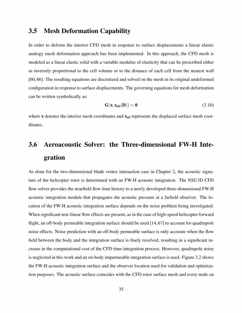
3.5 Mesh Deformation Capability
In order to deform the interior CFD mesh in response to surface displacements a linear elastic
analogy mesh deformation approach has been implemented. In this approach, the CFD mesh is
modeled as a linear elastic solid with a variable modulus of elasticity that can be prescribed either
as inversely proportional to the cell volume or to the distance of each cell from the nearest wall
[60,66]. The resulting equations are discretized and solved on the mesh in its original undeformed
configuration in response to surface displacements. The governing equations for mesh deformation
can be written symbolically as:
G(x,xsθ(D)) = 0 (3.10)
where x denotes the interior mesh coordinates and xsθ represents the displaced surface mesh coor-
dinates.
3.6 Aeroacoustic Solver: the Three-dimensional FW-H Inte-
gration
As done for the two-dimensional blade vortex interaction case in Chapter 2, the acoustic signa-
ture of the helicopter rotor is determined with an FW-H acoustic integration. The NSU3D CFD
flow solver provides the nearfield flow time history to a newly developed three-dimensional FW-H
acoustic integration module that propagates the acoustic pressure at a farfield observer. The lo-
cation of the FW-H acoustic integration surface depends on the noise problem being investigated.
When significant non-linear flow effects are present, as in the case of high-speed helicopter forward
flight, an off-body permeable integration surface should be used [14,67] to account for quadrupole
noise effects. Noise prediction with an off-body permeable surface is only accurate when the flow
field between the body and the integration surface is finely resolved, resulting in a significant in-
crease in the computational cost of the CFD time-integration process. However, quadrupole noise
is neglected in this work and an on-body impermeable integration surface is used. Figure 3.2 shows
the FW-H acoustic integration surface and the observer location used for validation and optimiza-
tion purposes. The acoustic surface coincides with the CFD rotor surface mesh and every node on
35

Figure 3.2: Acoustic integration surface and observer location: the observer is stationary in theplane of the rotor two radii from the rotor hub at ψ = 180 deg.
the surface is an acoustic source that produces an acoustic pressure at the observer location via the
FW-H integration process.
Acoustic Analysis Formulation: the FW-H Integration in the Time Domain
As mentioned in Chapter 2, the acoustic integration in three dimension is typically carried out in
the time domain following the derivation from Farassat [13] using the variables
Ui =
(1− ρ
ρo
)vi +
ρui
ρo
Li = p′n j +ρui (un− vn) (3.11)
as proposed by Di Francescantonio [47]. In equation (3.11), p′ = p− po is the acoustic pressure, ni
is the unit normal of the acoustic surface, un = uini and vn = vini are the flow and surface velocities
36

in the direction normal to the integration surface, and for the on-body solid acoustic integration
surface used in this work u = v. The integral solution is then given, neglecting the quadrupole
term, by equation (3.12)
4πp′T (y, t) =∫
f=0
[ρo(Un +Un
)r(1−Mr)2
]ret
dS
+∫
f=0
[ρoUnK
r2(1−Mr)3
]ret
dS
4πp′L =1co
∫f=0
[Lr
r(1−Mr)2
]ret
dS (3.12)
+∫
f=0
[Lr−LM
r2(1−Mr)2
]ret
dS
+1co
∫f=0
[LrK
r2(1−Mr)3
]ret
dS
4πp′(y, t) = 4πp′T (y, t)+4πp′L(y, t)
where y is the observer location, t is the observer time, r is the distance between the source x and
the observer y with normalized cartesian components ri, M is the acoustic source Mach number
and
Un =Uini
Mr = Miri
Lr = Liri (3.13)
LM = LiMi
K = rMr + co(Mr−M2)
Equation (3.12) requires the evaluation of the integrals at the emission or retarded time τ: for a
given observer location y and time t the retarded time must be computed via the solution of the
nonlinear equation (3.14)
τ = t− r(x(τ),y(t))/co (3.14)
where r(x(τ),y(t)) is the distance between the source x at the emission time τ and the observer y at
the observer time t. This approach has been followed in most acoustic-analogy-based codes [14].
37

However, by regarding the source time as the primary time one can choose the source time for an
acoustic source and determine when the signal will reach the observer using equation (3.15)
t = τ+ r(x(τ),y(t))/co (3.15)
where τ is again the source time and t is the reception time, i.e. the time at which the acoustic
disturbance reaches the observer. Equation (3.15), a rearrangement of equation (3.14), is easier to
solve than its retarded time counterpart as the observer motion is usually simpler than the motion
of the acoustic integration surface. For each acoustic source a sequence of uniformly spaced source
times leads to a sequence of unequally spaced observer times as each source has a different source-
to-observer distance, hence the acoustic pressure time history for each source must be interpolated
at the desired observer time to determine the final acoustic pressure at the observer location. A
comparison of the retarded time and the source-time-dominant algorithm is given in [68].
The source-time-dominant algorithm has been followed in this work since it allows a seamless
integration of the acoustic module with the CFD solver. The aerodynamic and aeroacoustic time
integration proceed simultaneously and the acoustic surface of integration is the unstructured sur-
face mesh of the rotor. Hence each node of the CFD surface grid corresponds to an acoustic source.
The FW-H acoustic integration in the time domain can be summarized as follows:
1. At every CFD timestep and for every acoustic source compute the flow and surface time
derivatives Un, Un, Lr and Mr in equations (3.12) and (3.13) as
Un =dUi
dtni
Un =Uidni
dt
Lr =dLi
dtri
Mr =dMi
dtri
The time derivatives are based on a BDF2 time discretization with the exception of the source
acceleration term Mr that is approximated with a second-order-accurate central difference
scheme.
2. At every timestep and for every acoustic source assemble the terms in equations (3.11) and
(3.13).
38

3. At every timestep and for every acoustic source evaluate the acoustic integrals in equation
(3.12) using a one point Gaussian quadrature to determine the acoustic pressure time history
at the observer. In general, the relative distance between the observer and the acoustic source
is different for each source, hence a sequence of uniformly spaced source times will result
in a sequence of unequally spaced observer reception times for every acoustic source.
4. At the end of the CFD time-integration process build the total acoustic pressure at the ob-
server by linear interpolation of each source acoustic pressure at a sequence of specified
observer times.
5. Compute the aeroacoustic objective to be used in the optimizations presented in Chapter 4.
LFWH = p′RMS =
√∑
Nsamplei=1 p′2(D)
Nsample(3.16)
where Nsample is the number of samples in the observer acoustic pressure time history and D
is the vector of design variables.
The current implementation of the FW-H integral equation has been validated against the PSU-
WOPWOP [68] acoustic code for the HART-II flexible rotor in trimmed forward flight as shown
in Figure 3.3. The rotor has a freestream Mach number of M = 0.095 with a tip Mach number
of Mtip = 0.638, a shaft angle αsha f t = 5.4deg and a Reynolds Number of 2 million. The corre-
sponding rotor rotational speed is Ω = 1041 RPM (advance ratio µ = 0.15). The CFD simulation
has been carried out for two rotor revolutions on a mesh consisting of approximately 2.32 million
nodes with a 2-degree timestep, 6 CFD/CSD coupling iterations per time step and a stationary in-
plane observer located two radii from the rotor hub at an azimuthal angle ψ = 180 deg as shown in
Figure 3.2 and described in Table 3.2. Two different observer time windows are shown in Figure
3.3: an extended time window, Figure 3.3(a), and the observer time window targeted during the op-
timization, Figure 3.3(b). In both cases agreement between the new FW-H implementation and the
legacy PSU-WOPWOP code [68] is excellent. The effect that blade flexibility has on the predicted
total acoustic pressure is investigated in Figure 3.4: the positive pressure peak is more pronounced
in the flexible case while the negative pressure peak is significantly reduced as a consequence of
blade deformation. A comparison of the rigid and flexible blades is shown in Figure 3.5 together
39

Table 3.2: Observer location for the acoustic objective function with respect to the rotor hub, Rbeing the rotor radius
x y z2R 0 0
with a surface countour plot of the pressure coefficient. All four blades show different deforma-
tion characteristics due to the corresponding different aerodynamic environment they experience
during trimmed forward flight: the largest flap displacement is attained at ψ = 180 deg while the
smallest happens at ψ = 0 deg.
3.7 Fully Coupled Multidisciplinary Analysis Problem
After introducing each discipline separately, the solvers for aerodynamics, structural mechanics
and aeroacoustics will now be linked together to realize the multidisciplinary analysis problem for
rotorcraft design.
For a given design geometry, the analysis problem consists of a coupled system of equations that
needs to be solved at every timestep. At the beginning of the CFD time-integration process, equa-
tion (3.17) defines the new blade shape. At every timestep blade pitch control is applied by explicit
evaluation of equation (3.18): the cyclic pitching acts directly on the deflected blade shape co-
ordinates xs, although these depend on the original undeflected blade surface coordinates xso and
reduce to these values at the beginning of the solution procedure prior to the solution of the struc-
tural equations. Next, the combined surface displacements from equations (3.17) and (3.18) are
propagated to the interior CFD mesh by iterative solution of the mesh deformation problem in
equation (3.19), and the deformed mesh is then rigidly rotated through explicit evaluation of equa-
tion (3.20). The fully coupled fluid-structure problem can now be solved by performing multiple
coupling iterations on each discipline using the latest available values from the other disciplines.
The flow residual equations, equation (3.21), are solved iteratively using the updated grid coordi-
nates x, and the resulting flow variables u are used to compute the aerodynamic forces that are then
40
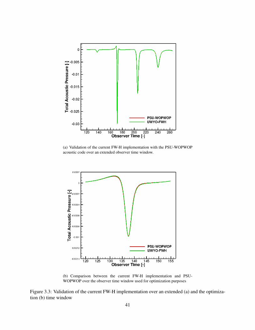
(a) Validation of the current FW-H implementation with the PSU-WOPWOPacoustic code over an extended observer time window.
(b) Comparison between the current FW-H implementation and PSU-WOPWOP over the observer time window used for optimization purposes
Figure 3.3: Validation of the current FW-H implementation over an extended (a) and the optimiza-tion (b) time window
41

applied to the structural model through explicit evaluation of the FSI equation (3.22). Using these
forces, the structural model in equation (3.23) is solved directly and the resulting displacements
are transferred back to the CFD mesh as determined by equation (3.24).
BCAD(xso,D) = 0 (3.17)
Sθ(xsθ,xs,xso,D) = 0 (3.18)
G(xθ,xsθ) = 0 (3.19)
Sψ(x,xθ) = 0 (3.20)
R(u,x) = 0 (3.21)
S(Fb,x,u) = 0 (3.22)
J(Fb,Q) = 0 (3.23)
S′(xs,Q) = 0 (3.24)
Since the surface mesh coordinates are now modified, the entire process must be repeated until full
convergence to machine accuracy is achieved or until a prescribed number of coupling iterations
has been reached.
Finally, following an approach similar to that of Dunn and Farassat [69], the aeroelastically con-
verged flow and mesh solutions are used to evaluate the FW-H equation, i.e. to evaluate the acous-
tic integrals in equation (3.12), for the current CFD source-time. At the end of the CFD time-
integration process, the linear interpolation of each source acoustic pressure time history allows
for the computation of the total noise signature at the far-field observer as detailed in Section 3.6.
3.8 Fully Coupled Multidisciplinary Tangent and Adjoint Prob-
lems
Now that the multidisciplinary analysis problem has been properly formulated, the corresponding
tangent and adjoint linearizations can be implemented and verified in order to enable the mul-
tidisciplinary adjoint-based optimization of flexible rotors in forward flight. For gradient-based
optimization, sensitivities of the objective functional with respect to the design parameters are
42

Figure 3.4: Acoustic pressure at the observer for the baseline rigid and flexible HART-II rotor.
Figure 3.5: Comparison between the rigid and the flexible HART-II rotor.
43

required. Because of the large-scale nature of the rotor design problem, the number of design
variables is large and an adjoint procedure is used to compute these sensitivities in an efficient
manner. While a forward or tangent linearization of the analysis problem scales linearly with the
number of design variables, the cost of the adjoint or reverse calculation is virtually independent of
the number of design parameters. Both tangent and adjoint sensitivity approaches have been im-
plemented in this work by hand differentiation of the flexible aeroacoustic analysis problem. The
tangent sensitivity is verified by comparison with the complex-step method [53] while the adjoint
linearization is verified using the duality relation [54] to the tangent approach. Upon verification
of the adjoint linearization, the adjoint approach is used in all optimizations.
In this thesis only aerodynamic or aeroacoustic objective functionals are considered, and these
depend only on the flow and mesh solution, and on the geometric shape. To derive the tangent
linearization any objective functional L is expressed as
L = L(u(D),x(D)) (3.25)
where u(D) and x(D) are the aeroelastically converged flow and mesh solution at every time step
respectively. Linearization of equation (3.25) with respect to one design variable gives
dLdD
=
[∂L∂x
∂L∂u
]dxdD
dudD
(3.26)
where the inner products are intended over all space and time. Differentiation of the system of
equations (3.17-3.24) yields the system of equations (3.27) which represent the tangent sensitivity
44

of the fully coupled aeroelastic problem.
∂BCAD∂xso
0 0 0 0 0 0 0
∂Sθ
∂xso
∂Sθ
∂xSθ
0 0 0 0 0∂Sθ
∂xs
0∂G∂xsθ
∂G∂xθ
0 0 0 0 0
0 0∂Sψ
∂xθ
∂Sψ
∂x0 0 0 0
0 0 0∂R∂x
∂R∂u
0 0 0
0 0 0∂S∂x
∂S∂u
∂S∂Fb
0 0
0 0 0 0 0∂J
∂Fb
∂J∂Q
0
0 0 0 0 0 0∂S′
∂Q∂S′
∂xs
dxsodD
dxsθ
dDdxθ
dDdxdDdudDdFbdDdQdDdxsdD
=
−∂BCAD∂D
−∂Sθ
∂D0
0
0
0
0
0
(3.27)
In equation (3.27), the first equation corresponds to the equation for the surface mesh point sensi-
tivity with respect to the shape design variables, while the second equation rotates this sensitivity
through the prescribed pitch angle, and adds the sensitivity with respect to the pitch control inputs.
The third equation propagates the surface mesh sensitivity to the interior mesh points through the
mesh deformation equations, while the fourth equation corresponds to the azimuthal rotation of
this mesh sensitivity. The fifth equation generates the flow sensitivity based on the mesh sensitiv-
ity and the solution of the linearized flow problem. The flow sensitivity is then used to construct
force sensitivity for the structural model using the tangent linearization of the FSI, which in turn
generates the structural sensitivity in the seventh equation. This is passed back to the CFD surface
mesh in the last equation, to be reused at the next aeroelastic coupling iteration. The tangent aeroe-
lastic system performs the same number of coupling iterations as the aeroelastic analysis problem.
The system in equation (3.27) represents a forward integration in time, the solution of which in-
cludes the aeroelastically converged flow and mesh tangent sensitivities dudD and dx
dD respectively
that can be used to compute the objective functional sensitivity in equation (3.26). In the case of an
45

acoustic objective, the flow and mesh tangent sensitivities are passed to the forward linearization
of the FW-H equation at every CFD time step to determine the sensitivity of the acoustic objective
functional in equation (3.16), following the same approach used in the analysis problem and as
detailed in the next section.
The system of equations (3.27) depends on the particular design parameter chosen for the lineariza-
tion through its right hand side. Hence, every time the design variable D is changed in equation
(3.26) the system of equations (3.27) needs to be solved again. This makes the tangent approach
infeasible for the large-scale rotorcraft design problems treated in this work.
A more efficient technique to compute the objective sensitivity vector is the adjoint method. In
analogy with the derivation of the adjoint problem for the two-dimensional blade-vortex interac-
tion presented in Section 2.5.1, the derivation of the coupled aeroelastic adjoint formulation starts
by transposing equation (3.26)
dLdD
T=
[dxdD
T dudD
T]
∂L∂x
T
∂L∂u
T
(3.28)
46

An expression for the unknown sensitivities dxdD
Tand du
dDT
is obtained by transposing equation (3.27)
that, after substitution in equation (3.28), leads to the definition of the adjoint system
∂BCAD∂xso
T∂Sθ
∂xso
T
0 0 0 0 0 0
0∂Sθ
∂xsθ
T∂G∂xsθ
T
0 0 0 0 0
0 0∂G∂xθ
T∂Sψ
∂xθ
T
0 0 0 0
0 0 0∂Sψ
∂x
T∂R∂x
T∂S∂x
T
0 0
0 0 0 0∂R∂u
T∂S∂u
T
0 0
0 0 0 0 0∂S
∂Fb
T∂J
∂Fb
T
0
0 0 0 0 0 0∂J∂Q
T∂S′
∂Q
T
0∂Sθ
∂xs
T
0 0 0 0 0∂S′
∂xs
T
Λxso
Λxsθ
Λxθ
Λx
Λu
ΛFb
ΛQ
Λxs
=
0
0
0
∂L∂x
T
∂L∂u
T
0
0
0
(3.29)
Equation (3.29) represents a backward integration in time and at every timestep the adjoint aeroe-
lastic system performs the same number of iterations as the analysis aeroelastic problem. The
solution of the backward time integration is then used to compute the sensitivity of the objective
function with respect to the full vector of design variables D, as shown in equation (3.30)
dLdD
=
[−∂Bcad
∂D
T
−∂Sθ
∂D
T
0 0 0 0 0 0
]
Λxso
Λxsθ
Λxθ
Λx
Λu
ΛFb
ΛQ
Λxs
(3.30)
47

The backward time-integration procedure requires the solution of the flexible aeroacoustic problem
to be written out to disk at each time step in the analysis run, so that it can be read by the adjoint
solver as it proceeds backwards in time.
The right hand side in equation (3.29) depends on the particular objective function L chosen, hence
one backward time integration is computed for each objective or constraint for the optimizations
discussed in Chapter 4. In the case of the aeroacoustic objective function in equation (3.16), the
reverse linearization of the FW-H equation provides the right hand side term in equation (3.29) at
every CFD time as detailed in the next section.
Figure 3.6 summarizes the flow of information among all the disciplines for the analysis, tangent,
and adjoint solvers. In the analysis problem, the CFD solver sends a force vector to the structural
solver and receives a surface displacement vector. At the end of the aeroelastic loop the flow and
surface data are passed to the FW-H to determine the acoustic signature. In the tangent problem
these quantities are replaced by the corresponding forward sensitivities.
For the adjoint problem, the information proceeds in reverse order with the FW-H sending an
acoustic adjoint vector to the adjoint aeroelastic loop. In all cases, these vectors have the same
dimension as those used in the analysis problem and make use of the same data structures for
inter-disciplinary coupling.
3.8.1 Sensitivity Formulation for the Integral FW-H Equation
Computing the sensitivities of the coupled flexible aeroacoustic problem requires the lineariza-
tion of the acoustic module with respect to the design variables. The sensitivity formulation for
the current implementation of the integral FW-H equation closely mimics the linearization of the
CFD code as detailed in references [32, 54]. First the tangent linearization of the acoustic integra-
tion has been developed by exact hand-differentiation of the discretized integral FW-H equation.
The tangent linearization has then been transposed and applied in reverse order to obtain the ad-
joint sensitivity with respect to the full vector of design variables. The derivation of the tangent
and adjoint sensitivities for the three dimensional acoustic integration closely follows the two-
dimensional derivation presented in Section 2.5.2: the main differences between the two deriva-
tions follow from the time-domain formulation of the three-dimensional acoustic integration and
48

Figure 3.6: Flow of information for analysis, tangent and adjoint solution processes at everytimestep.
the corresponding coupling strategy to the CFD code.
Tangent Sensitivity Formulation
The tangent linearization of the acoustic objective function allows the computation of the objective
function sensitivity with respect to a single design variable. The acoustic pressure at the observer
location and time is defined as
p′(y, t,D) = FWH(u(D),x(D)) (3.31)
where D is the vector of design variables and FWH(u(D),x(D)) represents all the discrete opera-
tions necessary to evaluate equation (3.12) numerically, as outlined in the algorithm from Section
3.6. In this expression u(D) and x(D) are the flow and mesh solution at every time step of the time-
integration process at the acoustic integration surface, after the aeroelastic coupling has converged.
The acoustic pressure tangent sensitivity time history can be expressed as
d p′(y, t,D)
dD=
∂FWH∂uFWH
duFWHdD
+∂FWH∂xFWH
dxFWHdD
(3.32)
49

so that the tangent linearization of the acoustic objective function p′RMS defined in equation (3.16)
becomes:
dLFWH
dD=
∂LFWH
∂uFWH
duFWHdD
+∂LFWH
∂xFWH
dxFWHdD
=∂p′RMS
∂p′d p′
dD(3.33)
=∂p′RMS
∂p′
[∂FWH∂uFWH
duFWHdD
+∂FWH∂xFWH
dxFWHdD
]In equation (3.33) the terms duFWH
dD and dxFWHdD are the aeroelastically-converged flow and mesh tan-
gent sensitivities at every time step evaluated at the acoustic integration surface that are computed
via the forward time integration described by equation (3.27). The terms ∂FWH∂uFWH
and ∂FWH∂xFWH
are
the tangent linearizations of equation (3.12). The tangent acoustic problem proceeds by analogy
with the acoustic analysis problem. The tangent flow solution and the tangent acoustic solution are
carried out simultaneously: the aeroelastically-converged tangent flow solution is used to assem-
ble the tangent sensitivities of all the terms in equation (3.13) which in turn are used to evaluate
the tangent sensitivity of the integral equation (3.12) at every timestep, resulting in an unequally
spaced acoustic pressure sensitivity at the observer location for every acoustic source. The final
observer acoustic pressure sensitivity time history is built via linearization of the time interpolation
algorithm at the end of the time-integration process allowing for the computation of the acoustic
objective function sensitivity, equation (3.33), with respect to one design variable.
Adjoint Sensitivity Formulation
The adjoint sensitivity can be derived by transposing the tangent sensitivity formulation. Trans-
posing equation (3.33) yields
dLFWH
dD
T=
[duFWH
dD
T∂FWH∂uFWH
T
+dxFWH
dD
T∂FWH∂xFWH
T]
∂p′RMS
∂p
T
=du∂D
T∂LFWH
∂u
T
+dx∂D
T∂LFWH
∂x
T
(3.34)
The terms ∂LFWH∂u
T= ∂FWH
∂uFWH
T ∂p′RMS
∂p
Tand ∂LFWH
∂xT= ∂FWH
∂xFWH
T ∂p′RMS
∂p
Trepresent the right-hand-side
of equation (3.29) for the case of the acoustic objective function and drive the adjoint backward
50

time-integration described in equation (3.29). The term ∂p′RMS
∂p
Tis the reverse linearization of the
observer time interpolation process that needs to be evaluated before the adjoint time-integration
can start while the term ∂FWH∂uFWH
Tand ∂FWH
∂xFWH
Tcorrespond to the reverse linearization of the acoustic
integrals in equation (3.12). At the end of the backward time-integration process, the full sensitivity
vector of the acoustic objective function is recovered.
Verification of the Flexible Aeroacoustic Sensitivities
The coupled adjoint flexible aeroacoustic sensitivity to be used by the gradient based optimization
algorithm is verified with the complex step differentiation method [53], that has been described
in Section 2.5.1. As a consequnce of the time-domain implementation of the three-dimensional
acoustic integration, and contrary to the two-dimensional case that employed complex variables in
the acoustic formulation, the complex-step method can be used to verify the tangent and adjoint
sensitivities of the multidisciplinary flexible aeroacoustic problem. By using a step size of h =
10−31 the tangent formulation has been verified to machine accuracy.
For the verification study, two revolutions of the HART-II flexible rotor are simulated on a mesh
consisting of approximately 107,000 nodes using a 4-degree timestep. The acoustic integration is
performed only over the last revolution targeting the same observer time window as in Figure 3.3(b)
and the sensitivity is computed with respect to the twist of the root section and to the first cyclic
pitch parameter. Figure 3.7 shows excellent agreement between the tangent acoustic pressure
sensitivity time history, equation (3.32), and its complex counterpart. Further verification of the
acoustic objective function sensitivity in equation (3.33) is shown in Table 3.3 for the root twist
design variable and in Table 3.4 for the first cyclic pitch parameter. The tangent sensitivity allows
for the verification of the adjoint sensitivity by the duality relation [54]. The current aeroacoustic
adjoint implementation is verified by comparing the adjoint sensitivity to the unsteady forward and
complex step sensitivities with respect to the twist of the root section, in Table 3.3, and to the first
cyclic pitch parameter, in Table 3.4. The coupled flow and structural equations are converged to
machine precision at each time step to avoid any algebraic error, and the complex, tangent and
adjoint sensitivities are seen to agree to 9 significant figures. The adjoint sensitivities can then be
used in the gradient based optimization process.
51

Figure 3.7: Complex step verification of the tangent acoustic pressure time history sensitivity
Table 3.3: Adjoint sensitivity verification for the p′RMS objective function w.r.t. the root twist design
variable.Complex 1.46204808801E-06Tangent 1.4620480608E-06Adjoint 1.46204808794E-06
Table 3.4: Adjoint sensitivity verification for the p′RMS objective function w.r.t. the first cyclic
design variable.Complex -4.269878110954E-04Tangent -4.269878110962E-04Adjoint -4.269878110854E-04
52

Chapter 4
Optimization Results
This chapter presents optimization results for both the two-dimensional and the three-dimensional
aeroacoustic adjoint capabilities presented in this thesis. In both cases gradient-based optimization
algorithms are used to minimize noise under a constraint on the aerodynamic performance of the
geometry considered in the application. The gradients needed by the optimization algorithms are
computed with the newly developed aeroacoustic adjoints.
Two dimensional results are presented first. In this case, a comparison between a constrained and
an unconstrained optimization method highlights the superior performance of the constrained op-
timization approach. Three dimensional optimization results are presented next. Optimization re-
sults for the rigid HART-II rotor are presented first. The effect of blade flexibility is then introduced
in the aeroacoustic optimization process to realize a multidisciplinary optimization capability that
encompasses the three disciplines of aerodynamics, structural mechanics and aeroacoustics.
4.1 Two-dimensional Optimization Results
The goal of the following optimizations is to reduce the noise signature of the BVI noise case de-
scribed in Chapter 2 without suffering significant aerodynamic penalties. In the three-dimensional
framework, such as that presented in Section 4.2, the optimization goal would be to minimize
the observer noise under the condition that the helicopter rotor is trimmed. In the present two-
dimensional framework the trim condition is replaced by requiring that the optimized airfoil time-
53

integrated lift is constrained to that of the baseline NACA-0012 airfoil, hence the aerodynamic
constraint for the present two-dimensional optimization is expressed as shown in equation (4.1)
LAERO =∑
Ntstepsn=1
(Cn
L−CnLbaseline
)2
Ntsteps(4.1)
In equation (4.1) CLbaseline is the lift time history of the baseline NACA 0012 airfoil and CL is the lift
time history for the current design iteration. The Overall Sound Pressure Level defined in equation
(2.51) has been chosen as a measure of the noise signature at the observer and the acoustic objective
function is defined as in equation (4.2)
LFWH =OSPL@x=0.5,y=−50
OSPLbaseline(4.2)
where OSPLbaseline = 87.1dB is the OSPL of the baseline NACA - 0012 airfoil at the observer
location used for the two-dimensional optimization. Two different optimization algorithms have
been used for this optimization problem: the L-BFGS-B quasi-Newton method from Zhu [70] and
the sequential quadratic programming (SQP) algorithm implemented in SciPy [71]. The two algo-
rithms differ in that the L-BFGS-B is an unconstrained optimization algorithm while the SQP algo-
rithm can handle linear and nonlinear, equality and inequality constraints. Since the L-BFGS-B al-
gorithm does not handle constraint explicitly a penalty function formulation must be employed [22]
to take into account the aerodynamic constraint. In a penalty function formulation the objective
and the constraint are combined into one objective function to be minimized. The algorithm then
tries to find a set of design variables for which the gradient of the combined objective function is
zero. For this reason only the gradients of the combined objective function are needed to drive the
optimization, hence only the adjoint of the combined objective function needs to be computed. For
the current two-dimensional optimization the objective function is defined in equation (4.3).
The SQP algorithm handles constraints explicitly by finding the set of design variables that sat-
isfies the Karush-Kuhn-Tucker optimality condition [22, 72]. However, this requires the solution
of multiple adjoints, one for the objective and one for each constraint in the problem. For the
two-dimensional aeroacoustic application the constrained optimization problem is defined in equa-
tion (4.4).
54

4.1.1 L-BFGS-B Optimization
The objective function for the L-BFGS-B optimization algorithm is
Lg = ωLFWH +(1−ω)LAERO (4.3)
where the aerodynamic and acoustic objectives have been defined in equation (4.1) and (4.2) re-
spectively. The parameter ω varies between zero and one and enforces the aerodynamic constraint
as a penalty term. For ω = 1 there is no aerodynamic penalty, while the case ω = 0 corresponds
to a pure aerodynamic optimization. Only two values of ω have been used: the value ω = 1 has
been used to perform the unpenalized optimization of the aeroacoustic objective function in order
to asses the maximum noise signature reduction achievable regardless of the aerodynamic perfor-
mance of the airfoil. The value ω= 0.1 has been used to find an airfoil with reduced noise signature
and untarnished aerodynamic performance. For this optimization one design cycle corresponds to
one unsteady flow solution and one unsteady adjoint solution.
Figure 4.1 shows the baseline, the acoustically optimized (ω = 1) and the aerodynamically penal-
ized (ω = 0.1) airfoils. For the ω = 1 case the optimizer reduces the lower surface thickness and
increases the upper surface thickness of the airfoil. The effect of the aerodynamic penalty term
is evident in the shape for the ω = 0.1 optimization where an almost symmetric shape is recov-
ered although the chordwise thickness distribution of the optimized airfoil is significantly different
from that of the baseline NACA-0012. The lift time histories for the two optimizations and for
the baseline airfoil are shown in Figure 4.2 where it is evident how the aerodynamically penalized
optimization tries to recover the baseline lift time history. Convergence of the optimization for the
ω = 0.1 case is shown in Figure 4.3. The objective function reaches a plateau already after 10 iter-
ations while the gradient magnitude is reduced more than one order of magnitude, suggesting that
an optimum has in fact been reached. In terms of noise signature the unconstrained optimization
(ω = 1) has an OSPL 3dB lower than the baseline airfoil, while the aerodynamically penalized
optimization (ω = 0.1) reduces the baseline OSPL by approximately 1dB, as shown in Table 4.1.
55

Figure 4.1: Baseline, acoustically optimized (ω = 1) and aeroacoustically optimized (ω = 0.1)airfoils
Table 4.1: Overall Sound Pressure Level (OSPL) values for different weights ω.SPL [dB]
Baseline 87.1ω = 0.1 86.3ω = 1.0 84.8
SQP 86.5
56

(a) Lift time histories for the baseline, the acoustically optimized (ω = 1) andthe aeroacoustically optimized (ω = 0.1) airfoils
(b) Detail of the lift time histories for the baseline and the aeroacousticallyoptimized (ω = 0.1) airfoils
Figure 4.2: Lift time histories for the baseline and the optimized airfoil highlithing the importanceof the aerodynamic penalty term
57

(a) Objective as function of the number of iterations
(b) Gradient magnitude as function of the number of iterations
Figure 4.3: Convergence of the L-BFGS-B ω = 0.1 optimization
58

4.1.2 Sequential Quadratic Programming Optimization
The optimization problem for the SQP optimization can be formulated as in equation (4.4)
Minimize LFWH
Subject to (4.4)
LAERO = 0
w.r.t. D
where now the aerodynamic constraint is strongly enforced and this requires the solution of an
additional adjoint problem for the constraint. Hence, one design cycle for this optimization corre-
sponds to one unsteady flow solution and two unsteady adjoint solutions, one for the aeroacoustic
objective and one for the aerodynamic constraint. The SQP optimized airfoil shape is shown in
Figure 4.4 together with the penalized L-BFGS-B and the baseline airfoil. The overall sound pres-
sure level for the SQP optimized airfoil is 86.5dB which is comparable to the penalized L-BFGS-B
OSPL value reported in Table 4.1. However, despite an almost identical optimized OSPL value the
two airfoil shapes differ significantly, with the SQP airfoil that considerably departs from the al-
most symmetric shape of the penalized L-BFGS-B airfoil. This is a consequence of the direct
enforcement of the aerodynamic constraint, as shown in Figure 4.5 where the lift time histories
of the two optimizations are compared to that from the baseline NACA-0012 airfoil. The conver-
gence behaviour of the SQP optimization is shown in Figure 4.6. The objective function reaches
a minimum after approximately 30 iterations compared to the 10 iterations from the L-BFGS-B
algorithm.
4.2 Three-Dimensional Optimization Results
The three-dimensional aeroacoustic optimizations of the rigid and flexible HART-II rotors are pre-
sented next. The optimization of the rigid rotor is presented first, followed by the optimization of
the flexible rotor to realize the multidisciplinary adjoint based optimization capability that repre-
sents the unique aspect of this thesis.
In both the rigid and flexible case the HART-II rotor is first trimmed according to equation (4.5) to
59

Figure 4.4: Baseline, L-BFGSB-B (ω = 0.1) and SQP optimized airfoils.
Figure 4.5: Baseline, L-BFGSB-B (ω = 0.1) and SQP lift time histories.
60

(a) Objective as function of the number of iterations
(b) Gradient magnitude as function of the number of iterations
Figure 4.6: Convergence of the Sequential Quadratic Programming optimization for the NACA0012 airfoil
61

establish the baseline noise signature and torque level.
min LT HRUST
subject to
LLAT ERAL = 0 (4.5)
w.r.t. Dpitch
where the vector of design variables Dpitch includes only pitch control parameters and has been
described in Section 3.3. Then, an aeroacoustic optimization aims at reducing the rotor’s noise
signature under a trim constraint as shown in equation (4.6).
min p′RMS
subject to
LT HRUST = 0 (4.6)
LLAT ERAL = 0
w.r.t. D
and the vector of design variables D now consists of both shape and pitch design variables. The
noise signature of the resulting optimal rotor provides a limit of the achievable noise reduction, but
it comes at the expense of the rotor’s performance, highlighting the need to include rotor torque
in the optimization process: for the rigid rotor the acoustic signature is minimized under a torque
constraint as detailed in equation (4.7)
min p′RMS
subject to
LT HRUST = 0 (4.7)
LLAT ERAL = 0
LTORQUE < LTORQUEBASE
w.r.t. D
For the flexible rotor, a torque minimization under an acoustic constraint will be performed accord-
ing to equation (4.8) and the value p′RMSTARGEThas been chosen to guarantee a 2dB OSPL noise
62
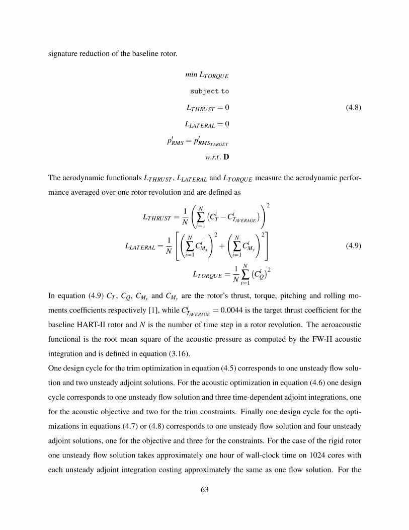
signature reduction of the baseline rotor.
min LTORQUE
subject to
LT HRUST = 0 (4.8)
LLAT ERAL = 0
p′RMS = p′RMSTARGET
w.r.t. D
The aerodynamic functionals LT HRUST , LLAT ERAL and LTORQUE measure the aerodynamic perfor-
mance averaged over one rotor revolution and are defined as
LT HRUST =1N
(N
∑i=1
(Ci
T −CiTAV ERAGE
))2
LLAT ERAL =1N
( N
∑i=1
CiMx
)2
+
(N
∑i=1
CiMy
)2 (4.9)
LTORQUE =1N
N
∑i=1
(Ci
Q)2
In equation (4.9) CT , CQ, CMx and CMy are the rotor’s thrust, torque, pitching and rolling mo-
ments coefficients respectively [1], while CiTAV ERAGE
= 0.0044 is the target thrust coefficient for the
baseline HART-II rotor and N is the number of time step in a rotor revolution. The aeroacoustic
functional is the root mean square of the acoustic pressure as computed by the FW-H acoustic
integration and is defined in equation (3.16).
One design cycle for the trim optimization in equation (4.5) corresponds to one unsteady flow solu-
tion and two unsteady adjoint solutions. For the acoustic optimization in equation (4.6) one design
cycle corresponds to one unsteady flow solution and three time-dependent adjoint integrations, one
for the acoustic objective and two for the trim constraints. Finally one design cycle for the opti-
mizations in equations (4.7) or (4.8) corresponds to one unsteady flow solution and four unsteady
adjoint solutions, one for the objective and three for the constraints. For the case of the rigid rotor
one unsteady flow solution takes approximately one hour of wall-clock time on 1024 cores with
each unsteady adjoint integration costing approximately the same as one flow solution. For the
63

Table 4.2: Operating condition for the HART-II rotor in trimmed forward flightFreestream Mach number (velocity) M∞ = 0.095 (64 kt)Tip Mach Number Mtip = 0.638Advance ratio µ = 0.15Rotational speed Ω = 1041 RPMShaft angle αsha f t = 5.4deg
flexible rotor one unsteady flow solution takes approximately 90 minutes of wall-clock time on
1024 cores with each unsteady adjoint solution costing approximately 45 minutes of wall clock
time. Approximately 650 Gbytes of data are stored to disk during the analysis problem and read in
by the flexible aeroacoustic adjoint procedure. The computational cost of any of the optimizations
in equations (4.6), (4.7) or (4.8) is approaximately 96 hours of wall-clock time on 1024 cores on
the Yellowstone supercomputer at the NCAR-Wyoming Supercomputing Center (NWSC).
The flow conditions for the HART-II rotor are described in Table 4.2 and the simulations are run
for two rotor revolutions using a 2 degree timestep and a computational mesh that consists of ap-
proximately 2.32 million nodes. The aerodynamic functionals in equation (4.9) are accumulated
only over the second revolution to prevent the optimization algorithm from focusing on the initial
transient. The acoustic integration is performed only over the second revolution and the acoustic
objective function is evaluated over the observer time window shown in Figure 3.3(b). For all op-
timizations the observer is stationary and is placed in front of the rotor as shown in Figure 3.2 and
detailed in Table 3.2.
Only shape design variables that affect the outer mold line of the CFD geometry are considered
here. The baseline blade is constructed by stacking 9 airfoils along the span. Each airfoil is pa-
rameterized with 10 Hicks-Henne bump functions [73], 5 for the upper surface and 5 for the lower
surface respectively. Blade twist varies linearly between root and tip, while one collective and
two cyclics allow the trimming of the rotor, for a total of 95 design variables in the vector of
design variables D in equation (4.6), (4.7) and (4.8). For the flexible optimizations no structural
design variables are considered and the optimization design variables affect the aeroelastic loop
only through changes in the aerodynamic forces applied to the structural model.
All the optimizations are driven by the SNOPT sequential quadratic programming algorithm [72]
64

using the unsteady aeroacoustic adjoint capability developed in this work. Convergence results
for the optimization problems are given as a function of nonlinear optimization iterations and of
design cycles. While the number of design cycles is a measure of the optimization wall-clock
time, the number of nonlinear iterations is the number of iterations used by SNOPT to solve the
optimization problem; convergence of the optimization is assessed through feasibility, which is a
measure of the constraint violation, and optimality, which is a measure of the satisfaction of the
Karush - Kuhn - Tucker condition as described in [72].
4.2.1 Rigid HART-II Rotor
Trim Results
The trim optimization problem is described by equation (4.5). The optimization convergence is
shown in Figure 4.7. After 9 nonlinear iterations and 17 design cycles the feasibility and optimality
of the optimization problem are reduced by more than 2 orders of magnitude and the baseline
HART-II rotor is trimmed as further confirmed by thrust and lateral moments time histories shown
in Figure 4.8.
The trimmed HART-II rotor will now serve as the initial design for all subsequent aeroacoustic
optimizations for the rigid rotor.
Aeroacoustic Optimization
As mentioned above the initial design is the trimmed HART-II rotor from the previous section
and the optimization problem is described in equation (4.6). SNOPT convergence is shown in
terms of nonlinear optimization iterations and design cycles in Figure 4.9. After 17 design cycles
the optimization produces a geometry that reduces the Overall Sound Pressure Level of 3.4 dB
while keeping the rotor trimmed as highlighted by the thrust and lateral moments time histories
shown in Figure 4.10. Thickness, loading and total acoustic pressure time histories are shown
in Figure 4.11. Noise minimization is achieved with rather thick airfoils especially at the inboard
sections, as shown in Figure 4.12, while twist and pitch control variables are shown in Table 4.3.
65

(a) Feasibility and optimality of the rigid trim optimization problem as a func-tion of nonlinear optimization iterations
(b) Convergence of the thrust objective function and moment constraint as afunction of design cycles.
Figure 4.7: Convergence of the rigid trim optimization problem
66
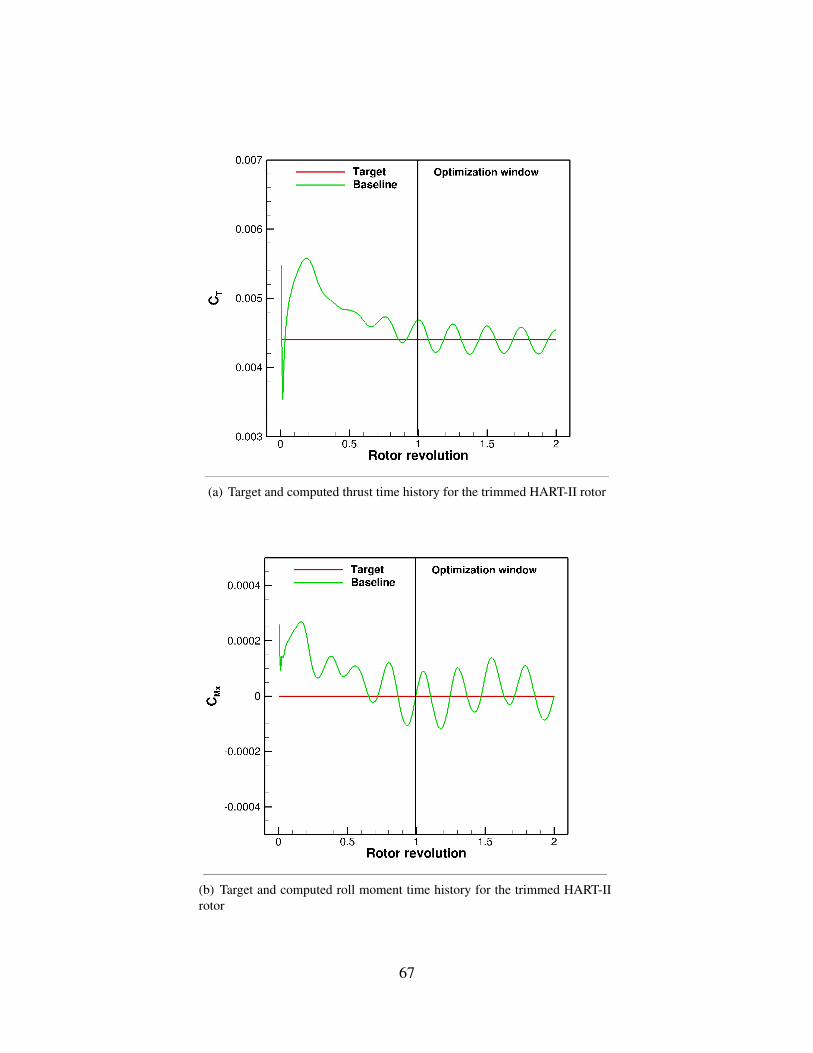
(a) Target and computed thrust time history for the trimmed HART-II rotor
(b) Target and computed roll moment time history for the trimmed HART-IIrotor
67

(c) Target and computed pitch moment time history for the trimmed HART-IIrotor
Figure 4.8: Thrust and moments time histories for the trimmed baseline HART-II rigid rotor
Table 4.3: Twist, collective and cyclics values for the baseline and the aeroacoustically optimizedrigid rotors. All quantities in degrees
Baseline (deg) Aeroacoustic opt. (deg)Root twist 6.0000 6.006Tip twist -2.0000 -2.2513
Collective θ0 -0.7769 -1.0278Cyclic θ1c 0.8954 1.3687Cyclic θ1s -1.7161 -1.7140
68

(a) Feasibility and optimality for the aeroacoustic optimization problem as afunction of nonlinear iterations
(b) Convergence of the aeroacoustic objective function as a function of designcycles.
69

(c) Convergence of the trim constraint as a function of design cycles.
Figure 4.9: Convergence of the aeroacoustic optimization problem for the rigid HART-II rotor
70

(a) Thrust time history for the baseline and the aeroacoustically optimizedtrimmed HART-II rigid rotor
(b) Rolling moment time history for the baseline and the aeroacoustically op-timized trimmed HART-II rigid rotor
71

(c) Pitching moment time history for the baseline and the aeroacousticallyoptimized trimmed HART-II rigid rotor
Figure 4.10: Thrust and moment time histories for the aeroacoustically optimized HART-II rigidrotor
72

Figure 4.11: Thickness, loading and total acoustic pressures at the observer for the aeroacousticallyoptimized rigid rotor
Figure 4.12: Baseline and optimized airfoil shapes for the aeroacoustically optimized rigid rotor
73

Figure 4.13: Baseline and optimized torque time histories for the aeroacoustically optimized rigidrotor showing the performance penalty paid to minimize the acoustic signature.
Since rotor torque is not included in the optimization, the noise reduction achieved here, despite
representing the maximum noise reduction achievable within the current optimization framework,
comes at the expense of rotor performance, as clearly indicated in Figure 4.13. Consequently the
next step is to introduce a torque constraint in the optimization process.
Torque-constrained Aerocoustic Optimization
The initial design for this multidisciplinary aeroacoustic optimization is again the trimmed HART-
II rigid rotor and the optimization problem is described in equation (4.7). After 20 design cycles
the acoustic objective function settles down while attaining the same torque level as the base-
line HART-II rotor, as shown in Figure 4.14(b). The trim constraint feasibility is shown in Fig-
ure 4.14(c) and indicates that the optimized rotor is trimmed, as confirmed by the thrust and lateral
moments time histories shown in Figure 4.15. Contrary to the aeroacoustic optimization, the
74

(a) Feasibility and optimality for the torque-constrained aeroacoustic optimizationproblem as a function of nonlinear iterations
(b) Convergence of the acoustic objective function and the torque constraint as afunction of design cycles.
75
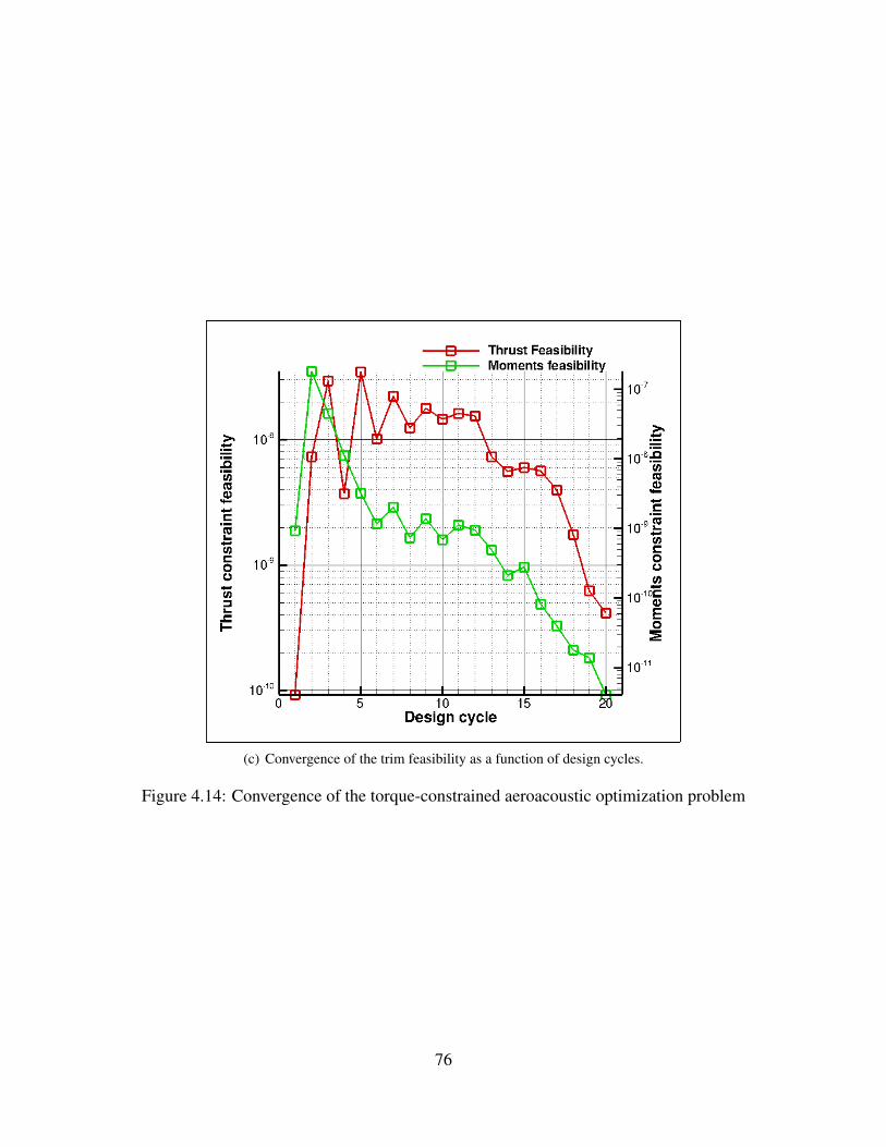
(c) Convergence of the trim feasibility as a function of design cycles.
Figure 4.14: Convergence of the torque-constrained aeroacoustic optimization problem
76

(a) Thrust time history for the baseline and torque-constrained aeroacoustically op-timized trimmed HART-II rigid rotor
(b) Rolling moment time history for the baseline and the torque-constrained aeroa-coustically optimized trimmed HART-II rigid rotor
77

(c) Pitching moment time history for the baseline and the torque-constrained aeroa-coustically optimized trimmed HART-II rigid rotor
Figure 4.15: Thrust and moment time histories for baseline and the torque-constrained aeroacous-tically optimized trimmed HART-II rigid rotor
78

Figure 4.16: Baseline and optimized torque time histories for the torque-constrained aeroacousti-cally optimized rigid rotor.
torque level for the torque-constrained aeroacoustically optimized rigid rotor is the same as that of
the baseline HART-II rigid rotor as shown in Figure 4.16. Thickness, loading and total acoustic
pressure time histories at the observer are shown in Figure 4.17. The optimized rotor is 1.7 dB
quieter in terms of Overall Sound Pressure Level. A comparison between the baseline and opti-
mized airfoils is shown in Figure 4.18 where it can be seen that, as in the case of the aeroacoustic
optimization in the previous section, the optimized shapes tend to be thicker at the inboard stations
and thinner at the outboard ones. Twist and pitch control variables are given in Table 4.4.
Previous noise mitigation studies [8] have shown that optimizing for one observer location can
result in higher noise levels at different observer locations. A directivity study for the optimized
rotor reveals that the current design is capable of reducing noise at in-plane observer locations that
have not been targeted by the optimization as shown for two different observers placed at ψ = 135
and ψ = 315 degrees as shown in Figure 4.19.
79

Figure 4.17: Thickness, loading and total acoustic pressures at the observer for the torque - con-strained aeroacoustically optimized rigid rotor
Figure 4.18: Torque-constrained aeroacoustically optimized airfoil shapes
80

(a) Baseline and optimized total acoustic pressure time history at ψ = 135degrees
(b) Baseline and optimized total acoustic pressure time history at ψ = 315degrees
Figure 4.19: Directivity study for the baseline and optimized rigid rotor geometries
81
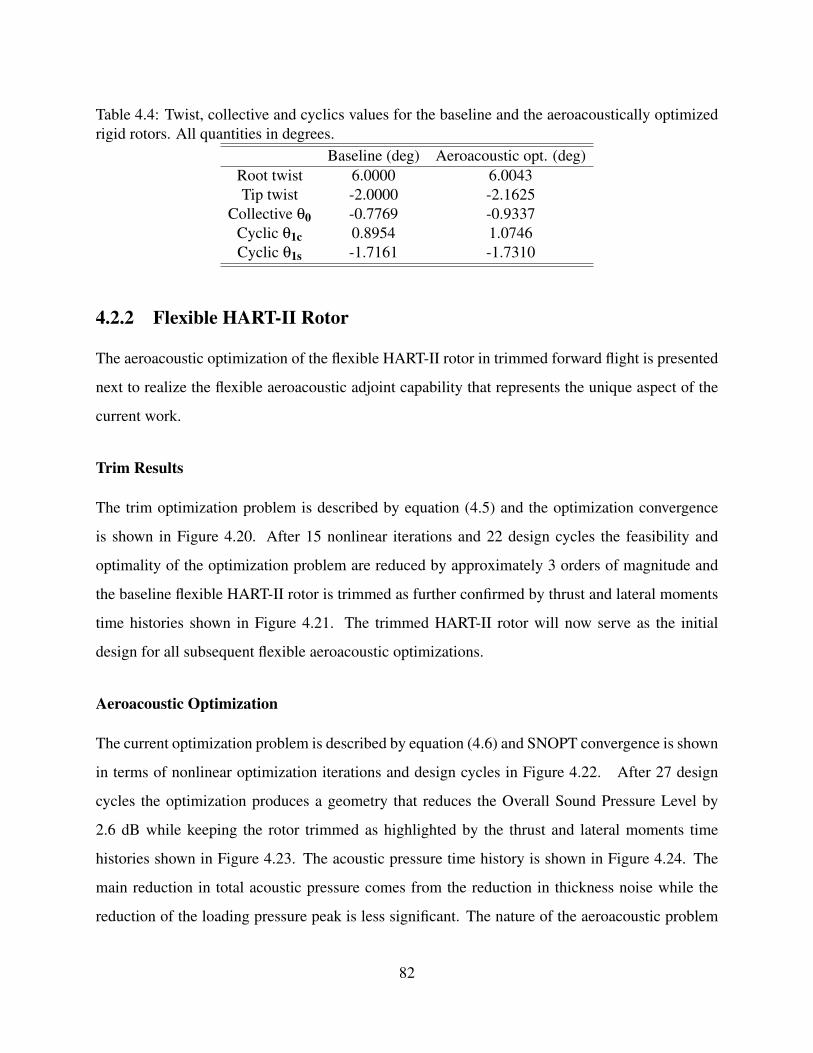
Table 4.4: Twist, collective and cyclics values for the baseline and the aeroacoustically optimizedrigid rotors. All quantities in degrees.
Baseline (deg) Aeroacoustic opt. (deg)Root twist 6.0000 6.0043Tip twist -2.0000 -2.1625
Collective θ0 -0.7769 -0.9337Cyclic θ1c 0.8954 1.0746Cyclic θ1s -1.7161 -1.7310
4.2.2 Flexible HART-II Rotor
The aeroacoustic optimization of the flexible HART-II rotor in trimmed forward flight is presented
next to realize the flexible aeroacoustic adjoint capability that represents the unique aspect of the
current work.
Trim Results
The trim optimization problem is described by equation (4.5) and the optimization convergence
is shown in Figure 4.20. After 15 nonlinear iterations and 22 design cycles the feasibility and
optimality of the optimization problem are reduced by approximately 3 orders of magnitude and
the baseline flexible HART-II rotor is trimmed as further confirmed by thrust and lateral moments
time histories shown in Figure 4.21. The trimmed HART-II rotor will now serve as the initial
design for all subsequent flexible aeroacoustic optimizations.
Aeroacoustic Optimization
The current optimization problem is described by equation (4.6) and SNOPT convergence is shown
in terms of nonlinear optimization iterations and design cycles in Figure 4.22. After 27 design
cycles the optimization produces a geometry that reduces the Overall Sound Pressure Level by
2.6 dB while keeping the rotor trimmed as highlighted by the thrust and lateral moments time
histories shown in Figure 4.23. The acoustic pressure time history is shown in Figure 4.24. The
main reduction in total acoustic pressure comes from the reduction in thickness noise while the
reduction of the loading pressure peak is less significant. The nature of the aeroacoustic problem
82

(a) Feasibility and optimality of the trim problem as a function of nonlinearoptimization iterations
(b) Convergence of the thrust objective function and moment constraint as afunction of design cycles.
Figure 4.20: Convergence of the trim optimization problem for the flexible HART-II rotor
83

Figure 4.21: Thrust and moments time histories for the baseline HART-II flexible rotor
dictates the optimization behavior: for in-plane noise problems thickness noise is the dominant
source of noise [74], hence SNOPT chooses a trimmed geometry that minimizes thickness noise.
The noise minimization is achieved with rather thick airfoils especially at the inboard sections, as
shown in Figure 4.25. Blade root cap shape considerations dictate the shape of the most inboard
airfoil at the first spanwise station: the blade cap is built as a surface of revolution that joins
the upper and lower surface of the blade, the design variables for the root airfoil needed to be
bounded more than the design variables for the other airfoils to guarantee a reasonable blade root
cap, resulting in the first airfoil shown in Figure 4.25. Twist and pitch design variables are shown
in Table 4.5. Since rotor torque is not included in the optimization, the noise reduction achieved
here, despite representing the maximum noise reduction achievable within the current optimization
framework, comes at the expense of rotor performance, as clearly indicated in Figure 4.26.
The optimization described by equation (4.7) and discussed in the next section adresses this issue
by minimizing the required torque while constraining the acoustic signature to a lower noise level
than the baseline rotor.
84

(a) Feasibility and optimality for the aeroacoustic optimization problem as a func-tion of nonlinear iterations
(b) Convergence of the aeroacoustic objective function as a function of design cy-cles.
85

(c) Convergence of the trim constraint as a function of design cycles.
Figure 4.22: Convergence of the flexible aeroacoustic optimization problem
Table 4.5: Twist, collective and cyclics values for the baseline and the aeroacoustically optimizedflexible rotors. All quantities in degrees.
Baseline (deg) Aeroacoustic opt. (deg)Root twist 6.0000 6.0947Tip twist -2.0000 -2.7574
Collective θ0 -0.4986 -1.1146Cyclic θ1c 1.3678 1.5074Cyclic θ1s -2.5530 -2.8053
86

Figure 4.23: Thrust and moments time histories for the baseline and optimized flexible HART-IIrotors
Observer time []
Th
ick
ne
ss
pre
ss
[]
115 120 125 130 135 140 145 150 155 160
0.0008
0.0004
0
Observer time []
Lo
ad
ing
pre
ss
[]
115 120 125 130 135 140 145 150 155 160
0.0002
0.0001
0
Observer time []
Ac
ou
sti
c p
res
s [
]
115 120 125 130 135 140 145 150 155 160
0.0008
0.0004
0
Figure 4.24: Thickness, loading and total acoustic pressures at the observer for the baseline (red)and the aeroacoustically optimized (green) flexible rotors
87

Figure 4.25: Baseline (red) and optimized (green) airfoil shapes for the aeroacoustically optimizedflexible rotors
Figure 4.26: Torque time history for the baseline and aeroacoustically optimized flexible rotorsshowing the performance penalty paid to minimize the acoustic signature.
88

Table 4.6: Twist, collective and cyclics values for the baseline and the aeroacoustically optimizedflexible rotors. All quantities in degrees.
Baseline (deg) Aeroacoustic opt. (deg)Root twist 6.0000 5.9996Tip twist -2.0000 -2.0022
Collective θ0 -0.4986 -0.5028Cyclic θ1c 1.3678 1.3790Cyclic θ1s -2.5530 -2.6021
Acoustically-constrained Torque Minimization
The minimization problem for the optimization presented in this section is described in equation
(4.8). In as few as 5 nonlinear iterations feasibility is reduced by more than 2 orders of mag-
nitude while optimality is reduced by approximately 9 orders of magnitude, as shown in Figure
4.27(a). After 10 design cycles the acoustic constraint is satisfied resulting in a rotor with a 2dB
OSPL reduction compared to the baseline, while the required torque is reduced by 2.5% as shown
in Figure 4.27(b). Satisfaction of the trim constraint is shown in Figure 4.27(c) and confirmed by
the thrust and lateral moment time histories shown in Figure 4.28. A comparison of the torque
time histories is shown in Figure 4.29 highlighting the 2.5% torque reduction achieved for this
optimization. The thickness, loading and total acoustic pressure time histories are shown in Fig-
ure 4.30. The thickness acoustic pressure is essentially the same between the current optimization
and the one from the previous section, suggesting that the two minimizations exploit the same
noise reduction mechanism, while loading pressure reduction for the current optimization is sig-
nificantly lower. A comparison of the airfoil shapes for the baseline and the two optimized rotors
is shown in Figure 4.31 highlighting that the acoustically constrained torque minimization results
in more conventional blade shapes at the inboard sections while recovering the same airfoils of
the aeroacoustic optimization at the outboard sections. Twist and pitch control parameters for this
optimization are shown in Table 4.6.
As for the case of the rigid rotor, a directivity study for the baseline and the optimized flexible rotors
is performed and reveals that the current design is capable of reducing noise at in-plane observer
89

(a) Feasibility and optimality for the torque-constrained aeroacoustic optimizationproblem as a function of nonlinear iterations
(b) Convergence of the acoustic objective function and the torque constraint as afunction of design cycles. 90

(c) Convergence of the trim feasibility as a function of design cycles.
Figure 4.27: Convergence of the acoustically constrained torque optimization of the flexibleHART-II rotor
91

Figure 4.28: Thrust and moments time histories for the baseline, the aeroacoustic optimized andthe acoustically constrained torque optimized flexible rotors
locations that have not been targeted by the optimization, as shown in Figures 4.32 and 4.33. Figure
4.32 shows the total acoustic pressure for the baseline and the optimized rotors at the same radial
location used during the optimization but for different azimuthal locations, while Figure 4.33 shows
the acoustic pressure for the same azimuthal location targeted by the optimization but at different
radial distances. In both cases the noise signature for the optimized rotor is smaller than that of the
baseline rotor. As mentioned before, thickness acoustic pressure is the dominant source of noise for
the current aeroacoustic problem and the solid wall acoustic integration implies that the thickness
integral in the FW-H equation (3.12) depends only on geometrical and kinematic parameters of the
rotor, hence justifying the results of the current directivity study.
Validation of Optimization Results over Multiple Rotor Revolutions
In this section we investigate the behavior of the baseline and the optimized flexible rotors from
the previous sections when their performance is evaluated over multiple rotor revolutions. While
the previous computations have been run for only 2 rotor revolutions, the current simulations have
92

Figure 4.29: Torque time histories for the baseline, the aeroacoustic optimized and the acousticallyconstrained torque optimized flexible rotors
been run for four rotor revolutions and the aerodynamic objective functions are accumulated over
the last 3 revolutions. The acoustic objective function is evaluated over the same observer time
window as in the previous sections. The geometry and the control variables are the same as those
from the previous sections.
As expected, since the rotor does not achieve a fully periodic state within 2 revolutions, the rotors
are now untrimmed for the subsequent revolutions, however the trim constraint is violated by the
same amount by the three rotors, as shown in Figure 4.34, allowing for a meaningful comparison
of the acoustic signature and of the required torque. The observer acoustic pressure time histories,
shown in Figure 4.35, confirm the results from the previous sections: the aeroacoustically opti-
mized rotor yields the most significant noise signature reduction when compared to the baseline
rotor with a noise reduction of 2.7 dB OSPL at the observer, however the required torque is sig-
nificantly increased, as shown in Figure 4.36. The acoustically constrained torque optimized rotor
yields 2.9% reduction in required torque with a 1.9 dB OSPL reduction in noise signature.
These results show that even if the optimizations targeted only the second rotor revolution, they
93

Observer time []
Th
ick
ne
ss
pre
ss
[]
115 120 125 130 135 140 145 150 155 160
0.0008
0.0004
0
Observer time []
Lo
ad
ing
pre
ss
[]
115 120 125 130 135 140 145 150 155 160
0.0002
0.0001
0
Observer time []
Ac
ou
sti
c p
res
s [
]
115 120 125 130 135 140 145 150 155 160
0.0008
0.0004
0
Figure 4.30: Thickness, loading and total acoustic pressures at the observer for the baseline (red),the acoustically optimized (green) and the acoustically constrained torque optimized (blue) flexiblerotors.
Figure 4.31: Acoustically constrained torque optimized blade shapes
94

(a) Baseline and optimized total acoustic time history at ψ = 135 degrees
(b) Baseline and optimized total acoustic time history at ψ = 315 degrees
Figure 4.32: Directivity study for the baseline and optimized flexible geometries: radial distance2R, different azimuthal locations
95

(a) Baseline and optimized total acoustic time history at 50R
(b) Baseline and optimized total acoustic time history at 100R
Figure 4.33: Directivity study for the baseline and optimized flexible geometries: Azimuth ψ= 180degs, different radial locations
96

Figure 4.34: Thrust and moments time histories for the baseline, the aeroacoustic optimized andthe acoustically constrained torque optimized flexible rotors over 4 rotor revolutions
Figure 4.35: Thickness, loading and total acoustic pressures at the observer for the baseline andthe two optimized flexible rotors for the multiple revolutions case.
97

Figure 4.36: Torque time histories for the baseline, the aeroacoustic optimized and the acousticallyconstrained torque optimized flexible rotors over 4 rotor revolutions
still have been able to improve rotor performance over multiple rotor revolutions. The resulting
optimal rotors can be used as intial guesses for more expensive optimizations that target multiple
rotor revolutions.
98

Chapter 5
Conclusions and Future Work
This thesis has presented the development and application of an adjoint-based method for aeroa-
coustics, with a particular emphasis on rotorcraft design problems. The aeroacoustic adjoint tech-
nique has been first developed for two-dimensional applications and it has been applied to the noise
minimization of an airfoil in blade-vortex interaction. The two-dimensional formulation has then
been extended to include three-dimensional effects. The three-dimensional aeroacoustic adjoint ca-
pability has been first applied to the gradient-based noise minimization of a rigid rotor in forward
flight. Subsequently, blade flexibility effects have been included in the optimization to realize
a unique and unprecedented multidisciplinary adjoint-based optimization capability that encom-
passes the three disciplines of aerodynamics, structural mechanics and aeroacoustics. By yielding
optimal rotors characterized by superior aeroacoustic and aerodynamic performance, these opti-
mizations show that the multidisciplinary adjoint techniques developed in this work can be used
to efficiently solve the high-fidelity, large-scale design optimization problems often encountered
in rotorcraft design, without the severe design space limitations typical of earlier optimization at-
tempts.
Possible future development for the work presented in this thesis should focus on further advanc-
ing the state-of-the-art in both rotorcraft design optimization and adjoint-based optimization tech-
niques. To advance the state-of-the-art in rotorcraft design, future research activities should focus
on:
• Optimization on finer meshes targeting multiple rotor revolutions: In this thesis no at-
99

tempt has been made at quantifying the effect of spatial and temporal mesh resolution on the
aerodynamic and aeroacoustic performance of the rotor. A systematic investigation of the
effect of discretization errors on the predicted performance of the rotor, similar to the grid-
convergence studies in [75], will allow to identify the optimal spatial and temporal mesh
resolution to be employed in the optimization procedure. Furthermore, in Chapter 4, Section
4.2.2, it has been shown that the forces acting on the rotor have not yet reached a periodic
state after two rotor revolutions. To avoid concentrating the optimization efforts on transient
flow conditions of little interest to the rotorcraft designer, more rotor revolutions need to be
included in the simulation and the optimization objective functionals should be evaluated
only after a periodic state has been reached. However, in Chapter 4, Section 4.2.2 it has also
been shown that the optimization results presented in this thesis can be used as initial designs
for lengthier, more expensive optimizations that target multiple rotor revolutions.
• Including higher fidelity structural models: while the Hodges-Dowell beam model em-
ployed in this work is in widespread use in the rotorcraft industry, the use of a higher fidelity
structural model based on bricks and shell elements will allow for a more accurate descrip-
tion of the geometry and the structural dynamics of the blade. Furthermore, the new struc-
tural model will allow to easily update the blade structural properties in response to major
changes in the blade shape and to include structural design variables and objectives in the
multidisciplinary optimization process.
• Including nonlinear flow effects in the aeroacoustic prediction: to allow for the aeroa-
coustic optimization of rotors characterized by high tip Mach numbers, the quadrupole noise
term should be included in the acoustic analogy. The most common approach to account for
quadrupole noise in the aeroacoustic prediction is to perform the acoustic integration on an
off-body, permeable, integration surface provided that the flowfield between the rotor and
the integration surface is sufficiently resolved. Thanks to the choice of the acoustic formula-
tion implemented in this work, the only action required to include quadrupole noise effects
in the current optimization framework is the identification of a suitable off-body integration
surface.
100

• Investigating multiple local minima: as stated before, gradient-based optimization algo-
rithms seek a saddle point of the Lagrangian function associated with the optimization prob-
lem. In the case of a multimodal design space, typical of large-scale problems, gradient-
based optimization algorithms can potentially be trapped in a local minimum for the opti-
mization problem. As proposed by Lyu et al. [76], the multimodality of the design space
should be investigated by starting the optimization from random initial geometries. If the ro-
torcraft design space is found to be multimodal, a hybrid optimization strategy that combines
the efficiency of gradient based optimization algorithms with the intrinsic global nature of
evolutionary methods should be pursued. Previous work [16, 77] in this area has focused
on enhancing metamodeling techniques, Kriging or response surface methods, with gradient
information computed with the adjoint approach.
• Investigating multipoint design optimization: Single point design optimizations such as
the ones presented in this work yield optimal geometries for which the performance deterio-
rate quickly at off design conditions. A more robust approach to rotorcraft design would be
to perform a multipoint optimization where different design conditions are targeted simul-
taneously. In the context of helicopter design it would be natural to target both hover and
forward flight to optimize the aerodynamic and the aeroacoustic performance of the vehi-
cle. Furthermore, adopting a higher-fidelity structural model and including structural design
variables and objectives in the optimization process could allow the multipoint optimization
to also target a maneuver condition realizing a fully automated design optimization process.
Strategies to develop discrete adjoint sensitivities are now fairly well understood and future work
on adjoint-based optimizaton should focus on:
• Evaluating algorithms for the solution of linear systems with multiple right hand sides:
The use of sequential quadratic programming algorithms for the solution of the large-scale
design optimization problems treated in this work requires the full sensitivity vector of the
objective and the constraint of the optimization problem. The adjoint method presented in
this work provides an efficient way of computing sensitivity of one functional with respect
to a set of design variables. When multiple functionals are present, the adjoint system needs
101

to be solved multiple times as its right hand side depends on the particular functional be-
ing considered, as shown in equation (3.29). Hence, algorithms that allow for the efficient
solution of linear systems with multiple right-hand-sides should be considered in the future
to improve the performance of the current optimization framework. By accessing the co-
efficient matrix and performing all the necessary floating point operations only once for all
the right hand sides, the solution of linear systems with multiple right hand sides should be
well suited for execution on emerging computer architectures. While Jacobi-like iterative
schemes can be trivially extended to the simultaneous solution of mulitiple linear systems,
the generalization of Krylov-based methods to the multiple right-hand-side case is more in-
volved [78]. Finally, the efficient solution of linear systems with multiple right hand sides
could allow for the evaluation of the exact Hessian matrix of the optimization problem, sig-
nificantly improving the performance of the optimization algorithm employed.
• Investigating the effect of gradient accuracy on the performance of the optimization
algorithms: since any gradient-based optimization algorithm uses gradient information to
identify a local minimum for the objective function, the accuracy of the gradient is expected
to significantly affect the performance of the optimization algorithm. Previous studies have
investigated the effect that approximations to the adjoint linearization have on the optimiza-
tion process [79]. The tangent and adjoint linearizations presented in this work are verified
to machine precision provided that the nonlinear flow solution is completely converged. For
realistic applications converging the nonlinear residuals to zero is unrealistic at best. In a
realistic scenario the nonlinear residuals are only partially converged, resulting in inaccurate
gradient computations. By slightly modifying the derivation of the adjoint equations pre-
sented in this thesis, different strategies can be devised to account for errors resulting from
partial convergence of the nonlinear flow problem. These strategies should be thoroughly in-
vestigated to understand and address the effect that partial convergence of the flow solution
has on the optimization process.
102

References
[1] W. Johnson, Rotorcraft Aeromechanics. Cambridge University Press, 2013.
[2] W. R. Johnson, “Rotorcraft Aerodynamics Models for a Comprehensive Analysis,” in 54thAmerican Helicopter Society Annual Forum and Technology Display, Washington, DC, May1998.
[3] A. M. Wissink, J. Sitaraman, V. Sankaran, M. D. J., and P. T. H., “A Multi-Code Python BasedInfrastructure for Overset CFD with Adaptive Cartesian Grids,” in 46th AIAA AerospaceSciences Meeting, Reno, NV, 2008, AIAA Paper 2008–0927.
[4] M. Costes, T. Renaud, and B. Rodriguez, “Rotorcraft Simulations: a Challenge for CFD,” In-ternational Journal of Computational Fluid Dynamics, vol. 26, no. 6-8, pp. 383–405, October2012.
[5] Y. H. Yu, C. Tung, B. van der Wall, H.-J. Pausder, C. Burley, T. Brooks, P. Beaumier, Y. Del-rieux, E. Mercker, and K. Pengel, “The HART-II Test: Rotor Wakes and Aeroacoustics withHigher-Harmonic Pitch Control (HHC) Inputs -The Joint German/French/Dutch/US Project-,” in 58th American Helicopter Society Annual Forum, Montreal, Canada, June 11–13 2002.
[6] B. Edwards and C. Cox, “Revolutionary Concepts for Helicopter Noise Reduction -S.I.L.E.N.T Program,” NASA, Tech. Rep. CR-2002-211650, May 2002.
[7] Y. H. Yu, “Rotor Blade Vortex Interaction Noise,” Progress in Aerospace Sciences, vol. 36,pp. 97–115, 2000.
[8] B. W. Sim, R. D. Janakiram, N. L. Barbely, and E. Solis, “Reduced In-Plane, Low Fre-quency Noise of an Active Flap Rotor,” in American Helicopter Society 65th Annual Forum,Grapevine, TX, May 2009.
[9] S. Chae, K. Yee, C. Yang, T. Aoyama, S. Jeong, and S. Obayashi, “Helicopter Rotor ShapeOptimization for the Improvement of Aeroacoustic Performance in Hover,” Journal of Air-craft, vol. 47, no. 5, pp. 1770–1783, Semptember–October 2010.
[10] B. G. Marinus, M. Roger, V. den Braembussche, and W. Bosschaerts, “Multidisciplinary Op-timization of Propeller Blades: Focus on Acoustic Results,” in 47th AIAA/ASME/SAE/ASEEJoint Propulsion Conference and Exhibit, 2011, AIAA Paper 2011–2801.
103

[11] J. D. Baeder, “Euler Solutions to Nonlinear Acoustics of Non-Lifting Hovering RotorBlades,” NASA, Tech. Rep. TM-103837, February 1991.
[12] J. Bain, “Computational Comparison Between FW-H and Direct Acoustic Predictions,” in72nd Forum and Technology Display of the American Helicopter Society, 2016, AHS Paper2016–185.
[13] F. Farassat and G. P. Succi, “The Prediction of Helicopter Discrete Frequency Noise,” Vertica,vol. 7-4, pp. 309–320, 1983.
[14] K. S. Brentner and F. Farassat, “Modeling Aerodynamically Generated Sound of HelicopterRotors,” Progress in aerospace sciences, vol. 39, pp. 83–120, 2003.
[15] A. J. Keane and B. N. Prasanth, Computational Approaches for Aerospace Desing. Wiley,2005.
[16] A. Forrester, A. Sobester, and A. Keane, Engineering Design via Surrogate Modelling: APractical Guide. Wiley, 2008.
[17] B. R. Jones, C. W. A., and A. S. Lyrintzis, “Aerodynamic and Aeroacoustic Optimizationof Rotorcraft Airfoils via a Parallel Genetic Algorithm,” Journal of Aircraft, vol. 37-6, pp.1088–1096, 2000.
[18] B. G. Marinus, M. Roger, V. den Braembussche, and W. Bosschaerts, “Multidisciplinary Op-timization of Propeller Blades: Focus on Acoustic Results,” in 47th AIAA/ASME/SAE/ASEEJoint Propulsion Conference and Exhibit, 2011, AIAA Paper 2011–2801.
[19] J. C. Vassberg and A. Jameson, “Influence of Shape Parameterization On Aerodynamic ShapeOptimization,” in VKI Lecture Series on Aerodynamic Drag Prediction and Reduction, vonKarman Institute of Fluid Dynamics, Rhode St Genese, Belgium, 2014.
[20] J. L. Walsh, G. J. Bingham, and M. F. Riley, “Optimization Method Applied to the Aerody-namic Design of Helicopter Rotor Blades,” Journal of the American Helicopter Society, vol.32-4, pp. 39–44, 1987.
[21] J. Zibi, G. Defresen, and M. Costes, “A Numerical Procedure for Aerodynamic Optimizationof Helicopter Rotor Blades,” in Proceedings of the 18th European Rotorcraft Forum, 1992.
[22] N. Jorge and W. S. J., Numerical Optimization. Springer, 2006.
[23] A. Jameson and L. Martinelli, “Aerodynamic Shape Optimization Techniques Based onControl Theory,” in Computational Mathematics Driven by Industrial Problems, ser. LectureNotes in Mathematics, R. Burkard, A. Jameson, G. Strang, P. Deuflhard, J.-L. Lions,V. Capasso, J. Periaux, and H. Engl, Eds. Springer Berlin Heidelberg, 2000, vol. 1739, pp.151–221. [Online]. Available: http://dx.doi.org/10.1007/BFb0103920
[24] Z. Lyu, K. W. Kenway, and J. R. R. A. Martins, “Aerodynamic Shape Optimization Inves-tigation of the Common Research Model Wing Benchmark,” AIAA Journal, vol. 53-4, pp.968–985, 2015.
104

[25] E. Nielsen and W. Anderson, “Recent Improvements in Aerodynamic Design Optimizationon Unstructured Meshes,” AIAA Journal, vol. 40, no. 6, pp. 1155–1163, June 2002.
[26] S. Kim, A. J., and A. Jameson, “Multi-Element High-Lift Configuration Design OptimizationUsing Viscous Continuous Adjoint Method,” Journal of Aircraft, vol. 41, no. 5, pp. 1082–1097, 2004.
[27] F. Bisson and S. Nadarajah, “Adjoint-Based Aerodynamic Optimization of Benchmark Prob-lems,” in 53rd AIAA Aerospace Sciences Meeting, Kissimmee, Fl, January 2015, AIAA Paper2015-1948.
[28] C. Lee, K. Telidetzki, H. Buckley, H. Gagnon, and D. W. Zingg, “Aerodynamic Shape Opti-mization of Benchmark Problems Using Jetstream,” in 53rd AIAA Aerospace Sciences Meet-ing, Kissimmee, Fl, January 2015, AIAA Paper 2015-0262.
[29] M. Giles, M. Duta, J. Muller, and N. A. Pierce, “Algorithm Developments for Discrete Ad-joint Methods,” AIAA Journal, vol. 41, no. 2, pp. 198–205, February 2003.
[30] A. Jameson and J. Vassberg, “Computational Fluid Dynamics for Aerodynamic Design: ItsCurrent and Future Impact,” in Proceedings of the 39th Aerospace Sciences Meeting andExhibit, Reno NV, 2001, AIAA Paper 2001–0538.
[31] A. Jameson, “Aerodynamic Shape Optimization using the Adjoint Method,” in VKI LectureSeries on Aerodynamic Drag Prediction and Reduction, von Karman Institute of Fluid Dy-namics, Rhode St Genese, Belgium, 2003.
[32] D. J. Mavriplis, “Solution of the Unsteady Discrete Adjoint for Three-Dimensional Problemson Dynamically Deforming Unstructured Meshes,” in Proceedings of the 46th AerospaceSciences Meeting and Exhibit, Reno NV, 2008, AIAA Paper 2008–0727.
[33] E. Nielsen and B. Diskin, “Discrete Adjoint-Based Design for Unsteady Turbulent Flowson Dynamic Overset Unstructured Grids,” in 50th AIAA Aerospace Sciences Meeting andExhibit, Nashville, TN, January 9-12 2012, aIAA Paper 2012–0554.
[34] E. Nielsen, B. Diskin, and N. K. Yamaleev, “Discrete Adjoint-Based Design Optimization ofUnsteady Turbulent Flows on Dynamic Unstructured Grids,” AIAA Journal, vol. 48, no. 6,pp. 1195–1206, June 2010.
[35] K. Mani and D. J. Mavriplis, “Unsteady Discrete Adjoint Formulation for Two-DimensionalFlow Problems with Deforming Meshes,” AIAA Journal, vol. 46, no. 6, pp. 1351–1364, June2008.
[36] S. W. Lee and O. J. Kwon, “Aerodynamic Shape Optimization of Hovering Rotor Blades inTransonic Flow Using Unstructured Meshes,” AIAA Journal, vol. 44, no. 8, pp. 1816–1825,August 2006.
[37] J. R. R. A. Martins and A. B. Lambe, “Multidisciplinary Design Optimization: A Survey ofArchitectures,” AIAA Journal, vol. 51, pp. 2049–2075, 2013.
105

[38] A. Mishra, K. Mani, D. J. Mavriplis, and J. Sitaraman, “Helicopter Rotor Design usingAdjoint-based Optimization in a Coupled CFD-CSD Framework,” in 69th American Heli-copter Society Annual Forum, Phoenix, AZ, May 21–23 2013.
[39] M. Rumpfkeil and D. Zingg, “The Optimal Control of Unsteady Flows With a Discrete Ad-joint Method,” Journal of Optimization and Engineering, vol. 11, no. 1, pp. 5–22, 2010.
[40] T. D. Economon, F. Palacios, and J. J. Alonso, “A Coupled-Adjoint Method for Aerody-namic and Aeroacoustic Optimization,” in 14th AIAA/ISSM Multidisciplinary Analysis andOptimization Conference, 2012, AIAA Paper 2012–5598.
[41] D. J. Mavriplis, “Unstructured-Mesh Discretizations and Solvers for Computational Aerody-namics,” AIAA Journal, vol. 46-6, pp. 1281–1298, June 2008.
[42] A. Jameson, “Time Dependent Calculations Using Multigrid, with Applications to UnsteadyFlows Past Airfoils and Wings,” in Proceedings of the 10th Computational AerodynamicsConference, Honolulu HI, 1991, AIAA Paper 1991–1596.
[43] Y. Saad, Iterative Methods for Sparse Linear Systems. SIAM, 2003, 2nd edition.
[44] B. M. Kulfan, “Universal Parametric Geometry Representation Method,” Journal of Aircraft,vol. 45-1, pp. 142–158, 2008.
[45] H. C. Yee, N. D. Sandham, and M. J. Djomehri, “Low-Dissipative High-Order Shock-Capturing Methods Using Characteristic-Based Filters,” Journal of Computational Physics,vol. 150, pp. 199–238, 1999.
[46] J. E. Ffowcs Williams and D. L. Hawkings, “Sound Generation by Turbulence and Surfacesin Arbitrary Motion,” Philosophical Transactions of the Royal Society of London. Series A,Mathematical and Physical Sciences, vol. 264-1151, pp. 321–342, May 1969.
[47] P. di Francescantonio, “A New Boundary Integral Formulation for the Prediction of SoundRadiation,” Vertica, vol. 7-4, pp. 309–320, 1983.
[48] D. P. Lockard, “An Efficient Two-Dimensional Implementation of the Ffowcs Williams andHawkings Equation,” Journal of Sound and Vibration, vol. 224-4, pp. 897–911, 2000.
[49] W. H. Press, S. A. Teukolsky, W. T. Vetterling, and B. P. Flannery, Numerical Recipes inFORTRAN. Cambridge University Press, 1992.
[50] D. G. Crighton, A. P. Dowling, and J. E. Ffowcs Willliams, Modern Methods in AnalyticalAcoustics. Springer-Verlag, 1992.
[51] M. Rumpfkeil, “Airfoil Optimization for Unsteady Flows With Application to High-LiftNoise Reduction,” Ph.D. dissertation, University of Toronto, 2008.
[52] J. N. Lyness and C. B. Moler, “Numerical Differentiation of Analytic Function,” SIAM Jour-nal of Numerical Analysis, vol. 4-2, pp. 202–210, 1967.
106

[53] J. R. R. A. S. P. Martins and J. J. Alonso, “The Complex-Step Derivative Approximation,”ACM Transactions on Mathematical Software, vol. 29-3, pp. 245–262, 2003.
[54] D. J. Mavriplis, “Discrete Adjoint-Based Approach for Optimization Problems on Three-Dimensional Unstructured Meshes,” AIAA Journal, vol. 45-4, pp. 741–750, April 2007.
[55] D. J. Mavriplis and K. Mani, “Unstructured Mesh Solution Technique Using the NSU3DSolver,” in Proceedings of the 52nd AIAA Aerospace Sciences Conference, National Harbor,MD, 2014, AIAA Paper 2014–0081.
[56] K. Mani and D. J. Mavriplis, “Geometry Optimization in Three-Dimensional Unsteady FlowProblems using the Discrete Adjoint,” in 51st AIAA Aerospace Sciences Meeting, Grapevine,TX, January 2013, AIAA Paper 2013-0662.
[57] P. R. Spalart and S. R. Allmaras, “A One-equation Turbulence Model for AerodynamicFlows,” La Recherche Aerospatiale, vol. 1, pp. 5–21, 1994.
[58] D. J. Mavriplis, “Multigrid Strategies for Viscous Flow Solvers on Anisotropic UnstructuredMeshes,” Journal of Computational Physics, vol. 145, no. 1, pp. 141–165, Sep. 1998.
[59] D. H. Hodges and E. H. Dowell, “Nonlinear Equations Of Motion For The Elastic BendingAnd Torsion of Twisted Nonuniform Rotor Blades,” NASA, Tech. Rep. TN-D-7818, Decem-ber 1974.
[60] D. J. Mavriplis, Z. Yang, and M. Long, “Results using NSU3D for the first AeroelasticPrediction Workshop,” in Proceedings of the 51st Aerospace Sciences Meeting and Exhibit,Grapevine TX, 2013, AIAA Paper 2013–0786.
[61] D. M. Schuster, P. Chwalowski, J. Heeg, and C. D. Wieseman, “Summary of Data and Find-ings from the First Aeroelastic Prediction Workshop,” in Seventh International Conferenceon Computational Fluid Dynamics (ICCFD7). Big Island, HI: ICCFD, July 9-13 2012.
[62] A. Mishra, K. Mani, D. J. Mavriplis, and J. Sitaraman, “Time-dependent Adjoint-basedAerodynamic Shape Optimization Applied to Helicopter Rotors,” Journal of ComputationalPhysics, vol. 292, no. 1, pp. 253–271, 2015, doi:10.1016/j.jcp.2015.03.010.
[63] I. Chopra and G. Bir, “University of Maryland Advanced Rotor Code: UMARC,” in Ameri-can Helicopter Society Aeromechanics Specialists Conference, San Franscisco, CA, January1994.
[64] Heckmann, M. A. Otter, S. Dietz, and J. D. Lopez, “The DLR FlexibleBodies Library toModel Large Motions of Beams and of Flexible Bodies Exported from Finite Element Pro-grams,” in Modelica, September 4–5 2006.
[65] A. A. Kumar, S. R. Vishwamurthy, and R. Ganguli, “Correlation of Helicopter Rotor Aeroe-lastic Response with HART-II Wind Tunnel Test Data,” Aircraft Engineering and AerospaceTechnology: An International Journal, vol. 82, no. 4, pp. 237–248, 2010.
107

[66] Z. Yang and D. J. Mavriplis, “A Mesh Deformation Strategy Optimized by the AdjointMethod on Unstructured Meshes,” AIAA Journal, vol. 45, no. 12, pp. 2885–2896, 2007.
[67] K. S. Brentner and F. Farassat, “An Analytical Comparison of The Acoustic Analogy AndKirchoff Formulation For Moving Surfaces,” AIAA Journal, vol. 36-8, pp. 1379–1386, 1998.
[68] G. A. Bres, K. S. Brentner, G. Perez, and H. E. Jones, “Maneuvering Rotorcraft Noise Predici-ton,” Journal of sound and vibration, vol. 275, pp. 719–738, 2004.
[69] M. H. Dunn and F. Farassat, “High-Speed Propeller Noise Prediction - A MultidisciplinaryApproach,” AIAA Journal, vol. 30-7, pp. 1716–1723, 1992.
[70] C. Zhu, R. H. Byrd, P. Lu, and J. Nocedal, “L-BFGS-B - FORTRAN Subroutines for Large-scale Bound Constrained Optimization,” Department of Electrical Engineering and ComputerScience, Tech. Rep., December 31 1994.
[71] “http://www.scipy.org/.”
[72] P. E. Gill, W. Murray, and M. A. Saunders, “SNOPT: An SQP Algorithm for Large-ScaleConstrained Optimization,” SIAM review, vol. 47-1, pp. 99–131, 2005.
[73] R. Hicks and P. Henne, “Wing Design by Numerical Optimization,” Journal of Aircraft, vol.15-7, pp. 407–412, 1978.
[74] F. H. Schmitz and Y. H. Yu, “Helicopter Impulsive Noise: Theoretical and ExperimentalStatus,” NASA, Tech. Rep. TM-84390, November 1983.
[75] E. N. Tinoco, O. P. Brodersen, S. Keye, K. R. Laflin, E. Feltrop, J. C. Vassberg, M. Mani,B. Rider, R. A. Wahls, J. H. Morrison, D. Hue, M. Gariepy, C. J. Roy, D. J. Mavriplis, andM. Murayama, “Summary of Data from the Sixth AIAA CFD Drag Prediction Workshop:CRM Cases 2 and 5,” in 55th AIAA Aerospace Sciences Meeting, January 2017, AIAA Paper2017–1208.
[76] Z. Lyu, G. K. W. Kenway, and J. R. R. A. Martins, “RANS-based Aerodynamic Shape Opti-mization Investigations of the Common Research Model Wing,” in 52nd Aerospace SciencesMeeting, January 13–17 2014, AIAA Paper 2014–0567.
[77] W. Yamazaki and D. J. Mavriplis, “Design Optimization Utilizing Gradient/Hessian En-hanced Surrogate Model,” in 40th Fluid Dynamic Conference and Exhibit, June 2010, AIAAPaper 2010–4363.
[78] K. G. Prasad, D. E. Keyes, and J. H. Kane, “GMRES for sequentially multiple nearby sys-tems,” Tech. Rep., 1995.
[79] R. P. Dwight and J. Brezillon, “Effect of Various Approximations of the Discrete Adjointon Gradient-Based Optimization,” in 44th Aerospace Sciences Meeting, January 9–12 2006,AIAA Paper 2006–0690.
108
Related Documents