Diomo Motuba, PhD & Muhammad Asif Khan (PhD Candidate) Advanced Traffic Analysis Center Upper Great Plains Transportation Institute North Dakota State University Fargo, North Dakota 58102 GRAND FORKS EAST GRAND FORKS 2015 TRAVEL DEMAND MODEL UPDATE DRAFT REPORT To the Grand Forks East Grand Forks MPO October 2017

Welcome message from author
This document is posted to help you gain knowledge. Please leave a comment to let me know what you think about it! Share it to your friends and learn new things together.
Transcript

NDSU Upper Great Plains Transportation Institute 2015 Grand Forks East Grand Forks TDM Update Draft Summary Report: September 14th, 2017
Diomo Motuba, PhD & Muhammad Asif Khan (PhD Candidate) Advanced Traffic Analysis Center
Upper Great Plains Transportation Institute
North Dakota State University
Fargo, North Dakota 58102
GRAND FORKS EAST GRAND FORKS 2015 TRAVEL DEMAND MODEL UPDATE
DRAFT REPORT
To the Grand Forks East Grand Forks MPO
October 2017

i
NDSU Upper Great Plains Transportation Institute 2015 Grand Forks East Grand Forks TDM Update Draft Summary Report: October, 2017
TABLE OF CONTENTS 1. Introduction .............................................................................................................................. 1
2. Improvements to the 2015 TDM .............................................................................................. 2
2.1. Origin Destination Data Obtained from Airsage .............................................................. 2
2.1.1. Internal-Internal OD Trip Summary .......................................................................... 3
2.1.2. Internal-External/External-Internal Origin Destination Data ................................... 4
2.1.3. External-External OD Data ........................................................................................ 5
2.1.4. Use of Airsage OD Data in the TDM .......................................................................... 6
2.1.5. Evaluating the OD Data for Major Trip Generators .................................................. 7
2.1.6. Comparing Peak AM and Peak PM Data to the Traffic Data Analysis Tool ............ 11
2.1.7. Shortcomings of the OD Data ................................................................................. 12
2.2. Freight Analysis Framework Data .................................................................................. 12
2.3. Traffic Analysis Intersection Data Archival ..................................................................... 13
3. Capacity Calculations .............................................................................................................. 14
3.1. Capacity Calculations for Signalized intersections ......................................................... 18
3.1.1. Step 1: Develop Lane Groups for each Link ............................................................ 18
3.1.2. Step 2: Determining saturation flow rate (Si) for each lane group: ....................... 19
3.1.3. Step 3: Approach Capacity Calculation ................................................................... 21
3.2. Capacities for Stop Control Intersections ...................................................................... 22
3.2.1. Step 1: Calculate the Potential Capacity for each Turning Movement .................. 22
3.2.2. Step 2: Determine Potential Approach Capacity for Shared Lanes ........................ 23
3.2.3. Step 3: Calculate Approach Capacity for each Lane Group Type ........................... 23
3.3. Freeway Capacity ........................................................................................................... 24
3.3.1. Step 1: Calculate Free Flow Speed .......................................................................... 24
3.3.2. Step 2: Calculate Base Freeway Capacity ............................................................... 26
3.4. Ramp Capacity Calculations ........................................................................................... 26
3.4.1. Step 1: Calculate Free flow Speed .......................................................................... 26
3.4.2. Step 2: Calculate Maximum Saturation Flow Capacity ........................................... 26
4. Model Input Data .................................................................................................................... 28

ii
NDSU Upper Great Plains Transportation Institute 2015 Grand Forks East Grand Forks TDM Update Draft Summary Report: October, 2017
4.1. Transportation Network Data ........................................................................................ 28
4.1.1. Distribution of Modeled Network by Functional Classifications ............................ 28
4.2. Socioeconomic Data ....................................................................................................... 33
4.2.1. TAZ Geography files: ............................................................................................... 33
4.2.2. Socioeconomic Data TAZ Attributes ....................................................................... 33
5. TRIP GENERATION ................................................................................................................... 35
5.1. Internal-Internal Passenger Vehicle Trip Productions and Attractions ......................... 35
5.1.1. Trip Productions ...................................................................................................... 35
5.1.2. Trip Attractions ....................................................................................................... 37
5.1.3. UND Trip Generations ............................................................................................. 37
5.2. OD Survey Data .............................................................................................................. 38
5.3. Freight Data .................................................................................................................... 39
6. TRIP DISTRIBUTION ................................................................................................................. 40
7. TRIP ASSIGNMENT................................................................................................................... 41
8. validation and calibration ....................................................................................................... 42
8.1. Trip Length Frequency Calibration and Validation ........................................................ 43
8.2. Vehicle Miles Traveled (VMT) Calibration and Validation ............................................. 45
8.3. Screenline Comparisons ................................................................................................. 46
8.4. Modeled ADT Comparison to Observed ADT ................................................................. 47
8.5. Root Mean Square Error and Percent Root Mean Squared Error ................................. 48
8.6. Scatter Plots, R Squares of Model and Observed Traffic ............................................... 49
8.7. Link Travel Time Validation ............................................................................................ 50
9. Conclusions ............................................................................................................................. 51
10. appendix .................................................................................................................................. 52
iii
NDSU Upper Great Plains Transportation Institute 2015 Grand Forks East Grand Forks TDM Update Draft Summary Report: October, 2017
LIST OF FIGURES Figure 1 GF-EGF TDM Calibration Flow Chart .......................................................................... 1
Figure 2 OD TAZs ................................................................................................................... 2
Figure 3 Origin Percent of Trips Attracted to UND for 18-24 Year Olds from Airsage OD Data . 8
Figure 4 Origin Percent of Trips Attracted to the Columbia Mall from Airsage OD Data ........... 9
Figure 5 Origin Percent of Trips Attracted to the Altru Hospital TAZ from Airsage OD Data ... 10
Figure 6 Comparison of Temporal Airsage OD Data and Traffic Analysis Intersection Data .... 11
Figure 7 Capacity Comparisons to Grand Forks East Grand Forks MPO 2010 Base Year Model
..................................................................................................................................... 17
Figure 8 Centermile Distribution of Links in Network by Functional Class ............................. 29
Figure 9 Lanemile Distribution of Links in Network by Functional Class ................................ 30
Figure 10 GF-EGF 2015 Model Network ................................................................................ 31
Figure 11 Intersection Data Used in Mode ........................................................................... 32
Figure 12 Calibration Flow Chart .......................................................................................... 42
Figure 13 Friction Factors ..................................................................................................... 44
Figure 14 Comparison of Observed to Model Trip Length Frequency .................................... 45
Figure 15 Modeled Trip Length Frequencies for All Trip Purposes ......................................... 45
Figure 16 Scatter Plot of Modeled and Observed ADTS ......................................................... 50

iv
NDSU Upper Great Plains Transportation Institute 2015 Grand Forks East Grand Forks TDM Update Draft Summary Report: October, 2017
LIST OF TABLES Table 1 Summary of Internal-Internal OD Data from Airsage ................................................................................. 4 Table 2 IE and EI Trips from OD Data for the GF-EGF MPO Area ............................................................................. 4 Table 3 EE Trips from OD Data ............................................................................................................................... 6 Table 4 Comparison of Temporal Airsage OD Data and Traffic Analysis Intersection Data ................................... 11 Table 5 Summary of Capacity Calculations for MPO Planning Models ................................................................. 15 Table 6 Lane Group Classification (Linkgroup 1) ................................................................................................... 18 Table 7 Default values for calculating potential capacities (Cp,x) of stop sign-controlled highways ..................... 23 Table 8 Default Values for Conflicting Flow Rates ................................................................................................ 23 Table 9 Stop Sign Control Intersection Capacity Equations for Different Lane Groups ......................................... 24 Table 10 Adjustment Factors Lane Width ............................................................................................................ 25 Table 11 Right Shoulder Clearance Adjustment Factor ........................................................................................ 25 Table 12 Adjustments for Interchange Density .................................................................................................... 25 Table 13 Adjustments for Number of Lanes ......................................................................................................... 26 Table 14 Centerline Miles Distribution by Functional Classification ..................................................................... 28 Table 15 LaneMiles Distribution by Functional Classification ............................................................................... 29 Table 16 Internal-Internal Passenger Trip Generation Equations ......................................................................... 36 Table 17 Total Households per Household Type for the 2015 GF-EGF TDM .......................................................... 36 Table 18 Total Trips Produced by Purpose for the 2010 TDM ............................................................................... 36 Table 19 Trip Attraction Rates ............................................................................................................................. 37 Table 20 School Trip Attraction Rates .................................................................................................................. 37 Table 21 Freight Trip Productions and Attractions ............................................................................................... 39 Table 22 Modeled VMTs compared to Observed VMTs ....................................................................................... 46 Table 23 Observed Screenlines Compared to Modeled Screenlines ..................................................................... 47 Table 24 Comparison of Modeled and Observed ADTS by Functional Classification ............................................. 47 Table 25 Comparison of Modeled and Observed ADT by Volume Range .............................................................. 48 Table 26 RMSE Comparison by Volume Range ..................................................................................................... 49 Table 27 Travel Time Validation ........................................................................................................................... 50 Table 28 Calculated Capacities for Signalized Intersections for Different Functional Classifications ..................... 52 Table 29 Calculated Capacities for Ramps .............................................................................................................. 0
43
NDSU Upper Great Plains Transportation Institute 2015 Grand Forks East Grand Forks TDM Update Draft Summary Report: October, 2017
Model validation compares base year calibrated models output to observed data. Ideally,
model estimation and calibration data should not be used for validation but this is not always
feasible. The two processes, calibration and validation typically go hand in hand in an iterative
process The next sections describe the different model parameters that were used for model
calibration and validation.
8.1. Trip Length Frequency Calibration and Validation Trip length frequency distributions describe the travelers sensitivity to travel time by trip purpose.
Steeper curves mean more sensitive travel times. Friction factors are calibrated until a desired trip
length frequency is validated against observed data. The friction factors are the main dependent
variable in the gravity model. The gamma function was used to develop the friction factor for this model
and are shown in Figure 13.
Equation 14 Friction Factor Equation
𝑭𝑭𝒊𝒊𝒊𝒊𝒑𝒑 = 𝒂𝒂 ∗ 𝒕𝒕𝒊𝒊𝒊𝒊𝒃𝒃 ∗ 𝒆𝒆𝒆𝒆𝒑𝒑(𝒄𝒄 ∗ 𝒕𝒕𝒊𝒊𝒊𝒊 )
Where,
𝐹𝐹𝑖𝑖𝑖𝑖𝑝𝑝 = Friction factor for purpose p (HBW,HBO, NHB)
𝑡𝑡𝑖𝑖𝑖𝑖𝑏𝑏 = travel impedance between zone i and j,
a, b and c are gamma function scaling factors.
The friction factors were calibrated by adjusting the b and c parameters until the desirable trip
length frequency distribution for Home Based Work Travel times were reached. Observed trip
length frequency data for the home-based work trips were obtained from the census journey to
work database for the metropolitan area. Only trips lower than 35 minutes were considered
with the assumption that 35 minutes was the highest possible travel time between any two
points within the metro area.
The average trip length for the observed data was calculated as 11.85 compared to the average
trip length of 11.76 produced by the model for HBW trips. The desired average trip lengths for
HBO and NHB trips were 88% and 82% of the average trip length for HBO and NHB trips. The
average trip length for the models HBO and NHB trips were 10.4 and 9.77 minutes respectively.

44
NDSU Upper Great Plains Transportation Institute 2015 Grand Forks East Grand Forks TDM Update Draft Summary Report: October, 2017
Figure 13 Friction Factors
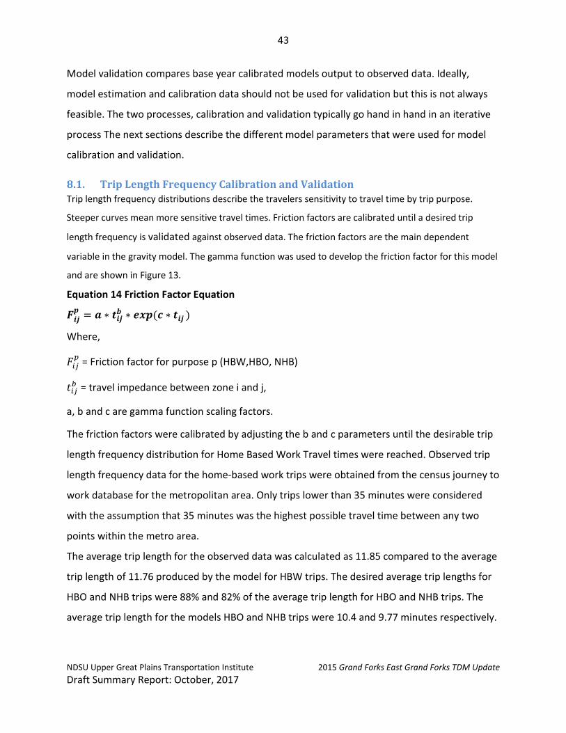
Figure 14 shows the comparison between observed trip length frequencies and the modeled trip length frequencies for HBW trips. The comparison was done for only HBW trips since that’s the only observed data available. The two graphs are very similar to each other.
Coincidence ratios were also calculated to verify the fit between the observed and modeled trip lengths. The coincidence ratio is the area under both curves divided by the the area under at least one of the curves when both curves are plotted together. It measures how the percent of area between that coincides between two curves. Mathematically, the sum of the lower value of the two distributions for each time increment is divided by the sum of the higher value of the two distributions at each increment. Coincidence ratios lie between 0 and 1.0 with a ratio of 1.0 indicating identical distributions. The coincidence ratio calculated between the modeled and observed data was 0.89 showing a strong coincidence between modeled and observed trip lengths.
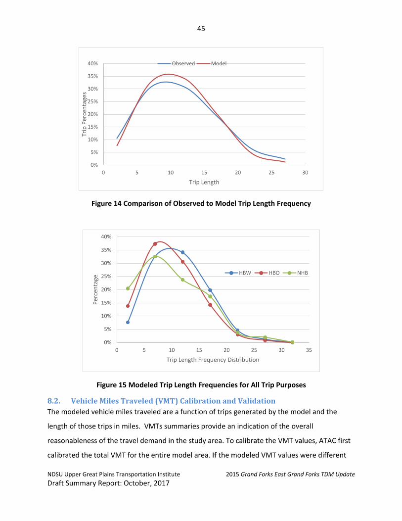
Given Figure 14 and the coincidence ratio calculations, the trip length frequency and average trip lengths were reasonably calibrated and validated. , it is reasonable to assume that trip length frequencies had been reasonably validated with observed data. Figure 15 shows the modeled trip length frequencies for all purposes.
0
100000
200000
300000
400000
500000
600000
700000
800000
900000
1000000
1100000
0 10 20 30 40 50 60 70 80 90 100
Fric
tion
Fact
ors
Trip Length Minutes
NHB HBW HBO
45
NDSU Upper Great Plains Transportation Institute 2015 Grand Forks East Grand Forks TDM Update Draft Summary Report: October, 2017
Figure 14 Comparison of Observed to Model Trip Length Frequency
Figure 15 Modeled Trip Length Frequencies for All Trip Purposes
8.2. Vehicle Miles Traveled (VMT) Calibration and Validation The modeled vehicle miles traveled are a function of trips generated by the model and the
length of those trips in miles. VMTs summaries provide an indication of the overall
reasonableness of the travel demand in the study area. To calibrate the VMT values, ATAC first
calibrated the total VMT for the entire model area. If the modeled VMT values were different
0%
5%
10%
15%
20%
25%
30%
35%
40%
0 5 10 15 20 25 30
Trip
Per
cent
ages
Trip Length
Observed Model
0%
5%
10%
15%
20%
25%
30%
35%
40%
0 5 10 15 20 25 30 35
Perc
enta
ge
Trip Length Frequency Distribution
HBW HBO NHB

46
NDSU Upper Great Plains Transportation Institute 2015 Grand Forks East Grand Forks TDM Update Draft Summary Report: October, 2017
from the values calculated by multiplying the counted ADTs by length (observed VMTs), ATAC
adjusted the trip generation and vehicle occupancy rates until the model and reported VMT
values were similar. Adjusting the trip generation and occupancy rates changes the total
number of trips that are generated within the transportation model. This in turn increases or
decreases the total number of vehicle miles traveled.
Once the total VMT was reasonable, ATAC checked the VMT distribution according to the
functional class. VMT summaries by functional classification provide an indication of how well
the models assignment procedures perform. They will indicate if the model handles free flow
speeds, capacities or whether the trip assignment function has any issues. To calibrate the VMT
by facility type, if functional class VMT distribution was off target, global speeds by facility type
were adjusted.
Table 22 shows the VMT comparison between modeled and observed VMTs and their various distributions as a percentage of total VMT. The model performs very well in replicating the VMTs for Interstates and Major arterials with VMT differences of less than 2% and had similar distributions to the observed VMTs. The VMTs for Local and rural roads of 5% and -6% respectively which is an acceptable deviation. Collectors had a -12% VMT difference which was the most difference between the modeled and observed VMTs. Overall, the model performs within reasonable deviations in replicating VMTS by functional class.
Table 22 Modeled VMTs compared to Observed VMTs
8.3. Screenline Comparisons Screenlines are barriers to travel between two areas in a travel demand model including natural barriers such as rivers, mountains, etc. and man-made barriers such are interstates and major arterials, railroads etc. Five screenlines were used for the model: BNSF railroad, the Red River, 32nd Ave S., Columbia Rd and I-29. Table 23 lists the Screenlines that were used in the GF EGF model.
Observed VMT
Modeled VMT
Difference % DifferenceObserved
DistributionModeled
DistributionInterstate 101,054 103,024 1,970 2% 21% 21%
Major Arterial 207,238 212,044 4,806 2% 43% 44%Minor Arterial 95,705 95,741 36 0% 20% 20%
Collectors 61,287 54,706 (6,581) -12% 13% 11%Local 5,079 5,320 241 5% 1% 1%Rural 11,340 10,726 (614) -6% 2% 2%Total 481,703 481,561 (142) 0% 100% 100%
47
NDSU Upper Great Plains Transportation Institute 2015 Grand Forks East Grand Forks TDM Update Draft Summary Report: October, 2017
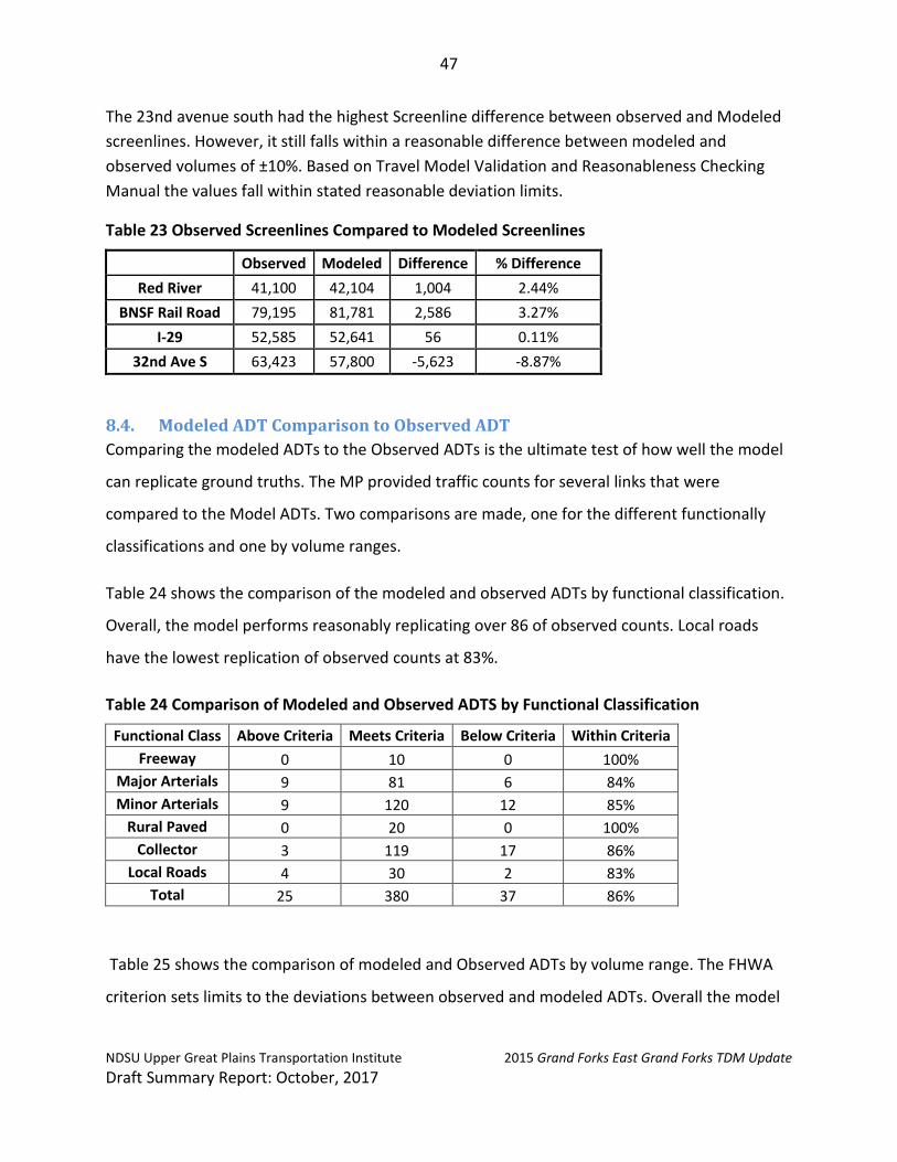
The 23nd avenue south had the highest Screenline difference between observed and Modeled screenlines. However, it still falls within a reasonable difference between modeled and observed volumes of ±10%. Based on Travel Model Validation and Reasonableness Checking Manual the values fall within stated reasonable deviation limits.
Table 23 Observed Screenlines Compared to Modeled Screenlines
Observed Modeled Difference % Difference Red River 41,100 42,104 1,004 2.44%
BNSF Rail Road 79,195 81,781 2,586 3.27% I-29 52,585 52,641 56 0.11%
32nd Ave S 63,423 57,800 -5,623 -8.87%
8.4. Modeled ADT Comparison to Observed ADT Comparing the modeled ADTs to the Observed ADTs is the ultimate test of how well the model
can replicate ground truths. The MP provided traffic counts for several links that were
compared to the Model ADTs. Two comparisons are made, one for the different functionally
classifications and one by volume ranges.
Table 24 shows the comparison of the modeled and observed ADTs by functional classification.
Overall, the model performs reasonably replicating over 86 of observed counts. Local roads
have the lowest replication of observed counts at 83%.
Table 24 Comparison of Modeled and Observed ADTS by Functional Classification
Functional Class Above Criteria Meets Criteria Below Criteria Within Criteria Freeway 0 10 0 100%
Major Arterials 9 81 6 84% Minor Arterials 9 120 12 85%
Rural Paved 0 20 0 100% Collector 3 119 17 86%
Local Roads 4 30 2 83% Total 25 380 37 86%
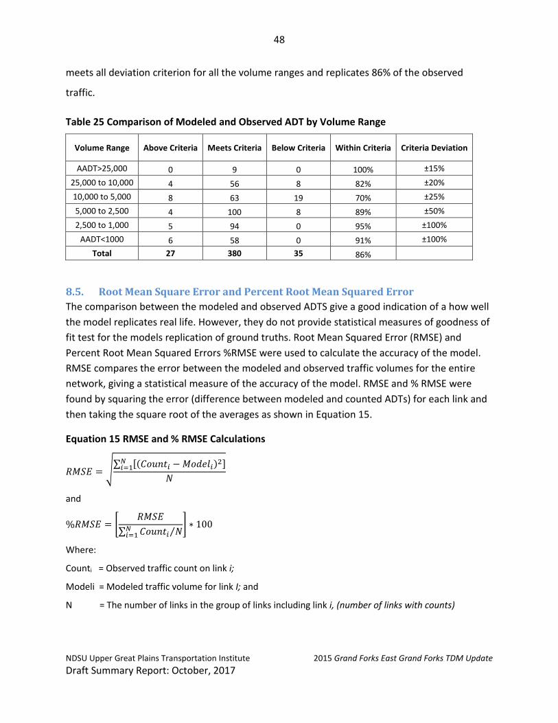
Table 25 shows the comparison of modeled and Observed ADTs by volume range. The FHWA
criterion sets limits to the deviations between observed and modeled ADTs. Overall the model
48
NDSU Upper Great Plains Transportation Institute 2015 Grand Forks East Grand Forks TDM Update Draft Summary Report: October, 2017
meets all deviation criterion for all the volume ranges and replicates 86% of the observed
traffic.
Table 25 Comparison of Modeled and Observed ADT by Volume Range
Volume Range Above Criteria Meets Criteria Below Criteria Within Criteria Criteria Deviation
AADT>25,000 0 9 0 100% ±15% 25,000 to 10,000 4 56 8 82% ±20% 10,000 to 5,000 8 63 19 70% ±25% 5,000 to 2,500 4 100 8 89% ±50% 2,500 to 1,000 5 94 0 95% ±100%
AADT<1000 6 58 0 91% ±100% Total 27 380 35 86%
8.5. Root Mean Square Error and Percent Root Mean Squared Error The comparison between the modeled and observed ADTS give a good indication of a how well the model replicates real life. However, they do not provide statistical measures of goodness of fit test for the models replication of ground truths. Root Mean Squared Error (RMSE) and Percent Root Mean Squared Errors %RMSE were used to calculate the accuracy of the model. RMSE compares the error between the modeled and observed traffic volumes for the entire network, giving a statistical measure of the accuracy of the model. RMSE and % RMSE were found by squaring the error (difference between modeled and counted ADTs) for each link and then taking the square root of the averages as shown in Equation 15.
Equation 15 RMSE and % RMSE Calculations
𝑅𝑅𝑅𝑅𝑆𝑆𝐸𝐸 = �∑ [(𝐶𝐶𝑓𝑓𝐶𝐶𝐶𝐶𝑡𝑡𝑖𝑖 − 𝑅𝑅𝑓𝑓𝑀𝑀𝑒𝑒𝑀𝑀𝑖𝑖)2]𝑁𝑁𝑖𝑖=1
𝑁𝑁
and
%𝑅𝑅𝑅𝑅𝑆𝑆𝐸𝐸 = �𝑅𝑅𝑅𝑅𝑆𝑆𝐸𝐸
∑ 𝐶𝐶𝑓𝑓𝐶𝐶𝐶𝐶𝑡𝑡𝑖𝑖𝑁𝑁𝑖𝑖=1 𝑁𝑁⁄
� ∗ 100
Where:
Counti = Observed traffic count on link i;
Modeli = Modeled traffic volume for link I; and
N = The number of links in the group of links including link i, (number of links with counts)

49
NDSU Upper Great Plains Transportation Institute 2015 Grand Forks East Grand Forks TDM Update Draft Summary Report: October, 2017
Table 26 shows the %RMSE by volume range. The %RMSE is below the typical deviation limits
for all the volume ranges shown indicating a good fit between the modeled and observed traffic
volumes. This is an indication that the model is performing reasonably in replicating observed
traffic.
Table 26 RMSE Comparison by Volume Range
Volume Range RMSE (%) Typical Limits (%)
AADT>25,000 0.0543 15-20 % 25,000 to 10,000 0.1556 25-30 % 10,000 to 5,000 0.2502 35-45 % 5,000 to 2,500 0.342 45-100 % 2,500 to 1,000 0.5291 45-100 %
AADT<1000 0.9871 >100 %
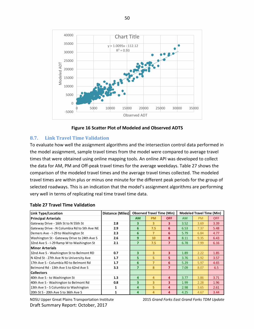
8.6. Scatter Plots, R Squares of Model and Observed Traffic Scatter plots of the modeled traffic volumes against the observed traffic volumes are a good indicator of the model’s fit. Figure 16 shows the scatter plot of modeled traffic volumes versus observed counts. The scatter plot suggests that the amount of error in the modeled volumes is proportional to the observed traffic count which is an indication of a good fit between the model and the observed traffic counts.
The R-square (coefficient of determination) is the proportion of the variance in a dependent variable that is attributable to the variance of the independent variable. They typically measure the strength of the relationships between the assigned volumes and the traffic counts. It measures the amount of variation in traffic counts explained by the model. The modeled R-square of 0.93 shows a strong linear relationship between modeled and observed traffic counts.
50
NDSU Upper Great Plains Transportation Institute 2015 Grand Forks East Grand Forks TDM Update Draft Summary Report: October, 2017
Figure 16 Scatter Plot of Modeled and Observed ADTS
8.7. Link Travel Time Validation To evaluate how well the assignment algorithms and the intersection control data performed in the model assignment, sample travel times from the model were compared to average travel times that were obtained using online mapping tools. An online API was developed to collect the data for AM, PM and Off-peak travel times for the average weekdays. Table 27 shows the comparison of the modeled travel times and the average travel times collected. The modeled travel times are within plus or minus one minute for the different peak periods for the group of selected roadways. This is an indication that the model’s assignment algorithms are performing very well in terms of replicating real time travel time data.
Table 27 Travel Time Validation
y = 1.0095x - 112.12R² = 0.93
-5000
0
5000
10000
15000
20000
25000
30000
35000
40000
0 5000 10000 15000 20000 25000 30000 35000
Mod
eled
ADT
Observed ADT
Chart Title
Link Type/Location Distance (Miles)Principal Arterials AM PM OFF AM PM OFFGateway Drive - 16th St to N 55th St 2.8 3 3 3 3.52 3.69 3.39Gateway Drive - N Columbia Rd to 5th Ave NE 2.9 6 7.5 6 6.53 7.37 5.48Demers Ave - I-29 to Washington St 2.3 6 7 6 5.79 6.84 4.77Washington St - Gateway Drive to 24th Ave S 2.6 9 10 8 8.11 9.35 6.4332nd Ave S - I-29 Ramp W to Washington St 2.1 7 7.5 7 6.78 7.99 6.16Minor Arterials 32nd Ave S - Washington St to Belmont RD 0.7 3 3 3 1.89 2.22 1.85N 42nd St - 27th Ave N to University Ave 1.7 5 5 5 3.76 3.92 3.5717th Ave S - Columbia RD to Belmont Rd 1.7 6 7 6 5.29 5.97 4.65Belmond Rd - 13th Ave S to 62nd Ave S 3.3 7 8 7 7.09 8.07 6.5Collectors40th Ave S - to Washington St 1.3 4 4 4 3.77 3.86 3.7140th Ave S - Washington to Belmont Rd 0.8 3 3 3 1.99 2.28 1.9613th Ave S - S Columbia to Washington 1 4 5 4 2.98 3.65 2.6120th St S - 20th Ave S to 36th Ave S 1 4 4 4 4.25 4.67 3.44
Observed Travel Time (Min) Modeled Travel Time (Min)

51
NDSU Upper Great Plains Transportation Institute 2015 Grand Forks East Grand Forks TDM Update Draft Summary Report: October, 2017
9. CONCLUSIONS This document describes the development, calibration and validation of the GF-EGF MPO base 2015 TDM. Several improvements were made to previous modeling efforts including the addition of Freight movements and better representation of capacities. Overall the model replicates observed travel demand within typically accepted deviation limits.
Related Documents