APL-STAT A Do-It-Yourself Guide to Computational Statistics Using APL James B. Ramsey New York University Gerald L. Musgrave University of Michigan LIFETIME LEARNING PUBLICATIONS Belmont, California A division of Wadsworth, Inc.

Welcome message from author
This document is posted to help you gain knowledge. Please leave a comment to let me know what you think about it! Share it to your friends and learn new things together.
Transcript

APL-STATA Do-It-Yourself Guide
to Computational StatisticsUsing APL
James B. RamseyNew York University
Gerald L. MusgraveUniversity of Michigan
LIFETIME LEARNING PUBLICATIONSBelmont, California
A division of Wadsworth, Inc.

In preparing APL-STAT we were fortunate to have the help of manyfriends and colleagues. Rather than attempt to explain their individualcontributions we simply list their names and express our thanks to each ofthem: Bert Alexander, Alea Curtis, Dorothy Dixson, David Edelman, JohnHause, Robert Hessen, John Kassionas, Jan Kmenta, AlexanderKugushev, Charles Moore, Thomas Gale Moore, Jan Musgrave, RichardW. Parks, Virginia Perry, Alvin Rabushka, Grace Ramsey, ShannonRamsey, Robert Rasche, Bernard Scheier, Bert Schoner, Andy Silver,
, Barbara Snarr, and Mike Sullivan.
© 1981 by Wadsworth, Inc. All rights reserved. No part of this book maybe reproduced, stored in a retrieval system, or transcribed, in any form orby any means, electronic, mechanical, photocopying, recording, orotherwise, without the prior written permission of the publisher, LifetimeLearning Publications, Belmont, California 94002, a division ofWadsworth, Inc.
Printed in the United States of America
1 2 3 4 5 6 7 8 9 10--85 84 83 82 81
Library of Congress Cataloging in Publication Data
Ramsey, James Bernard.APL-STAT, a do-it-yourself guide to computational
statistics using APL.
Includes index.1. Statistics-Data processing. 2. Econometrics
3. Mathematical statistics-Data processing. 4. APL(Computer program language) I. Musgrave, Gerald L.,joint author.II. Title.QA276.4.R35 519.5'028'5 80-15016ISBN 0-534-97985-8
Contents
Preface ix
Notes to Instructors xiii
11.11.2
IntroductionOverview of APL 1Road Map of Where We Are Going and How We Will GetThere 3
1
2 Getting Started2.1 Some Keying Conventions 62.2 Simple Arithmetic 62.3 Arrays 10Summary 12Exercises 12
6
33.13.23.33.43.53.6
3.7
Some Elementary StatisticsThe Computer Reads from the Right 15Two Arguments or One? 16Variables and Assignment 17A System Command: )VARS 18How to Calculate a Mean 19Two Other Measures of Central Tendency: The Geometricand Harmonic Means 21Sample Variance and Standard Deviation 23
15
iii

77.17.27.3
88.18.28.3
iv Contents
3.8 Correcting Typing Errors 253.9 Mean and Variance of Sample Probabilities 26Summary 28Exercises 29
4 How to Write Your Own Function4. 1 The Sample Median 344.2 Function Definition 41Summary 49Exercises 51
5 Some More Statistics5.1 Some Basic Statistics 585.2 Dummy, Local, and Global Variables 63Summary 66Exercises 67
6 Higher and Cross Product Moments and Distributions6.1 Some Useful Distributions (Binomial, Poisson) 736.2 Histograms 766.3 The Normal Distribution 83Summary 87Exercises 89
Data and Information-How to Get It In and OutNumeric and Character Arrays 97Entering Data Inside a Function 101Saving Your Workspace When Using theComputer Terminal J06
Summary 111Exercises 112
More on FunctionsFunction Display, Correction, and Editing 116Diagnostic Procedures 121A Case Study in Program Development and the Location andCorrection of Program Errors 127
Summary 137Exercises 138
34
57
72
97
116
99.1
Elementary Linear Regression, Goodness of Fit, and Analysis
of Variance (ANOVA) ProblemsIntroduction to Linear Regression 144
144

1212.112.212.312.4
Contents
9.2 An APL Program for Linear Regression Analysis 1459.3 Goodness of Fit, Contingency Tables, and ANOVA
Problems 1489.4 Calculating the Chi-Square and F Distributions 159Summary 165Exercises 166
10 Matrix Algebra in APL-How Simple It Is10.1 Vectors, Matrices, and Arrays 17210.2 Elementary Matrix Operations 17410.3 Transpose of a Matrix 17810.4 A Not So Elementary Operation: Matrix Inverse 179Summary 185Exercises 186
11 Higher-Order Arrays11. 1 Reduction Function 19111.2 Compression 19711.3 Expand Function 19911.4 Reverse or Rotate Function 20011.5 Transpose Function 20511.6 Ravel, Catenate, Laminate 20911.7 Take and Drop Functions 213Summary 215Exercises 217
Inner and Outer Products-Matrix ManipulationInner Product: Some New Ideas 221Outer Product 223An Economic Example (Production Functions) 225Two More Not-So-Elementary Matrix Operations(Kronecker Product, Determinant) 229
Summary 235Exercises 236
13 Linear Regression13.1 Covariance and Correlation Matrices 24013.2 Some Initial Linear Regression Statistics 24313.3 SiInple and Partial Correlation Coefficients 24513.4 Creation of a Regression Routine 24613.5 Bells and Whistles Section 258SUlnmary 262Exercises 262
v
172
191
221
240

1414.114.214.314.414.5
vi Contents
Other Simple Regression Equation EstimatorsSimultaneous Equation Models 268Two-Stage Least Squares 269Instrumental Variables 272Aitken's Generalized Least Squares 275Durbin's Estimator in First Order Auto-regressiveModels 278
14.6 k-Class Estimators in Simultaneous Equation Systems (OLS,2 SLS, and Limited Information Maximum Likelihood) 282
Summary 288Exercises 289
268
Appendix AA.IA.2A.3
The Computer: Where It Is and How to Get Access to ItAccount Number and Password 294Log-On Procedure 295Log-Off Procedure 297
294
Appendix B Longley BenchmarkAppendix C APL Character SetAppendix D Saving Your Workspace on The IBM 5110 MicrocomputerAppendix E Data Set 'Macro'Function GlossaryBibliographyAnswers to The ExercisesIndex
302304307310316330332338
Preface
Please Read This Before Reading the Text!
This book explains how to perform both simple and complex statisticalcalculations using APL. "APL" is an acronym for "A ProgrammingLanguage"-a computer programming language that is ideal for the computational work done in statistics.
The authors are both economists, and the content reflects their professional interests. However, political scientists, physicists, sociologists, industrial psychologists, public health and dental researchers, and othershave used this book and found it helpful.
No previous knowledge of computers, computer programming, or methods involved in statistical computation will be needed to understand thisbook. You will start from the most elementary statistics and progress tomore complicated procedures on a gradual step-by-step basis. The numerous examples, exercises, and statistical applications are drawn from avariety of fields. Emphasis is placed on how to obtain the statistical resultswith ease. Using this book you will be able to perform computations thatotherwise would be so cumbersome or time-consuming that you would notdo them. You also will be able to perform experiments and computersimulations with relatively little effort.
The APL statistical procedures presented are useful to researchers,analysts, managers, and anyone concerned with statistical calculations. Webelieve that when you have seen how easy it is to perform these computations, you will be as pleasantly surprised as we were. If you are familiarwith computers here is a dramatic example of the simplicity of APL compared to the FORTRAN statements used to compute the arithmetic mean.If you are a novice in these things don't be frightened--everything will beexplained.
vii

viii Preface
APLX+{J
O+-AVE+( +/X)+pX
10
20
F0RTRANDIMENSI0N X (1000)READ (5,99)N
99 F0RMAT (14)READ (5,100) (X(I), 1== 1,N)
100 F0RMAT (9F8.0)SUM == 0.0D0 10 J == I,NSUM == SUM + X(J)AVE = SUM/NWRITE (6,20)AVEF,0RMAT (FI0.4)END
To estimate the parameters of Y = B 1 + B2 X 2 + Ba Xa + . · ·via multiple regression, you could type in APL:
An Exampleof F(/)RTRANand APL
Use of [1
in MultipleRegression
B +- Y!BX
In other computer languages an equivalent program might take 50 statements.
This book is not just an introduction to APL programming, althoughmany people have learned APL from it. Certainly it is not a statisticstextbook, but readers have commented that they never really understoodcertain statistical concepts until they "tried real numbers to see how theformulas worked." This book is a valuable aid to understanding statisticsbecause it actually computes results and even displays probability distributions graphically. By the time you finish you will know a lot about APLprogramming. And after you spend a few hours at the computer, you willfind that it is easier to program your own work than it is to learn to use the"canned" (F,0RTRAN) routines available at the computer facility. Moreimportantly, you will understand what you are doing and how the resultsare obtained. We have long maintained that the less you are asked toaccept unquestioningly, the better is your intellectual health and thegreater will be your interest in statistical subjects.
This book is not primarily a textbook. It is a book for the person whounderstands basic statistics, who wants a painless way to compute results,and yet wants to know what is really going on. We think that teachers ofbasic or applied statistics and especially econometrics will find our approach using APL to be an important part of a practical statistics course.Students are often assigned "artificial," "theoretical," or "academic"problems, situations, and exercises. These assignments are not made because the instructor thinks such things are important. Actually, most instructors understand the difficulty of tackling real statistics problems. Consequently, when the amount of computational pain the student (andteacher) must go through to get the statistical result is compared to the"statistics" that can be taught, a stress on pure theory almost alwaysresults. Thus, after a course (or even several courses), an individual maybe unprepared to solve the first problem-how to perform the calculations!The use of APL minimizes these difficulties.

Preface ix
Purpose ofTheseComments
We think that when you complete APL-STAT you will agreeprogramming can be easy !
Because the text proceeds in a carefully structured sequence it is important that you follow it exactly and that you make sure you thoroughlyunderstand each section before moving to the next. Later sections assumethat prior sections have been mastered. You should do the exercises andcheck your answers in the back of the book. Above all, you can teachyourself a lot by experimenting, so try it.
If you forget something, the primitive function glossary at the back ofthe book will help you recall earlier materiaL If you need more information, the side of most _pages has brief comments. These comments containthe name and symbol of the APL operator introduced on that page. Youwill be able to flip through the book quickly and locate what you want,using the comments. They also provide a quick visual guide to the majortopics in any section.
We have a request. In the back of the book is an error sheet for recordingour omissions, bad language (though never foul!), and other sins. We wouldbe most obliged if you would send us this error sheet with your comments.The next edition will then be much better with your help.
JAMES B. RAMSEY GERALD L. MUSGRAVE

x
Note to Instructors
Instructors can assign much more meaningful examples and exercisesusing the procedures in this book than using either canned programs orhand calculation. Students will not be spending time in tedious calculationor in using the computer as a black box. Students will be able to performcalculations, including complex matrix algebra, know how they are done,and see the numerical results. They will be able to obtain results theyunderstand. One example is where a multiple regression model requiresthe intercept to be "forced" through zero. It is surprising how simple themathematics of this is (not having a column of ones in the regressor Xmatrix). It is also surprising how few preprogrammed packages allow thisoption. In APL you can modify your program to handle this change in amatter of moments.
Computer simulation and generation of distributions become a relativelytrivial task in the hands of an APL-proficient student. We could enumeratea long list of such examples, and once you start you will see them too.Also, we have included our benchmark program data on the Longley regression problem in Appendix B. You may find it interesting to comparethe computational accuracy of APL programs with the canned ones onyour home computer or at your computer center.
In using this book as a text you might consider the following ideas. Thetitles of certain sections, e.g., The Normal Distribution in Chapter 6, arestarred. These starred sections involve mathematical material which maybe beyond the scope of an elementary course in statistics that doesn't havea mathematical prerequisite. Any APL instructions introduced in suchsections will not be used anywhere else in the text without reexplanation.So starred sections can be dropped without fear of losing some importantinformation about APL.
The book is carefully structured in that it follows the usual pattern oftopics in the introductory statistics course and only uses as much APL asis needed to get the job done. Consequently, it is important that, except forthe starred sections, the sequence be followed and sections are not skipped.
If you decide to alter the presentation of statistical subjects, have your

Note to Instructors xi
students read the APL-material in sequence, even if they skip the earlierpresentations of the statistics. A number of readers have used this approach and found it to be satisfactory. In these cases the readers eitherknew statistics or were not interested in statistics per see They wanted tolearn APL and found this approach to be effective. One reason for this isthat APL instructions are introduced to solve specific problems rather thanpresented in the abstract.
Each chapter has a large number of exercises and applications. Theexercises help in exploring the use of APL concepts, functions, and symbols. The statistical applications help extend the depth and breadth of APLuse. Throughout the book, experimentation is encouraged to expand andintensify interest and understanding.
An elementary nonmathematical course in statistics would usually stopat Chapter 9, which covers contingency tables, analysis of variance, andsimple linear regression with one regressor. Chapters 10, 11, and 12 introduce various aspects of matrices and prepare the way for multiple linearregression analysis and topics that might be regarded as more "econometric." You may find that the use of APL will allow you to cover Chapters 10through 13 as well. This is important since the rudiments of matrix algebracan be taught quickly using APL. The benefit will be that you can enableyour students to master multiple linear regression and more complicatedanalysis of variance techniques more easily.
Three administrative matters might be of interest. Many computer centers have only a few APL terminals. Don't let this apparent difficulty slowyou down. First, if the terminals use a typing ball or a daisy wheel, thecenter can obtain APL balls or print wheels. They are easy to switch, arelow in cost, and small adhesive labels are available for the keys. Second, ifthe terminals use a non-APL matrix printer or if the terminals are CRT'swithout APL characters, another solution is available. A Mnemoniccharacter set that substitutes for the APL symbols is available. The multiple regression example in the preface was coded as
y+-YffiX
using the standard APL character set. In the Mnemonic character set itwould be written as
Y+Y.DQX
Appendix C contains both the standard and Mnemonic character sets.Third, some computers have implemented only the monadic version ofdomino. In this case you simply enter the following two lines
VYDQX(~((~X)+.xX»)+.X((~X)T.XY)V
when you enter YDQX the result is the same as if YffiX 'had been entered.If in using the book you have any comments that would be helpful to
others please pass them along to us and we will incorporate them in thenext edition.


1
Introduction
1.1 Overview of APL
APL is a powerful and versatile computer programming language. Whenyou use this language to communicate with the computer it will be as ifyollwere personally operating the machine. APL is designed to operate onsmall microcomputers no larger than a typewriter, on minicomputers thesize of one or two office desks, and on large maxicomputers the size of atruck. No matter how large or small the computer, once you log-on to thesystem it will appear from your perspective that you have a one-to-onerelation with the computer. The APL contained in this book has been usedon micro-, mini-, and maxicomputers produced by a variety of manufacturers. We found the APL language to be remarkably similar in all of thesecases.
Administrative Procedures
The procedures used to log-on to the various systems that we have usedvary greatly. Each computer center has its own administrative procedures,keywords, passwords, and account verification methods. In addition, youusually need to connect your computer terminal to the computer itself andthis process can be mysterious at first. There is really nothing to this at all.Nevertheless, sometimes people who hang around computer centers makea big deal about the administrative and technical matters surrounding theuse of the machine. The truth of the matter is that the procedure is muchthe same as getting a key for an office, registering for a class, or signing upfor Little League. It's a hassle. Every organization thinks that there is onlyone way to do it, and yet every way is different. Appendix A contains abrief description of how it is done at the Stanford and NYU computercenters, and on an IBM 5120 desk-top computer. This description should
1

2
CLEAR WS
)OFF
State Diagram
Introduction
allow you to understand better the procedures that are used with yourcomputer. In a short time the mystifying intricacies of gaining access to thecomputer become second nature. You type a few words and numbers andyou are ready to go.
The APL Keyboard
We have included a few diagrams of typical APL keyboards in AppendixA. The alphabetic characters are in exactly the same position as they areon a standard typewriter. These letters are all capitals but (wouldn't youknow it) they are in the lowercase positions. Holding the shift key downwhile pressing a specific key enters a special APL symbol. Each of thesesymbols performs a specific operation in APL. As you can see, thekeyboards are almost identical, and in the very few instances where someminor differences do exist we will explain them. One of the most frightening things that the new APL programmer encounters is the APL characterset. All those strange symbols are indeed foreboding. However, our experience has been that the symbols are easy to learn. They are not muchmore difficult to learn than the international road signs, especially if youtake them one at a time in the context of an actual problem.
Some General Features of APL
Now suppose that you are sitting in front of the keyboard and you havelogged-on. The computer has responded with the message CLEAR ws. Thecomputer is indicating that you have been allocated a part of thecomputer-APL calls it a Work Space-named CLEAR. Now you cancommunicate with the computer, and it is in fact much like an electronichand-held calculator except that it is much more powerful. To tum off thecomputer you simply type )OFF, for example, and log-off. You will soonsee how APL can be used as a very powetful calculator in the immediateexecution mode. However, it can do much more.
You can define a set of instructions that will perform tasks such asbalancing a checkbook; computing means, standard deviations, and regression coefficients; or directing the computer to simulate a Las Vegascasino game. In APL, the set of instructions is called a defined function.After the function has been defined you simply refer to it by name. Thesame instructions, operating on different data, can be used over and overagain.
Figure 1.1 is a state diagram that represents these three APL modes.When you log-on you are given a clear work space, you are in immediateexecution mode, and you have a powerful calculator at your disposal. Youcan enter data, process the data with a one-line APL expression, define anentire new work space with different functions and data, and test yourfunctions on a line-by-line basis before you program the whole set ofinstructions.

1.2 Road Map of Where We Are Going and How We Will Get There 3
Figure 1.1
Enter &execute APLstatements
To define a function enterdNAME of function
-.DTo close a functionenter 11
Enter data (
Edit functionin developmentstage
Then you can define your own function, edit any part of it, or modify itfor a particular application. Also, should a function stop because of aprogramming error and further processing thereby be suspended, you cancorrect the error by editing the function and then resume the function'sexecution from the point of suspension. You need not start from the beginning if your previous calculations were correct.
A function is executed by simply entering its name. You can specify theparticular data set to be processed, and your function can call other functions, request data, and produce results for use by other functions. Inaddition, you can trace the execution of your function by having the resultsof any line or group of lines displayed-all of this without having to writeany output statements. When your function's execution is completed itreturns you to immediate execution mode where you began. We hope thatthis sounds simple, straightforward, and like something you can dobecause it is!
1.2 Road Map of Where We Are Going and How We Will Get There
In the next chapter you will learn how to use APL as a calculator. Afterthese basics are under your belt, the general presentation is to explain astatistical problem and then to solve it using APL. On the way to thesolution the various APL functions and programming methods are presented and explained. We first discuss the sample mean and median, stan-

These matrixmethods are usedin the solutionsof more complexstatisticalproblems
Statistics
Chapters3, S, 6,'9,12, 13, 14
MaitixMethods
ct'-Hi~Order'. ~ys
ci\aPten 10.. 1t
Functions oftenuse these methods
Many of our statisticalprocedures are writtenas defined functions
1These primitivefunctions are combinedmto routmes
F,unctionDeJinitioo
Chapters4,05, <i, 7, 8
tAlter the resultsI of Computations
'. ,
Chapters 2, 3
Systems .cio~
" "'~.',
SylllC!D1I Y~bIes
Chapter lS
+, -, x, +, I. p, etc.
After defining a 1function it can beused as any otherprimitive function
Systems commands can beused to organize dataand work space
Processing ofscalars & vectors Basic Deft",tions & Syntax
-....:..---:----:---------1.~ Execution of FUDCtion
Executing functionsto organize data..
Functions are oftenused to organizeand manipulate data
Chapters7, 11, 14
D$ta Entry andMani~ulation
'Figure 1.2
1.2 Road Map of Where We Are Going and How We Will Get There 5
dard deviation, covariance, and higher order moments. Then we investigate a number of the most prominent statistical distributions, including thebinomial, Poisson, and normal density and cumulative distribution functions. After you learn how to handle more complex data structures in APLand to write more general and powerful functions you will learn how todiagnose and correct programming errors. After you go through a casestudy using APL in a research project, we present an introduction toelementary linear correlation and regression, analysis of variance, and thechi-square and F distributions. Next we show how to do matrix algebra inAPL, including the operation of matrix inversion, which is performed withone symbol, IT]. Multidimensional arrays are discussed in Chapter 12,where the various APL functions are explained in relation to these higherorder arrays. The final chapters concentrate 00 computational statisticsrelated to multiple linear regression, two-stage least squares, instrumentalvariables, Aitken estimators, Durbin's First Order Autoregressive Models,and K -class estimators including limited information maximum likelihoodestimators.
Don't let this impressive soundingjargoo put you off. The first half of thebook has been understood by good high-school students, and they wereable to write APL programs after only a few hours of study. The laterchapters have been used in both undergraduate and graduate classes. Also,the statistical routines have been used by a number of our colleagues intheir statistical research. So you can see that while much of the material istechnical, it progresses at a measured rate. Figure 1.2 is a schematic representation of APL-STAT. It might help you to visualize how the variouscomponents of APL are related.
We can summarize our position this way:
APLTRY IT-YOU'LL LIKE IT
So turn the page and let's go ...

2
Getting Started
2.1 Some Keying Conventions
Now that you are seated comfortably in front of your terminal or minicomputer, everything is switched on, and the terminal is set to receive yourinstructions in APL, we can begin. Our first task is for you to gain somefamiliarity with the use of your keyboard as shown in figure 2.1.
Sometimes we want to indicate to you very clearly that there is a blankspace. For example, consider the character string ABCD EFG, which youtype by hitting the A, B, C, D keys, the space bar, and then the keys E, F,and G. Blank spaces will be indicated, but only when we need to stress thatthere is a blank, by printing an ampersand (&) in a subscript position. Inthe above example, we would print ABCD&EFG. You can read this as: A,B, C, D, and E, F, G. You will not find the & character on your APLkeyboard; we use it in the earlier chapters to emphasize blanks until youreye is accustomed to the idea.
2.2 Simple Arithmetic
ArithmeticFunctions+,-,X,7-
6
We will start by making sure we know how to add (+), subtract (-),multiply (x), and divide (-7-) numbers on the computer. The symbols +, -, x,
and -;- are the symbols for the mathematical operations of adding, subtracting, multiplying, and dividing, respectively. On the IBM 5120, for example, they are found on the far right-hand side of the keyboard, next to thekeys with the integers from 0 to 9. You may also use the numbers shown onthe top row of the main keyboard and the arithmetic functions shown at theend of that row (this is the most common configuration).
You instruct the computer to perform a calculation by hitting the RETURN or EXECUTE key; the instruction is executed only after you hitthe key.

Figure 2.1 IBM 5120desktop computershowing the APLcharacter set, numericpad, and specialfunction keys.
IBM 5120 showingkeyboard charactersthat can be enteredusing the command key.
Add +
2.2 Simple Arithmetic
This photograph showing a 5120 desktop computer can be programmedin either Basic or APL with the flip of a switch. The keyboard is exactlylike a standard typewriter in that pressing the shift key (either of the keyswith the wide arrows on the bottom rank of keys) results in the APL characters being entered into the computer. A convenient feature is that byholding the command key (CMD, on the far left) and pressing one of thekeys on the top row will produce an entire command. For example, holdingdown CMD and pressing I results in the command )LOAD being enteredautomatically.
This photograph shows the special overstruck characters that can beproduced with one stroke. The command key is held down and any of theindividual keys now represents a new symbol or combination of key strokes.For example, pressing the CMD key and the F key results in the divide quador domino function being entered. If the machine were in the Basicprogramming mode the characters INPUT would have been entered. Usingthe CMD key saves a number of key strokes and is a handy feature.
Addition
1-t2
3
7
If you did not get the answer after keying in the digit 2, hit the RETURNor EXECUTE key. Now try addition with decimals:
1.2+0.6
1.8

8
SYNTAX ERROR
Minus
Negative Numbers
Getting Started
But if you key in
1 8
This does not look right! What happened?Clearly, embedded blanks in real numbers (numbers that include a dec
imal) cause problems! So do not embed blanks in real numbers. You willunderstand why you got 1 & 8 and not 1.8 by the end of this chapter.
Try
1+
SYNTAX ERROR
1+
You have made an error and the symbol /\ (a caret) marks the point atwhich the error occurred. Unfortunately, we all get much too familiar withthis symbol! The error was called a syntax error because the statement"execute 1 +" is ungrammatical; it does not make sense to tell the computer to "add 1." The computer's response is to say, "Add 1 to what?" or"How can I do this?"
Subtraction
Key in 3, minus sign (-, which is next to the plus (+) sign), and 2, thenEXECUTE:
3-2
1
or
2-3
1
Notice that on the last response negative 1 was printed by the computer as-1. The superscript negative indicates the negative sign of the number andmust be carefully distinguished from the - in - 1. In the latter casethe symbol - represents the operation of subtraction. How do we know thedifference? By position. For example,
-2 represents the number "negative 2";- 2 represents the operation of subtracting 2 from whatever is to the left
of -.How do you type the nUlnber "negative 2"? This is done by typing the
symbol -, which is upper-shift 2 on the keyboard. Try it.
2
2
(Remember to hit EXECUTE!)

2.2 Simple Arithmetic
Now use the minus operator symbol key:
-2
9
Multiply x
Divide -.
DOMAIN ERROR
2
What happened here? 3+ gave a syntax error, why didn't -2? The answer is that APL interprets the operation - 2, when nothing is on the left, asthe instruction "Make the argument (i.e., whatever is on the right) thenegative of whatever it is." Try - -2 and - -2. You get 2 in both cases. Trythe following as well:
+2
- +2
2-
So if the + or - functions are on the left of a number, the sign of thenumber is unchanged by + and reversed by - . But if the number is on theleft of thefunction, you will get a syntax error.
Multiplication
6
3.Sx2
7
Division
Try
6-;-3
2
5-;-2
2.5
0-;-4
o
DOMAIN ERROR
10
2.3 Arrays
Arrays
Blanks
Getting Started
We have hit another error. A useful mathematical convention is that division by zero is an undefined operation, and that is what the computer istelling you. In this case the syntax or "grammar" ofthe use ofthe function... is correct, but the operation cannot be performed with the number 0; 0lies outside the domain of validity for the operation of division. But whatabout o... o? Try it.
0 ... 0
1
Without going into details at this stage, merely note that this is anotheruseful convention-in short, an agreement as to what to do with such anoperation.
We will now introduce you to the single most important aspect of the APLlanguage, the array. An array is an ordered arrangement of numbers orcharacters. A simple example is a linear arrangement of numbers, such as1 3 2 4 5, or characters, such as AN&ARRAY. In one form or another,arrays playa vital role throughout this book. Try the following:
3+263
266
and
596
What has happened here? In the second example 2 6 3 is treated as a listor array ofthree numbers, viz., 2, 6, 3 in that order. So an array ofnumbers is created by separating each number in the array by a blank. Anotherway to do it is to key in 2,6,3 where the comma, instead of blanks, separates the individual digits. If you recall the comment made above aboutblanks inside real numbers, you will see that it is dangerous not only foryou to embed blanks in real numbers in an array, but also for you to embedblanks within integers as well.
Try the following:
3+1.2&2.3&3.3&4.1
4.2 5.3 6.3 7.1
3+1.&2&2.3&3&.3
4 5 5.3 6 3.3
If these results seem strange (or if you do not get either result) carefullycheck your keying of numbers and blanks. In the second example, theresult shown occurs because 3 is added to 1., 2, 2.3, 3, and 0.3 in tum;

2.3 Arrays 11
the blanks denote from the right where one number ends and the nextbegins. Also try
3+1.2,2.3,3.3,4.1
4.2 5.3 6.3 7.1
APL and Arrays or
3+ 1 . , 2 , 2 . 3 , 3 , . 3
4 5 5.3 6 3.3
456
Notice here that just as you can add a number to a list of numbers youcan also add a list of numbers to a single number.
3+1&&2&&&364
4 5 367
So much for the blanks. Now let us get back to the main issue: Whatis meant by adding 3 to an array of numbers? Quite simply, and as youwould expect, 3 is added in tum to each of the numbers in the array. Nowtry
APLFunctionsand Arrays
3&2&1-2
1 0 1
The general rule we see is that for any functionf such as +, -, x, or f, anumber n, and an array at, a2, . .. ,ap , the statement "nf array" producesan array nfat, nfa2' ,nfa p , and the statement "arrayfn" produces anarray attn, a2!n, , apfn.
If one array lets you do a series of operations all at once, what willhappen if you use two arrays? Try
1&2&3+1&2&3
246
Clearly, each element of the first array is added to the corresponding element of the second array. Similar results hold for the other arithmeticoperations.

12
LENGTH ERROR
Summary
Getting Started
But what if the two arrays have different numbers of elements in them(i.e., what if the arrays have different lengths)? There will be some elements in one array to which there are no corresponding elements in theother. So if we try to operate on arrays of different lengths, we get aLENGTH ERROR. Try
1&2+1&2 &3
LENGTH ERROR
12+ 1 2 3
II
But the following is fine:
243
+ , -, x, and .;. are arithmetic functions."3+2" adds the numbers 3 and 2; "3-2" subtracts 2 from 3; "3';'2"
divides 3 by 2 : "3 x 2 ., multiplies 3 times 2."+ number" returns the number." - number" changes the sign of the number.
An array of numbers is formed by entering numbers in a list separated byblanks or by commas. We represent blanks where necessary in this text by&. More complex arrays will be discussed later.
Numbers, arrays, and the arithmetic operations that we discussed in thischapter can be combined as follows:
Exercises
Numberf NumberfNumberNumberfNumberf ArrayArray f NumberArray f Array
f ArrayArrayf
yields a number.yields a number.yields Syntax Error.yields an array.yields an array.yields an array only if the arrays have thesame number of elements (the "samelength"). It yields Length Error when thearrays have different lengths.yields an array.yields Syntax Error.
APL PracticeLet's explore the use of the functions defined in this chapter:1. (a) +2 positive two
(b) 2+ Syntax Error

Exercises 13
(c) 1-;-2 one divided by two
(d) - 2 minus two(e) -2 negative two
(f) - -2 minus negative two
(g) - 2 the negative of minus two
(h) -;- 0 Domain Error
(i) 3 -;- 0 Domain Error
(j) 3-;- ( 2- 2) Domain Error
(k) 3+ - 2 three plus negative two
(1) 3-+2 subtract positive two from three
(m) 3 x - 2 multiply three by negative two
(n) 3 x -;- - 2 three times the reciprocal of negative two
(0) 3 x - -;- 2 three times the negative reciprocal of two
(p) - 3x-;- -2 the negative of the answer to (n)
(q) - 3 -;- - 2 the negative of three divided by negative two
2. You can get a better idea about the use of arrays by trying the following exercises:
(a) 1&2&3+2 add a number to an array
(b) 1&-2&3-2 subtract a number from an array
(c) 1& -2&3+ -1&2&-3 add two arrays
(d) (1&-2&3)-(-1&2&-3) subtract two arrays
(e) 1&-2&3- -1&2&-3 subtract two arrays
(f) 1& - 2 &3 x -1 & 2 & - 3 multiply two arrays element by element(g) 1, -2, 3x -1,2,3 same as (f)
(h) (1& -2&3)-;-(-1&4&-3) divide one array by another, element byelement
(i) 1 -23-;--14 -3 same as (h)
(j) 1&2&3 X -1&2 Length Error
(k) 1& 0 &3 X -;-1&O &3 Do you get Domain Error? Why or whynot?
(1) 1- &-2 &3+ 2 add the number two to the array - 2 3 andsubtract the sums from one
Statistical Applications
1. What is the arithmetic average of 10 and 20?
2. What is the reciprocal of the arithmetic mean of the reciprocals of 10and 20? Verify that this number is smaller than the arithmetic averageof 10 and 20.
3. Find the volume of a cube whose sides are 4.5 ft long.

14 Getting Started
4. The following three measurements were taken on one side of a cube:0.00000060,0.00000065,0.00000063. What is your estimate of the volume of the cube?
5. Seven prices for a popular 35 mm SLR camera were collected from arecent photography magazine: $259.95, $245.00, $254.99, $259.99,$259.95, and $249.95.a. Compute an average price for the camera.
b. What is the range of prices?
c. How much more is the highest price than the average price?
d. What would be the percent saved by purchasing at the lowest pricecompared to the highest price?
6. A local business selected a representative week's returned checksdue to insufficient funds or fraudulent accounts. The checks werewritten for $23.41, $184.24, $73.12, $2.48, $32.00, $14.28, $58.61,$84.00, $41.41, $83.27, and $102.87. What would you forecast theyearly total amount of returned checks to be?

3
Some ElementaryStatistics
If you have read the first few chapters in any book on statistics or econometrics, you will have noted that the sample mean appears quite prominently. In fact, if you continue using statistics you will be computing alarge number of means. It will save a lot of time if we can discover a quickway to get the computer to do it. Before tackling our first statistic, we haveto learn an important fact about how a computer reads instructions in APL.
3.1 The Computer Reads from the Right
In order to compute a mean, we need an array of numbers and a knowledgeof how many elements (numbers) it contains. Suppose we have the array(1 2 3 4), which obviously has four elements in it, and we want to calculateits mean. Mathematically, the operation can be written as:
(1 + 2 + 3 + 4)/4 == 2.5
In APL we can enter the following statement:
(1+2+3+4)-i-4
2.5
Great so far. But suppose we entered:
1+2+3+4-i-4
7
Computer ReadsFrom Right to Left
We made another mistake! But this one is a very, very important one toremember. In APL a string of mathematical operations is carried outfromright to left. Since we are accustomed to reading from left to right, youcan see that until you are used to the idea, you can make some bad
15

16 Some Elementary Statistics
mistakes. Indeed, for the next few chapters you are strongly advised topractice reading all the computer statements from right to left.
Consider the first example: (1 + 2 + 3 + 4) -;- 4. The computer doesthe following. Starting from the right, the computer recognizes a number,then a function requiring two arguments, such as -i-, x, -, or +, then a rightparenthesis. This parenthesis tells the computer to keep going to the leftuntil it encounters a matching left parenthesis; then whatever is containedbetween the left and right parentheses is to be divided by four. Within theparentheses the computer recognizes a 4, the function, +, and then thenumber 3. It perlorms the operation 3 + 4 and stores the result. Proceeding to the left, it recognizes another function symbol, +, followed byanother number, 2, so it adds 2 to (3 + 4), and so on.
All of this is simple enough, so let us try a trickier example. Do this oneby ha.1d first and then check your result on the computer.
1+2-3-4+5-6-7
10
If you got -12 instead of 10, then that is exactly what we wish to explain. Ifwe add parentheses, the above expression can be written as
1+(2-(3-(4+(5-(6-7)))))
10
In case you haven't got it yet, the following table should help:
OperationNumber Operation Result
6-7 - 11
2 5- -1 6
3 4+6 104 3-10 7
2- - 7 956 1+9 10
3.2 Two Arguments or One?
Monadic FunctionsDyadic Functions
A few paragraphs back we said that the functions -i-, x, -, and + require twoarguments, but in Chapter 2 we successfully used the + and - functionswith only one argument, provided that the argument was on the right of thefunction, not the left. At the moment all of this may be confusing, but itwon't be after we show you how useful it is to have a function that can takeeither one or two arguments.
First, a little terminology in case you dip into an APL manual or talk to aprogrammer friend: functions that take two arguments are said to bedyadic, and those that have one argument are monadic; 1+2 is a dyadic useof +, +2 is monadic. The symbols for most functions are used to represent

3.3 Variables and Assignment 17
Dyadic function:
Reciprocal
SYNTAX ERROR
both an operator that is dyadic and one that is monadic-two functions forthe price of one symbol!
For example, the function.;. can be used in two ways:
Monadic function: Symbol: .;-, function: reciprocalExample: .;.2
.5
Symbol: .;., function: divisionExample: 4.;.2
2
In the first case the symbol.;. indicates the reciprocal (or 1 -;- argument); inthe second case the symbol -;- indicates the operation of division (argument2 divided by argumentl ).
The symbol - represents two functions-the monadic function of arithmetic negation (more simply, "changes the sign") and the dyadic functionof subtraction. The symbol + represents addition in its dyadic form; in itsmonadic form it preserves the identity of the argument, i.e., + numberreturns the number itself. The symbol x is used for both the dyadic function of multiplication and for the monadic function "signum," which willbe mentioned later.
Recall that with monadic uses the function comes first, then the argument. A number followed by a function and nothing else gives aSYNTAX ERROR.
In using symbols that can represent different functions depending onwhether they are being used monadically or dyadically, remember to readfrom the right. After a little more practice in the exercises you will soonfind no difficulty in distinguishing monadic from dyadic uses of functions.
3.3 Variables and Assignment
Assignment
Ifwe want the mean of the array 1,2, -3, -4, 5, -6, -7, what should we do?Typing out (l + 2 - 3 - 4 + 5 - 6 - 7) -;- 7 is incorrect; try it and youwill see. (Remember to read from the right, performing each function in tumand storing the result.) Well, there is a very easy solution, but first we willfind it useful to give arrays and scalars (a scalar is a single number) names,so that when using the array we can refer to the name instead of writing outthe whole array each time. This procedure is called "assignment." Assignment uses the key next to the p key. (Do not confuse this key with theshift control keys, which also have arrows on them. The latter keys areused for editing by moving text to the right or left, up or down. On the IBM5120 they are located next to the ATTN key; on other keyboards they areusually on the right next to the number keys or the numeric key pad.) Typeout

18
Variable NamesValid/Invalid
Some Elementary Statistics
and hit the EXECUTE key. Nothing seems to happen. Try typing X andhit the EXECUTE key:
X
1 2 -3 -4 5 -6 -7
Success! We now have the array we want stored in the computer with aname, X. "Executing" X tells the computer to print out or display x. Try
N+-7
N
7
Letters of the alphabet together with numbers, but only after the firstcharacter, can be used to define names of arrays or scalars. Special symbols for operations, spaces, punctuation marks, and so on cannot be used.Some examples of valid and invalid names are:
Valid Variable Names
AABLEB3C1Z
Z.A_OR_B
Invalid Variable Names
3A
-AA'(B)+cA*
Results can be lostwhen you log-off
Z. is created by typing Z, backspacing once, and hitting the upper shift F
key. Z and Z. are different names. A_OR_B is keyed by typing upper shift F
for _. Keying in an invalid variable name with assignment produces asyntax error.
An important question arises at this point. If someone defines a numberof variable names by assigning values to them, what happens when hesigns off the computer or turns off the power on his minicomputer? As onemight suspect, all is lost! However, we willleam in Chapter 7 how to saveimportant material for use at a later time. For now, remember that if youlog-off after having assigned values to variables, the variables will not bedefined when you log-on next time.
3.4 A System Command: )VARS
System Command An aid in this regard is the system command )VARS. First, we have todefine a system command. This·is an instruction to the computer concerning the manner in which it carries out your APL instructions; systemcommands are rather like sending instructions to an operator who is keeping a constant record of all that you do on the computer. System commands are easily recognized; they all start with a ), a right parenthesis.

3.5 How to Calculate a Mean 19
)VARS The use of )VARS will illustrate the idea. Suppose, after a long session onthe computer, you have forgotten which variables you have defined. Anobvious idea is to ask the computer what variables you have used. But it isclear that we need some way to make sure the computer knows we areasking a question about the system and how it is operating, and that we arenot making another statement in our calculations. In APL, the distinction isvery simple: system commands begin with a right parenthesis, ), which iskeyed as upper case ]. For example, typing
)VARS
N X
instructs the computer to give us a list of the variable names we havedefined so far. The computer responds with Nand X.
3.5 How to Calculate a Mean
We have now defined by assignment two variable names,X andN: an arrayX and the number of elements, N, inX. This is all that we need to calculatea mean. The calculation is easy. Key in
(+/X)+N
1.7143
and we have indeed obtained the mean. But how? Let us try this again.Key in
Y+-2 4 6 8 4 2 6
(+/Y)+N
Reduction /
4.5714
Apparently the symbols +/, when applied to an array, add up the elements of the array. Mathematically, for an N -element array X this is Xl +X 2 + X 3 + ... + X 1", Of, more compactly, Lf=tXi. The symbol/representsan operation on arrays called reduction, and reduction can be used with alarge number of mathematical functions including +, -, x, and +. Letfrepresent one of the arithmetic functions. Then (f/array) tells the computer to insert the function! between each element of the array and thenperform all functions, but remember that it does so from right to left! Thus+/Y produces (i.e., is equivalent to) 2 + 4 + 6 + 8 + 4 + 2 + 6.
As another example, suppose L is a variable name of an array with threeelements which repree~nt the dimensions of a box, and you want to calculate the volume of the box. In APL, this problem is solved by typing x/L.
For example:
L+-3 2 5
x/L
30

20
Shape P.
Arithmetic Mean
Monaliic p
Some Elementary Statistics
Let us return to calculating the mean. It would be most convenient if wedid not have to count the number of elements in an array. Why not havethe computer do it? Why not indeed! For this we use a little symbol calledthe shape function, p, which is the upper shift R key. Let's try it. Type
pX
7
p(1&2&3&4)
4-
pl&2&3&4
4
So the argument of the function shape, p, can be a variable name or anarray, and the result is the number of elements in the array. What about theshape (length) of the variableN, which is a scalar? Typing pN, for example,produces no response since a scalar has no dinlension associated with it.As we will see, a scalar and an array with one element in it are differentanimals.
When we calculated the mean of the array X, we remembered that thecomputer reads APL statements from right to left, so that writing (+ IX)-i-Nmeant that the elements of X were added together and then divided by N.What would have happened if we had written +/ X -i- N? Each element of Xwould have been divided by N, and then the array of results summed. Bothmathematical procedures theoretically give the same answers, but thesecond method is both slower and less computationally accurate if N isvery large.
Let us review what we have learned about computing the mean of anarray of numbers. Suppose you are given the array X. That is, X is in thecomputer ready for you to use, but you know nothing else about it. Problem: calculate the mean and find out how many elements there are in X.Here is one solution:
N+-pX
M+-( + / X) 7N
N
7
M
1.7143
One thing to notice about the above is that:
(a) if you perform a function and assign the result to a variable, the resultis stored under the variable's name and nothing is printed or displayeduntil you execute the name of the variable;

3.6 Two Other Measures of Central Tendency 21
Scan \
(b) if you perform a function and do not store the result, it will be displayed immediately;
(c) the values assigned by you to Nand M will remain in the computeruntil you log-off or you redefine the variable name. For example:
N
7
N+9
N
9
Do you remember all the variables you have defined? Type in the systemcommand )VARS and see if you are right-the computer knows!
What should we do if we would like an array of the partial sums (sometimes called running totals) or partial means of X? That is, suppose wewant the array
1 (1+2) & (1+2+-3) & (1+2+-3+-4) & (1+2+-3+-4+5) ... &
(1+2+-3+-4+5+-6+-7)
This is obtained by the symbols plus scan: \. The operation scan works ina manner similar to reduction except that after inserting the function "f"between each element of the array, the first element is kept, then the firstpair of elements are reduced from right to left, then the first three, and soon. Try
+\X
1 3 0 -4 1 5 12
+\Y
2 6 12 20 24 26 32
3.6 Two Other Measures of Central Tendency: The Geometric and Harmonic Means
Geometric Mean The geometric mean of N values is the Nth root of their product. Mathematically, one has
g = (Xl X X2 X X3· • . X XX)1/N
or
(
N )l/Jt:g == II Xi
i=l
How might we get the computer to calculate the geometric means of thearrays X and Y defined above? We have to learn some new functionsfirst.

22
Logarithm ~ andExponential *Functions
Logarithm andExponential Functions~ *
Some Elementary Statistics
Raising a number to a power, taking logs, and related functions arecomputed as shown in Table 1. The mathematical function is given on theleft, the corresponding general computer programming statement is givenin the middle, examples are shown on the right, and the keying of thesymbols is shown below the table.
Note that both * and ~ can be used as monadic (single argument) ordyadic (two argument) functions. The first and third rows show the dyadicuses and the second and fourth rows the monadic ones.
Table 1
Exponential and Logarithmic Functions
Mathematical APLStatement Statement MID Examples
AB A * B D 5*2 3.2*0.625 2.0095
eB (e = 2.7183) * B M *1 *0.0322.7183 1. 0325
log BA B~A D 10~1 2~8
(102 ofA to base B) 0 3loge A (or In A) ~A M e1 ~3.2
0 1.1632 .
M is Monadic, D is Dyadic.* is typed as upper shift P key.eis typed as upper shift P key, backspace, and upper shift 0, to the left of P, not the zero key.
* and ~ are inverse functions of each other. For example,
3
2
With the above functions we can now compute the geometric mean of anarray of numbers. The geometric mean for the array DATA is:
DATA~1.1 1.2 1.3 1.4 1.5 1.6 1.7
N
7
G~( x/DATA )*1"oN
G
1. 3855
and
G~( x/y)HN
G
4.0679

3.7 Sample Variance and Standard Deviation 23
Harmonic Mean
In the former example, multiplicative reduction on DATA yields a resultequivalent to the mathematical statement rr~=t D i , where D i is the ith element in the arra)' DATA. The remainder of the expression produces the Nthroot of the product.
The second example illustrates a practical use of the monadic function -i
that we discussed earlier, namely the inverse or reciprocal.The harmonic mean is the reciprocal of the arithmetic mean of the recip
rocals. Mathematically,
h =N/(~ (lIXi»)In APL, this is simply
H+-N-i- (+ / ~-X)
H
8.6726
and
H+-N -i- ( + / ~- y )
H
3.5745
3.7 Sample Variance and Standard Deviation
Sample Variance
Parentheses
Calculating means presents us with few difficulties. What about calculatingthe variance and its square root, the standard deviation? The mathematicalformula for the sample variance is simple enough.
If
L (Xi - x)2/(N - 1),i=l
where N is the number of observations N i and x is their arithmetic mean.If we know i, the solution is apparent. Consider the following APL
expression, which is a series of functions linked together to make up theAPI-J equivalent of a mathematical expression. (DO NOT TYPE IT INYET!)
(x/((X-M)*2»~N-l
The above expression was obtained by the following line of thought. LetMrepresent the arithmetic mean i. Then the expression ~(Xi - i) 2 is in APL+/(X-M)*2 ; the term inside the parentheses is an array Xt - X,X2 - i, . .. ,x.,· - i, each terln of which is squared, and then plus reduction is performed on the resulting array. Remember that the computer reads APLstatements from right to left, and expressions in parentheses are evaluatedas soon as they are encountered by the computer. In the above expressionthe array (X-M) is calculated first, then each element is squared. With anumber of pairs of parentheses embedded in each other as above, theexpression within the innermost parentheses is evaluated first, then the

24 Some Elementary Statistics
expression within the next outside ones, and so on. The resulting array isplus reduced (Le., the elements of the array are added), and finally, thesummed array is divided by (N-1).
Now we are ready to tryout our expression. First type
G
)VARS
H L M N x y
Sample StandardDeviation
CheckingParentheses
just to make sure we still have N and X stored in the computer. Jfyou do notget N and X listed, then you probably signed off after you last used thosevariables. If that is the case, enter them into the computer again (X is givenon page 18 and N is obtained by N+-pX). Now type
M+-(+/X)~N
V+-(+/((X-M)*2»~N-1
M
1.7143
v
19.905
3D
4.4615
If you did not get the same results, check first to see if the mean value isthe same. If it is not, your X array may not match that shown on page 18, orthe value of N may be incorrect. If V is wrong while M is right, check yourAPL expression very carefully to make sure that it is exactly like the oneshown above.
One little hint about keeping parentheses properly paired up: going fromright to left, add 1 each time you hit a right parenthesis and subtract 1 eachtime you hit a left parenthesis; when you are out of parentheses, the answer should be zero, because the number of right and left parenthesesshould be equal. If they are not, find the missing or extra parenthesis. Forexample,
V+-(+/((X-M)*2)+N-1
t tt t t
-1 01 2 1
The count ends at - 1, so we have either a missing right parenthesis or anextra left parenthesis. To find out which, go to the innermost pair of parentheses and work outwards in both directions. Thus
(X-M)
(X-M)*2)
looks alright
looks alright

3.8 Correcting Typing Errors 25
(+/((X-M)*2) here is the error, a
+ missing right parenthesis
If instead we were to delete the first left parenthesis, we would get the"right answer," but in a very inefficient manner. In the latter case thesquared elements of the array (X - M) would each be divided by (N-1) andthe quotients added. In the original expression, the squared elements areadded and then the sum is divided by (N-1) once.
3.8 Correcting Typing Errors
In keying the above APL expressions you may have made some typingerrors-a common error is to have too many or too few parentheses. So farit has been easy enough to hit RETURN, get some error message, and redothe expression. However, you can see that as your APL expressions getlonger, this will become a nuisance, so let's see how to correct a line whileit is being typed, that is, before hitting the EXECUTE key. Backspaceuntil the cursor on the terminal head (a little ~evice that indicates wherethe next character will be typed) is at the beginning of your first mistake(i.e., everything to the left of the cursor is correct), then hit the ATTN(Attention) key. Now type the remaining part of the line. Alternatively, hitthe "line feed" key on the right-hand side of the tenninal. For example,suppose that you are working at a "hard copy" terminal (that is, one thatprints on paper), that you have typed
V+ (+/ (X- 1M)*2fN-1
and that you realize your error before hitting the EXECUTE key.Backspace to the division sign, hit "line feed," which advances the paperone row (and tells the computer to add the new characters to the previousline), and then complete the line correctly. You will have
V+ (+/((X-M)*2)~N-l
)~N-1
and the computer will correct your error as soon as you hit EXECUTE.Editing lines on the IBM 5120 and many other CRT* terminals is even
easier. You can simply backspace and type in the correct characters. Someterminals have the ability to insert characters within a line. You space backuntil you reach the last correct character, hold down a special key ("com_mand" on the 5120 series), and press the right arrow on the top row ofkeys.** The result is
V+(+/((X-M)*2)&fN-l
* Cathode Ray Thbe--electronics jargon for a television screen.
** This is true on terminals that have an addressable cursor. For others, the correction process is moreelaborate. In some cases, each character may need to be erased. In others it may be easier to justreplace the whole line.

26 Some Elementary Statistics
In effect, you moved the fOUf characters -i-N-1 one space to the right andheld the cursor at its original point. You now type the missing ")":
V+(+/((X-M)*2))~N-l
The procedure used for editing lines is specific to the computer systemyou are using and also to the particular terminal interlaced to that system.CRT's generally provide the most flexibility, but having a written or hardcopy of your session is often extremely valuable. You will have to consultthe computer center personnel for specific editing procedures, as suchprocedures are not explicitly part of the APL language.
If we refer again to the APL statements on page 24, we notice that thethree lines of statements that calculate M, V, and SD must be executed inprecisely the order shown. This is because the second line needs the resultof the first, and the third needs the result of the second. We are beginningto discover that we will have to develop tools more powerful than thosethat we have used so far. This will be the subject of the next chapter.Meanwhile, we will conclude this chapter with a way of calculating samplemeans (arithmetic) and variances from sample probabilities of success(see, for example, Kmenta, Chapter 2).
3.9 Mean and Variance of Sample Probabilities
Suppose we are interested in estimating the probability of getting a sevenwhen we roll a pair of dice. (Of course, it is easy to see that if we haveclean, unloaded dice, the probability is 1/6 , but we might want to check ourdice.) One way to do this experimentally is to roll a pair of dice N timesand then divide the number of successes (number of times you got a seven)by N. But this is merely an estimate'. How might we estimate the mean andvariance of this esthnate? One way would be to repeat the above experiment a large number of times, say NN, and then to calculate the mean andvariance of the estimates of the probability ofa seven that were obtained ineach trial.
Suppose you have data obtained from NN == 100 replications of a dicetossing experiment in which N == 4 tosses were made. In anyone experiment of four tosses you could obtain zero to four sevens-five possibilitiesin all. The estimated probability from each experiment could vary fromzero (equal to 0 successes divided by 4, the number of trials), to 1 (4successes in 4 trials). As we suspect, if our dice are unloaded, PR, theprobability ofgetting a seven is 1/6,PR == 0.166.... From each experimentwe get an estimate, say fiR, which can take one of 5 discrete values, viz., 0,0.25,0.5, 0.75, and 1.0. Let PR 1 = 0, ffl 2 == 0.25, ... ,ffl 5 == 1.0. IfNNequals 100, then we can count the number of times n; that we get eachestimate PRt, i == 1,2, ... ,5, in 100 trials. These five numbers nt, n2' ... ,n s, whose sum is 100, are called absolute frequencies. If we divide each niby 100 we get five relative frequencies whose sum is 1.0. Let's call therelative frequenciesjrh i == 1, 2, ... , 5.jr; is merely the proportion ofthe NN repetitions of our experiment that yielded PR i as the estimatedprobability. That is,!ri == ni/NN.

3.9 Mean and Variance of Sample Probabilities 27
Mean & Variance ofSampleProbabilities
Inner Product+ . x
Line Continuationwith ,0Entering Dataon Two Lines
The first thing that we must determine is the mean estimate PRe Themathematical statement of the answer is simple: MF = L~=l friPRi, whereMF represents the mean of the sample probabilities obtained from theobserved relative frequenciesfri. (MF is a sample mean of sampling proportions ffl h i == 1,2, ... ,5.) The variance VF is given by the expression,VF = "22~=l friCPRi - MF)2.
The calculation of MF and VF in APL, although straightforward, introduces us to yet another function. Let us suppose that we have the following data from a sampling experiment in which NN == 100: fr l == 0.01,frz == 0.06,fr3 == 0.28,fr 4 == 0.42,fr 5 == 0.23. Enter the APL statements
FR~0.01 0.06 0.28 0.42 0.23
PR+O.O 0.25 0.50 0.75 1.0
We now have all the data we need ready and waiting in the two arrays FRand PRo
To get what we want requires an operation called the "inner product,"and the version we want here is typed by keying plus, period or decimalpoint, and then multiply. The expression for MF then is simply FR+. xPR.
The APL code tells the computer to take in tum each element of the arrayFR, multiply it by the corresponding element in PR, and add the products.The calculation of the sample mean and variance may thus be carried outby typing
MF~FR+.xPR
VF~FR+.x (PR-MF)*2
MF
0.7
VF
0.05
From our results it would seem that our dice are definitely loaded!Now that you have learned how to calculate some basic statistics, you
will be anxious to try your hand at some more realistic data. If you try toenter somewhat more data than we have been using so far, you will run intoa little problem. The problem is that the computer will limit the amount ofdata you can enter. The limit is usually 80, 128, or 160 characters. You getto the right-hand end of a line and you either cannot enter more data, or thenew data replaces your previous entry.
The solution to this problem is not difficult. Whenever you want tocontinue entering data on the next line, simply close off the current line bythe symbols ,0 and hit RETURN (or EXECUTE). The symbols are acomma followed by an upper case L.O is called 'Io quad," and you will bemeeting this useful operator again. The computer will respond on the nextline by printing 0: after which you carryon entering data until finished.You can use this device to enter as much data as you wish.
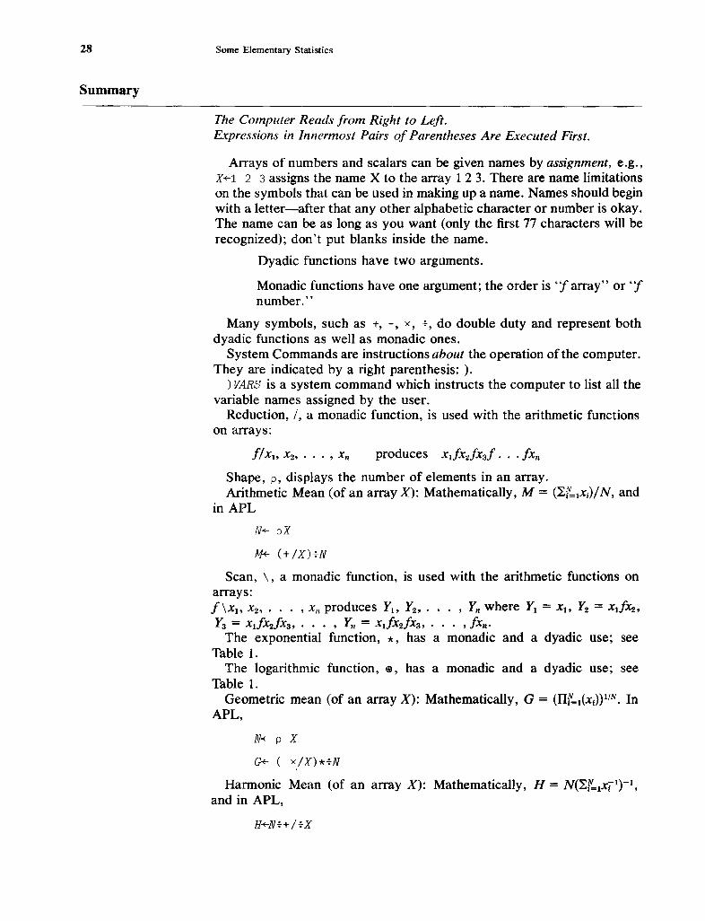
28
Summary
Some Elementary Statistics
The Computer Reads from Right to Left.Expressions in Innermost Pairs of Parentheses Are Executed First.
Arrays of numbers and scalars can be given names by assignment, e.g.,X+-l 2 3 assigns the name X to the array 1 2 3. There are name limitationson the symbols that can be used in making up a name. Names should beginwith a letter-after that any other alphabetic character or number is okay.The name can be as long as you want (only the first 77 characters will berecognized); don't put blanks inside the name.
Dyadic functions have two arguments.
Monadic functions have one argument; the order is '1 array" or'1number."
Many symbols, such as +, -, x, -;., do double duty and represent bothdyadic functions as well as monadic ones.
System Commands are instructions about the operation of the computer.They are indicated by a right parenthesis: ).
)VARS is a system command which instructs the computer to list all thevariable names assigned by the user.
Reduction, /, a monadic function, is used with the arithmetic functionson arrays:
produces xtfxzfxd... fXn
Shape, p, displays the number of elements in an array.Arithmetic Mean (of an array X): Mathematically, M = ('i.~=lXi)/N, and
in APL
N+- pX
Scan, \, a monadic function, is used with the arithmetic functions onarrays:f\Xh X2, ... ,Xn produces Y1 , Y2, , Yn where Yt = Xl> Y2 = XtfX2,Y3 = xtfx2 f x3, ... , Yn = XtfX2fx3, ,fxn •
The exponential function, *, has a monadic and a dyadic use; seeTable 1.
The logarithmic function, ~, has a monadic and a dyadic use; seeTable 1.
Geometric mean (of an array X): Mathematically, G = (I1~=l(Xi))1lN. InAPL,
N+- p X
G+- x/X)*+N
Harmonic Mean (of an array X): Mathematically, H = N('i.~=tXil)-l,
and in APL,
H+-N++/+X

Exercises 29
Exercises
Chapter 3
Sample Variance (of an array X): Mathematically, V = ~f=t (Xi - M)2/(N - 1), where M is the arithmetic mean. In APL,
V+- ( +/ (( X-M)*2»~N-_l
The Sample Standard Deviation (of an array X) is the square root of thesample variance.
Inner product (between two arrays X and Y of equal length): MathematicallY,IP == XtYt + X2Y2 + · . . + XnYn. In APL,
IP+-X+.xY
Mean (arithmetic) for Sample Proportions: Mathematically, MF == Lf<=lfriPRi' where K is the number of cells andfri is the relative frequency ofthe ith value of PR i , the ith sample proportion. In APL,
MF+FR+.xPR
Variance for Sample Proportions: Mathematically, VF = Lf=tfri(PRi - MF)2. In APL,
VF+FR+.x (PR-M)*2
How to continue entering data over more than one or two lines: use ,0 atthe end of a line of input on the terminal.
APL Practice
1. Let's explore the uses of the functions defined in this chapter.Let P+-3 and Y+-1&2&3&4.
(a) p P (e) p Y
(b) p 3 (f) p p y
(c) PP 3 (g) +/ Y and compare it carefully with +\Y
(d) p p P (h) (+ / Y~Y) which is the same as p Y. Why?
2. Assign the values 1&2&3&4 to X, the values -1& -2&-3&-4 to W, anddefine Z by Z+* X.
(a) 1*X (m) X*O
(b) X*1 (n) oeW
(c) 2*X (0) l~X
(d) X*2 (p) xe-l
(e) O*X (q) eZwhich is X
(f) x*o (r) +/X+ p X
(g) 7*W (8) ( +/X)+ p X
(h) X* -1 (t) What is the difference between (r) and (8)?
(i) lex (u) +/XxW*2 which is the same as X+. xW*2.
(j) X*l (v) -\Xand compare with-IX.
(k) 2f!'X (w) -\Wand compare with -IW.(I) xe2

30 Some Elementary Statistics
3. Evaluate the polynomialsf(x) == x 2- 5x + 6,f(x) == (x 5
- 1)(x2- 2),
andf(x) == x 4 - 3x2 + 2 for X+--5&-3 &-1 & O~~.1S2f:>3.
4. Practice the right to left rule by solving:
(a) 10+-3+-5 (t) -/1&2&3+3
(b) - 3 &-5 -10 (g) - / -;-1 - 3& - 2
(c) +3& -5&-10 (h) +\2-34
(d) 3-X-;-6-10 (i) +\10*123
(e) +/';-1&2&3
You should be able to find the answers without using the terminal andthen use the terminal to check.
5. Let the arrays X and y be defined by
X+-l&2&3&4&_ . . &10, Y+-2+X*.3.
Practice the algebra of summations by trying:
APL Form Math Form Explanation
(a) +/-i-X L i~111Xi the sum of the reciprocals of the elementsof X
(b) +/X-l L '~1 (Xi - 1) the sum of the differences Xi - 1(c) +/X*2 Li~l Xf the sum of the squares of the elements ofX
(d) (+/X)*2 (L i~l X i)2 the squared sum of the Xi(e) +/~X 2: i~l In Xi the sum of the natural log of the Xi (natural
log is log to base e)
(f) +/*X L i~l eX; the SUln of e raised to the powers Xi
(g) -IX L X:l (-l)i-IXi
(h) -j-X L i~l (-I)iXi
(i) +/Xxy Li~l XiYi { These sums occur very frequently in
U) +/YxX*2 Li~l XTYj regression analysis; see Chapter 8.
6. Verify that the first element of X is equal to the first element of + \X,while the last element of + \X is equal to +/ X.
7. Here are some more summation formulae. Try expressing each interms of APL functions.
(a) LjV=l Xi - 1(b) ~i"=l e x2i
(c) Li'::l (Xi + 3)2(d) Li'::t (-l)i(l/Xi)(e) ("LfJ=l X i)/N(f) l/"Lf=l (l/Xi)
(g) Li"=l eXT - 5)2(h) Show that Li~l kXi = k"Li"=1 Xi(i) Show that ~f=l (Xi + 2)2 = Lf"=l Xi2 + 2mr=1 Xi + N22
(j) Show that L~l (Xi - (Li"=1 X i )/N)2= Lf=l XT - 1/N('Li"=1 X i )2

Exercises 31
where N is the number of elements ofX. As there are several ways towrite each of the above, the suggested procedures in the solutions maynot always be the same as yours. You can, however, check that yourprocedure is correct by computing the numerical solutions. Use the listX defined in exercise number 5.
8. Interpret the following APL statements in mathematical form:
(a) +/fX (d) f+/fXxY
(b) -/fX (e) f+/ ( X-+/Xf p X)*2
(e) -/f-X (f) ( XxY)- ( +/X)x ( +/y)
9. Which of the following are invalid names?
(a) ABE LINCOLN
(b) B*
(e) LOUI$ THE 14TH
(d) xxx+yyy
(e) X1X2X3
(1) 2W+3Y
(g) IWILLBEHERETOMORROWATTHREE
Statistical Applications
I. When the elements of an array are ratios, the geometric mean may be amore useful measure of central location than the arithmetic mean wouldbe. If an array has elements that are rates of change, then the harmonicmean is usually preferable.
Consider the following data:
Year
196619671968196919701971197219731974197519761977
u.s. Total Residential Debt Outstandingin Billions of Dollars
274.2292.0312.8335.9357.8398.0454.5509.8549.8593.0655.0711.2 (estimated)
Source: U.S. League of Savings Association Publications #24,1977,p.28.
(a) Fil1d the arithmetic mean of U.S. residential debt outstandingduring the 12 years.
32 Some Elementary Statistics
(b) Find the ratio of each year's debt to the previous year's.(c) What is the geometric mean of these ratios?
(d) Find the percentage increase of the debt series from each year tothe next. (This is equal to the ratios in (b) minus 1.)
(e) What is the harmonic mean of the percentage increases?(f) What is the mean rate of growth in U.S. residential debt?
(g) Explain intuitively your answers to (a), (c), and (f).
2. In the following table CE represents the number of cracked eggs in acarton (each carton contains 12 eggs). CN is the number of cartons outof a sample of 60 cartons, randomly selected from a shipment of 2,000,that contain cracked eggs.
CE 1~_O 2__3 4__5__6__7__8 __9__1_0__11__12
CNl 0 5 7 11 16 8 4 5 2 0 0
(a) What is the average number of cracked eggs in each carton?
(b) What percentage of cartons have fewer than 2 cr::tcked eggs?
(c) On the basis of your answers to (a) and (b), shouid the shipment beaccepted? (A shipment is acceptable when 8% or less of the eggsare cracked.)
3. LetWhi= 1, ... ,5,takethevalues3,4,7,5,11,andYi =3+2Wi .
Find lV, Y, Sit, = (~f=t(Wi - W)2)/4, S} = (}:f=t(Yi - y)2)/4,Sw = VS¥;, Sy = YSf. Verify that iT = 3 + 2W, S} = 4S~, andSy = 2Sw.
4. Let r represent a list of estimates of the interest rate for next year: 5%,6%, 7%, 8%, 9%, 10%. Suppose we believe that the respective probabilities that these values will occur are 0.1, 0.2, 0.3, 0.2, 0.1, 0.1. Findthe expected value of the interest rate. What is the probability that theinterest rate will neither fall below 6% nor exceed 9%? (Note: theexpected value of a variable X which can take on only discrete valuesis defined by 'Lr=l XiPh where Pi is the probability that Xi will occur.)
5. Consider a gamble .wherein a fair coin is repeatedly tossed until a headturns up. If a head is obtained on the first toss the payoff is $2; it is $4 ifa head is obtained on the second toss, $8 on the third toss, and so on.Use the computer to find the expected return if the coin is tossed atmost a total of one hundred times. (A new wager is made after eachtime that a head appears.)

Exercises 33
6. The following measurements (in dollars rounded to the nearest integer)represent the increase (if positive) or decrease (if negative) in the dailyclosing price of General Motors and General Electric common stocksfor 10 consecutive days.
GM If---_2-----1__3 0 0 -_1 2__4 0_
GEl 3 4 -1 ° -1 -2 0 4 3 -2
(a) Which stock would you prefer with respect to average daily return?
(b) If the larger the variance of a security the larger the risk, which isthe riskier security?
7. Imagine yourself sitting at the roulette table in Las Vegas, having lostthe family fortune, and being left with only $200 at your disposal. Theroulette wheel will be spun about seventy more times before the tableis closed. There are 36 numbers and a double zero on the wheel. Youdecide to bet $3 on the number 11 repeatedly. The rule of the gameis as follows: If 11 comes up you get $105 ($3 x 35), the payoffis $35 for a $1 bet; if any other number comes up you lose the $3.What is your expected cash position at the end of the night?

4
How to WriteYour Own Function
In this chapter, after defining a few more APL expressions, we introducethe important concept of a fUl1ction which you can write yourself. At theend of this chapter your ability to apply APL will have taken a big leapforward. Let's press on.
4.1 The Sample Median
Sample Median
Residue, I
34
One measure of central tendency that is in widespread use is the median.The median is that value for which half of the sample values are less thanor equal to it and half are greater than or equal to it. The median for nobservations is defined mathematically by
M == ( (Xn/2 + x n/2+l)/2 if n is even (4.1)Xk' k == (n - 1)/2 + 1 if n is odd
where Xl :5 X2 ~ • • .:5 Xu are the order statistics obtained from n observations. That is, the n observations are reordered so that the smallestobservation is first (Xl) and the largest is last (xn).
Calculating M in APL might seem to be a formidable task, but in fact it isquite simple. In addition, calculating the median will introduce us to someuseful programming tools.
We have two problems to solve-discovering whether n is even or not,and reordering the array to get the order statistics. That is, we want anarray with the smallest observed number first, the largest last, and witheach number less than or equal to the number on its right. Let us begin withsome useful new APL tools.
The Residue Function
The first of these tools is the residue function, I, which is upper shift M.
The residue function applied to two numbers A and B, denoted by A IB,

4. 1 The Sample Median 35
Absolute Value, I
yields the A residue of B, and is the "remainder" left over after dividing Ainto B. For example, the 2 residue of 3 is 1, the 3 residue of 8 is 2, the 4
residue of 8 is 0, and so on. Of particular interest is the 1 residue of apositive decimal number; thus
11 2 . 5&°.6&4.0
0.5 0.6 0
In other words, the 1 residue of a positive decimal number is simply thedecimal fraction of that number. Let's try some more examples:
31 0 1 2 3 4 5 6 7 8 9 10
o 1 2 0 1 2 0 1 201
101 11&102&1032&11021
1 2 2 1
11 6.0&-6.4&-0.3
° 0.6 0.7
21 3&4.°&-3.°&6.2&-6.2&-4.0
1 0 1 0.2 1.8 0
3/4.0&-4.0&5.0&-5.0&4.2&-4.2&-4.8
1 2 2 1 1.2 1.8 1.2
The results for the first two arrays are clear enough, but what about theothers? Close inspection reveals a difficulty in interpretation of the resultsonly when we try to get the residue of a negative number. What is occurringwith negative nUlnbers will become clear as soon as we understand theresidue operation with positive numbers.
If we look back at the first example we notice a recurring sequence 0 1 2.Suppose that we extend the array to include negative numbers, say
31 -10 -9 -8 7 6 5 4 3 2 1 0 1 2 3 4 5 6 7 8 9 10
2 0 120 120 1 2 0 1 2 0 1 2 0 1 201
Note that the pattern is exactly the same.However, 314 is 1 and 31-4 is 2, so the result is not simply the residue of
the absolute value of the righthand list. In fact the monadic use of the Isymbol is the absolute value function. For example
4

36
Absolute Value andResidue to ComputeFractional Parts ofPositive & NegativeNumbers
Logic of ResidueFunction
How to Write Your Own Function
So we could find the fractional parts of elements of a vector that had bothpositive and negative elements by
111-2.1 -1 0 1.2 3.1
0.1&0&0&0.2&0.1
Remember, we proceed from right to left, first finding the absolute valuesof the array by using the monadic I function and then using the dyadic Ifunction to find the fractional parts.
While we ·have shown that the residue is consistent in its operation onpositive and negative numbers, we need to explain the logic behind thisconsistency. Here is one way to think about it. The residue for a positiverighthand argument is obtained by successively subtracting the lefthandvalue until the result is less than the lefthand value. If we have 317 wesubtract 3 from 7, yielding 4 , then subtract 3 from 4 , leaving 1, which is lessthan 3 so we stop. The last value is the residue. When the righthand valueis negative we add the lefthand value to the right until the result is positive.So if we have 3/-7, we add 3 to -7, yielding -4, then add 3 to -4) leaving-1, then add 3 to -1 to get 2. This process defines the residue function forpositive lefthand and negative righthand values.
Finally, here is a diagram of the results of the first example:
Statement 31 -10 - 9 8 7 6 5 2 0 2 3 5 6 7 8 9 104 3 1 1 4Result 2 0 1 2 ° 1 2 0 1 2 0 1 2 0 1 2 0 1 2 0 1Index 1 2 3 4 5 6 7 8 9 10 11 12 13 14 15 16 17 18 19 20 21
Diagram 1 Illustrating the Value of the Residue When Dividing Numbers by Three*
Residue = 2 4 7 10 13 16 19 22
Residue = 1
Residue = 0
* Right argument of residue on x axis, residue on y axis, numbered points are the index values (seeabove), Locate 4 on the bottom of the diagram, move vertically until you cross the diagonal line, readthe residual value 1 on the left. Check to see that it is element 15.
Arrays: Parity
Parity of the Number of Elements in an Array
After this lengthy digression we can take the first step in finding themedian. Does the array have an even or odd number of elements? If you

4. 1 The Sample Median 37
Ordering Arrays
Indexing Arrays
have re-Iogged-on to do this chapter, yOll will have lost the X and Yarraysdefined in Chapter 3. If so, please enter these values first:
X+1&2&-3&-4&5&-6&-7
Y+2&4&6&8&4&2&6
Solution:
N+ 0 X
21N
If the result is 0 we have an even number of elements (N is divisible by 2
with no remainder), and if the result is 1 we have an odd number. In ourexample N is 7, so we have an odd number and the result of 2/ N is 1. Youmay be wondering why we bother with all of this, since printing N tells usimmediately if N is even or odd. The reason is that we are laying thefoundation for the computer to make the decision itself, without our intervention.
Ordering the Elements of an Array
The next problem is to reorder the array X so that the smallest element isfirst and the largest is last. To be safe and not lose the original order, let usstore the reordered array X in a new array called R. The process of reordering an array introduces two new concepts, the grade up (or down) functionand the simple mysteries of indexing. Let us first consider the indexing ofarrays and the indexing function.
Since a one-dimensional array is merely a list of elements, it seemsnatural to give the position of each element in the list an index value and tolet that value be the position of the element in the list; in short, the firstelement going from left to right is element number 1, the second is number2, and so on., APL lets us refer to the elements in an array in a simplemanner. Type out the following:
W+9&10&3&8&12&0&1&5
W
9 10 3 8 12 015
W[1]
9
W[5]
12
W[1&2&3]
9 10 3
W[3&1&2]

38
INDEX ERROR
Grade Up ~
Grade Down'
How to Write Your Own Function
3 9 10
w
9 10 3 8 12 0 1 5
The examples illustrate what is happening. The indexing of an array allows'you to select from an array the individual elements of an array in anyorder. In addition, specific elements in an array can be replaced veryeasily; for example,
9 8
6 10 3 15 12 0 1 5
The contents of [ ] can be any valid APL expression, provided only that itresults in an array of integers, none of which is larger than p W, the numberof elements in the array W. Try
W[O]
INDEX ERROR
W[o]
1\
W[2 2 2J
10 10 10
f,y[ 9 J
INDEX ERROR
Wf9]
1\
WC-2]
INDEX ERROR
W[-2]
1\
Now consider the functions grade up, th, and grade down, t. Each isformed by typing one character on top of another (the I we used forresidue (upper shift M), backspace, and then upper shift H for 6 (delta) or Gfor V (del». Let's try it on the array W that we defined above:
~w
6 7 381 254

4. 1 The Sample Median
and
39
4 5 2 1 8 376
To see what is happening here, write down the elements of W with theirindices underneath them:
W: 6index: 1
10 32 3
15 12 0 1 54 567 8
Sorting an Array
Sample Median
We see that ~ (grade up) gives us a new array in which the first element isthe index value of the smallest element of W, the second element is theindex value of the second smallest element of W, and so on. Grade down(t) also indicates the order of the array, except that the first index value inthe new array is that of the largest element in W, the next is the index valueof the second largest element of W, etc. The last index value in the newarray is the position of the smallest element of W.
You might be able to guess what we should do now in order to get anarray with the elements of Wor X or Y listed in either ascending or descending order. Try
WUP+-W[~W]
WUP
o 1 3 5 6 10 12 15
WDOWN+-W[ 'fW]
WDOWN
15 12 10 6 5 3 1 0
This is all you need to sort any list of numbers. The grade function ordersthe index values inside the square brackets, and then the elements represented by those positions are selected.
Calculation of the Sample Median
Now we can calculate the median. If our expression for discovering theparity ofN tells us that N is odd, then by Eq. (4.1) the median value of theelements ofX is element number «N - 1)/2) + 1 of the ordered array. (Itis irrelevant here whether the elements ofX are arranged in ascending ordescending order.) Let's try it, but first let's recall what X and N are.
X
1 2 345 6 7
N
7

40 How to Write Your Own Function
XUP+-X[4X]
M+XUP[l+ (N-l)~2J
M
3
If N is even; the median is:
w
6 10 3 15 12 0 1 5
WUP+-W[~WJ
K+- (p W)~2
M+-WUPCK ,K+l]
M-E- ( +/ M) ~ 2
M
5.5
<E- rearranges X in ascending orderand stores result in xUP
<E- picks out the middle elementof xup
<E- picks out the middle pair ofelements
<E- averages them
Catenate, ,
You can easily check by visual inspection that both calculations arecorrect. Each of these two sets of APL statements can be called a "routine' , ; a routine is a group of APL statements that perform some operation.
These two APL routines worked, but the third line in the second routinecontains something strange-the contents of [ ] must be an array of integers, but what is the comma doing there? Why does WUP[K,K + 1] work?First, ask yourself what you would get if you typed in K &K + 1, where Khas the value 4. If you incorrectly read from right to left, you might believethat the answer would be 5 5. You would be incorrect in believing that KK + 1 is computed as "to the array K &K add 1." APL expressions arecomputed from right to left. But we cannot separate K and K + 1 byparentheses alone, e.g., K (K + 1), since APL expects a function to appear between K and (K + 1). The function represented by " ," is discussednext.
The Catenate Function
The solution to our little problem introduces a very useful concept and auseful function, the catenate function " :', which is keyed in by typing acomma. The catenate function enables us to extend an array or to makearrays out of scalars. For example, let A and B denote arrays of length pand q, respectively, and let K and L be scalars. Then

4.2 The Function Definition 41
A,B produces an array of length (p + q) with the A elementscoming first,
B,A produces an array of the same length, but the B elementscome first,
A,K produces an array of length (p + 1),K,L produces an array of length 2,
,L produces an array of length 1.
So the solution to our problem is to create the array K,K + 1, a twoelement array of which the first element is K and the second is K + 1.
We have now solved the problem of computing the median but, especially ifN is even, it is a nuisance to type out all these statements each timewe want the median. What would be convenient would be a functioncalled, say, MD, such that typing MD&X (where X is an array) produces themedian of X. In short, we need a monadic function just like the onesprovided by APL, like 4, p, f, and so on. To meet this need, APL providesa method whereby the user can supplement the set of primitive APL functions (those available from the keyboard, such as *, +, etc.) with userdefined functions. Once the user function is defined, it can be used overand over again just by calling it-for example, by typing MD~X, where X isan array, the median of which is defined by the function called MD.
4.2 Function Definition
Entering FunctionDefinition Mode
'l
Niladic Function
Our first step is to tell the computer that we want to define a function tobe used later. This is done by typing 'l (called "del"), which is the uppershift Gkey. We will also need to inform the computer when we are finisheddefining the new function. That is done by typing in V again. Thus thecomputer expects that between the two V symbols it will be receivinginstructions that will define a new function.
Certain rules must be followed when defining functions, and we willconsider these rules now. If we type v, which tells the computer" Functiondefinition coming up," our next action must be to give the function a name.Once we have named our function, both we and the computer can refer toit even while we are in the process of defining it. But in APL we not onlyname a function, we can also give it some arguments-that is, somethingfor the function to operate on.
Niladic Functions
In §3.2 we defined monadic and dyadic functions-functions with oneand two arguments, respectively. We can also have niladic functions,which do not have any arguments. A niladic function is called simply bytyping 'V and the name of the function and hitting the EXECUTE or RETURN key. It then carries out the procedure specified in the functionyou do not give it any arguments to work on. Let's consider an example.
42
) CLEAR
Roll?
CorrectingTyping Mistakes
How to Write Your Own Function
Suppose we want to run some experiments on the computer to check out/'.:.
the statistical properties of the probability estimator PR discussed at theend of the last chapter. One of the first things we have to be able to do is togenerate data similar to that which we would get from rolling a pair of dice.IfN, the sample size, is 16 or 20, and NN, the number of repetitions of theexperiment, is 100 or more, and if we want to see how the mean andvariance change as we alter N, then we are facing a very large amount ofdice throwing. Such an activity may not be your favorite way of spending aSunday afternoon in the sun, but if it is pouring rain, go ahead and roll thedice. Fortunately instead of rolling dice we can use the computer to simulate the process of actually tossing them. So, let's generate some data.
We begin by defining a function that will give us one roll of a pair of dice.Before beginning to define our own functions, let us clear the decks, so tospeak, of any other nonprimitive functions that might be already in our"workspace" and might give us some difficulties and strange responses.We do this by typing )CLEAR, and the computer responds by telling us thatour workspace (you can think of it as the part of the computer that we areusing) is clear. WS stands for workspace. You will recall that the symbol )indicates that a system command is coming up. Type
)CLEAR
CLEAR WS
\JR+DICE
[1J
The use of Vin the first line is clear enough; it tells the computer that weare defining a function. In more technical language, it puts us into "function definition mode" instead of "execution mode." The word DICE is thename of our function, but why R? We will explain that one in a minute.
The computer responded with a [1]. This is its way of telling you that itunderstands that you are defining a function, and [1 J is the number of thefirst statement for you to write. The computer now expects you to write anAPL statement, so let's oblige. We will be using a special APL symbol, ?,called roll, which is upper case Q. Be careful not to get confused. Someterminals have two? symbols, one for APL and one for non-APL use. Ifyou are unsure about which is correct, just experiment-you can't hurt athing. Starting directly to the right of [1 J, type in
[lJ R++/?6 & 6
and then hit (but only after checking line [1] very carefully to see if it iscorrect) EXECUTE. The computer will respond with [2J and you type V
[2J \J
Then hit EXECUTE (or RETURN on some terminals) again.If you made a mistake on line [1 J, and you noticed it after pressing
EXECUTE, then you can correct it very easily by typing in on line [2 ]
[2J[1J R++/?6 6
4.2 The Function Definition 43
Generating RandomNumbers
FunctionHeaders
In short, you repeat the line number of the incorrect line and type in what itshould be.
We have defined our function, but what is it? Type
DICE
6
DICE
7
DICE
3
Generating Random Numbers
By now you have guessed that DICE is a function designed to give youthe result of rolling a pair of dice. The basic element in the function is theprimitive function roll, for which the symbol is ? . Typing
?6
5
produces a random number between 1and 6, typing ?10, a random numberbetween 1 and 10, and in general ?N produces a random number between 1and N. The probability of anyone specific number showing up is 1/N. Thisis the monadic use of the aptly named roll function. Now we see why? 6&6produces two numbers from 1 to 6, each of which is equally likely to occur;this is the computer's simulation of rolling a pair of dice.
Our statement number [1] is now clear:? 6 6 gives us an array of tworandom numbers (statistically independent in fact), and + /? '6 6 gives usthe sum of the two random numbers.
Function Headers
We are now ready to answer the question about the function header-theline that defines the function. (In this case the function header is 'VR+-DICE.)In line [1J, instead of writing R++/? 6. 6, we could have written:+/? 6 6. What's the difference? In either case, calling DICE produces thedesired result in that the computer prints out the sum of a random tossingof two "computer dice."
The distinction between the two statements becomes apparent when weconsider whether we want to use the result in some other APL statement.For example, we might wish to calculate DICE+2. Alternatively, we mightwant a function such that when the user types HI, the computer respondsWHAT IS YOUR NAME. Now we do not want to use such a function in anything else; we just want the computer to type out WHAT IS YOUR NAME.

44
InteractiveProgramming
How to Write Your Own Function
The DICE function is said to "return an explicit result," something wecan use elsewhere .. and the HI function does not produce an explicit result.If you want an explicit result, you need the header in this form: V (SomeVariable Name) +- (Name of Function). Somewhere in your function youwill produce the explicit result that you want; that result must be storedunder the same variable name as that used in the header. This is whatwe did in VICE. If instead of using R in the header we had writtenVD+-DICE, then litle [1] would have to read
[lJ D++/? 6 6
The Quote Function
To provide a contrasting example of a no explicit result function, considerthe function HI mentioned above. Let's define HI:
Quote'
'VHI
[1] 'WHAT IS YOUR NAME?'
[2J V
Now try typing
HI
WHAT IS YOUR NAME?
~ quote is upper shift K
~ you type
~ computer responds
Monadic FunctionHeaders
This example introduces another useful APL function, the quote ('),upper shift K. The characters between the quote signs are treated as justthat: characters. When the computer comes across a line like [lJ when inexecution mode, it simply prints what it sees.
Monadic Function Headers
Let's return to functions with arguments. First, the header of a monadic(sitlgle argument) function is of the form
opens--------~) VM+-MD X ....(--------"dummy"function variable name
returns anexplicit result
functionname
Why is X in the above header to the function MD called a "dummy" variablename? The reason is that in the header, X represents the argument that thefunction is supposed to operate on, and X appears later in the body of thefunction. But when you use the function MD on a variable V, or a variable P,or A, you would simply type in MD V, or MD P, or MD A.
Remember the median? We showed how to calculate it on page 40. Nowwe know how to make it a function. First, we need to decide on a name;

4.2 The Function Definition 45
UnconditionalBranch -+
Line Labels
ConditionalBranches
MD seems to be as good as any. Second, we need to decide whether wewant an explicit result or not. Presumably, since the median IS going to beused in some other calculations by someone at some time, it would be bestto have it return an explicit result. Third, do we want the function tohave arguments? Well, the answer to that is that if we have a vector, say X,in the computer we might want its median, and an easy way to say that is'MD X', so we want a monadic function. Recall that our first task is to enablethe computer to decide whether X has an odd or an eve·n number of elements in it (see page 40). But, somewhat more importantly, we want thecomputer to decide which way to calculate the median on the basis ofwhether N is even or odd. In short, we want the computer to do onecomputation if N is even and to branch to another computation if N is odd.As you might guess, this is a not so subtle hint that we are about to define anew APL operation; this one is called ~ ~branching."
Unconditional Branch
Suppose that in some APL routine you want the computer to go directlyto line 6 if it gets to line 3. This is easily done by entering +6 on line 3.
[ 3J-+6
The symbol -+ is the upper shift of the + key. This is called ~ ~unconditional
branch." In this case, the computer would know that if it ever gets to line 3it must go directly to line 6 and execute it next.
Now for reasons that will become apparent in Chapter 7, it is a good ideato develop the habit of giving labels to lines to which the branch directs thecomputer to go. So if we label line 6 "SIX", for example, then the statement on line 3 could read [3 J-+SIX. In this case line 6 would look like this:
[6J Sl"X: {some APL instruction to be performed}
The computer reads from right to left, so when it encounters the symbolin a line of a routine, it knows that everything to the left of : js the labelfor this line of instruction in the routine. We have simply named the lineSIX. It now has a position number [6 J, and a label or name, SIX.
Let us now discover how to solve our problem. Recall the two ways inwhich we calculated the median (page 40). What we want to do is to go toone set of instructions or the other, depending on whether N is odd or even,and then to exit from the function. Let's see if we can program the following steps:
(a) determine whether N is even or odd;
(b) if Nis odd, continue with the "odd" calculation and then exit from thefunction;
(c) if N is even, branch to the "even" calculation and then leave thefunction.

Index Generator, 1
RANK ERROR
How to Write Your Own Function
Consider (but do not type anything yet!):
'iJ M+-MD X
[1J N+ p X
[2J -+oDDx 12/N
The last part of this line is clear enough: 2 /N produces 0 if N is even and 1if N is odd, since 2 IN is the "two" residue of N, but what can we make ofthe first part? Let's look at the next section.
The Index Generator
The symbol 1 is the "index generator" (upper shift I). For any integer N,IN produces the "index array" 1, 2, ... ,N. 1.1 produces an array withonly one element in it, namely 1. But what about 10 ? This produces an"array" with nothing in it! The index generator, the monadic use of 1,
unlike most of the other primitive functions in APL, cannot operate on anarray; e.g., lA , where A is an array, produces the result RANK ERROR.
Conditional Branches
If N is odd, __ IN produces 1, so line [1] produces an array of length 1with a 1 in it, and multiplying- this by ODD produces ODD. The first part ofthe statement says: Branch to the line labelled ODD. But what if N is even?Then 1 2 IN gives an array with nothing in it, and ODD multiplied by thatproduces an array with nothing in it still. APL interprets -+(an array withnothing in it) as "ignore this silly statement and continue to the next line."So we have in line 2 a conditional branch statement; go to the line labelledODD if N is odd, otherwise continue. So let us begin and put down thecomplete function. If you make a mistake typing any line, remember howto correct it: backspace to the beginning of the error and hit the linefeed orATTN key, depending upon the type of terminal and computer system thatyou are using. On most CRT screens you just backspace and reenter theline.
'J M+MD X
[1J N+ p X
[2J XUP+-X[~xJ
[3J -*ODDx 12}N
[4J K+ (p X)+2
[5J M+(+/XUP[K~K-1J)';'2
[6J -+0
~if N is even, calculates Mfor even case, otherwise goesto line ODD
~tells computer to leave function

4.2 The Function Definition
[7J ODD:~XUP[1+(N-1)f2J
[8J
oE- if N is odd, calculates Mfor odd case and thenleaves function
47
Exit from Function
Correctinga Defined Function
Hold it!Before typing the final 'V and completing the function definition, check
your entries very carefully. If a line has an error in it, then enter its linenumber (in brackets), type the correct version of the line, and hit RETURN. The computer will respond with the line numbers following the oneyou entered. If there are no more corrections, type in "J and RETURN;otherwise repeat the process.
The first and third lines we have figured out. The three lines [2], [4],
and [5] are copied from page 40, where we wrote down the routine forcalculating the median M when N is e.ven. But line 6 is a puzzle. Noticethat the header of the function has no line number, and that line numbersstart with 1. The function ~O, or-+(any line number not in function) tells thecomputer to "exit" from the function and go back to the point from whichour function, MD, was called. In short, when the computer hits line 6 itknows it has finished calculating the median. It is best to stick to "-+0" toexit from the function, since you may later want to add new lines to thefunction. The last two lines are modified from page 40, where we showedhow to calculate the median where N is odd.
Let us tryout our new median function. We put into the computer the Xand Warrays we used earlier:
X+l 2 3 -4 5 6 7
W+6 10 6 15 12 0 1 5
and now we can check the function out.
MD X
3
MD W
5.5
Correcting a Defined Function
What if you enter MD X and you do not get -3? You've made a mistake!Let's see how to correct it. First, relist the variables X and wand make surethat they are correct. If they are, continue; if not, redefine X or wand retrythe function.
But suppose you are sure the mistake is in the function MD? In order tocheck it, you will need to display it. To do this, we type in:

48
Display, 0
How to Write Your Own Function
\J MD[OJ \J
V M+MD X
[1J N+p X
[ 2] XUP+X[ ~xJ
[3J -+ODD x 121N
[4J K+(p X)-i-2
[5J ~(+/XUP[K,K+1J)+2
[6J -+0
[7J ODD:M+XUP[1+(N-1)+2J
-E- this line "opens" the function,displays it (that's what [OJ does),and closes it. D is typed in byupper case L.
<E- this is the computer's responseto your command to display thefunction
V
Suppose you discover that you made some typing errors in the function.In Chapter 5 we will show you in detail how to correct errors, but for nowwe will give you one drastic, but surefire, way to do it. If we remove thefunction altogether, we can completely redo it-this time very carefully.To remove the function, type
)ERASE Command )ERASE MD
SI DAMAGE <E- this statement is the computer'sresponse. It warns you that youhave erased a suspended function.SI stands for State Indicator.
Suspended Functions
You might also get a statement indicating there is a syntax, value, orsome other error in a line of your function when you try to execute thefunction with an error in it. For example,
MD X
VALUE ERROR
MD[1JN+RX
.- this is the computer's responsetelling you the first line andfirst position of your firstmistake
Removing aSuspendedFunction
)SI Command
The result of this error is to prevent further execution of the function. It issaid to be suspended. At this time, it is best to remove the suspension. Thisis easy-type
.- this is upper case "+"
In order to check whether you have cleared the suspension, type
)SI

Summary 49
Summary
If you get no apparent response (actually a blank line) all is well. But ifyouget something like
MD[3]*
type in the -+ instruction again. Keep doing this until you get a blankresponse to the system command )SI.
Now erase the incorrect function and start again. Remember, you cannot correct the function simply by redefining it unless you first erase theold function. (This is not strictly correct-you could do it if you gave thecorrect function a new name (i.e., one that differs from the old name).)
One last word: if you think that the MD function is a lot of fuss about asimple operation, you're right. Later on we will show you how to calculatethe median in one short line. But in writing out the routine MD you learned alot about APL that will be very useful in the following chapters, and that,of course, is what this book is all about.
Sample Median, M (of an array X): that value such that half theobservations in X are less than or equal to M and half are greater or equalto it.
Residue function, I: in its dyadic form it is written AlB. For positive values of A and B, the A residue of B is the remainder of dividing BbyA.The monadic use of I yields the absolute value.
Indexing, [I] (of an array X): elements of an array X can beselected by specifying their position in the array; the positions are labelledfrom 1 to pX starting from the left. X[I] gives the value of the number inthe array X in the Ith position from the left.
Grade up, ~ (upper shift M, backspace, upper shift H) (of an arrayx): gives an array, the first element of which is the index position of thesmallest number in X, the second element is the index of the next largest,and so on.
Grade down, ~ (upper shift M, backspace, upper shift G) (of anarray X): gives an array, the first element of which is the index position ofthe largest number in x, the second element is the index position of thenext smallest, and so on.
Catenate, "," (the comma): forms one array out of its arguments;A,B is an array with the elements of A listed first where A or B can be anyone-dimensional array or scalar.
Roll, ? (upper case Q): ?N, where N is all integer that generates arandom integer from 1 to N with probability liN.
Index Generator, 1 (upper shift I): monadic function, IN, N aninteger, produces the "index" array 1, 2, 3, . . . ,N.

so How to Write Your Own Function
Quote, ' (upper shift K): all keyed entries between a pair ofquotes are treated as characters and not executed as APL functions.
Del, V (upper shift G): the instruction that is used when enteringor exiting from function definition mode.
Niladic function: a function which has no arguments; it carriesout a specified procedure when called.
Function Headers: first line of a function that gives the functionname; specifies whether function produces an explicit result or not, andcontains either zero, one, or two arguments. Thus:
\J HI
\J A GO B
\J R+-FNC
V R~FNC X
niladic (no argument) function, noexplicit result produced
dyadic function, no explicit resultproduced
niladic function, explicit resultproduced
monadic function, explicit resultproduced
(All six combinations are possible)
In function definition mode, a line in a function can be corrected bytyping in the line number and the correct version of the whole line. Forexample, in correcting line [1 J at line [3], you would type: [ 3] [1] (correct APL statement).
Unconditional Branch, -+: used within a function to alter execution path to a different line. Thus:
[3J -+6
or
[3J -+LABEL
[7] LABEL: (an APL expression)
Line Label: a name for a line in a function. When the second of theabove versions of line 3 is executed, the next line to be executed will benumber 7 with the label LABEL rather than number 4.
Conditional Branch: branching to a function line on the basis ofthe "condition" of some APL expression. Example:
[3J -+TRUEx l2/N
[4J 'THE CONDITION IS FALSE'
[6 J TRUE: (another APL expression)

Exercises 51
Exercises
If 21 N takes the value 1, the next executable statement is line [6] labelledTRUE. If 2 IN takes the value 0, next executable statement is [4].
Quad, 0 (upper shift L): when used as illustrated below with thefunction MD it displays the function MD:
V MD[OJ V
)CLEAR: a system command used to remove all existing functionsand variables from the existing workspace. The workspace can be thoughtof as the part of the computer which is assigned to the user for his computation procedures (both stored data and functions).
)ERASE: (FUNCTION NAME): a system command that enables you toerase a function from your workspace.
)SI: system command called state indicator. If you have functions which cannot complete their operation, they are said to be suspended. The command )SI will indicate which functions are suspendedand at what line in the function the suspension occurs.
To clear a suspended function, type -+ as often as needed to get a blankresponse from the command )SI.
APL Practice
1. Let's examine in some detail the use of the new APL functions presented in this chapter. For X+-5+ t 11, compare the results of the operations in each question.
(a) 1 IX (j) X[ t 2 J+-O & 0 and then ask for X
(b) 0 IX (k) X[ 1 1 2 3 J(c) 2 IX (1) X[ t 4 J(d) -2\ X (m) X[1VX] and compare to X[ t pX]
(e) 10 Ix (n) X[O]
(f) X I0 (0 ) X[ 1 2 ]
(g) XI-10 (p) P+t4and then X[P]
(h) X[t3J (q) xiX(i) X[ 2 , 3]
2. Since you know that the meaning of?6 6 and 6 6 is equivalent to 2p6,
why not combine them into ? 2 p 6 ? Try:
(a) ?3 p 6
(b) ?3 p 0
(c) ? 3 p 1
(d) ?i p 1

52 How to Write Your Own Function
(e) What is the difference between 3 p?6 and (a)?
(f) What is the difference between pX,p Y ., (pX),( p Y) and pX, Y for anyarrays X and Y?
3. Indexing can be used with the variables defined as a list of characters.Consider the following code game. Let
AL+'I WILL MEET YOU TOMORROW AT SEVEN'
(a) AL[8 26 22 26J tells whom you will meet
(b) AL [ 22 ., 9 , 29 , 1 7 ., 26 ., 15 , 22 ., 26 ., 33 ., 17] tells where
(c) AL[10.,26, 27J says what you will do
(d) AL[29,30,31,32,33]+'SIX'changes the time of the meeting
4. Let Z+-5+ 111
(a) (( 6 p1 ) ., ( 5 pO)) / z: picks the six first elements of Z, and is equivalent to Z[ 1 6] .
(b) Show how to pick the last four elements of Z.
(c) For any array Z write an APL expression that will pick the middlenelements. What if pZ is even?
(d) Is 2[1'1'ZJ equal toZ[~4ZJ?
(e) Suppose you want to delete the seventh element of Z. How wouldyou ask the computer?
5. Can you discover, with the computer's help, which of the followingseries converge to a limit and which diverge? If the series converges,can you determine what the limit is? How accurate is your answer?Compare your result with a table of limits of series.
111(a) 1 - "2 + "3 - 4"" ..
12345(b) "2 + 3 + 4 + "5 + "6 + " · .
50 51 52 53 54(c) T + T + "2 + T + 4 + · " .
111 1(d) 20 + 22 + 23 + 24 + . · ·
1 234(e) 2.3 + 3.4 + 4.5 + 5.6 + · · "(f) e-1 + e-2 + e-3 + e-4 + · · ·
(g) (1 + +r+ (1 + -}r+ ( 1 + {r +. . .
4 5 6 7(h) 2.3 + 3.4 + 4.5 + 5.6 + . · ·
(i) (-1)1 (_1_)1 + (_1)2 (_1_)2 + (_1)3 (_1_)3 + ...1 + 1 2 + 1 3 + 1
(j) 1· In (1 + f) + 2 · In ( 1 + }) + 3 . In (1 + }) + · · .

Exercises S3
e 1 e2 e3 e4
(k) f+T + f+l + 3+1 + 4+1 + · · ·
log 1 log 2 log 3(1) 1 + log 1 + 2 + log 2 + 3 + log 3 + · · ·
6. Let the list M ~ 3 3.2 3.5 3.6 3.6 3.7 4 4.2 4.5 5.1 5.3 5.5 representthe annual U.S. money supply in hundred billions of dollars for a 12year period. Define a new list consisting of the first differences of theelements of M. That is, for i = 2, 3, , 12, let DMi = M i -
M i - 1 = 3.2 - 3, 3.5 - 3.2, 3.6 - 3.5, , eleven terms in total.What are the mean and variance? How about the list (Mi - Mi-t)1M i - t , i = 2, 3, ... , 12? The list log Mi-t/log M i , i = 2, ... , 12?
(Hint: One suggestion for finding the first differences of a list is:
'V DM+-DEF X;Ml;M2
[1J M1+ (O,«pM)-l)pl)M
[2J M2+ ((((pM)-l)pl)p,O)p/M
[3J DM+-M2-Ml
[4J \J
Notice that DMl+-DEF M produces the first differences of M.DM2+-DEF DMl would produce the second differences of M,DM3+-DEF DM2 would produce the third differences of M, and so on.What are the mean values of the differences DM1, DM2, DM3 • • .?)
7. Here are some important inequalities and identities.(a) The Cauchy-Schwarz inequality
(Lf=lXiyi) :5 (Lf=txr)(Lf=tyr)
(b) Holder's inequality
(Lf=tXiYi) ~ (~~lxf)l/P(Lf=ly?)l/q
for any p and q such that lip + l/q = 1, p > 1.
(c) Minkowski's inequality
[Lf=l(Xi + Yi)K]l/K :5 (~f=lXf)l/K + c~:r=tyf)l/K
for XiYi ~ 0 and K > 1(d) For Lf=lai and Lf=lbi convergent series of positive numbers such
that Lai ~'Lbi' we have
}:i"=lailog(bi / ai) :5 0
(e) The Lagrange identity
(Lf=txr) (Lf=lYT) - (}:f=lXiYi)2 = ~r<j(XiYj - XjYi)2
In some advanced statistics courses, these inequalities and identitiesare proven by algebraic methods. However, here is a way to use the

54 How to Write Your Own Function
computer to be fairly certain that the result can be proven algebraically.
Pick four integers at random (Hint: use ?); say you get 49 10 15. Foreach integer pick a random sample ofnumbers for listx and another fora list y, where the number of elements in each list is in tUfn 4 9 10 15.Check to see that the suggested inequalities hold with each sample.Repeat the same experiment using different random lists x and y eachtime.
If you discover no reversal of the inequalities (or violation of theidentity), you may reasonably suspect that the result can be provenalgebraically, and hence that it is a mathematically correct statement.
The above procedure is known as a "sampling experiment," andprovides the basis for what are known as 4'Monte Carlo" procedures.Monte Carlo procedures often are used to solve mathematical problems that are difficult to solve by analysis.
8. Enter the function MD X (page 48) into your workspace.
(a) Display the function.
(b) Describe what the function instructs the computer to do at line [3].
(c) Add the line 4The Median of X is' between lines [5] and [6].
(d) Execute the function and press the ATTN key before you get anyanswer (i.e., while the computer is in execution mode). Press thecommand )SI .
(e) Get out of the suspension.
(f) What would the comp~terdo if you changed line number [6] of theoriginal function into -+1 and the number of elements in X is even?
Statistical Exercises
1. Let C<E--t + ?100 p 2 represent the outcome from tossing a coin 100times. The random variable C takes on the value 0 if a "head" and 1 ifa "tail." If a head occurs you win one dollar, while if a tail occurs youlose one dollar. Calculate how many dollars you expect to win or loseif you play this game with the computer. Try it four times. What wouldyou pay to play this game?
2. The standard deviation of the binomial distribution with parameters nandp is given by the formula S = Vnp(1 - p), where n is the samplesize and p is the probability of success in a single trial. For n +- 100and p ~ (LI0) -7- 10 find the value of p for which S is maximum. Isthere a minimum?
3. Your friend from Texas called you up and asked you to find out whatthe average price is of used cars sold in N.Y. You collect a smallsample of New York used car prices as shown in the following table.

Exercises
p
F
2.5
o3
2
3.5
5
4 4.5
4 6
5
15
5.5
14
6
18
6.5 7 7.5 8
11 8 9 4
S5
8.5 9
3 3
P is the price of the car in thousands of dollars rounded to the nearest0.5 thousand, and F is the frequency, i.e., how many cars you observed at each respective price. You have a sample size of 102. Calculate the sample mean, variance, and standard deviation. Plot the histogram of P vs. F. How would you convey to your friend, who doesnot know any statistical theory, the information you have collected?How would you advise her?
4. One hundred cans of floor wax, randomly selected from a large production lot, have the following net weight in ounces with the corresponding frequencies:
weight
frequency
19 19.2 19.4 19.6 19.8 20 20.2 20.4 20.6 20.8 21
o 3 8 9 16 20 15 12 4 5 6
(a) Find the sample mean weight (x).
(b) Find the sample median (Mx) and compare its value to the mean.Explain the difference.
(c) What is the value of the sample standard deviation S?
(d) What percentage of the sample falls into each of the followingintervals:
1. i ± IS2. i ± 2S3. i ± 3S
(e) The variation in production by net weight is "acceptable" whenthe mean value is 20 ounces and 95% of the cans produced containno more than 20.3 nor less than 19.7 ounces. Can we conclude thatthe production run is acceptable on the basis of this sample?
5. The formula P(Yi) = (0.1) (y + 1) gives the probability of y = 0, 1, 2, 3occurring.(a) Graph P(Yi).
(b) Verify that P(y) is a probability distribution function, that is,that ~t=l P(Yi) = 1.
(c) Calculate the cumulative probability distribution function ofy andgraph it.
(d) Find the expected value ofy.
(e) What is the value of P(y < 3). That is, what is the probability ofybeing strictly smaller than 3?
(t) What is the probability of y being smaller than O?
(g) What is the probability of y being smaller than 10?
(h) Calculate the standard deviation ofy.
(i) Calculate the third and fourth moments about the mean.

S6 How to Write Your Own Function
6. Suppose u is a random variable that assumes the integer values fromone to ten, each with equal probability of 0.1. Use the computer to dothe following:
(a) Pick 20 random samples, each of size 30, from the distribution of u.
(b) Calculate the mean value and sample standard deviation of u foreach of the 20 samples.
(c) Print the vector of mean values and call it U.
(d) Calculate and print the sample standard deviation of the 20 meanvalues. (Call it su).
(e) Calculate and print the percentage of the samples whose means fallinto the intervals
1. 5.5 ± 1Su2. 5.5 ± 2Su3. 5.5 ± 3Su
where 5.5 is the mean of the distribution u.
(t) Calculate and print the percentage of the samples for which theintervals
1. Ui ± lSUi2. Ui ± 2SUi3. Ui ± 3SUi i = 1, 2, ... , 20
include the number 5.5.
What is the connection between the results in (e) and (f)?

Ravel, ,
5
Some More Statistics
The major objectives of this chapter are to enable you to calculate a fewmore simple statistics and probabilities, practice your computer skills, andlearn some more useful APL functions.
Ravel
First, let us clear up a small difficulty with the routin~ we used to calculate the arithmetic mean (see page 20). We calculated N, the number ofobservations, by N~ pX where X is the array of num'ers whose mean wewanted. What if X is a scalar, not an array? In this special case, we wouldlike the mean of X to be X; but we will not get that result by using N+-pX,since pX is "blank." There is an easy way out: our friend the comma (,),used this time as a monadic function, is called ravel. Ravel simply makes itsargument an array, whatever its shape was to start with. Thus if Xis scalar,then ,x is an array of length one. Try the following:
X+-3
(+/X)+pX
Nothing seems to have happened. There is no response·since division by"blank" is undefined. Now try
(+/X)+p,X
3
Now we have the correct result.
57

58 Some More Statistics
5.1 Some Basic Statistics
APL Routine toComputeMean, Median,Variance, StandardDeviation
Let's consider a routine that will calculate a number of basic statistics, saythe mean, median, variance, standard deviation, the range, .and so on. Toincrease our understanding of how to define and use functions, let us definea function which has a single argument which is an array x, does therequired calculations, and prints out the results, but does not yield anexplicit result.* That is, the routine performs a series of operations butdoes not return a value that can be used in other calculations. Type in
VDSTAT X
[1 J R-+- (MAX-+-X[ p X] ) -MIN-+- (X-+-X[ LhxJ ) [1 J
[2J SD-+- (VAR-+- (+/ (X-MEAN-+- C+/X)~N)*2)+ (N-+- p X)-1)*0.5
[3J MD-+-( +//X-MEAN)+N
[4J MED-+-0.5 x+/X[CfN+2),1+LNf2J
[ 5 J 'SAMPLE SIZE'
[6] N
[7J 'MAXIMUM'
[aJ MAX
[9J 'MINIMUM'
~10J MIN
[11J 'RANGE'
[12J R
[13J 'MEAN'
[14J MEAN
[15J ' VARIANCE'
[16J VAR
[17J 'STANDARD DEVIATION'
[18J SD
[19J 'MEAN- DEVIATION'
[20J MD
[21J 'MEDIAN'
[22J MED
[23J
* This routine is a modified version of one appearing in Smillie (1969, p. 16).

5.1 Some Basic Statistics 59
Hold it. Don't type the final V until you are sure that you have typedeverything just as it's written above! If you made a mistake in any line,correct it as you did in Chapter 4. When you are sure that the function iscorrect, close it out.
[23J V
Let's see if the function works. Type in our old friends the X and Warrays.
X+1 2 3 4 5 -6 7
W+9 10 3 8 12 0 1 5
DSTAT X
SAMPLE SIZE
7
MAXIMUM
5
MINIMUM
7
RANGE
12
MEAN
1.7143
VARIANCE
19.905
STANDARD DEVIATION
4.4615
MEAN DEVIATION
3.7551
MEDIAN
3
X
1 2 345 6 7
DSTAT W
SAMPLE SIZE
8

60 Some More Statistics
MAXIMUM
12
MINIMUM
0
RANGE
12
MEAN
6
VARIANCE..;0.
19.429
STANDARD DEVIATION
4.4078
MEAN DEVIATION
3.75
MEDIAN
6.5
W
9 10 3 8 12 0 1 5
) ERASE
Correcting aFunction Line
Correcting a Function Line
It seems as if our function works, but what if yours did not?If your function did not produce the same results as ours, but otherwise
appeared to work, then first of all check that the variables X and Wareexactly the same as ours. If they are, but you still got some strange resultsor statements about errors in the routine, then you know that you havemade a mistake in defining the function.
You know that you can always use the system command
)ERASE DSTAT
to remove the function. But there is a better way!First, in case your function is suspended, remove the suspension in the
way that we showed you in the last chapter. Then check with the )SIsystem command to ensure that the suspension is completely removed.
The next thing to do is to see how we can correct a line in our function.Let's suppose that you have discovered your mistake lies in line [3J. Youwant to correct jl1st that line. Here's how to do it. Type in

5.1 Some Basic Statistics 61
Narne of Function//'1 DSTAT[3] {enter the correct APL expression~,/
Indicates ~ Statement Number Closes theFunction Definition of Line to Correct Function DefinitionMode Mode
and then hit the RETURN or EXECUTE key. For example:
'J DSTAT[3] MD+(+/Ix-MEAN)~N'J
If you have several lines to correct you can use the above procedurerepeatedly.
Now that you have a working function, let's see how it works. Considerthe first line:
[1J R+(f~X+X[pXJ)-MIN+(X+X[~XJ)[1J
Starting from the right, the first group of symbols needing our attention is
(X+-X[4X])[1]
Let's skip the [1] for a moment. First, we sort the array X, and then wereplace the oldX array by the new sorted array X. Thus (X+X[ !x] ) resultsin an array. X[ 4x] reorders the elements of X in ascending order, using thegrade up function 4, and the reordered elements are replaced in the Xarray. In short, X is now an array containing the original elements of Xrearranged in ascending order. Now the [1] in
(x+X[!X]) [1]
gives us the first and, therefore, minimum element of X. This result ispromptly placed into a variable called MIN by
MIN+-(X:+-X[~X])[1J
The next function, -, instructs us to subtract MIN from the next argument, (ll1AX+-X[pX]), and to put the result inR. Note that (proceeding fromright to left) after MIN has been calculated, X is in ascending order. Themaximum of X, which is its last element, is therefore given very simply byX[pX]. We now have the "range" of the array, Le., the difference betweenthe maximum and minimum of X.
After line [1], line [2] should be easy. Reading from the right, after) *0 . 5we have:
( N +- pX) -1 stores number of observations in Nandcomputes (N - 1)
(+/(X-~1EAN+-( +/X)fN)*2)computes Li(Xi - i)2(X7MEAN+( +!X)fN) computes the array X-MEAN
Finally, raising the whole expression to the 0.5 power (computing thesquare root) yields the standard deviation. In tracing this through, remember to match up the parentheses inpairs. For example, in the first tenn

62
Absolute ValueFunction~ 1
Floor, L Ceiling, r
Some More Statistics
above, one does not have (N - 1)1/2 as you might at first think, because
( N+- p X) - 1 ) *0 . 5
involves right and left parentheses that are not matched until you reach theparenthesis to the left of VAR.
Absolute Value, Floor, and CeDing
Line [3J involves the monadic use of I, which produces the absolutevalue of a number (discussed in the previous chapter). Try keying in
[3.2
3.2
'-3.2
3.2
1-2.6
2.6
XABS+-lx
XABS
123 456 7
Line [4] shows the quick way to get the median and introduces twonew, but related, functions: Floor L and ceiling r, both used here asmonadic functions. Floor L rounds its argument down to the next lowestinteger, whereas ceiling r rounds up to the next highest integer. Floor L iskeyed in as upper shift D; ceiling as upper shift S. For example,
L 2.3 2.5 2.7
222
r 2.3 2.5 2.7
333
If N is even, say 6, then the index function
X[ ( rN -;- 2) ,1+ L N-;- 2 ]
yields the third and fourth elements of X, which was reordered into ascending order in line [1]. If N is odd, say 7, then
X[( rN-;- 2) ,1+ LN-;- 2 ]
produces the fourth (middle) element of X twice. Plus reduction followedby multiplication by 0.5 gives the correct answer in both cases.
Line [4] is clearly a much better way of calculating the median than isthe procedure we used earlier. Since that approach has now served its

5.2 Dummy, Local, and Global Variables 63
purpose, you snould use line [4] or something like it for calculating amedian. But the experience provided an important lesson: the first way youthink of doing something is probably not the most efficient way-so youmight think of some alternatives before proceeding with your attempt.
5.2 Dummy, Local, and Global Variables
You may have wondered why we printed out the arrays X and Wafterusing the function DSTAT in §5.1. However, if you think about what wasdone in line [1J in DSTAT, you might instead wonder why it is that althoughwe rearranged the arrays X and W into ascending order in line [1J, theywere in their original order when we printed them out. The explanation forthis result is that the variable X, which occurs in both the header and thebody of the function, is "local" to the function. So anything that happensto an X inside the function does not affect any X that exists outside thefunction. This idea seems intriguing, so let's pursue it.
Up until now, you have become accustomed to the idea that if a variableis redefined in some function, then the old definition is lost and only thenew one prevails. For example,
N+-6
N
6
Global Variables
Dummy Variables
49
and so on. As we shall see, the variables we have been using so far areknown as "global variables" or, rather, the way in which we have definedand used these variables makes them global variables. The values represented by the variable names which are globally defined can be calledand used by any APL expression at any time.
Dummy Variables
The variables that are used in a function header as the arguments of thefunction are known as dummy variables; these variables are in fact definedonly within the function itself and nowhere else! For example, if you startwith a clear workspace, we can illustrate this idea with an experiment.Type
)ERASE A B
'VC+-A DUM B
This is to ensure that A, B are not definedas variables anywhere in your workspace.

64 Some More Statistics
Value Error
[1J C+-A+-l+B+-3 V
A
VADUE ERROR
A
/\
B
VALUE ERROR
B
This sets up a function with A, Bas arguments in the function.
This indicates that after defining thefunction DUM, both A and B are stillundefined in the computer workspaceI'
A DUM B
VALUE ERROR
A DUM B
We get a VALUE ERROR because A, Bare undefined outside the function DUM, sothat we cannot use undefined variablesas arguments for the function.
Suppose we assign zero to both A and B, thereby defining
A DUM B
A+B+-O
A
B
4
a
a
Here we use the function and itproduces the value 4. In this casethe result is completely independent ofwhatever we have defined A or B to beoutside the function.So, even after execution, A, Bstill have the values assignedto them initially. Although thefunction produced the expectedresult of 4, A and B have not beenchanged to 4 and 3, respectively.
We see from this experiment that the variables used as arguments in thedefinition of a function are distinct from global variables. When A and Bwere set to 0 by use of the replacement statement, they were definedglobally. The variables in the definition of a function serve a role distinctfrom that of variables generally.
Consider the mathematical statement defining the summation of a set ofn numbers (at, a2, ... , an):
In this definition, the index i is a dummy variable also-we could use anyletter and get the same result. Thus
and so on. Correspondingly, in our function DUM, the variables A and Busedin the definition served the role of dummy variables. They merely indicate

5.2 Dummy, Local, and Global Variables 6S
Local Variables
each role that the first and second arguments play in the function. If wesubstituted any other two variable names in the function definition wewould get the same results on execution. But when we come to the execution of a function, globally defined variables must be used in calling thefunction; otherwise a value error will be generated. For a function topeIform its assigned task it must have some values on which to operate.Assigning values to variable names by the assignment operator <E- doesjust that.
The above example of summation indices gives us an idea why we mightwant to distinguish global and dummy variables. First of all, we see that wewill want our function definitions to be general in the sense that we wouldlike to define the function once and then be able to use it with any variableswe choose. When we define the function we will have to use some symbolsto represent the arguments. Consequently, you can see the benefits ofdeciding that variable names specified in function definitions should haveno meaning outside the definition of the function, and that to use thefunction global variables must be specified.
When you become more expert at computing you will discover that youwill have to handle a large number of variables, and that it is very easy toforget what is what. A part of the problem is that it is very easy to give thesame variable name to two different variables-and you already have discovered that the second assignment replaces the first. In any case, you canappreciate how confusing it all can be. Consequently, it is a relief to knowthat when you define a function and the use of its arguments, you will notaffect the values of any global variables that you have already defined andwant to keep.
What about variables that appear in the body of a function, but not in theheader? These are also global variables and they will be defined when thefunction is executed, but not before. For only when the function is executedare the operations defined in the function actually carried out. Before thenthe operations have been defined, but not yet used.
Local Variables
The idea of variables that appear as arguments in the header of thefunction, so that they are defined only in the context of the definition of thefunction, can be extended to "local variables." Local variables are definedin the header by separating the specification of the local variables from thefunction header (and from each other) by semicolons. For example, consider the following headers:
VR+A GET B ;X;Y
VA BY B;X;Y
V FUNC;X
X is a local variable in each of the above functions and y is a local variablein the first two. Note that local variables can be defined with an explicit

66
Summary
Some More Statistics
functional result (function GET), without an explicit functional result (function BY), and even for functions without arguments, as in FUNC.
Local variables differ in several respects from dummy argument variabies. When a function is used, that is, when the computer is instructed toperform the mathematical operations specified by the function definition,then global variables must be inserted where the dummy variablesappear-a one-argument function needs one global variable to operate on;a two-argument function needs two global variables to work on. But thelocal variables, which are specified in the header, are defined in the body ofthe function and do not have to (indeed, must not) be supplied by you whenusing the function. For example, one would call the above functions by
P GET Q, or
S BY T, or
FUNC,
where P, Q, S, T are global variables defined elsewhere in the computerbefore these functions are executed.
Consider a use of a local variable:
X~1 2 3 4 5 6 7
\J FUNC;X
[ 1J X+2
[2J X \J
FUNC
2
X
1 2 3 - 4 5 6 - 7
We see from this example that the globally defined X and the X definedlocally to the function PUNC are two entirely different variables. Thespecification of local variables lets you extend the advantages of thedummy variables to more variables.
Dummy variables that appear as arguments in the header of a functionwhen defining it enable one to define the mathematical operations to beperformed. Use of the function requires substituting previously definedglobal variables.
Local variables enable us to reuse variable names within a functionwithout affecting whatever definitions these variable names may haveelsewhere.
Ravel, "/': a monadic function that makes its argument a onedimensional array.

Exercises 67
DSTAT: a routine in this book defined to calculate maximum andminimum values, range, mean, variance, standard deviation, mean deviation, and median.
A statement, say the third, inside a function routine can be corrected by:
V DSTAT[3] {correct APL expression} V
Absolute value, I (upper shift M): a monadic function that givesthe absolute value of a number.
Floor, L(upper shift D): rounds number down to the next lowestinteger.
Ceiling, r (upper shiftS): rounds a number up to the next highestinteger.
Dummy Variable: variable names used in the definition of a function's arguments, are not defined outside the function.
Global Variables: variables defined by the assignment operator,can be used by any APL expression or routine.
Local Variables: variables defined only within a function, aredesignated in the header.
EXAMPLE:
A+-3
V R+X FNCT Y;Zl;Z2;Z3
[ 1 J B+ some APL expression
[ 2 J R+ some APL expression
[3J
Exercises
'V
Result Variable:Dummy Variables:Local Variables:Global Variables:
APL Practice
RX, YZ1, Z2, Z3A,B
1. Let X+-(? 10 0 10)';- 2
Drill(a) 4 pX
(b) ( pX) pX which is of course X
(c) 30 p 'X' and try 3+30 p 'X'. (You get a Domain Error because Xis an array of characters, not numbers.)
(d) p ( pX) pX
(e) Is r3.4 the same as L 3.4+1?

68 Some More Statistics
(f) L X
(g) Is rx the same as L X+l?
(h) Is LLX the same as LX?
(i) Is rrx the same as rx?(j) What do you get by using L IX; orr / X? Compare L\X and r\x.(k) Is X-ll X the same as LX?
(1) Is X+( 1-LIX) the same as rX? What if some X i are integers?(m) Is ( rIX) the same as (X[~XJ) [pXJ?
(n) Find the two largest values of X.
(0) Find the third smallest value of X.
2. Let W+-(-5+19)+2, YY+-l/W, and Z+-IW, i.e.,Z is the array of theabsolute values of W.
(a) Compare rw to rZ and rYY.
(b) Compare LWto LZ and LYY.
(c) Compare Z to (W*2)*. 5.
(d) Compare -Z to -(W*10)*.1.
3. Consider the polynomialf(X) = lOX - X2, where X+-Sl+1101, i.e.,Xtakes only the integer values from -50 to 50. For these values of X,!(X)might be either positive or negative.
(a) Find the maximum value of f(X).
(b) Find the values ofX for which f(X) is positive.
(c) Display all the negative values of f(X).
4. Using X+(-S1-t1101)-i-10 and .((X) = -X4 + 3X2 + 1, find the twolocal maxima of f(X) as well as the one local minimum.
S. For any array V verify that the following APL expressions are equivalent.(a) (+/V)-;- pV
(b) +/V-;- p V
(c) V+. -;- p V
(d) 1+. xV-;- V+ • *0
6. Put the following function into your workspace:
V J+-JOHN I;A;B;C;D
[lJ A+lxI
[2J B+-2xI
[3J C+-3xI
[4J D+4xI
f5] J+A+B+C+D
[6J v
Exercises 69
(a) What does the function do?
(b) Which variables are local?
(c) Which variables are global?
o (d) Which variables are dummy?
(e) Which variable contains the result?
(f) Is the function monadic, niladic or dyadic?
(g) Does the function give you an explicit result?
7. Consider the polynomialf(X) == -1 · Xo + 2X1 + 3X2 + 5X3- 10X4 +
2X5. Let B+-1 2 3 5 -10 2 be the array of coefficients and P+-1S thearray of the exponents of X. Then B+. xK*P evaluates the polynomial for X == K.
(a) Evaluate the polynomial for K == -5 and K == 3.
(b) Does this polynomial have a root for -10 < X < 10?
8. Refer to exercise 7. Suppose you discover that there is one root between 0 and 1. Write a program that will find the root to the nearestthousandth.
Statistical Applications
1. Use your DSTAT X function and the samples
W+1 2 3 4 5 6 7 8 9 10 11
2+1 2 4 5 5 6 7 7 8 10 11
Y+-1 1 1 2 2 6 10 10 11 11 11
to verify that
(a) All three samples have the same number of elements, the samemaximum, the same minimuln, the same range, the same samplemean, and the same median.
(b) The median is equal to the mean for all three samples.
(c) Z has the smallest mean deviation, standard deviation, and variance.
2. Use the dyadic use of the ceiling and floor functions to play the following game with the computer. Toss a coin 100 times. You win $1whenever a head occurs, otherwise you lose $1. You start the gamewith $20. During the game record:
(a) How many times you were in deficit.
(b) How many times you were in surplus.
(c) What your maximum profit was and at which toss it occurred.
(d) What your maximum loss was and at which toss it occurred.
(e) How many times you switched from a surplus to a deficit position.

70
StatisticalApplicationChapter 5
Some More Statistics
Did you go broke by the end of the game?
3. A random variable X takes the values 1, 2, . . . , 11, each with probability of (1/11). Use the scan operator and the random number generator to confirm the following two arguments.
(a) As the sample size gets large the sample mean "approaches" (orfluctuates more closely around) the number 6, which is the population mean.
(b) As the sample size gets bigger the sample variance "approaches"(or fluctuates closely around) the number 10.083, which is thepopulation variance.
4. The numbers of admissions to the emergency ward of a hospital between 4 and 8 P. M. for a period of 20 days were 0 1 3 0 2 3 4 5 0 5 3 6 3 4o 1 1 425.
(a) Use your DSTAT X function to calculate the maximum, minimum,range, mean, variance, standard deviation, mean deviation, andmedian.
(b) Unexpectedly, on the 21st day there were 11 admissions. In lightof this information recalculate the measures asked for in (a) andfind which ones are affected (i.e., increase or decrease), and whichremain unchanged.
5. The following table gives the population growth rates for various regions of the world for the year 1970:
Region
EuropeU.S.S.R.N. AmericaOceaniaAsiaAfricaS. AmericaWorld
Population in Millions
47024023020
2100350290
3700
Annual Growth Rate in %
0.81.11.32.12.32.62.9
Source: 1974 American Almanac, Table 1322.
(a) Find the weighted average of the world population growth rate.Which average population (weighted, unweighted, geometric, orharmonic) is the most appropriate?
(b) Use the computer to predict the world population for the year2050 using the appropriate estimate for the growth rate. Comparethis to the estimate obtained by adding the separate estimates foreach region. Assume that the world growth rate will not change.
6. Refer to exercise 1. Verify that in no case is the mean deviation greaterthan the standard deviation.
7. Redefine the DSTAT X function as F DSTAT1 X, where F is the relative frequency of X. Use this function to solve the following problem.

Exercises 71
A random variable X is defined as follows:
{
- 2 with probability 1/3X == 3 with probability 1/2
1 with probability 1/6
Calculate all measures of location given by the function for
(a) X
(b) X 2
(c) 2X + 3
(d) 2X2 + 3X + 1
(e) Is the variance of 2X + 3 twice the variance of X?
(f) What is the relationship (if any) between the mean value ofX andthe mean value of X2?
8. A population consists of six elements with X values 10 11 12 13 14 15.One element is picked at random.(a) What is the expected value of X?
(b) What is the expected value of X2?
(c) Suppose that the elements are circles and the X -values are theirdiameters. What is the expected value of the area of such a circle?
(d) Suppose that the X values are dollars per day that you carry inyour pocket during a 6-day period, and that you always spend $4plus 80% of whatever is left. What are your expected expenditureson a randomly selected day?
(e) Suppose that the X values are the number of cars per minute thatpass through six gates at a toll road. Find the expected number ofcars going through the six gates per hour.
9. LetX take the values 0, 1,2, 3,4, and let Y = Xl/3D be its probabilitydistribution function. First verify that Y is a probability distributionfunction, Le., that Yi > 0 and L~Yi = 1. Find E(X) and the varianceof x.

Higher OrderSample Moments
6Highera.nd Cross ProductMomentsand Distributions
Higher Order Sample Moments
So far we have restricted our attention to the first two sample moments:the arithmetic mean and the sample variance. Let us write a function tocalculate the rth sample moment about the mean, where r is greater than orequal to 2. Mathematically, what we want to calculate is
Lf(Xi - i)rI(N - 1)
From what we have learned so far, we can write the answer down. Trydoing so by working outwards from (Xi - i) in the mathematical expression. Thus, write down on a piece of paper
First effort:Second:Third:Fourth:
X-MEAN+( +/X)fN~(+/(X-MEAN+(+/X)fN)*R)
M+(+/(X-MEAN+(+/X)fN)*R) • (N+ p ,X)-lV~R 1-1NTS X
[1J ~(+/(X-MEAN+(+/X)fN)*R) • (N+ p ,X)-1[2J V
72
Now that we have it defined, let's try using it. Try
3 MNTS X
22.245
4 MNTS X
570.82
5 MNTS X
1477.1
6 MNTS X
20467

6.1 Some Useful Distributions (Binomial, Poisson) 73
First effort:Second:Third:
Covariance
We have a function that produces an explicit result and has two arguments.
Covariance
Another simple function we can write down is one that calculates thecovariance between two arrays. The mathematical statement is
Cov (x, Y) = Li"(Xi - i) (Yi - y)/N
= Li"xiYJN - iji
where i, Yare the means of the arrays x and y. Try to write down the APLexpressions on a piece of paper.
«X+.xY)~N)-«+/X)x(+/Y»~N*2
«X+.xY)-«+/X)x(+/Y»~N)~N+p ,X\/C+X COV Y
[1J C+«X+. xY) -« +/X)x( +/Y) )~N)~N+ p ,X \J
To use this new function, we will need another array, say Y. Type in
X+1 2 3 -4 5 -6 -7
Y+2 4 6 8 4 2 6
X COV Y
-2.7347
Y COV X
-2.7347
6.1 Some Useful Distributions (Binomial, Poisson)
One of the first distributions that you would encounter in your studies ofstatistic.s would be the binomial distribution, which has associated with itthe ubiquitous binomial coefficients.
Binomial Coefficients
BinomialCoefficients
Mathematically, we define the binomial coefficient by
(;) = (n ~~)! r!
for r = 0, 1,2, ... ,n, and where n! = 1 x 2 x 3 x ... x n, r! = 1 x2 x 3 x . . . X r. and (n - r)! = 1 x 2 x 3 x . . . x (n - r). The notation n! is called n factorial. As you may recall, the term (~) representsthe rth term in the expansion of the polynomial (a + b )n. The binomial

74
BinomialProbabilityDistribution
Factorial Function
Combination of RThings N at a Time
Higher and Cross Product Moments and Distributions
probability distribution is given by
(~)pr(l _ p )n-r
where 0 < p < 1 is the probability of some event occurring, and(~)p r( 1 - p )n-r is the probability of getting r successes in n independenttrials. (~) is also the number of ways that n objects can be combined r at atime.
In APL, factorial and combinatorial functions are handled very simply.We use !, "shriek," or the exclamation point, which is keyed by uppershift K, backspace, period. Thus, !, as a monadic function, produces Nfactorial by executing ! N. Try
! 3
6
! 5
120
Now try:
!O
1
!6
720
! ! 3
720
The combinatorial function that we just discussed is obtained from thedyadic use of!, that is, (~) or the number of combinations ofr things takennat a time is given by R! N. R must not exceed N, otherwise the result is zero.Try.
3!510
O!51
5!51
Binomial Distribution
Using ! we can write a function to yield binomial probabilities as definedby (~)pr(l - p)"-r; indeed we can just write the function out. Try thefollowing:

BinomialDistribution
6.1 Some Useful Distributions (Binomial, Poisson)
\JPR-+-N HI P
[lJ PR+ (R!N)x(P*R)x(l-P)*N-R+O,tN
[2J \J
75
X = 0, 1,2, ... and e = 2.718 ...Poisson Distribution
PR..ls a result array with n + 1 elements in it, where the rth element is theprobability of r successes in n independent trials. In BI, R is computed tobe an (n + I)-element array with elements 0, 1, 2, ... ,n. Try
5 BI .5
0.03125 0.15625 0.3125 0.3125 0.25625 0.0312S
5 BI .2
0.32768 0.4096 0.2048 0.0512 0.0064 0.00032
5 HI .8
0.00032 0.0064 0.0512 0.2048 0.4096 0.32768
Probabilities are meant to sum to 1. If we have done a reasonable job ofcalculating these probabilities, we should be able to add them up to get 1.Let's try:
+/5 HI .5
1
+/5 HI .2
1
Poisson Distribution
Another important discrete distribution is the Poisson distribution withmean value M. The probability distribution is defined mathematically by
e-MMx
X!
An APL function that generates Poisson probabilities is easily written. Oneminor problem is that we cannot write a routine to give all the probabilities,because that would mean an infinite array length; even APL finds thatdifficult! Let us compromise and specify that we want only the first Nprobabilities. This suggests that we define a dyadic function. Consider
\J PR+N POISSON M
[lJ PR+(*-M)x(M*X)~!X+O"lN
[2J V
X is an (N + I)-length array, as is PR, which contains the probabilities of0, 1, 2, ... up to N successes in an infinite number of trials.

76
Cumulative PoissonDistribution
6.2 Histograms
Histograms
Higher and Cross Product Moments and Distributions
For example,
5 POISSON .5
0.60653 0.30327 0.075816 0.012636 0.0015795 0.00015795
One frequently wants the cumulative probabilities, that is, the sum of theprobabilities from 0 to R, 0 < R :s; N, for the binomial distribution, or 0 toRfor some integer R for the Poisson distribution. Thus, the SUID of probabilities for 0 to R gives the probability of no more than R successes. Correspondingly, the probability of at least R successes is 1 - Lf-lPRi. Let ususe our binomial probability function to generate an array of cumulativebinomial probabilities. This involves the use of a primitive function that wehaven't used very much, \, scan (typed by striking upper case I); see page28 for its definition. The function we require is
\/CB+N CUMBI P
[1J CB++\N BI P
[2J \J
Note that we have a function inside a function, which is perfectly okay.This is referred to as one function calling another. In fact, a function cancall itself. That technique is called recursive programming; it is an interesting subject, and Barron [1968] is a good reference. Returning to cumulativeprobabilities, let's try
5 CUMBI .5
0.03125 0.1875 0.5 0.8125 0.96875 1
5 CUMBI .2
0.32768 0.73728 0.94208 0.99328 0.99968 1
It is a trite saying that a picture is worth a thousand words. That doesn'tstop us from repeating it, and noting that in programming it seems that toget one simple picture we need to use 10,000 words. This is not so in APL.Let us write a simple program for getting a histogram from an array ofabsolute frequencies. Because the number of entries in some cells may bevery large, it would be useful to have a simple way of scaling the histogramdown so that our plots do not take up pages and pages of output. Forexample, if we have a set of absolute frequencies whose sum is 100, dividing each frequency by 10 and rounding off should produce a useful histogram.* Suppose that we have an array F of absolute frequencies. Consider
'V G+S HIST F;M;K
[1J ~r/F+ L O.S+FtS
* This routine is adapted from K. W. Smillie [1969, p. 20].

6.2 Histograms
[2J G+('. '),(r/K+(F~)/lpF)p' ,
[3J G[K+l]+'T'
[4J G
[5J -+(O<fl¥:-M-1)/2
[6J (1+ pF)p' .. '
[7J G+10
[8] V
An example of the use of HIST is given by
F+3 8 10 20 9 7 4
8+2
S HIST F
TTTTT
TTT. TTTTT.. TTTTT.TTTTTTT.TTTTTTT
77
Dyadic FunctionsMaximum, r" andMinimum, L
You will notice that the function starts by plotting a T in the position of thelargest frequency first, and then moves down toward the lower frequencies.
In the first line, the operation L0 .. S+F+S divides each frequency by S,adds 0.5 and rounds down to the nearest integer. In short, this procedure correctly produces the usual rounding-off of numbers to the nearest integerafter division of F by the scale factor, S. If F /S is 4.2 or 4.5, La .. S+Ff~C;produces 4 or 5, respectively. The rounded numbers are restored in F.
Dyadic Functions Maximum and Minimum
The dyadic operation r/F finds the maximum of the array F and storesthe result in M. r/F is equivalent to
f 1 rf2 rf3 • • •
and the dyadic use of the symbol f, called maximum, is to produce thelarger number of each pair compared. Thus
3rs
5

78 Higher and Cross Product Moments and Distributions
Sf3
5
y
2468426
fly
8
The symbol L, in its dyadic mode, is the minimum function. So line [1J inHIST produces an array F of scaled and integer-rounded frequencies andstores the largest frequency in M .
Dyadic Function Reshape
Line [2J of HIST introduces the dyadic use of p, called reshape. It iskeyed by striking upper shift R. The operation NpV will make V into anarray of length N. If V is too big (too many elements), then only the firstN elements of V will be used, and if V is too small, the elements of V willbe repeated in sequence until the newly created array is of length N. Someexamples of this function are
2 p Y
Dyadic Reshape p 2 4
7 P Y
246 8 4 2 6
9 p Y
246 8 4 2 624
4 P 3
333 3
4 P tAt
AAAA
1 p 2
2
p 2
p A+-1 p 2
1
Nine is greater than the number of elementsin :t: so the two extra elements came fromthe beginning of 1':
Keep this result in mind for thenext paragraph.
Compare these last three examplescarefully.
Character Arrays Line [2J of HIST uses the symbols' '(upper shift K). The use of a pair ofquotation marks, as you probably remember, tells the computer to regard

6.2 Histograms 79
whatever is between them as an array of "literals," that is, characters thatare not to be executed. Thus we get
4 p , t
3 p 'T'
TTT
3 p , ,
&&&
and so on.
Logical Functions
LogicaL Functions <, In line [2J of HIST the left-hand argument to the dyadic function p is~, = , ~, >, ~, 1\, 'N, V , (r /K+(F~) /1 P F). The result is an integer, although at the moment it all ap-¥ pears to be highly mysterious. The operation IpF, you may recall., pro
duces the array of index numbers 1,2, .•. ,pF, where pF is the number offrequencies.
The expression (F~M) introduces a new type of primitive function, the socalled logical functions. Other examples of logical functions are: >, <, $, =,;t, etc. Essentially, the logical function asks a question, say, Is the relationship a < b true or false? If true, return a one, if false return a zero. Forexample,
3 < 1
a
5 < 3
0
4 ~ 4
1
2=1+1
1
2;t3-1
0
You see that the output of a logical function, the result if you like of alogical comparison, is either 0 (false) or 1 (true). In our example, F is anarray and M is the maximum value of the elements in the array F. If F hasonly one maximum, say in the Ith position, then (F ~ M) produces anarray of the same length as F with O's everywhere except in the Ith posi-

80
Logic Functionsin FlowSystems
Higher and Cross Product Moments and Distributions
!ion, which contains a 1. That is, (F ?=.-M) looks like 000 1 0 O. Try, forexample
3<1 2 3 4 5
00011
10>1 2 3 4
1 1 1 1
A second group of logical functions not only produces results that areeither 1's or O's but also requires that the arguments ofthe function be 1'sand o's. These logical functions are: 'or' v, 'and' 1\, and 'not' ~. To seehow these functions work look at the Truth Table for FfM
Truth Table
F M V 1\ \I A
1 0 1 0 0 1
1 1 1 1 0 0
0 0 0 0 1 1
0 1 1 0 0 1
The table gets its name from the fact that a statement like, "the mean ofxis 22.3 and x has a variance of 2.3" is true if and only if both parts of theconjunction are true. We could have a long series of 1\ (and's) and for thestatement to be true (result in a 1) every element would have to be true (bea 1). The statement, "the mean ofx is 22.3 or the variance ofx is 22.3," istrue if either part is true. We use the symbol - (not) to change a 1 to a 0, ora 0 to a 1. And if v or 1\ are overstruck with - the results are "negated."
These logical functions have many uses outside of symbolic logic. Forexample, in modeling material or traffic flow you may have a process thatcan be diagrammed as
Here to stop the process you need to have both F and M stopped. Toobtain flow, either one needs to be on. If the system looked like
.both F and M would have to be on to obtain production or flow and eithercould be off to stop it. You can see the direct relation between thesesituations and our logical functions. Mter we show you the compressfunction we will show you some numerical applications of these ideas.

6.2 Histograms 81
Compression /
Compression
We can now consider the dyadic use of /, which is called compression.The left argument must be composed of l's and O's only. Both argumentsmust be arrays of the same length, except that the left-hand side may be ascalar. What happens is this. Given an array, say A, of O's and 1'8 on theleft-hand side, and an array, say B, of equal length on the right, then A /Bproduces an array whose length is equal to the number of 1's in A.Whenever ai is 0, hi is dropped, and whenever ai is 1, hi is retained. Forexample,
A+O 0 1 0 1 0 0 1
B+1 2 3 4 5 6 7 8
A/B
358
l/B
123 4 5 678
O/B
The blank space after 0/B means that the 0 compression ofB is an emptyvector which, when you consider the matter, is natural enough.
Back to the expression (r /K+(F?:M)/l pF). What is put into K is thearray ofindex numbers where F has maximum frequency. r/K picks out thelargest of these index numbers. This determines the number of blankspaces to be catenated to the symbol' . ' . This completes line [2J of BIST.
Line [3J gives rise to no difficulties. K is an array (even if it has only oneelement), of which each element is an index number of the array F whichhas maximal value. What line [3] does is to put the character T, or theliteral 'T' in each position indicated by the index numbers K + 1, recognizing that the first element of G is ' . '. Line [4] merely prints G.
Line [5 ] decides whether to continue to line [6] or go back to line [2].What this routine does is to start at the top of the histogram and work itsway down to the bottom, so line [5J first reducesM by 1. If the value ofMis greater than 0, then 1/2 gIves 2 and +2 means go to line l2 J . IfM reducedby 1 is less than 0, then 0/2 gives an empty array. The computer interpretssuch a statement as one to be ignored, so it continues to the next line.
Every time M is reduced, more frequencies become eligible to be biggerthan M, so more T's will be printed.
Line [6J, reached whenM has been reduced to -1, merely prints a row ofperiods across the bottom of the graph. Line [7] makes G an empty arrayand the routine is ended. The reason for this is that ifG were not redefinedas an empty array, the completion of the function would print the contentsof G, since an explicit result is specified in the function header.
You might note that this routine has three dummy variables-G, S, andF; two local variables-M and K; and no global variables. Try the following examples:

82
DyadicCompression
Higher and Cross Product Moments and Distributions
8+-10
F+-1 6 28 42 23
S BIST F
TTTTTT
TTTT
F+O 0 0 0 0 1 0 1 5 10 17 21 20 15 7 3 0
3+-10
S BIST FTTTT
TTTTTTT
S+1S BIST F
TTTTTTT
TTTTTTTTTTTTTTTTTTTTTTTTTT
TTTTTTTTTTTTTTTTTTTTTTTTTTT
TTTTTTTTTTTTTTTTTTTTTTTTTTTTTT
T TTTTTTTTT
In some cases you may want to look at the histogram of a range of yourdata, maybe the central portion, or possibly select the observations on aseries of criteria. We might have a vector INC containing a sample ofpersonal incomes and only want to look at those greater than $20,000 andless than or equal to $50,000. The APL statement would be
((X>20000)A(X~50000))/X
Here we are combining the two types of logical variables and using dyadiccompression. Each operation in parentheses produces a logical vector with

6.3 The Normal Distribution 83
the shape p X. After these three functions are computed, compressionselects particular elements ofX that are both larger than 20,000 and equalto or smaller than 50,000. This statement could have had an assignment toa new variable F or it could have been written as
S HIST «X>20000) A (Xs50000))/X
Another situation arises in presenting statistical results and in computation in general; and that is selection of data from a larger data base. Forexample, along with income we may have a second vector coded with yearsof education, a third with degree status. Suppose we coded degree as O-no~
I-high school, 2-associate, 3-bachelors, 4-masters, 5-Ph.D., 6-DDS, 7-MD,etc. Now suppose you want the income histogram of people with 16 ormore years of formal schooling or having a 2 or 4 year degree. Suppose thedata were organized on an individual-by-individual basis:
INC
15843
ED
15
DEC
2
21842
18
5
9823
12
a
13586
13
4
The first subject has an income of$15,843, went to school for 15 years, andhas an associate of arts degree. The APL statement that selects our sampleIS
«ED~16) v (DEG=2) v (DEG=l))/INC
You can select a number of complex combinations of attributes for analysisusing these techniques.
6.3 The Normal Distribution*
The most important distribution you will have to handle in statistics is theNormal Distribution Normal Distribution. The mathematical expressions for the normal density
function f(x) and the corresponding cumulative distribution function F(x)are:
Exp (-1/2(x - J.L)2 / (T2)f(x) = (21T(T2) 1/2
_ IX Exp (-1/2(x - J.L)2/U 2)F(x) - (2 2)1/2 dx,
-ex: 7TU
where Exp (.) denotes the exponential function, i.e., Exp(x) = eX.
* Remember that, as mentioned in the introduction, starred sections involve statistical materialbeyond the level normally presented in an elementary course. No new APL expressions, functions, orprocedures which will be used later in the book will be introduced in these sections.

-00
84 Higher and Cross Product Moments and Distributions
Plots of the Normal (0 mean, unit variance) Density and Distribution Functions
___-===:::=::::=--- -L --======--__ xo +00
--~----
Figure 6.1-00 o +00
"Standard"-NormalDensity Function
Pi Times, 0
Let us define APL functions to give us the normal density and cumulative distribution values for any value ofx and any value for the mean, IL,and the variance, u 2 •
In defining our functions, let us agree to let the array P have two elements, the first of which is the mean and the second the variance. Let thesecond argument be the x value at which we want to evaluate the functions. Thus,
P-+-O 1
X-+-3
means that we want to evaluate a normal density function with mean 0,variance 1, at the point x = 3. We define:
\l~-P NORMD X
[1J ~(*(-O.5x(X-P[1J)*2)+P[2J)+(OP[2Jx2)*O.5
[2J II
The only operation in this function with which you will not be familiar isthe monadic function "pi times" (0 called large circle). 0 is keyed as uppercase O. 03 produces 1T x 3 or 9.4244777961, where 1T = 3.141592654.o P[ 2 Jx 2 produces the mathematical expression (21TU2) , where u 2 is thevariance.
Experimenting, we obtain
P<c-O 1
P NORMD 1

6.3 The Normal Distribution
0.24197
P NORMD 2
0.053991
P NORMD -1
0.24197
8S
Now let us get the corresponding cumulative distribution, or at least areasonable approximation to it.
The integral of the function P NORMD X can be approximated by addingthe areas of a series of small rectangles which approximate the area underthe density function. Let the base of each approximating rectangle have awidth specified by the user, and let the height be detennined by the function NORMD at the midpoint of the interval.
Since the normal integral is theoretically defined from -oc, to +oc, we willhave to "approximate" the end points.
Let the two arguments of the cumulative distribution function be X andthe array I. The first element ofl is the mean, the second the variance, thethird the chosen interval width in terms of standard deviations, and thefourth the number of standard deviations below the mean at which integration starts, e.g.,
I+-O 1 1 6
indicates that the distribution has a mean of 0, a variance of 1, an intervalwidth of 1 standard deviation, and the integration begins at (0 - 6) == -6on the X axis, or 6 standard deviations to the left of the origin. We define(in several lines for clarity):
v A+I NORMC X
[1J LHS+-I[1]-I[4]xS+I[2]*0.5
[2J X-f-eX-I[lJ)~S
[3J NINT+-lex-LHS)+I[3]
[4J A+-I[3J+.xI[1 2J NORMD ee LHS+I[3J X 1NINT)-I[3J+2)
[5J v
The first line determines LHS, the lefthand side from which the integration is to start (in our example -6). Line [2J normalizes the variable ofintegration, Le., subtracts the mean from the ppint where we are evaluating the function and divides the result by the standard deviation. The thirdline defines NINT as the number of intervals into which the integral is to bebroken up. The last line approximates the area under the normal density.The density function is evaluated at the midpoint of each interval.*
The procedure is illustrated in Figure 6.2.
* Note that the righthand argument in this function, X, may only be a scalar as the function iscurrently defined, since if X is an array, attempted execution gives a RANK ERROR.

86 Higher and Cross Product Moments and Distributions
Approximating the Normal Distribution Function by Calculating the Areaunder the Normal Density Function
(a)
Area Wanted for Answer
x
Figure 6.2L.H.S.
IntervalWidths
(b)
2 0
Z=~(J'
Let us check our function against a set of normal tables. Try
I+-O 1 .1 5
X+--1
I NORMC X
0.15855
X+-O
I NORMC X
0.5
X+-2.5
I NORMC X

Summary
0.99381
I NORMC 3.3
0.99952
87
Comparison ofAPL-STATRoutine toTabulated Values
Summary
You can see from these results that the routines are quite accurate, sincefor most purposes only three significant digits is enough. Better approximation could be obtained by using a smaller value for I[ 3] and a largervalue for I[ 4].
Biometrika Tables*
Ordinate Value Density Cumulative Distribution
x Computed Table Computed Table
-1 0.24197 0.24197 0.15855 0.158660 0.39894 0.39894 0.5 0.51 0.24197 0.24197 0.84145 0.841342 0.953991 0.95399 0.97729 0.977252.5 0.017528 0.017528 0.99381 0.993793.3 0.001723 0.001723 0.99952 0.99952
* Values obtained from the Pearson, E. S. & Hartley, H. 0., Biometrika Tables for Statisticians,Vol I. (Cambridge University Press, 1962, p. 104).
Higher Order Sample Moments are defined mathematically by
~r(Xi - iY/(N - 1) for r = 2, 3, ...
APL routines to calculate them are given on page 72.Sample Covariance is defined mathematically by
Cov(X,Y) = ~r(Xi - i) (Yi - y)/N= ~rxiyJN - iY
An APL routine to calculate it is given on page 73.Binomial Coefficient:
(;) = (n~~)!r!where n ! is defined by n ! = 1 x 2 x 3 x 4 x ... X n.
Factorial, ! (of an integer), (keyed by upper shift K, backspace,period): !N produces the product xltN
Combinatorial, !, dyadic use of previous function: R! N producesthe binomial coefficient (~) defined above.
The binomial probability distribution is defined by
e) pr(l - p)n-r
for r successes in n trials, where probability of a success is p. An APLfunction to calculate it is given on page 75.

88 Higher and Cross Product Moments and Distributions
The Poisson probability distribution is defined by
x = 0, 1, 2, ... , and e = 2.718 .
An APL function that calculates the probabilities is given on page 75.
Maximum, f, (upper shift S): dyadic function which picks thelarger of its arguments.
Minimum, L, (upper shift D): dyadic function which picks thesmaller of its arguments.
Reshape, p, (upper shift R): dyadic fUllction which rearrangesrighthand argument into an array with the number of elements determinedby the lefthand argument.
Quotes ' ',(upper shiftK): entries between quote symbols aretreated as characters, or literals, not as digits and numbers, or variablenames, or APL functions.
Logical functions «,:S;, >,~, =, ;t;): dyadic functions which compare left and right arguments. If the stated relation is true for the argumentscompared, a 1 is produced by the function; otherwise a a is produced.Examples:
3<4
1
4<3
o
Logical functions (1\, 7\:, v, It! ): dyadic functions which producebinary results as indicated in the truth table on page 80.
Compression, /: dyadic use of reduction. Left argument must beeither 0, 1, or an array of O's, 1's equal in length to righthand arrayvariable. Output is an array of length equal to the number of l' s and whoseelements are the elements of the righthand array selected according to theposition of the l' s.
EXAMPLES:
1/1 2 3
123
1 0 1/1 2 3
1 3
0/1 2 3
o 1 0/1 2 3
2
See pages 76 and 77 for an APL function that plots histograms.In the starred section, the normal density and cumulative distribution
functions are calculated with APL routines.

Exercises
Exercises
APL Practice
89
1. Let's explore some of the uses of the logical functions. Let W+?20 P 5and K~'AN APPLE A DAY KEEPS THE DOCTOR AWAY'.
(a) W=5
(b) W < 14
(c) W~l
(d) W?:.7
(e) 'A t =K
(f) 'P t =K
(g) 0 > W
(h) w~o
(i) 'K';r.K
(j) +/ 'E' =KHow many E's do we have in K?
(k) +/W=3 How many 3's do we have in W?
(1) Find the frequency of 2 in W.
(m) F*-(+/W=l), (+/W=2), (+/W=3), (+/W=4), (+/W=5), the row ofabsolute frequencies.
(n) W=' K'
(0) W=K
(p) X-. =3; the same result in (K).
(q) +/W+. $3; the number of elements of W that are smaller than orequal to 3.
(r) FR+F+pW; a list of relative frequencies.
(s) +\FR; the cumulative distribution of W where F is defined in (m).
2. The Maclaurin's series for the cosine of X in radians is given by
XU Xl X4 XG XScos X = Of - 2f + 4T - 6T + Sf - · · ·
Use the relations
sinX == VI - cos 2 X
sinXtanX = -cosX
1cotan X == tan X
to find the sine, cosine, tangent and cotangent of 30°. (Hint: use onlythe first twenty terms of the series. 1 degree == 3.14/180 radians)
3. Show that(a) ~~( -1)j(f) = 0 for N = 50, j = 0, 1, ... , 50.
(b) ~<i(f) = 2 for N = 50, j = 0, 1, ... , 50.

90 Higher and Cross Product Moments and Distributions
for N = 50, j = 1, 2, , 50.
for N = 50, j = 1, , 50.
forj = 0,1 ..... ,20,r = 20,K =: 30,N = 60.
for N = 50, j = 0, 1, ... , 50.
(c) 'Lrj(f) = N · 2N - 1
(d) ~f(-l)j-Ij(f) = 0
(e) (~ = ~bGK) (~_jK)
(f) (~:V) = Lg(f)2
(g) "L}OLJe-L/j! == 1 for L = 5,j = 1, ... ,10.where == means 44approximately equal."
(h) (~) = fJ-l) + fJ=l)
(i) (~) (M~k)/(~) = (ff) (A'-=-'~)/(~)
for r = 25, M = 20, N = 15, K = 10.
4. An interesting fact is that you can express the relational logical functions <,~, =,~, >,~, in terms of,....., v, ¥, A, 1'<, when the arguments arebinary variables. For example, whenA andB are either 1or O,A>Bcanbe expressed as AArvB. In order to see these relationships more clearly,write all of the relational logical functions in terms of ""', A, and v.
* 5. Evaluate the integral
F(x) = fo3
x 3dx, using X+-( 1 30 ) t10
(e) A+.!B
(f) A=.=B
(g) A-. =B
6. In general, for any two arraysA andB with equal numbers of elements,and any two binary functions 4)" and 4'g", the expression AI· gB(the inner product ofA and B) produces a scalar of the following form:(AIgBI)!(A2gB2)!(A3gB3)!· · .. For A ~ 2 3 5 6 andB ~ 455 6, try thefollowing:
(a)A+.xB
(b) Ax. +B
(c) A+. =B
(d) A=.+B
7. Consider the function f(X) = lOX - X 2 where X+-O, 110
(a) First find the integral folof(X)dX algebraically.
(b) Write a function that will calculate the same integral utilizing Simson's Rule which is to be explained below: Simson's Rule dividesthe interval (0, 10) into an even number ofN subintervals, namely,SIX, 02X, · . · such that SIX = Xl - X o = X 2 - Xl' 03X = X 3
X 2 = X 4 - X 3 • • • The area under the curve will be given by thesum
SIX f(Xo) + 4f~Xl) + f(X2) + S:0" fC¥2) + 4f~X3) + f(X4 )
+ SsX f(X4) + 4f(Xs) + f(X6) + . . .3
(c) Write a routine that will calculate the same integral utilizing theTrapezoidal Rule.

Exercises 91
.l'3
Y Simpson's rule for f: f(x)dx
o_..- ..-__~~-----L------L------L------i~X
Figure 6.3
Trapezoidal Rule: Divide (0, to) into N equal intervals 5tX, 52X,53X, ... Use the formula
Figure 6.4
Y Trapezoidal rule for I"(f
o a bx
(d) And lastly, use the usual rectangular rule, discussed in the text, tocalculate the integral. The rectangular rule uses the formula
5tX . !(Xt ) + 52X . !(X2) + 53X' !(X3 ) + ...
(e) Which method gives you the most accurate result? which theleast?
(f) Which method is more appropriate for(a) Convex functions?(b) Concave functions?

92 Higher and Cross Product Moments and Distributions
Figure 6.5 Illustrationof a Concave and aConvex Function
[(x)
? Com, F""",,
[(x)
x
( Concave Function
x
Statistical Applications
1. Here is a function that gives you the Rth sample moment about themean.
V M+R MNT X;N;M
[1] N+-p ,X
[2] M+-(+/x)+N
[3] M+-«X-M)*R)+N-1
[4] v
(a) Which variables are local?
(b) Which variables are global?
(c) Which variables are dummy?(d) Which variable is the result?(e) Define X~ -3 -2 -2 -1 -1 -1 0 00 0 1 1 1 2 2 3 and find the first
four moments of X.
(t) Delete the first -1 fromX to get a list of length 15 and repeat (d).
(g) Compare (d) and (e).(h) Given that the first four moments ofN(O, 1), a normal distribution
with zero mean and unit variance, are 0, 1, 0, 3, compare theresults in (d) with the population moments of an N(O, 1) variable.
2. Use the binomial function (page 75) to solve the following problem.Thirty percent of the people in Barrington, lllinois, have blue eyes.
In a random sample of 10 find the

Exercises 93
(a) probability that exactly 5 have blue eyes.(b) probability that no more than 5 have blue eyes.(c) probability that fewer than 5 have blue eyes.
(d) probability that at least 5 have blue eyes.(e) probability that no fewer than 5 have blue eyes.
3. Let the variahle X take the values ± ~, ± ~, ± 1with equal probability,and let Y = X2. Verify that cov(X, Y) = 0, Le., X and Yare notcorrelated, though they are obviously dependent since Y = X 2
•
4. The probability of getting the first success on the kth trial is given byf(k) = p( 1 - P)k-l (geometric distribution) where p is the probabilityof a success ill single trial. If the probabilities of having a male anda female offspring are equal, find the probability that a family'sfourth child is their first son.
* 5. Let f(X) = e-x , X > 0, be a probability function. Use the terminal tosearch for a value of X, call it X 0, such that fsoe-xdX = ~, i.e.,the probability that X < X o is equal to 50%. (Hint: useX ~ (LIOO) -;- 100, the scan operator, and the rectangular rule described in exercise 7 (d), of this chapter.)
~l:. 6. Use the Poisson and the binomial distributions (page 75) to verifythe following statement, "The one distribution approximates the otherwhenever the sample size is very large and the probability of successis small." In light of this statement find the probability that exactly twoout of a 100 full-time traveling salesmen will be involved in a seriousautomobile accident during a year if the probability of one driverbeing involved in an auto accident during a year is .01. (See exercises7 and 8.)
7. Write a function, name BI TABLE, that will construct the binomialtables for N == 2, 3, ... , 10, R == 0, 1, ... ,N, and P == 0.05,0.1,0.2,0.3,0.4,0.5,0.6,0.7,0.8,0.9,0.95. (Hint: use the N BI Pfunction (page 75) and a conditional branching that will repeat thesame step for different N's and P's.)
8. Write a function, called POISSON TABLE, that will construct a tableof the Poisson distribution probabilities for M == 0.01, 0.02, . . . , 1,... ,9.9, lO;N == 0, ... , 10. (Hint: useN POISSON M, page 75,and the conditional branching to executeN POISSON M as many timesas needed.) Note: if the sample size is very large, e.g., 200, and theprobability of a success very small, e.g., P = 0.03, you cannot usethe binomial because it involves a lot of calculations. Instead, youcan use the Poisson with M = NP, e.g., M = (100) (.01) = 1, and Ndepending on the problem.
9. Write a function that will solve the following types of problems.In a food processing and packaging plant there are on the average
two packaging machine breakdowns per week. Assume that theweekly machine breakdowns follow a Poisson distribution and find

94 Higher and Cross Product Moments and Distributions
(a) The probability that there are no machine breakdowns in a givenweek.
(b) The probability that there are no more than two machine breakdowns in a given week.
(c) The probability that there is at least one breakdown in a givenweek.
(d) The probability that there is at most one breakdown in a givenweek.
10. The sample coefficient of skewness is defined as a3 == M 3/53, where
M 3 is the third moment about the mean and S is the standard deviation. Note:
if Qa > 0 the distribution is skewed to the right.if a3 < 0 the distribution is skewed to the left.if aa == 0 the distribution is symmetric.
Find the coefficient of skewness of X in exercises 1 (d) and 1 (e).
11. The coefficient of kurtosis measures the "sharpness" with which adistribution peaks. It is given by Q4 == M 4/54
, where M 4 is the fourthmoment about the mean and S is the standard deviation. Find thesample coefficient of kurtosis for the list X given in exercises 1 (d)and 1 (e).
12. Let X+-O, 110 be binomially distributed, with P=O. 5and N=10. Use thebinomial function (page 75) to find the sample probability distribution and compare this distribution to the normal with respect toskewness and kurtosis.
13. Repeat exercise 12 with X+O, 110 , P == 4, and N == 10.
14. Repeat exercise 12 with X+O, 110 " P == 0.6, and N == 10.
15. The joint probability distribution function of two discrete randomvariables X and Y is
{CXY
f(x, y) = 0if 0 :5 x :5 4, 1:5 y :5 5otherwise
where x = 0, .1, .2, ... , 3.0, ... , 3.9,4.0 and y = 1, 1.1, 1.2,... ,3.0, ... ,4.9, 5.0.
Let X+-( 0, 140) -;-10 and Y+-( Y~1) / Y+( 0,150) +10
(a) Find c such thatf(x, y) is a probability distribution function, Le.,L11L11CXiYi = 1.
(b) Find the joint probability P(l :::; x :5 3, 2 :5 Y :5 3).
(c) Find the joint probability P(x ~ 3, y :5 2).
(d) Find the f(x ; y == 2), i.e., the conditional probabilities of x wheny = 2.
Exercises 95
(e) Find the conditional expectation E(x; y = 2), i.e., find the conditional mean value of x given y == 2.
(f) Let Z ~ 2 + (3 x X) + 4 x X * 2, (Z = 2 + 3X + 4X2). Find
E(Z; Y == 2), i.e., the mean value of Z given Y == 2.
(g) Find E[(X - E(X))2, Y = 2], i.e., the variance ofX given Y == 2.
(h) Find the standard deviation ofX given Y = 2, i.e., the square rootof your answer to (f).
16. Refer to exercise 15 and note that for a given value of Y we get avector of probabilities of X hence the corresponding values forE(X) and the variance of X. Find the variance of X for Y == 2 andY == 3. Are the two values the same?
17. The following table shows the number of days in a 50-day period onwhich X automobile accidents occurred in a city.
Number ofAccidents
o123456
Numberof Days
f3014321oo
50
Compute:
(a) The mean value of the sample (X).
(b) The variance.
(c) The standard deviation.
(d) The coefficient of skewness.
(e) The coefficient of kurtosis.(0 Assume that we want to compare this sample distribution to the
theoretical Poisson distribution with Y:= prob (X accidents) ==MXe-l~f/X!, where we replace M, the mean value of the theo-retical distribution, with the sample mean X. Find Y for X = 0, 1,2, 3, 4, 5, 6. Find the theoretical number of accidents (i.e., 50times Y).
(g) The theoretical variance is equal to M (which in this case isestimated by X). Is the sample variance equal to X?
(h) Why might we wish to compare the sample distribution of accidents with the theoretical Poisson distribution?
18. Put the HIST function (page 76) into your workspace. Let F+( 1. 35) ,('1. 35), and then try

96 Higher and Cross Product Moments and Distributions
(a) 1 HIST F
2 HIST F
3 HIST F
10 HIST F
What is the difference between these 4 histograms?
(b) Draw the histogram of the number of accidents vs. the number ofdays from exercise 17.

7
Data and InformationHow to Get It In and Out
7.1 Numeric and Character Arrays
We begin this chapter with a brief review. In Chapter 2 you learned howto store numeric data in a variable name. You used the left-pointing arrowor the specification function, +-; for example, typing A+-1 , 2 ,3,4 followedby EXECUTE or RETURN stores this array of four numbers in locationswhich can be referenced when needed by typing A. In APL you can separate the numbers by spaces (blanks), as we have been doing, or by commas. Thus you can specify the array by
A.~l, 2,3,4
Review NumericArrays
A
1 2 3 4
This specification is made possible by using the comma (,) which plays therole of the (primitive) catenate function (see pages 41-42).
Next, suppose you want to add more data to theA array, for example,data contained in array B.
B +- 5 6 7 8 9 10
A +- A, B
A
1 2 3 4 5 6 7 8 9 10
You have joined two vectors by using the catenate function. Rather thanjoining the whole vector, you might want to catenate some elements-saythe first, third, and sixth elements. You could type
A + A, B[l, 3, 6J
A
1 2 3 4 5 6 7 8 9 10 5 7 10
97

98 Data and Information-How to Get It In and Out
A +- A,B[1&3&6J, would give the same result, and is more usual and perhaps quicker. Remember that our last definition of A was A +- A, B, so theabove operation is equivalent to A+-A~B,B[l,3,6J. You can display elements of an array in the same way. For example:
A[l 3 10 4J
1 3 10 4
or
B[6 6 2 1 1J
10 10 6 5 5
So far we have stored and retrieved numerical data. We can storecharacter information with the same commands. To store the alphabeticstring ECONOMETRICS in vector C, we use the function quote' 1 (uppercase K). Type
C +- 'ECONOMETRICS'
C
ECONOMETRICS
{enclose the string of characterswith a single quote at each end
Review CharacterArrays
DOMAIN ERROR
LENGTH ERROR
You could also store the characters of a course name and number:
C +- 'ECONOMETRICS 801'
c
ECONOMETRICS 801
Now suppose that you wanted to alter the string, changing just the coursenumber. You might try
C[2J +- 802
This would yield
DOMAIN ERROR
C[2J +- 802/\
or, you might try
C[2J +- '802'
and you would get
LENGTH ERROR
C[2] +- '802'/\
Let's see what has gone wrong. How many elements are contained in C?
7.1 Numeric and Character Arrays
You can ask the computer:
pC
99
Display Numeric andCharacter Data onOne Line with ;
16
Each letter, each number, and all blanks (in this case one) are separateelements. Remember that the p command tells us the "shape" of anarray-the number of elements that it contains. Also recall that t 801 ' is nota number, but is three characters, viz., 8,0, 1. We are not able to performarithmetic with characters.
When you attempted to replace the second element of the charactervector C with the number 802, you were told that numbers are not in thedomain of characters. The attempt to enter the three characters' 802' intothe one character element C[ 2J caused a length error.
To change the course number, we could change the whole array:
C + 'ECONOMETRICS 802'
or just the last three elements
C[14, 15, 16J ~ '802'
or just the last element
e[16] +- '2'
The result in C is the same:
C
ECONOMETRICS 802
Suppose that you had a vector of course titles
A+-'ECON MATH MONEY'
and a vector of course numbers, say
B +- 802 801 800
Keep in mind that A is a character array and B is a numeric array. Now,how would you display
ECON 802
You might try
A[1 2 3 4J, B[lJ
and it would yield:
DOMAIN ERROR
A[l 2 3 4J, B[l]
Unfortunately, you can't mix characters and numeric data. However,there are ways around the problem. You canprint or display mixed character and numeric data by using the·semicolon ; (upper case comma on an

100
Monadic Format l"
Data and Information-How to Get It In and Out
APL keyboard):
A[l 2 3 4J; B[lJ
ECON802
It might be tempting to try to form an array which could be used as anarray. Type
D+-A[l 2 3 4J; B[lJ
The computer displays
ECON802
and if you did not check to see the result you might believe that the array Dcontained what you want. Try
D
The computer responds
ECON
The numeric portion is lost.You might experiment by reversing the order and see if you obtain the
same result. Thus, with mixed numeric and character data, we can use thesemicolon to print the mixed array as output, but we cannot store it thatway.
It is possible to convert numerical data to character information with acommand called Monadic Format. The symbol for the operation is if; it isformed by overstriking T (upper case N) and little 0, called jot (upper caseJ). In our example,
A[l 2 3 4J, ~ B[lJ
ECON802
("' transformed B [ 1 J into a character array and comma catenates the twocharacter arrays.) You can form a new character array this way.
D +- A[l 2 3 4J, ~ B[lJ
D
ECON802
But be careful. D is a character array, not a numeric array. Try
D + 1
DOMAIN ERROR
D + 1A

7.2 Entering Data Inside a Function
7.2 Entering Data Inside a Function
101
Entering DataInside a Function
Input ContinuationUsing, D
When you read Chapter 4, you may have wondered how you can enter datainto a function after the function has been defined. Until now, in executingfunctions, all the data have been stored in the machineprior to execution. Ifyou 'want to enter data' 'inside" a function, that is, without first specifyingarguments and then defining global variables to be llsed in the function, thefollowing procedure does ttle job.
Before we write a function that uses input in this special way, let's writea function to compute the arithmetic mean. You did this in Chapter 4, butlet's do it again.
V XBAR -+- MEAN X
[1J XBAR + (+/X) + p,X V
To use the function, we store values into the array labelled X:
X + 10 30 5 71 15.2
MEAN X
26.24
To do it again, we could enter new data-say,
B ~ 3 5 4.1 .2031
X+-X, B
MEAN X
15.945
or
MEAN B
3.0758
Suppose that you had more data than could fit on a line. You could type,O(upper case L, called "QUAD") after one of the numbers. For example,
LONG+7 11 232 152,0
Then press RETURN, and the computer responds:
0:
Then you could type
5 21 31 68
and press RETURN. The array LONG is
LONG
7 11 232 152 5 21 31 68

102
Numeric InputQuad-InputA+O
Data and Information-How to Get It In and Out
MEAN LONG
65.875
Using ,0 gives you an easy way to input data into an array when theamount of data exceeds the line length of the terminal.
With reference to our mean function, notice that first we changed thedata and then we executed the function. Why not enter the data inside thefunction? To try this, enter the function
v XBAR +- NUMEAN
[1J X +- 0
[2J XBAR ~ (+/X) p,X
[3J 'V
To execute NUMEAN:
NUMEAN
(you type, followed by RETURN or EXECUTE)
0:
(the computer responds by printing quad, to indicate that it is waiting foryour data.) You now type:
1 3 8 13 14 12.732
and the computer replies
8.622
Now try typing
X
1 3 8 13 14 12.732
We now see that +-0 enables us to define a global variable; X is global in theabove function. NUMEAN can also be used with the previously definedglobal variables. Try
Y +- 1 234 5 6 7 8 9
NUMEAN
0: Y
5
which is the mean of Y:You might be thinking, "Nice, but so what? I have to type in as much
information." True, but what if we add the unconditional transfer? Theprogram could be
\l XBAR+-BETRYET

7.2 Entering Data Inside a Function
Making a Program [lJ X-+{]Interactive Using D
[2J XBAR+-( +/X)+p,Xand Branching[3J XBAR
[4J -+1
[5J V
Now try it:
BETRYET
D:
1 2 4 5 12
4.8
D:
2 .12 .034 34.1 71
21.4508
D:
103
Terminating QuadInput with ~
Character InputQuote-Quad InputA+- [!]
Wait! How do we stop it? The machine will keep asking you for input. Youmight try to type ill such words as STOP, END, etc., but you will have noluck. Try using "branch," which is the right-pointing arrow -+- (keyed byupper case +). Now you are out of the function.
You can see how we have developed an interactive program, Le., aprogram that interacts with you by prompting you. It might be easier tocalculate means in this new way, especially if you had a large number ofseparate data sets and you were unsure about exactly how many sets therewere.
What about character information? We can handle it in almost the sameway, but we must use "quote quad," [!J [type quad (upper case L),backspace, and then quote (upper case K)]. The new program might be
\J BESTYET
[lJ I+-O
[2J AGAIN: I +- I + 1
[3J DISP +- [!J
[4J X +- 0
[5J XBAR +- (+/X) ~ P,X
[6J 'THE NAME OF THE DATA SET IS ' ; DISP
[7 J 'NUMBER OF DATA SETS READ THUS FAR = I
[ 8 J 'THE MEAN = '; XBAR

104
TerminatingQUAD and QuoteQuad InputRequest:
-+ for + 0and
obackspace Ubackspace T
for [!J
Data and Information-How to Get It In and Out
[9J -+ AGAIN
[10J V
Try it:
BESTYET
&&& ••• &
Notice that the response for [!] is not the same as for 0; here we get a"blank" response! (Some systems respond with a blinking cursor, under..score, or color.)
You name the data set by typing
CHICAGO S/4SA
0:Then enter the data:
33.7 27.3 31.4 84.2 33.9
THE NAME OF THE DATA SET IS CHICAGO SMSA
NUMBER OF DATA SETS READ THUS FAR = 1
THE MEAN = 42.08
And again:
SAN FRANCISCO SMSA
D: 34.2 41.2 48.7 84.3 44.2
THE NAME OF THE DATA SET IS SAN FRANCISCO SMSA
NUMBER OF DATA SETS READ THUS FAR = 2
THE MEAN = 50.52
AAA
D:
Terminating Input
How does one get out of the above program? You could type any character for the name. Then type -+ for the numeric data. To terminate therequest for quote-quad input you enter 0, then backspace, U, then backspace, T, and then press return. This will interrupt the execution of yourfunction. To double-check, type
)SI
(SI == state indicator: indicates which routines are "suspended," i.e., stilltrying to finish execution, and where the suspension occurs. A blank response by the computer means nothing is suspended.)
7.2 Entering Data Inside a Function 105
Clearly this is not the only, or even the best, way to handle this problem. One advantage of introducing the problem in this way was that it gaveyou another useful "'emergency" tool in your APL tool kit. But how elsemight we handle this problem? Another method, which we have usedbefore, is the conditional branch. We can instruct the user that when he isfinished entering data to calculate means, he is to instruct the computer tofinish the operation by typing in
FINISHED
Now all that we have to do is to insert after statement [3] a conditionalbranch that instructs the computer to leave this routine when it encountersthe characters FINISHED. Consider the following:
[3.5J~EXITx18=+/'FINISHED'=8pDISP
[10J EXIT:-+O
When the character string FINISHED is read and stored in DISP, statement [3.5J tells the computer to go to the statement named EXIT. Thelatter statement sitnply terminates the function's execution .. If DISP doesoot contaioFINISHED, then 'FINISHED'=8pDISP is an array of one toeight zeros. Applying + / to this array (character by character) yields thenumber less than 8: the logical comparison 8 = some number less than 8also yields 0, and to gives an empty array. APL interprets "go to anempty array" as a statement to be ignored.
Let's proceed to alter BESTYET.
V BESTYETr3DJ
[3J[3.5J-+EXITx 18=+/'FINISHED'=8pDISP
[3.6J[10J EXIT:-+OV
Don't dismay. We know that the editing of the function is not clear to youyet. You will learn exactly how to do it in the next chapter. It is presentedhere .so that you can edit the function and understand the main pointswhich concern entering data and branching.
Now let's retry the function.
BESTYET
NEW YORK SMSA
D:
1 2 3 4
THE NAME OF THESE DATA IS NEW YORK SMSA
NUft1BER OF DATA SETS READ THUS FAR = 1
THE MEAN = 2. 5
DETROIT SMSA
0:

106 Data and Information-How to Get It In and Out
1 2 3 4 5 6
THE NAME OF THE DATA IS DETROIT SMSA
NU/tfBER OF DATA SETS READ THUS FAR = 2
THE MEAN = 3. 5
FINISHED
& & & &•••• &
7.3 Saving Your Workspace When Using the Computer Terminal
Saving Workspace
)CONTINUE
)CONTINUE:PASSWORD
If you are working at a terminal, you can preserve your workspace so thatyour functions and variables will be available to you at your next session.Just type
)CONTINUE
and the computer will respond
08:21:31 01/15/80
indicating that your workspace was stored in your personal APL library at8:21:31 on 15 January, 1980. You now have stored one workspace in yourprivate library, and the )CONTINUE systems command also disconnectedyou from the system. It is just as if you issued the )OFF command that youused in Chapter 1, with the exception that you have preserved your workspace in a private library. When we first introduced workspaces, we saidthat they could be thought of as a part of the computer that was allocatedto the individual APL user. Now we can expand on that and think of aworkspace as a file. A computer file is an electronic analogue of a manilafile folder. So an APL workspace can be retrieved from the "file cabinet,"loaded, updated, saved, and erased. The name of the file is the name of theworkspace.
You can establish a password in the same way in which the )OFF command was used. For example,
)CONTINUE:FARM
However, when you log-on, you must use the new password:
)1984:FARM
But now the system responds
062* 08:16:01 01/16/80
OPR: SYSTEM AVAILABLE TO 22:30
SAVED 08:21:31 01/15/80

7.3 Saving Your Workspace When Using the Computer Terminal 107
)CONTINUE HOLD
)WSID)WSID ID
)SAVE ID
The last line would have been CLEAR WS if your previous signoffwas )OFF •But with the) CONTINUE command, your workspace is exactly as it was whenyou issued the command. You might like to know that the computer automatically uses this routine if your terminal is inadvertently disconnectedfrom the system. When you subsequently reestablish communication, yourworkspace is also reestablished, just as if you had issued the )CONTINUEcommand.
As a matter of convenience, you may use
)CONTINUE HOLD
In this case the APL system recognizes the word HOLD, and the communications line to the computer is held open for approximately 60 seconds. This saves the next user the bother of reestablishing the communication link with the computer. If you are going to use this command, it isrecommended that the new user sit at the terminal and log-off the old user.This avoids a computerized version of musical chairs. However, don't justleave your terminal on in the active mode, waiting for someone to log youoff. You are probably being charged for this connect time. Also, someonecould log you off with a new password known to him and unknown to you.
It is possible to save a workspace without logging-off. The first step is toidentify the workspace with a name. This is done with the )WSID (Work~pace IDentification) command.
)WSID MONEY
WAS CLEAR WS
Your workspace is renamed MONEY. The computer responded withWAS CLEAR WS, indicating the former name of the workspace. The nextstep is to actually save your active workspace. The command is
)SAVE MONEY
Your active workspace is saved in your private library under the nameMONEY. Mter you issue the systems command )SAVE MONEY; the computer responds
9:01:21 01/16/80
)LOAD ID
indicating that the workspace was saved at 9:01:21 on 16 January, 1980.You can proceed with more computing after issuing the )SAVE command.
To load the saved workspace from your private library into your activeworkspace, you issue the command
)LOAD MONEY
The active workspace (it could be a clear ws) that existed before thecommand was issued is replaced by the workspace named MONEY. Thecomputer responds with
SA VED 9: 01 : 21 01/16/80
telling you when the workspace MONEY was saved. Since it is possible to

108
)LIB
)SA VE CONTINUE
)COpy
)PCOpy
Data and Information-How to Get It In and Out
save a number of workspaces, you may want to know the names of theworkspaces stored in your private library. The command is
)LIB
and the computer responds
CONTINUE
MONEY
This indicates that you have two stored workspaces in your library-onenamed CONTINUE, the other named MONEY.
Whenever you issue the) CONTINUE command, the workspace is storedunder the name CONTINUE. This workspace is automatically loadedwhen you sign on. If you want to save your workspace and have it automatically loaded, you can execute the following command:
)SA VE CONTINUE
This command saves the active workspace under the special name CONTINUE. It is as if you typed )CONTINUE , but you have not logged-off thecomputer.
So far we have replaced the old workspace with the new one by the useof the )LOAD command. Another way to update a workspace is to add oneworkspace to another or to add functions or variables to an existing workspace. This is accomplished with the )COPY command. For example, youmay have a number of functions stored in one workspace and a number ofdata sets stored in another workspace. The data (variables) and the program (functions) must be in the same active workspace to perform computations. Suppose that you have a function named REGRE, which wasstored in workspace STAT. You could load it by
)LOAD STAT
Suppose that the data are stored in the workspace named DAT under thevariables names Y and X. You can add the data from DAT by
)COPY DAT Y X
The general form of the copy command is
)COpy NAME ENTITY 1 ... ENTITY N
NAME is the name of the workspace, and ENTITY represents either afunction or a variable. If the entity is omitted, all the variables and functions are added to the existing active workspace. When a function orvariable conflict exists between the existing active workspace and any ofthose in the copy command-that is, the same variable (or function) nameappears in both workspaces-the copy command takes precedence. Theexisting values are replaced by the ones in the copy command. If you wantto be protected against possible unintentional conflicts or inadvertent replacements, you can protect your existing workspace by using the
)PCOpy

7.3 Saving Your Workspace When Using the Computer Terminal 109
) CLEAR
)VROP IV
command, which will not resolve any conflicts between the existing andcopied workspaces, but will notify you of such conflicts. )PCOPY will onlycopy those entities for which no conflict exists.
After you have continued, saved, loaded, and copied a nUlnber of workspaces, it is a good idea to check what functions are in the workspace withthe )FNS command, what variables are stored in the workspace with)VARS , and the name or identification of the active workspace with )WSID.
You can clear the workspace with the
)CLEAR
instruction. You can drop a workspace from your private library with thecommand
)DROP MONEY
and the computer responds with
9:12:07 01/16/80
Private Library)ERASE
telling you when the workspace named MONEY was dropped from yourprivate library. It is now impossible to retrieve that dropped workspace.Finally, to erase a function or variable you enter )ERASE and the name ofthe item(s). You can see the result of this command by entering )VARS or)FNS.
You now know a few more ways to get data into and out of the computer. Many other ways are possible, but these basic methods will get youthrough many situations that you are likely to encounter in your work.
Here is an example of a terminal session that might help you to reviewthe concepts presented in this section.
CLEAR WS
)FNS
DATAGEN MEAN)VARS
[lJ
[2J
[lJ
[2J
VMEANAVE+-(+/X)+pX
\J
VDATAGEN
X+-25?1000
V
{ function to compute mean
{
function generates 25 randomnumbers from 1 to 1000 withoutreplacement.
{
We have two functions (DATAGENand MEAN) and no variables in thisactive workspace.
)WSIDIS CLEAR WS
)SAVE CASH
08:42:41 01/18/80
{!he name of this active workspaceIS CLEAR WS.
{We saved the workspace under thename CASH.

110 Data and Information-How to Get It In and Out
) CLEAR
CLEAR WS)FNS)VARS
)LIBCASH
)COpy CASH DATAGEN
SAVED 08.: 42: 41 01/18/80
)FNSDATAGEN
)VARS
)WSIDIS CLEAR WS
DATAGEN
We clear the workspace. Computerresponds that we have a clearedworkspace, and we have no variablesor functions in the workspace. Wehave one stored workspace namedCASH.
We copy the function Datagen intothe active workspace. Remember,we have another function calledMEAN in the stored workspace CASH.
(
We check this and note that onlyDATAGEN was indeed transferred tothe workspace.
(
The name of the active workspaceis not altered by the copy command.
{Execute the function and list theresult.
X132 756 459 533 219 48 679 680 935384 520 831 35 54 530 672 8 67 418687 589 931 847 527 92
)FNSDATAGEN
)VARSx
)SAVE COINS
08:45:13 01/18/80
)LIBCASHCOINS
DATAGEN
{The effect of this has been tocreate a variable X in the workspace.
{We save this workspace under thename COINS.
{Note that the workspaces COINSand CASH are not the same.
We have executed the DATAGENprogram again. The storing of aworkspace does not change thecontents of the active workspace.
X654 416 702 911 763 263 48 737 329633 575 992 366 248 983 723 754 65273 632 885 273 437 767 478

Summary
)LOAD COINSSAVED 08:45:13 01/18/80
x
111
{We load the workspace COINS intothe active workspace
{ and list the values ofX.
132 756 459 533 219 48 679680 9 35 384 5 20 8 31 3 5 54 { Note that the loading of X values530 672 8 67 418 687 589 from COINS replaced the existing931 847 527 92 values in the workspace.
)SAVE CASHNOT SA VED, THIS WS IS COINS
)WSID
IS COINS
)WSID CASHWAS COINS
)SAVE CASH
08:49:00 01/18/80
)DROP COINS08:52:14 01/18/80
)OFF
The computer will not allow us toreplace the values in a storedworkspace with those in an activeworkspace if the WSIDs are different.
{Our workspace name is COINS fromour last load command.
{We change the name of the activeworkspace
{and save it (thus replacing theprevious version stored in CASH).
{This removes COINS from ourprivate library.
Saving Workspaceson Microcomputer
Summary
LOG OFF 08:52:32 01/18/80
END OF SESSION
You can log-on and see that CASH is still stored on your private library. Ifyou had logged-off with the )CONTINUE systems command, you wouldhave a second copy of CASH in your private library under the nameCONTINUE. It would be automatically loaded when you logged-on again.
You are now at the stage where you can experiment with passwords andthe )PCOPY command in order to see how they work in practice. AppendixD contains an explanation of one way to save your wo~kspace on a microcomputer.
We reviewed the assignment of numeric and character data. DOMAIN ERROR
was generated when an attempt was made to catenate the two types ofdata. LENGTH ERROR was generated when an attempt was made to assign
c) A+-A , B [ 3 ] , A [ 24 ]
d) C+-C,D
112
Exercises
Data and Information-How to Get It In and Out
more than one character to an element in a character array. Data can beentered into the computer from an executing function. Numeric data areentered via Dand character data are entered via[!J. When you want to entermore data than can be held on a line of your terminal, enter, D and pressreturn.
You can save your active workspace by entering the systems command)CONTINUE . When you log-on the next time, this workspace, rather thanCLEAR WS, comes up. By typing )CONTINUE :PASS you will have to use thepassword PASS when you log-on. Other uses of CONTINUE were also discussed.
Another systems command is )WSID; it allows you to display and changethe name of your workspace. )SA VE ID allows you to save the currentactive workspace under the name ID. To use this workspace you enter)LOAD ID. You could bring part of this workspace to your CLEAR WS or toyour active workspace by entering) COpy ID Y X. This would bring the Yand X (either functions or variables) from workspace ID to your currentworkspace. It is as if you loaded only X and Y. If you already had a functionor variable named X or Y, the )COPY command would cause the existingitem to be replaced. The )PCOPY instruction copies those items for whichno conflicts exist and infonns you of conflicts.
To clear your whole workspace enter )CLEAR, to erase functions orvariables from a workspace enter )ERASE X Y, and to drop a workspacefrom your library enter )DROP ID. The remaining workspaces can be displayed by )LIB .
APL Practice
1. Let the variables A, B, C, D be
A*-l 2 3 4
B*-5 6 7 8 9 10
C+-'ABC D'
D+-'E F'
(A) Try to predict the result before entering the following operationson the computer:
a) A,B d) C~D
b) A,B,B e) C;D
c) A, B [ 3 ] , A [ 4 ] f) c, C ; B [ 4 ]
(B) Enter the following and predict the result. If you get an errorexplain why.
a) A+-A,B
b) A+A,B,B

Exercises 113
h) C+C&B
i) pB+-B ~B
e) C+-C;D
f) C+-C ~ C; B [ 4 J
g) C+-C ~ Zf B[ 5 ]
2. Enter the following function:
\J MEAN+MEAN
[ 1 ] HEADER+~
[2J DATA+[]
[3] MEAN+-+ /DATA -;- p DATA \j
(a) Execute the function.
(b) Use any name you choose for a header.
(c) Compute the mean of: 1 2 10 -4 6_
(d) Compute the mean of (7~8. 3)+ 1 100.
3. Display the names of all the functions in your workspace.
4. Display the names of all the variables in your workspace.
5. Display the name of your workspace.
6. (a) Why is the function MEAN computationally inefficient?
(b) How would you write it to make it more efficient?
(c) What would be the effect of putting a comma between p andDATA?
7. In line 10 of BESTYET what would the following produce and why?
(a) -+ (c) -+10
(b) -+0 (d) -+20
8. (a) Save the current workspace under the name STAT.
(b) Erase all functions, variables and obtain a clear workspace.
(c) Enter a function that computes the standard deviation using theresult from MEAN.
(d) Compute the mean and standard deviation of the 200 elementarray (0 t 10 0 ) ~ ( 2 3 x 1 0 0 ? 1 0 0 ) .
9. How would you ask the computer to:
(a) Copy the function CORR from the file whose name is STAT.
(b) Copy the variable Y from the file whose name is DATA.
(c) Copy the variable X from the file whose name is DA, given youalready have another variable with the name X on your workspace.
(d) Find the correlation of X and Y, using function CORR.
(e) Store the answer in the file whose name is IE.
10. Suppose that in a file you have saved the workspace STAT whichcontains some functions and some variables. Write down the neces-

114 Data and Infonnation-How to Get It In and Out
sary commands that will allow you to add variable X into the fileSTAT.
11. In the function BESTYET we added the line
[3.5]+EXITx 18=+/'FINISHED'=8 pDISP
to allow for a more orderly termination of the routine. Rewrite thatline using a logical function rather than +1.
Statistical Applications
1. Write a routine that will do the following:
(a) Asks you for a number from 10 to 100. Call it N.
(b) Take a random sample of size N from the integers 1 to 5.
(c) Calculate the sample mean; call it MI.(d) Repeat the sampling process from (a) to find a second mean called
M2.
(e) Find the mean and the variance of M 1 and M2 [in this case(Ml + M2)/2], call it MM2. Find the sample variance of Ml andM2 [in this case «Ml - MM2)2 + (M2 - MM2)2)/(2 - 1)], andcall this SS2.
(f) Repeat the sampling process from (a) to find a new mean calledM3,and recompute the "average" mean and variance, say MM3 and553.
(g) Repeat the sampling process up to the point where the differenceof the sample variances of the MMi-MMi- 1 is less than .001. Howmany samples does it take?
2. Let the variables X and Y be defined as X+-YxY+-f (-4 -3 -2 2 3 4)
and the variables W+-Y-X. Write 'a function to calculate the correlationbetween any two variables and use this function to verify that:
(a) X and Yare not correlated (I.e., their sample correlation coefficient is close to zero).
(b) Wand X are perfectly negatively correlated (i.e., their samplecorrelation coefficient is very close to -1).
(c) In general, how would you generate two discrete random variablesthat are perfectly negatively correlated?
3. The joint discrete distribution of two arrays A and B is:
A
-3 -2 -1 0 2 3
B10 .05 .10 .18 .19 .04 .02 .0120 .01 .12 .13 .07 .06 .01 .01

Exercises 115
(a) Compute the marginal distributions ofA and B.
(b) Compute the conditional distribution ofA given B = 10.(c) Are A and B independent?
(d) Are A and B uncorrelated?
4. One form of the central limit theorem states that if Xh i = 1;. . . , Nare independent random variables with mean J-l and variance 0"2, andZi = (X - J-l)'Vn/u is the standardized X h then Zi is distributed asstandard normal (i.e., Zi has mean value 0 and variance 1). Write afunction that will give you a random sample Xl' X 2 , • • • X n of size 30of a random variable which takes on values 1, 2, · · · 10, each withprobability .1, and calculate Zl == «X - 5.5)/\1'8.25» V30. Repeat theprocess nine times and calculate the sample mean and variance ofZl' Z2 ... Z10.
*5. Write a function that will utilize the functions I NORMC X (page 85)and the function NORM D (page 84) to calculate the tables of thestandard normal distribution for the values of -4 to 4 in intervals of .1.Compare your table to the standard normal tables.
6. An economist who believes in cardinal utility had to decide on one oftwo dates. DateA would yield 40,000 utils* if successful and 4,000 utilsif unsuccessful. Date B would yield 70,000 utils if successful and 10utils if unsuccessful. Chances of a successful date were subjectivelyestimated to be equal for A and B. The economist was in a quandaryabout what to do. (She was indifferent between the two choices.) Soshe decided to compute the probabilities of success that would makeAthe preferred choice, B the preferred choice, and A and B equallyattractive on the basis of expected utility. Next, suppose that shecould be assured of receiving 8,000 utils by remaining home and learning more about APL. Which of the three alternatives would she nowchoose?
Finally, assume that the probabilities were such that the expectedutilities were in fact equal. However, the economist could spend time,and thus utils, in improving the chances of success in case B. In thiscase the probability of success in A might remain the same as before,and the chance of success in B would be larger than that in A. State adecision rule for spending utils to improve the probability of success.If she could buy an increase in the probability of success to 20% andreduce the probability of failure to 80% for date B at the cost of 6,000utils, should she do it?
* A util is an arbitrary measure of satisfaction.
8
More on Functions
Thus far we have been very careful with the definitions of our functionsand have cautioned you to be very careful in typing in the suggested APLexpressions. Now is the time to become more adventurous in our writingof functions and to no longer worry unduly about making mistakes. One ofthe delights of APL for those of us who are used to programming inFORTRAN and similar languages is that correcting mistakes and errors isso much easier in APL than it is in the other computer languages. We allmake mistakes, so it is reassuring to know that correcting our errors willnot be difficult.
8.1 Function Display, Correction, and Editing
You will find that you will want to be able to examine your function fromtime to time and, if it is a long one with many statements in it, you willoften want to look at only a part of the function, not at all of it. Next, youwill discover that you will need to alter, if not to correct, one or more linesin your function. So we need easy ways to display a function and to alter,add, or delete lines in it.
The next most important task is to be able to figure out how and whyyour function does not work or does not produce the results it should. Thisbrings us to the intriguing world of diagnostics. Let's begin with the simpler task of correcting errors we know about, before we learn how todiscover the ones we don't know about.
If your typing is like ours, you made a few typing errors when enteringthe function statements. As long as you caught them on the line on whichthey were made, prior to pressing the RETURN or EXECUTE key, theywere easy to correct. We discussed a method of correcting such errors onpage 25. However, if you discovered the typo after the function definitionwas closed off, that is, after the final 'l, you had troubles. On page 61 we
116

8.1 Function Display, Correction, and Editing 117
Function Display 0
showed one way to correct the errors. Here are some more ways to modifyyour function. Let's start with your old friend from the previous chapter,BESTYET.
To display your function, type
VBESTYET[OJ v
[lJ I+-O
[2J AGAIN:I+-I+l
[3J DISP+{!]
[4 J -+EXITx 18=+/' FINISHED' =8 p DISP
[5J X+[]
[ 6 J XBAR+- ( +/ X) -;- p X
[7J 'THE NAME OF THESE DATA IS '.,DISP
[8J 'NUMBER OF DATA SETS READ THUS FAR = ';I
[9J 'THE MEAN = ';XBAR
[10 J -+AGAIN
[11J EXIT:--+O
\J
~ you type
computer responds
Display One orSeveral Lines of aFunction [# OJ or[O#J
As you may remember, this is how to obtain a display or listing of thewhole function. Should you want to display only one statement in thefunction, for example, number three, then you can type
\JBESTYET[30J \J
and the computer prints
[3J DISP+{!]
What you have done is to open the function by typing 'VBESTYET. Statement [3] is displayed by using the 0 (quad) symbol, and the function is thenclosed with the final V (del). If you had typed
V BESTYET[03] \J
you would have received all the function statements from [3] to the end ofBESTYET.
Suppose you want to modify a single statement, say [7]. You can type
\j BESTYET[ 7 J 'THE NAME OF DATA SET IS '; DISP \J
This will replace the former statement number 7 with this new one. Another way to modify a statement is
\j BESTYET[ sO] ~ you type
[8J 'NUMBER OF DATA SETS READ THUS FAR = ';I ~computerresponds

118 More on Functions
This is the first time. that we have not closed the function. You haveopened the function, the computer has displayed statement [8], and youare now able to modify it by typing
[8] I;' DATA SETS HA VE BEEN READ'
.[ 9 ]
~ you type
~ computer responds
Remember to Closethe Function
Now you must close the function by typing on line [9] the symbol v.Yet another way to modify your function is to display the function and
omit the closing del.
v BESTYET[OJ
This will list your function and allow you to add a statement at the end ofthe function, or to modify other function statements or to insert newstatements in your program. Let's start by adding a statement at the end.After listing the entire function, including the final \J, the computer willtype
[12J
Insert a New Line
and you can add:
[12J 'THIS STATEl'4ENT CANNOT BE REACHED'
Next we could modify statement [9] by
~ you type to display line 9
~ the computer responds'THE MEAN =, ;XBAR
[13J [90J
'THE ARITHMETIC MEAN =, ;XBAR ~ you type a correction
~ the computer responds withthe next line number
To insert a statement between statement [2] and statement [3] you wouldtype
[9J
[9J
[10J
[10J [2.2J'ENTER THE NAME OF THE DATA SET'
and you could add
[2.3J 'THIS STATEMENT HAS NO PURPOSE'
[2.4J \J
Before we delete the last statement we just inserted, we should list thefunction:
V'BESTYET[OJ
'JBESTYET
[1J I+-O
[2J AGAIN:I+-I+l

8.1 Function Display, Correction, and Editing
[3J 'ENTER THE NAME OF THE DATA SET'
[4 J 'THIS STATEMENT HAS NO PURPOSE'
[5J DISP*-C!]
[6J 7EXITx 18=+/'PINISHED'=8 p DISP
[7J X+[J
[8J XBAR+- (+/X)-;-pX
[9J 'THE NAME OF THE DATA SET IS' ;DISP
[10J I; 'DATA SETS HAVE BEEN READ.'
[11J 'THE ARITliMETIC MEAN = ';XBAR
[12J 7AGAIN
[13J EXIT:-+O
[14J 'THIS STATEMENT CAN NOT BE REACHED'
V
[15J
119
StatementsAutomaticallyRenumbered
Deleting a Line in aFunction
(Notice that the statements we entered as [2.2], [2.3] are renumbered as[3], [4], and all subsequent line numbers are increased by two: anotherreason for using line labels in branch statements!)
The last (useless) statement we added is now Number 4; we added it inorder to show you how to delete a line. On some systems we can type
[1SJ [~4J
On other systems this may not work. Instead of [L\4 J, type [4 J and hitLINEFEED followed by EXECUTE or, on some terminals, ATTN followed by ~XECUTE.
Ifwe decided that we want to prompt the user of this function when dataare entered, we might insert
V BESTYET [140J
[14J [4.1J 'ENTER DATA, SEPARATE OBSERVATIONS BY BLANKS ANDPRESS EXECU'1'E AFTER LAST SAMPLE'
[4.2J 'V
Display the function as rewritten once again, and note the renumbering ofthe statements. Renumbering would cause problems if your branctl statements referred to a specific line number, so that is why it is best to labelstatements that receive branches.
For example, consider this very simple function and its change. Enter
'V TRIAL
120 More on Functions
[lJ
[2J 'END' V
~ first statement instructs computerto execute 'END' by branching to [2]
Now alter the function as follows:
V TRIAL[-30J
[3J [1. 1 JA+-1
[1.2J V
V TRIAL[OJ V
v TRIAL
[lJ --+2
[2J A+l
[3J 'END'
\j
After change, lines are renumberedbut the branch statement is not, sothe instruction in [1] is no longercorrect.
Now try using the function with the data as before. You can treat thefunction header as if it were another statement with line count 0 (remember: zero-not alphabetic "oh").
VBESTYET[OOJ
[0] BESTYET
[oJ BSTYET
[lJ v
<E- you type<E- computer responds-note the next
number is not put in until youhit RETURN
<E- you type
We have renamed the function. We could also change the "type" of thefunction by altering the header in various ways. For example,
'iJBSTYET[OOJ
[oJ BSTYET
[lJ[OJ XBAR+-BSTYET
[lJ V
To erase the whole function, type )ERASE BSTYET. To reassure yourselfthat it is gone, type
BSTYET
VALUE ERROR
BSTYET
/\
or type )FNS and check to see that BSTYET is no longer listed.After you have gained a little practice you will find that your ability to

8.2 Diagnostic Procedures 121
edit your functions will become second nature. Of course, it is all very wellto be expert at editing your functions and correcting errors if you knowwhat has to be done. The real challenge is finding out what went wrongwith your function; even more challenging are those cases wherein you arenot sure anything is wrong, but it might be! We now come to computerdetective work: how to find errors and mistakes. As in all detective work,there are some rules to know and some recommended procedures to follow, but after that you are on your own in learning the arcane art ofcomputer error detection. Let's begin with some useful procedures.
8.2 Diagnostic Procedures
Diagnostics Define the function
V NEW+-ECON X
[ 1 J NEW+- p X-i- ( +/ ( 1 -i- X) )
[2J GEO+-(x/X)*(l~pX)
[3J V
What are the expected results? When the vector X containing 2 4 8 isexecuted, the harmonic mean should be 3.4286, and the geometric meanshould be 4.
What does the computer produce?
X+-2 4 8
ECON X
3
Is this satisfactory? Of course not, but what about the variable GEO?
CEO
4
This is OK, but is this' 'test" adequate? The latter question is not easilyanswered in general. First, let's alter ECON to print GEO every time it isexecuted.
\j ECON[OJ
\j NEW+-ECON-X
[ 1 J NEW+- p X -i- ( +/ (1 4- X) )
[2J GEO+-(x/X)*(1-i-pX)
[3J [}-GEO V

122 More on Functions
ECON X
4
3
Is this the order you expected? If not, remember that when the function isexecuted, GEO will be printed at line [3] and then NEW will be printedupon completion of execution.
Let us now work through our routine one step at a time in order to figureout what we have done wrong.
1. Let's write the mathematical expression we want.
NNEW == 1 1 1
-+-+ ... +Xl X2 X n
for N observations on vector X. Compute the answer by hand:
3NEW == 1 1 1 == 3.4286
2+"4+8
2. Are the data correct?
x
248
Yes
3. Now that we are reasonably sure that the error is in line [1], let's findout exactly where it is. Try doing each part of the line separately:a . .(1~X)
0.5 0.25 0.125
b. (+/(l-i-X))
0.875
c. pX
3
d. pX-i-(+/(lfX))
3
Now we have found a problem. Two components-each apparentlycorrect-fail to produce the correct result when combined. Remember thatthe computer operates from right to left. So let's reexamine the entire line.If you do, you will recognize that you need parentheses around pX.Consider
X+(+/(l+X))
2.2857 4.5714 9.1429

8.2 Diagnostic Procedures 123
Trace; T6.
pX+(+/(l+X))
3
The function is· producing a result which we would obtain if we had written
p (Xf(+/(1fX»))
So all that we did in line [1] was to find the number ofelements in the string(X -;- (+ /(1 -;- X))). What we really want is
(pX)-i-(+/(l-i-X»
3.4286
The Trace Function
Now let us suppose that our function is a little more complicated andthat we do not know where our problem initially occurs. In order to locatethe source of the error, we can use the "trace" function. For example,suppose we want to print out the intermediate results in a routine calledDSTAT. In particular let us suppose that we want to examine the results ofthe computations performed at lines [1], [2], and [4]. We can do this bytyping
T6.DSTAT+1 2 4
where /1 is upper case H. This allows us to see the results of each statementlisted. The numbers on the right of the + are the statements we want totrace. In order to implement the trace operation, having first specified whatis to be traced, we merely execute the function. Before doing that, let usdisplay the function DSTAT, which we defined in Chapter 5 and which youmight have stored in a file after reading Chapter 7.
V DSTAT[OJ v
V DSTAT X
[1J R+(MAX+X[pX])-MIN+(X+X[&X])[1]
[2 J SD+(VAR+-( +/ (X-MEAN+( +/ X) fN )*2).;- (N+- p X) -1) *0: 5
[3J MD+-(+/IX-MEAN~~N
[ 4 ] MED+-O . 5 x +/ X[ ( rNf 2 ) , 1+ LNf 2 ]
[5J 'SAMPLE SIZE'
[6J N
[7J 'MAXIMUM'
[8J MAX
[9J 'MINIMUM'

124 More on Functions
[10J MIN
[11J 'RANGE'
[12J R
[13J 'MEAN'
[14J MEAN
[15J 'VARIANCE'
[16J VAR
[17J 'STANDARD DEVIATION'
[18J 3D
[19J 'MEAN DEVIATION'
[20J MD
[21J 'MEDIAN'
[22J MED
V
We need an array of nUlnbers on which to operate, so let us define
W~9 10 2 8 12 0 1 5
DSTAT W
DSTAT[1] 12
DSTAT[2J 4.517821852
DSTAT[ 4 J 6. 5
SAMPLE SIZE
8
MAXIMUM
12
MINIMUM
o
RANGE
12
MEAN
5.875
VARIANCE
{called by theTrace function
~egins the programmed output

8.2 Diagnostic Procedures
20.41071429
STANDARD DEVIATION
4.517821852
MEAN DEVIATION
3.875
MEDIAN
6.5
125
Stop; S6.
What the trace function does is to print out certain intermediate valuesin a routine, as specified by the array in the statementT~FUNCTION NAME+ARRAY. What is printed on each line is the final (leftmost) variable defined by the operator +. That is why, in tracing line [1],we get R (the range), but neither MAX nor MIN.
The trace function will remain in force until you remove it. This is doneby typing in
TtJDSTAT+l0
That is, we instruct the computer to trace the DSTAT line numbers contained in an empty array.
Before leaving trace, try:
TtJDSTAT+-O
The Stop Operator
Another very useful diagnostic tool is the stop operator, which is used ina manner similar to the trace operator. The stop operator is activated bytyping
S~DSTAT+-1 4
and used by calling
DSTAT W
DSTAT[ 1J
What happens is that when DSTAT is executed, the routine stops automatically at the line before the one indicated. In our example, the functionDSTAT is ready to execute the first line, but has not yet done so. When aroutine is suspended in this way, you can do a host of other calculations,print results, etc. The function remains suspended while these other operations are being performed.
Try typing in
R

126
)SISuspendedFunctions
Pendent Functions
More on Functions
VALUE ERROR
R
MAX
VALUE ERROR
MAX
MIN
VALUE ERROR
MIN
x9 10 2 8 12 0 1 5
These results show that because the routine has been stopped before R,MAX, and MIN have been defined, we get value errors if we try to displaythem. The output also shows we are inside the routine, since the dummyvariable X contains the array W
In order to execute line [1], we type
-+1
DSTAT[4]
and not only line [1], but also lines 2 and 3 will be executed. However, line[4] will not be executed, since we have a stop at [4]. If we had typed -+2
instead of -+1 above, execution of line [1] would not have been carried out,and so the variables R, MAX, and MIN would still not be defined. Theinstruction -+2 instructs the computer to go to line [2], execute it, and thencontinue, executing line by line, to the next stopp~d line.
We happen to know that at the moment our routine DSTAT is suspendedjust before line [4], but after a confusing terminal session, we may not be sosure of ourselves. Fortunately, in APL we have an easy way to find out.Type in the system command
)SI
DSTAT[4]*
51 stands for state indicator; it tells us which routines are currently suspended, as well as where the suspensions have occurred. As you see fromour example, the position is given by the next line to be executed. That is,line [4] of DSTAT is the next statement to be executed.
You may wonder: Why the asterisk, *? The reason is that it distinguishesbetween suspended functions and pendent functions. Any APL expression

8.3 A Case Study in Program Development 127
can include another program function. When an APL statement cannot becompleted because a program function it called is suspended, the formerfunction is called pendent and the latter is called suspended. If statement[2] in function A used function B, and statement [3] in function Busedfunction DSTAT, which contained an undefined value at statement number[1], then the state indicator would be
)SI
DSTAT[ 1J*
B[3J
A[2]
Suspended functions have a * and pendent ones don't.Both suspended and pendent functions can c~use you a lot of mysterious
errors if you are not careful, so the best advIce is to get rid of them as soonas possible. Before we show you how to do that, we will point out thatfunctions usually get suspended not by the use of stop commands, butbecause an error is encountered which halts execution-for example, alength, or value, or domain error.
Consequently, if your routine is stopped in its execution by an errorand you decide to reexecute after putting in a stop or a trace command,remember first to get rid of the suspended and pendent functions.
This is done very simply. Type in
and repeat it as many times as is necessary to get a blank response to yourquery
)SI
System Command )SIV
)SIV Another useful system command is )SI'V. This command provides thesame information as )SI, but in addition it gives you a list of the dummyvariables that appear in the header of the suspended function.
A Case Study in Program Development and the8.3 Location and Correction of Program Errors
DebuggingIn order to give you some idea of the problems illvolved in finding andremoving errors from a program, a process which is known as "debugging, " we are going to work through a case study of writing an APLroutine for a "live" practical problem.
As you will soon see, the way in which this program was written is aclassic example in many respects of how not to write a routine; however,it is a simple example, and at the moment that's what counts most.

128
Student's t
More on Functions
This example concerns the effectiveness of a new drug for the treatmentof duodenal ulcers. As part of the study the question was asked, "Doesthis drug have an effect on the work hours lost due to the disease?"Medical researchers collected data and decided to test the hypothesisusing the Student t distribution. Since the researchers had access to APL,they decided to write an APL program to compute the t statistic. Here ishow they did it.
First, they went to a textbook which contained the formula for thestatistical test they wanted, as well as a test problem with a computedresult. * The equation for the test statistic they used was:
Xl - X2t == I (Nl - l)si + (N2 - l)s~ 1_1 +_1
-V N l + N 2 - 2 VNt N 2
where Xl' X2 , 51, 5~, N I , N 2 , are the respective sample means, variances,and sample sizes.
In the textbook problem, two small random samples were drawn-onefrom freshmen, the other from seniors--of the amounts of money thatthese students had on their persons. The null hypothesis was that theaverage amount of money held by freshmen was equal to that held byseniors. The alternative hypothesis was that the two means were unequal.The following statistics were cited:
Variable
Average Amount of MoneyStandard DeviationNumber of Observations
Symbol Freshmen
$1.280.5110
Symbol Seniors
$2.020.4312
The critical value of the t statistic at the 5% significance level for (NI +N 2 - 2) == 20 degrees of freedom is ±2.086 for a two-tailed test. If thecomputed t value is larger than the positive or smaller than the negativevalue, we would reject the null tlypothesis at this level.
Here is a listing of the program written by the medical researchers:
v TTE5T[OJ v
V T+-TTEST
[lJ 5S+-51*2
[2J 555+-52*2
[3J NO+-N1-1
[4J NT+-N2-1
[5J A+-((NOxSS)+(NTxSSS))~N1+N2-2
[6J A+-A*O.5
[7J B+-((1~Nl)+(1~N2))*O.5
* The text was Hamburg, Morris, Statistical Analysis for Decision Making (New York: Harcourt,Brace and World, Inc., 1970), pp. 347-348.

8.3 A Case Study in Program Development
[8] C+-AxB
129
How MistakesBegin
[9] T+-(X1-X2)+C
'V
The first two statements convert the standard deviations provided in theexamples to the variances. The next two statements each subtract onefrom the number of observations. Statement [5] computes the ratio in thefirst radical; number [6] takes its square root. Statement [7] computesthe value of the second radical and number [8] computes the denominatorof the ratio. The last statement computes the t statistic itself.
Notice that they took each step and broke it down into small parts, eachpart getting one line. This procedure creates more lines, but it makes eachline very easy to understand. They could have put many of these steps onone line. However, if one does that, then locating possible errors canbecome more difficult.
The next step was to store the test data in their active workspace:
X1+-1.28
X2+-2.02
51+-0.51
N1+-10
52+-0.43
N2+-12
and execute the function:
TTE5T
3.6953
Since the result was the same as that reported in the text, the medicalresearchers concluded that the program was functioning correctly. Thenext step should have been to compute other test values and see if theyworked, too, but the researchers didn't do this.
Next the researchers decided that they would have to compute the standard deviation themselves from their raw data. To accomplish this, theyconstructed a second function, although the routine could have been incorporated in the TrEST program. The textbook formula for the standarddeviation was
STDEV = ~}:f (Xi - X)2N - 1
and their APL program to do this is listed below.
'V 5TDEV[DJ 'V
'V 51+-5TDEV X
C1] XBAR+-( +IX) + p X

130 More on Functions
[2J SA+ +/(XBARo. -X)*2
[3J S1+(SA*0.5)-i-(pX)-1
'V
The next step was to revise the TTEST program in order to incorporatethis calculation. Here is that revised program:
\J TTESTrOJ 'V
\J TT+TTE5T
[1J 5TDEV X
[2J NO+(p X)-l
[3J Xl+XBAR
[4J 55+51*2
[5J 5TDEV Y
~6J NT+(p Y)-l
[7J X2+XBAR
[8J 555+-51*2
[9J A+«NoxSS)+(NTxSSS))-;-Nl+N2-2
[ 1 0 J A+A *0 • 5
[11J B+«l-i-Nl)+(1-i-N2))*O.5
[12J C+AxB
[13J TT+-(XI-X2)-i-C
'V
Let's go through this. Line [1] executes the standard deviation function. Line [2] subtracts 1 from the first sample size, line [3] renames thefirst group mean (so that its value will not be lost in line [5]), and line [4]computes the variance from the standard deviation computed in STDEV.Lines [5] through [8] repeat the process for the second group of data.The remaining part of this function is the same as before. They entered atest set of data and executed the program:
Y+-IO 20 30 40 50
X+l 2 3 4 5 6 7 8 9 10
TTEST
1.0092
7.9057
12.981

8.3 A Case Study in Program Development 131
OUTER PRODUCT( a • g)
The standard deviation and -the t value are printed. The values obtainedseemed to be in the ball park, so they proceeded to the real data.
Even at this point in our discussion you can see that the medical researchers have gotten themselves into some peculiar programming, because it would appear that they did not think ahead and plan out what theywanted to do. For example, they wrote a separate routine to calculatestandard deviations, which they promptly resquared in TTEST. Also, ifthey had considered more carefully which variables should be local andwhich global, they would have been able to avoid having to store XBARinto Xl and X2 and then taking the difference.
There is one operation in this routine with which you are not yet familiar; that is the outer product operation (0 • g) which appears in line [2] ofSTDEV. The symbol g represents any dyadic operator, and outer product isalways used in the dyadic mode. The operation (XBARa. -X)*2 producesan array, each element of which is (Xi - XBAR) 2. The same result could beobtained by +/(XBAR-X)*2. The latter approach to programming might bepreferable to the former in that it is both easier to understand and on somesystems is quicker to execute. The outer product operation (a.-) is amost useful tool, but is probably "overkill" for our simple needs in thisroutine.
The data that the researchers used are:
TREATMENT
134 5 5 5 5 2 3 4 1 5 0 6 2 3 5 5 5 525 5 354
5 5 1 1 3 5 4 5 1 5 5 5 5 0
p TREATMENT
40
CONTROL
2.5 5 0 2 2.5 1 5 5 3 5 5 5 335 5 404 0 3 0 5 1 3
1 3 5 2 5 0 1 2
p CONTROL
33
indicating the number of work days lost for each patient in the two groupsbefore the medication was administered. The researchers had to storethese data under the names X and 1': since the programs as written can useonly arrays X and Y as input (another reason for thinking ahead and considering carefully the use of dummy variables in the header).
X+TREATMENT
Y+CONTROL
Upon executing the program, they obtained
TTEST

132
Checking theResults
Using APL in theCALCULATORMode
More on Functions
0.27425
0.32809
9.1397
and printed the means:
Xl
3.7
X2
2.9091
The means were correct (this was known from previous work), but thevalue for t of 9.1397 seemed to be inordinately high. Now they becamesuspicious. Were the data wrong? Was this a correct, even though surprising,result? Or was there something wrong with this patchwork programming?
The t statistic function looks good in the sense that it produced resultsthat were corroborated from an outside source, but they did alter it afterthe test. However, the standard deviation program was not checked in thesame way. The program was so simple that they did not run any test data.The mistake they made is an example of a very common type of error. Letus check the routine out with a simple data set that we can easily computeby using the calculator or immediate execution mode of APL.
x
1 2 3 4 5 6 7 8 9 10
STDEV X
1.0092
XBAR
5.5
The mean is correct, but the standard deviation is wrong! The hand calculation is Standard Deviation ==
82.5
(82.5-;-9.0)*.5
3.0277
We now know that there is a problem, but not where that problem occurs.So let's use our trace function.
TD.STDEV+-l 2 3
STDEV X

8.3 A Case Study in Program Development
STDEV[l] 5.5
STDEV[2] 82.5
STDEV[3] 1.0092
133
1.0092
Line [1] we have already checked by hand, and we also find that line [2] iscorrect. So the error must occur in line [3]. Line [3] is
[3J 51+( SA*0.5)+(p X)-l
Rethinking through this line from right to left, we discover that they computed (V~(Xi - X)2)/(N - I) rather than (VL(Xj - X)2j(N - 1)). We cancorrect this error by editing STDEV:
\l STDEV[3DJ
[3J 51+ ( SA*0.5)~(p Y)-l
[3J 51+ ( SA+((p X)-1»*O.5
[4J \l
Upon executing the revised function, we obtain
STDEV X
STDEV[l] 5.5
STDEV[ 2 ] 82. 5
STDEV[3] 3.0277
3.0277
which yields the correct answer.Remember that the trace function will stay in effect until we retract it
with the following command:
Tt:.STDEV+lO
Our next step is to retry the TTEST program with the new STDEVprogram. We generate a second data set Y and run the program.
x
1 2 3 4 5 6 7 8 9 10
Y+10 20 30 40 50
TTEST
3.0277
15.811
380.03
Our hand calculation for the standard deviation of Y is correct, but the

134 More on Functions
value for t of -139.16 is wrong. Our hand calculation is
t := 5.5 - 30 := -4.9019V83.269 V03
Consequently, TTEST, which was thought to be correct, is in fact in error. Let us compare a trace on TTEST run before correcting STDEV withone run afterwards, and see if we get some clues as to where the erroroccurs.
TTEST
STDEV[l] 5.5
STDEV[2] 82.5
STDEV[3] 1.0092
TTEST[1] 1.0092
TTEST[2] 9
TTEST[3] 5.5
TTEST[4] 250
STDEV[l] 30
STDEV[2] 1000
STDEV[3] 7.9057
TTEST[ 5J 7.9057
TTEST[6] 4
TTEST[7] 30
TTEST[8] 250
TTEST[9] 9.5588
TTEST[10J 3.0917
TTEST[11] 0.180889
TTEST[12] 0.33667
TTEST[13] - 72.771
72.771
Next, we run the trace function on our program with the corrections:
TTEST
STDEV[l] 5.5
STDEV[ 2] 82 . 5
STDEV[3] 3.0277

Problems fromCareless Use ofGlobal Variable
A Student's t TestRoutine
8.3 A Case Study in Program Development 135
TTEST[l] 3.0277
TTEST[2] 9
TTESTr3] 5.5
TTEST[4] 250
STDEV[1] 30
STDEV[2] 1000
STDEV[3] 15.811
TTEST[5] 15.811
TTEST[6] 4
TTEST[7] 30
TTEST[8] 250
TTESTf9] 9.5588
TTEST[10] 3.0917
TTEST[11] 0.10889
TTEST[12] 0.33667
TTEST[13J 72.771
72.771
Compare line [3] in STDEV with line [13] in TTEST. We have differentinputs (from STDEV) but the same output from TTEST. If we look atstatement [9] in the display of the function, we see that the results of lines[10], [11], [12], and [13] are the same, even though we have differentvalues for the standard deviation. First we notice that Nt and N2 arenot defined in the program itself. Whatever values variables Nt and N2happen to have will be used in the program. We need statements like Nt +p X and N2 +- p Y. But is this all? No. We also notice that the dummyvariable in the header of the function STDEV is used as if it were a globalvariable! We should have received an error message when we tried toexecute TTEST. The reason we did not is that a global variable 81 wasdefined earlier and is still floating around waiting to trap the unwary.
Here we have two more reasons why great care is "needed in decidingwhich variables should be dummies in the header, which local, and whichglobal. It is also a warning to keep track of the globally defined variablesand to erase those no longer needed.
The rewritten program is listed below. Note in particular lines [1], [3],[5], and [7].
\J TTEST[OJ \J
'VTT~TTEST
[lJ N1~ pX

136
Trace Routine
More on Functions
[2J NO+- (p X)-l
[3J 5S+- ( STDEV X)*2
[4J Xl+XBAR
[5J N2-+- p y
[6J NT-+- (p Y)-l
[7J SSS+ (STDEV Y)*2
fsJ X2+-XBAR
[9J A+- (( NOxSS)+ ( NTxSSS))+Nl+N2-2
[10J A-+-A*O. 5
[11J B +- ((l~Nl) +( 1+N2))~O.5
[12J C+AxB
[13J TT+- Xl-X2)~C
\j
Running the routine with the trace operator and the test data yields
TTEST
TTEST[lJ 10
TTEST[2] 9
STDEV[lJ 5.5
STDEV[ 2J 82.5
STDEV[ 3J 3.0277
TTESTI3] 9.1667
TTEST[4] 5.5
TTEST[5J 5
TTE/5Ti6 ] 4
STDEV[l] 30
STDEV[2J 1000
STDEV[ 3J 15.811
TTEST[7] 250
TTEST[S] 30
TTEST[9] 83.269
TTEST[10J 9.1252

Summary
TTEST[11] 0.54772
TTEST[12] 4.9981
TTESTr13] 4.9019
137
Summary
4.9019
These results check with hand computation at every stage, so we can nowhave more confidence in the correctness of this routine.
The new TTEST routine gives an answer of t == 1.8908 rather than t ==9.1397 in the comparison of the treatment and control data arrays thatwere defined on page 131.
Display of functions and use of quad, D, (uppershift L):
v function name [OJ v: displays the entire functionv function name [30] : displays line [3]v function name [00] ry: displays header of function\j function name [03J : displays functionfrom line [3] to endv function name [4] (new APL expression): changes line [4] from
what it was to that specifiedv function name [OJ: displays function and then enters next
line number ready for an additionalstatement (previous last line plus one)
A line may be inserted between two existing lines, say 2 and 3, in afunction by using:
[13] [ 2 . 2] (APL expression to be inserted)Deleting a line, say number 4:[ 13] [ 4 ] ~ you enter [4] at line [13 ]
Hit Line Feed or ATTN keyHit Execute key
If you use branches in your APL statements, either conditional orunconditional, use line labels, not numbers.Examples:
Unconditional BranchUse: -+EXITNot: -+10
Conditional BranchUse: -+EXITx lA > BNot: -+10x lA > B
ComputerDiagnostic Tools
Computer Diagnostic Tools:
Trace: TIJ. function name ~ 11, 12 , ••• , In sets up a "trace operation" that will be activated every time the function is used. /1 < 12 < 13 •••

138 More on Functions
< In are line numbers. Upon function execution. trace will print each linenumber, 11, 12 , ••• ,In being traced, followed by the final (i.e., left-most)computed result of the line, which is usually the last variable defined(assigned a value) in each line.
Trace is removed by:
T f::. function name +-1 0
Stop: S L\ function name ~ 11, 12 , ••• , lk sets up a "stop operation" that will be activated every time the function is used. 11 < 12 < ...< lk are line numbers. Upon function execution, stop will print the first linenumber listed, 1b before executing it; all prior lines will have been executed. The computer will not execute line 11. Line 11 or any subsequent linecan be executed by typing right arrow and line number t. For example:
-+5
While the function is stopped by the STOP command, arithmetic operations can be used al1d functions called.
Stop is removed by:
Sf::. function name +-10
Any function that cannot continue executing its statements, either becauseof a programming error or because of a STOP command, is said to besuspended.
Any function that cannot be executed because it calls a suspended function is said to be pendent.
Example of the above and the use of )SI (state indicator systemcommand): Suppose that at line [3] function A uses function B, which issuspended at line [5].
)SIB[5]*A[ 3J
~you type+-function B is suspended at 5+-function A is pendent at 3
Exercises
To clear both suspended and pendent functions, type
as many times as necessary to get a blank response from the command)SI.
APL Practice
1. Let's investigate some of the uses of the functions you learned in thischapter.
(a) S+[}-4+ 3

Exercises 139
(b) Type 3 x D and execute. The computer responds D:. Type 6. Whatdo you get?
(c) Type X+{!] and execute. Now type 1. What is in X? Type X = 1and X = 41'.
(d) X,[!l and execute.
(e) Examine the difference between 10 p 'W', 'TAC' and10 p'W'; 'TAC'.
(f) Let T+'20' and type T=20.
(g) Compare p" and p 'A '.
2. The following two functions carry out exactly the same operations.
'V A COM B 'V A COMP B
[lJ --+Ex lA > B [lJ --+4+2xxA-B
[2] --+Sx lA < B [2J 'LESS'
[3J 'EQUAL' [3J -+0
[4J -+0 [4J 'EQUAL'
[5J B: 'GREATER' [5J -+0
[6J +0 [6J 'GREATER'
[7J S: 'SMALLER' [7J 'V
[8J 'V
(a) What must the arguments be-scalars, arrays, or characters?
(b) What is the result of the functions?
3. The following function is meant to calculate the simple 90rrelationcoefficient between two variables X and 1':
'V R-+-X Be Y;MX;MY;NUM;DENOM
[lJ MX-+-( +/x )~ p x
[2J MY-+-( +/Y )~ P Y
[3 J NUM+-· +/ ( X-XM)+ ( Y-MY)
[4J DENO~(C +/C X-XM)*2)xx/C Y-MY)*2)*.5
[ 5 ] R-+-NUM~VENOM
'V
The mathematical formula for the correlation coefficient is
L.(X, - X)(Y· - Y)r = 1 l 1
YLiJ(Xi - X)2Y(Yj - Y)2
Find the two mistakes in the APL function.
4. The functionBICO was constructed to calculate the coefficients of the

140 More on Functions
expansion (a + b)n for given n, i.e., the binomial coefficients. See ifyou are getting the desired result. If not, can you detect the error?
\J R+-BICO N
[1J R+-1
[2l R+( O,R)+R,O
[3J +N'2: p R/2 \j
5. Write a function that will give you the first N elements of theFibonacci series 1, 1,2,3,5,8,13, ... (Each number in the series isequal to the sum of the two previous numbers.)
6. My objective was to draw a pyramid. I tried: ' 6'[1+(120)0.::;120J
and I got a tilted pyramid. Can you help me?
7. Write an APL expression that will replace with K all of theelements less than or equal to K in a given array W.
8. The powerful jot dot operator and its uses are summarized in thefollowing exercises.
(a) Xo.xX+-120 (g) (X+1)0.~X (m) Xo. LL/X(b) Xo. =X (h) Xo. *X (n) Xo. ~X
(c) Xo. > X (i) Xo. *0 (0) Xo. ~10
(d) Xo.?:.X (j) Oo.*X (p) XO.'2:15
(e) Xo. < X (k) 1 0 • *X (q) X0 • ! 3a(f) xo.~x (1) xo.rr/x (r) Xo.*2
9. Show that the expression +/( 1N) o. *2 is equivalent to (1 + N) x (1 +2 x N) x N -7- 6 for any integer N.
10. The generalized inner product has more uses than we showed in thetext. Consider A+-3 4 5 B+-15
(a) Ax.-B (g) A! •L fA
(b) Ax. - 2 (h) A+.x2
(c) 2x.-A (i) AX.+2
(d) Br.-A (j) A+.~A
(e) Bf. LB (k) A~.*A
(f) A!. L fA
Since there are twenty-four primitive (scalar) dyadic functions, thereare 406 ( 2! 24) possible combillations. Good luck.
11. Enter the function TTEST (pages 135-136) on your workspace andcarry out the following tasks:
(a) Display the function but don't close it.
(b) Between lines [12] and [13] put the line
'THE T-STATISTIC IS'

Exercises
(c) Rename the function as
X TTEST Y
(d) Put the appropriate local variables in the function header.
141
Statistical Applications
1. The nicotine content in milligrams of a random sample of two kinds ofcigarettes is given below.Brand A: 16.2 17.7 16.7 15.9 15.1Brand B: 14.8 17.5 16.1 13.3 15.6Use your TTEST function to find out if the two brands have on t~e
average the same nicotine content. (These are not paired observations.)
2. Ten persons engaged in a prescribed program of physical exercise forweight reduction for a period of one month. The results are given in thefollowing table.
Weight (lb)
Before the program: 208 215 196 185 232 156 188 195 232 167After the program: 205 219 185 175 207 132 195 158 198 167
Was the program effective? The program is effective if the meanweight after the program is statistically smaller than the mean weightbefore the program. (Hint: Let Y == after - before.)
3. In 1960, a sample of 300 ten-year-old boys had mean height 52.8inches, with standard deviation 2.3 inches. In 1975, a sample of 600ten-year old boys had mean height of 53.9 inches, with standard deviation 2.5 inches. Since the samples were very large, you may takeO"I and (T~ as being known: CTr = (2.3)2 = 5.29; (T~ = (2.5)2 = 6.25 sothat Xl - X2 has a variance of (5.29/300) + (6.25/600) = 0.28. Canwe conclude that on the average the ten-year-old boys of the seventiesare taller than the ten-year-old boys of the sixties?
4. Here is a group of problems that ask you to check if the Poissondistribution can be used to fit some data. We remind you that thePoisson distribution is given by P(X) = MXe-Af/X', X == 0, 1, 2, ...and that
(i) E(X) = M
(ii) VAR (X) = M
(iii) Sx = vIM(iv) a3 = l/VM, coefficient of skewness
(v) a4 = 3 + 1/M, coefficient of kurtosis.
Notice that since a3 > 0, the Poisson distribution is skewed to theright.

142 More on Functions
Combine the POISSON function (page 75), the MNTS function(page 76), the HIST function (page 77), the Poisson tables of exercise9, Chapter 5, and the coefficients of skewness and kurtosis into aPOISSON FIT function whose output will consist of(i) The first four sample moments.(ii) The sample histogram.
(iii) The theoretical values of X.
(iv) The probabilities ofX being greater or less than a specified valuegiven in the function header.
Use this function to solve the following problems:(a) A study was made to determine whether the deaths of centenarians
were distribu~ed randomly over time. In the data below, X represents the number of such deaths that occurred in anyone day, and!represents the number of such days in a set of one thousand days.
x 0 1 2 3 456789
f 229 325 257 119 50 17 2 o o
Fit the Poisson distribution to these data. Find the probability thatat most one death occurs on a given day.
(b) In the following table, X represents the number of shirts bought byf men that walked into a clothing store in one day.
x 0 1 2 3 4
f 35 40 16 8
Use the POISSON FIT function to check if the Poisson distributionfits the data satisfactorily. Find the probability that a randomlyselected customer will buy at least one shirt.
(c) The following table gives the number of times (X) that your APLterminal malfunctioned, and the respective number of days (f)that a malfunction occurred during a one year period.
X 0 1 2 345
f 220 80 50 8 2 0
Fit the Poisson distribution to these data and find the probabilitythat during a specific day you will have no problem with yourterminal.
5. The owner of a bakery knows that the daily demand for a highlyperishable cheesecake is as shown in the following table.
Daily Demand
o1020304050
Probability
0.050.150.250.300.150.10
1.00
Exercises 143
Since the most likely daily demand is 30 cakes, he decides to cook 30cakes per day. Assume that for each cheesecake he cooks and sells hemakes a profit of $3, while for each one he cooks but does not sell heloses $2 (assuming that he must throw it away). (Hint: For everynumber he could bake between 1 and 50, use the computer to computethe expected profit.)
(a) Find his expected profit if he decides to cook 30 cakes. (Hint: If hecooks 30 and sells 0 he loses $60, and this happens with probability0.05, and so on.)
(b) Find the optimum number of cakes that he can bake (Le., thenumber that will maximize his expected profit). Notice that theprofit-maximizing daily demand does not equal the maximumdaily demand.
6. A process for making steel pipe is under control if the diameter of thepipe is 5 inches. The known value of the standard deviation is 0.015inches. In order to test whether the process is under control, a randomsample of size 30 is taken, and the mean value of the sample is found tobe 3.0078. If a level of significance of a: = 0.01 is used, should theprocess be adjusted or not?

9Elementary Linear Regression,Goodness of Fit, andAnalysis of Variance(ANOVA) Problems
9.1 Introduction to Linear Regression
Simple LeastSquares Regression
Estimators ofRegressionCoefficient
Estimators of theVariance ofRegressionEstimators
144
Let us begin with the simplest form of a linear regression model-onefound and discussed in every introductory textbook on statistics oreconometrics; some useful textbooks are listed in the bibliography at theend of the book. The mathematical model is
Y=a+bX+U
where Y is the regressand , X is the regressor, and U is called a disturbanceterm. Only Y and X are observed; U is unobserved. All textbooks assumethat you have n observations, Of, in OUf new APL language, we would saywe have two arrays of length n called Y and X.
The idea of regression analysis is to find values for a and b, say Q, b, suchthat we minimize the SUlTI of squared deviations (differences) between theelements of the array Y and those of the array Ydefined by Y = a + bX.Mathematically, this means that h, d are given by
b == Li1(X i - X) (Yi - Y)/~(Xi - X)2= (L XiYi - nXY)/(L Xr - n~)
where
x = L X·jn Y = }2Y·jn nXY = LY·kl.' l. , 1
a=Y-bXCorrespondingly, the estimated variance of U and the variances of thecoefficient estimators Q, b are defined mathematically by
----- -S2 = VAR (U) = ~{Yi - Yi)2/(n - 2)------- ..... -VAR (b) = S2(:2,(Xi - X)2)-t~ --VAR (a) = s2(n- t + X 2/L(Xi - X)2)............... ..... -VAR (a,b) = - XS2/~(Xi - X)2
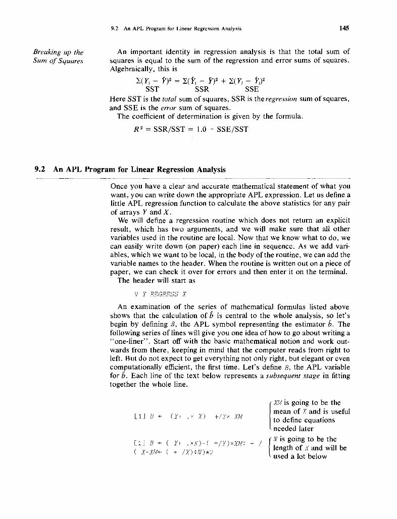
9.2 An APL Program for Linear Regression Analysis 145
Breaking up theSum of Squares
An important identity in regression analysis is that the total sum ofsquares is equal to the sum of the regression and error sums of squares.Algebraically, this is
~(Yi - Y)2 = ~(Yi - y)2 + ~(Yi - Yi)2SST SSR SSE
Here SST is the total sum of squares, SSR is the regression sum of squares,and SSE is the error sum of squares.
The coefficient of determination is given by the formula.
R 2 = SSR/SST = 1.0 - SSE/SST
9.2 An APL Program for Linear Regression Analysis
Once you have a clear and accurate mathematical statement of what youwant, you can write down the appropriate APL expression. Let us define alittle APL regression function to calculate the above statistics for any pairof arrays Y and X.
We will define a regression routine which does not return an explicitresult, which has two arguments, and we will make sure that all othervariables used in the routine are local. Now that we know what to do, wecan easily write down (on paper) each line in sequence. As we add variables, which we want to be local, in the body of the routine, we can add thevariable names to the header. When the routine is written out on a piece ofpaper, we can check it over for errors and then enter it on the terminal.
The header will start as
\j Y REGRESS X
An examination of the series of mathematical formulas listed aboveshows that the calculation of b is central to the whole analysis, so let'sbegin by defining B, the APL symbol representing the estimator b. Thefollowing series of lines will give you one idea of how to go about writing a"one-liner". Start off with the basic mathematical notion and work outwards from there, keeping in mind that the computer reads from right toleft. But do not expect to get everything not only right, but elegant or evencomputationally efficient, the first time. Let's define B, the APL variablefor b. Each line of the text below represents a subsequent stage in fittingtogether the whole line.
[lJ B +-
[1J B +
( X-XM+
(Y+ aX X) -t/Yx XM
y+ .XX)-( +/Y)xXM~
+ /X)~N)*2
[
XM is going to be themean of X and is usefulto define equationsneeded later
/ (N is going to be the+ length of X and will be
used a lot below

146 Elementary Linear Regression, Goodness of Fit, and Analysis of Variance (ANOV,A) Problems
(
XSQ is the sum of[lJ B+( ( Y + .xX)- ( +/Y)xXM)f squared deviations of(XSQ +- + / ( X-XM+ ( +/X)~N+p X)*2) x from XM, which will
also be used repeatedly
Reread line [1] from right to left, ensuring that it does what is intended andthat the parentheses match.
[2J A+ + /YfN-B xXM
[2J A+ « +/Y)~N)-BxXM
{+/Y~N is inefficient; Y~N-Bx XMdoes not work as intended
{This is nearly right, but we willneed the mean of Y later
Regression Routine
~2J A+- ( YM+- ( +/Y)+N)-BxXM
Check this line, which now seems reasonable, and let's proceed to thenext. The remaining lines will give you no problems. In the preface wecomputed these coefficients using .YffiX and we could have used that methodhere too. X would be an N-by-2 array where the first column is composedof Is. This method is presented in Chapter 13.
The whole program might look like this:
) CLEAR
CLEAR WS
\j Y REGRESS X
[lJ B+-« Y + .xX)-( +/Y)xXM)~ (XSQ~ +/ (X-XM+( +/X)~N~p X)*2)
[2J A+ ( YM+- ( +/Y)~N)- BxXM
[3J SST+- ( +/ (Y-YM)*2)
[4J SSE++ / ( y- ( A+BxX))*2
[SJ V+SSE~ ( N-2)
[6 J VB+V~XSQ
[7J VA+ (( XM*2)~XSQ)+~N)xV
[8J COV+-XMxV~XSQ
[9J RSQ+1-SSE+SST
[10J 'SAMPLE SIZE IS ' ;N
[11J 'MEAN OF X IS ' ;XM
f12] 'MEAN OF Y IS ' ;YM
[13J 'VARIANCE OF X IS ' ;XSQ~N
r14J 'VARIANCE OF Y IS ' ;SST~N
[15J 'VARIANCE OF ERROR IS ' ; V

9.2 An APL Program for Linear Regression Analysis
[16J 'COEFFICIENT OF A = , ;A
[17J 'VARIANCE OF A = , ; VA
[18J 'T-RATIO = ';A+VA*O.5
[19] 'COEFFICIENT OF B = , ;B
[20J 'VARIANCE OF B = '; VB
[21J 'T-RATIO = , ;B+ VB*O • 5
[22J 'COEFFICIENT OF DETERMINATION IS ' ;RSQ
[23J ' COVARIANCE ( A, B ) IS ' ;COV
Y~55 70 90 100 90 105 80 110 125 115 130 130
X~100 90 80 70 70 70 70 65 60 60 55 50
147
Sample Results ofRegression Routine
Y REGRESS X
SAMPLE SIZE IS
MEAN OF X IS
12
70
MEAN OF Y IS 100
VARIANCE OF X IS 187 .5
VARIANCE OF Y IS 525
VARIANCE OF ERROR IS 69.889
COEFFI-CIENT OF A = 210.44
VARIANCE OF' A = 158.03
T-RATIO = 16.74
COEFFICIENT OF B = 1.5778
VARIANCE OP B = 0.031062
T-RATIO = 8.95
COEFFICIENT OF DETERMINATION IS 0.88907
COVARIANCE (A. B ) IS -2.1743
Now you know how to calculate: various statistics used .in simple linearregression.
We can define Y = a+ bX, the residuals fJ = Y - Y, plot relationshipsbetween them, calculate the variance of the estimator Y, and so on. Just forpractice, try the routine RES/D, which will calculate the residuals and Yready for plotting or otherwise analyzing the results. Consider
VRESIDCOJv

148
Residual Routine
Elementary Linear Regression, Goodness of Fit, and Analysis of Variance (ANOVA) Problems
\} RESID
[lJ YH+A+BxX
[2J RES+Y-YH
[ 3 ] ' RESIDUALS'
[4J RES
[5J 'COMPUTED VALUES OF Y»») >Y-HAT'
[6J YH
RESID
RESIDUALS
2.333333333 1.555555556 5.777777778 0 10 5 20 2.111111111
9.222222222 0.7777777778 6.333333333 1.555555556
COMPUTED VALUES OF Y» ) ) ) >Y-HAT
52.66666667 68.44444444 84.22222222 100 100 100 100 107.8888889
115.7777778 115.7777778 123.6666667 131.5555556
9.3 Goodness of Fit, Contingency Tables, and ANOVA Problems
Chi-Square andGoodness o.f Fit
Chi-Square Distribution and Goodness of Fit
A number of statistical analyses of data are linked by their commonreliance on the chi-square distribution. The chi-square distribution is thedistribution of the random variable 1': defined by Y == L{Vr, where the Viare independent random variables, each distributed as a standardized normal. That is, it has a mean of zero and a variance of one. Stated symbolically, Vi is distributed as N(O, 1). The chi-square distribution depends onlyupon its degrees of freedom; in the above example, the distribution of Y ischi-square with N degrees of freedom.
One of the first uses of the chi-square distribution you will encounter inyour statistical travels is the "goodness of fit" test. In the goodness of fittest you are asked to decide whether an observed set of relative frequencies is consistent with some theoretical predictions. So suppose that youhave the traditional k cells; there are a total ofN observations, n 1 of whichare in the first cell, n2 in the second, and so on. n1 + n2 + · · · + nk = N.You assume that someone (maybe your favorite uncle) has given you thetheoretical probabilities Pi of getting an observation in each of the cells.Thus PI is the probability for the first cell, P 2 is the probability for thesecond, and so on, so that the expected number of entries in each cell isNP 1, NP z, . .. ,NPk. Your task is to compare the ni with the NP i, i = 1,

9.3 Goodness of Fit, Contingency Tables, and ANOVA Problems 149
Chi-SquareDistribution
2, . . . ,k, and the statistic you calculate is written mathematically as
W = I~ (n j~;Pj)2)
where W is distributed as a chi-square variable with (k - 1) degrees offreedom.
The APL expression is obtained in a straightforward manner. Our inputsto our chi-square function are two arrays, one for the ni and one for the Pi'i == 1, 2, ... , k. So let's begin by entering them:
N~15 7 4 11 6 17
PI+-6 p -;.6
We have here an experiment to test whether a die is unbiased. On theassumption that the die is unbiased, Pi = 1/6, i = 1,2, ... , k. This is a verysimple function, so we can build up our expression from the middle (rather,from the most important part of the expression) as follows. Using paperand pencil, we put down
First Stage: N-PIxN!l~+ IN
Second Stage: ((N-PIxNN~+IN)*2)-;'NNxPI
This will not do, since NN (reading from the right) has not been definedearly enough.
Third Stage: +/( (N-PIx NN)*2) t PIxNN+ -tIN
Goodness ofFit Routine
ContingencyTables
A suitable goodness of fit routine would look something like the following:
"V N GOODFIT PI
[lJ G+-+/ ((N-PIxNN)*2)-;.PIxNN+-+/N
[2 J 'CHI -SQ GOODNESS OF FIT STATISTIC IS ' ;G
[ 3] 'WITH '; (pN) -1; , DEGREES OF FREEDOM'
[4J V
Let's try our function. Enter it into the computer, and then call it by
N GOODFIT PI
CHI-SQ GOODNESS OF FIT STATISTIC IS 13.6
WITH 5 DEGREES OF FREEDOM
Contingency Tables
Now we can move on to something a little more ambitious that introduces some new APL concepts. Contingency tables are generated in thefollowing manner. Suppose that someone takes a sample of people, or

150
Two-WayClassification
Elementary Linear Regression, Goodness of Fit, and Analysis of Variance (ANOVA) Problems
machines, or whatever, and then classifies everyone or everything into twocategories. For example, people can be classified according to blood typeand color of eyes, machines by frequency of breakdown (i.e., once amonth, twice, three or more times) and number of defective items produced, and so on. The two-way classification produces a table of cells suchas that shown in Table 9.1.
Table 9.1. Two-Way Classification Scheme
Color of Eyes
BloodType
ABo
BI Br Gr G
In this example there are 12 (3 x 4) cells altogether. The entry in eachcell is the number of people in the sample who have the designated pair ofclassification characteristics. For example, the entry in the B row and Brcolumn would be the number of people in the sample with blood type Band eye color brown. Everyone in the sample has to be in one (and onlyone) of the cells, so if we add up all the cell entries we get the number ofpeople in the sample.* Let ni.b i = 1,2, ... ,r,j = 1,2, ... ,c denotethe number ofpeopJe in the cell (iJ) , wherer andc are the number of rowsand columns, respectively, in the table. The hypothesis to be tested with acontingency table is that the observed entries in any row (or coluInn) differfrom the expected nUlnber in the row (or column) only bv sampling variation. The expected number in the cell (iJ) is given by (ni.n,j)/N, where ni.is the ith row sum and n.j is thejth column sum, and N is the total numberof people in the sample (see Table 9.2).
Table 9.2. Expected Number of Observations in the Two-Way ClassificationScheme of Table 9.1.
Color of Eyes
BI Br Gr G
BloodType
A nIl n l2 n l 3 n14 1B n21 n Z2 n 23 n 24 :
Io n31 n 32 n 33 n 34 I n3.------- --------- -------------------------------------------------~-------n. l n.2 n.3 n A I N
I
The chi-square statistic for this problem is
W = I r "9 (nij - nj.njN)21=1 £..J=1 ni.n.j/N
which, if the assumption is true, is distributed as a chi-square distributionwith (r - 1) x (c - 1) degrees of freedom.* Our appologies to those with blood group AB or hazel eyes, We simply wanted to keep the sizeof the table down.

9.3 Goodness of Fit, Contingency Tables, and ANOVA Problems
Dyadic p: Reshape
151
Reshape p
Plus Reduction ofRows and Columns
Our first problem in handling this situation is how to enter a table like theone above into the computer. This reintroduces the dyadic use of p, calledthe "reshape" function. Consider the following examples:
A+-2 3 p 1 2
A
1 2 1
2 1 2
B+-2 2 pi 2 3 4
B
1 2
3 4
C+-2 2 p 1 2 345 6
C
1 2
3 4
The use of reshape rearranges the array given on the right-hand side intothe shape denoted by the left-hand side. If D is an array, then E+-M N p Dwill take the first n elements ofD and put them down as the first row of E,then the second n elements ofD become the second row ofE, and so on, mtimes. If there are too few elements in D, as shown in the example withA, then the elements of D are reused from the beginning until a table ofappropriate size is created. In APL such tables are known as two-dimensional arrays or tables, as opposed to the one-dimensional arrays or listswe have been having fun with so far.
Our first task is to obtain the row and column sums. With a one-dimensional array we know how to do this: +/(plus reduction). But with rows andcolumns, what happens? Try
+/A
4 5
So +/ on a two-dimensional array gives us plus reduction of the rows ofA .We get plus reduction of columns by a simple device. Try overstriking thereduction sign with the subtract sign; thus:
+IA
333
gives us plus reduction down columns.

152
Outer Product o. x
Elementary Linear Regression, Goodness of Fit, and Analysis of Variance (ANOVA) Problems
Outer Product
Now that we see how to get row and column sums, the next step is tocreate the table of entries: (ni.n.i)/N. This is most easily accomplished bymeans of what in APL is called the outer product. Suppose that x and yareany two single-dimensional arrays, say m and n in dimension, respectively,and we want the table created' by multiplying each element of x by eachelement ofy. Ifx has elements Xl' x2 , ••• ,Xm andy has elements YI, Y2' . .. ,Yn, then we want the (m x n) table of entries given by X1Yl, XIY2, XIY3,. • • ,
XmYn arranged into an (m x n) table. This sounds like a very complicatedarrangement, but once again what looks difficult is easy in APL. The (m x n)table we want is obtained by using the "'outer product," or jot dot product,which is o. x and is keyed by upper case J (gives the jot), period (gives thedot), and the multiply key. Thus we have
T+-Xo . XY
and T is the desired (m x n) table of entries. Let's try it. Recall theX and Ythat we have used before. In case you logged-off since last using them, wehave
X+-1 2 3 4 5 6 7
Y+-2 4 6 8 4 2 6
T+-Xo. xY
T
2 4 6 8 4 2 6
4 8 12 16 8 4 12
-6 12 18 24 12 6 18
8 16 24 32 16 8 24
10 20 30 40 20 10 30
12 24 36-
48 24 12 36
14 28 42 56 28 14 42
If you examine the entries of T you will see that the entry in the (i, J)position is the product of the ith element of X and thejth element of Y:
Now we can create a table of entries where the (i,j) entry in the table is(ni.n.i)/N. Let TB be the two-dimensional array of numbers nij. Write downour first attempt at creating the table:
R+-+/TB
C+-+ITB
Line [1] gives the row sums and line [2] the column sums. The third lineobtains N by adding up row sums, and divides that into the array of column

9.3 Goodness of Fit, Contingency Tables, and ANOVA Problems 153
totals which, in turn, is multiplied element by element by the elements ofthe array R. The new array is then subtracted from the original array TB,element by element, and the result is stored in TB again to save space (thestoring of a number of big tables soon uses up all of your available workspace). The new contents of TB contain elements such as (nij-ni.n.JIN).
The elements of the new array TB have to be squared and divided by theelements of (Ro. x( fN++IR). Let's try again.
NT-+-Ro . xCfN+-t IR
+1+/((TB+TB-NT)*2)--'NT
To be sure that you are following all this step by step, let's actually perform these operations with TB.
TB+2 3 02 3 1 1 4 2
R-+-+ITB
R
6 7
C+-+fTB
c
373
NT-+-Ro .. xCfN+ +IR
NT
1.384615358
1.615384615
3.230769231
3.769230769
1.384615385
1.615384615
Chi-SquareContingency TableRoutine
A routine for calculating the statistic of a contingency table might looklike the following:
V CONTAB TB;R;C;NT;W
[1J R++ITB
[2J C-+-+fTB
[3J DF+-(pTB)-l
[4J NT+Ro.xCfN++IR
[5.J W+-+I+ I (( TB-NT)*2) fNT
[6J 'THE CHI-SO STATISTIC FOR A'
[7J 'CONTINGENCY TABLE IS ';W
[8J 'WITH' ;DF[1]xDF[2Ji' DEGREES OF FREEDOM'
[9J V
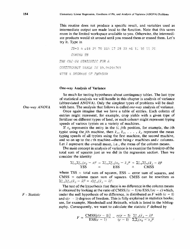
154
One-way ANOVA
F - Statistic
Elementary Linear Regression, Goodness of Fit, and Analysis of Variance (ANOVA) Problems
This routine does not produce a specific result, and variables used asintermediate output are made local to the function. Note that this savesroom in the limited workspace available to you. Otherwise, the intermediate products would sit around until you reused them or erased them. Let'stry it. Type in
TB~3 4 018 29 70 115 17 28 30 41 11 10 11 20
CONTAB TB
THE CHI-SO STATISTIC FOR A
CONTINGENCY TABLE IS 19.94264769
WITH 6 DEGREES OF FREEDOM
One-way Analysis of Variance
So much for testing hypotheses about contingency tables. The last typeof statistical analysis we will handle in this chapter is analysis of variance(abbreviated ANOVA). Only the simplest types of problems will be dealtwith here. The analysis that follows is called one-way analysis of variance.
Once again imagine that we have a table of entries. Each column ofentries might represent, for example, crop yields with a given type offertilizer on different types of land, or each column might represent typingspeeds of various typists on a variety of machines.
If Xu represents the entry in the (i, j)th position, for example, the ithtypist using thejth machine, then X,I' i,2' ... ,i.e represent the meantyping speeds of all typists using the first machine, the second machine,and so on up to the c th machine-there being c machines and c colulnns.Let i represent the overall mean, i.e., the mean of the column means.
The main concept in analysis of variance is to examine the breakup of thetotal sum of squares just as we did in the regression section. Thus weconsider the identity
,,"r ,,"c ( _ -)2 _ "r ,,"C ( _ -)2 ,,"r ""e (- -)2L.ii=IL.ij=l Xu X - L.ii=IL.ij=l Xu X.j + L.ii=lL.ij=l X.j - x
TSS ESS + CMSS
where TSS =: total sum of squares, ESS == error sum of squares, andCMSS == column mean sum of squares. CMSS can be rewritten as,,"r ~c (- -·)9 - ~e (- -)')L.ii=1 L.if=l X'.j - x ... - rL.ij =1 ~t,j - X -.
The test of the hypothesis that there is no difference in the column meansis obtained by looking at the ratio ofCMSS/(c - 1) to ESS/(rc - c) which,under the null hypothesis of no difference, is distributed as F with (c - 1)and c(r - 1) degrees offreedom. This is fully explained in statistics books;see, for example, Mendenhall and Reimuth, which is listed in the bibliography. Consequently, we want to calculate the statistic F defined by
F == CMSS[c(r - I)JESS(c - 1)

9.3 Goodness of Fit, Contingency Tables, and ANOVA Problems 155
Index of an Arrayof Dimensions
One-way ANOVAANOVAI
Let us suppose we have a table X ofe columns ofr entries each, and wewant to do a one-way analysis of variance on X by columns. From themathematical expression above we need column sums and the overall sum;but this is now very easy! Write down the following first attempt:
MCOL+-( +IX)~R+( p X) [1J
M+-( +/MCOL)~C+( p X) [2J
NUM+-RxCx( R-l)x+/C MCOL-M)*2
DEN+-( C-l)x+/+/ ( X- (R,C) pMCOL)*2
F+-NUM~DEN
The only new element here is (p X) [ 1 ] and (pX) [2 J. The expansion(pX) is an array of the dimensions ofX, so that (pX) [2J gives the second.If the parentheses had been left off, any attempt to execute pX[l] wouldhave given an error; thus
p X [lJ
RANK ERROR
p X [1JA
The reason for this is that once X has shape r xc, the expression X[ 1J isinvalid. What is needed to index a two-dimensional array is a pair ofindexing numbers, e.g., X[1;2J. More of this later. What we wanted, ofcourse, was the first element of the one-dimensional array (pX) .
You should also recall that to obtain an (R x C) table from MeOL, anarray ofC elements, we must write (R~C) pMCOL and not just R4C pMCOL,which produces a SYNTAX ERROR. This is because the pair of variables R Cis
not an array even though 8 3 would be. To produce an array with a set ofvariables it is necessary to catenate them; thus, (R, C) is an array of twoelements, Rand C.
An example of an analysis of variance routine for this simple problem is
V ANOVA1 X
[1J MCOL+(+tX)fR+(p X)[1]
[2J ~(+/MCOL)fC+(p X)[2]
[3J NU1~RxCx (R-1)x+/ (MCOL-M)*2
[4J DEN+ (C-1)x+/+/(X-(R,C) p MCOL)*2
[5] F+-NUM~DEN
[6] r THE F STATISTIC FOR ANALYSIS OF r
[7J 'VARIANCE ACROSS COLUl-1NS IS ';F
[8J 'WITH '; (C-1), 'AND ';Cx(R-1);' DEG FREEDOJ.1 '
[9J V

156
Two-way ANOVA
Elementary Linear Regression, Goodness of Fit, and Analysis of Variance (ANOVA) Problems
Now that we have it, let's try it. Type
TAB~8 3p 44 40 54 39 37 50 33 28 40,0
0:
56 53 55 43 38 45 56 51 66 47 45 49,0
0:
58 60 65
ANOVA1 TAB
THE F STATISTIC FOR ANALYSIS OF
VARIANCE ACROSS COLUMNS IS 1.868644068
WITH 2 AND 21 DEC FREEDOM
Two-way Analysis of Variance
The last problem that we will consider in this section is two-way analysisof variance. As before, we have a table of entries with r rows and ccolumns. With one-way analysis of variance we calculated only columnmeans; in two-way analysis we calculate both column and row means. Asbefore, the analysis of the test of the null hypothesis of "no effects" isbased on the breakup of the total sum of squares. Consider the identity:
~r=l~Y=l(Xij - X)2 = ~r=l~Y=l(Xij - X,J - X.i + X)2 + ~r=l~Y=l(X;. - X)2TSS = ESS + RMSS
+ CMSS
X is the overall mean, Xi, is the mean of the ith row, and x,J is the mean ofthejth column. RMSS is the row mean sum of squares and CMSS is thecolumn mean sum of squares. CMSS can be rewritten (as before) asr~f=I(Xj - X)2 and RMSS as C~r=I(.Xi. - X)2.
With these statistics we can test three different hypotheses:
HI: Row means are equal, column means are unspecified.H2 : Column means are equal, row means are unspecified.H3 : Rowand column means are both equal (not necessarily to each
other).
Hypothesis Hi is tested by the statistic F; defined mathematically by:
RMSS/(r - 1)F l = -=E=S-=-S-"'/["'-(r--~1)....,...(c--~1)~]
CMSS/(c - 1)F2 = -=E=-=SS=-/~[(;--r"":"_-':'1'7)(c-----"--:"1'"')]

9.3 Goodness of Fit, Contingency Tables, and ANOVA Problems IS7
F - (RMSS + CMSS)/[(r - 1) + (c - 1)]3 - ESS/[(r - l)(c - 1)]
Under the null hypothesis of no row or column effects, F 1 is distributed asF with (r - 1) and (r - l)(c - 1) degrees of freedom, F 2 as F with (c - 1)and (r - 1)(c - 1) degrees of freedom, and F 3 as F with (r - 1) + (c - 1)and (r - 1)(e - 1) degrees of freedom.
All we have to do now is to program a routine for calculating the statistics required for a two-way analysis of variance. Let's modify ANOVAIand call it ANOVA2.
So far we have not paid much attention to trying to make our routinescomputationally efficient or compact in terms of size of workspace used.This is because we felt you had enough to do in learning statistics and thebasics of APL all at once. But, since ANOVA2 will be similar to ANOVAl,let's take the opportunity to do things a little more efficiently than before.To this end, let's expand and simplify algebraically each of the sums ofsquares listed above.
ESS' "'r ""'c [2 -2 + -2 :-.2 + ..,;;; (_ - _ - +-)• ~1=l~i=l Xi) + XI. X.j + A- "'-"-Ii XI. X.j X
- 2Xi.( - X.j + i) - 2i.~]
'" -2 -2 ['" -2 :-.2]= e~-x· - rex = c ~·X· - rA -I I. I I.
= r~.i2. - rex2 = r[~,r2. - ex2]J J ,oJ
From the above expressions we see that the major sums needed are ~~Xri>
~ixL ~~~j, and x2 • We might begin by putting together the various sums andparameters required to calculate the main results. Consider, for a table Xof entries
R+(p X)[1]
C+(p X)[2J
XR+-+/X
XC++IX
{Gives us the R, C valuesneeded in the calculations
{Gives the row and columnsums
As noted above, there are three possibleF values we can calculate, all ofwhich require ESS/[(r - 1)(e - 1)] in the denominator. Consider thefollowing possible form for ANOVA2:
ANOVA2 V ANOVA2 X;RM;CM
[1J R+(p X)[lJ
[2J c+(p X)[2J

9.3 Goodness of Fit, Contingency Tables, and ANOVA Problems 157
F - (RMSS + CMSS)/[(r - 1) + (c - 1)]3 - ESS/[(r - 1)(c - 1)]
Under the null hypothesis of no row or column effects, F 1 is distributed asF with (r - 1) and (r - l)(c - 1) degrees of freedom, F 2 as F with (c - 1)and (r - 1)(c - 1) degrees of freedom, and F 3 as F with (r - 1) + (c - 1)and (r - l)(c - 1) degrees of freedom.
All we have to do now is to program a routine for calculating the statistics required for a two-way analysis of variance. Let's modify ANOVAIand call it ANOVA2.
So far we have not paid much attention to trying to make our routinescomputationally efficient or compact in terms of size of workspace used.This is because we felt you had enough to do in learning statistics and thebasics of APL all at once. But, since ANOVA2 will be similar to ANOVA1,let's take the opportunity to do things a little more efficiently than before.To this end, let's expand and simplify algebraically each of the sums ofsquares listed above.
ESS· ~r ~c [2 -2 -2 ~ + 2- (- - - - -)• 4Ji=l4Jj=l Xii + Xi. + X.j + A,- Xij Xi. X.j + x
-2Xi.(-i. j + i) - 2i.~]
RMSS · ~r ~c [-2 -2 - 2- -]• ~i=l~j=l Xi. + X Xi-X
== cL·i~ - rcx2 == C[L'X~ - ri2]1 1. 1 1.
= r~·i2. - rci2 == r[L.y2, - ci2]J .J 'yo.-.J
From the above expressions we see that the major sums needed are ~~Xrj,
~iir., ~~~j, and i 2• We might begin by putting together the various sums and
parameters required to calculate the main results. Consider, for a table Xof entries
R+-(p X)[1]C+-( p X) [2 J
XR+-+/XXC+-+fX
{Gives us the R, C valuesneeded in the calculations
{Gives the row and columnsums
As noted above, there are three possibleF values we can calculate, all ofwhich require ESS/[(r - 1)(c - 1)] in the denominator. Consider thefollowing possible form for ANOVA2:
ANOVA2 \J ANOVA2 X;RM;CM
[ 1 ] R+- (p X) [ 1 ]
[2J C+-(p X)[2]

158 Elementary Linear Regression, Goodness of Fit, and Analysis of Variance (ANOVA) Problems
[ 3 J RM~-( +/ X) -;- C
[4J GM~( +/ ( CM~ ( +!X)-;-R»-;-C
[5 J RMSS~Cx ( (RRM++ / ( RM*2») -RxGM*2)
[6J CMSS+Rx( CCM+-+/CM*2)-CxGM*2
[7J ESS+(+/+/X*2)+( -CxRRM)+( -RxCCM»+CxRxGM*2
[8J DEN+ESS~DDF+« R-l)x( C-l»
[9J Fl~RMSS~DENx( R-1)
[10J F2+-CMSS+DENx( C-l)
[11J F3+( RMSS+CMSS)~DENx( R+C-2)
[12J 'THE F STATISTICS FOR TWO-WAY ANOVA ARE: '
[13J 'TESTING ROW MEANS, FIS ';Fl
[14J 'WITH '; ( R-1)!JDDF;' DEC. FREEDOM'
[15J 'TESTING COL. MEANS, F IS ';F2
[16J 'WITH '; CC-l),DDF;' DEG. FREEDOM'
[17] 'TESTING ROW AND COL. MEAN~c;, F IS ' ;F3
[18J 'WITH '; ( R+C-2),DDF;' DEC. FREEDOM'
[19J \J
There are a few points in this routine worth noting. First, the numberof operations performed has been reduced. This was made possible byshowing that the required algebraic expressions depended upon a smallnumber of partial sums. Second, intermediate results are stored in avariable for use later in the rOlltine (see, for example, lines [4], [5], and [6]).Third, an attempt was made to ensure that where a sum of variables isdivided (or multiplied) by the same constant, the sum is taken first, thenthe result is divided (or multiplied). In general, it is better to multiplybefore dividing in a complicated expression since this reduces the propagation of errors introduced by the process of division. This rule was notfollowed entirely in this routine since it was, in fact, more efficient to formthe denominator first, because it was used repeatedly.
Line [7] is interesting in that it poses a trap for those who forgetthat the computer operates from right to left. If we had writtenESS++ /+ / X*2-CxRRM-RxCCM+CxRxGM, we would have obtained an erroneous result. CxRxGM is alright, but then this is added to CCM, which sum isthen multiplied byR, leading to the first error. The result (ofRxCCMxCxRxGM)is subtracted fromRRM, leading to the second error, and so on. Note thatthe minus operator signs used with Rand C are being used in their monadicsense; -C and -R change the signs of C and R.

9.4 *Calculating the Chi-Square and F Distributions
TAB
44 40 54
159
Results fromANOVA2
39 37 50
33 28 40
56 53 55
43 38 45
56 51 66
47 45 49
58 60 65
ANOVA2 TAB
THE F STATISTICS FOR TWO-WAY ANOVA ARE:
TESTING ROW MEANS, F IS 29.46666667
WITH 7 14 DEC. FREEDOM
TESTING COL. MEANS, F IS 19. 6
WITH 2 14 DEC. FREEDOM
TESTING ROW AND COL. MEANS, F IS 27.27407407
WITH 9 14 DEC. FREEDOM
While this routine is neither as compact nor as elegant as it might be, ithas served the purpose of demonstrating some of the factors you should bebeginning to take into consideration. The major ones are:
1. Keep the use of big arrays, especially tables, to a minimum-they useup an incredible amount of workspace.
2. Simplify the algebra as much as possible before beginning to write theroutine.
3. Avoid repeating calculations.
9.4 * Calculating the Chi-Square and F Distributions
In this short section we will discuss how to calculate the chi-square and Fprobability distributions so that you need not use the tables and can pickconfidence levels and sizes of tests not available there. More importantly,by plotting the distributions you can acquire a better understanding ofthem than would otherwise be the case.
Let's begin with the chi-square distribution. If Y is distributed as chisquare with N degrees of freedom, its density can be written as:
_ YN/2-l> Exp (- Y/2)F( YIN) - r(N/2) 2(N/21
(See, for example, Press in the bibliography.)

160
r Gamma Function!X
Elementary Linear Regression, Goodness of Fit, and Analysis of Variance (ANOVA) Problems
The non-APL symbol f(N /2) represents the gamma function, whichgeneralizes the factorial. If N /2 is an integer, then r(N/2) = (N/2 - 1)!.f(p) is defined by the integral
fcp) = Jooo xP-1e-·rdx
Ifp is an integer, r(p) = (p - 1)!. The chi-square distribution of Y withN /2 degrees of freedom is nothing more than the gamma distribution of thevariable Y/2 with parameter p = N /2. In APL, f(N/2) is easily calculated;in fact, f(N/2) is given by !(N -;- 2) - 1, even where N -7- 2 is a noninteger.
In order to calculate the integral of F(ytN) from zero to some bound B,we will have to use a numerical approximation. The simplest procedure to follow is that used in obtaining the Normal integral whereby webroke the interval over which the function is to be integrated into a seriesof small intervals and added up the approximate areas to get the integral.Before continuing you might wish to review briefly section 6.3 in Chapter 6.
How many intervals are needed? Or rather, how small should eachinterval be? If we regard the interval from 0 to 10V2N, where \I2N is thestandard deviation, as the effective range of the variable 1': Le., integrationof the density function over this range gives a value close to one, and if weregard a ·suitable interval length as a 32nd of a standard deviation, then integration over the effective range would involve 320 intervals. For an integration from 0 to B, we need to determine how many intervals are needed.Note that we do not want to divide the interval 0 toB by some fixed numbersince the accuracy of the integral would vary tremendously with variationsin the value ofB. Figure 9.1 will help clarify our stratagem. In the sampleshown, the interval zero to B should be broken up into 9 sub-intervals.
Figure 9.1 Illustration of a Method for Determining Integration Intervals
Intervals for Range (0, 10 V2N)
1llllllllllllllllmllll,1o
--B
--10 V2N
1-1-'-1-1-'-1-1-1-1o BI Represents interval boundaries• Represents interval mid points
Thus, the required number of sub-intervals can be obtained in APL asfollows:
L+ (O,t320)x((2xN)*O.5)f32
NINT+t /B>L
The first line produces 321 points on the interval from 0 to 10 V2N and thesecond line gives, by compression, the numbers of such points less than Band hence the number of intervals into which 0 to B is to be divided.

9.4 *Calculating the Chi-Square and F Distributions 161
The idea underlying the approximation of the integral is uncomplicated. * On each sub-interval, we will approximate the actual area underF( Y~N) by a rectangle whose base is given by BW (B - 0) -;- NINT andwhose height is F( y* IN), where y* is the mid-point of the interval. Thisapproximating procedure is known as the rectangular method. It is thesame as that used in Chapter 6 to calculate the cumulative normal distribution. A brief glance at figure 6.2b will remind you of the main idea.
The sequence of mid-points at which F( YlN) is to be calculated is given by
YS~((lNINT)xBW)-BW~2
In Figure 9.1 above, these points are shown as the dots on the interval[0, B].
We now have most of the pieces, so that all we have to do is fit themtogether. Consider
CumulativeChi-Square
'J W~N CUMCHISQ B;YS
[1J DEN~(2*NN)x!(NN~N~2)-1
[2J NINT~+/B > L~(O,1320)
x«(2 xN)*O.5)f32
~N = degrees of freedomB = boundary of integration
+-Calculates denominatorof F(Y~N)
~{Determinesnumber ofintervals needed
[3J YS~( ( lNINT)xBW)-(BW~B~NINT)-;-2 ~Midpoints of the intervals
[4J FYS+( YS*(NN-1) }x*( -YS-i-2) ~Evaluates the density at YS
[5J W+(W++/PYSxBW)~DEN
[6J 'THE CUM CHI SQ DISTN ,
[7J 'WITH' ;N;' DEC FREEDOM'
[8J 'F(B) IS ';W
[9J '1-F(B) IS ';(1-W)
[10J 'J
+-[ W gives probability ofrandom variable distributedas F( YJN) of being lessthanB.
Let's try our function and compare its results with those obtained fromthe Biometrika Tables prepared by Pearson and Hartley. The official tablesgive the following numbers.
Comparison of Biometrika Table Chi-Sq Values
APL-STAT Resultsn.F\ B 0.1 1.0 5.0 10.0
and TabulatedValues 1 0.24817 0.68269 0.97465 0.99943
2 0.04877 0.39347 0.91791 0.993265 0.00016 0.03743 0.58412 0.92476
10 0.00017 0.10882 0.5595120 0.00028 0.03183
* Any advanced calculus text or book on numerical approximation will discuss various methods. Oneuseful reference is W. Kaplan, Advanced Calculus, Addison-Wesley, 1952, Reading, Mass.

162
Cumulative FDistribution Routine
Elementary Linear Regression, Goodness of Fit, and Analysis of Variance (ANOVA) Problems
Approximate APL Chi-Sq Values
D.F\ B0.1 1.0 5.0 10.0
1 .20434 .63228 .92400 .947672 ,04877 .39345 ,91788 .993225 .00016 .03741 ,58414 .92478
10 .00017 .10881 .5595120 ,00028 .03182
There are a few items worth mentioning with this routine. First of all, inthe header to the function, the name was given as CUMCHISQ, instead ofsomething like CUMCHI~SQ. The reason for this is that a symbol such as,, - " cannot be used in the definition of a function name. Further, and veryimportantly, the way in which the function is written, the arguments NandB must be scalars, not arrays. If you define either N or B as an array andattempt to use CUMCHISQ, you will get the response
LENGTH ERROR
CUMCHISQ[1] NINT++/B > L+(O,320)x(2 xN)*O.5)+32
if N is an array, or the caret will be under B, if only B is an array.However, the most important lesson from the above tables is that while
the routine provides a useful approximation to the correct values for degrees of freedom greater than 1, the approximation is very bad for onedegree of freedom, and we shall not bother with this now. However, youshould note that the difficulty is not simply one in which the interval widthis too broad. If you were to examine a plot of the densities for 1, 2, 3, and 4degrees of freedom, you would see considerable differences in the shapeof the chi-square distribution as the degrees of freedom increase in thisrange as shown in the graph in problem 10. What is required is a much moreaccurate approximating procedure-our simple rectangular procedure isinadequate for the task; some suggestions are contained in the exercises.
Let us consider the F distribution with k 1 and k 2 degrees of freedom. The. density function can be written as:
,
ji(w) = (kdk2)kl
/2r«k1 + k2)/2) W(k, /2l-J( 1 + (k /k) )-<k l +k2 )/2
fk1/2)r(k2 /2) 1 2 w
The terms involved in the constant of integration present no difficulty afterthe chi-square distribution. Since our strategy for obtaining the cumulative distribution worked reasonably well with the chi-square distribution,let's try it with the F distribution, whose standard deviation in algebraicterms is:
2k~(kl + k2 - 2)k t (k2 - 2)2(k2 - 4)
where k must be greater than 4 for the variance to be defined.The F cumulative distribution function routine can be set up in a manner
very similar to that of the chi-square distribution. The main differences

9.4 *Calculating the Chi-Square and F Distributions 163
Comment f1
occur in the fact that the F distribution has two degrees of freedom insteadof one and ""FYS" has a different definition in the two routines. Try thefollowing:
\J W+-P CUMF B
[1J RTHIS ROUTINE CANNOT BE USED WITH
[2 ] ~LESS THAN FIVE DENOM, DEC. OF FREEDOM.
[3J CONST+-(!«PS++/P)+2)-1)xP[lJ*Pl+-P[lJ+2
[4J CONST+-CONST~(!(P[2J+2)-1)x(!Pl-1)XP[2]*Pl
[5J ST~2x(PS-2)xP[2J*2
[6J STD+-(STD+(P[1]x(P[2]-4)x(P[2]-2)*2))*0.5
[7J NINT++/B > L~(O,1320)xSTD+32
[8J YS+« lNINT)xBW)-(BW+B+NINT)+2
~g] FYS+-(YS*P1-1)x(1+(P[1]+P[2])XYS)*( -PS+2)
[10J W+-(W++/FYSxBW)xCONST
[llJ 'THE CUMULATIVE F DISTN WITH'
[12J P[l];' AND ';P[2J;' DEC. FREEDOM'
[13J 'IS ';W
[14J V
The first two lines of this routine form a comment which will warn theuser when he displays the function that it cannot be used with less than fivedenominator degrees of freedom. The comment symbol is made by keyinguppershift C(called cap), backspace, and uppershift J (or jot). Everythingto the right of this symbol is regarded as a comment. When the function isexecuted, comments are ignored; they are only printed when the function isdispLayed.
B is one limit of integration; 0 is assumed to be the other, in that we arecalculating the probability of the random variable being contained in theinterval [0, B]. The array P contains the degrees of freedom, k v k 2.
In the calculati{)n of the integral of f(w) there are two component partsmultiplied together, a constant:
(k l / k2)kJ/2r«kl + k2)/2)f(k l / k2)r(k2 /2)
and that portion of the function to be integrated is
W(k l /2)-1( I + (kl
/ k2)w!(k1 +k2)/2
In calculating the integral the multiplicative constant can be calculatedseparately from the second part and the two multiplied together to get theanswer.

164
Example of Use ofCumulative FDistribution Routine
Elementary Linear Regression, Goodness of Fit, and Analysis of Variance (ANOVA) Problems
Lines [3] and [4] determine the value of the constant term; line [31produces the numerator and [4] the denominator. Remember that r(k t /2) isobtained in APL by !(P[lJ~2)-1 since algebraically, r(k1/2) == (k1/2 I)!, when k1/2 is an integer. The APL function "factorial", !, is really thegamma fllnction.
Lines [5] and [6] calculate the standard deviation of the distributionwhich is needed for determining the interval widths.
Lines [7] to [10] determine the probability of the random variable lying inthe interval [0, B] in a manner very similar to the previous effort.
As a check on the accuracy of the routine, examine the following table.The table shows the probabilities obtained from the routine using variouscombinations of degrees of freedom and bounds. At the head of eachcolumn the theoretically correct probability is listed.
Table of Probabilities from F Distributions*
SPrOb..75 .95 .99 .999D.F.
(1,5) 0.66 0.86 .90 0.91(1.69) (6.61) (16.26) (47.18)
(1,10) 0.69 0.89 0.93 .94(1.49) (4.96) (10.04) (21.04)
(2,5) 0.75 0.95 0.99 0.998(1.85) (5.79) (13.27) (37.12)
(4,5) 0.75 0.95 0.99 1.000(1.89) (5.09) (11.39) (31.09)
(4,10) 0.75 0.95 0.99 0.999(1.59) (3.48) (5.99) (11.28)
(10,20) 0.75 0.95 0.99 0.999(1.40) (2.35) (3.37) (5.08)
* The bound B is given in parentheses below the probability.
Once again, as with the chi-square distribution, we see that one degreeof freedom in the numerator causes difficulties with the approximation. Asboth degrees of freedom increase, the relative accuracy increases. This isbecause the functions being approximated are easier to handle with oursimple rectangular procedure. Greater accuracy and less computation canbe obtained with a more sophisticated procedure, such as the use ofSimpson's rule.
An example of use of the routine is:
p
1 5
B
1.69
P CUMF B
Summary
Summary
THE CUMULATIVE F DISTN WITH
1 AND 5 DEC. FREEDOM
IS 0.662880113
0.662880113
165
REGRESS: Simple least squares regression-an APL routinewas provided to calculate most of the relevant statistics in a simple linearregression model of the type Y = a + bX + u.
GOODFIT: a routine to perform goodness of fit tests.
CONTAB: a routine for calculating the statistics required in testsof hypotheses within a contingency table.
ANOVA1: a routine for carrying out simple one-way analysis ofvariance.
ANOVA2: a routine for performing two-way analysis of vari-ance.
Reshape, p (uppershift R): a dyadic function which rearrangesthe "array shape" of the right-hand argument as specified by the left-handarray. Example:
C+-2 3 pA
rearranges the elements of the array A into a table (matrix) composed oftwo rows of three columns each; elements fromA are stored in the variableC row by row in sequence from the elements of A.
Outer Product, o. x (jot dot) (uppershift J), period, multiplication): a dyadic function which multiplies each of the m elements in theleft-hand argument array with each of the n elements in the right-handargument array to form a table of dimension (m x n) containing all m x nmultiplications.
Reduction, /: a monadic function. When used over two-dimensional arrays (tables or matrices) IITABLE produces an array formed by theI reduction of each rol'V of TABLE, where f is one of the arithmeticfunctions.
Reduction, / by columns for a two-dimensional array is obtained byusing f (reduction, backspace, minus sign).
Gamma function, ! (uppershift K, backspace, period): a monadicfunction to evaluate the gamma function, which generalizes the factorialfunction. !P in APL produces the mathematical result of f(P + 1).
CUMCHISQ: a routine to calculate the integral of the chisquared density function.
CUMF: a routine to calculate the integral of the F density func-tion.

166 Elementary Linear Regression, Goodness of Fit, and Analysis of Variance (ANOYA) Problems
Comment, R (uppershift C, backspace, uppershift J) used as thefirst character of a line inside a function to provide explanatory commentswhen function is displayed. Comments are not printed on execution offunction and are otherwise ignored.
Exercises
APL Practice
(h) COY (A, B) = [2.:(X~~2 .W ] 5;,
1. For the two arrays X+120 and Y+-5+120, use your knowledge of APLto perform the following calculations based on the mathematical formulas listed below. These formulas are useful in regression analysis.
L{l(Xi - i)(Yi - y) estimator of the regres-(a) B = (x; - i)2 sion slope coefficient.
-~ == LXiinandY == "ZYi/n
(b) A == Y - B.¥: estimator of the constant term
(c) Ui = Yi - A - BXi' i = 1, 2, ... ,n vector of estimatederrorssum of the squares ofthe errorestimator of varianceof disturbance terms
estimator of the variance of the slope
estimator of the variance of the constantterm
estimator of the variance of the covarianceof the estimators AandB
(i) R = 2.:(x; - ·t')(Yi - .5')nSJ'Sy
where
simple correlationcoefficient of x and Y
S.r = ~(Xi - i)2/(n - 1), andSy == ~(Yi - y)2/(n - 1)
(j) SST = ~(Yi - y)2SSR = ((A + BXi) - y)2
total sum of squaresregression sum ofsquares
(k) RS = ~~~ a~d compare y?ur .answer with that in (j), the coeffiCIent of determInatIon.

Exercises
the variance of thepredicted value of ygiven Xo
167
t-statistic of the predicted value
(m) T = Y - (A + Bxo)
I( 2 [ 1 (xo - X)2 ])V Su 1 + Ii + I(Xi - i)2
2. This exercise introduces you to some novel ideas about constructingsome matrices that you will find useful in the following chapters. LetI~110.
(a) Io. =I produces the identity matrix
(b) a 3[ 1+I 0 • ~IJ produces an upper triangular matrix
(c) a 3[ 1+Io . =I] produces a diagonal matrix
(d) 2 3[1+(Io. =I)~1J a symmetric matrix
(e) 10 10 p'111 a circular matrix
(t) 10 10 p2 3,(8 pO),3 a tridiagonal matrix
(g) Va. =V where V+-1 1 1 2 2 2 2 3 3 3 3 3 , a block diagonalmatrix
3. The following exercises are basic to calculations inANOVA problems.For any matrix X nxk where n is the number of rows and k is the
number of columns, use your APL to write a routine to calculate eachof the following:
(a) Row means
(b) Column means
(c) Total mean and compare to (d) and (e)
(d) Mean of row means
(e) Mean of column means
(f) The mean of the squared differences of each element from the totalmean
(g) The mean of the squared differences of each element from its ownrow mean
(h) The mean of the squared differences of each element from its owncolumn mean
(i) The mean of the squared differences of each element from its ownrow maximum value
4. You might want to see where the total variation of any contingencytable might come from. Let the matrices A, B, C, D represent fourdifferent sets of tabulated data of ninety observations which you wishto analyze.
A == [~~ ~~ ~~]10 10 10
B == [1~ ~~ ~~]16 10 4

168 Elementary Linear Regression, Goodness of Fit, and Analysis of Variance (ANOVA) Problems
c=[~ 1~ ~i]8 13
D == [ ~15
1~ 1~]8 13
Use your program in Exercise 3 to get all the quantities given by theprogram for all four matrices. Comment on the results.
* 5. Let F(P) = Jooo xP~le~·rdx
Find F(20) and F(3.5) using the generalized APL factorial.
Statistical Applications
1. You are given the following data:
xy
65 63 67 64 64 68 62 70 66 68 67
68 66 68 65 69 66 68 65 71 67 68
69 71
70 65
where X is the height of the father and Y is the height of the son, bothmeasurements taken to the nearest inch. The objective is to find out ifthe height of the son depends on the father's height, and if so what isthe specific relationship between the fathers' and sons' heights. Useyour Y REGRESS X function (page 146) to find out which one of thefollowing regressions fits the data best.
(a) Y == a + bx + u
(b) Y == a + bx2 + U
(c) Y == a + b In x + u ~ eY == eUxbeu
(d) In Y == In a + x + u ~ Y == ae.TeU
(e) In Y == In a + b In x + u ¢::> Y = axbeu
(f) Y == a + (b/x) + u
Use as your criterion for best fit that regression which produces thehighest sample value for the coefficient of determination.
For each equation plot the residuals u == y - Yagainst Y. Commenton your observations.
2. Use the routine Y REGRESS X (page 146) to solve the following problem.
You are given the data:
xy
z
64
57
8
71
59
10
53
49
6
67
62
11
55
51
8
58
50
7
77
55
10
57 56
48- 52
9 10
51
42
6
40
30
2
68
57
9

Exercises 169
where X == weight to the nearest pound, Y == height to the nearestinch, and Z == age to the nearest year of 12 boys.
Run the following regressions in order to discover to what extentthe variables X, Y, and Z are linearly related.
at : X = a + by + UI
~ : Y = a + bx + U2
a3 : Y = a + bz + U3
a4 : X = a + bz + U4
After making the required transformations, run the regressionsas : loglo Y = a + b loglo X + Us
~ : Y = a + b/x + U6
a7 : Y = a + b log X + U7
as : Y =a + b log Z + Us
ag : Z = xbe1l9' which can be written as Z = In a +
b In x + Ug
Explain intuitively the meaning of each equation and of the estimatedas and bs.
3. The following data give the yields of wheat on some experimentalplots of ground corresponding to four different sulphur treatments forthe control of rust disease. The treatments consisted of:(1) dusting before rain(2) dusting after rain(3) dusting once each week(4) no dusting
Test to see if there are any significant differences in the yields due tothe dusting methods.
Dusting method
Plot 1 2 3 4
1 5.3 4.4 8.4 7.42 3.7 5.1 6.0 4.33 14.3 5.4 4.9 3.54 6.5 12.1 9.5 3.8
4. The number of units of work done per day by five workers using fourdifferent types of machines is given in the following table. Eachworker operated each type of machine for one day. Find estimates ofthe differential effects due to(a) machine type
(b) worker's skill
In each case, specify carefully the maintained, null, and alternatehypotheses

170 Elementary Linear Regression, Goodness of Fit, and Analysis of Variance (ANOVA) Problems
Units of Work Output by Type of Machine and Worker
Machine Type
Worker
12345
I II III IV
40 40 48 3640 42 50 4835 37 45 3242 36 48 3036 40 50 40
(c) Now suppose that you were not able to get the observation (3,III), i.e., the number of units for the third worker using the thirdmachine. How would you answer questions (a) and (b)?Some suggestions are:
1. Put some row or column average in the (3, III) position.2. Change the routine in such a way that you need use only three
observations for the third row and four observations for thethird column.
5. Put the cumulative F distribution function (page 163) into your workspace. Add some lines to ANOVAl and ANOVA2 functions alreadydefined in order to give the answers of hypotheses tests immediately,so that you don't have to look up the F tables.
6. Add some lines to the function Y REGRESS X to obtain the followingstatistics.
(a) the vector of calculated ~ call it Y(b) the vector of calculated residuals, call it 0 == y - y(c) the mean of X, ~ and Y(d) var (0) and var (n
7. Poultry researchers investigated the weight gains (in pounds) of fourtypes of "super" or "Industrial" turkeys fed three different rationsover a period of several months. The results are listed below:
Type of RationType ofTurkeys 2 3
A 50 45 35B 41 38 45C 61 35 55D 55 59 61
Find estimates of the differential effects of (a) rations, and (b)types, and test the hypotheses:
(a) Ho: The variations of weight gains is due to the different rations,regardless of the type of turkey.against HI: The rations have no effect on gains.

Exercises 171
(b) Ho: The variation of gains is due to the type of turkey, regardlessof the rations.against H 1 : The type of turkey does not affect gains.
(c) Ho: Neither the type nor the ration affects the weight against H 1 :
At least one of type or ration affects the weight.
8. The following diagram will help you understand the role of the degreesof freedom (n) of the X2 distribution. Let X2 represent the randomvariable andf(X2
) the corresponding density function.
fn(x2)n = 2
n = 10
B
Notice that for the same upper bound (B) and increasing degrees of
freedom the value of the integral,JoB f,b2)dx2, decreases in n.
(a) Use your N CUMCHISQ Bfunction (page 161) to verify this forN==1, 2, 3, . . . ,20 and B == 5.
(b) Use the N CUMCHISQ B function (page 161) to calculate theintegrals for N == 20 and B = 1,2,3,4,5,6,7,8,9, 10.
(c) Alternatively. How would you use the N CUMCHISQ B function todetermine the value of B for which the area from 0 to B is 87%when N = 20? Notice that the value of 87% is not in the tables ofthe chi-square distribution given by most textbooks.

10
Matrix Algebra in APLHow Simple It Is
10.1 Vectors, Matrices, and Arrays
Vectors, Matrices,and Arrays
Arrays, ColumnVector, Row Vector
172
Up to this point in our discussion we have dealt with variables which canbe scalars or which can be arrays; arrays have one or more dimensions,scalars are dimensionless. You will recall that if we define the variable V byV +-H some number," p V produces Hblank" because a scalar has no dimension, and PP V (which is the dimension of the number of dimensions)produces O. But if V is defined by V +- "a list of numbers," p V produces thenumber of elements in the list and pp V produces 1 (the number of elements in the list of dimensions).
Chapter 9 introduced a very important extension to our definition ofvariables-variables defined as two-dimensional arrays which can be visualized as a table of entries with rows and columns. In this chapter we willdevelop our APL tools for handling two-dimensional arrays and we willdistinguish between APL expressions such as "arrays" and mathematicalexpressions such as "vector" and' 'matrix. " In Chapter 11 we will extendthe examination of arrays in APL to three and higher dimensions!
Following the theme of this book, we will relate the APL expressionsdirectly to the mathematical operations you have learned, or are learning,in matrix algebra. Even if you do not know any matrix algebra at all, thisbook will help you to learn some.
A matrix is a two-dimensional array. Its dimensions, say (n, m) (sometimes this is written as (n x m), signify that the matrix has n rows and mcolumns. But what if either m or n is I? If the matrix is 1 x m (one row, mcolumns), it is called a row vector (or often just a vector for short). And ifthe matrix is n x 1 (n rows, 1 column), it is called a column vector (just avector for short). So you see that when referring to a vector, you have tobe careful to distinguish between row vectors and column vectors.
Now a row vector is not a column vector is not a list! (Remember, a listhas only one dimension: length.) "Array" in APL is a general term indicat-

10.1 Vectors, Matrices, and Arrays 173
Reshape p
ing a variable with one or more dimensions. An array with one dimension isa list; an array with two dimensions is a table. Mathematically, we need tobe a bit more precise, so we will often have to be careful to distinguish rowand column vectors from each other, from matrices, and especially fromlists.
If you have a list, say A, and you want to make it a vector, either columnor row, then use dyadic p. For example,
A+- 1 2 3 4
A is a list.
CV+-4 1 pA
CV is a column vector, or a matrix of dimensions (4, 1).
RV+-l 4 pA
RV is a row vector, or a matrix of dimensions (1, 4).Now type
A
1 2 3 4
CV
1
2
3
4
RV
1 2 3 4
A , CV, and RVare all arrays.
pA{4 elements in a list.
4
Ravel t
pCV
4 1
pRV
1 4
Now try:
B+,CV
pB
4
{4 rows, 1 column in a column vector.
{I row, 4 columns in a row vector.
{Ravel "," converts the column vector CV into a list.

174 Matrix Algebra in APL-How Simple It Is
pD
4
{
Again, the monadic function ravelconverts the row vector RV into alist.
So now you know that lists and vectors are different, how to get vectorsfrom lists (use reshape p), and how to get lists from vectors (use ravel, ).
10.2 Elementary Matrix Operations
Our first task is to define some matrices to use as examples. Try
A23+2 3 pi 2 3 456
A 13+-1 3p1 2 3
A31+3 lp3 2 1
A33+-3 3p1 2 3 3 214 2 3
B23+-2 3 p 1 2 3 456
B31+3 1p4 1 2
B13+1 304 1 2
Naming of matrices is arbitrary. You could have used DOG or MOUSE, etc.Our name choice was intended to make the dimensions easier to understand.
Now that we have defined a number of two-dimensional arrays, we willneed to consider how to refer to individual elements of an array. Consider
A33[1;2]
2
A23[2;3]
6
831[2;lJ
1
That's easy enough, but what if we want to refer to a whole row or columnofA33? How could we do that? Try
A33[1; ]
123
A23[ ;2J
2 5
Notice that with A3 3 [ 1; ] and, more strikingly, with A23 [ ; 2 ] the arrayreturned is a list, not a row or column vector. Thus
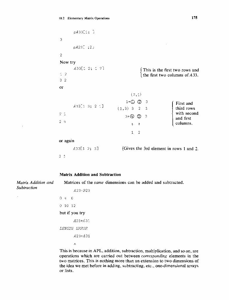
10.2 Elementary Matrix Operations
pA 3 3 [1; J
3
pA23 [ ; 2 ]
2
Now try
A33[1 2; 1 2J
1 2
3 2
or
175
{This is the first two rows andthe first two columns ofA 33.
( 2,1)
1+(D (6) 3 First andA33[1 3; 2 1J
( 1, 3) 3 2 1 third rows2 1
3-+@ ~with second
3 and first2 4 columns.t t
1 2
or again
A33[1 2; 3J
3 1
Matrix Addition and Subtraction
{Gives the 3rd element in rows 1 and 2.
Matrix Addition andSubtraction
Matrices of the same dimensions can be added and subtracted.
A23+B23
046
o 10 12
but if you try
A23+A31
LENGTH ERROR
A23+A31
/\
This is because in APL, addition, subtraction, multiplication, and so 00, areoperations which are carried out between corresponding elements in thetwo matrices. This is nothing more than an extension to two dimensions ofthe idea we met before in adding, subtracting, etc., one-dimensional arraysor lists.

176
MultipLy Matrix bya Scalar
MatrixMultiplication +. x
Matrix Algebra in APL-How Simple It Is
Multiplying a Matrix by a Scalar
Multiplying a matrix by a scalar is obviously easy:
3xA23
369
12 15 18
and forming linear combinations of vectors is also easy. Try the mathematical relation 2(A31) + 3(B31); in APL this is
(2 xA31)+3 xB31
18
7
8
What would happen if we removed the parentheses? Try it.
Matrix Multiplication
The mathematical operation of matrix multiplication (to be distinguishedfrom the APL operation of multiplication between arrays, e.g., A23 x B23)is nothing more than the APL function called inner product (defined onpage 27) between the rows of the first matrix and the columns of thesecond. The mathematical expression for the matrix multiplication of twomatrices B23, A33 to give a matrix C is C = (B23) (A33), where C hasdimensions (2 x 3).
C+B23+. xA33
c
17 8 8
35 14 11
For example, the [1;2] element ofC is the inner product of row [1;] ofB23and column [;2] ofA33. Let's check that.
B23[1;J+.xA33[;2]
8
or, to obtain C [2;2], try
B23[2;J+.xA33[;2]
14
The APL operation of +. x for obtaining the mathematical operation ofinner product between vectors or, more generally, "matrix multiply,"

10.2 Elementary Matrix Operations 177
while very useful, is not without some dangers. What if by mistake oneof the matrix variables is not defined to be a matrix, but is only a list?Consider
BT+4 1 2
GT+A33+. x BT
GT
12 16 24
pGT
3
{BT is a list of dimension 3.
{
The result of the operation +. x
between a matrix (3 x 3) and alist is a list of dimension 3.
The importance of noting the difference between A 33+. XBTandA 33+. xB31
is illustrated by the following. Try
AT+-4 5 6
A13+GT
RANK ERROR
A13+GT
because
pA13
1 3
pAT
3
But
AT+GT
16 21 30
and
A31+(A33+. x B31)
15
18
15
because
pA33+. x B31
3 1
{AT is a list of dimension 3.
{A 13 is 1 x 3, but GT has onlydimension 3.
{Both are lists.
JA column vector (matrix whichl is 3 xl).

178 Matrix Algebra in APL-How Simple It Is
pA31
3 1
So the rule is: to be safe in carrying out matrix operations, do not mix listswith vectors and make sure all your arrays are dimensioned as matricesand vectors of the appropriate shape. That is, you should always knowwhether you are dealing with a row or a column vector. This last point is atricky one. Consider
G+-A33+. xB31
G
12
16
24
But what if we take the inner product betweenA33 andBl3, which operation is not defined mathematically as a"matrix multiplication"?
A33+.xB13
24 6 12
24 6 12
36 9 18
It is unfortunate here that you do not get an error message telling you thatyou cannot multiply a (3 x 3) matrix by a (1 x 3) vector. What happens inAPL is that each element ofB 13 is treated in turn as a scalar, and each rowof A33 is multiplied by that scalar and added up to get the above result.Thus
24 = (1 + 2 + 3) x 4 6 = (1 + 2 + 3) x 124 = (3 + 2 + 1) x 4 6 = (3 + 2 + 1) x 136 = (4 + 2 + 3) x 4 9 = (4 + 2 + 3) x 1
Compare this result withA33+ . x B31.
12 = (1 + 2 + 3) x 212 = (3 + 2 + 1) x 218 = (4 + 2 + 3) x 2
10.3 Transpose of a Matrix
Matrix Transpose ~ Matrices can be transposed. That is, a (m x n) matrix is converted to an(n x m) matrix simply by writing all its rows as the columns of the transposed matrix (and hence all its columns as rows in the transposed matrix).The primitive APL function (i.e., it's on the keyboard!) which does this isTranspose, Q (key upper shift 0, backspace, and key\). Thus
QB23
1 4
2 5
3 6

10.4 A Not So Elementary Operation: Matrix Inverse 179
Transposition of a list does nothing, since a list has length only. Try transposing AT.
10.4 A Not So Elementary Operation: Matrix Inverse
Matrix Inverse
Identity Matrix
Let's begin with the simplest situation-a square matrix which is nonsingular. A square matrix is one with as many rows as columns. A nonsingularmatrix is one for which no linear combination of the rows or columns willproduce a vector of zeros. More formally, a matrix A with rows ab a2, ... ,an or columns a 1 ,a 2
, • •• , a n where we can find no list ofn numbers (notzeroof course) to satisfy either
or
alb l + a2b2 + ... +anbn = 0
is nonsingular. An important and very special example of a nonsingularmatrix is the identity matrix, I. I looks like this:
1 0 0 0 0o 1 000o 0 100
o 0
ooo
oo 1
Singular andNonsingularMatrices
That is, I is square and has zero's everywhere except for the 1's on thediagonal.
The interesting thing about a nonsingular matrix is that we can alwaysfind another matrix, say B, which satisfies the following mathematicalrelationship:
AB = BA =]
where AB and BA represent matrix products. B is said to be the "inverse"ofA. The above relationship between A, B, and] is similar to n(n- l
) = 1,where n IS any nonzero number. So instead of talking about B, let's complete the analogy with nUITlbers and write A -} for "A inverse." We havenow
AA-I = A-IA = I
and if A is a (1 x 1) dimensional matrix, we get the same result that wewould get if A were a scalar, namely

180 Matrix Algebra in APL-How Simple It Is
You will recall that, for a a number, a-I is called the reciprocal, or multiplicative inverse.
With numbers we know that +N gives DOMAIN ERROR if Nhas the value o.The matrix analogue to N = 0 is a singular matrix; singular matrices do nothave inverses. Consider a few simple matrices:
1 0o 1
1 32 6
123456789
123465879
is nonsingular
is singular
is singular
is nonsingular
Quad-divide ~ orDomino
Try adding together combinations of rows (or of columns) in order to get azero vector. More easily, see that you cannot find a combination of two ofthe rows (or columns) which equals the negative of the third for the nonsingular matrix.
This is all very well, but how can we get the inverse of a matrix in APL?Fortunately, we have another primitive function called "quad-divide,""domino," or "matrix-divide." It is the monadic I±J, keyed in by upper shiftL backspace, key -i-. Consider the following matrix.
A+-2 2 p5 0 0 2
A
5 0
0 2
[±]A
0.2 0
0 0.5
A+.xtB4
1 0
0 1
([]A ) + . xA
1 0
0 1

10.4 A Not So Elementary Operation: Matrix Inverse 181
Let's calculate the inverse ofA33 and check that it is in fact the inverse.
EB433
3.3333E-l
4.1667E-1
1.6667E-l 5.oonOF: 1
3.3333E-l
0.6667E-1
1.0000EO
A33+. x[R433
1.0000EO
5.S511E-17
4.4409E-16
1.0000ED
7.8469E-17
).6368E-16
9.7145E-17
1.0000EO
As long as we recognize that numbers on the order of 10-16 are essentiallyzero, we see that we did, in fact, get the inverse of A. Try ([±] A33)
+. xA33 on your own. From these examples you see that the results of theoperation of taking the inverse may be only approximate and not exact. Inany case, we see that [] A33 is a very good approximation to A33- 1
, theinverse of A33.
Domino, or quad-divide, just like + for numbers, also has a dyadic usethat we will discuss further in a moment. For now, note that all you neededto do to check that (~ A 33) +. xA 33 is approximately 1.1 was to type
A331±]A33
1.00GOEO 8.7093E-17
2.2214E-16 1.0000EO
1.3362E-16 1.7367E-16
2.7911E-16
2.4126E-16
1.0000EO
Left and RightInverse of aNonsquare Matrix
If you are wondering why you get slightly different results in the two cases,the answer is that this is due to the use of different algorithms (computational procedures) for using [] dyadically and using +. x with monadic [±].
This is simple enough if you have been reading some matrix algebra, buttE in APL enables you to consider something a little more mathematicallytricky. We just reminded you that for a square matrix A , A -1 is a matrixwhich satisfies two mathematical conditions:
(a) A-IA = I
(b) AA-l = I
where! is the identity matrix of the same dimensions (square) asA and, ofcourse, A -1. But what if we have a nonsquare matrix, say A, which is (m xn), and there exists a matrix such that only one of the conditions holds? Wecan define a left and a right inverse, say ALI and A RI' depending upon whichcondition is satisfied. It is only when A is square and nonsingular that bothleft and right inverses exist and are equal (i.e., ALl = AHa so that we cantalk about the inverse ofA. In this caseA -1 = ALI = ARI • Thus if we can find

182 Matrix Algebra in APL-How Simple It Is
a matrix A HI so that
A +.x(m x n)
A H1
(n x m)I
(m x m)
then A HI is the right inverse of A. Similarly, if
ALI +.x(n x m)
A(m x n)
I(n x n)
then ALl is said to be a left inverse (it multiplies A from the left).Quad-divide applied to a nonsquare matrixA will yield the left inverse of
A if that inverse exists. A left inverse ofA can be found if the columns ofAare linearly independent vectors, which means that no column can be setequal to a linear combination of the other columns. If the columns ofA arelinearly independent, A is said to have full column rank. Let's try it. Weneed a nonsquare matrix with at least as many rows as columns. Let's usethe transpose ofA 23, which gives us 3 rows and only 2 columns. Key in
QA23
1 4
2 5
3 6
QA 23 is of full column rank because one cannot find a number C such that
Now try
I±JQA23
0.94444
0 .. 44444
0.11111
0.11111
0.72222
0.22222
If this is to be a left inverse, premultiplying ~A23 by fEQA 23 should give I 2:
(~A2 3) +. xQA 2 3
1.0000EO
6.9389E-17
1.3323E-15
1.00aOEO
Here we see that ~~A23 would give us the right inverse of A23. Fromthis you will realize that the right inverse ofA 23 is the transpose of the leftinverse of the transpose of A23. Try
A23Q~A23
i.OOOOEO
1.3323E-15
6.9389E-17
1.0000EO
10.4 A Not So Elementary Operation: Matrix Inverse 183
System of LinearEquations
Linear Regression
You will notice that the matrix result printed out is the transpose of theprevious matrix result.
Systems of Linear Equations
Now that we are equipped with quad-divide, we have an easy way tosolve linear equations and to obtain linear least-squares estimates of coefficients in a much simpler way than the approach of Chapter 9. Consider firstthe linear equation
y= XB
Where Y is an (n x 1) vector, X is an (n x m) matrix, and B is an (m x 1)vector. Clearly Y is obtained as the inner product (mathematicaL operationof matrix multiply) ofX and B. Suppose we know X and Y but not Band,perverse creatures that we are, we want to know B as well. We now seethat the solution is apparent. IfX has more rows than columns (n > m) andX has full column rank (rank of X = m), then all we need is the left inverseof X, say X LI. Thus if Y = XB, then XLI Y = XL1XB = IB = B. The way towrite X LIY in APL is .YffiX using the dyadic form of quad-divide or, moreobviously but less elegantly, (Ef)X) +. x Y.
Let's create a Yvector. LetX be the transpose ofA 23 and letB be givenby B+-2 3. Then Y is defined by Y = X' B or, in APL,
B+-2 3
Y+-(X+-QA23)+.xB
y
14 19 24
Remember, Y is a list, not a vector, because B was defined only as a list. Ifwe solve for our known list B, we have
2 3
Will this approach work in the least-squares analysis of linear regression? Consider the regression model we solved in Chapter 9:
Y = a + bX + U
where Y andX are observed lists, U is an unobserved list, and a and barethe coefficients to be estimated. If we have n observations on Y and X, themodel can be written in matrix form as follows:
Y = ZB + V
where Y is an (n x 1) vector, Z is the (n x 2) matrix shown below, B is a (2

184 Matrix Algebra in APL-How Simple It Is
x 1) vector with elements (a, b), and U is an (n x 1) vector of unobservederror terms. Z is given by
Z=·
1 X n
If we use our current approach, how might we solve the problem? Well,Z has more rows than columns, so what do we get if we use the leftinverse? When we multiply
Y = ZB + U
by ZLI we get
ZLIY = B + ZLIU
and if we feel justified in "ignoring" the term ZLIU, we have solvedour problem: our estimate of B is ZLI Y. But what of the "least-squares"solution, and how does it compare to our dyadic quad-divide? Theleast-squares approach to the problem is to define the estimator B ofB by
fJ = (Z'Z)-IZ'Y
where the symbol Z' means the transpose of Z, Z' Z is a square matrix, and(Z' Z)-1 is its inverse (both left and right). Before worrying about the statistical meaning of this, consider the term (Z' Z)-IZ' ZB. (Z' Z)-1 is the inverseofZ'Z, so (Z'Z)-1Z'ZB = B, but this in turn means that (Z'Z)-IZ' is a leftinverse of ZI We have, therefore, reached the inescapable conclusionthat Yl±IZ, which produces the inner product of the left inverse of Z withthe vector Y, gives us the least-squares solution. To further establish thisresult, let's redo our calculations from Chapter 9. First we set up thedata:
Y~55 70 90 100 90 105 80 110 125 115 130 130
X~100 90 80 70 70 70 70 65 60 60 55 50
Z~12 2pl
Z[;2J~X
and now all we have to do is to type
B+YillZ
B
210.44 1.5778
which is exactly the same solution we got in Chapter 9.

Summary
Summary 185
Scalars: single numbers, with no dimension.
Lists: variables that have one dimension-length.
Arrays: variables that have at least one dimension.
Matrix, or table: an array with two dimensions (rows and columns).Vector: a special case of a matrix-a column vector is a matrix
with one column, a row vector is a matrix with one row.
Reshape, dyadic use of p: reshapes an array according to thespecification of the left argument; e.g., I p A where A is an array and I is alist of integers reshapes A according to the dimensions specified in f.
Ravel, monadic use of " , ": converts the argument (array, list, orscalar) into a list.
Indexing of arrays: A. [A; B; C; ] indicates that the ath plane of thebth row of the cth column is being referenced; or A [A; ; C; ] refers to theath plane and cth column for all rows.
Arrays and arithmetic functions: A f B produces an array C, eachof whose elements are defined by the functional relationship! between thecorresponding elements of A and B. A and B must have the same dimensions.
Matrix multipli~ation: obtained in APL by use of the inner product function +. x; e.g.,A +. x B, where A and B are matrices, produces anarracy C whose elements are given by the mathematical operation of matrix multiplication.
Transpose, ~: keyed by upper shift 0, backspace, \. In itsmonadic use it alters an array so that its dimensions are reversed. If p A is3 5 2, p~A is 2 5 3.
Matrix transposition, A' (or A T): given by QA.
Matrix inverse and identity matrix: The identity matrix, I, is asquare matrix with l's on the diagonal and zero's elsewhere. A squarematrix A has an inverse A -1 if AA -1 = A-IA = 1, where A-IA representsmatrix multiplication. A matrix is said to be nonsingular if its inverseexists.
Quad-divide (domino), [J: keyed by upper shift L, backspace, -;(monadic use). IfA is an array of two dimensions with the first at least aslarge as the second, then I±I A produces the left inverse of A, ALI; e.g.,ALI +. xA=I, where the dimensions of I are the same as the second dimension of A.
Quad-divide (dyadic use): Solves linear equations. For example,if you wish to find the array X such that AX = B, whereB is a list andA is amatrix, then X is given by B[JA. The result BEH4 is equivalent to ([14) + • xB.In a linear regression Y = XB + U, the estimator for B can be obtained byYffiX, which produces a result equivalent to the mathematical expression(X'X)-IX' Y.

(i) C l±J B
(j) ( ~ A)+.xA
(k) A [] fIJ B
(1) A+ . x [±] A
(m) C IT] ~ [J B
(n) A [±] A
(0) 2 m2
186
Exercises
Matrix Algebra in APL-How Simple It Is
APL Practice
1. Let A+-4 4 P 15
(a) Write the APL statements to select the first column of A ?(b) Write the APL statements to select the second row of A ?(c) Write the APL statements to replace all the elements that are
equal to 5 with the number 6?(d) Write the APL statements to instruct the computer to multiply
the first row by the last row element by element?(e) Write the APL statements to express each element of the matrix
as a percentage of the largest element of the matrix?(f) Suppose you want each of the 4 column averages and each of the
4 row averages. Write a routine to do this.(g) Write the APL statements to select the two by two middle block
of the matrix A ?
2. Let A-+-2 2p 26 16 9 6, B+2 2 p 3 5 1 2, C+26 9 , and D+l 2
p 16 6. Examine carefully the results of:
(a) ~ B
(b) B fB(c) [] ~ B
(d) t¥ [] B and compare to (c)
(e) D ~ C
(f) A Ef] C
(g) A [J B
(h) (, D) [J B
3. Solve the following systems of equations.
(a) 3X1 + 5X2 = 26Xl + 2X2 = 9
Compare this solution with the one for 2(i) above.
(b) 3XI + 5X2 = 16Xl + 2X2 = 6
Compare this solution with the one for 2(h) above.
(c) Compare the results of both (a) and (b) with those found in 2(g)above.
4. Find the left inverse of the matrix 2+3 2 p 3 5 1 2 4 5 and verifythat ( ([i]Z ) + . x Z) = (~Z) +. x~f±]Z •
5. Consider the matrix W+-3 2 p 1 2 2 4 3 6 ~which does not have fullcolumn rank. Use APL to verify that W does not have a left inverse.
6. Consider the following system of equations:
6X1 + 4X2 + 3Xa = hI

Exercises 187
20X1 + 15X2 + 12X3 = b2
15XI + 12X2 + lOX3 = b3
(a) Find the values of Xl' X 2 , and X 3 if hI = 13.1, b2 = 46.9, andb3 = 37.1.
(b) Suppose you round the values of bI , b2 , and b3 to the nearestinteger, i.e., hI = 13, b2 = 47, and b3 = 37. Solve the systemusing the rounded values for the vector ofb's. Compare the solution values obtained to your answer to (a). This exercise is anexample of ill-conditioning; i.e., small changes in the values ofthe numbers in the problem lead to large changes in the solutionvalues.
7. Consider the following system of equations.
5Xt + 3X2 = 72X1 + 3X2 = 53X1 + 4X2 = 7
Let:
[53] r7]B = ; ~ and C = L~
(a) Compare the solutions to the following operations.1. ([f]B)+.xC
2. C II] B ..3. (~C) +. xqlRB
Comment on the results.
(b) Try the following operations:
1. ttl B The left inverse ofB.2. ill ~ B The inverse of the transpose of B does not exist.3. QfEQBThesameasin2.4. ?:¥ tE B The transpose of the inverse.
Thus for any matrix A nxk with n < k the left inverse does not existand the right inverse is Ql§]Q A while if n > kthe right inverse doesnot exist and the left inverse is tE A.
8. Using the logical function equal (=) and the matrices given in exercise 2, verify the following properties.
Mathematically
(a) B= (B r ) ,
(b) (AB)' =B 'A 1
(c) (A+B)=B+A
APL
B=QQ B
( ~A+.xB)=(~B)+.xQA
(A+B)=B+A
Explanation
The transpose of thetranspose is equal tothe original matrix.
The transpose of aproduct is equal tothe product of thetransposes in reverseorder.
Associative Law.

188 Matrix Algebra in APL-How Simple It Is
Mathematically
(d) 3 ( A+B ) =3A +3B
APL
( [±lis? B) =is?ffi B
B =[±][J B
([W+.xB)=(ffi B)+.xmA
Explanation
Distributive Law.
The inverse of thetranspose is equal tothe transpose of theinverse.
The inverse of theinverse is equal tothe original matrix.
The inverse of aproduct is equal tothe produet of theinverses in reverseorder.
9. It is often the case that you need to check if the lim All, where A isn_ x
any square matrix, exists. In APL everything is easy. Considerthe very simple function.
VCONV A
[ 1 ] A+-A+ . x B+-A
[2J ~1Xl(+/+/A=B)7x/pA v
(a) Use the program to verify that the limits of the matrices XX andZZ, when raised to the n power, are the Zero Matrix.
[0 1 0]
XX = 0 0 1000
[
0.1 0.2 0.3]ZZ = 0.3 0.1 0.4
0.3 0.2 0.5
(Hint: Use the trace operator to see if the matrix in factconverges.)
(b) How would you change the routine so that it would stop andprint a message in case the matrix does not converge?
(c) Can we use the program to check if a matrix is idempotent? Thatis, if A 2 = A'A = A then A is idempotent.
(d) Change the program so that it will calculate the inverse of I - Ausing the formula (1 - A)-l == I + A + A2 + A3 + A4 + ... incase A's limit is the zero matrix.
10. Let
x = [: ~]Find A = I - X(X' X)-lX', where I is the identity matrix, and verifythat A is an idempotent matrix (Le., A2 = A).

Exercises
11. Using
and
X=[: ~]
189
find:(a) (X' X)-t
(b) (R'R)-l
(c) [R(X' X)-tR']-l
12. In the following input-output model let au be the input of product iper unit-volume of output of product j 0 < au < 1, Xi be the totaloutput of product i, and let Ci be the final demand for product i.Suppose we have only two products Xl and X 2 • The input-outputequations are
a 1t X t + a tZX2 + Ct == Xla21X t + a22X 2 + Cz == X z
Given the matrix of input-output coefficients
A=[O.3 O.lJ0.4 0.2
find the total production of Xl and X z that will meet a final demandof C1 = 20 and Cz == 30.
Statistical Applications
1. Given the one equation model where the coefficient of X is known
and X = [~J
Consider the efficiency of the following two estimators of thecoefficient of X.
and
Prove that:a. Var (at) < Var (az), i.e., az is more efficient than at if the U/s are
independently distributed.
and U == [1 with probability .5t -1 with probability .5 t == 1, 2

190 Matrix Algebra in APL-How Simple It Is
b. Var (a2) < Var (at), i.e., at is more efficient than a2 if the U/s arenot independently distributed, but have the following joint discreteprobability distribution.
v. U2
(1,1)(1, -1)(-1,1)(-1,-1)
Probability1/10.4/104/101/10
IMPORTANT: In appendix E you will find two sets of data namedMACRO and WAIT, as well as a detailed explanation of the symbols thatwill be used. You are advised to store these data sets into your file becausethey will be used for most of the exercises in this and the following chapters.
2. Let C = a + bY be the familiar Keynesian consumption functionwhere C is the total consumption expenditures and Y is the GNP, bothgiven in appendix E. Use the data from 1950 to 1978 to estimate themarginal propensity to consume, b, and the average propensity toconsume. Comment on the relationship between them.
3. Another relationship that you probably learned in your macroeconomics courses is that imports (1M) are positively related toGNP. Use the data from the data set MACRO (appendix E) to seewhich of the following equations better describes the relation betweenimports and GNP.
(a) 1M = a + b GNP
(b) 1M = a + b GNP2

11
Higher-Order Arrays
So far we have avoided large arrays of data and complicated statisticalproblems in an effort to learn the basic and easy procedures first. However, we are now getting to the stage where we can branch out and be moreadventurous. You will soon see that as the complexities of the statisticalproblems increase, and as the amount and variety of data increase, we willneed to develop new mathematical tools and hence new APL proceduresto handle them.
The mathematical tool which is most heavily used in statistics is matrixalgebra; it was introduced in the last chapter. What we need to do now is tolearn to exploit the power of APL in solving a variety of data-handlingproblems and complex statistical procedures. It is to these issues that wenow address ourselves.
11.1 Reduction Function
Reduction /Arrays and Indexing
In Chapter 9, when we were calculating the cell frequencies for a contingency table, we saw the need for the use of reduction across both rowsand columns of a matrix. In fact, we can make the reduction function evenmore useful. For example, we might have a list of tables and want to getthe average value of the {;,JJ entries across all the tables. In APL we have adirect way of doing this, as we shall now see.
Recall from Chapter 9 that the reduction function, /, operates on onlyone dimension of a multidimensional array at a time. For example, the useof +/ on a matrix X of dimension 2 x 3 is
x123
456
191

192 Higher-Order Arrays
+/X
6 15
The summation has proceeded across the last coordinate of the matrix. Thatis, each row is reduced by its columns. Another way of indicating thecoordinate over which reduction is taken is to specify the coordinateexplicitly. For example
(+/[2]X)
6 15
and
(+/[1]X)579
In the latter case, the reduction is over the first coordinate; Le., eachcolumn is reduced along its rows. In this case there is an alternative procedure. By overstriking the reduction operator (/) with the subtractionsymbol, producing I, we can also obtain reduction over the first coordinate.
But when we have three dimensions, as in
X+-2 2 2 pX
x
1 2
3 4
5 6
1 2
where X is composed of two planes of two rows by two columns each, thesituation is more complicated. In our example with X we have
Columns1 2
Plane 1 {~
Plane 2 {i
24 <E- Rows 1, 2
62 <E- Rows 1, 2
The number "6" is in the second column of the first row of the secondplane.
To find sums across the third coordinate, we could use
(+/X)
3 7
11 3

11. 1 Reduction Function
(+/[3]X)
3 7
193
Expand \ withArrays
11 3
which results in four sums-addition over each row in each plane. 3 is thereduction of the first row in the first plane, 7 is the reduction of the secondrow in the first plane, and so on.
However, the main advantage of the use of the index notation withreduction is not merely the provision of an alternative to +/ (reduction overthe last coordinate) or to +I (reduction over the first coordinate), but that itenables us to get reduction over the middle coordinate. Suppose that wewant column sums in each plane. We obtain this by
+/[2]X
4 6
6 8
Reduction over the first coordinate is obtained by
+/[l]X
6 8
4 6
or by
+IX
6 8
4 6
which gives us the sums across matrices of the (i, j)th elements in eachmatrix.
Any dyadic element can be used with the reduction operation. However,with - and -;- you have to consider carefully what the results will be. Forexample, ( - /1 2 3 4) will produce 1 - 2 - 3 - 4, and in APL the value ofthat expression is - 2. Also (-;- / 2 4 6 8) becomes 2 + 4 -;- 6 -;- 8, whichis equal to (2 x 6) + (4 x 8) in APL. So you need to be concernedabout both the coordinate over which the reduction takes place and themeaning of the reduction itself.
Recall the scan instruction, \, which is similar to the reduction instruction. Scan has the same general form as reduction, and the same rulesabout index coordinates apply. In "sum-scan" we would have
+\1 2 3 4
which would result in
1 3 6 10
The general form of scan is FN\VAR, where FN is a primitive dyadic

194 Higher-Order Arrays
function and VAR is a vector or matrix. The dyadic function FN is placedbetween successive additional elements of VAR. For example,
+\1 2 3 4
would be
1 (1+2) (1+2+3) (1+2+3+4)
The last element is exactly the same as that which you would obtain withthe "sum-reduction," +/1 2 3 4.
Let's consider a practical example of the use of scan with threedimensional arrays. Suppose that you had a three-dimensional array of oilproduction data. The planes represent different nations, the rows are oilpumping locations, and the columns are quarters of the year. We wish toknow the cumulative totals by quarter for each site and each nation. Forexpository purposes, let us reduce the number and size of the matrices anduse hypothetical values. We can construct the data by use of the rollfunction, ?, which generates random numbers (see Chapter 4).
PRODUCTION+3 5 4 p60?60
We will pretend that the above represents the quarterly output of threenations at five sites in each nation for four quarters. In order to generatethe cumulative sums by quarter, we use +/ on the array PRODUCTION, sincequarters are the elements in the last dimension:
In schematic form these data are:PRODUCTION Quarters of Output
~ t ~ ~53 15 32 2744 60 18 17
4 58 25 9 N l •
47 45 22 5956 57 40 24
13 55 3 6 . Sl~54 51 12 20 Three • S2~ Output10 38 8 45 Nations N 2 • · S3~ at each43 30 36 35 . S4~ site37 1 14 16 · S5~
23 41 5 19
48 39 2 50 N 3 .7 31 21 34
42 26 28 1133 52 29 49 Ql Q2 Q3 Q4
i i i iQuarters of Output

11.1 Reduction Function
+\PRODUCTION
53 68 100 12744 104 122 139
4 62 87 96
47 92 114 173
56 113 153 177
13 68 71 7754 104 117 13710 48 56 102
43 73 109 14437 38 52 68
23 64 69 8848 87 89 139
7 38 59 9342 68 96 107
33 85 114 163
195
A matrix for each nation.Each row represents a site.Each column contains the accumulatingpartial sums of quarterly output.
Let's look at the first nation and first site. We have 53 units of output forthe first quarter, (53 + 15 = 68) units in the second, (68 + 32 = 100) in thethird, and (100 + 27 = 127) in the fourth. Each of these rows yields ourquarter-to-date totals, and each matrix represents the cumulative quantityoutput by sites for each country.
Now, if we want the total quarter-to-date figures for each country (Le., ifwe want to add up over sites for each country), we type in
+\(+/[2]PRODUCTION)
204 439 576 712157 332 405 528153 342 427 590
~ Cumulative quarterly outputs for nation 1.~ Cumulative quarterly outputs for nation 2.~ Cumulative quarterly outputs for nation 3.
Reading from the right, we have summed down the columns of each planeand then performed "sum-scan" on each of the three vectors created bythe reduction down each column.
Suppose that the second dimension represented classifications by typesof oil rather than locations, and we wanted to compute the quarter-to-datesum for each of these five types across nations.
+\(+/[1]PRODUCTION)
89 200 240 292
146 296 328 415
21 148 202 291
132 233 319 424
126 236 319 408

196 Higher-Order Arrays
+/ [1 J PRODUCTION gives the totals across nations by type of oil and byquarter. + \ applied to the resulting matrix gives the cumulative sums.Thus 89 = (53 + 13 + 23), and 200 = (89) + (111) = (5 + 55 + 41). In orderto give you a better appreciation of the flexibility of these operations,consider the following alternatives, which are all equivalent:
A++,C+/[lJPRODUCTION)
B++\[l]C+/[l]PRODUCTION)
C++\[l] (+fPRODUCTION)
D++,(+fPRODUCTION)
The equivalence of these four alternatives is verified by
A=B
1 1 1 1
1 1 1 1
1 1 1 1
1 1 1 1
1 1 1 1
C=D
1 1 1 1
1 1 1 1
1 1 1 1
1 1 1 1
1 1 1 1
A=D
1 1 1 1
1 1 1 1
1 1 1 1
1 1 1 1
1 1 1 1
A problem which statisticians frequently encounter is that of selectingsubsets of observations. Suppose that you have a list of tables of statistics; for example, you are looking at annual observations of G,NP (grossnational product) statistics for a series of countries. Now while the complete list may contain as much information of this type as you would everwish to use, and so is potentially a very useful data source, in any particular problem you may want to look at only a few variables, or a few observa-

11.2 Compression 197
11.2 Compression
Dyadic Useof Compression
tions, or only a selection of countries. Let's see how we can select variables from an array of several dimensions ..
The compression function is the dyadic use of the reduction operator /.This operation requires a vector of 1's or zeros to the left of the "slash."Here is an example.
1 0 1 Oil 2 5 7
1 5
What does it do? It "compresses" the vector 1 2 5 7 to 1 5, by droppingthose elements from the right array which are matched by zeros on the leftside of the compression symbol. This means that we must have the samenumber of elements on both sides of the.1 symbol. If we violate this rule,we get a length error.
1 a 1/1 3 5 7
LENGTH ERROR
1 a 1 / 1 357
/\
If X is a three-dimensional vector defined by
X+-2 2 2 018
x
1 2
3 4
5 6
7 8
we can compress this matrix by using the same rules we developed forscan and reduction. Here are a few examples:
o l/X
2
4
6
8
{Compression according to thelast coordinate, columns.

{An alternative way of doing thesame thing.
{Compression according to thefirst coordinate, planes.
{An alternative way of doing thesame thing.
3 4
[
Compression according to rows,that is, according to the second
7 8 coordinate.
Let's consider an example. Suppose that we have annual observationson GNP statistics listed as columns in a two-dimensional table, one tablefor each country. This mammoth variable is called GNPSTAT. You want torun a regression between, say, consumption and income, which are incolumns 5 and 26 for countries for which the index numbers are 8, 9, 22,and 38. Also, you have decided to delete the war years from your analysis;these years have index numbers 40 to 45. Let's store our subset of datainto CYTRFAL. This could be achieved by the procedure outlined below.
We need three arrays to compress GNPSTAT. Let's label them CO forthe country compression, VAR for the variable compression, and WAR forthe war years. Suppose that there are N countries, M variables, and Tyears altogether. Then we type in
198 Higher-Order Arrays
o 1/[3JX
2
4
6
8
o lfX
5 6
7 8
o l/[lJX
5 6
7 8
o 1/[2JX
VAR+M pO
VAR[5 26J+ 1 1
CO+N pO
CO[8 9 22 38J+ 1 1 1 1
WAR+T pi
WAR[40+0,15J+ 6 pO
and now we can obtain the variable we want by
REGVAR+CO/[lJ~~R/[2JVAR/[3JGNPSTAT
As a numerical example of this, consider the variable X above andsuppose that M = N = T = 2. We want the first "country," the second

11.3 Expand Function 199
year, and the first variable; in this simple example that produces the number 3. Type in
VAR+ 1 0
CO+ 1 0
WAR+- 0 1
REGVAR+CO/[1]WAR/[2]VAR/[3]X
3
11.3 Expand Function
Dyadic Use ofExpand \
Deletion of variables naturally has its complement in the insertion ofvariables. Suppose for example that we have a matrix of data (Le., a tableof variable values) and we decide that we want to add some more variablesto the array-not just tacked on as it were, but added into a specific placein the array. The way in which this can be done is by use of the dyadicexpand function, \.
The expand function is analogous to the compress function. It has thesame general form. It requires an array of zeros and 1's to the left of theexpand operator ( \ ). But with expand, the number of 1's in the left vectormust be equal to the number of elements in the coordinate of the array to beexpanded. Whenever a zero occurs in the left array, a zero is placed insequence in the expanded array between the elements of the array on theright. Here is an example:
X
1 2
3 4
5 6
7 8
1 0 l\X
1 0 2
3 0 4
5 0 6
7 0 8
1 0 1,X
1 2
3 4
[
Expansion by columns (lastcoordinate); O's are placedbetween coilimns as indicatedby the array 1 0 1.
{Expansion by planes (firstcoordinate).

200 Higher-Order Arrays
0 0
0 0
5 6
7 8
1 0 1\[2JX
1 2 { Expansion by rows (second
0 0coordinate) .
3 4
5 6
0 0
7 8
As you can see, a zero in the left argument inserts a coordinate of zeros inthe expanded array.
If we follow up the GNPSTAT example in §11.3, we can see that if wewanted to insert GNP statistics for a whole country we would first makeroom for them by
1 1 1 ... 1 0 1 ... l\[l]GNPSTAT
We would make room for a new variable for all countries and years by
1 1 1 . . . 1 0 1 . . . 1 \[ 3]GNPSTAT
In order to fill in years of observations originally left out of the data set wewould enter
1 1 1 . . . 1 0 a 0 1 . . . 1 0 O\[2JGNPSTAT
In this last example we have made room for two rows of data to be addedat the bottom of each table; in short, we have made room for two furtheryears of observations when we manage to get them.
Frequently, when we acquire a data set, the order of the variables or thearrangement of the tables of entries may not be convenient for our purposes. Consequently, it is often most useful to be able to reorder higherdimensional arrays-to rearrange them into a more suitable format. Thenext couple of functions help us to do just that.
11.4 Reverse or Rotate Function
Rotate <P In its monadic form; ¢\1 2 3 4 produces 4 3 2 1 . The character ¢ isproduced by overstriking the circle (upper shift alphabetic 0) and the residue I (upper shift M). If the vector on the right of ep is a multidimensionalarray, the function obeys the same rules that we have discussed concerning the expand, compress, scan, and reduce operators. The following examples will illustrate the use of ¢.

11.4 Reverse or Rotate Function
X
1 2
3 4
5 6
7 8
<Px2 1
4 3
6 5
8 7twas column 1
twas column 2
¢[3]X
2 1
4 3
{Reverses the order of columns,the last coordinate.
{An alternative way of doing thesame thing.
201
6 5
8 7
¢[2]X
4 <E-was Row 2, Plane 1[ Reverses the order of rows, the
3 second coordinate. Notice that1 2 +-was Row 1, Plane 1 row reversal is within planes,
not across planes.7 8 +-was Row 2, Plane 2
5 6 +-was Row 1, Plane 2
¢[l]X
5 6 +-was Plane 2{ Reverses the order of planes,
the first coordinate.7 8
1 2 +-was Plane 1
3 4
ex5 6
{ An alternative way of doing thesame thing.
7 8
1 2
3 4

202 Higher-Order Arrays
2nd rotation step 1 6 4 2
Produces 1 6 4 2
~1
1 2164 1L.=1or-..c----:!
~
2<P4 2 1 6
In this last example, the overstriking of the circle with the subtractionsign instead of the residue sign indicates that the operation is to be over thefirst coordinate instead of the last.
The two-argument or dyadic form of rotate allows you to specify the,'amount of rotation. " By this we mean that you can reposition the elements of the array by specifying the rotation in the array to the right of <P.As an example, we rotate 4 2 1 6 two positions to the left by
Symbolically we have:1st rotation step 2 1 6 4
1 642
•
We can rotate in the other direction by! ~
-34>4 2 1 6 14 2 1 6 f
2 1 6 4
Here we have rotation to the right by three spaces. Here is how thatworked:
-1<P1+ 216 t 421 4-61+2 1
-2<1'4 2 1 6 · t 642+
1 6 4 2
-3¢4 216 t 164 j-2 1 6 4
Perhaps an easier way to see these operations is to consider putting thenumbers down in a circle with positions marked, and then to rotate theinner "dial" of numbers. Thus 2¢ 1+ 2 1 6 means rotate two positions tothe left, and if y,ou rotate the inner dial two positions to the left (counterclockwise) you will get 1 in position 1, 6 in position 2, etc.
If you find the clock approach handy, use it.In short, rotate merely rotates the array of numbers in sequence, to the
right with a negative argument, and to the left with a positive argument.

11.4 Reverse or Rotate Function 203
This procedure is also called a cyclic shift, because although elements arerotated, they are not interchanged.
Just as a reminder that -1 and -1 are not the same, you might try
-1 <P4 2 1 6
2 -1 -6 -4
Multidimensional arrays can be rotated along a specified coordinate. Or,you can indicate the "amount" of rotation for each row, column, or planewithin a coordinate. For our example, we will use the three-dimensionalarray Z generated by
Z+-2 3 4 p 124
Z Row numbers
1 2 3 4 (1)
5 6 7 8 (2)
9 10 11 12 (3)
13 14 15 16 (1)
17 18 19 20 (2)
21 22 23 24 (3)
(1) (2 ) (3) (4)
Column numbers
2¢Z [ Rotate columns (last
3 4 1 2coordinate) to the leftby two positions.
7 8 5 6
11 12 9 10
15 16 13 14
19 20 17 18
23 24 21 22
(3 ) (4) ( 1) ( 2)
Column numbers
Next, we rotate the second dimension (rows) one place to the "right"which, for rows, is down, and notice that the rotation of rows is withinplanes. (Rotation of columns is also within planes, but the distinction is notapparent.)

204 Higher-Order Arrays
-1¢[2J2Row numbers
9 10 11 12 (3)
1 2 3 4 ( 1)
5 6 7 8 (2)
21 22 23 24 (3)
13 14 15 16 (1)
17 18 19 20 (2)
We can reverse the planes with any of the following commands:
1¢[1]Z
13 14 15 16
17 18 19 20 ~ Plane (2)
21 22 23 24
1 2 3 4
5 6 7 8 +- Plane (1)
9 10 11 12
-1¢[1]Z
13 14 15 16
17 18 19 20 <E- Plane (2)
21 22 23 24
1 2 3 4
5 6 7 8 ~ Plane (1)
9 10 11 12
eZ
13 14 15 16
17 18 19 20 ~ Plane (2)
21 22 23 24
1 2 3 4
5 6 7 8 +-- Plane (1)
9 10 11 12
You will gain much more familiarity with this function in the exercises atthe end of the chapter. For now, it should be clear how you can rearrange

11.5 Transpose Function 205
your data into a more convenient format. In matrix algebra the operation oftransposition of matrices and vectors is the most useful of all matrix operations. We now examine APL's development of this basic, but simple,notion.
11.5 Transpose Function
Transpose ~ The transpose function will alter the shape of your data matrix. The transpose symbol is constructed by overstriking the circle (above the alphabetic0) and the reduction operator \, forming Q. The two-dimensional case is anexact analogue to the mathematical operation of transposition. For example,
Y+2 3 pi 1 1 2 2 2
Y
1 1 1
2 2 2
pY
2 3
QY
1 2
1 2
1 2
p(QY)
3 2
In mathematical notation Q Y is written as yT or Y'. The three-dimensionalarray is sometimes confusing:
Q~
1 13
5 17
9 21
2 14
6 18
10 22
3 15
7 19
11 23
206
Dyadic Transpose
Higher-Order Arrays
4 16
8 20
12 24
What has been done here is best explained by considering the shapes of thetwo arrays. The shape of Z is
pZ
234
but the shape of ~ Z is
p(~Z)
432
So we see that we have here a natural extension of the idea of transpose; inAPL terms, transpose yields an array whose dimensions are the reverse ofthe dimensions of the original matrix, i.e., ~Z 2 3 4 are the dimensions of~Z.
The above discussion has shown you how the monadic form of trans-pose, ~, works. There is a very important extension of this idea in thedyadic use of~. Remember that in the monadic use, if p ( Z) was 2' 3 4,P (~Z·) is 4 3 2. But what if we want an array of dimensions 3 2 4? Weobtain such a result with the dyadic transpose and we refer to each dimension number by its position. Thus in the first position for Z, the dimensionnumber is 2, in the second it is 3, and in the third it is 4. If we type
1 2 3~Z
1 2 3 4
5 6 7 8
9 10 11 12
13 14 15 16
17 18 19 20
21 22 23 24
we get back Z itself.Now let us consider the more interesting alternatives. If we specify
3 2 1 ~ Z, we will get an array of 4 planes of 3 by 2 matrices. An elementin the [/;J;K] position in Z is put into the [K;J;I] position for the array(3 2. 1 ~ Z). For example,
3 2 l~Z
1 13
5 17
9 21
p (3 2 1 Q Z) is 4 3 2.
Elements in the [I;J;K] positionare transposed to the [K;J;I]position.

11.5 Transpose Function 207
2 14
6 18
10 22
3 15
7 19
11 23
4 16
8 20
12 24
1 3 2~Z
1 5 9
2 6 10
3 7 11
4 8 12
13 17 21 {P (1 3 2 Isl Z) is 2 4 3. Elements
14 18 22in the [!;J;K] pos~t~on are transposedto the [I;K;J] posItIon.
15 19 23
16 20 24
2 1 3QZ
1 2 3 4
13 14 15 16
5 6 7 8 { P (2 1 3 Isl Z) is 3 2 4. Elementsin the [I;J;K] position are transposed
17 18 19 20 to the [J;/;K] position.
9 10 11 12
21 22 23 24
One way to visualize these changes is:Original Coordinate Values 2 3 4Original Index Position 1 2 3
.. 11111111116_____ ...... -.___
Transposed Index Position 2 1 3Transposed Coordinate Values 3 2 4
These operations will be particularly important in certain matrix operations needed later on in the text. For now, let us note only the more

208 Higher·Order Arrays
obvious benefits of the transpose function and its extension to multipledimensioned arrays.
First of all, a very common matrix multiplication needed in statistics isgiven in mathematical terms by
X(X'X)-IX'
whereX' represents the transpose ofX and X is an N x K matrix, N > K.The matrix product X(X' X)-IX' is programmed in APL by
R+X+.x( ~ ( ~X)+.xX)+.x~X
Let's try it with the matrix W defined in the following manner:
W+4 2 p1 o 0 11123
R+W+.x ( [l ( ls(W) +. xW) +• xis(W
R
0.64706 0.4117.6 0.25529 0.658824
0.41176 0.35294 0.058824 0.23529
0.23529 0.058824 0.17647 0.29412
0.058824 0.23529 0.29412 0.82353
A more interesting example is the following. Suppose that we have timeseries data on some variables for different countries. The data are averagedby country. But what we would like to observe are the data arranged byyear, rather than by country. That is, the original data contain a set ofobservations on a number of variables by year for each country. We wantto rearrange the data so that for each year, we have observations acrosscountries for each variable. Let's give a simple example.
Suppose that the matrix Z we created before represents two countries'data for three years on four variables; Z has 2 planes, 3 rows, and 4columns.
Z Years--I 2 3 4
(1) }5 6 7 8 (2) Country 19 10 11 12 (3)
13 14 15 16(1) }(2) Country 2(3)
i t t i1 2 3 4
Variables
For each year we want 3 planes, a table of entries representing observations by country on each variable; that is 2 rows and 4 columns. This isachieved by

11.6 Ravel, Catenate, Laminate 209
2 3 4 <E- Current dimensions1 2 3 <E- Current position
3 2 4 <E- Desired dimensions2 1 3 <E- and positions
So we type
2 1 3~Z
1 2 3 4
13 14 15 16
5 6 7 8
17 18 19 20
9 10 11 12
21 22 23 24
and get the desired result.Another important "data manipulation" task is to "combine" matrices
and vectors to form bigger matrices; for example, we might have a matrixX of dimension N x M and another matrix Z of dimension N x Q, and wantto form a new matrix W = [X Z] of dimension N x (M + Q). The next setof functions enables us to do just that and much, much more.
11.6 Ravel, Catenate, Laminate
RavelCatenate ,Laminate ,
The ravel function", " can convert a multidimensional array into a list.Consider the array DATA:
DATA+-2 3 4 p10+124
DATA
11 12 13 14
15 16 17 18
19 20 21 22
23 24 25 26
27 28 29 30
31 32 33 34
If we ravel DATA we get:
,DATA
11 12 13 14 15 16 17 18 19 20 21 22 23 24 25 26 27 28 29 30 31 32 33 34

210
Catenation ,
Higher·Order Arrays
where we have DATA listed by rows in the first plane and then in the second.Essentially, the ravel operation (like all the others that we have discussed)operates according to columns within rows within planes, within blocks,etc. You can check the shape of DATA and of, DATA by
pDATA
234
p ( ,DATA)
24
To compute an arithmetic average of all the elements of the DATA matrix,you could write
(+/ ,DATA)';' p ,DATA
22.5
The ravel function is monadic. The dyadic form of the function is calledcatenate or laminate. The general form of the command is X,[Y]Z. When Yis an integer, the function is called catenate and when Y is a fraction , thefunction is called laminate. Let's begin with catenate when Y is an integer.
Catenation "joins together," as it were, two arrays along a specifiedcoordinate, provided that the lengths of the arrays involved are the same,that is, provided that the two arrays are conformable. If this is not the case,you get a length error. The operation can best be explained by examples.
Let us define the following arrays:
A B C D
1 2 3 8 9 20 21 22 25
4 5 6 10 11
pA pB pC pD
2 3 2 2 3
Now try
A, [2JB B, [2 JA{ Catenation here augments
1 2 3 8 9 8 9 :L 2 3 the columns
4 5 6 10 11 10 11 4 5 6'-...,--I '-...,--I
A B B A
pA,[2JB pB,[2JA
2 5 2 5
Catenation along columns means column dimensions are added, 3 + 2 = 5.

11.6 Ravel, Catenate, Laminate
A,B
1 2 389
4 5 6 10 11
B,A
8 9 1 2 3
10 11 4 5 6
211
{Same result as above
We notice here that, as we might have suspected, if no coordinate isspecified, catenation, if conformable, proceeds along the last coordinate.Now try
A,[lJC C,[lJA
1 2 3}A 20 21 22 } C{ Catenation in this case
4 5 2: }c1 2
: } Aaugments rows
20 21 4 5
pA, [lJC pC, [lJA { So row dimensions areadded, 2 + 1 = 3
3 3 3 3
A, [lJD A,D
1 2 3 1 2 3 25 [ A scalar is extended to
4 5 6 4 5 6 25make up an array of appro-pri~te dimension for cate-
25 25 25 nation.
pA,[lJD pA,D
3 3 2 4
We see here that scalars can be catenated to arrays and are automaticallyextended for this purpose.
Examples of data manipulation using the function catenate spring tomind. Imagine that you have an array of time series data on a set ofvariables, and that later you acquire data on a further few years of observation on the same variables. Catenate enables you to add the new data toyour old array quickly and efficiently. Another useful example to keep inmind is the perennial problem of handling the constant term in a multipleregression problem. Suppose once again that you have an array X of dataon variables to explain the movements in steel prices over time, but thatbefore running your regression you want to add the constant term; i.e., youwant a column of l's as the first column of your data matrix. Now we knowhow to do this without pausing for further thought:
X+l,[2JX
gives the desired data array. Try this with our simple A matrix:
A+l, [2]A
A
112 3
1 Lt 5 6
212 Higher-Order Arrays
Lamination , Laminate is quite different from catenate in operation because a newcoordinate is established. The fonn of the command is identical to that forcatenation, specifically X,[Y]Z. But now Y can take on any positivefractional value. The idea of laminate is to create a new dimension. For example, suppose that you have two matrices of dimension 3 x 4 to be laminated. You might want 2 planes of 3 x 4 matrices, 3 planes of 2 x 4matrices, or 3 planes of 4 x 2 matrices. Laminate lets you choose. Consider the two matrices E and F:
E F
1 2 3 4 .1 • 2 .3 .4
5 6 7 8 • 5 .6 • 7 .8
9 10 11 12 .9 1.0 1.1 1.2
G+E, [. sJF H+F,C.5JE
G H
1 2 3 4 .1 • 2 · 3 .4 {G' Hare each 3-dimen-5 6 7 8 • 5 .6 • 7 .8 sional arrays; 2
1.1 1.2planes of 3 by 4 matrices
9 10 11 12 .9 1.0
.1 .2 .3 .4 1 2 3 4
• 5 . 6 .7 • 8 5 6 7 8
.9 1 1.1 1.2 9 10 11 12
pC pH
432
t
2 3 4 { The added dimension ist indicated by the t
In short, specifying [. 5 JE means that we want to add a dimension in''front.'' Actually, any decimal between 0 and 1.0 would do as well as .5.Now, what about something like [1.6]F? Here we want to add a dimension between the existing first and second dimensions. This operation willgive us 3 planes of 4 x 2 matrices. Consider the examples:
E, [1. 6JF E, [2. 6JF
1 2 3 4 1 .1
.1 .2 . 3 .4 2 .2
5 6 7 8 3 • 3
.5 • 6 • 7 .8 4 .4
9 10 11 12 5 • 5
.9 1.0 1.1 1.2 6 .6

11.7 Take and Drop Functions 213
pE,[1.6JF
3 2
t
4
7
8
9
.7
. 8
.9
10 1
11 1.1
12 1.2
pE ~ [2. 6JF
3 4
t
2{
The added dimensionis indicated by the t
These examples show us how we can fit two data matrices together in avariety of ways. For example, the first case of creating 2 planes of 3 by 4matrices might be useful in setting up an array of time series data on agroup of variables by country. Alternatively, E and F might represent,respectively, the labor and capital inputs by year for various productionplants. In the E, [ 1 . 6 JF case, each of the three planes created containseach year's labor and capital inputs to the various plants. In the E , [2 . 6 JFcase, each of the three planes contains the transpose of these data matrices.
Let's complete this chapter by examining the ways in which we can dothe opposite to the above operations; that is, we have just been discussingfitting matrices together into higher-dimensional arrays, now let us see howto "undo" that process.
The functions of "drop" and "take" enable us to select in a straightforward manner from a multidimensional array those elements that wewish to use.
11.7 Take and Drop Functions
Take t and Drop f
Functions
It is possible to extract or delete some of the elements of a multidimensional array by using the take and drop functions. These functions, like theothers we have described, will operate on character matrices as well as onnumeric ones.
The take function, t, which is upper case Y, extracts elements of anarray. It has the format AtF, where A elements are extracted from B,starting on the left. For example
2t 'ABCDE'
AB
but
3t 'ABCDE'
CDE
which takes three elements from the right.

214 Higher-Order Arrays
Now consider the three-dimensional array
B+2 2 3 p'ABCDEFGHIJKL'
B
ABC
DEF
CHI
JKL
122 t B
AB
DE
takes the first plane from the first dimension, the first two rows from thesecond dimension, and the first two columns from the third dimension.
The drop function, -}, removes elements from an array or list, just as thetake function extracts elements. The down arrow -t- is above the characterU on the keyboard.
3 {- 'ABCDEF'
drops the first three elements ABC, and we get
DEF
The code
3 -t- ' +/ *A , ?6 '
results in
+/*A
As you can see, characters other than alphabetic or numeric ones can beoperated on. The drop function also operates on multidimensional arrays,just as the take function does. For example,
B
ABC
DEF
CHI
JKL
I
L
1 0 2 -t B
1 1 2 -} B
{Drops the first plane, keeps all rows,and drops the first two columns.
{Drops the first plane, first rows,and first two columns
Summary
Summary
L
111 + B
AB
1 1 o + B
GHI
000 4- B
ABC
DEF
GHI
JKL
215
{Drops the last plane, the last row,and the last column
{Drops the first plane, last row, andkeeps all columns
{Drops nothing, i.e., keepseverything
Reduction, /, and Scan, \: across multidimensional arrays operates as with lists, but over the last coordinate. Overstriking / or \ with (minus sign) yields reduction or scan over the first coordinate. Reductionor scan over any coordinate can be chosen by specifying the chosen coordinate by indexing. Thus if, for example, pA is 2 3 4 we have:
+/A is equivalent to +/ [ 3JA, reduction by columns
+fA is equivalent to +/ [ 1JA, reduction by planes
+/ [ 2 JA yields reduction by rows
Similar remarks hold for the scan function.Compression, dyadic use of I: IfA is a list ofO's and l's, andB is
a list, then AlB produces a list C of dimension (+ / A) which contains thoseelements of B indicated by the 1'8 in A. Compression can be used withhigher-dimensional arrays in exactly the same way as can reduction orscan.
Expansion, dyadic use of \: IfA is a list of 0'sand l's, and B is alist, then A\B produces a list C of dimension p (A). Then +/ A must equal pB.
C will contain the elements ofB with zeros inserted in the positions corresponding to the zeros in A. Expansion with multiple-dimensional arraysexpands the size of the indicated dimension by the number of zeros whichappear. For example, if pX is 2 2 2:
1 0 1\X is equivalent to 1 0 1 \ [3]X and produces a middle column of zeros in each matrix in each plane.
1 0 1\.X is equivalent to 1 0 1\[ l]X and produces a matrix of zerosbetween the two planes of matrices of X.

216 Higher-Order Arrays
1 1 0 \ [ 2] X produces a row of zeros at the end of each matrix ineach plane.
Rotate, ¢ (keyed by upper shift 0, backspace, upper shift M), amonadic function: Rotate reverses the order along the indicated dimension. For example, ¢X reverses the order of columns in X, an array ofdimension 2 2 2.
cP[ 2]X reverses the order of rows in the array X.
¢[1]X, which reverses the order of planes, is equivalent to eX(keyed by upper shift 0, backspace, MINUS).
Rotate, ¢, dyadic form: The amount and direction of rotation canbe specified in the dyadic use of ¢.
2¢ (list) rotates a list two positions to the left.
- 3¢ (list) rotates a list three positions to the right.
Dyadic rotate can be used in a manner analogous to the use of scan andreduction with higher-dimensional arrays.
eX is equivalent to ¢[l]X.
Transpose, ~ (keyed by upper shift 0, backspace,.\ ), a monadicfunction: ~ applied to an array with dimensional elements [I; J; K] yieldsan array with dimensional elements [K;J;/].
Transpose, Q, dyadic form: IfA is an integer array, AQX transposes the elements ofX as specified by the elements ofA. For example, ifX has dimensions 2 3 4, then 2 3 1 Q X produces an array with 3 planes, 4rows, and 2 columns.
Ravel, " , " a monadic function: converts any array into a list bylisting the elements along the dimensions, starting with the last and working forward to the first.
Catenate (or Laminate), " ," the dyadic form of ravel: The function is used by Y, [A]X, whereA is the specified dimensional "index" ofamultidimensional array X. If A contains integers, the function is calledcatenate; if A contains nonintegers, the function is called laminate. Withcatenation, Y and X are joined together to form a larger array whosedimension along that indicated by A is the sum of the corresponding valuesfor Y and X. The arrays must be conformable. With lamination a newdimension is created (see page 212).
Take, t , (keyed by upper shift Y): dyadic function which extractselements from a list or array. If B has dimensions 2 3 4 ~ 1 2 3 t B
produces an array from the first plane of B, the first two rows, and first

Exercises 217
(m) 0 0 1 tX
(n) 5 3 2 tX
(0) 1 1 1 ~1 1 1 tX(p) +\+IX
(q) 0 0 O~O 0 0 tX(r) +/ 1 1 0 i- a 0 1 t X
(s) 1 0 0 1/[2JX
(t) 1 a 1 0 I[ 3}X
(u) (8p01)\[2JX
(v) 1,X
(w) 1-, 0 , 1 , X
Exercises
three columns ofB. Similarly -1 2 '-3 t B produces an array from the lastplane of B, the first two rows, and last three columns of B.
Drop, + , (keyed by upper shift U): dyadic function used in a manner analogous to take, t, but drops (or deletes) elements from the arrayinstead of taking them. What is obtained is what remains after the indicatedelements have been deleted from the array.
APL Practice
1. Let X+2 4 4p 32 ?32. That is, X consists of two planes of 4 by 4matrices each. Perform the following operations and examine theresults with a view to understanding how to handle multidimensionalarrays.
(a) +/X
(b) +IX
(c) +/[1JX
(d) +/[2JX
(e) +/[3JX
(f) -/[1JX
(g) -IX(h) + / [ 1]X[ 2 ; ; ]
(i) +/+\X(j) +/+\[1JX
(k) +1+\[2JX
(I) 2 2 2 t X
2. Use the matrix X of exercise 1 to examine the following APL operations. Before carrying out each operation, try to predict the result.(a) 2¢X (j) 2 1 3 ~X
(b) o¢x (k) 3 1 2' ~X
(c) -l¢X (1) ¢,X
(d) -14>[1JX (m) 1 0 ¢,X
(e) -1<1'[2JX (0) ¢X,[2JX
(0 -1¢[3JX (0) ([2JX) ,¢X
(g) eX (p) 1,X
(h) ~X (q) X,l
(i) 1 2 3 ~X (r) X; 1
3. Use the matrix X of exercise 1 to examine the difference between:(a) --1 -~ -..1+X and 1 1 2 tX

218 Higher-Order Arrays
(b) 0 0 0 irX
(c) +/[l]X
(d) X[;2;J
(e) eX
and 2 3 4 +X
and (1 3 4 +X)+1 0 0 irX
and 2 3 1 t1epX
and ¢[l]X
4. Use the matrix X of exercise 1 to :
(a) Compute the left inverse of X.
(b) Insert a row of zeros between the 3rd and 4th row of each block.
(c) Insert two blocks of zeros between the two blocks ofX.
(d) Select the second block with a column of 1's added in the beginning.
(e) Form a block-diagonal matrix consisting of the two blocks ofX.
(f) Form a matrix W of dimension 3 x 4 consisting of the 1st and 3rdrows of the first block ofX and the 2nd row of the second block ofX.
5. Define a matrix A with elements
i<ji=ji>j
j = 1 ... 10
where (1=1) is the binomial coefficient. Verify that A2 = I. Thematrix A is said to be orthonormal; it is its own inverse!
6. For the matrix X of exercise 1, use the logical function, toshow that
A matrix such as
0] -1
X[2;;] X [2;;]-~]
[X[l;;] 0]o X[2;;]
is called block diagonal, where X [1;;] and X [2;;] are the blocks.
7. Consider the square matrix
A == [~ i ~]4 8 12
Use the computer to verify:
(a) That A is singular (i.e., has no inverse).
(b) That the matrix eA is not singular.
(c) That C == A + B, where

Exercises
[0 0 0 ]
B== 000o 0 0.1
219
is nonsingular.
(d) That (1 + B)A yields a matrix identical to A except that the3rd row has been replaced by the third row plus 0.1 times the3rd column, while A(I + B), where I is the identity matrix,has a similar effect upon columns.
8. For A == [6 ~] and B == [8 ~] show that AB == BA using the logicalfunction '=='.
9. Given the matrices:
[-1
y==1 x == [Xijl\'xs
where Xij == (-I)N-i(t--/), (i~-l) is the binomial coefficient, N == 10,j == 1, . . . , 10, i == 1, . . . , 10, find the limits of
(a) limn~x yn
(b) limn~x x n
10. Assume that the array namedALL consists of 12 matrices, one for eachof the 12 cities in which a publishing company sells some of itsmagazines. Assume further that each matrix consists of five rows thatrepresent locations within the city, and that each row has 16 elementsrepresenting the number of magazines sold per month by each of the16 newsstands in each location. How would you write in APL a program to determine:
(a) The total number of magazines sold in each city during themonth.
(b) The newsstand with the maximum sales volume in each city.
(e) The total volume of sales.
(d) Let P be the row of the 12 different prices charged, one for eachcity. Show how you would find the city with the maximum salesin dollars.
Statistical Applications
Data for these applications are in appendix E.
1. Find estimates of the coefficients of the regression
It = Qo + Q1RLt + Ut
where It = level of investment in the U.S. for the years 1950 to 1978,and RLt == the long-tetm interest rate for the U.S. for the same 29-year

220 Higher-Order Arrays
period. Recall that if you use REGRESS, the data arrays must be lists,not two-dimensional arrays.
2. Suppose you wanted to rerun the regression of exercise 1,It = ao + atRLt + Ut, using the information (which somehow youmanaged to get) that the true variance of Ut is 225. How will this newinformation change your regression coefficient estimators and estimates? How about their estimated standard errors?

12
Inner and OuterProducts-MatrixManipulation
The previous chapter gave us a variety of methods for rearranging, selecting, and building up multidimensional data arrays. But multidimensionalarrays also enable us to peIform with ease a number of complicated statistical computations. For example, we frequently require the sum of products of observations on two random variables. Another frequent requirement is the preparation of tables and the need to peIform some operationon all the elements of an array with each element of another array. Thefunctions below facilitate these operations.
12.1 Inner Product: Some New Ideas
Inner Product+.x
You have already seen the inner product in connection with matrix multiplication. In that case two matrices, say A andB, were operated upon usingthe three symbols that form what is sometimes called the "plus-times"inner product. We form two matrices
A+-2 2p 18
B+-2 2p4+18
A
1 2
3 4
B
5 6
7 8
221
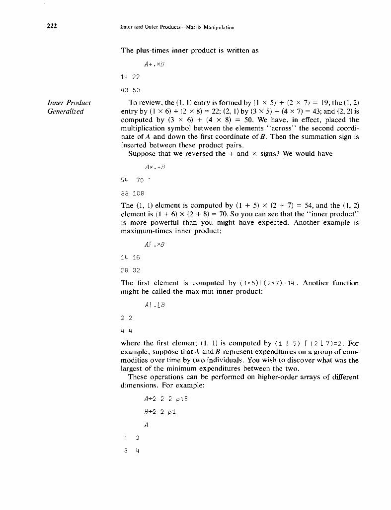
222
Inner ProductGeneralized
Inner and Outer Products-Matrix Manipulation
The plus-times inner product is written as
A+.xB
19 22
43 50
To review, the (1,1) entry is formed by (1 x 5) + (2 x 7) == 19; the (1,2)entry by (1 x 6) + (2 x 8) = 22; (2, 1) by (3 x 5) + (4 x 7) == 43; and (2,2) iscomputed by (3 x 6) + (4 x 8) == 50. We have, in effect, placed themultiplication symbol between the elements "across" the second coordinate ofA and down the first coordinate ofB. Then the summation sign isinserted between these product pairs.
Suppose that we reversed the + and x signs? We would have
Ax.+B
54 70"
88 108
The (1, 1) element is computed by (1 + 5) x (2 + 7) == 54, and the (1, 2)element is (1 + 6) x (2 + 8) == 70. So you can see that the "inner product"is more powerful than you might have expected. Another example ismaximum-times inner product:
14 16
28 32
The first element is computed by (1 x 5) r (2x 7) =14. Another functionmight be called the max-min inner product:
Ar. LB
2 2
4 4
where the first element (1,1) is computed by (1 L 5) r (2 L 7)=2. Forexample, suppose that A andB represent expenditures on a group of commodities over time by two individuals. You wish to discover what was thelargest of the minimum expenditures between the two.
These operations can be performed on higher-order arrays of differentdimensions. For example:
A+2 2 2 pl8
B+2 2 p1
A
1 2
3 4

12.2 Outer Product 223
5 6
7 8
B
1 1
1 1
A+.xB
3 3
7 7
11 11
15 15
The shape of the result of this command is 2 2 2. The shape always dropsthe last coordinate of the array on the left and the first coordinate of thearray on the right. The 1ddropped" coordinates must be equal to eachother-this is called conformability of the two arrays. Just as before, themultiplication symbol is placed between the elements of the last coordinateofA and the first ofB.
(1 x 1) + (2 x 1) = 3(3 x 1) + (4 x 1) = 7
(5 x 1) + (6 x 1) = 11(7 x 1) + (8 x 1) = 15
(1 x 1) + (2 x 1) = 3(3 x 1) + (4 x 1) = 7
(5 x 1) + (6 x 1) = 11(7 x 1) + (8 x 1) = 15
12.2 Outer Product
Outer Producto .fn.g
Another operation is illustrated by the following example. If we wantedto obtain the matrix product of the matrix in plane one ofA with that of thematrix in plane two of A, we would key in
A [ 1 ; ; ] + • xA [ 2 ; ; ]
19 22
43 50
This is exactly what we obtained in the first example of this section. If thetwo planes represent observations on two vectors of random variables,each observed over time, then the above operation produces the raw moment matrix of the random variables. Thus the typical (i, j) element of theiIlner product is mathematically LkXikYjk, where x ik and y jk are the kthobservations on Xi and yj, the ith andjth elements, respectively, in the xand y vectors of random variables.
This instruction enables you to place a primitive dyadic function betweeneach element in the corresponding positions in the two arrays. (Is that a

224 Inner and Outer Products-Matrix Manipulation
mouthful of words! And only a few weeks ago you didn't even know thatAPL means A Programming Language!) This function is constructed withtwo symbols, the null or jot (the little 0 above the J)and the period. Itsgeneral form is
Ao. fn B
where A and B can be either scalars or matrices. o. is called "jot dot."One use that is made of this instruction is preparing tables. Here is an
example of a simple arithmetic table for addition.
1 2 3 4 5 0 .+0 1 2 3 4 5
1 2 3 4 5 6
2 345 6 7
345 6 7 8
4 5 6 789
5 6 7 8 9 10
The first row is computed by adding to one (the first element on the left) allthe elements on the right of the outer product function. The second row isformed by adding the second element of the left argument to each elementof the right argument. Here is another way to visualize the operation:
+ 0 1 2 3 4 5
1 1 2 3 4 5 62 2 3 4 5 6 73 3 4 5 6 7 84 4 5 6 7 8 95 5 6 7 8 9 10
Notice that we have written in the column and row headings and theaddition symboL Let's try another simple arithmetic table, only this timelet B be a three-dimensional array.
B+2 2 2p 4+1.8
B
3 2
1 0
1 2
3 4
C+-O 1 2 o .xB
C

12.3 An Economic Example (Production Functions) 225
0 00 0
0 00 0
3 21 0
1 23 4
6 4
2 0
2 4
6 8
pC
3 2 2 2
Block 1, given by 0 x B
Block 2, given by 1 x B
Block 3, given by 2 x B
Notice that the shape that results from the outer product is the catenationof the shapes of the arrays A and B, P (A) == 3, P (B) == 2 2 2. C has 3blocks of 2 planes of 2 rows by 2 columns. The arithmetic is just as easy asit is in the simple case. The scalar zero is multiplied by every element ofthe three-dimensional array B, then 1 x B is formed, and then 2 x B. Feelfree to experiment with other dyadic operators or combinations ofoperators. However, be aware of how much storage, printing, and computer time you are using, since this is a "super-powerful" command.Consider how many values A 0 • *B would generate if the shapes ofA and Bwere each (5 5 5 5).
12.3 An Economic Example (Production Functions)
An interesting use of outer product concerns production functions. Suppose that we have estimated the parameters of a productioll function andwe want to examine the properties of the estimated function. We start witha modified version of a Cobb-Douglas production function:
and our estimates of the parameters could have been
Yi == 120.0 Lp·5Kp·5eO.3D i
Y; might be the amount of oil pumped from various drilling platforms, L;equals the amount of labor at each platform, K i is the amount of capitalservices at each of the platforms, and D i is a binary variable that takes onthe value 1 for offshore rigs and 0 for onshore rigs. Y is the estimate of theconditional mean of Y i • The Greek letters arJrsymbols for the parametersthat were estimated, and U i is a disturbance term distributed normally withzero mean and constant variance.

226 Inner and Outer Products-Matrix Manipulation
Our objective is to explain the economic implications of this equation.We write an APL program using the outer product command.
VPROD
[1J Y~120x(*0.3xD)o.x(L*0.5)o.x(K*0.5)
[2J \}
Working from right to left we raiseK to the 0.5 power. Next perform outerproduct multiplication with L raised to the 0.5 power. This twodimensional result is combined with eO.3D using the outer product multiplyagain. The final three-dimensional array is multiplied by 120.
Notice that we did not code the equation exactly as it was first written.Since the first dimension of the result is the coordinate of the left-mostvariable, we putD on the left. This allows us to see most easily the effect ofdrilling location on productivity. We generate some hypothetical data:
L+110
K+15
[frO 1
PROD
y
120 169.7056275 207.8460969 240 268.3281573
168.7056275 240 293.9387691 339.411255 379.4733192
207.8460969 293.9387691 360 415.6921938 464.7580015
240 339.411255 415.6921938 480 536.6563146
268.3281573 379.4733192 464.7580015 536.6563146 600
293.9387691 415.6921938 509.1168825 587.8775383 657.267069
317.4901573 448.9988864 549.9090834 634.9803147 709.929574
339.411255 480 587.8775383 678.8225099 758.9466384
360 509.1168825 623.5382907 720 804.9844719
379.4733192 536.6563146 657.267069 758.9466384 848.5281374
161.9830569 229.078636 280.5628845 323.9661138 362.2051265
229.078636 323.9661138 396.7758364 458.1572719 512.2354022
280.562845 396.7758364 485.9431707 561.1257691 627.3576818
323.9661138 458.1572719 561.1257691 647.9322276 724.4102529
362.2051265 512.2354022 627.3576818 724.4102529 809.9152845
396.7758364 561.1257691 687.2359079 793.5516728 887.217742

12.3 An Economic Example (Production Functions) 227
428.5668852 606.0851014 742.2996196 857.1337704 958.3046882
458.1572719 647.9322276 793.5516728 916.3145438 1024.470804
485.9491707 687.2359079 841.6886536 971.8983415 1086.615379
512.2354022 724.4102529 887.217742 1024.470804 1145.39318
The array Y has too many digits in each number for us easily to see whatis happening. Let's get an array of approximations to Y that will be easierto read. Let's try
YI+LY
YI
120 169 -
168 240
207 293 -
240
This array has the following form:
On-shore
Off-shore
[~~~~~~~~~~~~~~~JIncreasing~
IncreasingL
First Table Entries
[~~~~~~~~~~~~~~~)Increasing~
IncreasingL
Second Table Entries
You might also want to see the effect that an increase in the output elasticity of capital from 0.5 to 0.7 would have on output with various combinations of inputs. Consider
VPROV[lJ
[lJ [10J
[1J Y+120 x(*0.3 xD)o.x(L*0.5)o.x(K*0.5)
[1J Y+120x(*0.3 xD)o.x(L*0.5)o.x(K*O.7)
[2J V
228 Inner and Outer Products-Matrix Manipulation
PRG'-',D
LY
120 194 258 316 370
169 275 366 447 523
207 337 448 548 641
240 389 517 633 740
268 435 578 708 827
293 477 634 775 906
317 515 685 837 979
339 551 732 895 1047
360 584 776 950 1110
379 616 818 1001 1170
161 263 349 427 499
229 372 494 604 706
280 455 605 740 865
323 526 699 854 999
362 588 781 955 1117
396 644 856 1047 1224
428 696 924 1130 1322
458 744 988 1209 1413
485 789 1048 1282 1499
512 832 1105 1351 1580
These data can be plotted to give a clearer picture of the results.You have seen to some extent how higher-order arrays can be used in
APL to simplify your statistical calculations. However, it is easy to become confused at first. It will help you to avoid confusion if you experiment with small samples of data and check your work at each stage. Wehave kept the examples small so that they were relatively easy to check byhand. The last example on the prodiIction function was more ambitious,but now you are at a point where you can probably use APL to check yourAPL. Applications that are even more ambitious, but more useful, will bediscussed next.

12.4 Two More Not-So-Elementary Matrix Operations
12.4 Two More Not-So-Elementary Matrix Operations (KroneckerProduct, Determinant)
* Kronecker Product
229
KroneckerProduct
Later on, if you continue to study econometrics and statistics, you willfind a great need for a mathematical operation called the Kronecker product. The Kronecker product of two matrices I and W is written mathematically as I ® W, where I and Ware square matrices of dimensions (n x n)and (m x m), respectively. The result, say C, is of dimension (nm x nm),and is defined by
0"11 W 0"12 W0"21 W 0"22 W
C=2:®W==
O"nn W
where Land Ware the matrices
O"In
0"2n
O"tl 0"12
0"21 0"22
L=
O"nt O"n2
W=
W ml W mm
and O"ijW represents scalar multiplication of the matrix W by the scalar O"u.
This may at first glance look like a complicated product to obtain, but bynow you know that in APL the required computation will be easy. We usethe outer product introduced earlier in this chapter.
Consider first the straightforward multiplicative outer product A 0 • xB,which multiplies each element of the matrixA by each element ofmatrixB.So far so good. But the dimensions of the result are not exactly what arewanted. If D is the result of A 0 • xB, where A is (n x n) and B is (m x m),thenD has dimensions (n n m m), that is, n blocks ofn planes ofm rows andm columns, or we have n-squared (m x m) matrices. You may recall thatthe shape of A 0 • xB is the catenation of the shapes ofA and ofB. Blit wewant an (mn x mn) matrix. The desired rearrangement of the result can beachieved by using reshape and the dyadic transpose, ~ (key upper shift 0,backspace, key \).
As you will recall, the monadic transpose, when applied to a matrix,transposes rows and columns, but what about this strange beast of a multidimensional array D? QD would merely give us m blocks of m planes ofn x n matrices; the order of dimensions is merely reversed. Thus, to getwhat we want, we need to do two things: rearrange blocks, planes, rows,and columns so that then we can reshape the result to get an (mn x mn)matrix.

230 Inner and Outer Products-Matrix Manipulation
Let's consider the problem of getting A x B, where
lJ(3 x 3)
A (1 2)(2 x 2) - 3 4 l: ~ i]
First, let's see what the outer product gives us (assign values to A andB first!):
Block 1
Block 2
this is equivalent to allB
this is equivalent to a12B
this is equivalent to a21B
234
111
2 42 62 8
~ 1~ 1:)
:4 ~~8 16:) this is equivalent to a22B
If we try to reshape the above as it stands, we get the wrong results; tryit and see. The solution we want is obtained by use of the dyadic transpose.Our solution is given by recalling that if we label the positions in A 0 • xB by[I; J; K; L], we want to rearrange them so that we get instead [I; K; J; L], toget 2 blocks of 3 planes of 2 rows by 3 columns, which can now be reshaped into a (6 x 6) matrix. Consider then
1 3 2 4 ~D
If you type this into the computer and look at the output, you will observethat raveling the result (which proceeds by raveling the first matrix in thefirst plane in the first block, then the second matrix in the first plane in thefirst block), you will get an array that can be reshaped into that required forthe Kronecker product. Let's see it.
6 6 pi 3 2 4 ~D
1 2 4 2 4 8
1 3 3 2 6 6
1 4 2 2 8 4
.... . . ... ... .. ..... ..3 6 12 4 8 16
3 9 9 4 12 12
3 12 6 4 16 8

12.4 Two More Not-So-Elementary Matrix Operations 231
Determinant
The dotted lines have been inserted to aid you in relating the output to thedefinition of a Kronecker product.
Dyadic transpose gives us another advantage-an easy way to get thediagonal elements of a matrix. Let K be defined by
K+6 6 01 3 2 4 0D
Try
1 1 ~K
1 3 2 4 12 8
In short, using 1 1 ~ is how to get the diagonal elements of a matrix.The trace of a matrix is the sum of its diagonal elements, so that in APL
the trace is
+/1 1 ~K
30
Determinant
The next matrix operation you may need is the determinant, written asIAI. The determinant of a square matrix A of dimension (n x n) can bewritten as a linear function of determinants of submatrices ofA of dimension (n - I) x (n - 1); in short, the determinant can be defined for n = 1by A itself. For n == 2, IAI is given by (a 11a22 - a12Q 21 ). For larger n, if we letAu == (-I)i+iDih where D u is the determinant of the matrix obtained fromA by deleting the ith row andjth column, and let Qu be the (i,J)th elementof A, then
IAI = LJ=lQ tAufor any i = 1, 2, ... , n. This is the usual expansion by minors, which wecan program quite easily in APL. Let's begin by writing things out usingpaper and pencil.
We see that the routine for calculating the determinant can be decomposed into two main components: the calculation of the determinant of a2 x 2 matrix, and the recursive definition of a determinant of a matrix ofdimension n in terms of determinants of matrices of dimension (n - 1). Sothe basic elements of the routine are these two components, plus a decisioncomponent that enables the computer to know which of the other twocomponents to calculate.
The determinant of a 2 x 2 matrix is easily programmed. Consider
D+(x/1 1 ~A)-A[1;2JxA[2;1J.
D
2
which is nothing more than the APL version of (Q 11 Q22 - Q12 Q 21). You will

232
Looping
Inner and Outer Products-Matrix Manipulation
recall that 1 1 ~ A gives the diagonal elements ofA, so adding xl yieldsthe product of the diagonal elements.
If E is a vector containing the signs associated with the minors D Ij, thatis, E is a vector with elements 1 -1 1 -1 ... generated by (-I)i+j forj = 1, 2, ... , n, then the recursive definition is
~A[1;J +.x (ExM)
which is the APL version of
~n (-l)l+jD - ~JI A"~j=2alj Ij - ~j=lalj Ij
Looping
We note from our definitions that the vector M has to be created elementby element by getting the determinant of various submatrices. In short, toevaluate the function determinant, our function has to call itself! Fortunately, in APL this causes no difficulties, provided that it is done correctly. We also see that we have to do the same thing (n - 1) times (for ann-dimensional matrix) each time we call the function; this is called' 'looping. "
In order to define M, we have to calculate the determinants of thematricesA tt ,A I2 , ••• ,A ln , whereA is the matrix which is the argument ofour function. A Ij, you will recall, is obtained from A by deleting the firstrOHJ and thejth column. To do this in APL, we will need to use the indexingof arrays and the "drop," ~', operation (key upper shift U). Anotheroperation we need in this routine is "compression," which is the dyadicuse of I.
In our problem we want to drop only one row (the first) and one column,but a different one each time; this is where the indexing comes in. If werearrange the matrix A so that the column to be dropped is first, and if wekeep everything else in the same order, you can easily see (at least by usinga paper and pencil to try it) that this will give us the submatrices we want.Consider the following:
N+-1 01 pA
IND+1N
)ERASE B
B+-(N,N) pO
B
0 0
0 0
{We need to know how "big" A is.
{Gives us the index numbers 1,2, ... ,N.
{We need a "dummy" matrix forreindexing.
I +-1 {Initializes our index.
{Produces an index array
IN+( I ~IND) lIND with the I th element deleted.
M+-M, DET 1 1 +B[ ; INDJ+-A [ ;I ,IN]

12.4 Two More Not-So-Elementary Matrix Operations 233
'[he last line needs some discussion. First, let's call our determinant function DET and let it have one argument, the matrix whose determinant weare trying to obtain. Also, by writing M+-M ,DET (argument), we create a listM with determinants as its elements by catenation.
B[ ;INDJ+A[;I ,IN]
rearranges the columns ofA so that the column to be deleted, indexed by I,occurs first inB, and the remaining columns are unchanged in their relativepositions. l1-rB deletes the first row and column of B, and DET takes thedeterminant; in short, we get the (1, I) minor by this line.
We are nearly done-the next most important step is to complete thelooping through the index I from 1 to N. This is done as follows:
I+l {Initializes the loop.
{Gets us out of the loop
ST:-+ST1 x l(I> N) when! exceedsN.
IN+-(I~IND)/IND
M+-M,DET 1 1 -rB[;INDJ+A[;I,INJ
E+E, (-1*(1+I) ) {Produces the vector of signs.
I+I+l {Increments I for the looping.
{Takes us back to the be
-+ST ginning to check on I.
We now have only a few minor details to settle: the original decision ofwhether to go to the n = 2 case and some "housekeeping chores." Forexample, in order to define M and E in the way in which we have done it,they have to be "defined as lists," even if there are no elements in them.This is done by setting MoE-tO and E-4:- LO.
The whole routine is
VD+DET A;N;E;I;IN;IND;M;B
[1J N+1 0 / pA
[2J -+ENDx l(N=2)
[3J IND+-1N
[4J B+(N,N)pO
[5J I+1
[6J ~10
[7J E+10
[8J ST:-+ST1 x l(I > N)
[9J IN+-(I~IND)/IND
[10J ft¥-M,DET 1 1 -rB[ ;INDJ+A[;I ,IN]
[11J E+E, ( -1 ) * (I + 1 )
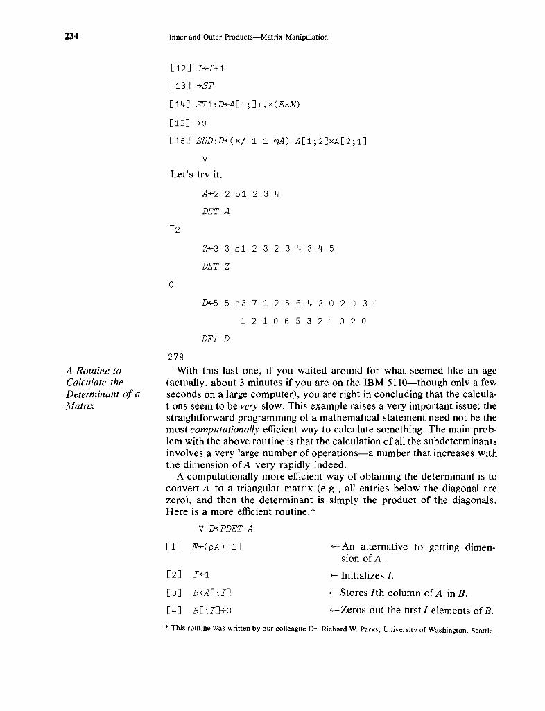
234
A Routine toCalculate theDeterminant of aMatrix
Inner and Outer Products-Matrix Manipulation
[12] I+I+1
[13J -+ST
[14J ST1:D+A[1;J+.x(ExM)
[15J -+0
[16J END:~(x/ 1 1 ~A)-A[1;2JxA[2;1J
V
Let's try it.
A+2 2 pi 2 3 4
DET A
2
Z+3 3 pi 2 3 2 3 4 3 4 5
DET Z
a
D+5 5 p3 7 1 2 5 6 4 3 0 2 a 3 0
1 2 1 0 6 5 3 2 1 0 2 0
DET D
278
With this last one, if you waited around for what seemed like an age(actually, about 3 minutes if you are on the IBM 5110-though only a fewseconds on a large computer), you are right in concluding that the calculations seem to be very slow. This example raises a very important issue: thestraightforward programming of a mathematical statement need not be themost computationally efficient way to calculate something. The main problem with the above routine is that the calculation of all the subdeterminantsinvolves a very large number of operations-a number that increases withthe dimension ofA very rapidly indeed.
A computationally more efficient way of obtaining the determinant is toconvert A to a triangular matrix (e.g., all entries below the diagonal arezero), and then the determinant is simply the product of the diagonals.Here is a more efficient routine.*
V ~PDET A
[1J N+( pA) [1J ~An alternative to getting dimen-sion of A.
[2J I+1 ~ Initializes I.
[3J B+A[ ;IJ ~Stores lth column of A in B.
[4J B[ lIJ+o ~Zeros out the first I elements of B.
* This routine was written by our colleague Dr. Richard W. Parks, University of Washington, Seattle.

Summary
[5J A+A-(Ba.xA[I;J)~A[I;IJ
[6J ~(N~I+I+1)/3
[7J D+-x/ 1 1 ~A
235
-E-See below.
-E-See below.
~Obtains determinant by multiplying the diagonal elements.
Summary
Only lines [5] and [6] require any explanation. The main idea of thisroutine's algorithm (method of calculating a mathematical formula) occurs in line [5]. The idea is to transform the matrix A into a triangularmatrix; in this case all elements below the diagonal are zero. This is accomplished by subtracting from each row ofA the elements ofA to the leftof the diagonaL
Line [6] increments the index I and then returns to line [3] if N 2: I;otherwise we continue to line [7] to calculate D.
PDET Z
o
PDET D
278
If you try this routine, you will find that it will execute the matrix D muchfaster than does the previous routine. Indeed, on the IBM 5120 it will dothe D matrix in about 7 seconds. However, even this routine has its problems, since it will not work if any of the diagonal elements are zero.
While this lesson may have been a bit expensive, the lesson to be learnedis important. As your routines become more complex, you will have toworry about computationally efficient ways of handling the problem. Finally, you should realize that the usual mathematical statements, whilevery informative, can often be computationally inefficient.
Inner Product and Multidimensional Arrays: the general form ofthis product is Afn t • fn2B, where A, B are arrays, andfnl,fn2 are functions.For example, A+. xB where A , B are two arrays, gives the usual mathematical operation of "matrix product." The inner product for multipledimensional arrays is always between the elements of the last dimension ofA and the elements of the first dimension of B.
Outer Product, o.fn (keyed by upper shift J, period, followed by afunction): general use is given by A a •.fn B where A, B are arrays. Theoutput is an array whose dimensions are the catenation of the dimensions ofA and ofB. Each element ofA is an argument to the dyadic functionfn forevery element ofB.
Kronecker Matrix Product: mathematically is given by L ~ W,where Land Ware (n x n) and (m x m) matrices, respectively. The result
236
Exercises
Inner and Outer Products-Matrix Manipulation
is of dimension (nm x nm) and each element of ~ scalar multiplies thematrix W The Kronecker product, K, for two matrices A, B is obtained inAPL by
MN+(N+1 0/ pA)x(l\¥-1 0/ pB)
K+MN MN p1 3 2 4 ~Ao. xB
Determinant of a square matrix A, denoted by IAI: defined mathematicallyby
IAI = ~f=laijAij, fot any i == 1, 2, ... , n.Qij == (i, j)th element of AAu == (-l)i+jDuD ij == IAul, called the Cij) minor of A.Au == matrix A with ith row andjth column deleted, is the (ij)th
cofactor of A .
Two illustrative APL routines are given in the text; care is needed in theuse of both.
APL Practice
1. ForanylistL, the APL expressions L~«pL), 1)p'1 andLfBI,fLgivethe same number. What is this number? Why is this result true?
2. For two positive numbers A and B, the APL expressions«A*2 )+B*2)*. 5 and AX40B~A give the same number. What is thisnumber? What is the explanation?
3. IfX+--o(0,t12)f12 and Y*Q 123 o.oX,whatisinY?
4. LetM be any matrix and L+( ,M>K) /, M where K is any number. Whatis in L?
5. Let Qy?N p K and F++/[l]Qo. =lK for any two positive numbers Nand K. What is in F?
6. Use the outer product to construct the following tables.
(a) A table 100 by 10 of the powers from 1 to 10 of the integers from 1to 100.
(b) A table 100 by 2 of the logarithms to base e and base 10 of theintegers from 1 to 100.
(c) A table 100 by 10 of the 1st through the 10th root of the integersfrom 1 to 100.
(d) A table of all possible products of the integers from 1 to 30.
(e) A table of the binomial coefficients (ji=l) for i <j andj = 30. (Seeexercise 9, Chapter 11.)
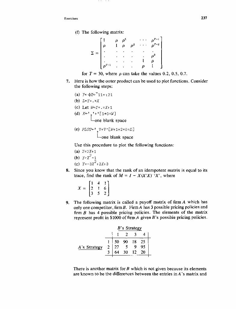
Exercises
(t) The following matrix:
237
1p
pT-l
p21 pp 1
for T = 30, where p can take the values 0.2, 0.5, 0.7.
7. Here is how the outer product can be used to plot functions. Considerthe following steps:
(a) Y+-¢X+-l1+121
(b) L+Yo. xX
(c) Let W+Yo. =X+1
(d) K+' '+' [l-tO=W]
Lone blank space
(e) PLOT+' V+'V· [W+1+2 x O=LJ
Lone blank space
Use this procedure to plot the following functions:
(a) Y=2X+1
(b) Y=X2-1
(c) Y=-3X2
+2X+3
8. Since you know that the rank of an idempotent matrix is equal to itstrace, find the rank of M = I - X(X'X)-lX', where
X = [~ i ~]352
9. The following matrix is called a payoff matrix of firm A which hasonly one competitor, firmB. FirmA has 3 possible pricing policies andfirm B has 4 possible pricing policies. The elements of the matrixrepresent profit in $1000 of firmA givenB's possible pricing policies.
B 's Strategy
123 4
1A's Strategy 2
3
50 90 18 2527 5 9 9564 30 12 20
There is another matrix for B which is not given because its elementsare known to be the differences between the entries inA's matrix and

238 Inner and Outer Products-Matrix Manipulation
100 (assuming that only $100,000 profit can be made in the market). IfA chooses strategy 1, then B will choose strategy 3, because B gets$82,000, which is the highest profit for B given A 's strategy. Thus A'sone optimum policy (called maximin) is to find the minimum of eachrow and then pick the maximum of those minima. This long verbalstory is only half a line in APL. Can you write it? What if A choosesa minimax strategy? (A minimax strategy is exactly the opposite tothe maximin strategy.)
10. Consider the following table:
Table M
Possible home mortgage ratevalues this year in %
10.50 11.00 11.50 11.75
Possible home 10.50 0.1 0.25 0.4 0.25mortgage rate 11.00 0.25 0.3 0.25 0.20values next 11.50 0.4 0.25 0.1 0.25year in % 11.75 0.25 0.20 0.25 0.3
Each element of this table represents the probability of next year'sinterest rate given the rate this year. Notice that column and rowelements sum to 1. Enter the matrix of probabilities into the variableM.
(a) Find next year's expected interest rate if this year's interest rateis 11.50%.
(b) Find next year's expected interest rates under all possible alternative values for this year.
(c) Let
10.511.011.511.75
Then Mr( will be a vector of next year's expected values given thisyear's alternatives. Let's call this vector rt+l. Then r(+2 = Mrt+t willbe the potential values in year rt+2.Give alternative interest rates foryear t + 1. Project possible interest rates up to 5 periods ahead. Dothey seem to converge to an equilibrium value?
11. Enter both routines DET and PDET in your workspace (see pages233-235) and find the determinants of the matrices
(a) A = [; ;~] (b) B = [~ ~ ;]
313 112(c) AB

Exercises 239
(d) A @ B, where ® is the Kronecker product.
(e) B ®A
12. Using the PDET A function (page 234), solve the following system ofequations utilizing Crammer's rule, which is explained below:
2X + 3Y - 3Z = 7
X - 2Y + Z = -2
3X + Y + Z = 9
Solutions by Crammer's rule are given by:
X= axa'
y= ay
d'Z = ~z
awhere~ is the determinant of the matrix of coefficients.~x is the determinant of the matrix a with the first column replaced
by the column of constants.~y is the determinant of matrix a with the second column replaced by
the column of constants.Az is the determinant of the matrix a with the third column replaced
by the column of constants.
13. Let C+-1+?10 P2. Examine carefully the results of the following operations.
(a) 21\C
(b) 1ve
(c) ave(d) C+. /\c(e) Co .I\C
(f) Co.¥C
(g) Co .'!'<C and compare to (e).
(h) Co. vC and compare to (f).
14. (a) Assign the statement "'I don't like APL and tea" to variable X.
(b) Write an APL function that will erase the n, the apostrophe andthe t of the word don't using the logical operators.

13
Linear Regression
For those of you who already know a fair amount of statistics, here is thechapter you have been waiting for. Now is the time to come to grips withregression analysis, the calculation of confidence intervals, and tests ofhypotheses. In this chapter you will learn the advantages of being able todo all your statistical analysis yourself instead of relying on someone else'sblack box. Before you proceed, you might want to refresh your memoryabout simple linear regression (Chapter 9) and the use of Iil (Chapter 10).
This chapter deals only with the analysis of single-equation (as opposedto multi-equation), and linear (as opposed to nonlinear), regression equations. You might well be wondering why we have a whole chapter onregression, when the regression of a vector Y on a matrix X is obtained inAPL by Y fB X. The answer is that there are a number of associatedstatistics with a linear regression which need calculation and these are alittle messier computationally. Let's begin.
13.1 Covariance and Correlation Matrices...
Moment,Covariance andCorrelation Matrices
240
The basic input to any regression problem is an (N x K) matrix of Nobservations on K regressors (variables used to "explain" the dependentor regressand variable Y). An important set of statistics for many reasons isthe sample moment, covariance, and correlation matrices. If X is the
•

13.1 Covariance and Correlation Matrices 241
Simple CorrelationMatrix of Regressors
(N X K) regressor matrix, the mathematical statements are, In matrixterms,
Moment matrix X'XCovariance matrix X'X - X'XCorrelation matrix D-1/2(X' X - X' X)D-1I2
where you may recall that X'X is the inner product between X transposeand X itself, X is an N x K matrix, each of whose rows contains the arrayof means of the K regressors, and D is a diagonal matrix whose ith diagonalelement is the variance of the ith regressor variable, so that D-1/2 is thediagonal matrix of the inverse of the square roots of the nonzero elementsofD.
The above mathematical equations give the matrix equivalents of thevariances and covariances we calculated in Chapters 5 and 9. Each ofthese matrices is easily obtained in APL. They are, in turn,
Moment matrix: ~(~X)+. xXCovariance matrix: CM+-MM- (XB 0 • xXB-H-/X) -i- CpX) [1 ]Correlation matrix: CRJi,¥.D+. xCM+ • xl)+-illC ( ( lK) 0 • = lK-+-( pX) [2] )
xCM)*O.5
Let's explain this. The moment matrix is easy: ~X produces X transpose and (~X) +. x X gives the inner product of ?siX with X. Thecovariance matrix introduces something we used briefly in Chapter 9,namely (pX) [1] , which means: shape ofX over the first dimension, inshort, the number of rows. The rest is easy to understand once you realizethat x'X, whereX' is an (N x K) matrix of the means of the K variables, issimply N (== number of rows == (pX) [1J) times the outer product of thearray of means, or 1/N times the outer product of the vector of columnsums ofX.
The correlation matrix is obtained from the covariance matrix by dividing the covariance between the ith andjth variables by the product of thestandard deviations (square roots of the variances) of the ith andjth variables. The variance of the ith variable is clearly given by the ith diagonalterm of eM. The elements of CRM. usually labelled in mathematical notation as Pu == COV(Xi' Xj)/VVar(Xi)Var(Xj) , satisfy the mathematical constraint -l$Pu:5 1. For further mathematical and statistical details seeMendenhall and Reinmuth or Kmenta, both of which are listed in thebibliography at the end of the book.
The APL expression is now fairly obvious. K is the number of regressors. ( lK) 0 • = lK) xCM produces a diagonal matrix with the diagonal elements of eM, and m( (( 1 K) 0 • =tK) xCM) * . 5 gives the inverse of thesquare roots of the variance obtained from the CM matrix; the reason thatwe cannot use *-0. 5 is that the zero off-diagonal terms will giveDOMAIN ERROR. The operation D+. xCM+. xD produces a matrix with Pu onthe off-diagonal positions and 1's on the diagonal.

242 Linear Regression
For example, let us suppose that we have the following X matrix in thecomputer's memory:
x(12 x 2)
1009080707070706560605550
5.506.307.207.006.307.355.607.157.506.907.156.50
and if we don't, let's enter X now.Consider a simple routine to calculate the moment matrices that we have
been discussing.
'V M4TCO] 'V
\jCR~MAT X;D;MM;CM;K;XB
[1J 'MM EQUALS';Mru+(~X)+.xX
[2J 'eM EQUALS';C~MM-(XBo.xXB++fX)+(pX)[1J
[3J K+(pX)[2]
[4J 'CRM EQUALS'
[5J CRM+D+.xCM+.xD+ffi(((lK)o.=lK)xCM)*O.5
MAT X
MM EQUALS
61050
5577.5
eM EQUALS
2250
54
5577.5
544.2075
54
4.857291667
CRM EQUALS
1 0.5165417262
0.5165417262 1
And if we have the following three-column regressor matrix:
zzz

13.2 Some Initial Linear Regression Statistics
55 100 5.5
70 90 6.3
90 80 7.2
100 70 7
90 70 6.3
105 70 7.35
80 70 5.6
110 65 7.15
125 60 7.5
115 60 6.9
130 55 7.15
130 50 6.5
Our routine produces:
MAT ZZ
MM EQUALS
126300 80450
80450
8170.25
eM EQUALS
6300
3550
125.25
61050
5577.5
3550
2250
54
8170.25
5577.5
544.2075
125.25
54
4.85729166667
243
CRM EQUALS
1 0.942902569586 0.715995624984
-0.942902569586 1 0.516541726216
0.715995624984 0.516541726216 1
13.2 Some Initial Linear Regression Statistics
The first generalization of the regression model which was discussed inChapter 9 is to allow for more than one regressor; to some extent we havedone this already with the use of the function ffi. The general model to bediscussed in this chapter is

244 Linear Regression
Y = XB + U
where Y is an (N x 1) regressand vector, X is the N x K matrix of regressors, B is the K x 1vector of regression coefficients to be estimated, and Uis the N x 1 vector of unobserved disturbance terms. Excellent elementarydiscussions of multiple regression analysis can be found in both of thereferences mentioned on page 241.
From our work in Chapters 9 and 10, you know the least-squares approach to estimating the regression coefficients involves the calculation ofthe left inverse ofX. The left inverse ofX is (X' X) -1 X' (recall that ALI is theleft inverse ofA if ALIA ~ I) and in APL this is obtained by fRY, using themonadic use of domino. The least-squares regression coefficients are obtained by the dyadic use of domino, Y!±IX, which is the APL equivalent ofthe mathematical expression (X' X)-1 X' Y. Mathematically, we obtain from(X' X)-lX' Y the expression B + (X' X)-IX' u. The statistical properties ofthe least-squares estimator depend on the statistical properties of the vector (X' X)-lX' U. Let's store the regression coefficient estimators inBE, i.e.,we compute BE+-YI±lX; BE stands for B vector Estimate.
As we mentioned in the note to instructors, some computer systemshave not implemented the dyadic form of domino. An easy way around thisis to write your own function directly.
VY DQ X
[lJ (ffi((~X)+.xX))+.x((~X)+.xY)V
Here is how it works for a 3 independent variable case where the interceptis constrained to be equal to zero.
CLEAR WS
Y+-10?10
X+-10 3p30 ?30
0.076969 0.0021871 0.24941
(~ ((~X)+.xX) )+.x((~X)+.xy)
0.076969 0.0021871 0.24941
The estimator of the variance of the disturbance term was given for thespecial case examined in Chapter 9. The general mathematical expressionIS
where Y = xiJ, Y' = (Y t , Y2' . .. , Yn), where ;\ symbolizes the estimatorof the variable or parameter under the 1\. Thus fJ symbolizes the estimatorof B in the model Y = XB + V, where iJ == (X' X)-lX' Y.
The maximum-likelihood estimator of the variance of U is a little different, involving division by N instead of N - K. Vi is the forecast value of Y i
for the ith observation given the regression coefficient estimates, i.e., Yi =
13.3 Simple and Partial Correlation Coefficients 245
~f~r XijB j • Bj , j = 1, 2, ... ,K are obtained in APL by calculating thevector BE defined above. The APL expression for the estimator of thevariance of U is
NP+- pX
V +-(SSE+(Y-X+.xBE)*2)~(-/NP)
and in the process, we have defined the "error sum of squares," SSE,which will be needed later. Note that NP is the array (N, K), and - /NP issimply (N - K). Y is obviously given by X +. x BE.
The estimated covariance matrix of the regression coefficient estimatorshas two forms, depending on whether or not the regression equation is runin "deviation terms" [that is, after elimination of the "constant vector"i' = (1, 1, ... , 1) by subtracting the mean from each variable]. If theregression is run in deviation terms, the estimated covariance matrix forBE is given by
COVD +- V x eM
If the regression is not run in deviation terms, the estimated covariancematrix for BE is given by
I +- 1
RM +- (~Z) +.x Z +- I~X
COV +Vx RM
The dimensions of COVD are (K x K) and of COV, (K + 1) x (K + 1)),when there are K regressors in X. The use of the catenate function increating the matrix Z from I and X was discussed in Chapter 11.
The coefficient of determination (R 2) was defined in Chapter 9; the mul
tiple correlation coefficient is merely the square root of R 2• Note that the
coefficient of determination defined in Chapter 9 by I-SSE/SST gives thecoefficient of determination with respect to variables defined in terms ofdeviations about their respective means. If the R"2 value is wanted in termsof the original variables, then the new R 2 is defined as before, except thatSST is given by Y+.x Y instead of Y+.xY-((+/Y)*2)~N.
13.3 Simple and Partial Correlation Coefficients
Simple and PartialCorrelationCoefficients
A topic related to regression analysis is the analysis of simple and partialcorrelation coefficients. The simple correlation coefficient has already beendefined and calculated in this chapter. Given K variables, the simple correlation between any two of them, say the lth andjth, is given mathematicallyby fO = COV(Xi' Xj)/ VVar(xj)Var(xj); the simple correlation coefficient"measures" the extent of linear association between the two variables land}.
A related concept is the partial correlation coefficient, say rU'k, which isthe correlation between variables i and} a.fter allowing for the joint correla-

246 Linear Regression
tions between variables k and i and between variables k and j. The partialcorrelation coefficient can be obtained easily from the simple correlationcoefficients; mathematically, one has
rij'k = (rij - rikrjk)Iv(I - rTk) (I - rJk)
where 'ij, 'ik, rjk are the simple correlation coefficients.The matrix CRM obtained above gives for any set of K variables the
matrix of simple correlation coefficients between each of the K variables.Any partial correlation coefficient can be obtained from the CRM matrix.By now you should be able to program this on your own.
13.4 Creation of a Regression Routine
Let us now consider creating a reasonably complete regression routine.The procedure will not only provide us with our own regression routinewhich, of course, we can alter in any way at any time we like, but it alsowill provide some valuable lessons in how to write routines that are morecomplicated than those we have tackled so far. Let's begin at the verybeginning, which is to determine what we are required to do mathematically. Our next step will be to plan our programming steps. Here then is arecommended procedure for you to follow in writing any program routineof any difficulty.
1. Write down all the mathematical expressions needed; sequence theexpressions so that all operations to be completed before a particularstep are in fact listed before that step. One diagrammatic way to helpyou do this is to write down a flow chart, an example of which isgiven for the regression routine below.
2. Figure Ollt whether any loops or conditional branch statements areneeded and, if so, where in the program they are needed. Rethink thebasic APL approach to see if there are alternative ways to get resultswhich will not use up inordinate amounts of computer time andspace.
3. Decide for each function whether the result is to be explicit or implicit, have one or two arguments, and which variables, if any, are tobe globally defined.
4. Begin with paper and pencil and assemble the various parts of theroutine that may already be written out.
5. Using your flow chart, layout the sequence of "one liners" and setup your decision branches. As you do so, label all statements involving branches.
6. With each "one liner" expression, start with the "core" of the mathematical term and put it in the middle of the page; build outwards fromthere, and then recheck by reading the expression from right to left.

13.4 Creation of a Regression Routine 247
7. Alter the header line as you introduce local variables to avoid forgetting them.
8. Recheck yOUT program carefully, looking to see that:
(a) program statements give the results desired (read from right toleft!);
(b) the relationships between arrays, vectors, and matrices are comformable (possible length errors);
(c) every variable will be defined before it is used;
(d) loops, branches, and recursive function definitions will terminateunder all alternatives.
9. Document your routine very carefully and include explanatory comments inside it (within a month, you won't remember how you did it!).
10. Enter the routine into the computer, then enter several easy problemsfor which you have the answers in order to check that the routine iscorrect. Be sure that you check the routine for general, not justspecial, cases.
11. Remember, even when you believe it is impossible to make a mistake,you will!
You might well ask: Why all these elaborate instructions? Up until nowmost of our routines have simply been written out. The answer is that sofar the routines have all been very uncomplicated-the regression routineto follow is our first example of a more elaborate routine. Also, it is the firstroutine that we might want to keep for future use, so we need to be morecareful about how we define it and set it up for use by others.
The following routine is a suggestion; a lot of variables are global since itis assumed that the output will be used in further analysis. We need sometrial data. Let us suppose that the first column of ZZZ is the regressandarray 1': and the remaining two columns ofZZZ are the regressor matrixX.Thus
Y+ZZZ[;l]
X+ZZZ[;2 3J
Y
55 70 90 100 90 105 80 110 125 115 130 13a
x
100 5.5
90 6.3
80 7.2
70 7
70 6.3

248 Linear Regression
70 7.35
70 5.6
65 7.15
60 7.5
60 6.9
55 7.15
50 6.5
Let us begin to write out the regression routine by deciding on what it iswe want.
Desired Calculations
regression coefficient estimates
raw moment matrix
covariance matrix for regression coefficientsvariance of disturbance term U ~
R2 (the coefficient of determination)
correlation matrix for regressors
array Yarray 0 = (Y - Y)F statistics with degrees of freedomstandard deviations of the regression coefficient estimates
T ratios for the regression coefficient estimates
Disposition: all of the above to be global variables; but f: 0 to be printedout automatically; two arguments Y and X.
An examination of the formulas in Table 13.1 shows that there is a certain order in which calculations should be made and certain intermediateproducts which need to be defined as they are reused repeatedly. Whilethe mathematical structure of this routine is very simple and hardly callsfor an elaborate flow chart, one is given in Figure 13.1 in order to illustratethe idea. Our main concern is to keep the number of computations andnumbers of arrays to a minimum, the former to economize on computertime, the latter to economize on space taken up in the computer.
In the process of working up the flow chart, you can see that some ideasoccurred to us. First, we should remember that a function or a routine isdefined for general use, so you should be on your guard to watch out forproblems caused by someone trying to do something which you did notanticipate. The first decision box illustrates this problem. Someone mayinadvertently specify an X matrix with more variables than observations(more columns than rows). If no test is made for this mistake, the com-

13.4 Creation of a Regression Routine
Table 13.1 List of Mathematical Expressions and Tentative APL Statements
249
Definition
Moment matrix ofXCovariance matrixof XCorrelation matrixof X(D is the diagonalmatrix obtainedfrom Cov(X»Regression coefficient estimators:
Total Sum ofSquares (TSS)Error Sum ofSquares (ESS)Var (U)R2Regression SS(RSS)If donewithout constantterm:F = (RSS/ESS)/((N - K - l)/K)COY matrix forfJ, whereZ = (i, x)Standard deviations of elementsof B given bysquare roots ofdiagonal elementsof covariancematrix for fJ, S~Student 44(" ratios
Mathematical Expression
X'X
X'X- X'X
D-tl2(X' X - X' X)D-tl2
Diag(X' X - X'1)
fJ = (X'X)-tx'yy = xiJU=y-y~(Y - Y)2
L(Y - Y)2 = 'L,U 2
'LUz/(N - K - 1)1 - ESS/TSS'L,(Y - Y)2
var (U)(Z' Z)-l
S~ = (Diag Cov(B»
fJ i/SBi, i = 1, 2, . . . ,k
APL Expression
~({QX)+.xX
CM+-MM- eXBo. xXB++fX) -;- (pX)
CRM+D+ . xCM+ . xD
+ffi(((lK)o.=lK+(pX)[2])xCM)*O.5
BE+.YtEXYH+X+.xBEUH+Y-YHTSS++/(Y+YB)*2YB+( +/ Y) -;-pYESS++/UH*2
VARU+ESS+ (N-K+1)RSQ+1-ESSfTSS
RSS++/(YH-YB)*2
F+(RSS~ESS)x«N-K+l)+K)
COVB+VARUx~«~Z)+.xZ)
SBE+( 11~COVB)*O. 5
TRATIO+-BE~SBE
puter will blithely proceed to the calculation of the regression coefficientsand then give a DOMAIN ERROR and specify the line in the program atwhich the error occurred. This is all very well, but you may want theprogram which contains the regression routine to continue in any case andnot stop. If so, a diagnostic test will get you around the difficulty beforeyou waste valuable computer time. In addition, you can specify a warningvariable to indicate when the regression routine has not, in fact, beenexecuted; this is called' 'setting a flag. "
The second idea is that sometimes we want to carry out the F test on themean as well as on the statistical significance of the regression coefficientsfor the regressor matrix, so we have allowed for two variants of the test:
and

250
Figure 13.1Flow chart for regression routine.
Linear Regression
,---IIII
-No------~
i O
x,yX'X - xl:i0
correl Mat. X, fYl
yO:t, y2'
BEYHUH
TSSOESSoRSSoRSS~'
RSQO
VAR UCO VBE
St. Dev. BEo
Student I ratiosi,ix'xCovxCorrel. xBESt. Dev. BE, RSQCO VBEVAR UF
"F2

13.4 Creation of a Regression Routine
Sample Main Sheet
V Y MREGRESS X;MS;D;SS
[1 J R THIS PROGRAM ASSUMES Y TO BE AN ARRAY OF DIMEN.
eN), x TO BE AN (NxK) ARRAY
[2J R OF PANK K. A DIAGNOSTIC IS PRINTED IF N5-K OR IF
RANK ex) <K.
[ 3J R THE CONSTANT TERM IS ADDED BY THE ROUTINE.
[4J NP+ pX
[5J PREMEND1xl(NP[1J~NP[2J+1)
[6J C~(MM+(~ X)+.xX)-(MSo.xMS++fX)+NP[1]
[7J CR~D+.xCM+~x~«(tK)o.=tK)xCM)*O.5
[4.2J K+NP[2J
[8J MS+(+/Y),MS)+NP[lJ
[9 J SS[2]+(SS[1J++/Y*2)-NP[1]xMS[1J*2
[4.5J SS+5 pO
[10J MWIN:UH+(Y-(YH+X+.x(BE+Yffi(X+(1,X)))))
[3.1J A**** IF DOMAIN ERROR OCCURS ON LINE [7J OR [ftMINJ
X IS SINGULAR 9 ROUTINE WILL BE SUSPENDED
[3.2J AOPERATOR SHOULD KEY IN: -+PREMEND
IN ORDER TO COMPLETE ROUTINE. ****
[llJ SS[4J+(SS[3J++/YH*2)-NP[1JxMS[1J*2
[12J SS[SJ++/UH*2
[13J RSQ+1-SS[5]+SS[2J
[14J VARU+SS[5]+(-/NP)-1
[1SJ F1+SS[4J+SS[S]xK+(-/N?)-1
[16J F2+SS[3J+SS[SJx(K+1)+(-/NP)-1
[17J COVBE+VARUx~(~X)+.xx
[18J STDBE+( 1 1 tQCOVBE) *0 •S
[19J 'THE RAW MOMENT MATRIX OF REGRESSORS. IS: '
[20J MM
[21J 'THE COVARIANCE MATRIX OF REGRESSORS IS: '
251

252 Linear Regression
[22J
[23J
[24J
[25J
[18.5J
[26J
[22.1J
[22.3J
CM
MAINEND: 'THE CORRELATION MATRIX OF REGRESSORS IS: t
CRM
'THE VECTOR OF MEANS; Y.,Xl,X1, .. •IS:'
TRATIO+-BE+STDBE
MS
-+MAINENDx 1FLAG
'ROUTINE PREMATURELY ENDED DUE TO SINGULARITY OF
X MATRIX'
-+0
PREMEND 1:'NO. OF OBS. (N) IS TOO FEW RELATIVE TO NO.
OF REGRESSORS (K).'
'ROUTINE TERMINATED'
[22.4J -+0
[ 3 . 4] FLAG+l
[18.1J -+CONT
[18 . 2] PREMEND: FLAG+- 0
[18 . 3 J[19 J CONT: 'THE RAW MOMENT MATRIX OF REGRESSORS IS: '
[30 J 'THE REGRESSION COEFF:!CIENT ESTIMATES ARE IN ORDER
CONST • ., X1,X2 .•. :'
BE
'THE CORRESPONDING STANDARD ERRORS ARE: '
STDBE
'THE REG. COEP. EST. COVARIANCE lv1ATRIX IS: '
COVEE
'RSQ IS: ';RSQ;' VAR. ERROR TERM IS: ' ; VARU
'THE F STATISTIC INCLUDING THE CONSTANT TERM IS: '
F2;' WITH' ;(K+1) ,!>(-l+-/NP); 'DEGREES OF FREEDOM. '
'THE F STATISTIC NOT INCLUDING CONSTANT TERM IS: '
P1; 'WITH ';K,("-l+-/NP); , DEGREES OF FREEDOM: '
THIS ENDS THE OUTPUT FROM MREGRESS. '
[44J
[31J
[32J
[33J
[34J
[35J
[36J
[37J
[38J
[39 J
[40J
[41J
[42J
[43J

13.4 Creation of a Regression Routine
[33. 5 J 'THE CORRESPONDING T RATIOS ARE: '
[33.7J TRATIO
[45J V
Sample Subsidiary Sheet
Used for Preliminary Working Out of APL Statements
253
Reline [4]: N+pX
+PREMENDxl(N[1J~N[2J+l)
Reline [6]: MM+C ~X) + . xXCM+MM-(MSo.xMS++IX)~N[1J
Reline [7]: CRM+-D+. xCM+ • xD+{fJ( ( ( lK) 0 • =lK+-N[ 2]) xCM) *0 . 5
Reline [8]: MS+( (+/Y) ~N [1J ,MS~N[lJ)
Reline [9]: TSS2+( TSS+-+ / Y*2 ) - NxMS[ 1 J* 2
Reline [10]: YH+-X+. x (BE+-Yl±](X+-( l.,X)))
At this point you could get a DOMAIN ERROR and a suspended routineif the augmented X matrix is singular. To get out of this and continueoperation will require operator intervention from the terminal; a flag mustbe set to bypass the remaining analysis and to print only what has beendone so far. Operator action is indicated in the comment lines labelled [3.1]and [3.2]. You will notice that we havejust realized that we could also get adomain error leading to a suspension in the current line [7]. (This is indicated on the flow chart by the dotted-dashed line which was added later.)
Reline [11]: SS[4]+-(SS[3J+-+/YH*2)-NP[1]xMS[1]*2
Reline [17]: COVBE+VARUx[±]( ~X) +. xX
Reline [18]: STDBE+-( 11 QCOVBE) *0 .5
Some of the early calculations not affected by the domain error can beprinted, but we will need to bypass the remaining items if the routine has adomain error. The inserts at lines [3.4] and at [18.1;2;3] do this.
With the flow chart and our previously developed "one-liners" in hand,let us proceed to write out our regression routine. As you do it, start off witha large clean piece of paper, work in pencil, and leave yourself lots of roomfor making corrections. Do the more complicated one-liners first on aseparate piece of paper, then fit them into the main rOlltine. When youhave finished, rewrite the routine carefully, checking it as you go. Review itin light of our comments above, then (and only then), consider keying intothe computer. Here is a typical sample of trying to write a routine-wartsand all! Before you read the following paragraphs, glance over the sample

254
A RegressionRoutine
Linear Regression
program listed on pages 251-253, the detailed comments on pages 246--247,and the flow chart in Figllre 13.1.
Some comments are in order. While all the APL operations used in thisprogram are familiar to you by now, there are a few items which should beemphasized. In line [9] we decided we would put the various sums ofsquares into an array. But executing SS[1]+-+/Y*2 would give a valueerror if SS had not already been declared a list! That is why we had toinsert line [4.5], Le., this line is to go between lines [4.2] and [5]. Line [4.5],8S+5 p 0, sets up S5 as an array of zeros. The statements in line [9] putsums of squares into various elements of the list SSe
The inserted lines [4.5], [3.1], and [3.2] illustrate two things. First, wepromised that we would show how writing a routine is done, includingmistakes! Quite frankly, we forgot all abollt the need to define 55 as anarray before reaching line [9] until we, in fact, wrote line [9] .. Likewise, theinserted statements [3.1] and [3.2] were afterthoughts-in short, wegoofed. The second item to note is that the routine can be keyed-injust as itstands, and on being displayed everything will be rearranged into propersequence by the computer.
Finally, as you look between the flow chart, the preliminary statement,and the sample main sheet version, you will see that we changed our mindat times; we hope each change was for the better. If nothing else, thisshows that the flow chart is a guide to aid you, not an inflexible route fromwhich you dare not deviate.
The routine is not quite finished, since we need to add a series of comment statements to guide any reader (including ourselves in a month'stime). For example,
[4.8J A CHECK NO. OBS. (N) > NO. VARS eK)
[5.1J ~ THIS SECTION CALCULATES RAW MOMENT MATRIX~ MOM. MAT. ~
AND CORREL. MAT. FOR REG. MAT. X.
and so on.The last steps are to reread the routine carefully to check for errors of
both omission and commission, key it into the computer, check that thekeying-in is correct, and then run some tests on its operation under all thesituations it is meant to encounter. For example, (i) run a regression forwhich the results are already known; (ii) try to enter a regression withfewer observations than variables; and (iii) try one with a singular X matrix.
Let's try the routine. Begin by displaying the rearranged routine and theX and Y arrays to be used for the test.
VJt.1REIGl1'ESS[OJ v
'V Y MREGRESS X;MS;D;SS
[1J ATHIS PROGRAM ASSUMES Y TO BE AN ARRAY OF DIMEN. (N) ~
[2J AX TO BE AN (NxK) ARRAY OF RANk K. A DIAGNOSTIC IS
[ 3 J APRINTED IF N~K OR IF RANK X < K

13.4 Creation of a Regression Routine 255
[4J ATHE CONSTANT TERM IS ADDED BY THE ROUTINE.
[5J n***** IF DOMAIN ERROR OCCURS ON LINE 14 OR [MAIN] X IS
SINGULAR,
[6] AROUTINE WILL BE SUSPENDED. OPERATOR SHOULD KEY IN: -+PREMEND
[7] PrIN ORDER TO COMPLETE ROUTINE.
[8J FLAG+1
[9 J NP-+-pX
[10J K-+-NP[2J
[11J 55-+-5 pO
[12J -+PREMEND1xl(NP[lJ~NP[2J+1)
[13J CM+(MM-+-( ~X) +. xX)- (MBa .xMS+ +1X) -i-NP[ 1J
[14J CR~D+. xCM+. xD+ffi( « lK) o. =lK) xCM) *0. 5
[15J MS+«+/Y),MS)~NP[lJ
[16J SS[2]-+-(SS[1]++/Y*2)-NP[lJxMS[lJ*2
[17J MWIN:UH-+-(Y-(YH+X+.x(BE+~(X+(1,X)))))
[18J SS[4]-+-(SS[3J++/YH*2)-NP[1]xMS[1]*2
[19J TRATIO+-BE-i-STDBE
[20J SB[5]++/UH*2
[21J RSQ+l-SS[5J~SS[2J
[22J VARU+SS[5J~(-/NP)-1
[23J F1+SS[4J~SS[5JxK~(-/NP)-1
[24J F2+SS[3J~SS[5Jx(K+1)~(-/NP)-1
[25J COVBE+VARUx~(~X)+.xX
[26J STDBE-+-(l + ~COVBE)*O.5
[ 27 J -+-CONT
[28J PREMEND: FLAG+-O
[29J CONT: 'THE RAW MOMENT MATRIX OF REGRESSORS IS: '
[30J MM
[31J 'THE COVARIANCE MATRIX OF REGRESSORS IS:'
[32J CM
[33J -+MAINENDxlFLAG
[34] 'ROUTINE PREMATURELY ENDED DUE TO SINGULARITY OF X MATRIX'

256 Linear Regression
-+0
[35J -+0
[36J MAINEND: 'THE CORRELATION MATRIX OF REGRESSORS IS: '
[37J CRM
[38J 'THE VECTORS OF MEANS,Y~ Xl~ X2, X3~ ....•• IS:'
[39J MS
[40] 'THE REGRESSION COEFFICIENT ESTIMATES ARE IN ORDER CONST.,~
Xl ,X2 , ..... : '
BE
'THE CORRESPONDING STANDARD ERRORS ARE. '
STDBE
'THE CORRESPONDING T RATIOS ARE: '
TRATIO
'THE COVARIANCE MATRIX OF THE REGRESSION COEF. IS.'
COVBE
'RSQ IS:' ;RSQ, 'VAR OF ERROR TERM IS:' ;VARU
'THE F STATISTIC INCLUDING THE CONSTANT TERM IS: t
F2; 'WITH' ;(K+l) ~(-l+-/NP); 'DEGREES OF FREEDOM.'
'THE F STATISTICS NOT INCLUDING CONSTANT TERM IS: f
Pi; 'WITH ';K, (-1+- /NP) ; 'DEGREES OF FREEDOM. '
'THIS ENDS THE OUTPUT FROM MREGRESS. '
[56J
[41J
[42J
[43J
[44J
[45J
[46J
[47J
[48J
[49 J
[50J
[51J
[52J
[53J
[54J
[55J PREMEND1: 'NO. OF OBS (N) IS TOO FEW RELATIVE TO NO! OF
REGRESSORS (K) .'
'ROUTINE TERMINATED'
V
Y
100 106 107 120 110 116 123 133 137
X
100 100
104 99
106 110
111 126

13.4 Creation of a Regression Routine 257
111 113
115 103
120 102
124 103
126 98
[These data are from Johnston, Econometric Methods, p. 147.]
Y MREGRESS X
THE "RAW MOMENT MATRIX OF REGRESSORS IS;
115571 107690
107690 101772
THE COVARIANCE MATRIX OF REGRESSORS IS:
650 112
112 648
THE CORRELATION MATRIX OF REGRESSORS IS:
1 0.17257
0.17257 1
THE VECTORS OF MEANS ~Y, Xi!t X2, X3, IS:
116.89 113 106
THE REGRESSION COEFFICIENT ESTIMATES ARE IN ORDER CONST. ,Xl ,X2, ... :
49.341 1.3642 0.11388
THE CORRESPONDING STANDARD ERRORS ARE.
24.061 0.14315 0.14337
THE CORRESPONDING T RATIOS ARE:
2.0507 9.5299 0.79429
THE COVARIANCE MATRIX OF THE REGRESSION COEF. IS.
5.7893E2 2.6911EO 2.5792EO
2.6911EO 2.0493E-2 3.5420E-3
2.5792EO 3.5420E-3 2.0556E-2
RSQ IS:O.9385VAR OF ERROR TERM I5:12.924
THE F STATISTIC INCLUDING THE CONSTANT TERM IS:
3202.2WITH3 6DEGREES OF FREEDOM.
THE F STATISTICS NOT INCLUDING CONSTANT TERM IS:

258 Linear Regression
45.782WITH 2 6DEGREES OF FREEDOM.
THIS ENDS THE OUTPUT FROM MREGRESS.
Now let's try the oddball cases. Consider:
Q+1 2 3
XX+3 4 pi 2 3 4 5 6 7 8 9 10 11 12
Q MREGRESS XX
NO. OF OBS.(N) IS TOO FEW RELATIVE TO NO. OF REGRESSORS(K).
ROUTINE TERMINATED.
Q+15
XX+5 3 p1 2 3 1 5 6 1 8 9 1 10 11 1 12 13
Q MREGRESS XX
DOMAIN ERROR
MREGRESS[14] CR~D+.xCM+.xD+ffi(((lK)o.=lK)xCM)*0.5
-+PREMEND
THE RAW MOMENT MATRIX OF REGRESSORS IS:
5 37 42
37 337 374
42 374 416
THE COVARIANCE MATRIX OF REGRESSORS IS:
o
o
o
o
63.2
63.2
o
63.2
63.2
ROUTINE PREMATURELY ENDED DUE TO SINGULARITY OF X MATRIX.
13.5 Bells and Whistles Section
In this section we will discuss some ways in which this simple multiplelinear regression model can be applied to a wider variety of circumstancesthan might at first appear to be the case.
Transformed Variables
The first way in which the linear model can be extended is to broaden theconcept of the regressor matrix used in the regression routine. Let us

13.5 Bells and Whistles Section 259
TransformedVariabLes
HeteroskedasticModels
Lagged VariabLes
suppose that you have a number of arrays called, say, Xl, X2, X3, and soon. The arrays might represent time series of interest rates, net nationalproduct, consumption expenditures, population, consumer price index,money supply, etc. We might call these the raw data. In the regressionmodel we have derived from other considerations, we may want to use notthe raw data but functions of them, such as
In(Xii) , e Xij, XTh Xu/Xkh (Xij + Xkj)/Xij, (XijXkj)2
and so on, where Xu, Xkj represent thejth observation on variables Xi andXk. These transformations are easily handled in APL. For example:
(Y~10*5) MREGRESS Q3 NOBS p(Xl~X2, ~X3, (X3+X4)~X5)
enables one to transform variables by arrays and set up the regressionwithout having to define a new regressand vector or a new regressor matrix; and all of this is done in one statement. NOBS is the value of thenumber of observations.
Heteroskedastic Models
One important special case of these ideas is the concept of weightedregression which frequently arises in heteroskedastic models. These aremodels wherein the covariance matrix of the disturbance term is a diagonalmatrix with unequal diagonal elements. Thus, suppose that the variance ofthe ith disturbance term, i = 1, 2, ... , N, there being N observations, iscr2z" where (T2 is an unknown scalar and Zi is a known constant. Then, ifthe ith observations on the regressand and the regressors are divided byVZ;, the transformed model meets the usual multiple linear regressionmodel assumption that the covariance matrix of the disturbance term arrayis u 2I, where! is the identity matrix. (For further details about such modelssee Kmenta in the bibliography.) This transformation is performed withoutdifficulty in APL.
Lagged Variables
The next problem is a little trickier. Suppose that we have three arrayslabelled Y, Xl, and X2 representing time series on three variables of interest. Now, as frequently is the case in econometric analysis, you want tocarry out your analysis not just with the original three arrays, but witharrays created by lagging the original arrays. An associated problem is thatthe lagging process will reduce the usable length of our arrays. Let's consider a lag of length M M can be 1 or 2 or any positive integer less than(N - K - 1), where N is the number of observations (or length of thearrays) and K is the number of regressors to be used in the regressionanalysis.
With lagging, the regressors will include not only Xl andX2 (the originalregressors), but also the lagged values of Y,Xl, andX2. With lags of length

260 Linear Regression
M, and N the length of the original array, the variable length of the ne\\Tarray is only (N - M). Let's call the lagged variables YL,XIL, andX2L.Consider, therefore, a lag of length M:
YL +- yep +- IN-MJ
XIL +- Xl[P]
X2L +- X2[P]
(3 N p (Y~Xl.,X2» +- (M pO.,(N-M) p 1)/3f-N p (Y.,Xl.,X2)
The reader might recall that here we have used the dyadic form of /, calledcompression. Essentially, we have dropped the first M elements of thearrays on the right.
We now have six arrays of length (N - M), the former three ofwhich-Y, Xl, X2-contain observations from the (M + l)st to the Nth,and the latter three-YL, XIL, X2L-contain the first (N - M) observations from Y,Xl, andX2, respectively. Just to check these ideas out, let'stry it, using the Y array and X matrix defined earlier. Let M be 2. Thus wekey in:
y
100 106 107 120 110 116 123 133 137
X
1 100 100
1 104 99
1 106 110
1 111 126
1 111 113
1 115 103
1 120 102
1 124 103
1 126 98
pX
9 3
XL+-YCP+lN-MJ
XL+XCP ;1 2 3J
Y+( eM pO)., (N-M)pl)/Y
X+( ( MpO) ., (N-M) p 1) -Ix

Durbin-WatsonStatistic
13.5 Bells and Whistle s Section 261
y
107 120 110 116 123 133 137
X
1 106 110
1 111 126
1 111 113
1 115 103
1 :t20 102
1 124 103
1 126 98
A comparison of the new arrays Y and YL and the matrices X and XL willshow that we have accomplished our objective. Examine the use of parentheses very carefully in the expression ((MpO) , (N-M)p1) .
Durbin-Watson Statistic
Now consider a useful test statistic in linear regressions involving timeseries-the Durbin-Watson statistic (see, for example, Kmenta, pages295-97). From MREGRESS we get a globally defined array called UR,which contains the forecast error terms. Mathematically, the DurbinWatson statistic is defined by
d = 2:[=2(et - et_ t )2/ 2:[erwhere et = (Yt - Yt). An obvious APL solution is
A +-t/UH*2
D +(+A)x+/((O,(T-1) p1)/UH)-((T-1) p1,0)/UH)*2
Try it on the UH generated by MREGRESS:
VD+-DURWAT X
[1J T1+(pX)-1
[2J A++/X*2
[3J ~(+A)x+/(((O,T1 p1)/X)-(T1 p1)~0)/X)*2
[4J 'THE DURBIN-WATSON TEST STATISTIC WITH' ;T1;' DEGREES
OF FREEDOM IS: 'D
'V
Y MREGRESS X

262
Summary
Exercises
Linear Regression
The computer output for MREGRESS has been suppressed to save space(see page 257).
DURWAT VB
THE DURBIN~WATSON TEST STATISTIC WITH 8 DEGREES OF FREEDOM IS;
1.635297783
For a matrix X of N observations and K variables, the followingstatistics can be defined:
Moment Matrix X' XCovariance Matrix X' X - X' XCorrelation Matrix D-t/2(X'X - X'X)D-t/2, where D contains the
diagonal elements of (X' X - X'X)
[See page 241 for the APL expressions.]
Sample Correlation Coefficients:
rij == COV(Xi' Xj) / VVar(xi) Var(xj)
where Cov(Xj, Xj), Var(xi), and Var(xj) are sample values.
Sample Partial Correlation Coefficients:
rijoh- = (rij - rih-rh-j)/Y(l - rrlJ(1 - rf·)
For regression statistics, see Table 13.1. The corresponding APL statements are contained in MREGRESS on page 254.
Durbin-Watson Test Statistics:
d - ~T (- )2/~T 2- ~t=2 et et- 1 ~l et
where et == (Yt - Yt).
The APL routine is listed on page 261.
APL Practice
1. Suppose that you have an array ZZ. How would you instruct thecomputer to form a diagonal matrix D with diagonal elements those ofZZ? Specify an array ZZ and check your routine.
2. Write a simple routine called CORRMAT, whose output will consist ofthe correlation matrix of the regressors with their respective names,i.e.:

Exercises
THE CORRELATION MATRIX OF REGRESSORS
263
NAME
JJ
KK
LL
JJ
*
*
*
KK
**
*
LL
*
**
Have the program ask you for the names of the variables first and thenprint the correlation matrix.
3. Write a program that will calculate the partial correlation coefficientsof a set of regressors X.
4. Write a simple routine that will give you the regression coefficients inthe following format:
ESTIMA.TED REGRESSION COEFFICIENTS
CONSTANT *
STANDARD ERROR
*
T-STATISTIC
*COEF. OF X1 *COEF. OF X2 *
*
***
Furthermore, if one of the t-statistics is smaller than 1.96, print amessage to state which coefficient is not significantly different thanzero at the 5% significance level.
5. Another way to calculate the Durbin-Watson statistic is given by theformula
where a is a vector of estimated error terms and
1 -1 0 0-1 2 -1 0 0
0 -1 2 -1A=
-1 2 -1 00 0 -1 2 -1
0 0 -1 1
Write a short routine to calculate the Durbin-Watson statistic using thismatrix formulation.

264 Linear Regression
For the following list of residuals calculated as UH = 1, -1, 2, 3, -4,-5, 1,3, find the Durbin-Watson statistic using the above formula and the
DURWAT H function (page 261). Do you get the same result? If not, why not?
Statistical Applications
The questions in this section utilize the Data Set Watt in Appendix E.
1. Consider the following one equation production model
Y = bo + b1X1 + b2X 2 + U
where Y is production in KWHR of 15 electricity-generating plants,X 1 is the input in BTU's per firm, and
{I if plant's number is odd
X 2 = 2 if plant's number is even
Test the following pair of hypotheses using only the second year data(1967)
bo = 0, b2 = 0
bo = 0, b2 =f. 0against
and compare to:
H o: b2 = 0, bo unrestrictedb. against
H t : b2 =1= 0, bo unrestricted
(Hint: The column of 1's should be used.)
c. Does your answer regarding the importance of X 2 in themodel differ between tests (a) and (b)?
2. Suppose that the manager of the second power plant knows that oneof the following two models is the true model that explains the factordemand for energy. The two models are
model A
model B
Yt = ao + atXt + a2Pt + U lt
Yt = bXtPt + U2t
where Yt is input in BTU's for year t, P t is the price per BTU paid bythe second plant for year t, X t is the production in KWHR for year t,and the standard assumption that the distributions of Vi!, i = I, 2 aregiven by:
Utt --- N(O, (rI)
U2t ~ NCO, (T~)
Show that modelA is the true model. (Hint: combine the two modelsand test the coefficient on the X/PI term.)

Exercises 265
3. The purchasing department of the sixth plant has the following modelto estimate the factor demand relationship:
Yt = ao + a1X t + a2P t + a3D + Ut
where Yt is the quantity of energy utilized in BTU's for year t, Pt isthe price per BTU paid by the plant in year t, Xl is the output inKWHR for year t, and D is a dummy variable which takes on thevalue one if summer temperature exceeds 90°F, and the value zero ifthe temperature is less than 90°F. The summer temperatures are:
Year
Temp.
66
lOa
67
92
68
92
69
94
70
99
7]
92
72
lOS
73
92
74
97
75
87
(a) Find the estimates of the coefficients and the estimates of theircovariance matrix.
(b) Drop the 1975 observation. Notice that the matrix of regressors isnow singular. However, one can obtain estimates of these parameters ai' a2, and a*, where a* = ao + a3; that is, drop thevariable D. What are the estimates of at, a2' and a*? Determinethe covariance matrix of at, a2, and a*. Compare estimates of atand Q2 with your answers to (a). Use the appropriate column ofthe data set WATT in Appendix E.
4. Suppose the Department of Energy wanted to know the productionrelationship between BTU and KWHR. A model that they might useemploys averages for the variables of the industry. The model couldbe
Yt = ao + GIXt + a2Pt + Ut
where Yt is the average output (in KWHR) of the plants in year t, Xt isthe average input in BTU's to the plants in year t, and Pt is theaverage price per BTU paid by the plants in year t. Here t == 1,. . . ,100Estimate the coefficients of this model.Estimate the covariance matrix of the coefficients.Use data set WATT of Appendix E.
5. The manager of the fourth plant conceived a more sophisticatedmodel for his input demand. He believed that his input demand forfuel is explained by a partial adjustment model. The model is
(i)
(ii) Yt - Yt - 1 == y( Yi - )1'1-1) + VI
where Y t is BTU for year t, P t is the prices for year t, X ( is KWHR foryear t , and y* is the unobserved desired Yto As before, t == I, 0 • • ,10.
Using data set WATT of Appendix E:

266 Linear Regression
(a) Show that the input demand equation is equivalent to
Yt == boY + b2yXt + (1 - y) Yt- 1 + btyPt + Ut
(b) Run an OLS and obtain the estimates of the coefficients. (Assumethat Y1965 == 700 X 1012 BTU's).
6. In the model of problem 5, notice that the first equation is deterministic; Le., it has no error term. Suppose that the manager believedinstead that the following model was correct:
(i) Yi == bo + b1Pt + b2Xt + Ut
(ii) Yt - Yt - 1 == y( Yi - Yt - t )
(a) Solve for Yt as you did in part (a) of problem 5.
(b) Estimate the coefficients using the least squares procedure discussed in this chapter.
7. Suppose that you hypothesize that current production of KWHRdepends on current prices of the inpllt (BTU) and the previous year'sprices of the input as well. Your model now becomes Y t == Qo + QtPt +a2Pt-t + V t for the first plant. Test the hypothesis that your model isthe correct model against the alternative, that KWHR depends onBTU's consumed and current prices, written as Yt == Qo + atXt + a2P t
+ V t is the correct model, using data set WATT of Appendix E.
8. In this application you will extend the idea of adding lagged prices tothe demand function as was done in the previous exercise. Supposethat you hypothesize that it takes two to three years to adjust outputto price changes in inputs. Formulate your model and test the hypothesis that the adjustment period is three years, using data fromthe first plant. The two models can be written as:
(i) Yt == ao + atPt + a2Pt-l + Q3P t-2 + Q4Pt-3 + Utt
(ii) Yt == bo + b1Xt + b2Pt + U2t
where the variables are defined in question 2.
9. Consider the following model:
i == I, ... , 15
where Yit is the 10 by 1 column vector of KWHR of firm i over the 10years, Xu is the 10 by 1 column vector of BTU's used by firm i, andover the 10 years bit is the coefficient relating input to output. Testthe following two hypotheses:
(a) The coefficient bit is the same for all of the 15 plants, althoughthey may differ over time, Le., bit == bt for all i.
(b) The relationship between X and Y remains constant over time,but it might differ across firms, Le., bit = bi for all t.

Exercises 267
10. If you have already found that the functional form of the relationshipbetween prices of BTU's and BTU's demanded by the whole industryis
(a) Estimate ao and at-(b) Find the price elasticity of demand for inputs for the entire indus
try_

14
Other Simple RegressionEquation Estimators
You will not study econometrics very long before you discover that thelinear multiple regression model we discussed at length in the previouschapter cannot handle all eventualities, and so new estimators have to becreated. This chapter will discuss a number of these.
14.1 Simultaneous Equation Models
SimultaneousEquation Models
268
One of the most important extensions of the linear regression model isbased upon the recognition that in most situations in economics we cannotCOllsider a single regression equation in isolation, but instead must treat itas merely one equation within an interdependent system. In short, in thischapter we begin by introducing the notion of simultaneous equation models. For an excellent introduction to this fascinating area of econometricssee the books by Kmenta or Johnston (listed in the bibliography).
The most usual simple example is to consider the market for lemons (thefruit, not inferior cars or appliances !). If you have studied only a littleeconomics you will be aware that the price and quantity of lemons exchanged in the market are the result of the interaction between two behavioral relationships, one determining producers' supply responses and onedetermining consumers' demand responses to market prices.
Now the statistical problem we face if we want to use observed data toestimate either response, or even both responses, in that we cannot blithelyrun a regression of, say, quantity traded, on price and other variablesaffecting demand and expect to get useful estimates of the parameters ofthe model. Besides, we might immediately wonder whether we shouldreally be regressing price on quantity and other variables or quantity onprIce.
This is not the place for us to settle these issues since many books,
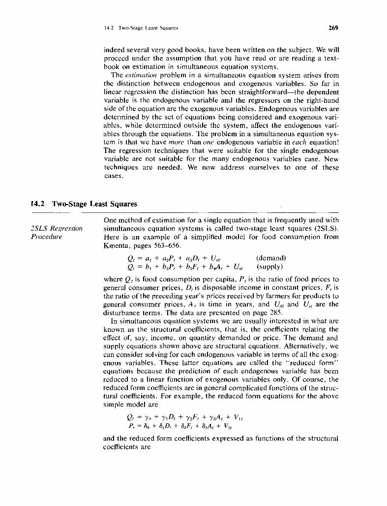
14.2 Two-Stage Least Squares 269
indeed several very good books, have been written on the subject. We willproceed under the assumption that you have read or are reading a textbook on estimation in simultaneous equation systems.
The estimation problem in a simultaneous equation system arises fromthe distinction between endogenous and exogenous variables. So far inlinear regression the distinction has been straightforward-the dependentvariable is the endogenous variable and the regressors on the right-handside of the equation are the exogenous variables. Endogenous variables aredetermined by the set of equations being considered and exogenous variables, while determined outside the system, affect the endogenous variables through the equations. The problem in a simultaneous equation system is that we have more than one endogenous variable in each equation!The regression techniques that were suitable for the single endogenousvariable are not suitable for the many endogenous variables case. Newtechniques are needed. We now address ourselves to one of thesecases.
14.2 Two-Stage Least Squares
2SLS RegressionProcedure
One method of estimation for a single equation that is frequently used withsimultaneous equation systems is called two-stage least squares (2SLS).Here is an example of a simplified model for food consumption fromKmenta, pages 563-656.
Qt = at + a2Pt + a3D f + Udf
Qt = ht + b2Pt + b3Ft + b4A t + Ust
(demand)(supply)
where Q t is food consumption per capita, P t is the ratio of food prices togeneral consumer prices, D t is disposable income in constant prices, F t isthe ratio of the preceding year's prices received by farmers for products togeneral consumer prices, A t is time in years, and U(lt and Ust are thedisturbance terms. The data are presented on page 285.
In simultaneous equation systems we are usually interested in what areknown as the structural coefficients, that is, the coefficients relating theeffect of, say, income, on quantity demanded or price. The demand andsupply equations shown above are structural equations. Alternatively, wecan consider solving for each endogenous variable in terms of all the exogenous variables. These latter equations are called the "reduced form"equations because the prediction of each endogenous variable has beenreduced to a linear function of exogenous variables only. Of course, thereduced form coefficients are in general complicated functions of the structural coefficients. For example, the reduced form equations for the abovesimple model are
Qt = Yo + ylDt + Y2F t + Y3A t + Vtf
Pt = 60 + 6tDt + 62Ft + 6:~At + V2t
and the reduced form coefficients expressed as functions of the structuralcoefficients are
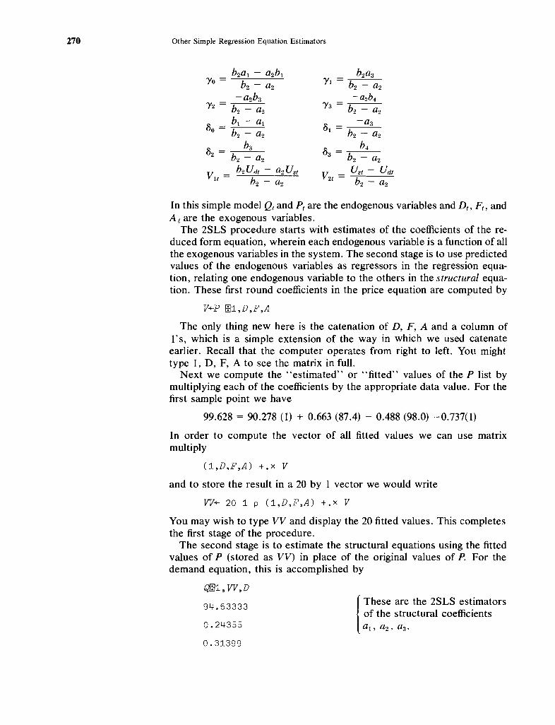
270 Other Simple Regression Equation Estimators
In this simple model Qt and Pt are the endogenous variables and Dt , Ft , andAt are the exogenous variables.
The 2SLS procedure starts with estimates of the coefficients of the reduced form equation, wherein each endogenous variable is a function of allthe exogenous variables in the system. The second stage is to use predictedvalues of the endogenous variables as regressors in the regression equation, relating one endogenous variable to the others in the structural equation. These first round coefficients in the price equation are computed by
V+-P ffi1,D,F,A
The only thing new here is the catenation of D, F, A and a column ofl's, which is a simple extension of the way in which we used catenateearlier. Recall that the computer operates from right to left. You mighttype 1, D, F, A to see the matrix in full.
Next we compute the "estimated" or "fitted" values of the P list bymultiplying each of the coefficients by the appropriate data value. For thefirst sample point we have
99.628 = 90.278 (1) + 0.663 (87.4) - 0.488 (98.0) -0.737(1)
In order to compute the vector of all fitted values we can use matrixmultiply
(1,D,F,A) +.x V
and to store the result in a 20 by 1 vector we would write
VV+ 20 1 p (1,D,F,A) +.x V
You may wish to type VV and display the 20 fitted values. This completesthe first stage of the procedure.
The second stage is to estimate the structural equations using the fittedvalues of P (stored as VV) in place of the original values of P. For thedemand equation, this is accomplished by
Qill1,VV,D
94.63333
0.24355
0.31399
{
These are the 2SLS estimatorsof the structural coefficientsat, a2, a3.

14.2 Two-Stage Least Squares
The structural equation is
Qt == 94.63333 - 0.2436 Pt + 0.3140 D t
Similarly, the supply equation is
QfE1, VV, F, A
271
or
49.53244
0.24007
0.25561
0.25292
{These are the 2SLS estimates of thestructural coefficients bI , b2 , b3 , b4 •
Qt == 49.53244 + 0.24007 P t + 0.25561 Ft + 0.25292 At
You may have noticed that the supply equation is exactly identified; thatis, the number of excluded exogenous variables from that equation is equalto the number of endogenous variables included in the regression as regressors. The excluded exogenous variable is D t and the included endogenousvariable is Pt.
In the exactly identified case we can derive estimates of the structuralcoefficients directly from the estimates of the coefficients of the reducedform equation. This is usually an exercise in algebra, where the values ofthe structural coefficients to be estimated are obtained by solving the equations relating the structural and reduced form coefficients in the exactlyidentified equation. To accomplish this we can estimate the reduced formequations for P and Q.
QI±J1,D,F,A Fffi1,D,F,A
71.20355 [The estimates of 90.26776{The estimates of the
0.15922the reduced form
0.66321 reduced form coeffi-coefficients Yo,
cients So, · . . , S3'0.13834 · · · , Y3' -0.48845
0.07598 -0.737039
Algebraically, we have
Q == 71.20355 + 0.15922D + 0.13834F + 0.075978A= B 1 + B2(90.26776 + O.66321D - O.48845F - O.737039A)
+ BsF + B~
After some algebraic manipulation we obtain
0.15922B2 = 0.66321 = 0.24007
B3 = 0.13834 - (0.24007)( -0.48845) == 0.2556
etc., which are in fact our 2SLS results. The other coefficients are left as an

272 Other Simple Regression Equation Estimators
exercise for the reader. It should be clear that even when the equations areexactly identified, 2SLS is a much simpler procedure than is indirect leastsquares. Of course, when the equation is overidentified (more excludedexogenous variables than included endogenous ones), you cannot use theindirect least-squares procedure, but you can use 2SLS.
As a final example, you may want to see what results you would haveobtained if you had performed ordinary least squares (O.L.S.) on thestructural equations. (Remember that these estimates are statistically inconsistent.)
The demand equation would be
QI131,P ,D
0.24355
0.31399
94.63333~The O.L.S. estimatesThe 2SLS estimates---?J'
99.89542
-0.31630
0.33464
and the supply equation would be
Ql±ll,P,F,A
58.27543
0.16037
0.24813
0.24830
~The O.L.S. estimatesThe 2SLS estimates~
49.53244
0.24007
0.25561
0.25292
The result of this section is that you can use APL to compute estimatesthat have desirable statistical properties. The procedures are not difficult.Even in the case of exactly identified equations, 2SLS using APL is easierthan the indirect least-squares approach. Two-stage least squares for thesystem we used requires two additional APL expressions over ordinaryleast squares, and that technique yields inconsistent estimates.
An alternative, but related, estimator that we will develop is the instrumental variable estimator. It is related to 2SLS in that the fitted valuesfrom the reduced form which we computed can serve as "instruments" forthe endogenous variables.
14.3 Instrumental Variables
InstrumentalVariables
In those situations in which the conditional distribution of the disturbanceterm is not independent of the regressors for whatever reason (some examples of this problem are "errors in variables" and simultaneous equationmodels), a useful approach to obtain estimators with desirable statisticalproperties is that of instrumental variables. More formally, but easier tounderstand, consider the model
y(N x 1)
X B +(N x K) (K x 1)
U(N x 1)

14.3 Instrumental Variables 273
where the dimensions of the arrays are given in parentheses below eacharray. The main difference between this model and that of Chapter 13 isthat here we assume that the distribution of the disturbance term U is notindependent of X, while in Chapter 13 we did assume such independence.
Now if (and it is a big IF), we can find another matrix Z of dimension(N x K) such that U is independent of Z and the columns of A havepositive coefficients of determination with the columns ofX, then Z is saidto be a matrix of instrumental variables for X. You might care to rememberthat the nonindependence ofX and U may be caused by only one column ofX, say X b in which case the variables X2, ••• , x". can ""serve as their owninstruments. "
Well, if we have an instrumental matrix Z, how do we use it? The easyway to do it is this: transform the regression Y = XB + U to
Z'Y = Z'XB + Z'U
and now carry out an ordinary least-squares regression of Z' Y on Z'Xwhere, with proper choice ofZ, Z'X, a (K x K) matrix, is nonsingular. Themathematical solution is
BE (the estimatcr of B) = (Z' X)-lZ' Y= B + (Z'X)-lZ'U
The corresponding covariance matrix of the regression coefficient estimators is defined by
(T:2(Z' X)-l(Z'Z)(X'2)-1
where fi2 is the variance of the disturbance term U. The required APLexpressions are
BE+((QZ)+.XY)~(ZX+(~Z)+.XX)
VARU+(+/(UH+(Y-X+.xBE»*2)7-/(pX)
COVBE+VARUx(ffiZX)+.x(~Z+.xZ)+.x~(QZX)
In order to illustrate the use of instrumental variables, we will write avery simple and straightforward routine to do the necessary calculations,but we'll omit all the frills that we put intoMREGRESS; these you can addlater. Consider
VBE+INSTRVAR
[lJ BE+((~Z)+.xY)~(ZX+(~Z)+.xX)
[2] VARU+( +/ (UH+( y- X+. xBE) )*2) 0;- - / (pX)
[3J COVBE+VARUx(WZX)+.x((~Z)+.xZ)+.xffi(~ZX)
[4J V
We will check the routine with some data cited by Kmenta, page 313.
y
0.768 0.433 0.4575 0.5002 0.3462 0.3068 0.3787 0.1188 0.1379

274 Other Simple Regression Equation Estimators
0.2001 0.3845
X
3.5459 3.2367 3.2865 3.3202 3.1585 3.1529 3.2101 2.6066
2.4872 2.428 2.318
z
3.4241 3.1748 3.1686 3.2989 3.1742 3.0492 3.1175 2.5681
2.5682 2.6364 2.5703
X+Q2 l1p ((11 pl),X)
X
1 3.5459
1 3.2367
1 3.2865
1 3.3202
1 3.1585
1 3.1529
1 3.2101
1 2.6066
1 2.4872
1 2.428
1 2.318
Z+ Q2 11p (( 11 p 1 ) , Z )
z
1 3.4241
1 3.17 Ll-8
1 3.1686
1 3.2989
1 3.1742
1 3.0492
1 3.1175
1 2.5681
1 2.5682
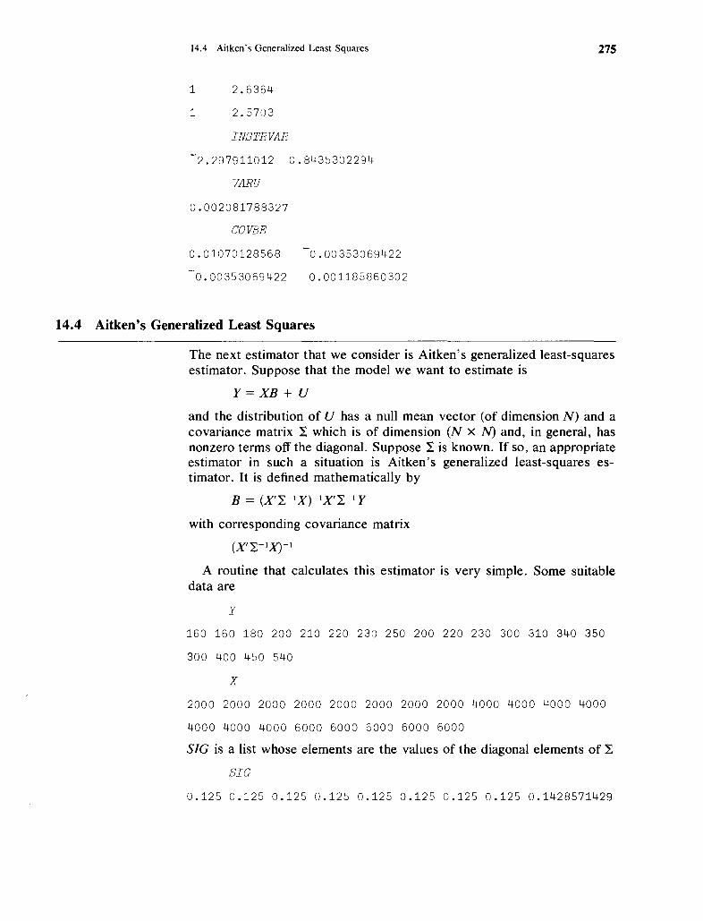
14.4 Aitken's Generalized Least Squares
1 2.6364
1 2.5703
INSTRVAR
2.297911012 0.8435302294
VARU
0.002081788327
COVBE
0.01070128568 -0.00353069422
0.00353069422 0.001185860302
14.4 Aitken's Generalized Least Squares
275
The next estimator that we consider is Aitken's generalized least-squaresestimator. Suppose that the model we want to estimate is
Y = XB + V
and the distribution of U has a null mean vector (of dimension N) and acovariance matrix I which is of dimension (N x N) and, in general, hasnonzero terms off the diagonaL Suppose I is known. If so, an appropriateestimator in such a situation is Aitken's generalized least-squares estimator. It is defined mathematically by
B = (X'L-1X)-lX'L-1Y
with corresponding covariance matrix
(X'L-1X)-1
A routine that calculates this estimator is very simple. Some suitabledata are
y
160 160 180 200 210 220 230 250 200 220 230 300 310 340 350
300 400 450 540
x2000 2000 2000 2000 2000 2000 2000 2000 4000 4000 4000 4000
4000 4000 4000 6000 6000 6000 6000 6000
SIG is a list whose elements are the values of the diagonal elements of L
SIG
0.125 0.125 0.125 0.125 0.125 0.125 0.125 0.125 0.1428571429

276 Other Simple Regression Equation Estimators
0.1428571429 0.1428571429 0.1428571429 0.1428571429
0.1428571429 0.1428571429 0.2 0.2 0.2 0.2 0.2
These data are from Kmenta, page 259.
Z+QZ~2 20 pZ~Y,X
z160 2000
160 2000
180 2000
200 2000
210 2000
220 2000
230 2000
250 2000
200 4000
220 4000
230 4000
300 4000
310 4000
340 4000
350 4000
300 6000
300 6000
400 6000
450 6000
540 6000
A useful routine for calculating Aitken's generalized least squares is
Aitken'sGeneralized LeastSquares [1J
VAITKNGLS[OJv
\jBE~Z AITKNGLS SIG
Y~Z[;1J
[2J X~Z[;(1(pZ)[2J-l)+lJ
[ 3] NN+-NxN+ p __SIC
[4J (N,N)p(NN pl,N pO)\SIG
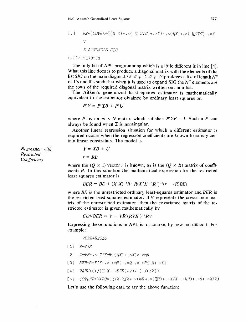
14.4 Aitken's Generalized Least Squares 277
Regression withRestrictedCoefficients
[5J BE~(COVBE+ill(Q X)+.x( ~ SIG)+.xX)+.x(~X)+.x( ffiSIG)+.xY
V
Z AITNKGLS SIC
0.07315178571
The only bit of APL programming which is a little different is in line [4].What this line does is to produce a diagonal matrix with the elements of thelist SIG on the main diagonaL (N N p 1,N po)produces a list of length N2of 1's and O's such that when it is used to expand SIG the N2 elements arethe rows of the required diagonal matrix written out in a list.
The Aitken's generalized least-squares estimator is mathematicallyequivalent to the estimator obtained by ordinary least squares on
p' y == p'XB + p' U
where p' is an N x N matrix which satisfies P''LP = I. Such a P canalways be found when L is nonsingular.
Another linear regression situation for which a different estimator isrequired occurs when the regression coefficients are known to satisfy certain linear constraints. The model is
Y == XB + U
r = RB
where the (Q x 1) vector r is known, as is the (Q x K) matrix of coefficients R. In this situation the mathematical expression for the restrictedleast squares estimator is
BER == BE + (X'X)-1R '[R(X'X)-lR 'J-1(r - (R)BE)
where BE is the unrestricted ordinary least-squares estimator and BER isthe restricted least-squares estimator. If V represents the covariance matrix of the unrestricted estimator, then the covariance matrix of the restricted estimator is given mathematically by
COVBER = V - VR'(RVR')-lRV
.Expressing these functions in APL is, of course, by now not difficult. Forexample:
VBER+-RESLS
[1J B+Yl±]X
[2J Q+ffiR+.x(XIX+ffi (~X)+.xX)x.x~R
[3J BER+B+XIX+.x (~R)+.xQ+.x (R2-R+.xB)
[4J VARU~(+/(Y-X+.xBER)*2)+ (-/(pX))
[5] COVBER+-VARUx( XIX-XIX+. xC QR + .. x ([lR) +. xXIX+. xQR) +. xR+. xX_TX)
Let's use the following data to try the above function:

278 Other Simple Regression Equation Estimators
y
100 106 107 120 110 116 123 133 137
x1 1 1
1 1.04 0.99
1 1.06 1.1
1 1.11 1.26
1 1.11 1.13
1 1.15 1.03
1 1.2 1.02
1 1.24 1.03
1 1.26 0.98
R
1 0 0
1 1 0
R2
1 0
RESLS
1 1 109.6135479
VARU
373.1395307
COVBER
2.651315829E-12
2.651315829E-12
O.OOOOOOOOOEO
3.976973744E-12
4.391241842E-12
1.077097056E-12
O.OOOOOOOOOEO
1.988486872E-12
3.666426234El
14.5 Durbin's Estimator in First Order Autoregressive Models
All of the estimators so far have been defined in terms of some lineartransformation of the regressand vector 1:- i.e., all the estimators have beenof the type
B = AY
where A is some suitable matrix of known constants.

14.5 Durbin's Estimator in First Order Autoregressive Models 279
First OrderAutoregressiveModel
We come now to some estimators which are no longer linear in this senseand which involve iterated solutions. The basic idea is that we start withsome reasonable idea for A, say A 0, and from that we get
BI = AOy
We use B I to calculate an A I, from which we get
B2 = AIY
and so on. Usually, it is convenient and statistically justified to stop afterobtainingB2. The iterated nature of such estimators is sometimes not clearfrom the formulas in the textbooks, especially when one can obtain B2 as afunction (through A 1) of A 0 and Y directly. Our first example of such aniterated estimator is in the context of a time series model.
The model we are considering is
Y = XB + V
where Y is (T x 1), Xis (T x K), B is (K x 1), and U is (T x 1). The modelis similar to our previous models except that the covariance matrix of U isgiven by:
1 P p2 pT-I
P 1 pT-2
V = (72 = (72L
pT-t pT-2 .... . . . . 1
where p is the autocorrelation parameter, -1 < p < 1; i.e., we are assuming that V t = pVt- 1 + e t , where et is normally distributed with zero meanand constant variance, and et, es for t =1= s are statistically independent.
There are several methods of estimating a model of this type when p isunknown. (Of course, if p is known, then Aitken's generalized leastsquares, which was discussed above, can be used.) One of the best methods is a procedure due to Durbin (see, for example, the discussion inJohnston*). The regression model can be transformed to
Yt = Yt-IP + XtB - Xt-IBp + E t
where Yt denotes the array Y with the first observation deleted, Yt- 1 denotes the array Y with the last observation deleted, X t is the X matrix withthe first row deleted, and X t - 1 is the X matrix with the last row deleted.E t is the error term. There are now only T - 1 observations. The regression is a two-step procedure.
First Step: Use ordinary least squares to get an estimate r for p inYt = Yt~tP + XtB - Xt-IB P + E t
Second Step: (i) Transform variables to get (Yt - rYt-l), (Xl - rXC- 1);
(ii) Use ordinary least squares on the transformed vari-
* J. Johnston, Econometric Methods. McGraw-Hill, New York, pp. 192-199. 2nd Ed., 1972.

280 Other Simple Regression Equation Estimators
abIes to get an estimate for B; i.e., use (Yr - r Yt - 1) ==(Xt - rXt-1)B + Eto
In terms of the APL programming of the routine, we need to obtain theHlagged" arrays .Yt - l , Xt-l, perform an ordinary least squares (OLS) regressions, transform variables, and do another OLS regression. Consider thefollowing effort:
\JBE+-Y AUTOREG X
YL+-( L1+( ( ( (p Y) -1) pi) !J 0 ) ) / Y {Initial lagging of variables inlines [1] to [4].
Y+ ( L2+( 0 , ( (p Y) -1) pi) ) / Y
K+2+ (p X) [ 2 ] x 2
XL+L1fX
X+L2fX
BE+.Yffi (YL!J «pYL) p1) !JXL,X) {First step regression, line [5].
R+-BE[ 1J
[lJ
[2J
[2.2J
[3J
[4J
[5J
[6J
[7J
[8J
[9J
Y+-(Y-RxYL)
X+- ( X-RxXL)
BE+.YffiX
{Transform variables, lines[6] to [8].
{Second step regression [9].
[ • 5] AX MATRIX IS ASSUMED TO BE WITHOUT CONST.
[10J \l
Let's try an example. In order to see the difference between the estimates, calculate .YffiX with the original variables. First of all, you might wishto check that (YL ~ ( (p YL) p 1») XL) X) gives the expected matrix. Let'sreuse some familiar data.
y
1 1.06 1.07 1.2 1.1 1.16 1.23 1.22 1.27
p y
9
X
1 1
2.04 0.99
1.06 1.1
1.11 1.26
1.11 1.13

14.5 Durbin's Estimator in First Order Autoregressive Models
1.15 1.03
1.2 1.02
1.13 1.03
1.26 0.98
p X
9 2
YL
1 1.06 1.07 1.2 1.1 1.16 1.23 1.33
Y
1 1.06 1.07 1.2 1.1 1.16 1.23 1.33 1.37
XL
1 1
1.04 0.99
1.06 1.1
1.11 1.26
1.11 1.13
1.15 1.03
1.2 1.02
1.24 1.03
L1
111 1 1 1 1 1 0
L2
011 1 1 1 111
(YL, ( (p YL) pl),XL,X)
1 1 1 1 1.04
1.06 1 1.04 0.99 1.06
1.07 1 1.06 1 ..1 1.11
1.2 1 1.11 1.26 1.11
1.1 1 1.11 1.13 1.15
1.16 1 1.15 1.03 1.2
1.23 1 1.2 1.02 1.24
0.99
1.1
1.26
1.26
1.03
1.02
1.03
281

282 Other Simple Regression Equation Estimators
The result from the routine A UTOREG is simple:
Y AUTOREG X
1.16889455 0.1677267818
14.6 k-Class Estimators in Simultaneous Equation Systems (OLS, 2 SLS, and LimitedInformation Maximum Likelihood)
k-Class Estimators The last estimator to be discussed in this chapter is in fact a class ofestimators-the "k" class estimators to be precise-which occur in theestimation of regression models embedded within a system of simultaneous equations. The linear regression model is now written in the form
Y(T x 1)
Yl G1
(T x M 1) (M l x 1)+ Xl B1 +
(T x K 1) (Kt x 1)U
(T x 1)
where the dimensions of the arrays are put in parentheses below the arrays. Because the variables Yand Yt arejointLy determined by a system ofsimultaneous equations, V is not statistically independent of Y 1. Y 1 isknown as the matrix of included endogenous variables this equation, X 1 isthe matrix of included exogenous variables, and X 2 is a (T x K 2) matrix ofthe exogenous variables which is called the matrix of excluded (from equation 1) exogenous variables. We will make the simplifying assumption thatK2 ~ M t . Let X == (Xt X 2 ) , a T x (K1 + K2 ) matrix.
With such a model, an entire class of estimators can be defined by thenormal equations as follows:
[ Y~Yt-kV~Vt Y~Xl] [ql(k)] == [Y~Y-kV;Y]X;Y1 X;X 1 B 1(k) X;Y
where VI == Yl - Y1 , Y1 == X(X'X)-lX; Y1 , and Gt(k), RICk) are the k-classestimators; for the algebraic details, see Kmenta, Goldberger, or anyintermediate level econometrics textbook. If k == 0, one has the OLSestimator; if k = 1, the two-stage least-squares estimator, and so on. Thevalue of k need not be a preassigned constant, but could be a solution to amaximization problem involving the random variables, as, for example, inthe case with the limited information maximum likelihood procedure.
In setting up a program to obtain k-class estimators, let's consider somechanges to the approach we have taken so far.
Let's assume that stored in the computer is a matrix Z of dimensionT x NV, where NV is the number of variables in the system of equationsto be analyzed. Alternatively, and equivalently in APL, the data could bestored as NV arrays of length T. The routine to be defined below will be aninteractive routine in that the routine, once it is called, will request inputfrom the user and process it accordingly.
The main steps in the calculation of the k-class estimators are:
(i) Fix the value of k and determine which columns ofZ are Y, Y 1J X h
and X 2 ;

14.6 k-Class Estimators in Simultaneous Equation Systems
(ii) Calculate V 1;
(iii) Set up the matrices appearing in the normal equations above;
(iv) Obtain the estimates GI(k), RI(k).
Consider the following routine:
V KCLASSEST;IND;Z;X2;Yl;VH1;Y;Q;P
[lJ 'ENTER NO. OF ARRAYS OF VARIABLES'
[2J NV+{]
283
[3J Ll+-L2+-L3+L4+NV pO
[ 4 J 'ENTER ARRAY NO. OF DEPENDENT VB L. '
[5J ND+-O
[6J Ll[NDJ+1
[ 7 J 'ENTER ARRAY NOS. OF ENDOGENOUS REGRESSOR VB LS.'
[8J NEND+-O
[gJ L2[NENDJ+l
[10 J 'ENTER ARRAY NOS. OF EXOGENOUS INCL REGRESSOR VB LS. '
[11J NEX+{]
[12J L3[NEXJ+1
[13J 'ENTER ARRAY NOS. OF EXOGENOUS EXCL. REGRESSOR VB LB.'
[14J NEXX+{]
[15J L4[NEXXJ+1
[16J L4[NEX]+1
[17J 'ENTER DATA ARRAYS' ;NV;' IN NO. '
[18J Z+{]
[19J VH1+Y1-X2+.x«Yl+L2/Z)~(X2+L4/Z))
[20J 'ENTER VALUE OF K FOR K-CLASS EST.'
[21J K+{]
[22J Y+-«(~Y1)+.x(Ll/Z))-Kx(~VH1)+.x(Ll/Z)),[lJ«~L3/Z)+.xLl/Z)
[23J Q+«(QY1)+.xYl)-Kx(C¥VH1)+.xVH1)~I2J«QY1)+.xL3/Z)
[24J P+«QL3/Z)+.xY1),[2J«QL3/Z)+.xL3/Z)
[25J BE+( ,Y)ffi(Q,[lJP)
[26J BE

284 Other Simple Regression Equation Estimators
Some discussion is needed for this routine, as it appears to be a littlecomplicated. However, the complications arise from only two sources: thedesire to pick out easily which arrays are to be the dependent variables,which the included endogenous, and so on; and the wish to define a wholeclass of estimators at once. To see how simple two-stage least squareswould be without the first requirement (having already removed the second), consider the following pair of lines:
YH1+X2+.x(YENDffiX2)
BE+YIIJ(YH1~X1)
where YEND is the matrix of included endogenous variables, X2 is thematrix of excluded exogenous variables, Y is the dependent variable array,and X 1 is the matrix of included exogenous regressors. This simple pair ofstatements generates 2SLS regression coefficient estimates if the appropriate arrays are already specified.
Let's return to the more conlplicated routine. The first step is to enterthe number of variables~ since we are going to extract Y, YI, Xl, and X2from Z by compression (Le., use of I). For example, L2 is an array (ofdimensionNV) of l's and O's-I's where the columns of Yl are located andO's elsewhere. The device NV~, used to solicit a response from the user,has been discussed previously.
In line [18] the user is prompted to insert data in the form of a matrix Z.You can do this by catenating the variable arrays which we have assumedare already stored in the computer. For example, if Q, P, R, S, Ware thearrays needed, you type (after the computer prompts with D)
where T is the numbers of observations. This action creates a matrix Zwhose columns are Q, P, etc.
Line [19] calculates VI. Lines [22J and [23], [24J define the arrays shownin the normal equations whose solution yields the required k-class regression coefficient estimates; this is done in line [25].
Line [22] is a straightforward programming version of the mathematicalstatement wherein the two parts of the Y array are catenated together.Lines [23], [24], and [25] are a little more tricky in that we need the extension of catenation called laminate, which we discussed in Chapter 12. Thetwo-dimensional array Q contains (Y{ Y1 - kV; V1 , Y;X1) , and P contains(X~ Y1 , X;X1), while(Q~[lJp)yieldsthe required matrix:
Line [25] raises another interesting little facet in APL. In the use of tildyadically, the left argument must be a list of length n if the right-handargument is a two-dimensional array of dimensions (n x q). The left argu-

14.6 k-Class Estimators in Simultaneous Equation Systems 285
ment must not be a two-dimensional array of dimensions (n x 1) or(1 x n). Thus, given the way in which the variable Y was created, (, Y)produces the appropriately dimensioned array.
To test our function, let us consider some data from Kmenta (pages 65365). The model, which we have used before, is
Qt = at + a2P t + a3Dt + Udt
Qt = hI + b2Pt + b3Ft + b~t + Ust
(Demand Equation)
(Supply Equation)
Here Qt is the quantity of food consumed per head per year, Pt is the ratioof food prices to general consumer prices, D t is disposable income, F t is theratio of the previous year's prices received by farmers to general prices,and At is time in years. Q and P are regarded as endogenous; D, F, and Aare exogenous. The demand equation is overidentified, and the supplyequation is exactly identified. The data are given in Table 14.1. These dataare simulated so that we know the true model, which is
Qt = 96.5 - 0.25 P t + 0.30 Dt + Udt
Qt = 62.5 + 0.15 P t + 0.20 Ft + 0.36 At + Ust
Let us use our k-class function with k == 0 (gives OLS) and k == 1 (gives2SLS). In this demand equation, P t is Y t and if = (1, 1, ... , 1), the D t areXl' and (Ft, At) are X 2 - We begin by entering the arrays Qt, Ph Dt, Fh and Atinto the computer.
The output is self-explanatory.
Table 14.1 Data List for Test of k-Class Estimators Routinea
Yor Qt(Dependent
Variable) Y1 or P t Xl or Dt X 2 or Ft X2 or At Xl or i
98.485 100.323 87.4 98 1 199.187 104.264 97.6 99.1 2 1
102.163 103.435 96.7 99.1 3 1101.504 104.506 98.2 98.1 4 1104.24 98.001 99.8 110.8 5 1103.243 99.456 100.5 108.2 6 1103.993 101.066 103.2 105.6 7 199.9 104.763 107.8 109.8 8 1
100.35 96.446 96.6 108.7 9 1102.82 91.228 88.9 100.6 10 195.435 93.085 75.1 81 11 192.424 98.801 76.9 68.6 12 194.535 102.908 84.6 70.9 13 198.757 98.756 90.6 81.4 14 1
105.797 95.119 103.1 102.3 15 1100.225 98.451 105.1 105 16 1103.522 86.498 96.4 110.5 17 199.929 104.016 104.4 92.5 18 1
105.223 105.769 110.7 89.3 19 1106.232 113.49 127.1 93 20 1
a These data are stored for us (the authors) in an array called K 565.

286 Other Simple Regression Equation Estimators
First round-Ordinary Least-Squares Estimators (K =0):
KCLASSEST
ENTER NO. OF ARRAYS OF VARIABLES
0:
6
ENTER ARRAY NO. OF DEPENDENT VEL.
D:
1
ENTER ARRAY NOS. OF ENDOGENOUS REGRESSOR VBLS.
0:
2
ENTER ARRAY NOS. OF EXOGENOUS INCL REGRESSOR VBLS.
0:
3 6
ENTER ARRAY NO/3. OF EXOGENOUS EXCL. REGRESSOR VBLS.
0:
4 5
ENTER DATA ARRAYS 6 IN NO.
0:
K565
ENTER VALUE OF K FOR K-CLASS EST.
0:
o
0.3162988049 0.3346355982 99.89542291
Second Round-2SLS Estimators (K == 1):
KCLASSEST
ENTER NO. OF ARRAYS OF VARIABLES
0:
6
ENTER ARRAY NO. OF DEPENDENT VEL.

14.6 k-Class Estimators in Simultaneous Equation Systems
0:
1
ENTER ARRAY NOS. OF ENDOGENOUS REGRESSOR VBLS.
0:
2
ENTER ARRAY NOS. OF EXOGENOUS INCL REGRESSOR VBLS.
0:
3 6
ENTER ARRAY NOS. OF EXOGENOUS EXCL. REGRESSOR VBLS.
0:
4 5
ENTER DATA ARRAYS 6 IN NO. 0
0:
K565
ENTER VALUE OF K FOR K-CLASS EST.
lJ:
287
1
0.2435565378 0.3139917943 94.63330387
Third Round-Limited Information Maximum Likelihood Estimators
(K = 1.1739):
KCLASSEST
ENTER NO. OF ARRAYS OF VARIABLES
0:
6
ENTER ARRAY NO. OF DEPENDENT VEL.
D:
1
ENTER ARRAY NOS. OF ENDOGENOUS REGRESSOR VBLS.
0:
2

288 Other Simple Regression Equation Estimators
ENTER ARRAY NOS. OF EXOGENOUS INCL REGRESSOR VBLS.
0:
3 6
ENTER ARRAY NOS. OF EXOGENOUS EXCL. REGRESSOR VBLS.
D:4 5
ENTER DATA ARRAYS 6 IN NO.
0:
K565
ENTER VALUE OF K FOR K-CLASS EST.
0:
.739
0.2295353985 0.3100126821 93.61902556
LimitedInformationMaximumLikelihoodEstimators
Summary
The value of k in the L.I.M.L. estimator is obtained by minimizing theratio of the error sum of squares of the regression of (Y - Y1G t ) on Xl andon X; for an explanation, see Kmenta (page 569).
We have now reached the end of the book. We trust that you havediscovered by this stage the power (and beauty) of APL and, more importantly, that in using APL you learned statistics more easily and fully thanwould otherwise have been possible.
There is more to learn, in APL statistics and econometrics. To dothat you will need to read some more books. As far as APL is concerned,you might now find it useful and interesting to look through some of thecomputer manuals recommended in the bibliography. The statistics andeconometrics books listed are all excellent at their various and respectivelevels of sophistication and detail.
This chapter discussed a number of APL routines for calculatingregression estimators in some interesting extensions to the simple model.The first topic is that of simultaneous equations. The program to estimatethe general k-class estimators was given. In addition, the 2SLS, indirectleast squares, and instrumental variables estimators were discussed atlength.
The next topic to be discussed was Aitken's generalized least-squaresprocedure, which is needed to estimate regression models where thecovariance matrix of the disturbance terms is nonscalar.
Another useful extension was to consider Durbin's method for estimat-
Exercises 289
Exercises
ing a linear regression model, where the disturbance term was distributedaccording to a first order autoregressive process.
Statistical Applications
1. Write in APL the following formulas useful in simultaneous equationsystems.
(a) Z = Lnxn ~ IKxK , where ® is the mathematical Kronecker product.
(b) B == [Z'(~-lQ9X(X'X)-lX')Z]-I[~-lQ9X(X'X)-lX']Y
(c) B == [Z[10X(X'X)-lX']Z]-lZ[1Q9X(X'X)-l]y
2. Let the true model be Y = 2X1 + 3X2 + Ut, where
0.2 0.10.3 0.80.4 0.60.5 0.50.6 0.50.7 0.4
The U t are identically and independently distributed random variables with mean zero and variance 1 (see the solution for a routinethat generates independent random numbers from a normal distribution with zero mean and variance equal to N(O, 1».
(a) Given X and U, find the values of 1':
(b) Compute the variance of Y using the computed values of 1':
3. Consider the follo't:ving data:
y Xl X2..~----_ ....-.~
49 35 5540 38 6046 40 7045 41 6152 42 6859 38 7155 31 5961 44 6664 38 7565 29 85
where Y == the production, in thousands of bushels, of wheat of onefarm over a period of 10 years; Xl = mean January temperature; andX2 = mean June temperature.Let the relationship between the variables be linear and of the formY = ao + atX1 + a2X2 + U.

the unconstrained vector of a.
the restricted vector of a.r == 0
290 Other Simple Regression Equation Estimators
Test the following hypotheses:
Ho: az = 0against H t : az * 0
andHo: ao = at = az = 0
against HI: ao, at, az '* 0
Use a 5% significance level for your tests.
4. Referring to exercise 3, suppose you believe that the June temperature affects the production twice as much as does the January temperature, and you want to test if your belief is true. Mathematically,this can be solved by the following steps (given without prooO.
(a) Find a = (X'X)-tX'y
(b) Find a == a + W(r - Ril)where R = [0 2 -I]
W == (X'X)-lR'AA == [R(X'X)-lR']-l Notice Ra == r ¢:> az == 2a1
(c) Find A= AR(il - ii) and V,," = u7,A, the variance-covariancematrix of A, where CT71 is the variance of the residuals from therestricted regression. * Thus under flo: az = 2a 1 A --- N(O, V~J,
which is equivalent to testing
H o: A = 0against Hi: A*-O
(d) Another statistic that you might want to use is
u'u ~ D'u n - k - 1a'a . s --- Fs,n-k-l
where li'u is the restricted error sum of squares, u'a is theunrestricted error sum of squares, and s is the number ofconstraints.
(e) Yet another statistic that you might want to use is
ii'a-21n ~
uu
which is distributed as chi-square with 5 degrees of freedom.
(0 Do you get the same answers using the three different tests?That is, do you accept or reject your hypotheses in all threetests?
5. Consider the following simple market model:
qS = 2 + P + U qd = 4 - p + v
where qS is quantity supplied, qd is quantity demanded, the equilibrium condition is qS = qd, and u --- N(O, 3) and v ~ N(O, I), where uand v are independent.
* A is the Lagrange multiplier of the minimization problem L = ulU + 2'A(Ra-r).

Exercises 291
(a) Find the expected equilibrium price.
(b) Suppose that the government initiates an inquiry whenever theequilibrium price is more than $1.50. Find the probability of having the government make an inquiry in this market.
6. Refer to exercise 3. Suppose you believe that there is no constantterm in that relationship, and you run the regression
Y = a1Xt + aZX 2 + U
(a) Find the error sum of squares of this regression and compare it toerror sum of squares of the regression in exercise 3.
(b) Suppose that instead of running the previous regression, youdecide to run
Y = at V + a2X2 + U*
where V is the residual vector of the regression of X t on X 2,
including a constant term. Use the same data to show that theestimate of a z is the same as that given by the regression of Y onX 2 •
7. Write a program that will calculate the following statistics in theheteroskedastic model, which is given by Y = XB + U, where thecovariance matrix of U is L, which is diagonal with unequal elementson the diagonal.
(a) B = (X'L- 1X)-lX'2:- 1 Y, the efficient estimator of the vector ofregression coefficients, where L is a diagonal matrix whose elements are known in advance.
(b) The t-statistics for the B estimates.
(c) Use the regression rOlltine you have just written together with thedata set ~~TT (Appendix E) to estimate the regression
Y = ao + atXt + aZPt + V
where Y is the KWHR of the 15 plants for the first year, X is the BTUof the 15 plants for the first year, and P t is the vector of prices that the15 plants paid during the first year. L is a diagonal matrix with thenumbers 1 to 15 on its diagonal; the numbers correspond to the size ofthe plant (1 for the smallest, 15 for the largest) measured by the totalKWHR produced during the first year.
8. Consider the following model that determines the equilibrium priceand quantity of a product.
D t == ao - alPt + a2 Yt + Ult
St = bo + blPt + U2t
where Dt = quantity demanded, endogenous; Pt == price of product,endogenous; St = quantity supplied, endogenous; YZt = disposableincome, exogenous; Dt == St, the equilibrium condition.Utt , UZt are each identically and independently distributed normal

292 Other Simple Regression Equation Estimators
variables with means zero, variances CTT and CT~, respectively, andcovariance (T 12.
(a) Solve for the reduced form.
(b) Is OLS an appropriate method of estimation for the reduced formcoefficients?
(c) Generate by computer a sample of observations on U tt , U2t and Yt
for 20 observations and compute values for D t , St, and Pt bysolving the equations after picking values for the coefficients. Useyour generated data to run OLS and 2SLS regressions on bothequations and comment on your results.
9. Consider the very simple income determination model:
Ct = ao + at Yt + U f
Yt = Ct + It
where Ct = aggregate consumption, It == Investment (exogenous),Yt == GNP, V t == stochastic disturbance.Use the data set MACRO in Appendix E.
(a) Estimate ao and at using OLS on equation (1).
(b) Write the reduced form equation for C, (using equations 1 & 2).
(c) Estimate Qo and at using OLS on the reduced form equation for C.
10. Consider the following product market model for the United States.Use the data set MACRO. See Appendix E. Can you estimate theseequations?
Ct ~ QtYt + Q2RLt-l + Ult
It == b i Yt + b2RLt- 1 + U2t
Yt == Ct + It
Check to see which, if any, of these equations are identified.
11. Using the money supply series in data set MACRO, estimate theparameters of the model:
MLt = ao + Q 1MLt- 1 + V t
12. A partial adjustment hypothesis could state that the target level of percapita consumption (Ci) is a linear function of income, Le.:
Cf = Q + bYt
Actual consumption is adjusted towards C* according to
Ct - Ct- 1 = y[ct - Ct- t ] + Ut,O < Y < I
which means that people adjust their consumption towards the desired level. However, the adjustment is not generally accomplished inone period (y < 1). Use the data in MACRO from 1950 to 1977 inAppendix E to test this hypothesis. On the basis of your estimated

Exercises 293
model predict consumption for the year 1978 and check your prediction with the actual 1978 value of consumption.
13. Suppose that you want to test Milton Friedman's permanent incomehypothesis. You first want to translate his hypothesis into mathematical formulas and test it on real data. The entire model might besummarized in the following two equations:
Ct = a + bYpt
YPt = yLf=o(l - y)iYt _ i
These equations can be combined to yield the following final equation:
C t = ay + bYYt + (1 - y)Ct - 1 + V t
Verify that this final equation is identical to the model in exercise 12after substitution of Cr and reinterpret the estimated coefficients.

Appendix A
The Computer: Where ItIs and How to GetAccess to It
A.I Account Number and Password
Account No. andPassword
294
In this brief appendix you will learn how to "log-on" to the computer.First, let's repeat that every computer center has its own administrativeprocedures for determining who call use the machine and what resourcesare allocated to those users. Some organizations make these arrangementsfor you, otherwise you go to the computer center to do it yourself. In anyevent, it's nothing to be overly concerned about. Typically, a form iscompleted and you are given an "account number" and a "password,"and sometimes a budget or time constraint. The account numbers areusually six or fewer digits, and the passwords are eight or fewer characters(either digits or letters). As an example, at Stanford the ~~account numbers" have two parts: a user number-J66 for the project, and a usergroup-El. The password was H0V. (To discourage poachers, a slang termfor people who specialize in using other people's accounts for their ownpurposes-such as playing space war----one should keep his or herpassword confidential.)
With this administrative chore done, you are ready to begin. First find anunoccupied computer terminaL The keyboard looks like any electrictypewriter, and in fact the letters are in the same position. The end of thisappendix contains diagrams of some typical keyboards-one for an IBM5120 minicomputer, an IBM-2741 terminal and a DEC-Writer II, and aHewlett-Packard-HP2541A-literally hundreds of others exist, althoughmost have the standard keyboard layout and features. In other respects,each terminal is slightly different; they hide the on-off switch in differentplaces, provide extra buttons, extra keys, lights, and even electronic whistles. None of these matters should worry you, but you must be sure thatthe terminal has the special APL characters. If your terminal does not havethese special symbols, it is probably called an ASCII (American Societyfor Coded Information Interchange) terminaL These terminals do not support the special character set of APL; however, all is not lost. The APL

Appendix 295
language allows you to use mnemonic codes in place of the special symbols. Look at the letter R; above it is the Greek letter rho, p. To representp you would type the mnemonic code .RO and the computer would understand it to be the symbol p. We have included a list of mnemonic codesused in APL in Appendix C. These vary somewhat from computer tocomputer, and you should check with your facility if you must use one ofthese ASCII terminals. You are now ready to start, and we presume thatyou are sitting in front of the terminal.
A.2 Log-on Procedure
Log-on Procedures
On the IBM-5120 minicomputer there is a white switch on the front controlpanel marked APL/BASIC; push it to the APL position and turn the redpower (on-off) switch on. That is all there is to it. When the machine warmsup, the TV screen will say CLEAR WE, meaning that you are ready to gowith a clear workspace-the electronic equivalent of a blank piece ofpaper. If you have a 5120 or similar microcomputer, you can skip to thelog-off section of this appendix.
Those of you who are operating in a time-sharing environment will haveto use a more complicated log-on procedure. On the 5120, which is a smalldesktop minicomputer, there is one user. On a big computer, hundreds ofusers are connected to the computer. These connections are done in one oftwo ways: via a direct wire from your terminal to the computer, or over thetelephone system. If you see a telephone by every terminal, you know howyour terminal is connected.
Unfortunately the log-on procedure varies from computer center tocomputer center. However, the procedures are usually not difficult to acquire. We suggest that if you are not provided with a log-on proceduresheet by the computer center, you make one up yourself until you haveeverything memorized. Believe us, one of the most frustrating parts ofprogramming is learning how to get programming access to the computer;once that is done, the rest is plain sailing. The problem here is that, as wementioned above, every center has its own ideas about how people shouldlog-on.
Nevertheless, to give you an idea as to what is involved, consider thefollowing procedure. Starting with the direct wire situation, you turn onthe terminal and type the symbol ), then your account number andpassword, and then press the "return" key. This button sends one line ofinformation to the computer. This could look like
)1984:ME
your account being number 1984 and your password ME. This password issometimes called a "LOCK." The computer will respond with somethinglike:
062* ]0:41:32 9/10/80 Von Mises
OPR: SYSTEM AVAILABLE TO 22:30
296 Appendix A The Computer: Where It Is and How to Get Access to It
CLEAR WS
Translating this into English, it means that you are using telephone linenumber 62 (called a "port" by computernics), the time is 10:41 and 32seconds A.M. on the tenth day of September, 1980, and the user's name isVon Mises. The operator indicates that the system will be available until10:30 tonight.
If, when you turned on your terminal, you could not type on it, or whenyou typed nothing happened, it might be that the terminal is in local mode.Look for a switch marked COM/LOC for communication and local. Itneeds to be in the COM mode to communicate with the computer. ClearWork Space means you are ready to begin.
If you connect to the computer via a telephone line, you have exactly thesame log-on procedure, with the additional task of calling the computer.The procedure is simple enough; first you activate a small box called amodem. Modem stands for Modulator Demodulator. This modem essentially takes the signals from your terminal and sends them over the telephone line, and then retranslates the signals from the computer to yourterminal.
These modems are of two basic types: one a Data-Phone and the otheran acoustic coupler. The Data-Phone is usually a Western Electric device;you simply pick up the telephone receiver, press the "talk" button, anddial the computer's telephone number after you get a dial tone. When thecomputer electronically answers the phone, you will hear a high pitchedtone that indicates that the computer is ready for you. You then press the"data" button.
The computer will typically send a brief message or just onecharacter-a - or a *. You can now "log-on" exactly as the direct-wiredterminal user does.
The final connecting device is the acoustic coupler. Again the terminalpower is turned on. With this equipment, the electric power to the modemis also turned on, and the telephone number is called. When you hear thehigh pitched tone, push the telephone hand set into the coupler receptacle.Sometimes there is an indication of which direction to place the hand set,but if there isn't, just take a guess. If it doesn't work, try it the other wayaround. Again, you will get some message from the computer and youlog-on.
As an exaplple, here is how it would be done at the Stanford ComputerFacility. OUf connection is hard wired, so we turn on the terminal (aGenCom, with the switch cleverly placed under the keyboard so that it isalmost impossible to find). I type an "a" and the computer responds with a+, I type SCF APL and the machine responds ... SCF 168 ... waits amoment and then types User? I type J66; it responds, Group? I tell it EI; itasks, Password? I reveal H0V (since changed) and it asks, Command? Irespond CALL APL; the machine types APL, then skips a line and typesCLEAR ws.
As another example, consider the sign-on procedure used at New YorkUniversity when using the CUNY computer center. At this point we runinto another option on terminals-some can be used for both APL and

Appendix 297
other languages. The character set for other languages is often designatedSTD CHAR SET (Standard Character Set), and you should be in standardto begin. The procedure is:
Switch on power of terminal and modem;
Ensure character switch is set to STD;
Dial up and place phone in acoustic coupler when high pitched tonecomes on line (a white light on the acoustic coupler comes on if theconnection is good);
Type "shift" P
Hit RETURN key (sometimes called EXECUTE);
System responds: type: a for apI, w for wylbur, 0 for callos
Type: a
Hit RETURN key;
System responds: PROJECT No., ID?
Type: [the project number given to you by the computer center];
System responds: PASSWORD?
Type: [the password you have picked and which is on file with thecomputer center];
Change character switch from STD to ALT;Type: )BLot [the '~)" symbol is upper case] key on the APL keyboard
(see end of this appendix)]
System responds: XXXXXXXXXXXXXXXXXXXXXXX
Type: ) followed by APL account number, the symbol: and password;
System responds:
Date Your Name [as filed in conlputer center]CUNY APL
Your log-on is now complete, and you are ready to begin.By now you realize that every center is different and will have its own
special way of logging you onto the machine. However, you now knowenough to understand the general idea of the log-on procedu.res used in anycomputer center. They all have handouts that explain the details and peculiarities of their own system.
A.3 Log-off Procedure
Logging off is simple. On the microcomputer systems you just turn themachine off. Of course, everything in the machine will be erased if you donot copy it onto a tape or disk. The same thing is true when you use theterminals. You must make special provision to save anything you want touse again. You learned how to do this in Chapter 7. If you have a 5120 orother microcomputer, you can skip to the last sentence of this appendix.

298 Appendix A The Computer: Where It Is and How to Get Access to It
To log-off on the terminal, you type )@FF and press the return button.The machine will respond, indicating that it understood your command.The response is something like:
062* 13:01:04Started 10:41:32
9/10/80 Von MisesClocktime this session 2:22:32CPUTime this session 0:00: 10
to date 17:25:30to date 00:01:10
Log-off Procedure
IBM 5120 desktopcomputer showing theAPL character set,numeric pad, andspecial function keys.
IBM 5120 showingkeyboard charactersthat can be enteredusing the command key
The first line here is similar to the first line of your terminal session; itindicates your port, the current time (1:04 P.M.), the date, and your name.The second line repeats the time you started and computes the elapsed
This top photograph showing a 5120 desktop computer can be programmedin either Basic or APL with the flip of a switch. The keyboard is exactly likea standard typewriter in that pressing the shift key (either of the keys withthe wide arrows on the bottom rank of keys) results in the APL charactersbeing entered into the computer. A convenient feature is that by holding thecommand key (CMD, on the far left) and pressing one of the keys on the toprow will produce an entire command. For example, holding down CMDand pressing I results in the command) LOAD being entered automatically.
The lower photograph shows the special overstruck characters that can beproduced with one stroke. The command is held down and any of theindividual keys now represents a new symbol or combination of key strokes.For example, pressing the CMD key and the F key results in the divide quador domino function being entered. If the machine were in the Basicprogramming mode the characters input would have been entered. Using theCMD key saves a number of key strokes and is a handy feature.

Appendix 299
Operator uses HewlettPackard 264lA CRTterminal specificallydesigned for APL andfeaturing extensivecommunicationscapabilities.
The operator IS using the H-P 2641A terminal as a device to communicatewith a central computer. In the upper right corner above the keyboard aretwo tape cassettes for data.
---- -_.-.r-;;:-- ,.; '-':;"-'
": ""'I-_.=~
[:~~~~J ...7 ....f! I:~:~2" -, ~1
... • ::: I.. ._-.J
Closeup of HewlettPackard 2641 A terminalkeyboard showing thevarious APL charactersand special functionkeys.
The closeup photo of the Hewlett-Packard 2641 A CRT terminal keyboardshows the APL characters, numeric pad, cursor control, and tape controlkeys. The dial in the upper left corner allows the operator to select thecommunications rate from 110 to 9600 band. The higher rates are used fordirect or hardwired communications to the host computer and the lowerrates are generally used when communication is over telephone lines.
time that you were connected to the machine for this session and all yourprevious sessions. The third line tells how much computer time you haveused.
The final steps are to disconnect the terminal from the computer andturn off the electricity to the equipment. If your terminal is hard wired orconnected via a DataPhone, just turn the electricity off. If the terminal is
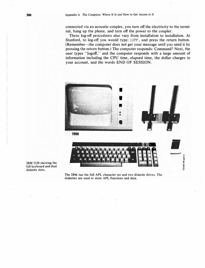
300 Appendix A The Computer: Where It Is and How to Get Access to It
connected via an acoustic coupler, you tum off the electricity to the terminal, hang up the phone, and tum off the power to the coupler.
These log-off procedures also vary from installation to installation. AtStanford, to log-off you would type: )OFF , and press the return button.(Remember-the computer does not get your message until you send it bypressing the return button.) The computer responds: Command? Next, theuser types "logoff," and the computer responds with a large amount ofinformation including the CPU time, elapsed time, the dollar charges toyour account, and the words END OF SESSION.
IBM 5120 showing thefull keyboard and dualdiskette slots.
The IBM nas the full APL character set and two diskette drives. Thediskettes are used to store APL functions and data.

Pictured is the MCMSystem 900 desktopAPL computer,manufactured by MCMComputers Ltd. ofKingston, Ontario,Canada and distributedin the United States byInteractive ComputerSystems, Inc., NewYork, New York.
Appendix
The MCM 900 is a desktop computer that can be programmed in APL as astandalone device. It can also be used as a communications terminal toother computers using its data communication interface. A number ofapplications routines are available to assist the APL programmer in theareas of business management, pension administration, bilingual wordprocessing, and financial accounting.
301

302
Appendix B
Longley Benchmark
The "Longley Benchmark," as it has come to be called, was developed ina paper titled" An Appraisal of the Least Squares Programs for the Elec-tronic Computer from the Point of View of the User." 1 The results wereshocking to some since a number of well-known and extensively usedprograms produced inaccurate results. In fact some of the computed coef-ficients have the wrong sign! Beaton and Barone used the same data in
OLS Regression EquationY = Bo + BIX} + B2X 2 + B 3X 3 + B4X 4 + BsXs + B¢f) + U
Regres-sand Regressor Variables
XlY GNP X5
Total Implicit X2 X4 NoninstitutionalDerived Price Gross X3 Size of Population 14Employ- Deflator National Unem- Armed Years of Age X 6
ment 1954 = 100 Product ployment Forces and Over Time
60,323 83.0 234,289 2,356 1,590 107,608 194761,122 88.5 259,426 2,325 1,456 108,632 194860,171 88.2 258,054 3,682 1,616 109,773 194961,187 89.5 284,599 3,351 1,650 110,929 195063,221 96.2 328,975 2,099 3,099 112,075 195163,639 98.1 346,999 1,932 3,594 113,270 195264,989 99.0 365,385 1,870 3,547 115,094 195363,761 100.0 363,112 3,578 3,350 116,219 195466,019 101.2 397,469 2,904 3,048 117,388 195567,857 104.6 419,180 2,822 2,857 118,734 195668,169 108.4 442,769 2,936 2,798 120,445 195766,513 110.8 444,546 4,681 2,637 121,950 195868,655 112.6 482,704 3,813 2,552 123,366 195969,564 114.2 502,601 3,931 2,514 125,368 196069,331 115.7 518,173 4,806 2,572 127,852 196170,551 116.9 554,894 4,007 2,827 130,081 1962
I Longley, James W., American Statistical Association Journal. Vol. 62, No. 31,7 September, 1967,pp. 819-841.

Appendix 303
other programs, and they found similar inaccuracies. 2 As a special check,they wrote their own routine, using multiple precision arithmetic and werecareful about the numerical analysis methods they used. Their results werein agreement with Longley's calculations. So we have some confidence inthe computed accuracy of the benchmark. We should add parentheticallythat Beaton and Barone caution researchers on interpreting regression results in problems of this nature. However, our point is that, ceterusparibus, more accuracy should be preferred to less.
We have included the raw data and some of the published results, andthe results from our APL runs with the l±I function.
Computed Coefficients
LongleyComputationUsing DeskCalculator
- 3482258.633015.061872271
-0.035819179- 2.020229803-1.033226867-0.051104105
1829.15146461
LongleyComputationUsing HighPrecision
Program 360
- 3482258.63459715.06187227161
-0.035819179293- 2.020229803818-1.033226867174-0.051104105653
1829.151461614112
APL-STAT
- 3,482,258 .63459493215.06187227114229
- 0.03581917929260994- 2.020229802817922-1.033226867173836- 0.05110410565236916
1829.151464613044
Standard Error of Regression Coefficient
Longley APL-STAT
890420.383684.91490.03350.48840.21430.2261455.4785
890420.386219183684.914925786191820.033491007837543010.48839968265023040.21427416335873260.2260732001756643455.4785004777639
Computed toO Values
Longley
- 3.91080.1774
-1.0695-4.1364-4.8220-0.2261
4.0159
APL-STAT
- 3.910802906682440.1773760282034131
-1.0695163151363-4.136427347486052-7.821985306012059-0.2260511445525611
4.015889800933297
This should give you an idea of our results compared to the benchmark.You might want to try this problem on your computer with the APL-STATroutines and also with other program packages.
2 Beaton, A., Rubin, D., and Barone, J., .... The Acceptability of Regression Solutions: Another Look atComputational Accuracy," Journal of the American Statistical Association, Vol. 71, No. 353, March,1976, pp. 158-168.

Appendix C
APL Character Set
Single-Strike Characters
APL Set ASCII Set Mnemonic Name
+ + addA-Z A-Z alphabetics
/\ & .AN ANd+ -E- or_ assignment
concatenate, commacolondecimal point
...- % .DV DiVide= equal to\ \ expand
* * exponentiate> > .GT Greater Than[ [ left bracket( ( left parenthesis< < .LT Less Thanx # multiply
0 .... 9 0-9 numerics,quote string
? ? question (roll and deal)/ reduce] right bracket) right parenthesis
semicolonsubtract
t 1\ .TK TaKe.US UnderScore
r .AB residue (ABsolute value)a .AL ALpha0 .BX quad (BoX)r .CE CEiling (maximum)
304

Appendix 305
Overstruck Characters
APL Set ASCII Set Mnemonics Name
¢ .RV ReVersal~ .TR TRanspose1. .XQ eXecutel' .PM ForMat
A-Z .ZA-.ZZ underscored alphabeticstl .Z@ underscored lower del
Single..Strike Characters
APL Set ASCII Set Mnemonic Name
{- .DA drop (Down Arrow).DD Dieresis
l. .DE DEcodeV $ .DL DeL·0 .DM DiaMondn .DU Down UnionT .EN ENcodeE .EP EPsilonL .FL FLoor;;::: .GE Greater than or Equal-+- .GO GO to (branch)1 .10 IOta{ .LB Left Brace~ .LD delta (Lower Del)~ .LE Less than or EqualI- .LK Left tacK0 .LO circle (Large 0)~ .LU Left Union~ .NE Not Equal to
.NG NeGation
.NT NoTw .OM OMegav .OR OR} .RB Right Brace--i .RK Right tacKp .RO RhOc .RU Right Union0 .SO jot (Small 0)U .DU Up Union
Overstruck Characters
APL Set ASCII Set Mnemonic Name
A LAmp (Comment)! factorial$ $ .DS dollar sign, .GD Grade Down~ .GU Grade UpI .IB I-Beame .LG LoGarithm'J'( .NN NaNdIt/' .NR NoR\ .CB Column expansione .CR Column Rotatef .CS Column Reduction[] .DQ Divide Quad0 .OU OUt'if .PD Protected Del

Overstruck Characters
NAME CHARACTER KEYS
Comment CD [J
Compress* f OJ CJExecute OJ [J
Expand* OJ CJFactorial, Combination CD 0Format OJ CDGrade Down CD rnGrade Up CD QJ
Logarithm ITJ (IJ
Matrix Division t}J rn CJNand '" (JJ Q
A
Nor v CD GJProtected Function v CD Q
Quad Quote [!J mGJRotate, Reverse
Q] (IJ
Rotate, Reverse* e(IJ CJ
Transpose Q OJ (IJ* These are variations of the symbols for these functions. These variations areused when the function is to act on the first coordinate of an array.
306
Appendix D
Saving Your Workspaceon The IBM 5110Microcomputer
If you want to save your workspace and you are using the 5120, you willuse the cartridge tape. You must first "mark" the number of tape files onthe tape and then transfer the workspace onto the tape. The details ofmarking the tape are not directly relevant for this discussion. However, ifyou type
)MARK 32 2 1
you will mark 2 tape files. The numbering of the files begins with one, andeach file contains 32 blocks of 1024 Bytes. There is enough room to store thewhole memory of a machine with 32,768 Bytes of core. The computer willrespond with
MARKED 0002 0032
To copy the workspace onto the tape, key in
)CONTINUE 1001 PROB
The first 1 indicates tape drive 1 (on the machine), 001 means you arestoring the information of the first file and you are naming it PROB. The5110 will respond
CONTINUED 1001 PROB
if all goes well. You could then take your tape out, turn the machine off andwalk away with the tape. Next time, after turning the machine on andobtaining the CLEAR WS signal, you would push the tape cartridge into themachine and key
)LOAD 1001 PROB
307
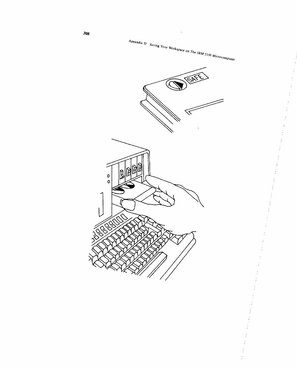
308
SaVing Your Workspace On The IE"" 5110 AI'
'VI 'Vl/crocOlllPuter

Appendix
The computer responds
LOADED 1001 FROB
309
and you are ready to go.The )SAVE , ) COpy , and )PCOPY commands are used in much the same
way as they were described in the previous section. If you skipped thatsection, you should read it now. The main differences concern marking thetape as you just learned, keeping track of the physical record number ofthe workspace, and the fact that continued workspaces are not automatically loaded when the computer is turned on.
If you forget the physical location (file number) of your saved workspaces, you can issue the )LIB command. The computer will respond withthe file number and the name of the workspace. It also displays otherinformation about the file-but that does not concern us now. Two warnings about this command are appropriate. Firstly, the computer does notautomatically rewind the tape to its beginning. You should issue the )REWIND command to accomplish this. Secondly, a small slot, marked withan arrow, exists on the top of the cartridge (see the figure). You must turnthe little wheel (a dime in the slot is perfect) until the arrow points awayfrom the word "safe," as in the figure. If the arrow points to "safe" thecomputer will not write on the tape, although you can read from the tape atall times.
On other mini- and microcomputers you may save your functions andvariables on floppy disks. This is also true for the IBM 5110 and 5120 seriesmachines. The procedure for disks is similar to the one we outlined fortapes.

Appendix E
Data Set 'Macro'A. GNP and its components Units of Measurement Abbreviations
1. GNP Billions of 1972 US $ y
2. Consumption Billions of 1972 US $ Ca) Nondurables Billions of 1972 US $ eNb) Durables Billions of 1972 US $ CD
3. Investment Billions of 1972 US $ I4. Government Billions of 1972 US $ G5. Imports Billions of 1972 US $ 1M6. Exports Billions of 1972 US $ X
B. Income1. Disposable Income Billions of 1972 US $ YD
c. Prices, Wages, Interest Rates1. GNP Deflator == 100 in 1972 P2. Short-term interest rates % per annum RS3. Long-term interest rates % per annum RL4. Wage rate in current US $' s W
per weekD. Employment
1. Employment Thousands of persons L2. Unemployment % U
E. Assets1. Capital Stock Billions of US $ K
F. Money Supply Billions of US $ MLSource: Economic report of the President, January 1979. Series only from 1950 to 1978.
Data Set Macro
Year y C I G X 1M YD
1950 533.5 338.1 93.7 97.7 21.7 17.7 205.51951 576.5 342.3 94.1 132.7 25.9 18.5 224.81952 598.5 350.9 83.2 159.5 24.9 20.0 236.41953 621.8 364.2 85.6 170.0 23.8 21.8 250.71954 613.7 370.9 83.4 154.9 25.3 20.8 255.71955 654.8 395.1 104.1 150.9 27.9 23.2 273.41956 668.8 406.3 102.9 152.4 32.3 25.0 291.31957 680.9 414.7 97.2 160.1 34.8 26.0 306.91958 679.5 419.0 87.7 169.3 30.7 27.2 317.11959 720.4 441.5 107.4 170.7 31.5 30.6 336.1
310

Appendix 311
Data Set Macro (Continued)
Year y C G X 1M YD
1960 736.8 453.0 105.4 172.9 35.8 30.3 349.41961 755.3 462.2 103.6 182.8 37.0 30.3 362.91962 799.1 482.9 117.4 193.1 39.6 33.9 383.91963 830.7 501.4 124.5 197.6 42.2 35.0 402.81964 874.4 528.7 132.1 202.7 47.8 36.9 437.01965 925.9 558.1 150.1 209.6 49.1 41.0 472.21966 981.0 586.1 161.3 229.3 51.6 47.3 510.41967 1,007.7 603.2 152.7 248.3 54.2 50.7 544.51968 1,051.8 633.4 159.5 259.2 58.5 58.9 588.11969 1,078.8 655.4 168.0 256.7 62.2 63.5 630.4
1970 1,075.3 668.9 154.7 250.2 67.1 65.7 685.91971 1,107.5 691.9 166.8 249.4 67.9 68.5 742.81972 1,171.1 733.0 188.3 253.1 72.7 75.9 801.31973 1,235.0 767.7 207.2 252.5 87.4 79.9 901.71974 1,217.8 760.7 183.6 257.7 93.0 77.1 984.61975 1,202.3 774.6 142.6 262.6 90.0 67.5 1,086.71976 1,271.0 819.4 173.4 262.8 95.9 80.5 1,184.41977 1,332.7 857.7 196.3 269.2 98.2 88.7 1,303.01978 1,385.1 891.2 210.1 275.2 107.3 98.7 1,451.2
Data Set Macro (Continued)
Year P RL RS W L
1950 53.64 2.62 1.45 53.13 58,9181951 57.27 2.86 2.16 57.86 59,9611952 58.00 2.96 2.33 60.65 60,2501953 58.88 3.20 2.52 63.76 61,1791954 59.69 2.90 1.58 64.52 60,1091955 60.98 3.06 2.18 67.72 62,1701956 62.90 3.36 3.31 70.74 63,7991957 65.02 3.89 3.81 73.33 64,0711958 66.06 3.79 2.46 75.08 63,0361959 67.52 4.38 3.CJ7 78.78 64,630
1960 68.67 4.41 3.85 80.67 65,7781961 69.28 4.35 2.97 82.60 65,7461962 70.55 4.33 3.26 85.91 66,7021963 71.59 4.26 3.55 88.46 67,7621964 72.71 4.40 3.97 91.33 69,3051965 74.32 4.49 4.38 95.45 71,0881966 76.76 5.13 5.55 98.82 72,8951967 79.02 5.51 5.10 101.84 74,3721968 82.57 6.18 5.90 107.73 75,9201969 86.72 7.03 7.83 114.61 77,902
1970 91.36 8.04 7.72 119.83 78,6271971 96.02 7.39 5.11 127.31 79,1201972 100.00 7.21 4.69 136.90 81,7021973 105.80 7.44 8.15 145.39 84,4091974 116.02 8.57 9.87 154.76 85,9351975 127.15 8.83 6.33 163.53 84,7831976 133.76 8.43 5.35 175.45 87,4851977 141.61 8.02 5.60 188.64 90,5461978 152.09 8.73 7.99 203.34 94,373
312 Appendix E Data Set 'Macro'
Data Set Macro (Continued)
Year U ML K
1950 5.3 0 01951 3.3 0 01952 3.0 0 01953 2.9 128.8 01954 5.5 132.3 01955 4.4 135.2 01956 4.1 136.9 01957 4.3 135.9 01958 6.8 141.1 01959 5.5 143.4 0
1960 5.5 144.2 01961 6.7 148.7 254.71962 5.5 150.9 269.71963 5.7 156.5 288.21%4 5.2 163.7 305.61965 4.5 171.4 336.01966 3.8 175.8 364.01967 3.8 187.4 386.21968 3.6 202.5 426.51969 3.5 209.0 473.6
1970 4.9 219.7 492.31971 5.9 234.0 529.61972 5.6 255.3 599.31973 4.9 270.5 697.81974 5.6 282.9 734.61975 8.5 295.2 756.31976 7.7 313.5 823.11977 7.0 338.5 900.11978 6.0 361.1 953.6
o Not available
Data Set Watt*List of the Plants
Number Plant Name
1 J. H. Cambell2 B. C. Cobb3 Dan E. Kern4 J. R. Whiting5 Rock River (Wis.)6 Nelson Dewey (Wis.)7 Minn. Power and Light Co., Clay Boswell8 81. Clair9 Presque Isle
10 Gulf Power (Scholtz)11 Gulf Power (Lansing Smith)12 Tampa Electric Company (P. J. Gannon)13 Northern States Power Co. (Lawrence)14 Montana Dakota Utilities Co. (Heshett)15 Appalachian Power Co., Clinch River
Source: U.S. Federal Power Commission, Steam Electric Plant Construction Cost and Annual Pro·duction Expenses 1966-1977.U. S. Energy Information Administration 1974.

Appendix 313
Data Set Watt
The data set WATT consists of three tables, the KWHR produced inTable 1, the BTU's used in Table 2, and the prices of BTU's in Table 3. Theobservations are for 15 plants over a period of 10 years. Thus, WATT is a 3by 10 by 16 (including the year column) three-dimensional array.
Table 1 Number of KWHR in millionsPlant Number
Year 2 3 4 5
1966 1,938.4 2,754.9 4,066.6 2,575.7 927.71967 2,980.4 2,752.4 3,878.5 2,425.5 977.81968 3,904.3 2,923.6 4,055.3 2,442.2 971.71969 3,678 2,907.9 3,900.7 2,393.9 987.91970 4,273.9 2,901.9 3,590.3 2,276.2 926.51971 3,316.7 3,244.4 3,558.2 2,190.1 807.51972 3,971.3 2,874.3 3,489.9 1,921.2 827.81973 4,103.7 3,449.8 3,438.2 2,211.8 862.41974 3,921.4 3,506.8 3,328.9 2,440.5 727.51975 3,460.9 2,869.6 3,032.5 2,155.4 546.9
Year 6 7 8 9 10
1966 1,393 892.2 9,792.8 854.2 246.01967 1,453.1 1,046.5 9,468.6 1,114.6 233.61968 1,505.9 1,023.2 9,373.4 1,135.4 313.41969 1,454.9 941.2 11,671.6 1,229.6 415.41970 1,275.0 947.9 12,620.4 1,161.4 389.41971 1,286.1 916.5 12,606.2 1,086.8 430.91972 1,439.8 945.6 12,386.8 1,121.0 433.31973 1,371.4 2,007.4 10,509.6 1,136.4 505.91974 1,126.5 2,773.6 9,958.2 1,130.8 462.21975 1,186.9 3,192.1 8,266.0 1,795.7 489
Year 11 12 13 14 15
1966 1,006.8 4,481.7 128 355.3 5,660.31967 1,648.4 4,666.5 176.2 462.5 5,345.61968 2,231.9 5,078.1 144.8 510.7 5,191.01969 2,173.2 4,954.9 113.2 497.7 5,353.91970 1,961.5 5,350.0 124.5 564.8 5,223.71971 1,754.6 4,736.7 133.3 583.2 5,052.41972 1,827.5 5,136.3 167.7 612.9 5,484.91973 2,043.8 4,880.3 168.1 575.9 5,575.21974 1,722.8 3,821.6 150.3 610.8 4,974.51975 1,592.3 4,392.5 40.8 602.9 4,202.2
Table 2 Number of BTU's in 1012 UnitsPLant Number
Year 2 3 4 5
1966 663.2 1,049.4 1,376.2 986.4 402.91967 1,093.6 1,066.4 1,331.9 942.3 413.91968 1,429.9 1,133.6 1,426.6 955 425.71969 1,349.5 1,138.9 1,384.6 955.2 440.51970 1,569.1 1,200.4 1,308.0 922 431.31971 1,237.8 1,363.0 1,302.6 913.1 378.11972 1,497.0 1,190.3 1,289.7 790.7 389.11973 1,540.4 1,424.3 1,282.9 831.3 414.21974 1,488.7 1,474.0 1,258.1 972 362.61975 1,355.4 1,238.1 1,128.8 838.4 291.4

314 Appendix E Data Set 'Macro'
Table 2 (Continued)
PLant Number
Year 6 7 8 9 10
1966 601 397.8 3,765.6 362.5 118.61967 625.6 426.9 3,633.5 454.2 110.21968 648.9 411.6 3,592.5 465.9 144.51969 631.6 485.5 4,483.7 507.6 192.51970 560.4 583.0 4,797.9 487.7 1861971 565.4 570.2 4,788.3 476.8 218.41972 638.1 605.8 4,508.5 511.5 224.31973 605.2 1,143.4 3,560.2 516.4 241.61974 507.2 1,707.6 473.9 549.4 2251975 600.8 2,063.0 2,434.0 794.3 235.5
PLant Number
Year 11 12 13 14 15
1966 422.1 1,965.5 18.3 330.2 2,069.51967 699.6 2,113.3 28.1 425.1 1,964.81968 941.5 2,340.2 16 467.3 1,912.51969 930.1 2,285.8 26.5 463.2 1,990.11970 868 2,466.3 31.8 520.2 1,972.01971 770.9 2,213.4 46.9 541.9 1,917.91972 849.0 2,420.6 52.6 571.3 2,068.51973 893.3 2,246.3 47.7 542.3 2,145.41974 771.3 1,808.1 59.6 575.9 1,948.61975 716.2 1,039.9 32.5 577.3 1,609.2
Table 3 Cost per Million BTU in ¢Plant Number
Year 2 3 4 5
1966 30.40 29.40 30.7 27.20 31.791967 27.30 29.90 31.80 27.70 32.381968 27.60 31.70 31.70 28.40 33.361969 29.00 34.00 31.80 30.10 34.941970 30.41 39.90 40.20 33.20 40.391971 34.10 45.50 46.60 41.60 47.801972 37.92 46.75 46.99 43.91 51.991973 44.00 49.20 48.34 61.43 55.491974 57.70 57.70 66.69 116.67 85.661975 111.90 101.30 104.9 142.40 133.90
PLant Number
Year 6 7 8 9 10
1966 26.78 35.54 28.30 32.44 30.011967 26.32 35.00 28.50 33.54 29.881%8 26.62 36.00 29.20 34.29 30.151969 28.41 36.00 29.40 35.96 31.961970 30.78 32.90 32.90 41.53 36.521971 34.11 31.70 39.70 51.30 43.701972 38.06 31.85 43.60 56.94 51.501973 43.37 31.68 47.71 64.10 54.801974 65.49 34.38 86.90 96.98 102.391975 96.60 62.00 106.00 134.03 136.83

Appendix 315
Table 3 (Continued)Plant Number
Year 11 12 13 14 15
1966 25.07 26.66 38.93 20.95 17.311967 25.29 26.13 38.18 20.52 17.711968 25.67 26.36 39.23 20.00 18.691969 26.99 29.28 41.45 20.42 20.361970 30.08 30.25 46.02 21.84 22.111971 40.02 31.02 54.09 22.90 26.471972 43.97 39.54 56.88 24.60 29.641973 46.74 49.80 65.51 25.36 34.501974 72.74 68.88 69.93 28.18 72.921975 124.40 123.00 135.95 45.50 128.90

Function Glossary
Table 1 Monadic Functions
Symbol Name Definition Example
+ Conjugate +A is A A
7
+A
7
Negative -A is a-A A
7
-A
7
x Signum xAis (A>Q) -A<O AWhen A is positive a 1results. When A is 7negative a 1 results.When A is zero a a xAresults.
1
x( -A)
1
Reciprocal f A is if A A
7
fA
0.14286
316

Function Glossary 317
Table 1 Monadic Functions (Continued)
Symbol Name Definition Example
Magnitude Absolute Value B
7.653 7.653 7.456 7.456
IB
7.653 7.653' 7.456 7.456
L Floor Least Integer B
7.653 7.653 7.456 7.456
LB
7 8 7 8
r Ceiling Greatest Integer B
7.653 7.653 7.456 7.456
fB
8 -7 8 7
7 Roll ?A is random number ?Afrom set of (p A)consecutive integers 1with each integerhaving the ( 1 +pA) 77777777probability of beingselected. 644 2 1 5 5
* Exponent eA A
7
*A
1096.6
Natural In A or logeA ALogarithm
7
f15.'A
1.9459
0 Pi Times 1TxA 01
3.1416
C
123
oC
3.1416 6.2832 9.4248

318 Function Glossary
Table 1 Monadic Functions (Continued)
Symbol Name Definition Example
Factorial !A=1 x 2x ... x(A-1)xA A
7
!A
5040
!4
24
Not ""1 is 0 , ""0 is 1. DTruth table defined foroand 1 only. 1 a 1
""D
0 1 0
f'oI ""'D
1 a 1
Table 2 Dyadic Scalar Functions
Symbol Name Definition Example
+ Plus Add 3 + 1.02
4.02
5 + 4
9
Minus Subtract 6 - 7
1
x Times Multiply 5 x 4
20
...- Divide Divide 5 ...- 4
1.25
Residue Remainder after divide 5125.010
0.01
L Minimum Smaller of two values 5 L 4
4
7.001 L 7.01

Function Glossary 319
Table 2 Dyadic Scalar Functions (Continued)
Symbol Name Definition Example
7.01
r Maximum Greater of two values 5 r 4
!1
7.001 r 7.01
7.001
* Power A to the B power: AB 3 * 2
9
4 * .5
2
~ General The base A logarithm of B 1ofA;) 5Logarithm
0.69897
10~1005
3.0022
Symbol Name
o Circular,Hyperbolic,andPythagoreanFunctions
Detinitlon
10X = Sine X
20X = Cosine X
30X = Tangent X
sox = SinhX
60X = CoshX
70X = Tanh X
-10X = Arcsin X
20X = Arccos X
- 30X = Arctan X
- SoX = Arsinh X
- 60X = Arcosh X
-70X = ArtanhX
OoX = (1+X*2)*.5

320 Function Glossary
Table 2 Dyadic Scalar Functions (Continued)
Symbol Name
BinomialCoefficients
Definition Example
The Bth term in the expansionof (X + Y)A, also the number ofcombinations of A things takenB at a time.
/\ And
v Or
'1< Nand (notand)
¥ Nor (not or)
A B A/\ E AvE A'l'<B A.¥ B
0 0 0 0 I I
0 1 0 1 1 0
1 0 0 1 1 0
1 1 1 1 0 0
A and B must be logical (0 or 1) variables
<:5
=
Less thanNot greaterthanEqual toNot lessthanGreater thanNot equal to
Result is 1 if relation holds (TRUE) andoif it does not hold (FALSE). For example,5 < 7 is 1, 5 > 7 is O.
Table 3 Dyadic Array Functions
Function
Plus
Symbol
+
Scalarf Array
3 + 4 8 2
7 11 1 587
Arrayf Array
3 4 1 + 246
Minus 3 - 4 8 2 3 4 1 - 2 4 6
15510 5
Times
Divide
Residue
Minimum
Maximum
x
L
r
3 x 482
12 24 6
3 -;. 482
0.75 0.375 1.5
314 8 -2
121
3L4 8 2
332
3r4 8 2
483
341x246
6 16 6
3 4 1 .;. 246
1.5 1 0.16667
3 4 112 4 6
200
3 4 1L2 4 6
241
3 4 lr2 4 6
346

Function Glossary
Table 3 Dyadic Array Functions (Continued)
Function Symbol Scalarf Array
321
Array f Array
Power
Logarithm
Circle
Binomial
And
Or
Nand
Nor
Less
Not greater
Equal
Not equal
Not less
Greater
*
o
v
<
=
>
3 * 482
81 6561 0.1111
3 fA} 4 8 2
1.2619 1.8928 0.63093
30 4 8 2
1.1578 6.7997 2.185
3 ! 482
4 56 0
1/\1010
1010
Iv1010
1111
1']\11010
0101
1"1'1010
0000
3<4 8 2 3
110 0
3--S4 8 2 3
110 1
3=4 8 2 3
a 001
3~4 8 2 3
1 110
32482 3
o 0 1 1
3 > 482 3
o 010
341 * 246
9 256 1
3 4 2 ~ 2 4 6
0.63093 1 2.585
3 410 2 4 0
2.185 4.1231 -0.27942
341 ! 246
016
10101\1100
1000
1010vl100
11101010'7'<1100
0111
1010;\/1100
0001
3 4 1<2 4 6
o a 1
3 4 1~2 4 6
011
341 = 246
010
3 4 1 ~ 246
101
3 4 1 2 2 4 6
110
3 4 1 > 246
100

322 Function Glossary
Table 4 Mixed Functions
ExamplesName Form Definition Arrays used in Examples:
Shape or pA Results in vector A B CSize whose elements
are the number of 1 2 3 10 20 100 200elements in A if Ais a vector, or the 4 5 6 30 40 300dimension of A ifA is an array. 7 8 9 50 60
70 80
pC
3
pA
3 3
pB
4 2
Ravel ,A Results in vector ,Awhose elementsare the elements 1 2 3 4 5 6 7 8 9ofA in row order.
Reshape ApE Reshapes the 2 2 pBravel ofB to shapespecified by A. 10 20
30 40
2 4 pA
1 2 3 4
5 6 7 8
3 5 pA
1 2 3 4 5
6 7 8 9 1
2 3 4 5 6
Reversal cPA or Reverses elements ¢AsA in A. ¢ reverses
the elements 3 2 1along the lastcoordinate. e 6 5 4reverses theelements along 9 8 7the firstcoordinate. eA
7 8 9
4 5 6

Function Glossary 323
Table 4 Mixed Functions (Continued)
ExamplesName Form Definition Arrays used in Examples:
1 2 3
<t>C
300 200 100
Rotate A¢B or The elements of 2¢CAeE B rotated A
positions. 1> 300 200 100rotates elementsalong the last 2¢Acoordinate and erotates elements 3 1 2along the firstcoordinate. 6 4 5
9 7 8
2eB
50 60
70 80
10 20
30 40
Trans- ~A or ~A transposes ~A
pose A~B the axes of arrayA.A~B, 1 4 7arranges axes ofBto conform to 2 5 8argument A.
3 6 9
~B
10 30 50 70
20 40 60 80
1 1¢A
1 5 9
2 1 ~A
1 4 7
2 5 8
3 6 9
1 2 ~A
1 2 3
4 5 6
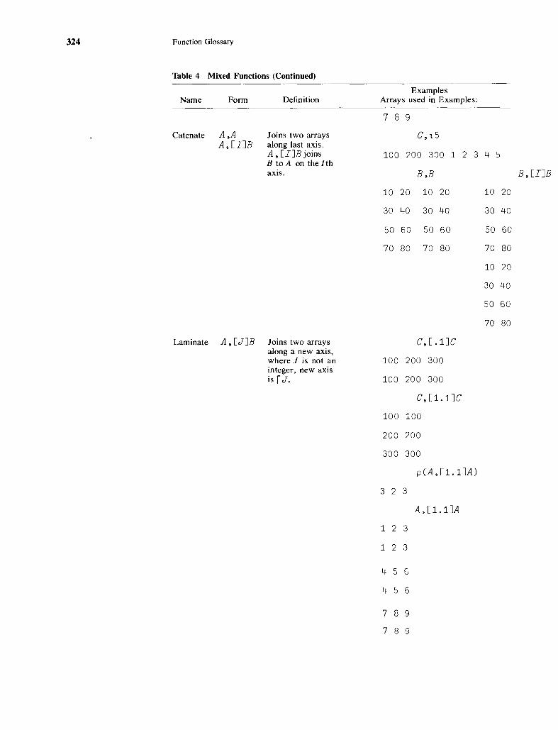
324 Function Glossary
Table 4 Mixed Functions (Continued)
Name Form
Catenate A ,AA, [IJB
Definition
Joins two arraysalong last axis.A , [IJB joinsB to A on the I thaxis.
ExamplesArrays used in Examples:
789
C,15
100 200 300 1 2 345
B,B B, [IJB
10 20 10 20 10 20
30 40 30 40 30 40
50 60 50 60 50 60
70 80 70 80 70 80
10 20
30 40
50 60
70 80
Laminate A , [J]B Joins two arraysalong a new axis,where J is not aninteger, new axisis rJ ..
C,C.1JC
100 200 300
100 200 300
C,Cl.1JC
100 100
200 200
300 300
p (A , C1 . 1 JA )
323
A, Cl.1JA
1 2 3
1 2 3
4 5 6
4 5 6
7 8 9
7 8 9

Function Glossary 325
Table 5 Mixed Functions
Name Form Definition Example
Take NtA IfN is positive, 2tC.first Nelements are 100 200taken and ifnegative, last 1tCN elements aretaken from 300vector A.
2 2tA
1 2
4 5
Drop N+A IfN is positive, 2+Cfirst Nelements are 300dropped and ifnegative, last 1iCN elements aredropped from 100 200vector A.
2 2+A
9
Compress N/A Selects 0 1 O/Celements fromA as deter- 200mined by zeroone argument 1 0 a/AN. For each 1in N, the cor- 1respondingelement in A is 4selected andfor each 0, the 7element is notselected. 1 0 O/[l]A
1 2 3
Expand N\A Fills array 1 a 1 1\Cwith alphabeticspaces or 100 0 200 300numeric zeroscorresponding 1 0 1 0 l\[l]Ato zeros in theargument N. 1 2 3
0 0 0
4 5 6
a 0 0
7 8 9

326 Function Glossary
Table 5 Mixed Functions (Continued)
Name Form Definition Example
Indexing A[ J Selects ele- e[l 3Jments from Adepending on 100 300expression en-
A[1;3Jclosed inbrackets.
3
A[1 2 3;3J
3 6 9
B[;2]
20 40 60 80
Index of A 1 B Returns the 1 2 3 4 5 6 717index value offirst OCCUf- 7rence ofB inA.
0 0 1 111
3
2 342 111 5 3
5 6 2
Index 1 A Generates first 110Generator A integers in
order. 1 2 3 4 5 6 7 8 9 10
Member- AEB Determines if 2 3 4 2 lE2ship each element
of A is a mem- 1 0 0 1 0ber of B.
2 3 4 2 lE2 3
1 1 0 1 0
Grade Returns the ~4 2 3 1 5Up index values of
A in ascending 4 2 3 1 5order.
A[M] Sorts the ele- Li 40 20 31 10 55ments ofvector A in 4 2 3 1 5ascendingorder. S[tiS+4 2 3 1 5J
1 2 31+5
Grade WA Returns the W4 2 3 1 5Down index of values
of A in 5 1 3 2 4descendingorder. t40 20 30 30 10 55

Function Glossary
Table 5 Mixed Functions (Continued)
327
Name Form Definition Example
A[tA] Sorts the elements ofvector A indescendingorder.
6 1 342 5
SCtS+40 20 30 30 10 55J
55 40 30 30 20 10
Deal A?B Selects A 2?20randomintegers with- 18 5out replace-ment fronl 1B , 10?10each integerhas a (1 +pB) 6 5 7 8 2 10 1 9 4 3chance ofselection. 10?10
10 9 4 3 6 8 5 2 1 7
Matrix fR4 Produces the RND+-2 2 p414Inverse inverse of a
nonsingular RNDmatrix.
1 3
4· 2
rIJRND
2 1.5
1 0.5
Domino B~ Domino can be 5X1
+ X2
+3X3
= 7used to solve aset of linear 10X
1+3X
2+SX
3 = 10equations if Ahas the same 2X
1+0. 2X
2+8. 3X
3=O
number ofrows as col- Aumns. Dominoreturns the 5 1 3coefficient ofleast-squares 10 3 5regression ifthe number of 2 0.2 8.3rows of Aexceeds the B+7 1 0 0number ofcolumns. BI±IA
1.7881 3.4851 0.51485

328 Function Glossary
Table 5 Mixed Functions (Continued)
Name
Domino fB
Quadoutput
Form
[frA
Definition
Displays A andgenerates a linefeed.
Example
AA
513
10 3 5
2 .2 8.3
2 3.5 0.5
B
71001
BlR4A forces interceptthrough zero
0.90461 0.20213 0.22486
BI±J1 !J AA catenate columnof ones for intercept
6.2918 0.26813 1.5607 0.7310
[fr' CHARACTER '
CHARACTER
[frSUMS++/B
18
Quotequadoutput
QuadInput
Quotequadinput
[!}+-A Displays Awith no linefeed.
A+{] Enters a line ofinput from afunction.
A+{!] Reads a line ofcharacters andcreates a character vectorfrom inside afunction.
In a Function
[!}+- , A1& & &' •
[!}+-'CHARACTER'
A 1 & & & CHARACTER
A+{]
D:
123
A
123
A+('J
A C B
A
A C B

Function Glossary
Table 5 Mixed Functions (Continued)
329
Name
Formatmonadic
Formatdyadic
Form Definition
"A Monadic formatA results in acharacter representation ofA so it can becatenated &displayed onsame line withcharacter data.
Al'B Displays Baccording tospecificationA. The firstelement ofA isthe number ofcolumns andthe second element is theprint precision.
Example
( 'THE LOG OF' ,"fA) , 'EQUALS' '-f~A
THE LOG OF 2 EQUALS 0.69315
A
5 1 3
10 3 5
2 0.2 8.3
2 3.5 0.5
6 3l"A
5.000 1.000 3.000
10.000 3.000 5.000
2.000 .200 8.300
2.000 3.500 .500
7 172 7 3"fA
5.0 1.00 3~000
10.0 3.00 5.000
2.0 .20 8.300
2.0 3.50 .500

330
Bibliography
Barron, D. W., Recursive Techniques in Programming, American Elsevier, NewYork, 196~
Beaton, A., Rubin, D., and Barone, J., fThe Acceptability ofRegression Solutions:Another Look at Computational Accuracy,' Journal of the American StatisticalAssociation, Vol. 71, No. 353, March 1976, pp. 158-168.
Dhrymes, Phoebus J., Distributed Lags: Problems of Estimation and Formulation,Holden-Day Inc., San Francisco, 1971.
Dhrymes, Phoebus J., Introductory Econometrics, Springer-Verlag: BerlinHeidleberg-New York, 1979.
Gilman, L., and Rose, A., APL An Interactive Approach, John Wiley and Sons,New York, 1976.
Hamburg, Morris, Statistical Analysis for Decision Making, Harcourt, Brace andWorld, Inc., New York, 1970, pp. 347-348.
IBM-APL Reference Manuals; APU360 User's Manual (GH20-0906), APL Primer(GH20-0689), APL Language (GC26-3847) IBM Corp., New York, 1977.
IBM 5110 APL Reference Manual, SA21-9303-1, IBM Corp., (General SystemDivision), Atlanta, 1978.
IBM Systems APL Language, GC26..3847-3, IBM Corp. (Programming Publishing),San Jose, 1978. .
Iverson, K. E.,A Programming Language, John Wiley and Sons, New York, 1962.
Johnston, J., Econometric Metlwds, McGraw Hill, New York, 1972.
Kaplan, W.,Advanced Calculus, Addison-Wesley, Boston, 1952.
Kmenta, J., Elements of Econometrics, MacMillan, New York, 1977.
Longley, James W., 'An Appraisal of the Least Squares Programs for the Electronic Computer from the Point of View of the User,' American StatisticalAssociation Journal, Vol. 62, No. 317, pp. 819-841, September 1967.
Mendenhall, W., and Reinmuth, J., Statistics for Management and Economics,Wadsworth, Belmont, California, 1978.
Bibliography 331
Neter, J ... Wasserman, W., Whitmore, G., Applied Statistics, Allyn and Bacon,Boston, 1978.
Pearson, E. S., and H. O. Hartley, Biometrika Tables for Statisticians, Vol. 1,Cambridge University Press, 1962, p. 104.
Press, James, Applied Multivariate Analysis, Holt, Rinehart and Winston: NewYork, 1972.
Rao, R. C., Linear Statistical Inference and Its Applications, John Wiley and Sons,New York, 1968.
Smillie, K. W., Stat Pac I, Department of Computing Service, University of Alberta, Edmonton, Alberta, Canada, 1968.
Smillie, K. W., Statpack2: an APL Statistical Package, Department of Computing Science, University of Alberta, Edmonton, Alberta, Canada, June1969.
Theil, H., Introduction to Econometrics, Prentice-Hall, New Jersey, 1978.
Wonnacott, T., and Wonnacott, R.,lntroductory Statisticsfor Business and Economics, John Wiley and Sons, New York, 1977.

Answers to Exercises
In this section a few answers to sel~cted problems are presented. Acomplete set of solutions to both the APL exercises and statistical problems is available from the publisher.
2 (f) Domain error
(k) 0 1 1.58 2
(p) Domain error
Statistical Applications (r) 2.5
1. 15.00 (u) 100
2. 13.33(v) 1 -1 2 -2
3. 91.1253. F1
-44 -18 0 6 10 12 124. 0.2457E-18 F3
5. (a) 254.97166 552 56 0 2 0 6 56
(b) 14.99 4. (a) 2
(c) 5.02 (b) 7 15
(d) 0.057656 (e) 1.83
6. 36,383.88 5. (a) 2.928
(d) 3085
(g) -5
3 (j) 110
7. (a) 45
APL Practice(e) 5.5
(h) 6.2£201. (a) blank (1) 82.999 82.5
(c) 0
(e) 3 Statistical Applications
(h) 3 1. a. 380.42. (a) 1 1 1 c. 1.0905
(d) 4 9 16 e. 0.08515
332

Answers to Exercises 333
2. a. 4.2
4. a.7.3%
b.0.8
6. a. $.8
b. 2.88 and 5.99
7. $194.32
4
4. c. 0.447
d. (1) 19.61, 20.51(2) 19.16, 20.95(3) 18.72, 21.40
5. d. 2
e. 0.6
f. zero
i. S3 = -0.6
S4 = 2.2
APL Practice 5
122J 2 2010
1. (0) (X[4X])[3]
2. (a) -2 -I -I 0 02 2 1 1 0o 1 0 1 0
(c) Same as Z
4. 3.246 3.246 -549
6. (a) X + 2X + 3X + 4X
(c) none
(d) I
8. The root is between 0.3169 and 0.3170
APL Practice
Statistical Applications
4. a. Mean = 2.6Variance = 3.3714Standard Deviation = 1.8361Mean Deviation = 1.64Median = 3
b. Mean = 3Variance = 6.2727Standard Deviation = 2.5045Mean Deviation = 1.9048Median = 3
5. a. weighted average = 2.044
8. a. 12.5
b. 159.17
1. (a) 0 0 0 0 0 0 0 0 0 0 0
(e) 6 7 8 9 0 1 2 3 4 5 6
(i) -3 -2(I) 0 0 -2 -1
(0) Index Error
2. (a) 3 random numbers from 1 to 6 withreplacement.
4. «7pO),4pl)/Z
5. We use the first 20 terms of each series.
(a) 0.69
(e) does not converge
(f) 0.58198
(i) =-.3
(k) does not converge
7. (a) Cauchy-Schwartz+ IX x Y s (+ /X*2) x (+ /Y*2)
8. (e) type--?'
(f) you will have an infinite loop.
Statistical Applications
2. The maximum value of S is 5 when P = .5and the minimum value of S is 0 whenP = 1.
3. Mean equals 5.920Variance equals 1.920Standard deviation equals 1.360

2. 0.8660.5000.5771.732
3. (b) \J CHECK [10][1] S~(L .5+ +/-7-(O,L50)!50) == 2\7CHECKYES
Statistical Applications
1. a. Nand M
e. 1 MNTS Xo2 MNTS X2.663 MNTS Xo4 MNTS X15.46
2. a. The sixth element of the series 10 bi .3is 0.1029.
d. 1-+15pl0BI .3 or 0.16
4. for P = .5 and K = 4 the probabilityf(N) = 0.0625
334
c. 124.95
d. 10.8
e. 750
9. 3.33, 0.68
6APL Practice
4. Problem
F<MF";?MF>M
5. 19.125
6. (a) 84(c) 2
7. 166.67
Answers to Exercises
Answer
('-F)/\MFv-MFI\-M
6. 2 POISSON 10.1839
12. Mean = 5Variance = 2.5Third moment == 0Fourth moment = 17.5Like the normal this distribution is bell
shaped but less peaked than the normal.
14. Mean == 6Variance = 2.4Third moment = -0.48Fourth moment = 16.224The distribution is skewed to the left
(since V 3 < 0).
15. a. 6 = 1/1008C
c. 0.055
h. 0.94
17. a. 0.6
d. 1.39
e. 6.11
7APL Practice
1. A (a) 1 2 3 4 5 6 7 8 9 10
(f) ABC DA B C D8
B (d) ABC DE F
(e) ABC DE FE F
2. (d) MEANThese data are for part D of Exercise
No.20:
(7*8,3) x (,10054, 921
5. )WSIDCLEAR WS
6. (b) (+/DATA) -7- pDATA
8. (d) 83325
tl. [3.5] --+ EXIT XL l=A/'FINISHED' ==
8pDISP

1. (a) 7 3.
12
(d) 1 YOU(e) WTACWTACWT 4.
WWWWWWWWWWTAC
2. They must be scalars
3. line [I] (+/X) not (+/x)7.
line [4] x +/(Y-MY) not x x/( Y -MY)
4. [3]~(N ~ PR)/2
7. Wo.rK
11. (c) [12.2][O]X TTEST Y; Nt; SS; XI; X2~NT; C; G;A;N2;NO
Answers to Exercises
Statistical Applications
2. a. -3.8696E-17b. -0.84543
3. a. 0.06 0.22 0.31 0.26 0.1 0.03 0.02
b..59 .41
4. TSX ~ NORM N[1] X (- ? (N,30)plO[2] SX ~ «(+/X)+ 30)- 5.5)+
(8.25+30)*.5 \l
8APL Practice
Statistical Applications
2. The result of ATTEST B is -1.15 andthe t-value from the t-table for 90%confidence is -1.812. Thus the programwas not effective.
3. 0.15
4. a. Computed poisson frequencies are223.13 334.7 251.02 125.5147.068 14.12 3.53 0.756430.14183 0.023683
5. a. $32.50
335
9APL Practice
1. (c) U~Y-A-BxX
(e) SU~S-+-(pX)-2
(k) VYXO~XUx«XO-XB)*2)+XSQ)++N
5. F(20) = !19F(3.5) = !2.5
Statistical Applications
1. a. R 2 = 0.043
d. R2 = 0.044
f. R2 = 0.036
Since F = .507 for the column meanswe are unable to establish a dependencyon dusting methods.
a. F for column means = 10.4, F(3,12) =3.49 so we reject hypothesis of nodifference.
Row means F = 2.3401Column means F = 0.045685Row & Col. means F = 1.4223
a) Ho not rejectedb) Ho not rejectedc) Ho not rejected.
10APL Practice
2. (a) 2 -5-1 3
(b) syntax error(c) 2 -1
-5 3(k) 123 78
44 28

336 Answers to Exercises
4. Left inverse is given by fE Z«~Z+.xZ)==(~Z)+.XQ~ Zresults in
1 11 1
6. 2.3 1-3.7 14.7 1
The rounding of the constants changed thesolutions dramatically.
8. a to g result in a matrix of ones provingthat the statements are true.
10. A=A+.xA andA==(~A)+.xA result inmatrices of ones.
12. 36.5 and 55.7
Statistical Applications
1. a. at = ¥-, lZ2 = t, var at = 1, var a2 = i2. i == 909.91, Y == 561.12,
Ii = -39.532, h == 0.66012
t == 69.824, R2 == 0.99449
3. a. x == 909.91, ij == 46.934,
Ii = -38.313, b == 0.093688
t == 32.659, R2 == 0.97531
b. i == 8.9271E5, Y == 46.934,
a == 2.4623, b == 4.9817£-5
t == 45.556, R2 == 0.98716
11APL Practice
4. (b) 1 1 1 0 1\[2]X
(c) 1 0 0 1 \ X
(d) 1, -1 44 jX
5. C~«0,L9)o.!0,t9)x 10 10 pI -1
then
(C+. x C)x (LI0) 0. == (LI0)gives a matrix of ones.
8. A~2 2pI 0 0 2
B~2 2p3 0 0 1
(AxB)=BxA
1 1
1 I
10. 1. +/[2]+/[3]ALL
2. r /[2]+/[3]ALL
3. +/+/+/ALL
Statistical Applications
1. Macro [;4] Regress Macro [;10]
i == 5.3714, Y == 135.76, a == 44.673,
h == 16.957,
t == 9.837, R2 == 0.78185.
2. Macro [;4] Regress Macro [;10]
after changing lines [4] and [5] to
[4] SSE~225x(n-2)
[5] V~225
:i == 5.3714, Y == 135.76,
Ii == 44.673, b == 1.8179,
t == 0.5126, R2 = 0.86654
12APL Practice
1. The required number is the mean of L
5. Q is a list of N random numbers from 1 toK
6. (a) (L 100) 0.* Ll0
(c) (LIOO) 0.*. t x LI0
(f) S~30 30p(.2*O,t29),.2 for p=.2
10. (a) 11.038
(b) 11.338, 11.15, 11.038, 11.225
13. (b) a row of ones
(c) you obtain c
(g) a matrix whose rows is either ones ornote.
Answers to Exercises
13Statistical Applications
1. a. Beta coefficients are 2.6706 and-129.42
their t ratios are 32.209 and -1.7648
3. Coefficients and corresponding t-ratiosa* at a 2
1.0223 0.42378 0.49806(0.027089) (18.425) (2.3033)
4. Coefficients and corresponding t-ratiosao at a2
2730.8 -1.5229 50.688(2.9563) (- 2.1977) (6.3059)
5. b. y = .9, b i = -.14, b2 = .37,bo = 57.67
7. t ratio for Ca = -1.99488. t- statistics
-2.3658, 51.987, 3.9462,-4.5486, 3.3161, 0.34169F == 25.888
9. a. F statistic == 5.1094 with 30 and 120degrees of freedom.
b. F statistic == 2.3604 with 30 and 120degrees of freedom.
10. ao == 7.7956 and a l == -0.32873Elasticity == - .32873
337
14Statistical Applications
3. t-statistic for a2 = 2.35 thus the H 0 isrejected.
F statistic == 197.7 and Ho is also rejected
5. a. equilibrium P == 1 & Q == 3.
6. b. ITest 1-0.23881, 0.79786, 0.79786
7. Beta coefficients == -569.26, 2.6626,19.659
t-ratios == -6.4608, 204.67, 7.0156
9. c. ao == 2.7769, at == 0.80121
11. ao == -10.298, at == 1.1005
coefficients t values12. l-y = 0.55511 5.9576
Yb == 0.30999 5.2282)'a == -22.376 -3.316
Using y 1978 == 1,385.1and C1977 == 857.7
we obtainC 1978 == -22.376 + .31(1,385.1)+ .56(857.7) == 883.11
which is close to the actual value of 891.2.

AAbsolute value 35-36~ 49, 62, 67Account no. 294Addition 7, 12Addressable cursor 25Administrative procedures 1Aitken's generalized least squares 275And 79APL program for linear regression 145APL keyboard 2, 298-301Arithmetic functions 6--10, 12Arithmetic mean 20~ 28Arrays 10-12, 172Arrays: parity 36Assignment 17, 28
BBarone, J. 303Barron, J. 76BASIC 7Basic statistics 58Beaton, R. D. 303Benchmarks 302Bibliography 330Binomial coefficients 73Binomial distribution 75Binomial probability 74Blanks 10, 12, 28Branching 45, 50Breaking up the sum of squares 145
CCase study in program develop-
ment 127Catenate 40, 49, 210Cathod ray tube 25Ceiling 62 ~ 67Character arrays 78, 98Character input 103Character set 304Checking parentheses 24Checking results 132Chi-square 148, 153Chi-square distribution 149Clear WS 2Column vector 172Combination of R things N at a time 74Command key 7Comment 163Compression 79, 81, 197Computers Ltd. 301Concave functions 92Conditional branches 45, 46, 50Contingency tables 149Contingency table routine 153Continuation 27, 29, 101Convex functions 92Correcting a defined function 47Correcting a function line 60Correcting typing 25, 42Correlation matrices 240Covariance 73, 240
338
Index
Covariance and correlation mat-rices 240
Cross products 72Cumulative Chi-square 161Cumulative F distribution routine 162Cumulative Poisson distribution 76Cursor 25
DData and information 97Data set ·Macro' 310Deal 43Debugging 127Del 41,50Deleting a line in a function 119Determinant 231Determinant routine 234Diagnostics 121Digital Equipment Corporation 294Display 48, 51Display numeric and character data on
one line 99
Display one or several lines of afunction 117
Distributions 73Divide 9, 12Domain error 9, 98Domino "180Drop function 214Dummy variables 63,67Durbin-Watson statistic 261Durbin's estimator in first order autore-
gressive models 278Dyadic compression 82, 197Dyadic expand 199Dyadic functions 16, 28Dyadic reshape 78
Ee 22
Elementary linear regression 144Elementary matrix operations 174Elementary statistics 15Entering data inside a function 101Entering data on two lines 27 ~ 29Entering function definition mode 41 ,
50Equal 79Estimators of regression coefficient 144Estimators of the variance of regression
estimators 144Execute 6-8, 18, 27Execution mode 2Exit from function 47Expand 193, 199Exponential function 22, 28
FFactorial function 74Features of APL 2First order autoregressive model 279Floor 62,67Format 100
F~Statistic 154Functions and arrays 11, 12Function definition 41, 50Function display 117Function glossary 316Function headers 43, 50
GGamma function 160Generalized least squares 275Generating random numbers 43, 49Getting started 6Geometric distribution 93Geometeric mean 21, 28Global variables 63, 67, 135Goodness of fit 148Grade down 38-39, 49Grade up 38, 49Greater than 79Greater than or equal to 79
HHamburg, M. 128Harmonic mean 23,28Heteroskedastic models 259Hewlett-Packard 294, 299Higher and cross product nloments and
distributions 72Higher-order arrays 191Higher order sample moments 72Histograms 76How mistakes begin 129How to calculate a mean 19, 28How to write your own function 34
IIBM I, 6, 294, 307, 234-235, 298, 307Identity matrix 179Immediate execution mode 2Index error 38Index generator 46, 49Indexing arrays 37,49, 193Inner product 27, 29, 22 IInner product generalized 222Input continuation 101Insert a new line 118Interactive programming 44Introduction to linear regression 144Instrumental variables 272Invalid variable names 18, 28Inverse 179Inverse of a nonsquare matrix 182
JJohnston, J. 268, 279
KKaplan, W. 161K·Class estimators 282Keyboard 2, 295, 298-301Keying conventions 6Kmenta, J. 26, 268, 269, 276, 285, 288

Index
Kronecker product 229Kurtosis 94
LLabel 45Lagged variables 259Lagrange multiplier 290Laminate 212Left inverse of a nonsquare matrix 181Length error 12, 98Less than 79Less than or equal to 79Limited information maximum likelihood
estimators 288Linear regression 183, 240Line continuation 27, 29Line labels 45, 50Local variables 65, 67Logarithm function 22, 28Logic of residue function 36Logical functions 79Log-Off procedure 297Log~On procedure 1, 295Longley benchmark 302Longley, J. W. 302Looping 232Lost results 18
MMacro, data set 310Making a program interactive 103Matrices 172Matrix addition 175Matrix algebra 172Matrix inverse 179Matrix multiplication 176Matrix subtraction 175Matrix transpose 178Maximum 77Maximum likelihood estimator 288MCM System 900 201Mean 19,28Mean and variance of probabilities 27,
29Median routine 58Minimum 77Minus 8, 12Mistakes, how they begin 129Modem 296Moment 240Monadic format 100Monadic function headers 44, 50Monadic functions 16, 28Multiline data input 101Multiply 9, 12
NNegative numbers 8, 12New line, insert 118Niladic function 41, 50Non-singular matrices 179Normal distribution 83Not and 79Not equal to 79
-Not or 79Numeric arrays 97Numeric input 102
oOne-way analysis of variance 154One-way anova 154OR 79Ordering arrays 37, 49Outer product 131, 152, 221, 223Overstruck characters 306Overview of APL 1
p
Parentheses 23Partial correlation coefficients 246Password 294Pearson, E. S. 87Pendent functions 126PI times 84Poisson distribution 75Power 22Private library 109Problems from careless use of global
variable 135Procedures, administrativeProduction functions 225Program development 127Program errors 127
QQuad 27,29Quad-divide 180Quad-input 102Quote 44, 50Quote-quad input 103
RRandom numbers 43,49Rank error 46Ravel 57, 66, 173, 209Reciprocal 17, 28Recursive programming 76Reduction 19, 28, 191Regression routine 146, 254Regression with restricted
coefficients 277Removing a suspended function 48, 51Reshape 173, 151Residual routine 148Residue 34-35, 49Restricted coefficients 277Return 6-- 10, 27Reverse or rotate function 200Rho 20,28Right inverse of a nonsquare matrix 182Right to left order 15, 28Roll 42, 49Rotate 200Row vector 172
SSampl~ median 34, 49
339
Sample results of regression rou-tine 147
Sample standard deviation 24, 29Sample variance 23, 29Saving workspace 106Saving workspaces on microcom-
puter IIISaving your workspace 307Scan 21,28Shape 20,28
SI Damage 48,51, 104, 126Simple and partial correlation
coefficients 245Simple least squares regression 144Simpson's rule 91Simultaneous equation models 268Singular matrices 179Smillie, K. W. 76Sorting an array 39Standard deviation 24, 29.. Standard" -normal density
function 84State diagram 2-3Statements automatically renum-
bered 119Standard deviation routine 58Stop 125Student's t 128Student's t test routine 135Subtraction 8, 12Sum of squares 145Suspended functions 126Syntax error 8, 12, 17System commands 18, 28System of linear equations 183
TTake function 213Terminating input request 103Trace 123, 136Transformed variables 258
, Trapezoidal rule 91Transpose 205Truth table 79Two-way analysis of variance 156Two-wayanova 156Two-way classification 150Two-stage least squares 269
UUnconditional branch 45, 50Using APL in the calculator mode 132
VValid variable names 18, 28Value error 64, 67Variables and assignment 17, 28Variable names 18, 28Variance 23, 29, 58Vectors 172Vectors matrices, and arrays 172
wWork space 2

Symbol Index
)OFF 2 I 62, 67; 77+ 7, 12 0 84
8, 12 99x 9, 12 l' 100
...- 9, 12, 28 +- D 102)VARS 18-19, 28 +- [!] 103/ 19, 28; 79; 191 )CONTINUE 106p 20, 28; 78; 151; 173 )WSID 107\ 20, 28; 193 )SAVE 107e9 22,28 )LOAD 107
* 22,28 )LIB 108+.x 27, 29; 121 )SA VE CONTINUE 108,0 27, 29; 101 )COpy 108I 34-36, 49; 62, 67 )PCOpy 108~ 38,49 )DROP 109t 38-39, 49 )FNS 110
40, 49; 57, 66; 173; 209; 0 117212 T~ 123
v 41,50 Sf1 125) CLEAR 42, 51, 109 )SIV 127? 43 0 131
44,50 o.x 152-+- 45,50 [lJ 1801 46,49 ¢ 2000 48,51 Cs? 205)ERASE 48, 51, 60, 109 t 213)SI 48, 51; 104; 126 + 214L 62, 67; 77
340
Related Documents
![[Preservation Tips & Tools] Section 106, Part Two: How You Can Get Involved](https://static.cupdf.com/doc/110x72/554a8476b4c90579288b5752/preservation-tips-tools-section-106-part-two-how-you-can-get-involved.jpg)