Dense Matrix Algorithms Ananth Grama, Anshul Gupta, George Karypis, and Vipin Kumar To accompany the text “Introduction to Parallel Computing”, Addison Wesley, 2003.

Welcome message from author
This document is posted to help you gain knowledge. Please leave a comment to let me know what you think about it! Share it to your friends and learn new things together.
Transcript

Dense Matrix Algorithms
Ananth Grama, Anshul Gupta, George Karypis, and Vipin Kumar
To accompany the text “Introduction to Parallel Computing”,Addison Wesley, 2003.

Topic Overview
• Matrix-Vector Multiplication
• Matrix-Matrix Multiplication
• Solving a System of Linear Equations
– Typeset by FoilTEX – 1

Matix Algorithms: Introduction
• Due to their regular structure, parallel computations involvingmatrices and vectors readily lend themselves to data-decomposition.
• Typical algorithms rely on input, output, or intermediate datadecomposition.
• Most algorithms use one- and two-dimensional block, cyclic,and block-cyclic partitionings.
– Typeset by FoilTEX – 2
Matrix-Vector Multiplication
• We aim to multiply a dense n × n matrix A with an n × 1 vectorx to yield the n × 1 result vector y.
• The serial algorithm requires n2 multiplications and additions.
W = n2. (1)
– Typeset by FoilTEX – 3

Matrix-Vector Multiplication: Rowwise 1-D Partitioning
• The n × n matrix is partitioned among n processors, with eachprocessor storing complete row of the matrix.
• The n × 1 vector x is distributed such that each process ownsone of its elements.
– Typeset by FoilTEX – 4

Matrix-Vector Multiplication: Rowwise 1-D Partitioning
1
p-1
0 1 p-1
0 1 p-1
0 1 p-1
0 1 p-1
0
1
p-10 1 p-1
p-1
p-1
.
.P
P
P
1
0
.
.
P
P
P
1
0
0
1
p-1
n/p
the processes by all-to-all broadcast
n
0
(d) Final distribution of the matrix and the result vector
(c) Entire vector distributed to each
p-1
.
.
P
P
P
0
1
.
.
P
P
P
0
1
p-1
(a) Initial partitioning of the matrix and the starting vector
Matrix Vector
VectorMatrix A x
yA
x
y
(b) Distribution of the full vector among all
Processes
process after the broadcast
Multiplication of an n × n matrix with an n × 1 vector usingrowwise block 1-D partitioning. For the one-row-per-process
case, p = n.
– Typeset by FoilTEX – 5

Matrix-Vector Multiplication: Rowwise 1-D Partitioning
• Since each process starts with only one element of x, an all-to-all broadcast is required to distribute all the elements to all theprocesses.
• Process Pi now computes y[i] = Σn−1j=0 (A[i, j] × x[j]).
• The all-to-all broadcast and the computation of y[i] both taketime Θ(n). Therefore, the parallel time is Θ(n).
– Typeset by FoilTEX – 6

Matrix-Vector Multiplication: Rowwise 1-D Partitioning
• Consider now the case when p < n and we use block 1Dpartitioning.
• Each process initially stores n/p complete rows of the matrix anda portion of the vector of size n/p.
• The all-to-all broadcast takes place among p processes andinvolves messages of size n/p.
• This is followed by n/p local dot products.
• Thus, the parallel run time of this procedure is
TP =n2
p+ ts log p + twn. (2)
This is cost-optimal.
– Typeset by FoilTEX – 7

Matrix-Vector Multiplication: Rowwise 1-D Partitioning
Scalability Analysis:
• We know that To = pTP − W , therefore, we have,
To = tsp log p + twnp. (3)
• For isoefficiency, we have W = KTo, where K = E/(1 − E) fordesired efficiency E.
• From this, we have W = O(p2) (from the tw term).
• There is also a bound on isoefficiency because of concurrency.In this case, p < n, therefore, W = n2 = Ω(p2).
• Overall isoefficiency is W = O(p2).
– Typeset by FoilTEX – 8
Matrix-Vector Multiplication: 2-D Partitioning
• The n × n matrix is partitioned among n2 processors such thateach processor owns a single element.
• The n × 1 vector x is distributed only in the last column of nprocessors.
– Typeset by FoilTEX – 9

Matrix-Vector Multiplication: 2-D PartitioningAMatrix
(c) All-to-one reduction of partial results
(a) Initial data distribution and communication steps to align the vector along the diagonal
(b) One-to-all broadcast of portions of
. .
.
.
Vector
Vector
y
x
. .
.
.
(d) Final distribution of the result vector
Matrix A
the vector along process columns
PSfrag replacements
n/√
p
n√p
P0
P0
P1
P1
n
Pp-1
Pp-1
P2√
p
P2√
p
P√p-1
P√p-1
P√p
P√p
Matrix-vector multiplication with block 2-D partitioning. For theone-element-per-process case, p = n2 if the matrix size is n × n.
– Typeset by FoilTEX – 10

Matrix-Vector Multiplication: 2-D Partitioning
• We must first aling the vector with the matrix appropriately.
• The first communication step for the 2-D partitioning aligns thevector x along the principal diagonal of the matrix.
• The second step copies the vector elements from eachdiagonal process to all the processes in the correspondingcolumn using n simultaneous broadcasts among all processorsin the column.
• Finally, the result vector is computed by performing an all-to-one reduction along the columns.
– Typeset by FoilTEX – 11

Matrix-Vector Multiplication: 2-D Partitioning
• Three basic communication operations are used in thisalgorithm: one-to-one communication to align the vectoralong the main diagonal, one-to-all broadcast of each vectorelement among the n processes of each column, and all-to-one reduction in each row.
• Each of these operations takes Θ(log n) time and the paralleltime is Θ(log n).
• The cost (process-time product) is Θ(n2 log n); hence, thealgorithm is not cost-optimal.
– Typeset by FoilTEX – 12

Matrix-Vector Multiplication: 2-D Partitioning
• When using fewer than n2 processors, each process owns an(n/
√p) × (n/
√p) block of the matrix.
• The vector is distributed in portions of n/√
p elements in the lastprocess-column only.
• In this case, the message sizes for the alignment, broadcast,and reduction are all (n/
√p).
• The computation is a product of an (n/√
p) × (n/√
p) submatrixwith a vector of length (n/
√p).
– Typeset by FoilTEX – 13

Matrix-Vector Multiplication: 2-D Partitioning
• The first alignment step takes time ts + twn/√
p.
• The broadcast and reductions take time (ts + twn/√
p) log(√
p).
• Local matrix-vector products take time tcn2/p.
• Total time is
TP ≈n2
p+ ts log p + tw
n√
plog p (4)
– Typeset by FoilTEX – 14

Matrix-Vector Multiplication: 2-D Partitioning
Scalability Analysis:
• To = pTp − W = tsp log p + twn√
p log p.
• Equating To with W , term by term, for isoefficiency, we have,W = K2t2wp log2 p as the dominant term.
• The isoefficiency due to concurrency is O(p).
• The overall isoefficiency is O(p log2 p) (due to the networkbandwidth).
• For cost optimality, we have, W = n2 = p log2 p. For this, wehave, p = O
(
n2
log2 n
)
.
– Typeset by FoilTEX – 15

Matrix-Matrix Multiplication
• Consider the problem of multiplying two n × n dense, squarematrices A and B to yield the product matrix C = A × B.
• The serial complexity is O(n3).
• We do not consider better serial algorithms (Strassen’smethod), although, these can be used as serial kernels in theparallel algorithms.
• A useful concept in this case is called block operations. In thisview, an n × n matrix A can be regarded as a q × q array ofblocks Ai,j (0 ≤ i, j < q) such that each block is an (n/q) × (n/q)submatrix.
• In this view, we perform q3 matrix multiplications, each involving(n/q) × (n/q) matrices.
– Typeset by FoilTEX – 16

Matrix-Matrix Multiplication
• Consider two n × n matrices A and B partitioned into p blocksAi,j and Bi,j (0 ≤ i, j <
√p) of size (n/
√p) × (n/
√p) each.
• Process Pi,j initially stores Ai,j and Bi,j and computes block Ci,j
of the result matrix.
• Computing submatrix Ci,j requires all submatrices Ai,k and Bk,j
for 0 ≤ k <√
p.
• All-to-all broadcast blocks of A along rows and B alongcolumns.
• Perform local submatrix multiplication.
– Typeset by FoilTEX – 17

Matrix-Matrix Multiplication
• The two broadcasts take time 2(ts log(√
p) + tw(n2/p)(√
p − 1)).
• The computation requires√
p multiplications of (n/√
p)× (n/√
p)sized submatrices.
• The parallel run time is approximately
TP =n3
p+ ts log p + 2tw
n2
√p. (5)
• The algorithm is cost optimal and the isoefficiency is O(p1.5) dueto bandwidth term tw and concurrency.
• Major drawback of the algorithm is that it is not memoryoptimal.
– Typeset by FoilTEX – 18

Matrix-Matrix Multiplication: Cannon’s Algorithm
• In this algorithm, we schedule the computations of the√
pprocesses of the ith row such that, at any given time, eachprocess is using a different block Ai,k.
• These blocks can be systematically rotated among theprocesses after every submatrix multiplication so that everyprocess gets a fresh Ai,k after each rotation.
– Typeset by FoilTEX – 19

Matrix-Matrix Multiplication: Cannon’s Algorithm
(a) Initial alignment of A
(e) Submatrix locations after second shift
(d) Submatrix locations after first shift
(f) Submatrix locations after third shift
(b) Initial alignment of B
(c) A and B after initial alignment
A0,2
A1,3
A2,0
A3,1
B0,0 B1,1 B2,2 B3,3
B2,1 B3,2 B0,3B1,0
A
3,2
0,1
1,2
A2,3
A3,0
B2,0 B3,1 B0,2 B1,3
B2,0 B3,1 B0,2 B1,3
B3,0 B0,1
A
1,2 BB
B0,0 B1,1 B2,2 B3,3
B2,1 B3,2 B0,3B1,0
B3,0 B0,1 B1,2 B2,3
B3,0
B2,0
B1,0
B0,0A0,0 A0,1 A0,2 A0,3
A1,1 A1,2 A1,3A1,0
A2,1 A
2,3
A2,2A2,0
A
2,3
A3,1 A3,2 A3,3
A0,0
A1,1
A2,2
A3,3
A0,1
A1,2
A2,3
A3,0
A0,2
A1,3
A2,0
A3,1
A0,3
A1,0
A
2,1
A3,2
A0,0
A1,1
2,2
3,0
A3,3
A0,1 A0,2 A0,3
A1,2 A
A
A1,0
A2,3 A2,0 A2,1
A3,0 A3,1 A3,2
B2,0 B3,1 B0,2 B1,3
B2,1 B3,2 B0,3B1,0
B0,0 B1,1 B2,2 B3,3
B0,0 B1,1 B2,2 B3,3
B3,0 B0,1 B1,2 B2,3
B3,0 B0,1 B1,2 B2,3
B2,1 B3,2 B0,3B1,0
B2,0 B3,1 B0,2 B1,3
0,3A
3,0A
2,3A
1,2A
0,1A
3,2A
2,1A
1,0A
0,3A
3,1A
2,0A
1,3A
0,2A
3,3A
2,2A
1,1A
0,0A
3,3A
2,2A
1,1A
0,0
A
A
1,3
B
B
B
B B B
BB
B
B B
B
0,1 0,2 0,3
1,1 1,2 1,3
2,1 2,2 2,3
3,1 3,2 3,3
2,1A
1,0
A
communication steps in Cannon’s algorithm on 16 processes.
– Typeset by FoilTEX – 20

Matrix-Matrix Multiplication: Cannon’s Algorithm
• Align the blocks of A and B in such a way that each processmultiplies its local submatrices. This is done by shifting allsubmatrices Ai,j to the left (with wraparound) by i steps andall submatrices Bi,j up (with wraparound) by j steps.
• Perform local block multiplication.
• Each block of A moves one step left and each block of Bmoves one step up (again with wraparound).
• Perform next block multiplication, add to partial result, repeatuntil all
√p blocks have been multiplied.
– Typeset by FoilTEX – 21

Matrix-Matrix Multiplication: Cannon’s Algorithm
• In the alignment step, since the maximum distance over whicha block shifts is
√p− 1, the two shift operations require a total of
2(ts + twn2/p) time.
• Each of the√
p single-step shifts in the compute-and-shift phaseof the algorithm takes ts + twn2/p time.
• The computation time for multiplying√
p matrices of size(n/
√p) × (n/
√p) is n3/p.
• The parallel time is approximately:
TP =n3
p+ 2
√pts + 2tw
n2
√p. (6)
• The cost-efficiency and isoefficiency of the algorithm areidentical to the first algorithm, except, this is memory optimal.
– Typeset by FoilTEX – 22

Matrix-Matrix Multiplication: DNS Algorithm
• Uses a 3-D partitioning.
• Visualize the matrix multiplication algorithm as a cube –matrices A and B come in two orthogonal faces and result Ccomes out the other orthogonal face.
• Each internal node in the cube represents a single add-multiplyoperation (and thus the complexity).
• DNS algorithm partitions this cube using a 3-D block scheme.
– Typeset by FoilTEX – 23

Matrix-Matrix Multiplication: DNS Algorithm
• Assume an n × n × n mesh of processors.
• Move the columns of A and rows of B and perform broadcast.
• Each processor computes a single add-multiply.
• This is followed by an accumulation along the C dimension.
• Since each add-multiply takes constant time and accumulationand broadcast takes log n time, the total runtime is log n.
• This is not cost optimal. It can be made cost optimal by usingn/ log n processors along the direction of accumulation.
– Typeset by FoilTEX – 24

Matrix-Matrix Multiplication: DNS Algorithm
(d) Corresponding distribution of Baxisj
to Pi,j,jA
along
and B
k
x
x
x
x
i
jk = 0
k = 1
k = 2
k = 3
C[0,0]=
+
+
+
(a) Initial distribution of
A, BA
AB
0,0 1,0
0,1
0,2
1,1
2,0 3,0
2,1
1,2
1,30,3 2,3
2,2
3,1
3,2
3,3
1,0
1,1
1,2
1,3
1,0
1,1
1,2
1,3
1,0
1,1
1,2
1,3
1,0
1,1
1,2
1,3
0,0
0,1
0,2
0,3
0,0
0,1
0,2
0,3
0,0
0,1
0,2
0,3
0,0
0,1
0,2
0,3
3,0
3,1
3,2
3,3
3,0
3,1
3,2
3,3
3,0
3,1
3,2
3,3
3,0
3,1
3,2
3,3
2,0
2,1
2,2
2,3
2,0
2,1
2,2
2,3
2,0
2,1
2,2
2,3
2,0
2,1
2,2
2,3
3,32,31,30,3
0,3 1,3
0,3
0,3
1,3
2,3
2,3
3,3
1,3 2,3
3,3
3,3
3,12,11,10,1
0,1 1,1
0,1
0,1
1,1
1,1
2,1
2,1 3,1
3,1
2,1 3,1
0,0
0,0 1,0
0,0
1,0
1,0
0,0 1,0
2,0
2,0
2,0 3,0
3,0
3,0
2,0 3,0
3,22,21,20,2
0,2 1,2
0,2
0,2
1,2
2,2
2,2
3,2
3,2
3,22,21,2
0,0 1,0 2,0 3,0
0,1 1,1 2,1 3,1
0,2 1,2 2,2 3,2
0,3 1,3 2,3 3,3
A[0,2] B[2,0]
A[0,1] B[1,0]
A[0,0] B[0,0]
A[0,3] B[3,0]
(b) After moving
(c) After broadcastingA[i,j]
from PA[i,j] i,j,0
The communication steps in the DNS algorithm while multiplying 4 × 4matrices A and B on 64 processes.
– Typeset by FoilTEX – 25

Matrix-Matrix Multiplication: DNS Algorithm
Using fewer than n3 processors.
• Assume that the number of processes p is equal to q3 for someq < n.
• The two matrices are partitioned into blocks of size (n/q)×(n/q).Each matrix can thus be regarded as a q × q two-dimensionalsquare array of blocks.
• The algorithm follows from the previous one, except, in thiscase, we operate on blocks rather than on individual elements.
– Typeset by FoilTEX – 26

Matrix-Matrix Multiplication: DNS Algorithm
Using fewer than n3 processors.
• The first one-to-one communication step is performed for bothA and B, and takes ts + tw(n/q)2 time for each matrix.
• The two one-to-all broadcasts take 2(ts log q+tw(n/q)2 log q) timefor each matrix.
• The reduction takes time ts log q + tw(n/q)2 log q.
• Multiplication of (n/q) × (n/q) submatrices takes (n/q)3 time.
• The parallel time is approximated by:
TP =n3
p+ ts log p + tw
n2
p2/3log p. (7)
The isoefficiency function is Θ(p(log p)3).
– Typeset by FoilTEX – 27
Solving a System of Linear Equations
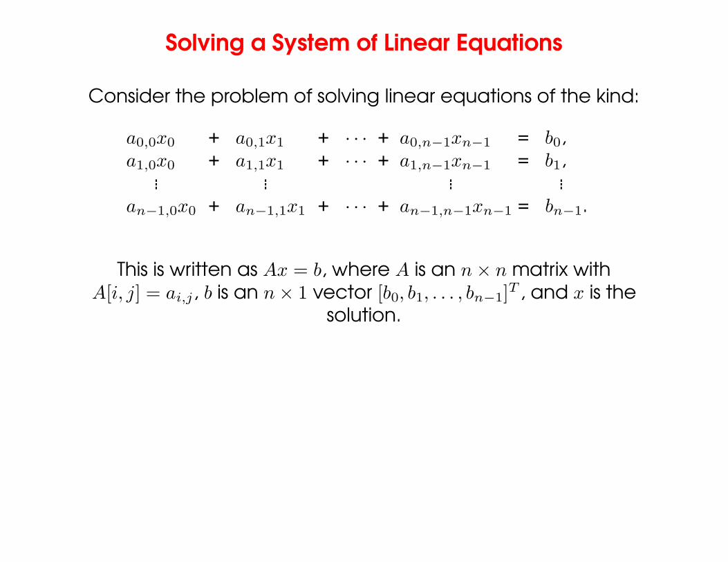
Consider the problem of solving linear equations of the kind:
a0,0x0 + a0,1x1 + · · · + a0,n−1xn−1 = b0,a1,0x0 + a1,1x1 + · · · + a1,n−1xn−1 = b1,
... ... ... ...an−1,0x0 + an−1,1x1 + · · · + an−1,n−1xn−1 = bn−1.
This is written as Ax = b, where A is an n × n matrix withA[i, j] = ai,j, b is an n × 1 vector [b0, b1, . . . , bn−1]
T , and x is thesolution.
– Typeset by FoilTEX – 28

Solving a System of Linear Equations
Two steps in solution are: reduction to triangular form, andback-substitution. The triangular form is as:
x0 + u0,1x1 + u0,2x2 + · · · + u0,n−1xn−1 = y0,x1 + u1,2x2 + · · · + u1,n−1xn−1 = y1,
... ...xn−1 = yn−1.
We write this as: Ux = y.
A commonly used method for transforming a given matrix intoan upper-triangular matrix is Gaussian Elimination.
– Typeset by FoilTEX – 29
Gaussian Elimimation
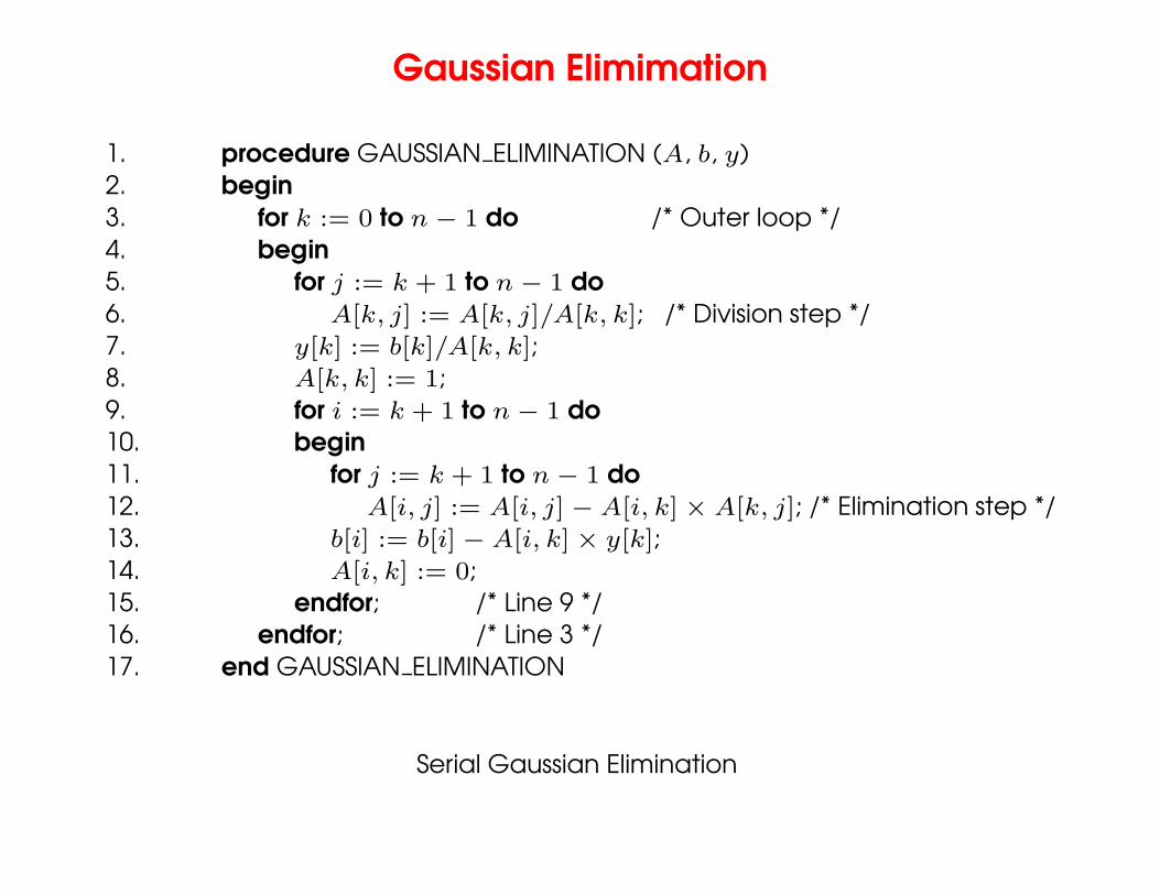
1. procedure GAUSSIAN ELIMINATION (A, b, y)2. begin3. for k := 0 to n − 1 do /* Outer loop */4. begin5. for j := k + 1 to n − 1 do6. A[k, j] := A[k, j]/A[k, k]; /* Division step */7. y[k] := b[k]/A[k, k];8. A[k, k] := 1;9. for i := k + 1 to n − 1 do10. begin11. for j := k + 1 to n − 1 do12. A[i, j] := A[i, j] − A[i, k] × A[k, j]; /* Elimination step */13. b[i] := b[i] − A[i, k] × y[k];14. A[i, k] := 0;15. endfor; /* Line 9 */16. endfor; /* Line 3 */17. end GAUSSIAN ELIMINATION
Serial Gaussian Elimination
– Typeset by FoilTEX – 30

Gaussian Elimination
• The computation has three nested loops – in the kth iteration ofthe outer loop, the algorithm performs (n − k)2 computations.Summing from k = 1..n, we have roughly (n3/3) multiplications-subtractions.
A[i,j] := A[i,j] - A[i,k] A[k,j]
Row k
Row i
(k,k) (k,j)
Inactive part
Active part
A[k,j] := A[k,j]/A[k,k]
x(i,k) (i,j)
Col
umn
k
Col
umn
j
A typical computation in Gaussian elimination.
– Typeset by FoilTEX – 31

Parallel Gaussian Elimination
• Assume p = n with each row assigned to a processor.
• The first step of the algorithm normalizes the row. This is a serialoperation and takes time (n − k) in the kth iteration.
• In the second step, the normalized row is broadcast to all theprocessors. This takes time (ts + tw(n − k − 1)) log n.
• Each processor can independently eliminate this row from itsown. This requires (n − k − 1) multiplications and subtractions.
• The total parallel time can be computed by summing from k =1..n − 1 as
TP =3
2n(n − 1) + tsn log n +
1
2twn(n − 1) log n. (8)
• The formulation is not cost optimal because of the tw term.
– Typeset by FoilTEX – 32

Parallel Gaussian EliminationP0
P
P
P
P
P
P
P1
2
3
4
5
6
7
P0
P
P
P
P
P
P
P1
2
3
4
5
6
7
P0
P
P
P
P
P
P
P1
2
3
4
5
6
7
(0,1) (0,2) (0,4)(0,3) (0,5) (0,6) (0,7) 1
0
0
0
0
0
1
1 (1,2) (1,3) (1,4) (1,5) (1,6) (1,7)
(2,3) (2,4) (2,5) (2,6) (2,7)
(4,3) (4,4) (4,5) (4,6) (4,7)
(5,3) (5,4) (5,5) (5,6) (5,7)
(6,4)(6,3) (6,6)(6,5) (6,7)
(7,3) (7,4) (7,5) (7,6) (7,7)
0
0
0
0
0
0
0
0
0
0
(b) Communication:
0 0
0
(3,3) (3,4) (3,5) (3,6) (3,7)
(0,1) (0,2) (0,4)(0,3) (0,5) (0,6) (0,7) 1
0
0
0
0
0
1
1 (1,2) (1,3) (1,4) (1,5) (1,6) (1,7)
(2,3) (2,4) (2,5) (2,6) (2,7)
(4,3) (4,4) (4,5) (4,6) (4,7)
(5,3) (5,4) (5,5) (5,6) (5,7)
(6,4)(6,3) (6,6)(6,5) (6,7)
(7,4) (7,5) (7,6) (7,7)
(3,5) (3,6) (3,7) 1
0
0
0
0
0
0
0
0
0
0
0
0 0
(0,1) (0,2) (0,4)(0,3) (0,5) (0,6) (0,7) 1
0
0
0
1
1 (1,2) (1,3) (1,4) (1,5) (1,6) (1,7)
(2,3) (2,4) (2,5) (2,6) (2,7)
(4,3) (4,4) (4,5) (4,6) (4,7)
(5,3) (5,4) (5,5) (5,6) (5,7)
(6,4)(6,3) (6,6)(6,5) (6,7)
(3,4) (3,5) (3,6) (3,7) 1
0
0
0
0
0
0
0
0
0
0 0
0
(3,4)
(7,3)
0 (7,3) (7,4) (7,5) (7,6) (7,7) 0 0
(c) Computation:
(a) Computation:
(i) A[k,j] := A[k,j]/A[k,k] for k < j < n
One-to-all brodcast of row A[k,*]
(ii) A[i,k] := 0 for k < i < n
for k < i < n and k < j < n
(ii) A[k,k] := 1
x(i) A[i,j] := A[i,j] - A[i,k] A[k,j]
Gaussian elimination steps during the iteration corresponding tok = 3 for an 8 × 8 matrix partitioned rowwise among eight
processes.
– Typeset by FoilTEX – 33

Parallel Gaussian Elimination: Pipelined Execution
• In the previous formulation, the (k+1)st iteration starts only afterall the computation and communication for the kth iteration iscomplete.
• In the pipelined version, there are three steps – normalizationof a row, communication, and elimination. These steps areperformed in an asynchronous fashion.
• A processor Pk waits to receive and eliminate all rows prior to k.Once it has done this, it forwards its own row to processor Pk+1.
– Typeset by FoilTEX – 34

Parallel Gaussian Elimination: Pipelined Execution
(4,1) (4,2) (4,4)
(3,1) (3,2) (3,3)
(1,1)
(3,4)
(1,2)
(2,3)
(1,4)
(2,1) (2,2) (2,3)
(c)
(f)(e) Iteration k = 1 starts
(k) (l)
(d)
(p) Iteration k = 4
(b)
(n) (o) Iteration k = 3 ends
(h)
(j) Iteration k = 1 ends
(m) Iteration k = 3 starts
(i) Iteration k = 2 starts
(a) Iteration k = 0 starts
(g) Iteration k = 0 ends
(0,4)
(1,4)
(4,4)
(3,4)
(0,2)(0,1) (0,3)
(1,3)
(4,3)
(3,3)(3,1) (3,2)
(4,1) (4,2)
(0,4)
(1,4)
(2,4)
(4,4)
(3,4)
(0,2)
(1,2)
(0,1) (0,3)
(1,3)
(2,3)
(4,3)
(3,3)
(1,1)
(2,2)(2,1)
(3,1) (3,2)
(4,1) (4,2)
(0,4)
(1,4)
(2,4)
(4,4)
(3,4)
(0,2)
(1,2)
(0,1) (0,3)
(1,3)
(2,3)
(4,3)
(3,3)
(2,2)(2,1)
(3,1) (3,2)
(4,0) (4,1) (4,2)
(0,4)
(2,4)
(4,4)
(3,4)
(0,2)(0,1) (0,3)
(2,3)
(4,3)
(3,3)
(2,2)(2,1)
(3,0) (3,1) (3,2)
(4,0) (4,1) (4,2)
1
0
1
0
0 0
0
1 1
0
0
0
(0,4)
(1,4)
(2,4)
(4,4)
(3,4)
(0,2)
(1,2)
(0,1) (0,3)
(1,3)
(2,3)
(4,3)
(3,3)
(1,1)
(2,2)
(1,0)
(2,0) (2,1)
(3,0) (3,1) (3,2)
(4,0) (4,1) (4,2)
(0,4)
(1,4)
(2,4)
(4,4)
(3,4)
(0,2)
(1,2)
(0,1) (0,3)
(1,3)
(2,3)
(4,3)
(3,3)
(1,1)
(2,2)
(1,0)
(2,0) (2,1)
(3,0) (3,1) (3,2)
(4,0) (4,1) (4,2)
(0,4)
(1,4)
(2,4)
(4,4)
(3,4)
(0,2)
(1,2)
(0,1) (0,3)
(1,3)
(2,3)
(4,3)
(3,3)
(1,1)
(2,2)(2,0) (2,1)
(3,0) (3,1) (3,2)
(4,0) (4,1) (4,2)
1(0,4)
(1,4)
(2,4)
(4,4)
(3,4)
(0,2)
(1,2)
(0,1) (0,3)
(1,3)
(2,3)
(4,3)
(3,3)
(0,0)
(1,1)
(2,2)
(1,0)
(2,0) (2,1)
(3,0) (3,1) (3,2)
(4,0) (4,1) (4,2)
1 1
(2,0)
(3,0)
(4,0)
1
(0,4)
(1,4)
(3,4)
(0,2)
(1,2)
(0,1) (0,3)
(1,3)
(2,3)
(0,4)
(1,4)
(2,4)
(4,4)
(3,4)
(0,2)
(1,2)
(0,1) (0,3)
(1,3)
(2,3)
(4,3)
(0,4)
(1,4)
(3,4)
(0,2)
(1,2)
(0,1) (0,3)
(1,3)
(4,3)
(0,4)
(1,4)
(2,4)
(3,4)
(0,2)
(1,2)
(0,1) (0,3)
(1,3)
(2,3)
(3,3)
1 1
0
1 1
0 0
0
0
0
0
0
1
0
0
0
0
1
0
1
0
0
0
0
1
0
0
(4,4)
(0,4)
(2,4)
(4,4)
(0,2)
(1,2)
(0,1) (0,3)
(1,3)
(4,3)(4,2)
(0,4)
(1,4)
(2,4)
(4,4)
(3,4)
(0,2)
(1,2)
(0,1) (0,3)
(1,3)
(2,3)
(4,3)
(3,3)(3,2)
(4,2)
(0,4)
(1,4)
(2,4)
(3,4)
(0,2)
(1,2)
(0,1) (0,3)
(2,3)
(3,3)
(0,4)
(1,4)
(4,4)
(0,2)
(1,2)
(0,1) (0,3)
(1,3)
(4,3)(4,1) (4,2)
1 1
0
1 1
0 0
0
0
0
0
0
1
0
0
0
0
1
0
1
0
0
0
0
1
0
0
0
0 0
0
1 1 1
0 0
0 0
Communication for k = 2 Computation for k = 2
0
Communication for k = 1
Communication for k = 0, 3 Computation for k = 0, 3
Computation for k = 1, 4
(3,2)
(1,0)
1
0
0
0
0
0
0
0
(1,3)
1
(3,2)
0
1 1
1
0
0
(1,4)
(2,3)
(1,2)
0
(2,3) (2,4)
1 0
0
1
(2,4)
0
0 0
1
(2,2) (2,4)
(4,3)
(4,2) (4,3) (4,4) (4,4)
(3,3) (3,4)
(2,4)
(1,3)
Pipelined Gaussian elimination on a 5 × 5 matrix partitioned withone row per process.
– Typeset by FoilTEX – 35

Parallel Gaussian Elimination: Pipelined Execution
• The total number of steps in the entire pipelined procedure isΘ(n).
• In any step, either O(n) elements are communicated betweendirectly-connected processes, or a division step is performedon O(n) elements of a row, or an elimination step is performedon O(n) elements of a row.
• The parallel time is therefore O(n2).
• This is cost optimal.
– Typeset by FoilTEX – 36

Parallel Gaussian Elimination: Pipelined ExecutionP0
(0,1) (0,2) (0,4)(0,3) (0,5) (0,6) (0,7) 1
0
0
0
0
0
1
1 (1,2) (1,3) (1,4) (1,5) (1,6) (1,7)
(2,3) (2,4) (2,5) (2,6) (2,7)
(4,3) (4,4) (4,5) (4,6) (4,7)
(5,3) (5,4) (5,5) (5,6) (5,7)
(6,4)(6,3) (6,6)(6,5) (6,7)
(7,3) (7,4) (7,5) (7,6) (7,7)
(3,4) (3,6) (3,7) 1
0
0
0
0
0
0
0
0
0
0
0
0 0
(3,5)
P
P
P1
2
3
The communication in the Gaussian elimination iterationcorresponding to k = 3 for an 8 × 8 matrix distributed among four
processes using block 1-D partitioning.
– Typeset by FoilTEX – 37

Parallel Gaussian Elimination: Block 1D with p < n
• The above algorithm can be easily adapted to the case whenp < n.
• In the kth iteration, a processor with all rows belonging to theactive part of the matrix performs (n − k − 1)n/p multiplicationsand subtractions.
• In the pipelined version, for n > p, computation dominatescommunication.
• The parallel time is given by: 2(n/p)Σn−1k=0(n − k − 1), or
approximately, n3/p.
• While the algorithm is cost optimal, the cost of the parallelalgorithm is higher than the sequential run time by a factor of3/2.
– Typeset by FoilTEX – 38

Parallel Gaussian Elimination: Block 1D with p < n
(b) Cyclic 1-D mapping(a) Block 1-D mapping
(7,3)
(3,3)
0
0
0
0
0
0
(0,7)
(7,7)
(3,7)
(6,7)
(2,7)
(5,7)
(1,7)
(4,7)
(0,1)
0
0
0
0
0
1
0
(0,2)
0
0
0
1
0
(1,2)
0
(0,3)
(7,3)
(6,3)
(2,3)
(5,3)
(1,3)
(4,3)
(3,3)
(0,4)
(7,4)
(3,4)
(6,4)
(2,4)
(5,4)
(1,4)
(4,4)
(0,6)
(7,6)
(3,6)
(6,6)
(2,6)
(5,6)
(1,6)
(4,6)
(0,5)
(7,5)
(3,5)
(6,5)
(2,5)
(5,5)
(1,5)
(4,5)P0 P0
P
P
P
(0,1)
1
(0,3)
2
3 P
P
P1
2
3
1 (1,3)
(2,3)
(4,3)
(5,3)
(0,4) (0,5) (0,6) (0,7) 1
0
(1,4) (1,5) (1,6) (1,7)
(2,4) (2,5) (2,6) (2,7)
(4,4) (4,5) (4,6) (4,7)
(5,4) (5,5) (5,6) (5,7)
(6,4) (6,6)(6,5) (6,7)
(7,4) (7,5) (7,6) (7,7)
(3,4) (3,5) (3,6) (3,7)
0
0
0
0
0
0
1(0,2)
0
0
0
0
1
(1,2)
0
0
0
0
0
0
0
0
(6,3)
Computation load on different processes in block and cyclic 1-Dpartitioning of an 8 × 8 matrix on four processes during the
Gaussian elimination iteration corresponding to k = 3.
– Typeset by FoilTEX – 39

Parallel Gaussian Elimination: Cyclic 1D Mapping
• The load imbalance problem can be alleviated by using acyclic mapping.
• In this case, other than processing of the last p rows, there is noload imbalance.
• This corresponds to a cumulative load imbalance overhead ofO(n2p) (instead of O(n3) in the previous case).
– Typeset by FoilTEX – 40

Parallel Gaussian Elimination: 2-D Mapping
• Assume an n × n matrix A mapped onto an n × n mesh ofprocessors.
• Each update of the partial matrix can be thought of as ascaled rank-one update (scaling by the pivot element).
• In the first step, the pivot is broadcast to the row of processors.
• In the second step, each processor locally updates its value.For this it needs the corresponding value from the pivot row,and the scaling value from its own row.
• This requires two broadcasts, each of which takes log n time.
• This results in a non-cost-optimal algorithm.
– Typeset by FoilTEX – 41

Parallel Gaussian Elimination: 2-D Mapping
(d) A[i,j] := A[i,j]-A[i,k] A[k,j]
(a) Rowwise broadcast of A[i,k] (b) A[k,j] := A[k,j]/A[k,k]
(c) Columnwise broadcast of A[k,j]
(0,1) (0,2) (0,4)(0,3) (0,5) (0,6) (0,7) 1
0
0
0
0
0
1
1 (1,2) (1,3) (1,4) (1,5) (1,6) (1,7)
(2,3) (2,4) (2,5) (2,6) (2,7)
(4,3) (4,4) (4,5) (4,6) (4,7)
(5,3) (5,4) (5,5) (5,6) (5,7)
(6,4)(6,3) (6,6)(6,5) (6,7)
(7,3) (7,4) (7,5) (7,6) (7,7)
(3,3) (3,4) (3,5) (3,6) (3,7)
(0,1) (0,2) (0,4)(0,3) (0,5) (0,6) (0,7) 1
0
0
0
0
0
1
1 (1,2) (1,3) (1,4) (1,5) (1,6) (1,7)
(2,3) (2,4) (2,5) (2,6) (2,7)
(4,3) (4,5) (4,6) (4,7)
(5,4)
(4,4)
(5,5) (5,6) (5,7)
(6,4)(6,3) (6,6)(6,5) (6,7)
(7,4) (7,5) (7,6) (7,7)
(3,4) (3,5) (3,6) (3,7) 1
(0,1) (0,2) (0,4)(0,3) (0,5) (0,6) (0,7) 1
0
0
0
0
0
1
1 (1,2) (1,3) (1,4) (1,5) (1,6) (1,7)
(2,3) (2,4) (2,5) (2,6) (2,7)
(4,3) (4,4) (4,5) (4,6) (4,7)
(5,3) (5,4) (5,5) (5,6) (5,7)
(6,4)(6,3) (6,6)(6,5) (6,7)
(7,3) (7,4) (7,5) (7,6) (7,7)
(3,4) (3,5) (3,6) (3,7) 1
0
0
0
0
0
0
0
0
0
0
0
0
0
0
0
(0,1) (0,2) (0,4)(0,3) (0,5) (0,6) (0,7) 1
0
0
0
0
0
1
1 (1,2) (1,3) (1,4) (1,5) (1,6) (1,7)
(2,3) (2,4) (2,5) (2,6) (2,7)
(4,3) (4,4) (4,5) (4,6) (4,7)
(5,3) (5,4) (5,5) (5,6) (5,7)
(6,4)(6,3) (6,6)(6,5) (6,7)
(7,3) (7,4) (7,5) (7,6) (7,7)
0
0
0
0
0
0
0
0
0
0
0
0
0
0
0
0
0
0
0
0
0
0
0
0
0
0
0 0 0 0
0
0 0
0
0 0
0
(3,3) (3,4) (3,5) (3,6) (3,7)
for (k - 1) < i < n for k < j < n
for k < j < n
(5,3)
for k < i < n and k < j < nx
(7,3)
Various steps in the Gaussian elimination iteration correspondingto k = 3 for an 8 × 8 matrix on 64 processes arranged in a logical
two-dimensional mesh.
– Typeset by FoilTEX – 42

Parallel Gaussian Elimination: 2-D Mapping withPipelining
• We pipeline along two dimensions. First, the pivot value ispipelined along the row. Then the scaled pivot row is pipelineddown.
• Processor Pi,j (not on the pivot row) performs the eliminationstep A[i, j] := A[i, j]−A[i, k]×A[k, j] as soon as A[i, k] and A[k, j]are available.
• The computation and communication for each iteration movesthrough the mesh from top-left to bottom-right as a “front.”
• After the front corresponding to a certain iteration passesthrough a process, the process is free to perform subsequentiterations.
• Multiple fronts that correspond to different iterations are activesimultaneously.
– Typeset by FoilTEX – 43

Parallel Gaussian Elimination: 2-D Mapping withPipelining
• If each step (division, elimination, or communication) isassumed to take constant time, the front moves a single step inthis time. The front takes Θ(n) time to reach Pn−1,n−1.
• Once the front has progressed past a diagonal processor, thenext front can be initiated. In this way, the last front passes thebottom-right corner of the matrix Θ(n) steps after the first one.
• The parallel time is therefore O(n), which is cost-optimal.
– Typeset by FoilTEX – 44

2-D Mapping with Pipelining
(p) Iteration k = 0 ends(n)
(i)
(a) Iteration k = 0 starts
(g) Iteration k = 1 starts(e)
(d)(c)(b)
(h)
(m) Iteration k = 2 starts
(l)(k) (j)
(o)
(f)
Communication for k = 1
Communication for k = 0
(1,4)
(2,4)
(4,4)
(3,4)
(0,2)(0,1) (0,3)
(1,3)
(2,3)
(4,3)
(3,3)
(2,2)(2,1)
(3,1) (3,2)
(4,1) (4,2)
(0,4)
(1,4)
(2,4)
(4,4)
(3,4)
(0,2)
(1,2)
(0,1) (0,3)
(1,3)
(2,3)
(4,3)
(3,3)
(1,1)
(2,2)(2,1)
(3,1) (3,2)
(4,1) (4,2)
(0,4)
(1,4)
(2,4)
(4,4)
(3,4)
(0,2)
(1,2) (1,3)
(4,3)
(3,3)
(1,1)
(2,2)(2,1)
(3,1) (3,2)
(4,0) (4,1) (4,2)
(0,4)
(1,4)
(2,4)
(4,4)
(1,2)
(0,1) (0,3)
(1,3)
(2,3)
(4,3)
(3,3)
(1,1)
(2,2)(2,1)
(3,0) (3,1) (3,2)
(4,0) (4,1) (4,2)
1
0
1
0
0 0
0
1 1
0
0
0
(0,4)
(0,4)
(1,4)
(2,4)
(4,4)
(3,4)
(0,2)
(1,2)
(0,1) (0,3)
(1,3)
(2,3)
(4,3)
(3,3)
(1,1)
(2,2)
(1,0)
(2,0) (2,1)
(3,0) (3,1) (3,2)
(4,0) (4,1) (4,2)
(0,4)
(1,4)
(2,4)
(4,4)
(3,4)
(0,2)
(1,2)
(0,1) (0,3)
(1,3)
(2,3)
(4,3)
(3,3)
(1,1)
(2,2)
(1,0)
(2,0) (2,1)
(3,0) (3,1) (3,2)
(4,0) (4,1) (4,2)
(0,4)
(1,4)
(2,4)
(4,4)
(3,4)
(0,2)
(1,2)
(0,1) (0,3)
(1,3)
(2,3)
(4,3)
(3,3)
(1,1)
(2,2)(2,0) (2,1)
(3,0) (3,1) (3,2)
(4,0) (4,1) (4,2)
1(0,4)
(1,4)
(2,4)
(4,4)
(3,4)
(0,2)
(1,2)
(0,1) (0,3)
(1,3)
(2,3)
(4,3)
(3,3)
(0,0)
(1,1)
(2,2)
(1,0)
(2,0) (2,1)
(3,0) (3,1) (3,2)
(4,0) (4,1) (4,2)
1 1
0
(2,0)
(3,0) (3,0)
(4,0) (4,0)
1
(0,4)
(1,4)
(4,4)
(3,4)
(0,2)
(1,2)
(0,1) (0,3)
(1,3)
(2,3)
(4,2)
(0,4)
(1,4)
(2,4)
(4,4)
(3,4)
(0,2)
(1,2)
(0,1) (0,3)
(1,3)
(2,3)
(4,3)
(3,3)(3,2)
(4,2)
(0,4)
(1,4)
(3,4)
(0,2)
(1,2)
(0,1) (0,3)
(1,3)
(4,3)
(3,2)
(0,4)
(1,4)
(2,4)
(4,4)
(3,4)
(0,2)
(1,2)
(0,1) (0,3)
(1,3)
(2,3)
(4,3)
(3,3)
(2,2)
(3,2)
(4,1) (4,2)
1 1
0
1 1
0 0
0
0
0
0
0
1
0
0
0
0
1
0
1
0
0
0
0
1
0
0
(4,4)
(0,1)
(0,4)
(2,4)
(4,4)
(3,4)
(0,2)
(1,2)
(0,1) (0,3)
(1,3)
(4,3)
(3,3)
(2,2)
(4,2)
(0,4)
(1,4)
(2,4)
(4,4)
(3,4)
(0,2)
(1,2)
(0,1) (0,3)
(1,3)
(2,3)
(4,3)
(3,3)
(2,2)
(3,2)
(4,1) (4,2)
(0,4)
(1,4)
(2,4)
(3,4)
(0,2)
(1,2)
(0,1) (0,3)
(2,3)
(4,3)
(3,3)(3,1) (3,2)
(4,1) (4,2)
(0,4)
(1,4)
(2,4)
(4,4)
(3,4)
(0,2)
(1,2)
(0,1) (0,3)
(1,3)
(2,3)
(4,3)
(3,3)
(2,2)(2,1)
(3,1) (3,2)
(4,1) (4,2)
1 1
0
1 1
0 0
0
0
0
0
0
1
0
0
0
0
1
0
1
0
0
0
0
1
0
0
(0,3)
(2,3)
(4,0) (4,4)
(3,1)
(4,1)
(3,4)
0
0 0
0
1 1 1
0 0
0 0
Communication for k = 2
Computation for k = 0
Computation for k = 1
Computation for k = 2
0
(2,2)
(1,3)
(3,2)
(2,3)
(1,4)
(1,2)
(4,2)
(3,3)
(2,3) (2,4)
(4,3)
(3,3)
(2,4)
(0,2)
Pipelined Gaussian elimination for a 5 × 5 matrix with 25 processors.
– Typeset by FoilTEX – 45

Parallel Gaussian Elimination: 2-D Mapping withPipelining and p < n
• In this case, a processor containing a completely active part ofthe matrix performs n2/p multiplications and subtractions, andcommunicates n/
√p words along its row and its column.
• The computation dominantes communication for n >> p.
• The total parallel run time of this algorithm is (2n2/p) × n, sincethere are n iterations. This is equal to 2n3/p.
• This is three times the serial operation count!
– Typeset by FoilTEX – 46

Parallel Gaussian Elimination: 2-D Mapping withPipelining and p < n
(a) Rowwise broadcast of A[i,k] (b) Columnwise broadcast of A[k,j]for i = k to (n - 1)
(0,4) (0,5) (0,6) (0,7) 1
0
(1,5)(1,4) (1,7)
(2,4) (2,5) (2,6) (2,7)
(4,4) (4,5) (4,6) (4,7)
(5,4) (5,5) (5,6) (5,7)
(6,4) (6,6)(6,5) (6,7)
(7,4) (7,5) (7,6) (7,7)
(3,4) (3,5) (3,6) (3,7)
0
0
0
0
0
0
(0,1) (0,2) (0,4)(0,3) (0,5) (0,6) (0,7)
0
(1,6)
0
1
0
0
1
1 (1,2) (1,3) (1,4) (1,5) (1,6) (1,7)
(2,3) (2,4) (2,5) (2,6) (2,7)
(4,3) (4,4) (4,5) (4,6) (4,7)
(5,3) (5,4) (5,5) (5,6) (5,7)
(6,4)(6,3) (6,6)(6,5) (6,7)
(7,3) (7,4) (7,5) (7,6) (7,7)
(3,4) (3,5) (3,6) (3,7) 1
0
0
0
0
0
0
0
0
0
0
0
0 0
(0,2)
0
0
0
0
1
(1,2)
0
for j = (k + 1) to (n - 1)
(0,1)
1
(2,3)
(4,3)
(5,3)
(6,3)
(7,3)
(3,3)
0
0
0
0
0
0
(0,3)
(1,3)
0PSfrag replacementsn√p
n/√
pn
n
The communication steps in the Gaussian elimination iterationcorresponding to k = 3 for an 8 × 8 matrix on 16 processes of a
two-dimensional mesh.
– Typeset by FoilTEX – 47

Parallel Gaussian Elimination: 2-D Mapping withPipelining and p < n
(a) Block-checkerboard mapping (b) Cyclic-checkerboard mapping
0
0
0
0
(0,7)
0
(3,7)
(7,7)
(2,7)
(5,7)
(1,7)
(4,7)
(0,1)
0
(6,7) 0
0
0
1
0
(0,2)
0
0
0
1
0
(1,2)
0
(0,3)
0
0 (2,3)
(5,3)
(1,3)
(4,3)
(3,3)
(7,3)(7,4)
(3,4)
(6,4)
(2,4)
(5,4)
(1,4)
(4,4)
(0,5)
(7,5)
(3,5)
(6,5)
(2,5)
(5,5)
(1,5)
(4,5)
(0,6)
(7,6)
(3,6)
(6,6)
(2,6)
(5,6)
(1,6)
(4,6)
(6,3)
(7,3)
(3,3)(6,3)
(5,3)
(4,3)
(2,3)
(1,3) 1
(0,4)(0,3) (0,4) (0,5) (0,6) (0,7) 1
0
(1,4) (1,5) (1,6) (1,7)
(2,4) (2,5) (2,6) (2,7)
(4,4) (4,5) (4,6) (4,7)
(5,4) (5,5) (5,6) (5,7)
(6,4) (6,6)(6,5) (6,7)
(7,4) (7,5) (7,6) (7,7)
(3,4) (3,5) (3,6) (3,7)
0
0
0
0
0
0
1(0,2)
0
0
0
0
1
(1,2)
0
0
0
0
0
0
0
0
(0,1)
Computational load on different processes in block and cyclic2-D mappings of an 8 × 8 matrix onto 16 processes during the
Gaussian elimination iteration corresponding to k = 3.
– Typeset by FoilTEX – 48

Parallel Gaussian Elimination: 2-D Cyclic Mapping
• The idling in the block mapping can be alleviated using acyclic mapping.
• The maximum difference in computational load between anytwo processes in any iteration is that of one row and onecolumn update.
• This contributes Θ(n√
p) to the overhead function. Since thereare n iterations, the total overhead is Θ(n2√p).
– Typeset by FoilTEX – 49

Gaussian Elimination with Partial Pivoting
• For numerical stability, one generally uses partial pivoting.
• In the kth iteration, we select a column i (called the pivotcolumn) such that A[k, i] is the largest in magnitude among allA[k, j] such that k ≤ j < n.
• The kth and the ith columns are interchanged.
• Simple to implement with row-partitioning and does not addoverhead since the division step takes the same time ascomputing the max.
• Column-partitioning, however, requires a global reduction,adding a log p term to the overhead.
• Pivoting precludes the use of pipelining.
– Typeset by FoilTEX – 50

Gaussian Elimination with Partial Pivoting: 2-DPartitioning
• Partial pivoting restricts use of pipelining, resulting in performanceloss.
• This loss can be alleviated by restricting pivoting to specificcolumns.
• Alternately, we can use faster algorithms for broadcast.
– Typeset by FoilTEX – 51

Solving a Triangular System: Back-Substitution
• The upper triangular matrix U undergoes back-substitution todetermine the vector x.
1. procedure BACK SUBSTITUTION (U , x, y)2. begin3. for k := n − 1 downto 0 do /* Main loop */4. begin5. x[k] := y[k];6. for i := k − 1 downto 0 do7. y[i] := y[i] − x[k] × U [i, k];8. endfor;9. end BACK SUBSTITUTION
A serial algorithm for back-substitution.
– Typeset by FoilTEX – 52

Solving a Triangular System: Back-Substitution
• The algorithm performs approximately n2/2 multiplications andsubtractions.
• Since complexity of this part is asymptotically lower, we shouldoptimize the data distribution for the factorization part.
• Consider a rowwise block 1-D mapping of the n × n matrix Uwith vector y distributed uniformly.
• The value of the variable solved at a step can be pipelinedback.
• Each step of a pipelined implementation requires a constantamount of time for communication and Θ(n/p) time forcomputation.
• The parallel run time of the entire algorithm is Θ(n2/p).
– Typeset by FoilTEX – 53

Solving a Triangular System: Back-Substitution
• If the matrix is partitioned by using 2-D partitioning on a√
p ×√p logical mesh of processes, and the elements of the vector
are distributed along one of the columns of the process mesh,then only the
√p processes containing the vector perform any
computation.
• Using pipelining to communicate the appropriate elements ofU to the process containing the corresponding elements of yfor the substitution step (line 7), the algorithm can be executedin Θ(n2/
√p) time.
• While this is not cost optimal, since this does not dominante theoverall computation, the cost optimality is determined by thefactorization.
– Typeset by FoilTEX – 54
Related Documents