Using clustering for document reconstruction

Using Clustering for Document Reconstruction

Anna Ukovicha, Alessandra Zacchignab, Giovanni Ramponia, Gabriella Schoierba DEEI, University of Trieste, Trieste, Italyb DiSES, University of Trieste, Trieste, Italy

ABSTRACTIn the forensics and investigative science fields there may arise the need of reconstructing documents whichhave been destroyed by means of a shredder. In a computer-based reconstruction, the pieces are described bynumerical features, which represent the visual content of the strips. Usually, the pieces of different pages havebeen mixed. We propose an approach for the reconstruction which performs a first clustering on the strips toease the successive matching, be it manual (with the help of a computer) or automatic. A number of features,extracted by means of image processing algorithms, have been selected for this aim. The results show theeffectiveness of the features and of the proposed clustering algorithm.

Keywords: document reconstruction; hierarchical clustering; jigsaw puzzle.

1. PROBLEM DEFINITIONThe reconstruction of shredded or torn documents is a problem which may arise in the forensics and investigativescience fields. Image processing techniques give the opportunity for a computer-based reassembly.

The typical documents which one may need to reconstruct are office documents, such as printed text doc-uments, or handwritten notebook paper. In general, the different pages which have been shredded may havedifferent font format, ink color, page layout.

For a computer-aided reconstruction the strips need to be first acquired by means of a scanner, then segmentedfrom the background. At this point features describing their visual content are extracted.1 The visual contentneeds to be extracted, because the piece contour shape, which is commonly used in the automatic jigsaw puzzleassembly, is not very useful here, since the strips have approximately all the same shape (long and narrowrectangular strips). Once the strips are described by the features, the search for matching pieces is the searchfor pieces which are similar in the feature space.

In this work we will focus on strip-cut shredded documents for which the cutting direction is orthogonal tothe text direction.

In the following, the visual features, which are automatically extracted from the strips, are described. More-over, the case of blank strips is discussed.

1.1. Feature descriptionA set of features for describing the visual content of the strips has been defined.1 We recall here some of themwhich are suitable in particular for printed text: the line spacing, the page layout appearance (position of thefirst and last line of text, number of lines of text), paper/ink color, text edge energy.

The line spacing feature LS is useful for distinguishing among remnants coming from different documents.The vertical projection profile of the strip is evaluated, and its Discrete Fourier Transform (DFT) is computed.The first harmonic detected in the transformed domain corresponds to the fundamental frequency. This is theline spacing LS.

Once the line spacing LS has been extracted, the text line positions are calculated from the cross-correlationof the vertical projection profile and the sinusoidal wave at frequency LS translated along the vertical projectionsignal height. The resulting line positions (in pixel) are represented by the array:

L = l1, l2 . . . , lNLINE . (1)

The other features can be extracted from the feature L. These are the following (where height representsthe strip image height in pixel):

• number of lines of text NLINENLINE = ] L, (2)

where ] represents the cardinality of a set;

• relative position of the first line of text FIRSTL

FIRSTL =l1

height; (3)

• relative position of the last line of text LASTL

LASTL =∑NLINE

i=1 liheight

. (4)

NLINE, FIRSTL, LASTL are scalar numbers. LASTL and FIRSTL have values between 0 and 1.

In the case of either printed or handwritten text, the text appearance can be extracted by edge descriptors.The handwriting style in particular can have preferred directions of strikes. In the case of printed text, differentfont style may have been used, such as italics or bold. The feature for extracting edges relies on the Robinsonoperator in four directions, horizontal, vertical, two diagonals, applied to the gray value remnant image. Theenergy of edges in the four directions is evaluated as the average of the squared edge values in the strips.

Both the paper type and the color of the ink are useful information for finding the matching pieces. Back-ground and ink regions are separated by means of an Otsu thresholding. The features are extracted in theYCbCr color space. The paper (ink) dominant color is represent by the most frequent Y, Cb, Cr values in thepaper (ink) region.

1.2. Blank strips

In particular in the case of printed text, the page margins contain no text and the corresponding strips are thusblank. During the reconstruction, this kind of strips can be eliminated from the dataset, because they containno relevant information to be recovered by means of the reconstruction and they can not be distinguished onefrom the other, unless different paper types are used. With the term blank we mean also squared paper or linedpaper strips with no text (either handwritten or printed).

In Ref.2 the number of blank strips for printed text documents are estimated to be approximately 20% of thetotal number of strips.

In order to identify them, appropriate features must be used. For example, if the feature NLINE is equalto 0, then the strip is catalogued as blank and it is not considered for the successive analysis.

2. APPROACH TO THE SOLUTION

Our approach for the reconstruction of shredded documents is based on a clustering strategy. Our aim is togroup together the pieces originally belonging to the same page. The following search for matching remnantsis conducted within smaller subsets instead of within the whole set of remnants. Ideally, we would like to findP subsets if P pages have been destroyed. The approach is similar to the methodology a human being usesfor reassembling a jigsaw puzzle. The pieces with a similar content, usually the color, are grouped together,and matches are first searched within these groups. Although the methodology is described here for strip-cutshredded document reconstruction, it could be also applied to jigsaw puzzle assembly and reconstruction fromfragments.3

The first clustering step is useful in the case of computer-aided reconstruction as well as in the case of fully-automatic reconstruction. In both cases, the computational complexity of the search for matching pieces canbe reduced, if the search is limited to one cluster instead of to the whole dataset. Indeed, if we suppose to usebinary features (this is reasonable because each feature can be coded as a sequence of binary features), then theminimum number of features for distinguishing among pages (to univocally identify a page) is log2 P , where P

is the number of pages. This is smaller than the minimum number of features needed for the exact matching,which consists of an ordering of the strips in the different pages (the latter is related to the total number ofelements in the dataset, N). With a clustering, the similarity between pieces can be firstly evaluated on somegeneral page-related features, and then, the search can be restricted to pieces belonging to the same cluster,using the more precise features.

When a semi-automatic reconstruction is performed, a human operator makes a virtual reconstruction on thecomputer. A virtual strip a is picked up and the two matching pieces are searched. The Q most similar pieces,according to some similarity measure on the feature values, are presented to the user. If a clustering is firstperformed, then the Q most similar pieces are searched inside the cluster instead of inside the whole dataset.Then if the two matching pieces are found, the strip is removed from the dataset, and the search starts againwith another piece.

It can be argued that in the case of semi-automatic reconstruction the process of clustering similar piecescan be done by a human being as well. This can be true if the classes, i.e. the pages, from which the remnantscome from are very different one from the other, but otherwise it can be difficult and boring to try to identifydifferences for example in line spacing or in the number of lines. See, for example, Figure 1: it is difficult toinstantaneously recognize the difference in line spacing between the first two strips . However, the extracted LSvalues are able to distinguish between the pieces.

In order to perform the clustering, two steps must be first accomplished: the most discriminant features haveto be selected, and the number of clusters to be created must be defined.

3. FEATURE SELECTION

The selection of the features which could yield a good clustering depends on the specific dataset considered. Forexample, the background color feature will work well only if the original pages have different types of paper. Ifwe do not have enough a priori knowledge about the dataset characteristics, then an automatic criterion mustbe defined to choose the most relevant ones.

The criterion we adopt is the correlation measure. If two features show to have a high correlation in thespecific dataset examined, then just one of these features is considered for the clustering. Indeed, the otherfeature does not bring more information for characterizing the strips, and it could instead reduce the algorithmperformance. The correlation coefficient between the two features fj and fk is defined as:

rfj ,fk=

N∑

fjfk − (∑

fj)(∑

fk)√N(

∑f2

j )− (∑

fj)2√

N(∑

f2k )− (

∑fk)2

, (5)

where N is the number of strips in the dataset.

4. HOW MANY CLUSTERS?

The problem of finding the best number of cluster is sometimes referred to as the cluster validity problem.

In an ideal case, the choice of the number of clusters is trivial. Indeed, if the dataset contains N strips, andwe suppose there are no missing pieces and we know the exact number of pieces n in which a page is cut (i.e.the shredded device used is known), then the number of clusters we have to look for is equal to N/n if we wantto group together the strips originally belonging to the same page.

In the non-ideal case, however, the following situation can change the number of clusters:

1. Some of the features are likely to change their value going from strips in the left portion of a page to thosein the right portion; for example, the number of lines of text NLINE is usually decreasing. According tothese features, for some pages it is unlikely that the page left-side strips and the page right-side strips areput in the same cluster.

2. There are outlier strips, in particular close to the page margins: they are likely to be classified as singletonclusters

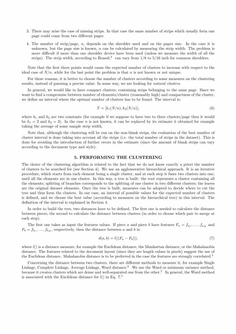
3. There may arise the case of missing strips. In that case the same number of strips which usually form onepage could come from two different pages

4. The number of strip/page, n, depends on the shredder used and on the paper size. In the case it isunknown, but the page size is known, n can be calculated by measuring the strip width. The problem ismore difficult if more than one shredder device have been used (unless we measure the width of all thestrips). The strip width, according to Brassil,4 can vary from 1/8 to 5/16 inch for common shredders.

Note that the first three points would cause the expected number of clusters to increase with respect to theideal case of N/n, while for the last point the problem is that n is not known or not unique.

For these reasons, it is better to choose the number of clusters according to some measures on the clusteringresults, instead of guessing a precise value. In some way, we are looking for natural clusters.

In general, we would like to have compact clusters, containing strips belonging to the same page. Since wewant to find a compromise between number of elements/cluster (reasonably high) and compactness of the cluster,we define an interval where the optimal number of clusters has to be found. The interval is:

T = [k1(N/n), k2(N/n)], (6)

where k1 and k2 are two constants (for example if we suppose to have two to three clusters/page then it wouldbe k1 = 2 and k2 = 3). In the case n is not known, it can be replaced by its estimate n obtained for exampletaking the average of some sample strip width.

Note that, although the clustering will be run on the non-blank strips, the evaluation of the best number ofcluster interval is done taking into account all the strips (i.e. the total number of strips in the dataset). This isdone for avoiding the introduction of further errors in the estimate (since the amount of blank strips can varyaccording to the document type and style).

5. PERFORMING THE CLUSTERING

The choice of the clustering algorithm is related to the fact that we do not know exactly a priori the numberof clusters to be searched for (see Section 4). We use an agglomerative hierarchical approach. It is an iterativeprocedure, which starts from each element being a single cluster, and at each step it fuses two clusters into one,until all the elements are in one cluster. In this way, a tree is built: the root represents a cluster containing allthe elements; splitting of branches corresponds to the splitting of one cluster in two different clusters; the leavesare the original dataset elements. Once the tree is built, measures can be adopted to decide where to cut thetree and thus form the clusters. In our case, an interval of possible values for the expected number of clustersis defined, and we choose the best value (according to measures on the hierarchical tree) in this interval. Thedefinition of the interval is explained in Section 4.

In order to build the tree, two distances have to be defined. The first one is needed to calculate the distancebetween pieces, the second to calculate the distance between clusters (in order to choose which pair to merge ateach step).

The first one takes as input the features values. If piece a and piece b have features Fa = fa1 , . . . , faM andFb = fb1 , . . . , fbM

, respectively, then the distance between a and b is:

d(a, b) = l(||Fa − Fb||), (7)

where l() is a distance measure, for example the Euclidean distance, the Manhattan distance, or the Mahalanobisdistance. The features related to the document layout (since they are length values in pixels) suggest the use ofthe Euclidean distance. Mahalanobis distance is to be preferred in the case the features are strongly correlated.5

Concerning the distance between two clusters, there are different methods to measure it, for example SingleLinkage, Complete Linkage, Average Linkage, Ward distance.6 We use the Ward or minimum variance method,because it creates clusters which are dense and well-separated one from the other.5 In general, the Ward methodis associated with the Euclidean distance for l() in Eq. 7.5

The Ward method aims to merge at each step the two clusters which minimize the overall squared error ofthe clustering. The squared error for cluster k is7:

e2k =

nk∑

i=1

M∑

j=1

[f (k)ij −m

(k)j ]2, (8)

where f(k)ij is the value for feature j of strip i, nk is the number of strips in cluster k, M is the dimensionality of

the feature space, m(k)j is the centroid of cluster k, calculated as:

m(k)j =

1nk

nk∑

i=1

f(k)ij (9)

The squared error for the entire clustering is :

E2K =

K∑

k=1

e2k, (10)

where K is the number of clusters at the current step.

E2K is minimum (equal to 0) if each strip is one cluster. According to the Ward method, the pair of clusters

p and q that minimizes ∆E2pq, i.e. the change in EK caused by the merger of clusters p and q into cluster t, is

chosen.

5.1. Pruning the treeOnce the tree is built, the selection of number of clusters is conducted in the interval defined in Section 4.

In the previous section, the processing of merging clusters can be visualized as a tree. The leaves are thedataset elements, while the root represents the cluster which contains all the elements. Branches go from theleaves to the root, successively merging from two into one. Each node (connection of three branches) has a heighthn corresponding to the effort the algorithm made in merging two clusters (two nodes in the tree) into one atthe step n. The leaves have height 0 and the height is increasing going towards the root.

In our case, hn = E2K of Eq. 10, with K = N − n (indeed, at step 1 two elements are merged and we have

K = N − 1 clusters, at step n K = 1 cluster is formed).

The heights hn are non decreasing, with n = 1, . . . , N − 1.

The ratio between two successive values of the heights is defined as:

sn =hn+1

hn, (11)

with n = 1, . . . , N−2. If sn is high for a given n, this means the two clusters which have been merged at the step(n+1) were likely to remain two separate clusters, thus the number of clusters should better stay at K = N −n.

Since we are looking for natural clusters in the interval T defined in Equation 6, we have to look for localmaxima of sn in the interval with K = N − n belonging to T . The optimal number of clusters is thus topt with:

s(N−topt) = maxt∈T

s(N−t). (12)

5.2. Refinement with K-meansOnce the optimal number of clusters has been found, the clusters are formed cutting the hierarchical treeaccording to the selected number of clusters. At this point the clusters centers are taken as the initial centersfor a K-means clustering operation.6 This is a partitive clustering algorithm. The K-means clustering has theaim of refining the result obtained by the hierarchical approach.

K-means is an iterative procedure which consists, at each step, in assigning the elements to the cluster withthe closest cluster center (the Euclidean distance is used for the measure), and then computing again the centers.The procedure stops when the maximum number of iterations is reached or when there are no changes in thecenters values.

6. EXPERIMENTAL RESULTS

Experiments have been conducted in order to test the clustering strategy described in the previous sections. Theexperiments have also the aim of evaluating the discrimination power of the features.

The software R (http://www.r-project.org) has been used for the experiments.

6.1. Dataset description

Page No Doc Class Doc Type Appearance description1 A E-mail 1 Printed + blue ink notes2 A E-mail 2 Printed + green ink notes3 B Report 1 Printed + blue ink notes4 B Report 1 Printed + green ink notes5 B Report 1 (Bibliography) Printed6 C Paper Printed7 D Thesis Printed8 D Thesis Printed9 D Thesis Printed10 E Report 2 Printed + blue ink notes

Table 1. Dataset characteristics.

The dataset TEST contains 10 pages (the classes). The pages have been acquired by means of a scanner, andthen virtually shredded, each page producing 34 strips. The dataset has thus N = 340 strips. The shreddingprocess has been done virtually for the sake of simplicity. The difference with respect to a real shredding isthat the strip borders are sharp-cut (there is no torn paper effect4) and the border is a straight line insteadof being slightly curved.4 Please note, however, that the features used in the experiments have been definedand experimented on real-world shredded strips1 and have proven to be robust enough to the non-ideal cuttingprocess. In the current experiments, since we want to group together strips belonging originally to the samepage and we are not using the information about the strip border, we believe the experiments to be significativealso with virtually shredded pieces.

The characteristics of the different pages are shown in Table 1. In some pages, there are handwritten noteson the printed text. The notes have been done by using either a blue or a green pen (see for example Fig. 4).Some pages (for example pages 7, 8, 9) are different pages of the same document, thus they have the same fontstyle. The first two pages are printed e-mails, and they contain the footnote and the header.

The features for the description of the strip visual content used in the experiments are 9 (please refer toSection 1 for their definition): line spacing LS, number of line of text NLINE, position of the last line of textLASTL, position of the first line of text FIRSTL, edge energy in the vertical direction V ERT , edge energy inthe horizontal direction HORIZ, ink color FGY , FGCb, FGCr.

The blank strips have been identified by the feature NLINE = 0, and they have been excluded from furtheranalysis. 82 blank strips were selected in this way. The classification result is good, since they are all blank,except 3 of them, which present some small part of font. The other 340−82 = 258 strips, classified as non-blankby NLINE 6= 0, are all real non-blank strips.

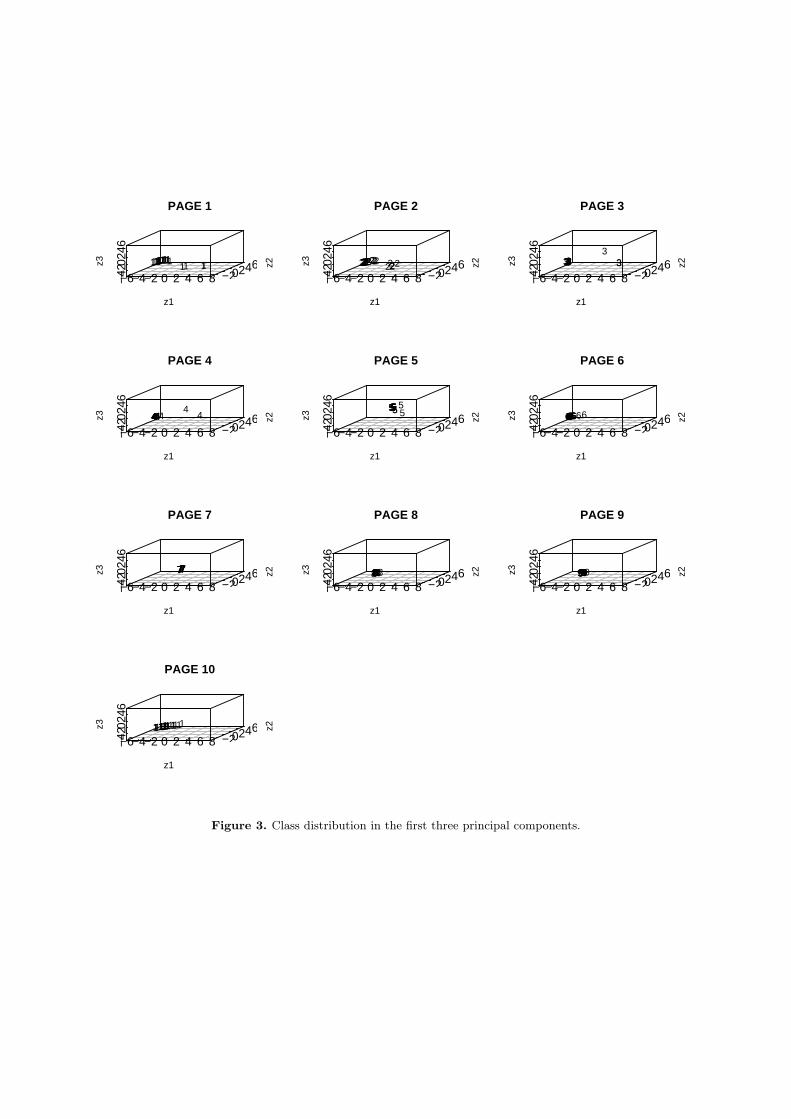
In order to visualize the distribution of the strips inside the classes, according to the features used to describethem, a Principal Component Analysis6 is performed, and the first three principal components are taken intoconsideration. In this dataset, the first three principal components retain 80% of the information (in terms ofvariance) contained in the 9 original features. The class distribution in the first three components is shown inFig. 3.

In general, from the analysis of the features space (conducted on the principal components) it can be concludedthat the different pages form in fact compact or nearly compact groups. However, some pages are not wellseparated one from the other. For example, class 8 can be confused with class 9, since the elements are close

in the features space. Indeed, the document class of the pages is the same, and their appearance in terms ofpage layout is very similar, as it is shown in Figure 4. However, note that page 7, which belongs to the samedocument class as pages 8 and 9, is better separated in the feature space. Indeed, the page layout differs fromthe latter (see Figure 4) because in page 7 there was a chapter termination.

Pages 1, 2, 3, 4 are less compact in the feature space. Indeed, pages 1 and 2 have header and footnotes, insuch a way that the strips on the right on the page have a different appearance from the rest. Pages 3 and 4have some strips at the margin which are not completely blank because there are some handwritten notes (seeFigure 4); for this reason they look very different from the other strips of the page.

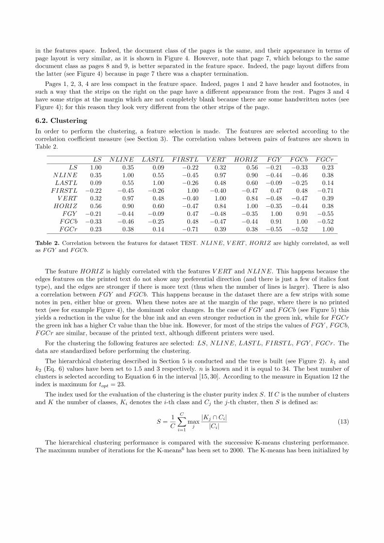
6.2. ClusteringIn order to perform the clustering, a feature selection is made. The features are selected according to thecorrelation coefficient measure (see Section 3). The correlation values between pairs of features are shown inTable 2.

LS NLINE LASTL FIRSTL V ERT HORIZ FGY FGCb FGCrLS 1.00 0.35 0.09 −0.22 0.32 0.56 −0.21 −0.33 0.23

NLINE 0.35 1.00 0.55 −0.45 0.97 0.90 −0.44 −0.46 0.38LASTL 0.09 0.55 1.00 −0.26 0.48 0.60 −0.09 −0.25 0.14

FIRSTL −0.22 −0.45 −0.26 1.00 −0.40 −0.47 0.47 0.48 −0.71V ERT 0.32 0.97 0.48 −0.40 1.00 0.84 −0.48 −0.47 0.39

HORIZ 0.56 0.90 0.60 −0.47 0.84 1.00 −0.35 −0.44 0.38FGY −0.21 −0.44 −0.09 0.47 −0.48 −0.35 1.00 0.91 −0.55

FGCb −0.33 −0.46 −0.25 0.48 −0.47 −0.44 0.91 1.00 −0.52FGCr 0.23 0.38 0.14 −0.71 0.39 0.38 −0.55 −0.52 1.00

Table 2. Correlation between the features for dataset TEST. NLINE, V ERT , HORIZ are highly correlated, as wellas FGY and FGCb.

The feature HORIZ is highly correlated with the features V ERT and NLINE. This happens because theedges features on the printed text do not show any preferential direction (and there is just a few of italics fonttype), and the edges are stronger if there is more text (thus when the number of lines is larger). There is alsoa correlation between FGY and FGCb. This happens because in the dataset there are a few strips with somenotes in pen, either blue or green. When these notes are at the margin of the page, where there is no printedtext (see for example Figure 4), the dominant color changes. In the case of FGY and FGCb (see Figure 5) thisyields a reduction in the value for the blue ink and an even stronger reduction in the green ink, while for FGCrthe green ink has a higher Cr value than the blue ink. However, for most of the strips the values of FGY , FGCb,FGCr are similar, because of the printed text, although different printers were used.

For the clustering the following features are selected: LS, NLINE, LASTL, FIRSTL, FGY , FGCr. Thedata are standardized before performing the clustering.

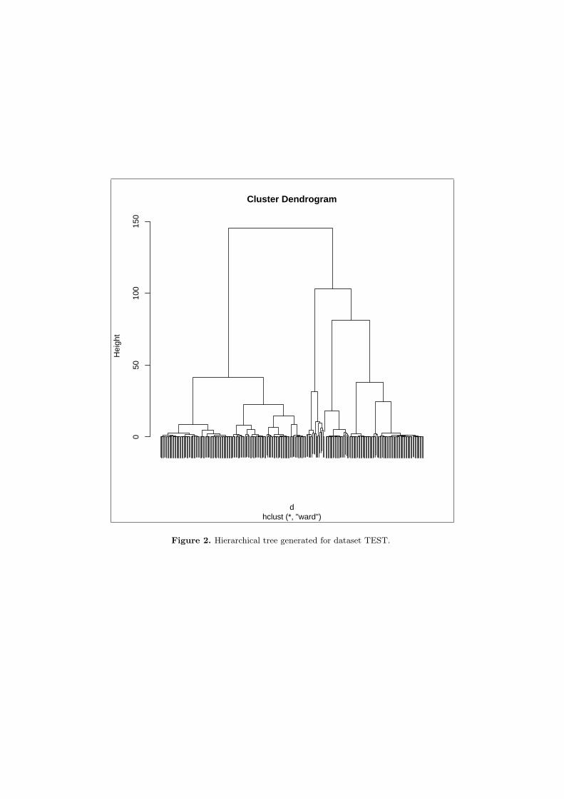
The hierarchical clustering described in Section 5 is conducted and the tree is built (see Figure 2). k1 andk2 (Eq. 6) values have been set to 1.5 and 3 respectively. n is known and it is equal to 34. The best number ofclusters is selected according to Equation 6 in the interval [15, 30]. According to the measure in Equation 12 theindex is maximum for topt = 23.

The index used for the evaluation of the clustering is the cluster purity index S. If C is the number of clustersand K the number of classes, Ki denotes the i-th class and Cj the j-th cluster, then S is defined as:

S =1C

C∑

i=1

maxj

|Kj ∩ Ci||Ci| (13)

The hierarchical clustering performance is compared with the successive K-means clustering performance.The maximum number of iterations for the K-means6 has been set to 2000. The K-means has been initialized by

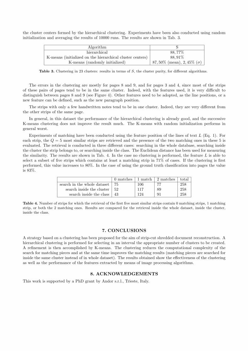
the cluster centers formed by the hierarchical clustering. Experiments have been also conducted using randominitialization and averaging the results of 10000 runs. The results are shown in Tab. 3.

Algorithm Shierarchical 88, 77%

K-means (initialized on the hierarchical cluster centers) 88, 91%K-means (randomly initialized) 87, 50% (mean), 2, 45% (σ)

Table 3. Clustering in 23 clusters: results in terms of S, the cluster purity, for different algorithms.

The errors in the clustering are mostly for pages 8 and 9, and for pages 3 and 4, since most of the stripsof these pairs of pages tend to be in the same cluster. Indeed, with the features used, it is very difficult todistinguish between pages 8 and 9 (see Figure 4). Other features need to be adopted, as the line positions, or anew feature can be defined, such as the new paragraph position.

The strips with only a few handwritten notes tend to be in one cluster. Indeed, they are very different fromthe other strips of the same page.

In general, in this dataset the performance of the hierarchical clustering is already good, and the successiveK-means clustering does not improve the result much. The K-means with random initialization performs ingeneral worst.

Experiments of matching have been conducted using the feature position of the lines of text L (Eq. 1). Foreach strip, the Q = 5 most similar strips are retrieved and the presence of the two matching ones in these 5 isevaluated. The retrieval is conducted in three different cases: searching in the whole database, searching insidethe cluster the strip belongs to, or searching inside the class. The Euclidean distance has been used for measuringthe similarity. The results are shown in Tab. 4. In the case no clustering is performed, the feature L is able toselect a subset of five strips which contains at least a matching strip in 71% of cases. If the clustering is firstperformed, this value increases to 80%. In the case of using the ground truth classification into pages the valueis 83%.

0 matches 1 match 2 matches totalsearch in the whole dataset 75 106 77 258

search inside the cluster 52 117 89 258search inside the class 43 124 91 258

Table 4. Number of strips for which the retrieval of the first five most similar strips contain 0 matching strips, 1 matchingstrip, or both the 2 matching ones. Results are compared for the retrieval inside the whole dataset, inside the cluster,inside the class.

7. CONCLUSIONS

A strategy based on a clustering has been proposed for the aim of strip-cut shredded document reconstruction. Ahierarchical clustering is performed for selecting in an interval the appropriate number of clusters to be created.A refinement is then accomplished by K-means. The clustering reduces the computational complexity of thesearch for matching pieces and at the same time improves the matching results (matching pieces are searched forinside the same cluster instead of in whole dataset). The results obtained show the effectiveness of the clusteringas well as the performance of the features extracted by means of image processing algorithms.

8. ACKNOWLEDGEMENTS

This work is supported by a PhD grant by Andor s.r.l., Trieste, Italy.

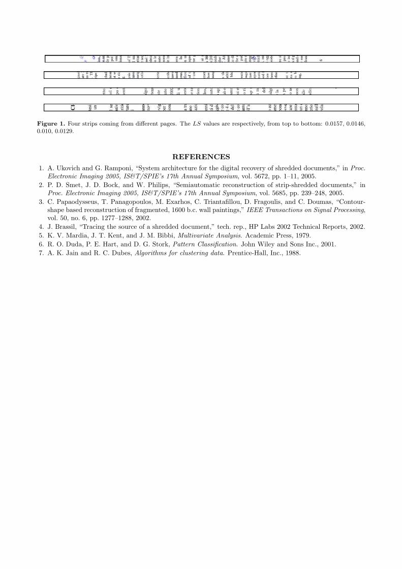
Figure 1. Four strips coming from different pages. The LS values are respectively, from top to bottom: 0.0157, 0.0146,0.010, 0.0129.

REFERENCES1. A. Ukovich and G. Ramponi, “System architecture for the digital recovery of shredded documents,” in Proc.

Electronic Imaging 2005, IS&T/SPIE’s 17th Annual Symposium, vol. 5672, pp. 1–11, 2005.2. P. D. Smet, J. D. Bock, and W. Philips, “Semiautomatic reconstruction of strip-shredded documents,” in

Proc. Electronic Imaging 2005, IS&T/SPIE’s 17th Annual Symposium, vol. 5685, pp. 239–248, 2005.3. C. Papaodysseus, T. Panagopoulos, M. Exarhos, C. Triantafillou, D. Fragoulis, and C. Doumas, “Contour-

shape based reconstruction of fragmented, 1600 b.c. wall paintings,” IEEE Transactions on Signal Processing,vol. 50, no. 6, pp. 1277–1288, 2002.

4. J. Brassil, “Tracing the source of a shredded document,” tech. rep., HP Labs 2002 Technical Reports, 2002.5. K. V. Mardia, J. T. Kent, and J. M. Bibbi, Multivariate Analysis. Academic Press, 1979.6. R. O. Duda, P. E. Hart, and D. G. Stork, Pattern Classification. John Wiley and Sons Inc., 2001.7. A. K. Jain and R. C. Dubes, Algorithms for clustering data. Prentice-Hall, Inc., 1988.

050

100

150

Cluster Dendrogram

hclust (*, "ward")d

Hei

ght

Figure 2. Hierarchical tree generated for dataset TEST.

PAGE 1

−6−4−2 0 2 4 6 8−4−2 0

2 4 6

−2 0 2 4 6 8

z1

z2z3 11111111111111111111111111111 11

PAGE 2

−6−4−2 0 2 4 6 8−4−2 0

2 4 6

−2 0 2 4 6 8

z1

z2z3 2222222 2222222222222222 2222

PAGE 3

−6−4−2 0 2 4 6 8−4−2 0

2 4 6

−2 0 2 4 6 8

z1

z2z3

3333333333333333333333

PAGE 4

−6−4−2 0 2 4 6 8−4−2 0

2 4 6

−2 0 2 4 6 8

z1

z2z3

444444444444444444444 4

PAGE 5

−6−4−2 0 2 4 6 8−4−2 0

2 4 6

−2 0 2 4 6 8

z1

z2z3 555555555555555555555

PAGE 6

−6−4−2 0 2 4 6 8−4−2 0

2 4 6

−2 0 2 4 6 8

z1

z2z3 6666666666666666666666666666

PAGE 7

−6−4−2 0 2 4 6 8−4−2 0

2 4 6

−2 0 2 4 6 8

z1

z2z3 7777777777777777777777

PAGE 8

−6−4−2 0 2 4 6 8−4−2 0

2 4 6

−2 0 2 4 6 8

z1

z2z3 8888888888888888888888

PAGE 9

−6−4−2 0 2 4 6 8−4−2 0

2 4 6

−2 0 2 4 6 8

z1

z2z3 9999999999999999999999

PAGE 10

−6−4−2 0 2 4 6 8−4−2 0

2 4 6

−2 0 2 4 6 8

z1

z2z3 1111111111111111111111111111

Figure 3. Class distribution in the first three principal components.

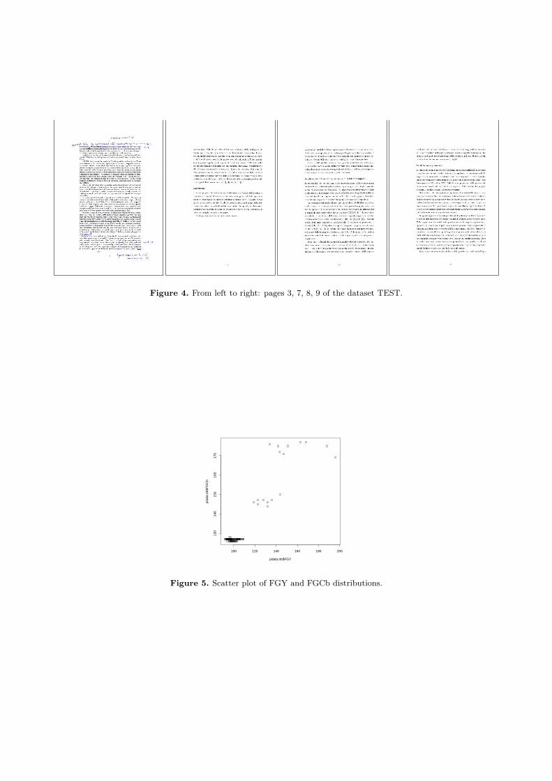
Figure 4. From left to right: pages 3, 7, 8, 9 of the dataset TEST.

100 120 140 160 180 200

130

140

150

160

170

pdata.nb$FGY

pdat

a.nb

$FG

Cb

Figure 5. Scatter plot of FGY and FGCb distributions.