Approximate best linear unbiased channel estimation for multi-antenna frequency selective channels with applications to digital TV systems

Approximate Best Linear Unbiased Channel Estimation forMulti-Antenna Frequency Selective Channels with

Applications to Digital TV systems

SerdarOzena,b, Christopher Pladdyb, S. M. Nerayanurub, Mark J. Fimoffb, and Michael D.Zoltowskic

aIzmir Institute of Technology, Dept. of Electrical & Electronics Eng., Urla,Izmir, Turkey;bZenith Electronics R&D Center, Lincolnshire, IL 60069, USA;

cPurdue University, School of ECE, West Lafayette, IN 47907, USA

ABSTRACT

We provide an iterative and a non-iterative channel impulse response (CIR) estimation algorithm for communication re-ceivers with multiple-antenna. Our algorithm is best suited for communication systems which utilize a periodically trans-mitted training sequence within a continuous stream of information symbols, and the receivers for this particular system areexpected work in a severe frequency selective multipath environment with long delay spreads relative to the length of thetraining sequence. The iterative procedure calculates the (semi-blind)Best Linear Unbiased Estimate(BLUE) of the CIR.The non-iterative version is an approximation to the BLUE CIR estimate, denoted by a-BLUE, achieving almost similarperformance, with much lower complexity. Indeed we show that, with reasonable assumptions, a-BLUE channel estimatecan be obtained by using a stored copy of a pre-computed matrix in the receiver which enables the use of the initial CIRestimate by the subsequent equalizer tap weight calculator. Simulation results are provided to demonstrate the performanceof the novel algorithms for 8-VSB ATSC Digital TV system. We also provide a simulation study of the robustness of thea-BLUE algorithm to timing and carrier phase offsets.

Keywords: channel estimation, least squares, best linear unbiased estimator, digital television, multi-antenna receivers,8-VSB

1. INTRODUCTION

For the communications systems utilizing periodically transmitted training sequence,least-squares(LS) based channelestimation or thecorrelationbased channel estimation algorithms have been the most widely used two alternatives.1 Bothmethods use a stored copy of the known transmitted training sequence at the receiver. The properties and the length ofthe training sequence are generally different depending on the particular communication system’s standard specifications.However most channel estimation schemes ignore thebaseline noiseterm which occurs due to the correlation of the storedcopy of the training sequence with the unknown symbols adjacent to transmitted training sequence, as well as the additivechannel noise.1, 2 In the sequel, we provide (semi-blind)Best Linear Unbiased Estimate(BLUE) and approximate BLUE(a-BLUE) channel estimators for communication systems using a periodically transmitted training sequence. Our novelCIR estimation algorithms can be considered assemi-blindtechniques since these methods take advantage of the statisticsof the data.3 Although the examples following the derivations of the BLUE and the a-BLUE channel estimators will bedrawn from the ATSC digital TV 8-VSB system,4 to the best of our knowledge it could be applied with minor modificationsto any digital communication system with linear modulation which employs a periodically transmitted training sequence.The novel algorithm presented in the sequel is targeted for the systems that are desired to work with channels having longdelay spreadsLd; in particular we consider the case where(NT + 1)/2 < Ld < NT , whereNT is the duration ofthe available training sequence. For instance the 8-VSB digital TV system has 728 training symbols, whereas the delayspreads of the terrestrial channels have been observed to be at least 400-500 symbols long.5, 6 The a-BLUE algorithm can

Further author information: (Send correspondence to S.O)S.O: E-mail: [email protected], Tel: +90 232 750 6510; Fax: +90 232 750 6505C.P., S.M.N., M.J.F.: E-mail:{christopher.pladdy, snerayanuru, mark.fimoff}@zenith.com, Telephone: (847) 941 8911M.D.Z: E-mail: [email protected], Telephone: (765) 494 3512

be used as an initializer to the BLUE iterations,7 or as a stand-alone alternative8 approach that produces results of nearlythe same quality as the results produced by the BLUE algorithm while at the same time requiring much less computationalcomplexity (i.e., requiring about the same number of multiplications necessary to implement ordinary least squares) andhaving storage requirements similar to that of ordinary least squares.

1.1. Overview of Generalized Least Squares

Consider the linear model

y = Ax + ν (1)

wherey is the observation (or response) vector,A is the regression (or design) matrix,x is the vector of unknown pa-rameters to be estimated, andν is the observation noise (or measurement error) vector. Assuming that it is known thatthe random noise vectorν is zero mean, and is correlated, that is Cov{ν} = Kν ≡ 1

2E{ννH} 6= σ2νI, we define the

(generalized) objective function for the model of (1) by

JGLS(x) = (y −Ax)HK−1ν (y −Ax). (2)

The least squares estimate that minimizes Equation (2) is

xgls = (AHK−1ν A)−1AHK−1

ν y, (3)

The estimator of (3) is called thebest linear unbiased estimate(BLUE)9 among alllinear unbiased estimators if the noisecovariance matrix isknownto be Cov{ν} = Kν . The estimator of (3) is called theminimum variance unbiased estimator(MVUE) amongall unbiased estimators (not only linear) if the noise isknownto beGaussianwith zero mean and withcovariance matrixKν , that isxols is called MVUE if it is known thatν ∼ N (0, Kν).

2. DATA TRANSMISSION MODEL

Let NA ≥ 1 denote the number of antennae used at the receiver. Then the baseband symbol rate sampled receive filteroutput forith antenna is given by

yi[n] ≡ yi(t)|t=nT =∑

k

Ikhi[n− k] + νi[n]

=∑

k

Ikhi[n− k] +∑

k

ηi[k]q∗[−n + k], (4)

for 1 ≤ i ≤ NA, where

Ik ={

ak, 0 ≤ k ≤ N − 1dk, N ≤ n ≤ N ′−1,

}∈A≡{α1,· · · , αM} (5)

is theM -ary complex valued transmitted sequence,A ≡ {α1,· · · , αM} ⊂C1, and{ak} ∈ C1 denote the firstN symbolswithin aframeof lengthN ′ to indicate that they are the known training symbols;νi[n] = ηi[n]∗q∗[−n] denotes the complex(colored) noise process after the (pulse) matched filter, withηi[n] being a zero-mean white Gaussian noise process withvarianceσ2

ηiper real and imaginary part;hi(t) is the complex valued impulse response of the composite channel seen by

the ith antenna including pulse shaping transmit filterq(t), the physical channel impulse responseci(t), and the receivefilter q∗(−t), and is given by

hi(t) = q(t) ∗ ci(t) ∗ q∗(−t) =L∑

k=−K

ci,kp(t− τi,k), (6)

with p(t) = q(t) ∗ q∗(−t) is the convolution of the transmit and receive filters whereq(t) has a finite support of[−Tq/2, Tq/2], and the span of the transmit and receive filters, is an even multiple of the symbol period,T ; that isTq = NqT , Nq = 2Lq ∈ Z+. {ci,k} ⊂ C1 denote complex valued physical channel gains, and{τi,k} denote the

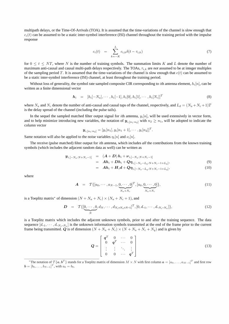
multipath delays, or the Time-Of-Arrivals (TOA). It is assumed that the time-variations of the channel is slow enough thatci(t) can be assumed to be a static inter-symbol interference (ISI) channel throughout the training period with the impulseresponse

ci(t) =L∑

k=−K

ci,kδ(t− τi,k) (7)

for 0 ≤ t ≤ NT , whereN is the number of training symbols. The summation limitsK andL denote the number ofmaximum anti-causal and causal multi-path delays respectively. The TOAs,τi,k arenotassumed to be at integer multiplesof the sampling periodT . It is assumed that the time-variations of the channel is slow enough thatc(t) can be assumed tobe a static inter-symbol interference (ISI) channel, at least throughout the training period.

Without loss of generality, the symbol rate sampled composite CIR corresponding toith antenna element,hi[n], can bewritten as a finite dimensional vector

hi = [hi[−Na], · · · , hi[−1], hi[0], hi[1], · · · , hi[Nc]]T (8)

whereNa andNc denote the number of anti-causal and causal taps of the channel, respectively, andLd = (Na +Nc +1)Tis the delay spread of the channel (including the pulse tails).

In the sequel the sampled matched filter output signal forith antenna,yi[n], will be used extensively in vector form,and to help minimize introducing new variables, the notation ofyi,[n1:n2] with n2 ≥ n1, will be adopted to indicate thecolumn vector

yi,[n1:n2] = [yi[n1], yi[n1 + 1], · · · , yi[n2]]T .

Same notation will also be applied to the noise variablesηi[n] andνi[n].

The receive (pulse matched) filter output forith antenna, which includesall the contributions from the known trainingsymbols (which includes the adjacent random data as well) can be written as

yi,[−Na:N+Nc−1] = (A + D)hi + νi,[−Na:N+Nc−1]

= Ahi + Dhi + Qηi,[−Na−Lq :N+Nc−1+Lq ], (9)

= Ahi + Hid + Qηi,[−Na−Lq :N+Nc−1+Lq ], (10)

where

A = T {[a0, · · · , aN−1, 0, · · · , 0︸ ︷︷ ︸Na+Nc

]T , [a0, 0, · · · , 0︸ ︷︷ ︸Na+Nc

]}, (11)

is a Toeplitz matrix∗ of dimension(N + Na + Nc)× (Na + Nc + 1), and

D = T {[0, · · · , 0︸ ︷︷ ︸N

, dN , · · · , dNc+Na+N−1]T , [0, d−1, · · · , d−Nc−Na ]}, (12)

is a Toeplitz matrix which includes the adjacent unknown symbols, prior to and after the training sequence. The datasequence[d−1, · · · , d−Nc−Na ] is the unknown information symbols transmitted at the end of the frame prior to the currentframe being transmitted.Q is of dimension(N + Na + Nc)× (N + Na + Nc + Nq) and is given by

Q =

qT 0 · · · 00 qT · · · 0...

.... ..

...0 0 · · · qT

(13)

∗The notation ofT {a, bT } stands for a Toeplitz matrix of dimensionM ×N with first columna = [a0, . . . , aM−1]T and first row

b = [b0, . . . , bN−1]T , with a0 = b0.

andq = [q[+Lq], · · · , q[0], · · · , q[−Lq]]T , and

Hi = HiST , (14)

hi = [hi[Nc], · · · , hi[1], hi[0], hi[−1], · · · , hi[−Na]]T = Jhi, (15)

J =

0 · · · 0 10 · · · 1 0...

......

1 0 · · · 0

(Na+Nc+1)×(Na+Nc+1)

(16)

Hi =

hTi 0 · · · 00 h

Ti · · · 0

......

. .....

0 0 · · · hTi

(N+Nc+Na)×(N+2(Na+Nc))

, (17)

andd = Sd, or equivalentlyd = ST d, where

d = [d−Nc−Na, · · ·, d−1,01×N , dN , · · ·, dN+Nc+Na−1]T (18)

d = [d−N−Na , · · · , d−1, dN , · · · , dN+Nc+Na−1]T (19)

S =[

INa+Nc 0(Na+Nc)×N 0(Na+Nc)

0(Na+Nc) 0(Na+Nc)×N INa+Nc

]. (20)

wherehi is the time reversed version ofhi (re-ordering is accomplished by the permutation matrixJ ), andHi is ofdimension(N + Na + Nc) × (2(Nc+Na)) with a “hole” inside which is created by the selection matrixS, whereS is(2(Nc+Na))× (N +2(Na+Nc)) dimensionalselectionmatrix which retains the random data, eliminates theN zeros inthe middle of the vectord.

By defining

h = [hT1 , · · · , hT

NA]T , (21)

y = [yT1,[−Na:N+Nc−1], · · · ,yT

NA,[−Na:N+Nc−1]]T , (22)

η = [ηT1,[−Na−Lq :N+Nc−1+Lq ], · · · ,ηT

NA,[−Na−Lq :N+Nc−1+Lq ]]T (23)

and using Equations (8) and (10) we obtain

y = Ah + Hd + Qη (24)

where

A = INA⊗A, (25)

H =[HT

1 , · · · , HTNA

]T

, (26)

Q = INA⊗Q, (27)

andINAis NA dimensional identity matrix,⊗ denotes the Kronecker matrix product.

2.1. Receiver Antenna Array Geometry

For a receiver employing an antenna array we will make the basic assumption that every multipath reflection reaches all theantenna elements at the same time but with different phase angles. This assumption enables us to drop the antenna indexfrom the TOA’s; that is in the sequel we will useτi,k = τk for −K ≤ k ≤ L.

Plane wavephase frontincident onAntenna 1

Plane wave

Plane wave NORMAL

Plane wavephase frontincident onAntenna 2

Direction of propagation ofplane wave

Antenna 1

Antenna 2

Antenna 1 Antenna 2

(a)

(b)

θ

φ

y

∆

x

θ θ

y

d=

∆co

sθsin

φ

x

z

∆

Figure 1. (a) Antenna geometry used to determine the Direction-Of-Arrival (DOA) of a plane wave incident on a two element lineararray oriented alongx-axis. (b) Baseband model of a linear array oriented along thex-axis receiving a plane wave from direction{θ, φ}.

In the sequel we provide a brief derivation of the phase difference in the multipath components at each antenna element.Considering Figure 1 it is straightforward to show that the distanced that the plane wave which is on the second antennahas to travel to reach the first antenna is given by

d = ∆ cos θ sin φ (28)

where∆ is inter-element spacing,θ is the angle between the projection of the plane-wave normal onto thex-y plane andthex-axis,φ is the angle between the plane-wave normal and thez-axis. The angle tuple{θ, φ} is called the Direction-Of-Arrival (DOA). Then the phase difference,ψ(∆, θ, φ, λo), between the signal component on array element antenna twoand the reference antenna one is

ψ =2πd

λo=

2π∆ cos θ sin φ

λo=

2πfo∆ cos θ sin φ

c, (29)

whereλo = c/fo is the transmission wavelength,c is the speed of the light,3× 108 m/s,fo is the transmission frequencyin Hz. Most often the inter-element spacing∆ is taken to be multiple of wavelengthλo, that is

∆ = mλo, m ∈ R+. (30)

Then Equation (29) can be written as

ψ = 2πm cos θ sin φ (31)

wherem is expressed in terms of wavelengths.

Without loss of generality, we let the antenna number one, with the physical channel complex gains coefficientsc1 =[c1,−K , · · · , c1,0, · · · , c1,L]T , to be the reference antenna. Then the complex valued gainsci,k for remaining antennae canbe given by

ci,k = ui(θk, φk)c1,k, 2 ≤ i ≤ NA,−K ≤ k ≤ L, (32)

whereui(θk, φk) = e−j(i−1)ψ(θk,φk). Substituting Equation (32) into (6) the composite channel impulse responses for theremaining antennae are written as

hi(t) =L∑

k=−K

ui(θk, φk)c1,kp(t− τk), 2 ≤ i ≤ NA, (33)

where in the case of auniform linear arrayof NA identical antennas, with identical inter-element spacing∆, and theplane-wave assumption holds, thearray manifold

u(θk, φk) = [u1(θk, φk), u2(θk, φk), · · · , uNA(θk, φk)]T

has the form10

u(θk, φk) = [1, e−jψ(θk,φk), · · · , e−j(NA−1)ψ(θk,φk)]T (34)

whereψ(θk, φk) = 2πm cos θk sin φk and m ∈ R+ is specified in terms of wavelengths. Combining Equations (4)and (33) the received signal at the output of receive filter,y[n] = [y1[n], y2[n], · · · , yNA

[n]]T , in vector form is given by

y[n] =

(∑

k

L∑

l=−K

Iku(θl, φl)c1,lp(t− τl)

)∣∣∣∣∣t=nT

+ ν[n], (35)

whereν[n] = [ν1[n], · · · , νNA [n]]T .

3. OVERVIEW OF THE BLUE CIR ESTIMATOR

For comparison purposes we first provide the well known correlation and ordinary least squares based estimators, wherecorrelations based estimation is denotedhu (the subscriptu stands for theuncleanedCIR estimate) and is given by

hu =1

ra[0]A

Hy, (36)

with ra[0] =N−1∑k=0

‖ak‖2, and the ordinary least squares CIR estimate is denoted byhc (the subscriptc stands for the

cleanedCIR estimate) and is given by

hc = (AH

A)−1AH

y, (37)

where “cleaning” is accomplished by removing the known sidelobes of the aperiodic correlation operation as accomplishedin (36).

We can denote the two terms on the right side of Equation (10) byv = Hd + Qη. Hence we rewrite (24) as

y = Ah + v. (38)

By noting the statistical independence of the random vectorsd andη, and also noting that both vectors are zero mean, thecovariance matrix,Kv of v is given by

Cov{v} = Kv ≡ 12E{vvH} =

Ed

2HH

H+ Kη, (39)

whereEd is the energy of the transmitted information symbols, and equals to21 if the symbols{dk} are chosen from theset{±1,±3,±5,±7}. Kη is the covariance of the noise vector and is given by

Kη =

{σ2

ηQQH

, if noise powers are identical on all diversity branchesdiag{σ2

η1QQH , · · · , σ2

ηNAQQH}, if noise powers are different,

(40)

where diag{} creates diagonal matrix by placing the entries inside the curly brackets along the main diagonal.

For the model of (38) the generalized least squares objective function to be minimized is

JGLS(h) =(y − Ah

)H

K−1v

(y − Ah

). (41)

Then the generalized least-squares solution to the model of Equation (38) which minimizes the objective function ofJGLS(h)is given by

hK = (AH

K−1v A)−1A

HK−1

v y. (42)

The problem with Equation (42) is that the channel estimatehK is based on the covariance matrixKv, which is a functionof the true channel impulse response vectorh as well as the channel noise varianceσ2

ηi. In actual applications the BLUE

channel estimate of Equation (42) can not be exactly obtained. Hence we need aniterative technique to calculate general-ized least squares estimate of (42) where every iteration produces an updated estimate of the covariance matrix as well asthe noise variance. Without going into the details, a simplified version of the iterations, which yield a closer approximationto the exact BLUE CIR estimate after each step, is provided in Algorithm 1. In the intermediate steps noise variance foreach antenna is estimated by

σ2ηi

=1

2Eq(N −Na −Nc)‖yi,[Nc:N−Na] − yi,[Nc:N−Na]‖2,

whereEq = ‖q‖2 andyi,[Nc:N−Na] = Ahi,th,

andA = T {[aNc+Na , · · ·, aN−1]T , [aNc+Na , · · ·, a0]

}. For further details regarding the BLUE algorithm, the readers are

referred to the publication by Pladdy7 et al. For details regarding the thresholding algorithms we refer the readers toOzen8

et al.

Algorithm 1 Iterative Algorithm to obtain a CIR estimate via Generalized Least-Squares

[1] Get an initial CIR estimate using one of (36) or (37), and denote it byh[0];

[2] Threshold the initial CIR estimate, and denote it byh(th)

[0];

[3] Estimate the noise variance on all diversity branchesσ2ηi [0], and use lower part of Equation (40) to obtain the estimated noise

covariance matrixKη[0][4]for k = 1, . . . , Niter do

[4-a] Calculate the inverse of the (estimated) covariance matrix

K−1

v [k] =

[Ed

2H(h

(th)[k − 1])H

H(h

(th)[k − 1]) + Kη[k − 1]

]−1

;

[4-b] hK [k] = (AH

K−1

v [k]A)−1AH

K−1

v [k]y;

[4-c] Threshold the CIR estimatehK [k], and denote it byh(th)

[k];

[4-d] Estimate the noise variance on all diversity branchesσ2ηi [k], and use lower part of Equation (40) to obtain the estimated

noise covariance matrixKη[k].end for

3.1. Approximate BLUE CIR estimation

An alternative approach may be used to produce results of nearly the same quality as the results produced by the algorithmdescribed in Algorithm 1 while at the same time requiring much less computational complexity (i.e., requiring about thesame number of multiplications necessary to implement Equation (37)) and having storage requirements similar to thatof Equation (37). According to this alternative, the initial least squares estimation error can be reduced by seeking an

approximation in which it is assumed that the baseband representation of the physical channelci(t) is a distortion-free (nomultipath) channel; that is

ci(t) = δ(t) (43)

which implies

hi(t) = p(t) ∗ ci(t) = pi(t). (44)

Thus we can assume that our finite length channel impulse response vector can be (initially) approximated by

hi = [0,· · · ,0︸ ︷︷ ︸Na−Nq

, p[−Nq],· · · , p[0],· · · , p[Nq]︸ ︷︷ ︸raised cosine pulse

, 0,· · · , 0︸ ︷︷ ︸Nc−Nq

]T (45)

with the assumptions ofNa ≥ Nq andNc ≥ Nq, that is the tail span of the composite pulse shape is well confined to withinthe assumed delay spread of[−NaT, NcT ]. The assumption of (45) is assumed to be valid fori = 1, 2, . . . , NA. Thenthe approximation of (45) can be substituted into Equations (16-17) to yield an initial (approximate) channel convolution

matrix Hi and is given byHi = HiST whereHi is formed as in Equation (17) withhi = Jhi. We can also assume a

reasonable received Signal-to-Noise (SNR) ratio measured at the input to the matched filter which is given by

SNR =Ed ‖(c(t) ∗ q(t))|t=nT ‖2

σ2η

=Ed ‖q‖2

σ2η

. (46)

For instance we can assume an approximateSNR of 20dB yielding an initial noise variance of

σ2η =

Ed‖q‖2100

. (47)

All diversity branches are assumed to have the same noise power in Equation (47). Then we can obtain the approximatetwo antenna multi-antenna convolution matrixH of Equation (26) by appendingHi matrices, and by usingσ2

η we canpre-calculate the initial approximate covariance matrix where the covariance matrix of the approximate channel is given by

Kv(H) =12EdHH

H+ σ2

ηQQH

, (48)

which further leads to the initial channel estimate of

hK =(A

H[Kv(H)]−1A

)−1

AH

[Kv(H)]−1

︸ ︷︷ ︸pre-computed and stored

y. (49)

Equation (49) is the resulting a-BLUE CIR estimate. The key advantage of the a-BLUE is that the matrix

(A

H[Kv(H)]−1A

)−1

AH

[Kv(H)]−1

is constructed based on the initial assumptions that the receiver is expected to operate, and can bepre-computedandstored

in the receiver. By pre-computing and storing the matrix(A

H[Kv(H)]−1A

)−1

AH

[Kv(H)]−1 as in Equation (49) we

obtain a CIR estimate with much lower computational complexity than the BLUE algorithm. We also note that a-BLUECIR estimate can be used either as a stand-alone CIR estimator, or an initial estimate which can be used by the BLUEalgorithm; additionally it can be used as an initial CIR estimate to be used in the calculation of the tap weights of asubsequent equalizer.

However, there is one problem with the covariance matrix of the approximate (assumed) channel. As an exampleconsider a simple two antenna case where we approximate bothh1 andh2 as

h1 = h2 = [0,· · · ,0︸ ︷︷ ︸Na−Nq

, p[−Nq],· · · , p[0],· · · , p[Nq]︸ ︷︷ ︸raised cosine pulse

, 0,· · · , 0︸ ︷︷ ︸Nc−Nq

]T . (50)

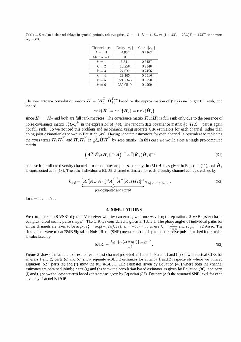
Table 1.Simulated channel delays in symbol periods, relative gains.L = −1, K = 6, Ld ≈ (1 + 333 + 2Nq)T = 453T ≈ 44µsec,Nq = 60.

Channel taps Delay{τk} Gain{|ck|}k = −1 -0.957 0.7263

Main k = 0 0 1k = 1 3.551 0.6457k = 2 15.250 0.9848k = 3 24.032 0.7456k = 4 29.165 0.8616k = 5 221.2345 0.6150k = 6 332.9810 0.4900

The two antenna convolution matrixH = [HT

1 , HT

2 ]T based on the approximation of (50) is no longer full rank, andindeed

rank{H} = rank{H1} = rank{H2}sinceH1 = H2 and both are full rank matrices. The covariance matrixKv(H) is full rank only due to the presence of

noise covariance matrixσ2ηQQ

Hin the expression of (48). The random data covariance matrix1

2EdHHH

part is againnot full rank. So we noticed this problem and recommend using separate CIR estimators for each channel, rather thandoing joint estimation as shown in Equation (49). Having separate estimators for each channel is equivalent to replacing

the cross termsH1HH

2 andH2HH

1 in 12EdHH

Hby zero matrix. In this case we would store a single pre-computed

matrix(AH [Kv(H1)]−1A

)−1

AH [Kv(H1)]−1 (51)

and use it for all the diversity channels’ matched filter outputs separately. In (51)A is as given in Equation (11), andH1

is constructed as in (14). Then the individual a-BLUE channel estimates for each diversity channel can be obtained by

hi,K =(AH[Kv(H1)]−1A

)−1

AH [Kv(H1)]−1

︸ ︷︷ ︸pre-computed and stored

yi,[−Na:N+Nc−1], (52)

for i = 1, . . . , NA.

4. SIMULATIONS

We considered an 8-VSB4 digital TV receiver with two antennas, with one wavelength separation. 8-VSB system has acomplex raised cosine pulse shape.4 The CIR we considered is given in Table 1. The phase angles of individual paths forall the channels are taken to bearg{ck} = exp(−j2πfcτk), k = −1, · · · , 6 wherefc = 50

TsymandTsym = 92.9nsec. The

simulations were run at 28dB Signal-to-Noise-Ratio (SNR) measured at the input to the receive pulse matched filter, and itis calculated by

SNRi =Ed ‖{ci(t) ∗ q(t)}t=kT ‖2

σ2ηi

. (53)

Figure 2 shows the simulation results for the test channel provided in Table 1. Parts (a) and (b) show the actual CIRs forantenna 1 and 2; parts (c) and (d) show separate a-BLUE estimates for antenna 1 and 2 respectively where we utilizedEquation (52); parts (e) and (f) show the full a-BLUE CIR estimates given by Equation (49) where both the channelestimates are obtained jointly; parts (g) and (h) show the correlation based estimates as given by Equation (36); and parts(i) and (j) show the least squares based estimates as given by Equation (37). For part (c-f) the assumed SNR level for eachdiversity channel is 19dB.

We also note that the iterative BLUE CIR estimation algorithm is very powerful but computationally very demanding,thus in many applications the approximate BLUE, as shown in parts (e-f), could be sufficiently acceptable as an initialestimate. The performance measure is the normalized least-squares error which is defined by

ENLS =‖hi − hi‖2

Na + Nc + 1, (54)

for i = 1, . . . , NA. Approximate BLUE significantly outperforms the correlation and ordinary least squares based CIRestimation algorithms, but it has virtually identical computational complexity and storage requirement.

0 100 200 300 400−0.4

−0.2

0

0.2

0.4

0.6

Real part of the CIR1

0 100 200 300 400

−0.2

0

0.2

0.4

0.6

Real part of the CIR2

0 100 200 300 400

−0.4

−0.2

0

0.2

0.4

0.6

Real Part of simpler aBLUE for Channel 1

NLSE=0.00019167

0 100 200 300 400

−0.2

0

0.2

0.4

0.6

Real Part of simpler aBLUE for Channel 1

NLSE=0.00014917

0 100 200 300 400

−0.4

−0.2

0

0.2

0.4

0.6

Real Part of Full aBLUE for Channel 1

NLSE=0.00043068

0 100 200 300 400

−0.2

0

0.2

0.4

0.6

Real Part of Full aBLUE for Channel 2

NLSE=0.00029803

0 100 200 300 400−0.4

−0.2

0

0.2

0.4

0.6

Real Part of Correlation Estimate for Channel 1

NLSE=0.002966

0 100 200 300 400−0.4

−0.2

0

0.2

0.4

0.6

Real Part of Correlation Estimate for Channel 2

NLSE=0.0027185

0 100 200 300 400

−0.4

−0.2

0

0.2

0.4

0.6

Real Part of Least Squares Estimate for Channel 1

NLSE=0.0010994

0 100 200 300 400

−0.2

0

0.2

0.4

0.6

Real Part of Least Squares Estimate for Channel 2

NLSE=0.00089472

(a) (b)

(c) (d)

(e) (f)

(g) (h)

(i) (j)

Figure 2. Parts (a) and (b) show the actual CIRs for antenna 1 and 2; parts (c) and (d) show separate a-BLUE estimates for antenna 1and 2 respectively where we utilized Equation (52); parts (e) and (f) show the full a-BLUE CIR estimates given by Equation (49) whereboth the channel estimates are obtained jointly; parts (g) and (h) show the correlation based estimates as given by Equation (36); andparts (i) and (j) show the least squares based estimates as given by Equation (37). For part (c-f) the assumed SNR level for each diversitychannel is 19dB.

4.1. Robustness of the a-BLUE Algorithm to Timing and Carrier Offsets

The robustness of the a-BLUE CIR estimator to (clock) timing offset and carrier phase offset has also been studied forthe single antenna receiver. Theassumedchannel impulse response shown in Equation (45) consists of perfectly sampledcomposite pulse shape appearing in the middle of the CIR vector. One may want to investigate the effect of having areceiver timing offset and/or the carrier phase offset on the a-BLUE algorithm.

For timing offset simulations the CIR’s are created as

hto = [0, · · · , 0︸ ︷︷ ︸Na−Nq

, p[−Nq+εto], · · · , p[−1+εto], p[εto], p[1+εto], · · · , p[Nq+εto], 0, · · · , 0︸ ︷︷ ︸Nc−Nq

]T (55)

whereεto ∈ (−T2 , T

2 ] is the timing offset. Then for the channel of (55) with a fixedεto ∈ (−T2 , T

2 ], we estimated the CIRusing Equation (49), and calculated the least squares estimation errorENLS between the actual CIR and the estimated CIR.

Similarly, for carrier phase offset simulations the CIR’s are created as

hco = εco[0, · · · , 0︸ ︷︷ ︸Na−Nq

, p[−Nq], · · · , p[−1], p[0], p[1], · · · , p[Nq], 0, · · · , 0︸ ︷︷ ︸Nc−Nq

]T (56)

whereεco = exp(−j2πθ) is the unit complex vector that rotates the original CIR with respect to the offset angleθ ∈(−π, π]. Then for the channel of (56) with a fixedεco, we estimated the CIR using Equation (49), and calculated the leastsquares estimation errorENLS between the actual CIR and the estimated CIR.

The results obtained by varying the timing offsetεto, and the carrier offsetεco are provided in Figure 3 parts (a) and (b)respectively. As can be seen in Figure 3 parts (a) there is a slight degradation in the resulting CIR estimate due to timingoffset which is normally expected; however a-BLUE algorithm is insensitive to carrier phase offset. Both figures show therobustness of the a-BLUE algorithm to timing and carrier phase offsets.

−0.5 T −0.4 T −0.3 T −0.2 T −0.1 T 0 0.1 T 0.2 T 0.3 T 0.4 T 0.5 T2

2.5

3

3.5

4

4.5x 10

−7 Effect of timing offset on a−BLUE

Timing offset in fractions of the symbol period T, [−T/2, T/2]

−pi −0.8*pi −0.6*pi −0.4*pi −0.2*pi 0 0.2*pi 0.4*pi 0.6*pi 0.8*pi pi 2.1933

2.1933

2.1933

2.1933

2.1933

2.1933

2.1933x 10

−7 Effect of carrier offset on a−BLUE

Carrier phase offset in radians, [−π, π ]

LS E

rror

(C

ompa

red

to th

e ac

tual

CIR

with

offs

et)

(a)

(b)

Figure 3. Simulation results showing the robustness of the a-BLUE algorithm to (a) timing offset, and (b) carrier recovery phase offset.

5. CONCLUSION

This paper demonstrates the BLUE and a-BLUE CIR estimation algorithms for channels with long delay spreads, wherethe number of training symbols can be insufficient to support the length of the channel. In particular we show that a-BLUEinitial channel estimation algorithm outperforms the standard least squares and correlation based initial channel estimationalgorithms achieving the same computational complexity. This feature makes the a-BLUE algorithm an attractive choicefor receivers employing channel estimate based (indirect) equalizers,6 or for receivers with direct adaptive equalizerswhere a quick and reliable channel information is needed for equalizer tap weight initialization.

We also demonstrated the robustness of the a-BLUE algorithm to timing and carrier offsets when there is no multipathpresent.

Acknowledgments

This research was funded in part by the NSF under grant number CCR0118842 and by Zenith Electronics Corporation.

REFERENCES

1. H. Arslan, G. E. Bottomley, “Channel estimation in narrowband wireless communication systems,” Wireless Comuni-cations and Mobile Computing, vol. 1, pp. 201-219, 2001.

2. H-K Song, “A channel estimation using sliding window aproach and tuning algorithm for MLSE,” IEEE Communica-tions Letters, vol. 3, pp. 211-213, 1999.

3. E. de Carvalho, D. Slock, “Semi-blind methods for FIR multi-channel estimation,” Chapter 7 inSignal ProcessingAdvances in Wireless and Mobile Communications; Trends in Channel Estimation and Equalization, G. Giannakis, Y.Hua, P. Stoica, L. Tong, vol. 1, Prentice-Hall, 2001

4. ATSC Digital Television Standard, A/53, September 1995. (available from http://www.atsc.org/standards.html )5. S.Ozen, M. D. Zoltowski, M. Fimoff, “A Novel Channel Estimation Method: Blending Correlation and Least-Squares

Based Approaches,” Proceedings of ICASSP, v. 3, pp. 2281-2284, 2002.6. S.Ozen, W. Hillery, M. D. Zoltowski, S. M. Nerayanuru, M. Fimoff, “Structured Channel Estimation Based Decision

Feedback Equalizers for Sparse Multipath Channels with Applications to Digital TV Receivers,” Proceedings of theThirty-Sixth Asilomar Conference on Signals, Systems and Computers, vol. 1, pp. 558-564, November 3-6, 2002.

7. C. Pladdy, S.Ozen, M. Fimoff, S. M. Nerayanuru, M. D. Zoltowski,“Best Linear Unbiased Channel Estimation forFrequency Selective Multipath Channels with Long Delay Spreads,” accepted to be published in the Proceedings ofFall-2003Vehicular Technology Conference, Orlando, Florida, USA, October-2003.

8. S. Ozen, M. Fimoff, C. Pladdy, S. M. Nerayanuru, M. D. Zoltowski, “Approximate Best Linear Unbiased ChannelEstimation for Frequency Selective Multipath Channels with Long Delay Spreads,” accepted to be published in theProceedings of the Thirty-Seventh Asilomar Conference on Signals, Systems and Computers, November 2003.

9. G. A. F. Seber,Linear Regresion Analysis, John Wiley and Sons, 1977.10. R. Roy and T. Kailath, “ESPRIT-estimation of signal parameters via rotational invariance techniques,” IEEE Transac-

tions on Signal Processing, vol. 37. pp. 984-995, July 1989.