Title stata.com discrim lda postestimation ... · mahalanobis calculates the squared Mahalanobis distance between the observations and group means. If you specify the group() option,

Title stata.com

discrim lda postestimation — Postestimation tools for discrim lda

Description Syntax for predict Menu for predict Options for predictSyntax for estat Menu for estat Options for estat Remarks and examplesStored results Methods and formulas References Also see

Description

The following postestimation commands are of special interest after discrim lda:

Command Description

estat anova ANOVA summaries tableestat canontest tests of the canonical discriminant functionsestat classfunctions classification functionsestat classtable classification tableestat correlations correlation matrices and p-valuesestat covariance covariance matricesestat errorrate classification error-rate estimationestat grdistances Mahalanobis and generalized squared distances between the group

meansestat grmeans group means and variously standardized or transformed meansestat grsummarize group summariesestat list classification listingestat loadings canonical discriminant-function coefficients (loadings)estat manova MANOVA tableestat structure canonical structure matrixestat summarize estimation sample summaryloadingplot plot standardized discriminant-function loadingsscoreplot plot discriminant-function scoresscreeplot plot eigenvalues

The following standard postestimation commands are also available:

Command Description

∗estimates cataloging estimation resultspredict group classification and posterior probabilities

∗All estimates subcommands except table and stats are available; see [R] estimates.

1

2 discrim lda postestimation — Postestimation tools for discrim lda

Special-interest postestimation commands

estat anova presents a table summarizing the one-way ANOVAs for each variable in the discriminantanalysis.

estat canontest presents tests of the canonical discriminant functions. Presented are the canonicalcorrelations, eigenvalues, proportion and cumulative proportion of variance, and likelihood-ratio testsfor the number of nonzero eigenvalues.

estat classfunctions displays the classification functions.

estat correlations displays the pooled within-group correlation matrix, between-groups cor-relation matrix, total-sample correlation matrix, and/or the individual group correlation matrices.Two-tailed p-values for the correlations may also be requested.

estat covariance displays the pooled within-group covariance matrix, between-groups covariancematrix, total-sample covariance matrix, and/or the individual group covariance matrices.

estat grdistances provides Mahalanobis squared distances between the group means along withthe associated F statistics and significance levels. Also available are generalized squared distances.

estat grmeans provides group means, total-sample standardized group means, pooled within-groupstandardized means, and canonical functions evaluated at the group means.

estat loadings present the canonical discriminant-function coefficients (loadings). Unstandard-ized, pooled within-class standardized, and total-sample standardized coefficients are available.

estat manova presents the MANOVA table associated with the discriminant analysis.

estat structure presents the canonical structure matrix.

Syntax for predictpredict

[type

]newvar

[if] [

in] [

, statistic options]

predict[

type] {

stub* | newvarlist} [

if] [

in] [

, statistic options]

statistic Description

Main

classification group membership classification; the default when one variable isspecified and group() is not specified

pr probability of group membership; the default when group() isspecified or when multiple variables are specified

mahalanobis Mahalanobis squared distance between observations and groupsdscore discriminant function scoreclscore group classification function score

∗looclass leave-one-out group membership classification; may be used onlywhen one new variable is specified

∗loopr leave-one-out probability of group membership∗loomahal leave-one-out Mahalanobis squared distance between observations and

groups

discrim lda postestimation — Postestimation tools for discrim lda 3

options Description

Main

group(group) the group for which the statistic is to be calculated

Options

priors(priors) group prior probabilities; defaults to e(grouppriors)

ties(ties) how ties in classification are to be handled; defaults to e(ties)

priors Description

equal equal prior probabilitiesproportional group-size-proportional prior probabilitiesmatname row or column vector containing the group prior probabilitiesmatrix exp matrix expression providing a row or column vector of the group

prior probabilities

ties Description

missing ties in group classification produce missing valuesrandom ties in group classification are broken randomlyfirst ties in group classification are set to the first tied group

You specify one new variable with classification or looclass; either one or e(N groups) new variables withpr, loopr, mahalanobis, loomahal, or clscore; and one to e(f) new variables with dscore.

Unstarred statistics are available both in and out of sample; type predict . . . if e(sample) . . . if wanted only forthe estimation sample. Starred statistics are calculated only for the estimation sample, even when if e(sample)is not specified.

group() is not allowed with classification, dscore, or looclass.

Menu for predictStatistics > Postestimation > Predictions, residuals, etc.

Options for predict

� � �Main �

classification, the default, calculates the group classification. Only one new variable may bespecified.

pr calculates group membership posterior probabilities. If you specify the group() option, specifyone new variable. Otherwise, you must specify e(N groups) new variables.

mahalanobis calculates the squared Mahalanobis distance between the observations and groupmeans. If you specify the group() option, specify one new variable. Otherwise, you must specifye(N groups) new variables.

dscore produces the discriminant function score. Specify as many variables as leading discriminantfunctions that you wish to score. No more than e(f) variables may be specified.

4 discrim lda postestimation — Postestimation tools for discrim lda

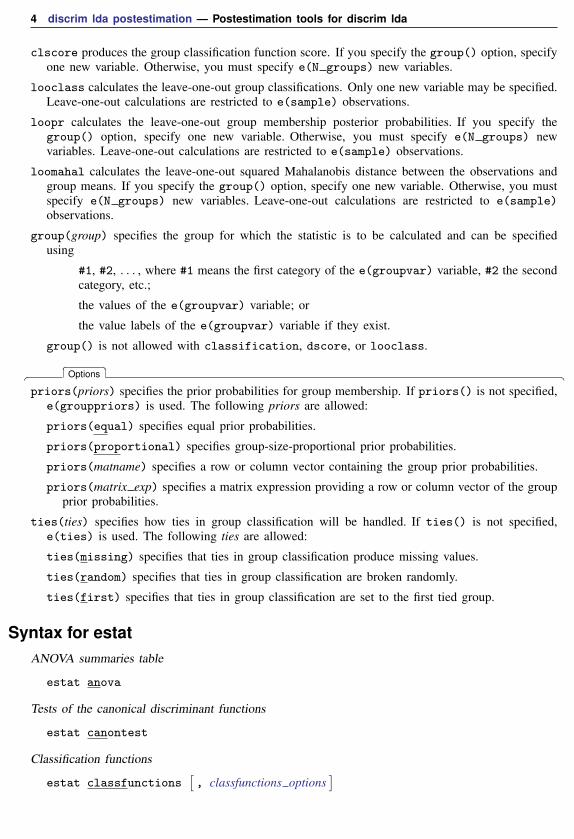
clscore produces the group classification function score. If you specify the group() option, specifyone new variable. Otherwise, you must specify e(N groups) new variables.

looclass calculates the leave-one-out group classifications. Only one new variable may be specified.Leave-one-out calculations are restricted to e(sample) observations.

loopr calculates the leave-one-out group membership posterior probabilities. If you specify thegroup() option, specify one new variable. Otherwise, you must specify e(N groups) newvariables. Leave-one-out calculations are restricted to e(sample) observations.

loomahal calculates the leave-one-out squared Mahalanobis distance between the observations andgroup means. If you specify the group() option, specify one new variable. Otherwise, you mustspecify e(N groups) new variables. Leave-one-out calculations are restricted to e(sample)observations.

group(group) specifies the group for which the statistic is to be calculated and can be specifiedusing

#1, #2, . . . , where #1 means the first category of the e(groupvar) variable, #2 the secondcategory, etc.;

the values of the e(groupvar) variable; or

the value labels of the e(groupvar) variable if they exist.

group() is not allowed with classification, dscore, or looclass.

� � �Options �

priors(priors) specifies the prior probabilities for group membership. If priors() is not specified,e(grouppriors) is used. The following priors are allowed:

priors(equal) specifies equal prior probabilities.

priors(proportional) specifies group-size-proportional prior probabilities.

priors(matname) specifies a row or column vector containing the group prior probabilities.

priors(matrix exp) specifies a matrix expression providing a row or column vector of the groupprior probabilities.

ties(ties) specifies how ties in group classification will be handled. If ties() is not specified,e(ties) is used. The following ties are allowed:

ties(missing) specifies that ties in group classification produce missing values.

ties(random) specifies that ties in group classification are broken randomly.

ties(first) specifies that ties in group classification are set to the first tied group.

Syntax for estatANOVA summaries table

estat anova

Tests of the canonical discriminant functions

estat canontest

Classification functions

estat classfunctions[, classfunctions options

]

discrim lda postestimation — Postestimation tools for discrim lda 5

Correlation matrices and p-values

estat correlations[, correlations options

]Covariance matrices

estat covariance[, covariance options

]Mahalanobis and generalized squared distances between the group means

estat grdistances[, grdistances options

]Group means and variously standardized or transformed means

estat grmeans[, grmeans options

]Canonical discriminant-function coefficients (loadings)

estat loadings[, loadings options

]MANOVA table

estat manova

Canonical structure matrix

estat structure[, format(% fmt)

]classfunctions options Description

Main

adjustequal adjust the constant even when priors are equalformat(% fmt) numeric display format; default is %9.0g

Options

priors(priors) group prior probabilities; defaults to e(grouppriors)

nopriors suppress display of prior probabilities

correlations options Description

Main

within display pooled within-group correlation matrix; the defaultbetween display between-groups correlation matrixtotal display total-sample correlation matrixgroups display the correlation matrix for each groupall display all the abovep display two-sided p-values for requested correlationsformat(% fmt) numeric display format; default is %9.0g

nohalf display full matrix even if symmetric

6 discrim lda postestimation — Postestimation tools for discrim lda

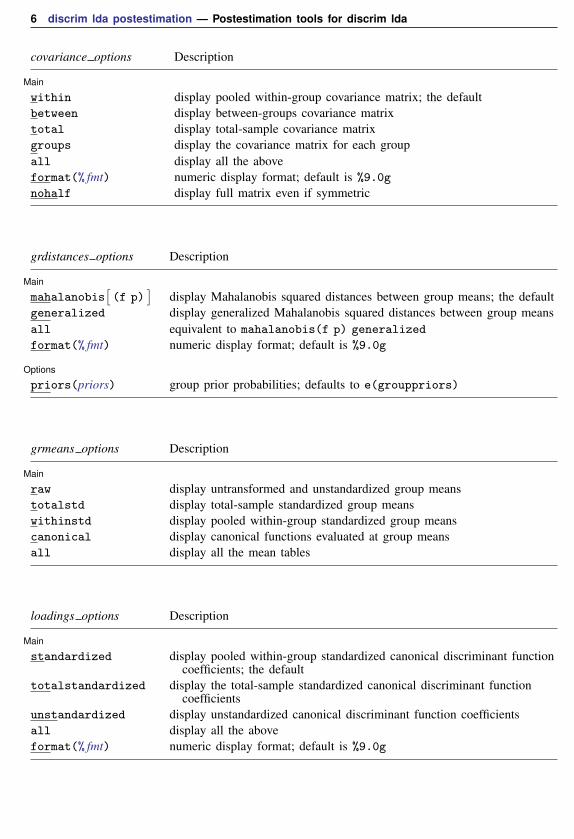
covariance options Description

Main

within display pooled within-group covariance matrix; the defaultbetween display between-groups covariance matrixtotal display total-sample covariance matrixgroups display the covariance matrix for each groupall display all the aboveformat(% fmt) numeric display format; default is %9.0g

nohalf display full matrix even if symmetric

grdistances options Description

Main

mahalanobis[(f p)

]display Mahalanobis squared distances between group means; the default

generalized display generalized Mahalanobis squared distances between group meansall equivalent to mahalanobis(f p) generalized

format(% fmt) numeric display format; default is %9.0g

Options

priors(priors) group prior probabilities; defaults to e(grouppriors)

grmeans options Description

Main

raw display untransformed and unstandardized group meanstotalstd display total-sample standardized group meanswithinstd display pooled within-group standardized group meanscanonical display canonical functions evaluated at group meansall display all the mean tables

loadings options Description

Main

standardized display pooled within-group standardized canonical discriminant functioncoefficients; the default

totalstandardized display the total-sample standardized canonical discriminant functioncoefficients

unstandardized display unstandardized canonical discriminant function coefficientsall display all the aboveformat(% fmt) numeric display format; default is %9.0g

discrim lda postestimation — Postestimation tools for discrim lda 7

Menu for estatStatistics > Postestimation > Reports and statistics

Options for estatOptions for estat are presented under the following headings:

Options for estat classfunctionsOptions for estat correlationsOptions for estat covarianceOptions for estat grdistancesOptions for estat grmeansOptions for estat loadingsOption for estat structure

Options for estat classfunctions

� � �Main �

adjustequal specifies that the constant term in the classification function be adjusted for priorprobabilities even though the priors are equal. By default, equal prior probabilities are not used inadjusting the constant term. adjustequal has no effect with unequal prior probabilities.

format(% fmt) specifies the matrix display format. The default is format(%9.0g).

� � �Options �

priors(priors) specifies the group prior probabilities. The prior probabilities affect the constantterm in the classification function. By default, priors is determined from e(grouppriors). SeeOptions for predict for the priors specification. By common convention, when there are equal priorprobabilities the adjustment of the constant term is not performed. See adjustequal to overridethis convention.

nopriors specifies that the prior probabilities not be displayed. By default, the prior probabilitiesused in determining the constant in the classification functions are displayed as the last row in theclassification functions table.

Options for estat correlations

� � �Main �

within specifies that the pooled within-group correlation matrix be displayed. This is the default.

between specifies that the between-groups correlation matrix be displayed.

total specifies that the total-sample correlation matrix be displayed.

groups specifies that the correlation matrix for each group be displayed.

all is the same as specifying within, between, total, and groups.

p specifies that two-sided p-values be computed and displayed for the requested correlations.

format(% fmt) specifies the matrix display format. The default is format(%8.5f).

nohalf specifies that, even though the matrix is symmetric, the full matrix be printed. The defaultis to print only the lower triangle.

8 discrim lda postestimation — Postestimation tools for discrim lda

Options for estat covariance

� � �Main �

within specifies that the pooled within-group covariance matrix be displayed. This is the default.

between specifies that the between-groups covariance matrix be displayed.

total specifies that the total-sample covariance matrix be displayed.

groups specifies that the covariance matrix for each group be displayed.

all is the same as specifying within, between, total, and groups.

format(% fmt) specifies the matrix display format. The default is format(%9.0g).

nohalf specifies that, even though the matrix is symmetric, the full matrix be printed. The defaultis to print only the lower triangle.

Options for estat grdistances

� � �Main �

mahalanobis[(f p)

]specifies that a table of Mahalanobis squared distances between group means

be presented. mahalanobis(f) adds F tests for each displayed distance and mahalanobis(p)adds the associated p-values. mahalanobis(f p) adds both. The default is mahalanobis.

generalized specifies that a table of generalized Mahalanobis squared distances between groupmeans be presented. generalized starts with what is produced by the mahalanobis option andadds a term accounting for prior probabilities. Prior probabilities are provided with the priors()option, or if priors() is not specified, by the values in e(grouppriors). By common convention,if prior probabilities are equal across the groups, the prior probability term is omitted and theresults from generalized will equal those from mahalanobis.

all is equivalent to specifying mahalanobis(f p) and generalized.

format(% fmt) specifies the matrix display format. The default is format(%9.0g).

� � �Options �

priors(priors) specifies the group prior probabilities and affects only the output of the generalizedoption. By default, priors is determined from e(grouppriors). See Options for predict for thepriors specification.

Options for estat grmeans

� � �Main �

raw, the default, displays a table of group means.

totalstd specifies that a table of total-sample standardized group means be presented.

withinstd specifies that a table of pooled within-group standardized group means be presented.

canonical specifies that a table of the unstandardized canonical discriminant functions evaluated atthe group means be presented.

all is equivalent to specifying raw, totalstd, withinstd, and canonical.

discrim lda postestimation — Postestimation tools for discrim lda 9

Options for estat loadings

� � �Main �

standardized specifies that the pooled within-group standardized canonical discriminant functioncoefficients be presented. This is the default.

totalstandardized specifies that the total-sample standardized canonical discriminant functioncoefficients be presented.

unstandardized specifies that the unstandardized canonical discriminant function coefficients bepresented.

all is equivalent to specifying standardized, totalstandardized, and unstandardized.

format(% fmt) specifies the matrix display format. The default is format(%9.0g).

Option for estat structure

� � �Main �

format(% fmt) specifies the matrix display format. The default is format(%9.0g).

Remarks and examples stata.com

Remarks are presented under the following headings:

Classification tables, error rates, and listingsANOVA, MANOVA, and canonical correlationsDiscriminant and classification functionsScree, loading, and score plotsMeans and distancesCovariance and correlation matricesPredictions

Classification tables, error rates, and listings

After discrim, including discrim lda, you can obtain classification tables, error-rate estimates,and listings; see [MV] discrim estat.

Example 1: Predictive linear discriminant analysis

Example 1 of [MV] manova introduces the apple tree rootstock data from Andrews andHerzberg (1985, 357–360) and used in Rencher and Christensen (2012, 184). Descriptive lineardiscriminant analysis is often used after a multivariate analysis of variance (MANOVA) to explore thedifferences between groups found to be significantly different in the MANOVA.

We first examine the predictive aspects of the linear discriminant model on these data by examiningclassification tables, error-rate estimate tables, and classification listings.

To illustrate the ability of discrim lda and the postestimation commands of handling unequalprior probabilities, we perform our LDA using prior probabilities of 0.2 for the first four rootstockgroups and 0.1 for the last two rootstock groups.

10 discrim lda postestimation — Postestimation tools for discrim lda

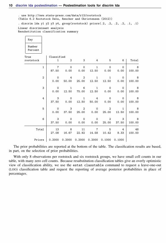
. use http://www.stata-press.com/data/r13/rootstock(Table 6.2 Rootstock Data, Rencher and Christensen (2012))

. discrim lda y1 y2 y3 y4, group(rootstock) priors(.2, .2, .2, .2, .1, .1)

Linear discriminant analysisResubstitution classification summary

Key

NumberPercent

True Classifiedrootstock 1 2 3 4 5 6 Total

1 7 0 0 1 0 0 887.50 0.00 0.00 12.50 0.00 0.00 100.00

2 0 4 2 1 1 0 80.00 50.00 25.00 12.50 12.50 0.00 100.00

3 0 1 6 1 0 0 80.00 12.50 75.00 12.50 0.00 0.00 100.00

4 3 0 1 4 0 0 837.50 0.00 12.50 50.00 0.00 0.00 100.00

5 0 3 2 0 2 1 80.00 37.50 25.00 0.00 25.00 12.50 100.00

6 3 0 0 0 2 3 837.50 0.00 0.00 0.00 25.00 37.50 100.00

Total 13 8 11 7 5 4 4827.08 16.67 22.92 14.58 10.42 8.33 100.00

Priors 0.2000 0.2000 0.2000 0.2000 0.1000 0.1000

The prior probabilities are reported at the bottom of the table. The classification results are based,in part, on the selection of prior probabilities.

With only 8 observations per rootstock and six rootstock groups, we have small cell counts in ourtable, with many zero cell counts. Because resubstitution classification tables give an overly optimisticview of classification ability, we use the estat classtable command to request a leave-one-out(LOO) classification table and request the reporting of average posterior probabilities in place ofpercentages.

discrim lda postestimation — Postestimation tools for discrim lda 11

. estat classtable, probabilities loo

Leave-one-out average-posterior-probabilities classification table

Key

NumberAverage posterior probability

True LOO Classifiedrootstock 1 2 3 4 5 6

1 5 0 0 2 0 10.6055 . . 0.6251 . 0.3857

2 0 4 2 1 1 0. 0.6095 0.7638 0.3509 0.6607 .

3 0 1 6 1 0 0. 0.5520 0.7695 0.4241 . .

4 4 0 1 3 0 00.5032 . 0.7821 0.5461 . .

5 0 3 2 0 2 1. 0.7723 0.5606 . 0.4897 0.6799

6 3 0 0 0 2 30.6725 . . . 0.4296 0.5763

Total 12 8 11 7 5 50.5881 0.6634 0.7316 0.5234 0.4999 0.5589

Priors 0.2000 0.2000 0.2000 0.2000 0.1000 0.1000

Zero cell counts report a missing value for the average posterior probability. We did not specifythe priors() option with estat classtable, so the prior probabilities used in our LDA modelwere used.

estat errorrate estimates the error rates for each group. We use the pp option to obtainestimates based on the posterior probabilities instead of the counts.

. estat errorrate, pp

Error rate estimated from posterior probabilities

rootstockError Rate 1 2 3 4 5

Stratified .2022195 .431596 .0868444 .4899799 .627472

Unstratified .2404022 .41446 .1889412 .5749832 .4953118

Priors .2 .2 .2 .2 .1

rootstockError Rate 6 Total

Stratified .6416429 .3690394

Unstratified .4027382 .3735623

Priors .1

12 discrim lda postestimation — Postestimation tools for discrim lda

We did not specify the priors() option, and estat errorrate defaulted to using the priorprobabilities from the LDA model. Both stratified and unstratified estimates are shown for eachrootstock group and for the overall total. See [MV] discrim estat for an explanation of the error-rateestimation.

We can list the classification results and posterior probabilities from our discriminant analysismodel by using the estat list command. estat list allows us to specify which observations wewish to examine and what classification and probability results to report.

We request the LOO classification and LOO probabilities for all misclassified observations from thefourth rootstock group. We also suppress the resubstitution classification and probabilities from beingdisplayed.

. estat list if rootstock==4, misclassified class(loo noclass) pr(loo nopr)

Classification LOO Probabilities

Obs. True LOO Cl. 1 2 3 4 5 6

25 4 1 * 0.5433 0.1279 0.0997 0.0258 0.0636 0.139726 4 3 * 0.0216 0.0199 0.7821 0.1458 0.0259 0.004827 4 1 * 0.3506 0.1860 0.0583 0.2342 0.0702 0.100829 4 1 * 0.6134 0.0001 0.0005 0.2655 0.0002 0.120232 4 1 * 0.5054 0.0011 0.0017 0.4856 0.0002 0.0059

* indicates misclassified observations

Four of the five misclassifications for rootstock group 4 were incorrectly classified as belongingto rootstock group 1.

ANOVA, MANOVA, and canonical correlations

There is a mathematical relationship between Fisher’s LDA and one-way MANOVA. They are bothbased on the eigenvalues and eigenvectors of the same matrix, W−1B (though in MANOVA thematrices are labeled E and H for error and hypothesis instead of W and B for within and between).See [MV] manova and [R] anova for more information on MANOVA and ANOVA. Researchers oftenwish to examine the MANOVA and univariate ANOVA results corresponding to their LDA model.

Canonical correlations are also mathematically related to Fisher’s LDA. The canonical correlationsbetween the discriminating variables and indicator variables constructed from the group variable arebased on the same eigenvalues and eigenvectors as MANOVA and Fisher’s LDA. The information froma canonical correlation analysis gives insight into the importance of each discriminant function in thediscrimination. See [MV] canon for more information on canonical correlations.

The estat manova, estat anova, and estat canontest commands display MANOVA, ANOVA,and canonical correlation information after discrim lda.

Example 2: MANOVA, ANOVA, and canonical correlation corresponding to LDA

Continuing with the apple tree rootstock example, we examine the MANOVA, ANOVA, and canonicalcorrelation results corresponding to our LDA.

discrim lda postestimation — Postestimation tools for discrim lda 13

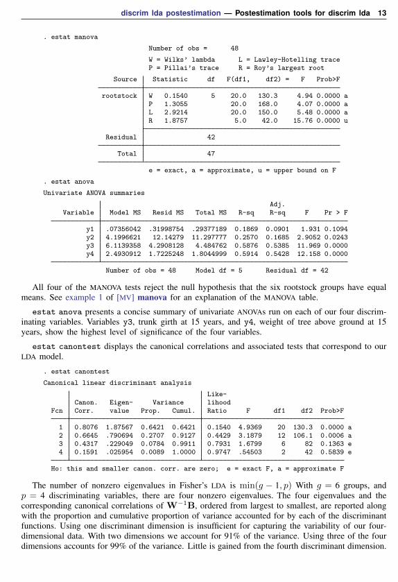
. estat manova

Number of obs = 48

W = Wilks’ lambda L = Lawley-Hotelling traceP = Pillai’s trace R = Roy’s largest root

Source Statistic df F(df1, df2) = F Prob>F

rootstock W 0.1540 5 20.0 130.3 4.94 0.0000 aP 1.3055 20.0 168.0 4.07 0.0000 aL 2.9214 20.0 150.0 5.48 0.0000 aR 1.8757 5.0 42.0 15.76 0.0000 u

Residual 42

Total 47

e = exact, a = approximate, u = upper bound on F

. estat anova

Univariate ANOVA summaries

Adj.Variable Model MS Resid MS Total MS R-sq R-sq F Pr > F

y1 .07356042 .31998754 .29377189 0.1869 0.0901 1.931 0.1094y2 4.1996621 12.14279 11.297777 0.2570 0.1685 2.9052 0.0243y3 6.1139358 4.2908128 4.484762 0.5876 0.5385 11.969 0.0000y4 2.4930912 1.7225248 1.8044999 0.5914 0.5428 12.158 0.0000

Number of obs = 48 Model df = 5 Residual df = 42

All four of the MANOVA tests reject the null hypothesis that the six rootstock groups have equalmeans. See example 1 of [MV] manova for an explanation of the MANOVA table.

estat anova presents a concise summary of univariate ANOVAs run on each of our four discrim-inating variables. Variables y3, trunk girth at 15 years, and y4, weight of tree above ground at 15years, show the highest level of significance of the four variables.

estat canontest displays the canonical correlations and associated tests that correspond to ourLDA model.

. estat canontest

Canonical linear discriminant analysis

Like-Canon. Eigen- Variance lihood

Fcn Corr. value Prop. Cumul. Ratio F df1 df2 Prob>F

1 0.8076 1.87567 0.6421 0.6421 0.1540 4.9369 20 130.3 0.0000 a2 0.6645 .790694 0.2707 0.9127 0.4429 3.1879 12 106.1 0.0006 a3 0.4317 .229049 0.0784 0.9911 0.7931 1.6799 6 82 0.1363 e4 0.1591 .025954 0.0089 1.0000 0.9747 .54503 2 42 0.5839 e

Ho: this and smaller canon. corr. are zero; e = exact F, a = approximate F

The number of nonzero eigenvalues in Fisher’s LDA is min(g − 1, p) With g = 6 groups, andp = 4 discriminating variables, there are four nonzero eigenvalues. The four eigenvalues and thecorresponding canonical correlations of W−1B, ordered from largest to smallest, are reported alongwith the proportion and cumulative proportion of variance accounted for by each of the discriminantfunctions. Using one discriminant dimension is insufficient for capturing the variability of our four-dimensional data. With two dimensions we account for 91% of the variance. Using three of the fourdimensions accounts for 99% of the variance. Little is gained from the fourth discriminant dimension.

14 discrim lda postestimation — Postestimation tools for discrim lda

Also presented are the likelihood-ratio tests of the null hypothesis that each canonical correlationand all smaller canonical correlations from this model are zero. The letter a is placed beside thep-values of the approximate F tests, and the letter e is placed beside the p-values of the exact Ftests. The first two tests are highly significant, indicating that the first two canonical correlations arelikely not zero. The third test has a p-value of 0.1363, so that we fail to reject that the third andfourth canonical correlation are zero.

Discriminant and classification functionsSee [MV] discrim lda for a discussion of linear discriminant functions and linear classification

functions for LDA.

Discriminant functions are produced from Fisher’s LDA. The discriminant functions provide a setof transformations from the original p-dimensional (the number of discriminating variables) space tothe minimum of p and g − 1 (the number of groups minus 1) dimensional space. The discriminantfunctions are ordered in importance.

Classification functions are by-products of the Mahalanobis approach to LDA. There are always gclassification functions—one for each group. They are not ordered by importance, and you cannotuse a subset of them for classification.

A table showing the discriminant function coefficients is available with estat loadings (seeexample 3), and a table showing the classification function coefficients is available with estatclassfunctions (see example 4).

Example 3: Canonical discriminant functions and canonical structures

We continue with the apple tree rootstock example. The canonical discriminant function coefficients(loadings) are available through the estat loadings command. Unstandardized, pooled within-groupstandardized, and total-sample standardized coefficients are available. The all option requests allthree, and the format() option provides control over the numeric display format used in the tables.

. estat loadings, all format(%6.2f)

Canonical discriminant function coefficients

func~1 func~2 func~3 func~4

y1 -3.05 -1.14 -1.00 23.42y2 1.70 -1.22 1.67 -3.08y3 -4.23 7.17 3.05 -2.01y4 0.48 -11.52 -5.51 3.10

_cons 15.45 -12.20 -9.99 -12.47

Standardized canonical discriminant function coefficients

func~1 func~2 func~3 func~4

y1 -0.27 -0.10 -0.09 2.04y2 0.92 -0.65 0.90 -1.65y3 -1.35 2.29 0.97 -0.64y4 0.10 -2.33 -1.12 0.63

Total-sample standardized canonical discriminant function coefficients

func~1 func~2 func~3 func~4

y1 -0.28 -0.10 -0.09 2.14y2 1.00 -0.72 0.99 -1.81y3 -1.99 3.37 1.43 -0.95y4 0.14 -3.45 -1.65 0.93

discrim lda postestimation — Postestimation tools for discrim lda 15

The unstandardized canonical discriminant function coefficients shown in the first table are thefunction coefficients that apply to the unstandardized discriminating variables—y1 through y4 anda constant term. See example 5 for a graph, known as a score plot, that plots the observationstransformed by these unstandardized canonical discriminant function coefficients.

The standardized canonical discriminant function coefficients are the coefficients that apply to thediscriminating variables after they have been standardized by the pooled within-group covariance.These coefficients are appropriate for interpreting the importance and relationship of the discriminatingvariables within the discriminant functions. See example 5 for a graph, known as a loading plot, thatplots these standardized coefficients.

The total-sample standardized canonical discriminant function coefficients are the coefficients thatapply to the discriminating variables after they have been standardized by the total-sample covariance.See Methods and formulas of [MV] discrim lda for references discussing which of within-group andtotal-sample standardization is most appropriate.

For both styles of standardization, variable y1 has small (in absolute value) coefficients for thefirst three discriminant functions. This indicates that y1 does not play an important part in thesediscriminant functions. Because the fourth discriminant function accounts for such a small percentageof the variance, we ignore the coefficients from the fourth function when assessing the importance ofthe variables.

Some sources, see Huberty (1994), advocate the interpretation of structure coefficients, whichmeasure the correlation between the discriminating variables and the discriminant functions, insteadof standardized discriminant function coefficients; see the discussion in example 1 of [MV] discrimlda for references to this dispute. The estat structure command displays structure coefficients.

. estat structure, format(%9.6f)

Canonical structure

function1 function2 function3 function4

y1 -0.089595 -0.261416 0.820783 0.499949y2 -0.086765 -0.431180 0.898063 0.006158y3 -0.836986 -0.281362 0.457902 -0.103031y4 -0.793621 -0.572890 0.162901 -0.124206

Using structure coefficients for interpretation, we conclude that y1 is important for the second andthird discriminant functions.

Example 4: LDA classification functions

Switching from Fisher’s approach to LDA to Mahalanobis’s approach to LDA, we examine what arecalled classification functions with the estat classfunctions command. Classification functionsare applied to the unstandardized discriminating variables. The classification function that results inthe largest value for an observation indicates the group to assign the observation.

Continuing with the rootstock LDA, we specify the format() option to control the display formatof the classification coefficients.

16 discrim lda postestimation — Postestimation tools for discrim lda

. estat classfunctions, format(%8.3f)

Classification functions

rootstock1 2 3 4 5 6

y1 314.640 317.120 324.589 307.260 316.767 311.301y2 -59.417 -63.981 -65.152 -59.373 -65.826 -63.060y3 149.610 168.161 154.910 147.652 168.221 160.622y4 -161.178 -172.644 -150.356 -153.387 -172.851 -175.477

_cons -301.590 -354.769 -330.103 -293.427 -349.847 -318.099

Priors 0.200 0.200 0.200 0.200 0.100 0.100

The prior probabilities, used in constructing the coefficient for the constant term, are displayed asthe last row in the table. We did not specify the priors() option, so the prior probabilities defaultedto those in our LDA model, which has rootstock group 5 and 6 with prior probabilities of 0.1, whereasthe other groups have prior probabilities of 0.2.

See example 10 for applying the classification function to data by using the predict command.

Scree, loading, and score plots

Examples of discriminant function loading plots and score plots (see [MV] scoreplot) can be foundin example 3 of [MV] discrim lda and example 1 of [MV] candisc. Also available after discrimlda are scree plots; see [MV] screeplot.

Example 5: Scree, loading, and score plots

Continuing with our rootstock example, the scree plot of the four nonzero eigenvalues we previouslysaw in the output of estat canontest in example 2 are graphed using the screeplot command.

. screeplot

0.5

11

.52

Eig

en

va

lue

s

1 2 3 4Number

Scree plot of eigenvalues after discrim

discrim lda postestimation — Postestimation tools for discrim lda 17

The Remarks and examples in [MV] screeplot concerning the use of scree plots for selecting thenumber of components in the context of pca apply also for selecting the number of discriminantfunctions after discrim lda. With these four eigenvalues, it is not obvious whether to choose the toptwo or three eigenvalues. From the estat canontest output of example 2, the first two discriminantfunctions account for 91% of the variance, and three discriminant functions account for 99% of thevariance.

The loadingplot command (see [MV] scoreplot) allows us to graph the pooled within-groupstandardized discriminant coefficients (loadings) that we saw in tabular form from the estat loadingscommand of example 3. By default only the loadings from the first two functions are graphed. Weoverride this setting with the components(3) option, obtaining graphs of the first versus second,first versus third, and second versus third function loadings. The combined option switches from amatrix graph to a combined graph. The msymbol(i) option removes the plotting points, leaving thediscriminating variable names in the graph, and the option mlabpos(0) places the discriminatingvariable names in the positions of the plotted points.

. loadingplot, components(3) combined msymbol(i) mlabpos(0)

y1

y2

y3

y4

−2

−1

01

2S

tan

da

rdiz

ed

dis

crim

ina

nt

fun

ctio

n 2

−1.5 −1 −.5 0 .5 1Standardized discriminant function 1

y1

y2y3

y4−1

−.5

0.5

1S

tan

da

rdiz

ed

dis

crim

ina

nt

fun

ctio

n 3

−1.5 −1 −.5 0 .5 1Standardized discriminant function 1

y1

y2y3

y4−1

−.5

0.5

1S

tan

da

rdiz

ed

dis

crim

ina

nt

fun

ctio

n 3

−2 −1 0 1 2Standardized discriminant function 2

Standardized discriminant function loadings

Variable y1, trunk girth at 4 years, is near the origin in all three graphs, indicating that it doesnot play a strong role in discriminating among our six rootstock groups. y4, weight of tree aboveground at 15 years, does not play much of a role in the first discriminant function but does in thesecond and third discriminant functions.

The corresponding three score plots are easily produced with the scoreplot command; see[MV] scoreplot. Score plots graph the discriminant function–transformed observations (called scores).

18 discrim lda postestimation — Postestimation tools for discrim lda

. scoreplot, components(3) combined msymbol(i)

111

1

1

1

1

1

2

2

2

2

2

2

2

2

33

3

3

3

3

3

3

4

4

4

4 4

44 4

5

5

5 5 55

5 5

6

66

6

6

666

−4

−2

02

4

dis

crim

ina

nt

sco

re 2

−4 −2 0 2 4

discriminant score 1

1

11

1

1

11

1

2

22

2

2

2

2

2

3

3

3

3

3

3 334

4

4

44

4

4

4

5

5

5

5 5

5

5

5 6

6

66

66

6

6

−3

−2

−1

01

2

dis

crim

ina

nt

sco

re 3

−4 −2 0 2 4

discriminant score 1

1

1 1

1

1

11

1

2

22

2

2

2

2

2

3

3

3

3

3

33 3 4

4

4

44

4

4

4

5

5

5

55

5

5

5 6

6

66

66

6

6

−3

−2

−1

01

2

dis

crim

ina

nt

sco

re 3

−4 −2 0 2 4

discriminant score 2

Discriminant function scores

There is a lot of overlap, but some separation of the rootstock groups is apparent. One of theobservations from group 6 seems to be sitting by itself in the bottom of the two graphs that havediscriminant function 3 as the y axis. In example 11, we identify this point by using the predictcommand.

Means and distancesThe estat grsummarize command is available after all discrim commands and will display

means, medians, minimums, maximums, standard deviations, group sizes, and more for the groups;see [MV] discrim estat. After discrim lda, the estat grmeans command will also display groupmeans. It, however, has options for displaying the within-group standardized group means, the total-sample standardized group means, and the canonical discriminant functions evaluated at the groupmeans.

Example 6: Standardized group means and canonical discriminant functions at themeans

We introduce the estat grmeans command with the iris data originally from Anderson (1935),introduced in example 3 of [MV] discrim lda.

. use http://www.stata-press.com/data/r13/iris(Iris data)

. discrim lda seplen sepwid petlen petwid, group(iris) notable

The notable option of discrim suppressed the classification table.

By default, estat grmeans displays a table of the means of the discriminating variables for eachgroup. You could obtain the same information along with other statistics with the estat grsummarizecommand; see [MV] discrim estat.

discrim lda postestimation — Postestimation tools for discrim lda 19

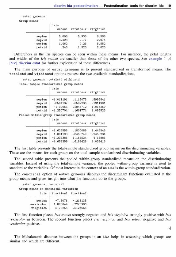
. estat grmeans

Group means

irissetosa versico~r virginica

seplen 5.006 5.936 6.588sepwid 3.428 2.77 2.974petlen 1.462 4.26 5.552petwid .246 1.326 2.026

Differences in the iris species can be seen within these means. For instance, the petal lengthsand widths of the Iris setosa are smaller than those of the other two species. See example 1 of[MV] discrim estat for further exploration of these differences.

The main purpose of estat grmeans is to present standardized or transformed means. Thetotalstd and withinstd options request the two available standardizations.

. estat grmeans, totalstd withinstd

Total-sample standardized group means

irissetosa versico~r virginica

seplen -1.011191 .1119073 .8992841sepwid .8504137 -.6592236 -.1911901petlen -1.30063 .2843712 1.016259petwid -1.250704 .1661774 1.084526

Pooled within-group standardized group means

irissetosa versico~r virginica

seplen -1.626555 .1800089 1.446546sepwid 1.091198 -.8458749 -.2453234petlen -5.335385 1.166534 4.16885petwid -4.658359 .6189428 4.039416

The first table presents the total-sample standardized group means on the discriminating variables.These are the means for each group on the total-sample standardized discriminating variables.

The second table presents the pooled within-group standardized means on the discriminatingvariables. Instead of using the total-sample variance, the pooled within-group variance is used tostandardize the variables. Of most interest in the context of an LDA is the within-group standardization.

The canonical option of estat grmeans displays the discriminant functions evaluated at thegroup means and gives insight into what the functions do to the groups.

. estat grmeans, canonical

Group means on canonical variables

iris function1 function2

setosa -7.6076 -.215133versicolor 1.825049 .7278996virginica 5.78255 -.5127666

The first function places Iris setosa strongly negative and Iris virginica strongly positive with Irisversicolor in between. The second function places Iris virginica and Iris setosa negative and Irisversicolor positive.

The Mahalanobis distance between the groups in an LDA helps in assessing which groups aresimilar and which are different.

20 discrim lda postestimation — Postestimation tools for discrim lda

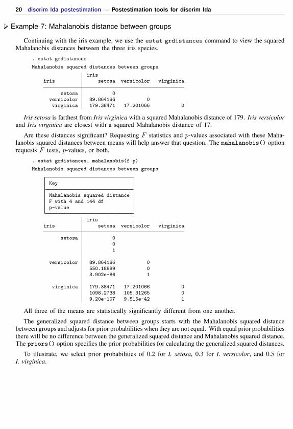
Example 7: Mahalanobis distance between groups

Continuing with the iris example, we use the estat grdistances command to view the squaredMahalanobis distances between the three iris species.

. estat grdistances

Mahalanobis squared distances between groups

irisiris setosa versicolor virginica

setosa 0versicolor 89.864186 0virginica 179.38471 17.201066 0

Iris setosa is farthest from Iris virginica with a squared Mahalanobis distance of 179. Iris versicolorand Iris virginica are closest with a squared Mahalanobis distance of 17.

Are these distances significant? Requesting F statistics and p-values associated with these Maha-lanobis squared distances between means will help answer that question. The mahalanobis() optionrequests F tests, p-values, or both.

. estat grdistances, mahalanobis(f p)

Mahalanobis squared distances between groups

Key

Mahalanobis squared distanceF with 4 and 144 dfp-value

irisiris setosa versicolor virginica

setosa 001

versicolor 89.864186 0550.18889 03.902e-86 1

virginica 179.38471 17.201066 01098.2738 105.31265 09.20e-107 9.515e-42 1

All three of the means are statistically significantly different from one another.

The generalized squared distance between groups starts with the Mahalanobis squared distancebetween groups and adjusts for prior probabilities when they are not equal. With equal prior probabilitiesthere will be no difference between the generalized squared distance and Mahalanobis squared distance.The priors() option specifies the prior probabilities for calculating the generalized squared distances.

To illustrate, we select prior probabilities of 0.2 for I. setosa, 0.3 for I. versicolor, and 0.5 forI. virginica.

discrim lda postestimation — Postestimation tools for discrim lda 21

. estat grdistances, generalized priors(.2, .3, .5)

Generalized squared distances between groups

irisiris setosa versicolor virginica

setosa 3.2188758 92.272131 180.77101versicolor 93.083061 2.4079456 18.587361virginica 182.60359 19.609012 1.3862944

This matrix is not symmetric and does not have zeros on the diagonal.

Covariance and correlation matricesEqual group covariance matrices is an important assumption underlying LDA. The estat

covariance command displays the group covariance matrices, the pooled within-group covari-ance matrix, the between-groups covariance matrix, and the total-sample covariance matrix. Theestat correlation command provides the corresponding correlation matrices, with an option topresent p-values with the correlations.

Example 8: Group covariances and correlations

Continuing our examination of LDA on the iris data, we request to see the pooled within-groupcovariance matrix and the covariance matrices for the three iris species.

. estat covariance, within groups

Pooled within-group covariance matrix

seplen sepwid petlen petwid

seplen .2650082sepwid .0927211 .1153878petlen .1675143 .0552435 .1851878petwid .0384014 .0327102 .0426653 .0418816

Group covariance matrices

iris: setosa

seplen sepwid petlen petwid

seplen .124249sepwid .0992163 .1436898petlen .0163551 .011698 .0301592petwid .0103306 .009298 .0060694 .0111061

iris: versicolor

seplen sepwid petlen petwid

seplen .2664327sepwid .0851837 .0984694petlen .182898 .0826531 .2208163petwid .0557796 .0412041 .073102 .0391061

iris: virginica

seplen sepwid petlen petwid

seplen .4043429sepwid .0937633 .1040041petlen .3032898 .0713796 .3045878petwid .0490939 .0476286 .0488245 .0754327

22 discrim lda postestimation — Postestimation tools for discrim lda

All variables have positive covariance—not surprising for physical measurements (length andwidth).

We could have requested the between-groups covariance matrix and the total-sample covariancematrix. Options of estat covariance control how the covariance matrices are displayed.

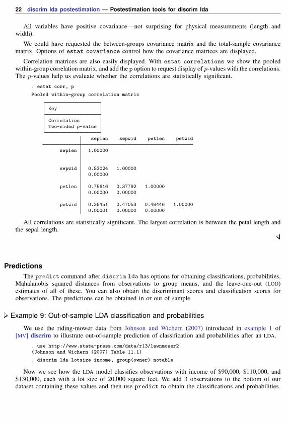
Correlation matrices are also easily displayed. With estat correlations we show the pooledwithin-group correlation matrix, and add the p option to request display of p-values with the correlations.The p-values help us evaluate whether the correlations are statistically significant.

. estat corr, p

Pooled within-group correlation matrix

Key

CorrelationTwo-sided p-value

seplen sepwid petlen petwid

seplen 1.00000

sepwid 0.53024 1.000000.00000

petlen 0.75616 0.37792 1.000000.00000 0.00000

petwid 0.36451 0.47053 0.48446 1.000000.00001 0.00000 0.00000

All correlations are statistically significant. The largest correlation is between the petal length andthe sepal length.

PredictionsThe predict command after discrim lda has options for obtaining classifications, probabilities,

Mahalanobis squared distances from observations to group means, and the leave-one-out (LOO)estimates of all of these. You can also obtain the discriminant scores and classification scores forobservations. The predictions can be obtained in or out of sample.

Example 9: Out-of-sample LDA classification and probabilities

We use the riding-mower data from Johnson and Wichern (2007) introduced in example 1 of[MV] discrim to illustrate out-of-sample prediction of classification and probabilities after an LDA.

. use http://www.stata-press.com/data/r13/lawnmower2(Johnson and Wichern (2007) Table 11.1)

. discrim lda lotsize income, group(owner) notable

Now we see how the LDA model classifies observations with income of $90,000, $110,000, and$130,000, each with a lot size of 20,000 square feet. We add 3 observations to the bottom of ourdataset containing these values and then use predict to obtain the classifications and probabilities.

discrim lda postestimation — Postestimation tools for discrim lda 23

. input

owner income lots~e25. . 90 2026. . 110 2027. . 130 2028. end

. predict grp in 25/L, class(24 missing values generated)

. predict pr* in 25/L, pr(24 missing values generated)

. list in 25/L

owner income lotsize grp pr1 pr2

25. . 90.0 20.0 0 .5053121 .494687926. . 110.0 20.0 1 .1209615 .879038527. . 130.0 20.0 1 .0182001 .9818

The observation with income of $90,000 was classified as a nonowner, but it was a close decisionwith probabilities of 0.505 for nonowner and 0.495 for owner. The two other observations, with$110,000 and $130,000 income, were classified as owners, with higher probability of ownership forthe higher income.

The estat list, estat classtable, and estat errorrate commands (see [MV] discrimestat) obtain their information by calling predict. The LOO listings and tables from these commandsare obtained by calling predict with the looclass and loopr options.

In addition to predictions and probabilities, we can obtain the classification scores for observations.

Example 10: Classification scores

In example 4, we used the estat classfunctions command to view the classification functionsfor the LDA of the apple tree rootstock data. We can use predict to obtain the correspondingclassification scores—the classification function applied to observations.

. use http://www.stata-press.com/data/r13/rootstock, clear(Table 6.2 Rootstock Data, Rencher and Christensen (2012))

. discrim lda y1 y2 y3 y4, group(rootstock) priors(.2,.2,.2,.2,.1,.1) notable

. predict clscr*, clscore

. format clscr* %6.1f

. list rootstock clscr* in 1/3, noobs

rootst~k clscr1 clscr2 clscr3 clscr4 clscr5 clscr6

1 308.1 303.7 303.1 307.1 303.5 307.11 327.6 324.1 322.9 326.1 323.3 326.01 309.5 308.2 306.3 309.3 307.5 309.0

24 discrim lda postestimation — Postestimation tools for discrim lda

We did not specify the priors() option, so predict used the prior probabilities that werespecified with our LDA model in determining the constant term in the classification function; seeexample 4 for a table of the classification functions. Observations may be classified to the group withlargest score. The first 3 observations belong to rootstock group 1 and are successfully classified asbelonging to group 1 because the classification score in clscr1 is larger than the classification scoresfor the other groups.

Scoring the discriminating variables by using Fisher’s canonical discriminant functions is accom-plished with the dscore option of predict.

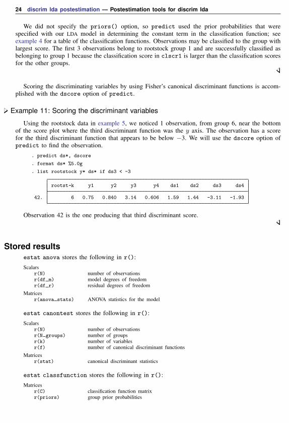
Example 11: Scoring the discriminant variables

Using the rootstock data in example 5, we noticed 1 observation, from group 6, near the bottomof the score plot where the third discriminant function was the y axis. The observation has a scorefor the third discriminant function that appears to be below −3. We will use the dscore option ofpredict to find the observation.

. predict ds*, dscore

. format ds* %5.0g

. list rootstock y* ds* if ds3 < -3

rootst~k y1 y2 y3 y4 ds1 ds2 ds3 ds4

42. 6 0.75 0.840 3.14 0.606 1.59 1.44 -3.11 -1.93

Observation 42 is the one producing that third discriminant score.

Stored resultsestat anova stores the following in r():

Scalarsr(N) number of observationsr(df m) model degrees of freedomr(df r) residual degrees of freedom

Matricesr(anova stats) ANOVA statistics for the model

estat canontest stores the following in r():

Scalarsr(N) number of observationsr(N groups) number of groupsr(k) number of variablesr(f) number of canonical discriminant functions

Matricesr(stat) canonical discriminant statistics

estat classfunction stores the following in r():

Matricesr(C) classification function matrixr(priors) group prior probabilities

discrim lda postestimation — Postestimation tools for discrim lda 25

estat correlations stores the following in r():

Matricesr(Rho) pooled within-group correlation matrix (within only)r(P) two-sided p-values for pooled within-group correlations (within and p only)r(Rho between) between-groups correlation matrix (between only)r(P between) two-sided p-values for between-groups correlations (between and p only)r(Rho total) total-sample correlation matrix (total only)r(P total) two-sided p-values for total-sample correlations (total and p only)r(Rho #) group # correlation matrix (groups only)r(P #) two-sided p-values for group # correlations (groups and p only)

estat covariance stores the following in r():

Matricesr(S) pooled within-group covariance matrix (within only)r(S between) between-groups covariance matrix (between only)r(S total) total-sample covariance matrix (total only)r(S #) group # covariance matrix (groups only)

estat grdistances stores the following in r():

Scalarsr(df1) numerator degrees of freedom (mahalanobis only)r(df2) denominator degrees of freedom (mahalanobis only)

Matricesr(sqdist) Mahalanobis squared distances between group means (mahalanobis only)r(F sqdist) F statistics for tests that the Mahalanobis squared distances between group means

are zero (mahalanobis only)r(P sqdist) p-value for tests that the Mahalanobis squared distances between group means are

zero (mahalanobis only)r(gsqdist) generalized squared distances between group means (generalized only)

estat grmeans stores the following in r():

Matricesr(means) group means (raw only)r(stdmeans) total-sample standardized group means (totalstd only)r(wstdmeans) pooled within-group standardized group means (withinstd only)r(cmeans) group means on canonical variables (canonical only)

estat loadings stores the following in r():

Matricesr(L std) Within-group standardized canonical discriminant function coefficients

(standardized only)r(L totalstd) total-sample standardized canonical discriminant function coefficients

(totalstandardized only)r(L unstd) unstandardized canonical discriminant function coefficients

(unstandardized only)

estat manova stores the following in r():

Scalarsr(N) number of observationsr(df m) model degrees of freedomr(df r) residual degrees of freedom

Matricesr(stat m) multivariate statistics for the model

26 discrim lda postestimation — Postestimation tools for discrim lda

estat structure stores the following in r():

Matricesr(canstruct) canonical structure matrix

Methods and formulasSee Methods and formulas of [MV] discrim lda for background on what is produced by predict,

estat classfunctions, estat grdistances, estat grmeans, estat loadings, and estatstructure. See [MV] discrim estat for more information on estat classtable, estat errorrate,estat grsummarize, and estat list. See [R] anova for background information on the ANOVAssummarized by estat anova; see [MV] manova for information on the MANOVA shown by estatmanova; and see [MV] canon for background information on canonical correlations and related testsshown by estat canontest.

ReferencesAnderson, E. 1935. The irises of the Gaspe Peninsula. Bulletin of the American Iris Society 59: 2–5.

Andrews, D. F., and A. M. Herzberg, ed. 1985. Data: A Collection of Problems from Many Fields for the Studentand Research Worker. New York: Springer.

Huberty, C. J. 1994. Applied Discriminant Analysis. New York: Wiley.

Johnson, R. A., and D. W. Wichern. 2007. Applied Multivariate Statistical Analysis. 6th ed. Englewood Cliffs, NJ:Prentice Hall.

Rencher, A. C., and W. F. Christensen. 2012. Methods of Multivariate Analysis. 3rd ed. Hoboken, NJ: Wiley.

Also see[MV] discrim lda — Linear discriminant analysis

[MV] discrim estat — Postestimation tools for discrim

[MV] scoreplot — Score and loading plots

[MV] screeplot — Scree plot

[MV] candisc — Canonical linear discriminant analysis

[MV] canon — Canonical correlations

[MV] discrim — Discriminant analysis

[MV] manova — Multivariate analysis of variance and covariance

[U] 20 Estimation and postestimation commands