Tindall Aquifer Water Trading Model: Technical Report and Scenario Results

Tindall Aquifer Water Trading Model: Technical Report and Scenario Results

Scott Heckbert, Alex Smajgl and Anna Straton

CSIRO Sustainable Ecosystems

September 2006

Tindall Aquifer Water Trading Model: Technical Report and Scenario Results

Scott Heckbert, Alex Smajgl and Anna Straton

CSIRO Sustainable Ecosystems, Townsville and Darwin

September 2006

Enquiries should be addressed to:

Scott Heckbert Davies Laboratory CSIRO Sustainable Ecosystems PMB Aitkenvale 4814 Ph: + 61 7 4753 8593 Fax: +61 7 4753 8600 Email: [email protected]

Important Notice

© CSIRO. This work is subject to copyright. The reproduction in whole or in part for study or training purposes is granted subject to inclusion of an acknowledgment of the source. The Copyright Act 1968 governs any other reproduction of this document.

CSIRO Sustainable Ecosystems advises that the information contained in this publication comprises general statements based on scientific research. The views expressed, except where stated otherwise, and the conclusions reached in this publication are those of the author(s) of the reporting pages, and not necessarily those of CSIRO Sustainable Ecosystems. The reader is advised and needs to be aware that any such scientific information and views may be incomplete or unable to be used in any specific situation. No reliance or actions must therefore be made on that information without seeking prior expert professional, scientific and technical advice. To the extent permitted by law, CSIRO Sustainable Ecosystems (including its employees and consultants) excludes all liability to any person for any consequences, including but not limited to all losses, damages, costs, expenses and any other compensation, arising directly or indirectly form using this publication (in part or in whole) and any information or material contained in it.

This publication is available in an electronic format from: http://www.cse.csiro.au/publications/reports.htm

mailto:[email protected]

Table of Contents 1. Introduction .................................................................................................... 1 2. Model Structure and Interface........................................................................ 3

2.1 Program Architecture.............................................................................. 3 2.2 User Interface and Scenario Specifications ............................................ 4

3. Model Processes ........................................................................................... 5 3.1 Rainfall and Hydrological Conditions ...................................................... 5 3.2 Regulating Groundwater Extraction Levels............................................. 7 3.3 Producer Characteristics and Behaviours............................................... 8 3.4 Water Market Decisions.......................................................................... 9 3.5 Calculating Agents’ Market Price for Water .......................................... 11 3.6 Experimentally-calibrated Bidding Behaviour ....................................... 15 3.7 Market Structure ................................................................................... 22 3.8 Production Outcomes ........................................................................... 23 3.9 Adaptive behaviour ............................................................................... 26

4. Results......................................................................................................... 28 4.1 Scenario 1: Baseline Conditions: No-trade , no new licenses granted . 28 4.2 Scenario 2: Limited applications granted, no trade............................... 30 4.3 Scenario 3: Applications granted, water market implemented, all

growers bear risk of water restrictions .................................................. 33 4.4 Scenario 4: Applications granted, market created, newcomers bear risk

of pumping restrictions.......................................................................... 40 4.5 Scenario 5: Applications granted, market created, trading between east

and west Tindall restricted .................................................................... 47 5. Discussion ................................................................................................... 50 References ......................................................................................................... 52 List of Figures Figure 1: Farms included in the Tindall Aquifer Water Trading Model .............................. 2 Figure 2: The Repast user interface of the Tindall Aquifer Water Trading Model. ............ 4 Figure 3: Repast graphical output of historical rainfall data for the Katherine Region,

1975 to 2005. ............................................................................................................. 6 Figure 4: Bidding Strategy 1: Consistent mark-up value for selling bids......................... 16 Figure 5: Strategy 2: Increasing mark-up value .............................................................. 16 Figure 6: Strategy 3: Increasing mark-up value .............................................................. 17 Figure 7: Strategy 4: Converging mark-up value ............................................................ 17 Figure 8: Strategy 5: Consistent mark-up value, attempting a higher mark up value in

high-use periods ...................................................................................................... 18 Figure 9: Strategy 6: Consistent mark-up value for buying and selling bids ................... 18 Figure 10: Strategy 7: Consistent mark-up value for buying bids ................................... 19

Figure 11: Strategy 8: Converging mark-up value for buying and selling bids................ 19 Figure 12: Strategy 9: Converging and overshooting mark-up value for buying ............ 20 Figure 13: Strategy 10: Converging mark-up value and stochastic shock for buying bids

................................................................................................................................. 20 Figure 14: Strategy 11: Converging mark-up value and stochastic shock for buying and

selling bids ............................................................................................................... 21 Figure 15: Number of agents employing the eleven bidding strategies. ......................... 22 Figure 16: Total groundwater extraction by irrigating growers, showing rainfall and

available extraction volumes, and the associated extraction levels for Scenario 1, showing baseline conditions. ................................................................................... 28

Figure 17: Total profit from irrigated horticulture, Scenario 1, showing baseline conditions and prices for produce (mangoes) ........................................................................... 29

Figure 18: Total profit under the baseline scenario compared to profit levels possible with unrestricted access to labour ................................................................................... 30

Figure 19: Number of growers who seek off-farm income through the modelled adaptation process under the baseline scenario ..................................................... 30

Figure 20: Groundwater volume available for extraction and licensed volumes for three scenarios.................................................................................................................. 31

Figure 21: Total groundwater extraction by irrigating growers, showing mean values and associated confidence intervals, Scenarios 1 and 2b .............................................. 32

Figure 22: Total profit from irrigated horticulture, Scenario 2b, showing mean values and associated confidence intervals. .............................................................................. 33

Figure 23: Total groundwater extraction by irrigating growers, Scenarios 1 and 3, showing mean values and associated confidence intervals. ................................... 34

Figure 24: Total profit from irrigated horticulture, Scenarios 1 and 3, showing mean values and associated confidence intervals............................................................. 35

Figure 25: Percentage by which licenses will be restricted, Scenarios 1 and 3.............. 36 Figure 26: Volume of water demanded and supplied within the water market, Scenario 3

................................................................................................................................. 36 Figure 27: Volume purchased on the water market and average bid per Ml of water,

Scenario 3................................................................................................................ 37 Figure 28: Revenues realised from activity in the water market, Scenario 3. ................. 38 Figure 29: Aggregate production levels, Scenario 3, compared to unlimited water

availability, showing mean values and associated confidence intervals.................. 38 Figure 30: Number of growers who seek off-farm income, Scenarios 1 and 3 ............... 39 Figure 31: Total groundwater extraction by irrigating growers, comparing scenarios 3 and

scenario 4, where newcomers must solely bear the burden of water restrictions, showing mean values and associated confidence intervals. ................................... 41

Figure 32: Profit from irrigated horticulture, Scenarios 3 and 4, showing mean values and associated confidence intervals. .............................................................................. 42

Figure 33: Shannon Diversity Index of profit, Scenarios 3 and 4, showing mean values and associated confidence intervals. ....................................................................... 43

Figure 34 Average profitability by farm size for an typical year, scenario 3 .................... 43

Figure 35: Percentage by which licenses will be restricted, Scenarios 3 and 4.............. 44 Figure 36: Volume of water demanded, comparing scenarios 3 and scenario 4 where

newcomers must solely bear the burden of water restrictions, showing mean values and associated confidence intervals. ....................................................................... 44

Figure 37: Volume of water purchased in the market, Scenarios 3 and 4, showing mean values and associated confidence intervals............................................................. 45

Figure 38: Volume of water supplied to the market, Scenarios 3 and 4, showing mean values and associated confidence intervals............................................................. 45

Figure 39: Average bid per Ml of water, Scenarios 3 and 4, showing mean values and associated confidence intervals. .............................................................................. 46

Figure 40: Total water revenues derived from the water market, Scenarios 3 and 4, showing mean values and associated confidence intervals. ................................... 46

Figure 41: Number of growers who seek off-farm income, Scenarios 3 and 4 ............... 47 Figure 42: Total groundwater extraction by irrigating growers, comparing scenarios 3 and

scenario 5, where trade between the East and West Tindall areas is restricted, showing mean values and associated confidence intervals. ................................... 48

Figure 43: Profit from irrigated horticulture, Scenarios 3 and 5, showing mean values and associated confidence intervals. .............................................................................. 48

Figure 44: Volume of water demanded, Scenarios 3 and 5, showing mean values and associated confidence intervals. .............................................................................. 49

Figure 45: Average bid per Ml of water, Scenarios 3 and 5, showing mean values and associated confidence intervals. .............................................................................. 49

Figure 46: Volume of water purchased from the market, Scenarios 3 and 5, showing mean values and associated confidence intervals................................................... 50

Figure 47: Water revenues derived from activity on the water market, Scenarios 3 and 5, showing mean values and associated confidence intervals. ................................... 50

Acknowledgements The research team wishes to thank Freeman Cook and Kostas Alexandridis for helpful

comments during review. We would also like to thank members of NT Department of

Natural Resources, Environment and the Arts and the Department of Primary Industry,

Fisheries and Mines, especially Ian Smith, Matt Darcey, Debbie Rock, Julie Bird, Claire

Hill, Caroline Green, Chris Wicks, Peter Jolly, Steven Tickell, Ian Lancaster, and Des Yin

Foo.

The members of the research team thank the Tropical Savannas Cooperative Research

Centre (CRC), and the Commonwealth Scientific and Industrial Research Organisation

(CSIRO) Social and Economic Integration Emerging Science Area for providing the

support and project funding to undertake this research. We also include the Desert

Knowledge CRC in this list to thank for funding the umbrella ‘Outback Institutions’ project

of which this case study is a part.

1. Introduction This paper describes the functioning of the Tindall Aquifer Water Trading Model,

developed by CSIRO Sustainable Ecosystems. The model is used for simulating

a hypothetical market for water where irrigators in the Katherine region of the

Northern Territory, Australia, may buy and sell their groundwater entitlements.

The Tindall aquifer discharges into the Katherine River and is largely responsible

for the flow of water occurring in the river throughout the year, and particularly in

the dry season (Puhalovich 2005). The aquifer also provides water for irrigators

for use in agricultural / horticultural production.

The introduction of water trading systems in Australia has been proposed as part

of the National Water Initiative1 as an allocation mechanism that may improve

rural water use efficiency and help manage environmental outcomes as demand

from irrigators increases. Increased groundwater pumping levels could potentially

reduce the volume of water discharged into the river, and in turn affect

environmental services which depend on the river’s water flow.

The Tindall Aquifer Water Trading Model focuses specifically on extraction of

groundwater from the Tindall aquifer for the purposes of horticultural production.

Here we simulate a hypothetical water market for growers in the region, and use

the simulation to examine outcomes that emerge depending on various scenarios

of the market is implemented operated into the future.

Within the model, simulated growers are allocated a monthly licensed volume of

groundwater for use in irrigated production, with model input data based on a

number of real-world data sources from the region. Within the model, water can

be applied to crops or sold to other growers for this purpose. The model

considers water allocated to horticultural/agricultural uses, and does not consider

water allocated to the public water supply, industrial use, or other uses. The

model considers growers living in an area in and around Katherine and extracting

from the Tindall aquifer, as depicted in the darker green area of Figure 1.

The model simulates conditions for a number of possible scenarios. Baseline

conditions include n=18 growers, allocated a total annual volume of 18,990 Ml to 1 See http://www.nwc.gov.au/NWI/index.cfm

1

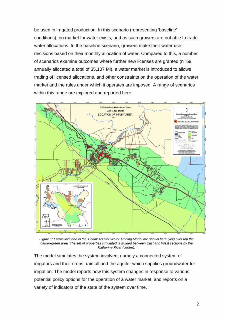
be used in irrigated production. In this scenario (representing ‘baseline’

conditions), no market for water exists, and as such growers are not able to trade

water allocations. In the baseline scenario, growers make their water use

decisions based on their monthly allocation of water. Compared to this, a number

of scenarios examine outcomes where further new licenses are granted (n=59

annually allocated a total of 35,107 Ml), a water market is introduced to allows

trading of licensed allocations, and other constraints on the operation of the water

market and the rules under which it operates are imposed. A range of scenarios

within this range are explored and reported here.

Figure 1: Farms included in the Tindall Aquifer Water Trading Model are shown here lying over top the darker-green area. The set of properties simulated is divided between East and West sections by the

Katherine River (centre).

The model simulates the system involved, namely a connected system of

irrigators and their crops, rainfall and the aquifer which supplies groundwater for

irrigation. The model reports how this system changes in response to various

potential policy options for the operation of a water market, and reports on a

variety of indicators of the state of the system over time.

2

This report describes the model’s operations and results according to a number

of scenarios. Section 2 describes the model structure, including the program

architecture, user interface and scenario specifications. Section 3 describes

details of model operations, describing each program module, including

equations, assumptions and calibration of the model. This section is organised

according to the order of execution of the model. Section 4 describes simulation

results of the water market for a number of scenarios. Section 5 offers discussion

of simulation results.

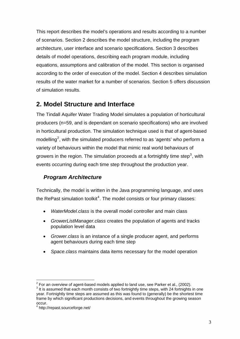
2. Model Structure and Interface The Tindall Aquifer Water Trading Model simulates a population of horticultural

producers (n=59, and is dependant on scenario specifications) who are involved

in horticultural production. The simulation technique used is that of agent-based

modelling2, with the simulated producers referred to as ‘agents’ who perform a

variety of behaviours within the model that mimic real world behaviours of

growers in the region. The simulation proceeds at a fortnightly time step3, with

events occurring during each time step throughout the production year.

Program Architecture

Technically, the model is written in the Java programming language, and uses

the RePast simulation toolkit4. The model consists or four primary classes:

• WaterModel.class is the overall model controller and main class

• GrowerListManager.class creates the population of agents and tracks population level data

• Grower.class is an instance of a single producer agent, and performs agent behaviours during each time step

• Space.class maintains data items necessary for the model operation

2 For an overview of agent-based models applied to land use, see Parker et al., (2002). 3 It is assumed that each month consists of two fortnightly time steps, with 24 fortnights in one year. Fortnightly time steps are assumed as this was found to (generally) be the shortest time frame by which significant productions decisions, and events throughout the growing season occur. 4 http://repast.sourceforge.net/

3

Further classes are included to support this basic structure. Upon initialisation,

the model progresses through the steps outlined in this paper calling methods

(functions) from the above classes where appropriate.

User Interface and Scenario Specifications

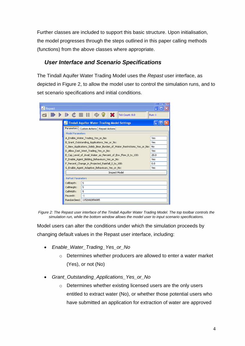
The Tindall Aquifer Water Trading Model uses the Repast user interface, as

depicted in Figure 2, to allow the model user to control the simulation runs, and to

set scenario specifications and initial conditions.

Figure 2: The Repast user interface of the Tindall Aquifer Water Trading Model. The top toolbar controls the

simulation run, while the bottom window allows the model user to input scenario specifications.

Model users can alter the conditions under which the simulation proceeds by

changing default values in the Repast user interface, including:

• Enable_Water_Trading_Yes_or_No

o Determines whether producers are allowed to enter a water market

(Yes), or not (No)

• Grant_Outstanding_Applications_Yes_or_No

o Determines whether existing licensed users are the only users

entitled to extract water (No), or whether those potential users who

have submitted an application for extraction of water are approved

4

to pump ground water (Yes), as based on DNRETA5 water license

data

• New_Applications_Solely_Bear_Burden_of_Water_Restrictions_Yes_or_N

o Sets whether ‘newcomers’ into the community of licensed water

users are the only users affected by the imposition of pumping

restrictions (Yes), or if all water users equally are affected (No)

• Allow_East_West_Trading_Yes_or_No

o Sets whether producers located in the East Tindall area (n=32,

including applicants) may trade with producers located in the West

Tindall area (n=27) (Yes) or whether producers in the East and

West may only trade amongst themselves (No)

• Percent_Change_in_Projected_Rainfall_0_to_100

o Sets the increase or decrease in rainfall as a percentage change of

the historical rainfall patterns

• Cap_Level_of_Avail_Water_as_Percent_of_Env_Flow_0_to_100

o Sets the minimum percentage of natural environmental flows that

must be maintained. The remainder is available for groundwater

extraction.

3. Model Processes Rainfall and Hydrological Conditions

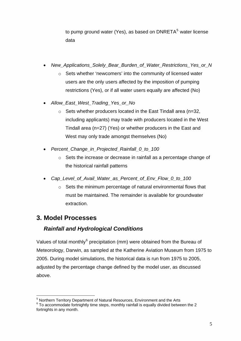
Values of total monthly6 precipitation (mm) were obtained from the Bureau of

Meteorology, Darwin, as sampled at the Katherine Aviation Museum from 1975 to

2005. During model simulations, the historical data is run from 1975 to 2005,

adjusted by the percentage change defined by the model user, as discussed

above.

5 Northern Territory Department of Natural Resources, Environment and the Arts 6 To accommodate fortnightly time steps, monthly rainfall is equally divided between the 2 fortnights in any month.

5

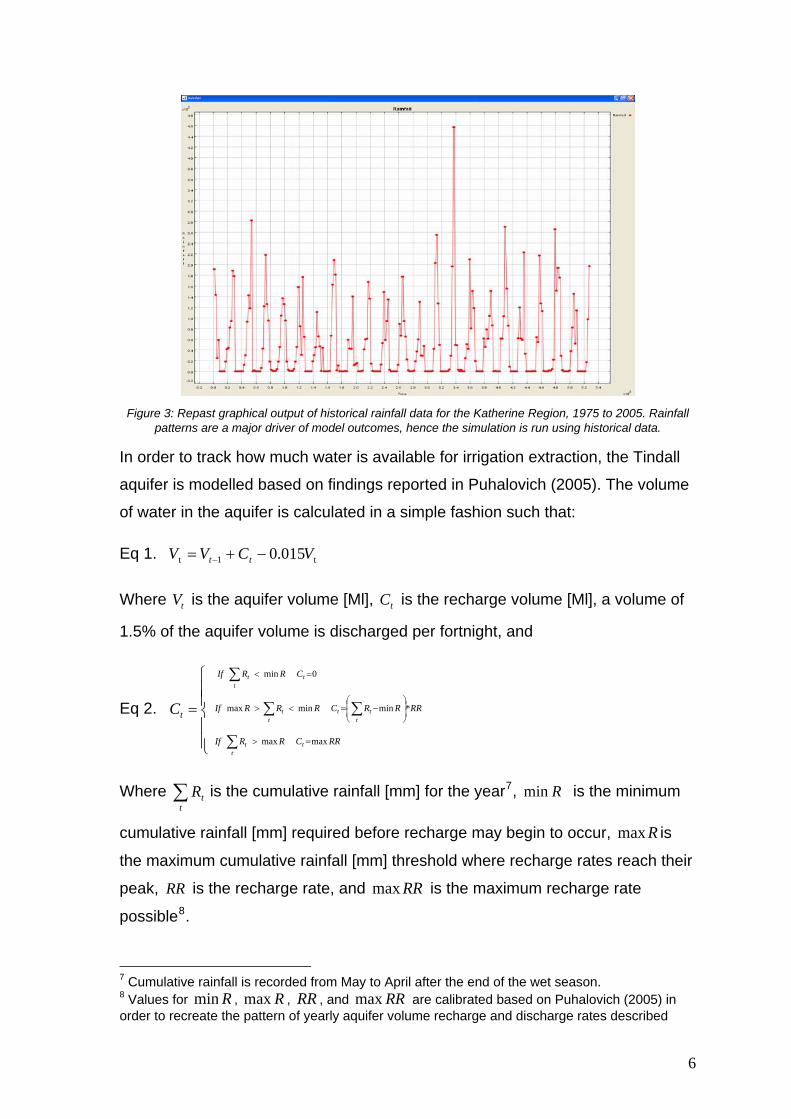
Figure 3: Repast graphical output of historical rainfall data for the Katherine Region, 1975 to 2005. Rainfall

patterns are a major driver of model outcomes, hence the simulation is run using historical data.

In order to track how much water is available for irrigation extraction, the Tindall

aquifer is modelled based on findings reported in Puhalovich (2005). The volume

of water in the aquifer is calculated in a simple fashion such that:

Eq 1. t1t 015.0 VCVV tt −+= −

Where is the aquifer volume [Ml], is the recharge volume [Ml], a volume of

1.5% of the aquifer volume is discharged per fortnight, and

tV tC

Eq 2.

⎪⎪⎩

⎪⎪⎨

⎧

∑

∑∑

∑

=

=>

⎟⎟⎠

⎞⎜⎜⎝

⎛−=<>

=<

ttt

ttt

tt

ttt

RRCRRIf

RRRRCRRRIf

CRRIf

tC

max

max

*min

min

max

0 min

Where is the cumulative rainfall [mm] for the year∑t

tR 7, Rmin is the minimum

cumulative rainfall [mm] required before recharge may begin to occur, is

the maximum cumulative rainfall [mm] threshold where recharge rates reach their

peak,

Rmax

RR is the recharge rate, and is the maximum recharge rate

possible

RRmax8.

7 Cumulative rainfall is recorded from May to April after the end of the wet season. 8 Values for Rmin , , Rmax RR , and are calibrated based on Puhalovich (2005) in order to recreate the pattern of yearly aquifer volume recharge and discharge rates described

RRmax

6

Regulating Groundwater Extraction Levels

A certain level of acceptable environmental flow of water into the Katherine River

is defined by the model user through the user interface, as described in section 4,

above. At least 80% of annual aquifer recharge is to be allocated for

environmental use for the purpose of ensuring that requirements of all

groundwater-dependent ecosystems are maintained. Annual extraction from

aquifers will therefore be equivalent to no more than 20% of annual recharge

(Faulks and Kirby 2004). This is known as the ‘80:20 rule’. This determines the

minimum level of groundwater extraction. Past this point, extraction levels are

‘capped’9, thereby maintaining this minimum acceptable volume and hence the

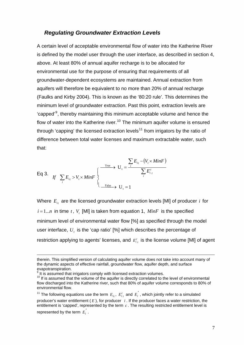
flow of water into the Katherine river.10 The minimum aquifer volume is ensured

through ‘capping’ the licensed extraction levels11 from irrigators by the ratio of

difference between total water licenses and maximum extractable water, such

that:

Eq 3.

( )

1 U

U

tFalse

tTrue

=⎯⎯→⎯⎪⎩

⎪⎨⎧

×−=⎯⎯→⎯

×>∑

∑

∑ it

ci

ti

ti

ti

ti

E

MinFVE

MinFVEIf

Where are the licensed groundwater extraction levels [Ml] of producer i for

in time , [Ml] is taken from equation 1, is the specified

minimum level of environmental water flow [%] as specified through the model

user interface, is the ‘cap ratio’ [%] which describes the percentage of

restriction applying to agents’ licenses, and is the license volume [Ml] of agent

tiE

ni ...1= t tV MinF

tU

tiEc

therein. This simplified version of calculating aquifer volume does not take into account many of the dynamic aspects of effective rainfall, groundwater flow, aquifer depth, and surface evapotranspiration. 9 It is assumed that irrigators comply with licensed extraction volumes. 10 If is assumed that the volume of the aquifer is directly correlated to the level of environmental flow discharged into the Katherine river, such that 80% of aquifer volume corresponds to 80% of environmental flow. 11 The following equations use the term , and tiE t

ciE ′

iE , which jointly refer to a simulated producer’s water entitlement ( E ), for producer . If the producer faces a water restriction, the entitlement is ‘capped’, represented by the term c . The resulting restricted entitlement level is represented by the term .

i

′iE

7

i to which the cap c applies, again as specified by the model user. For example,

if the model user has defined that only ‘newcomers’ are to bear the burden of

water restrictions, represents the total license volume of only this portion of

the agent population. Where no conditions of distribution for the burden of water

restrictions exist, the burden is borne equally

∑i

tiEc

12 for all agents in the population of

irrigators. This process alters the licensed amount of groundwater an agent may

extract, such that:

Eq 4. ⎪⎩

⎪⎨⎧

=

==′

1 *

0

cifUE

cifEE

ti

i

ti

t

t

Where is the adjusted licensed volume [Ml], and c is a binary variable (1 or 0)

which is ‘on’ if restrictions apply to that agent, otherwise is ‘off’.

′iE

The outcome of equations 2 and 3 is a specified volume of water that is restricted

from being extracted by irrigators, and the determination of how that capped

volume is distributed across the agent population (i.e. whether restrictions are

borne equally or only by a certain group of irrigators).

Producer Characteristics and Behaviours

Data for farm attributes was acquired from DNRETA for calibration of simulated

agents13. From this, the data set (held within the file ‘ProducerData.csv’) informs

the model of attributes for each groundwater pumping license, including the

details of each agent’s water entitlements and other information pertinent to the

farm’s operation, including:

• Area14

• Location on either the east or west portion of the aquifer

• Whether the license is currently allocated or is in the application stage

12 Licenses are adjusted by a percentage of the original license volume, where the percentage of the license is equal for all affected producers. I.e. all licenses could hypothetically be capped by 10% of their original volume, and hence larger licensed volumes would account for larger actually volume of water restricted from pumping. 13 The data set was truncated to include only those licenses involved in irrigation activities, and excludes water use for industrial, cultural and public water use purposes. 14 The spatial extend of the area under analysis is 33622.09 ha based on DNRETA data

8

• Current licensed extraction amounts (Ml) for months January through

December15

• Area of land under production

Although a number of land uses exist in the study regions,16 model operations

are calibrated to mango production data. This assumption was required due to

lack of consistent data.

Water Market Decisions

At this stage of the model process, the conditions for rainfall, aquifer condition,

agents’ water entitlements and associated restrictions has been set. Producers

can now proceed with their production decisions, as described in this section.

Agents determine their desired level of water use, ascertain if their entitlement

and any restrictions satisfies this, and potentially enter into a market for buying

extra volumes of water.

Watering Requirements

The first element in growers’ water use decision is to compare crop watering

requirements with the volume of their water use license for a given month17.

Given the requirement to ‘use it, trade it or lose it”, the difference between

requirement and license volume is the amount of water that growers can

potentially supply to, or demand from a water market.

After adjusting the water license entitlement, as was described in equation 3,

producers determine the level of water that they wish to use18 (prior to entering a

15 The original DNRETA data contains information on current and projected extraction levels, in which producers are able to increase their licensed volumes over time as farms develop to larger capacity for projected growth according to farm plans. The model uses the final farm capacity volumes, assuming production among farms in the region has already gone through this growth phase. 16 Predominant land use in the area includes mangos (1101.7 ha), sorghum (710 ha), melons (including watermelon, rockmelon and pumpkin, 414 ha), citrus (275.8 ha), peanuts (150 ha). A number of other land uses contributes a smaller area under production, namely: forestry (hardwood, mahogany), nursery, cashews, sesame, vegetables, onion, annuals, hay, lawns / gardens, lucerne, Asparagus, banana and cotton 17 Although the base time step is fortnightly, certain operations and data items pertain to longer periods, hence decisions which occur monthly. 18 Assuming that producers are not constrained by capacity to pump, i.e. they have sufficient access to pumps, bores and other physical infrastructure necessary for irrigation.

9

water market to adjust this amount). Desired water use is based on crop water

requirement data19 for each crop, such that:

Eq 5. itt

ti ARQN ×−

=100

Where is the total water [Ml] needed in time ttiN 20, is the recommended

minimum watering level [mm], [mm/m

tQ

tR 2] is the current rainfall, and is the

area [ha] under production for each crop type. The water use decision made by

an agent will be the value, up to the constraints of their individual water

license.

iA

tiN

Demand and Supply Volumes within the Water Market

Agents either provide (or require) a volume of water from the water market based

on the discrepancy between crop requirements and licensed water entitlements,

such that:

Eq 6. ′−= tititi END

Where [Ml] is the discrepancy between desired water volume and licensed

water volume (if negative, the discrepancy is the volume the agent’s would

potentially demand from the market, and if positive, the volume they may choose

to supply

tiD

21 to the market), ′tiE [Ml] and [Ml] are derived in equations 3 and 4

respectively.

tN

Growers in the simulated market can buy and sell water allocations based on a

specific open call market structure (see Ward et al., 2006). In this set of market

rules, all bids (asks and sells) are submitted simultaneously and a single and

discrete market clearing price determined by the administrating agency. This

market structure approximates that which has been proposed by DNRETA,

where once a bid to sell is released, buyers can immediately purchase the 19 As provided by Northern Territory Government, Department of Primary Industry, Fisheries and Mines (DPIFM) 20 Water requirement data is presented on a monthly time scale by DPIFM. 21 Given the requirement that producers in the real-world proposed water market must “use it, trade it or lose it” it is assumed that agents will supply all unused water to the market, as potential revenues can be made from water that would otherwise be ‘lost’.

10

allocation volume on a ‘first-come, first-served’ basis. It is assumed that the ‘use

it or lose it’ rule translates into ‘use it, trade it or lose it’, and that agents will

supply all unused water to the market. In reality, however, all growers may not

choose to participate in a market.

The modelled market organises potential buyers access a randomly selected

offer to sell and compare the price on offer with their willingness-to-pay. A

purchase would be made if the amount the buyer is willing-to-pay is higher than

the selling price, and they may purchase a volume of water up to their demanded

volume. If the buyer has not bought the full volume they demand from that seller,

they proceed to the next seller’s offer and repeat the process. Once the full

demanded volume has been purchased, or there are no offers to sell with a

sufficiently low price, the next buyer agent goes through the same process until

all demand is satisfied, all volume for sale has been purchased, or there are no

more transactions.

The water allocations for that month22 for each buyer and seller are updated once

the buying and selling activity is completed. Buyers incur costs based on the

market price they paid and the volume they bought, and sellers receive the same

in revenue. Agents then use their water allocation for that month.

Calculating Agents’ Market Price for Water

Agents’ market price for water, i.e. their willingness to accept an offer to sell or

their willingness to pay to buy additional units of water, is determined by three

factors, namely their marginal value for additional units of water, a ‘mark-up’

based on agent-specific behaviour. These two elements determine an agent’s

price , such that: tiP

Eq 7. tititi MUMVP *=

Where [$/Ml] is the marginal value and [%] is the mark-up. Each

variable is described in each of the following two sections.

tiMV tiMU

22 Grower agents do not anticipate activity on the water market, or the possibility of water restrictions, but rather respond to their present water needs in any given time step.

11

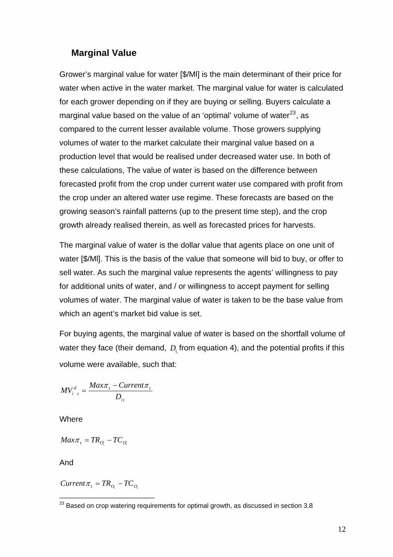
Marginal Value

Grower’s marginal value for water [$/Ml] is the main determinant of their price for

water when active in the water market. The marginal value for water is calculated

for each grower depending on if they are buying or selling. Buyers calculate a

marginal value based on the value of an ‘optimal’ volume of water23, as

compared to the current lesser available volume. Those growers supplying

volumes of water to the market calculate their marginal value based on a

production level that would be realised under decreased water use. In both of

these calculations, The value of water is based on the difference between

forecasted profit from the crop under current water use compared with profit from

the crop under an altered water use regime. These forecasts are based on the

growing season’s rainfall patterns (up to the present time step), and the crop

growth already realised therein, as well as forecasted prices for harvests.

The marginal value of water is the dollar value that agents place on one unit of

water [$/Ml]. This is the basis of the value that someone will bid to buy, or offer to

sell water. As such the marginal value represents the agents’ willingness to pay

for additional units of water, and / or willingness to accept payment for selling

volumes of water. The marginal value of water is taken to be the base value from

which an agent’s market bid value is set.

For buying agents, the marginal value of water is based on the shortfall volume of

water they face (their demand, from equation 4), and the potential profits if this

volume were available, such that:

tiD

ti

ttt

di D

CurrentMaxMV

ππ −=

Where

ii OOt TCTRMax ′′ −=π

And

ii OOt TCTRCurrent −=π

23 Based on crop watering requirements for optimal growth, as discussed in section 3.8

12

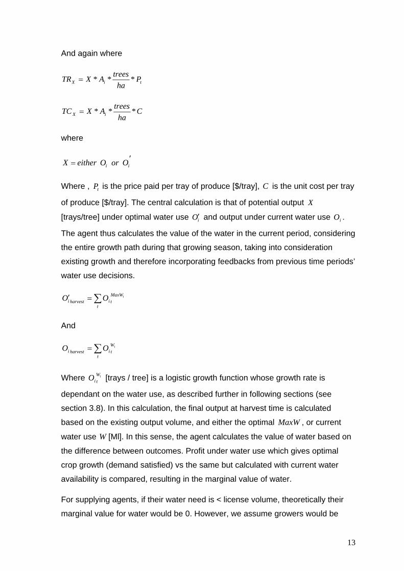
And again where

tiX Pha

treesAXTR ***=

Cha

treesAXTC iX ***=

where

′= ii OorOeitherX

Where , is the price paid per tray of produce [$/tray], C is the unit cost per tray

of produce [$/tray]. The central calculation is that of potential output

tP

X

[trays/tree] under optimal water use iO′ and output under current water use .

The agent thus calculates the value of the water in the current period, considering

the entire growth path during that growing season, taking into consideration

existing growth and therefore incorporating feedbacks from previous time periods’

water use decisions.

iO

∑=′t

tiharvestiiOO MaxW

W

W

And

∑=t

tiharvestiiOO

Where [trays / tree] is a logistic growth function whose growth rate is

dependant on the water use, as described further in following sections (see

section 3.8). In this calculation, the final output at harvest time is calculated

based on the existing output volume, and either the optimal , or current

water use W [Ml]. In this sense, the agent calculates the value of water based on

the difference between outcomes. Profit under water use which gives optimal

crop growth (demand satisfied) vs the same but calculated with current water

availability is compared, resulting in the marginal value of water.

itiO

MaxW

For supplying agents, if their water need is < license volume, theoretically their

marginal value for water would be 0. However, we assume growers would be

13

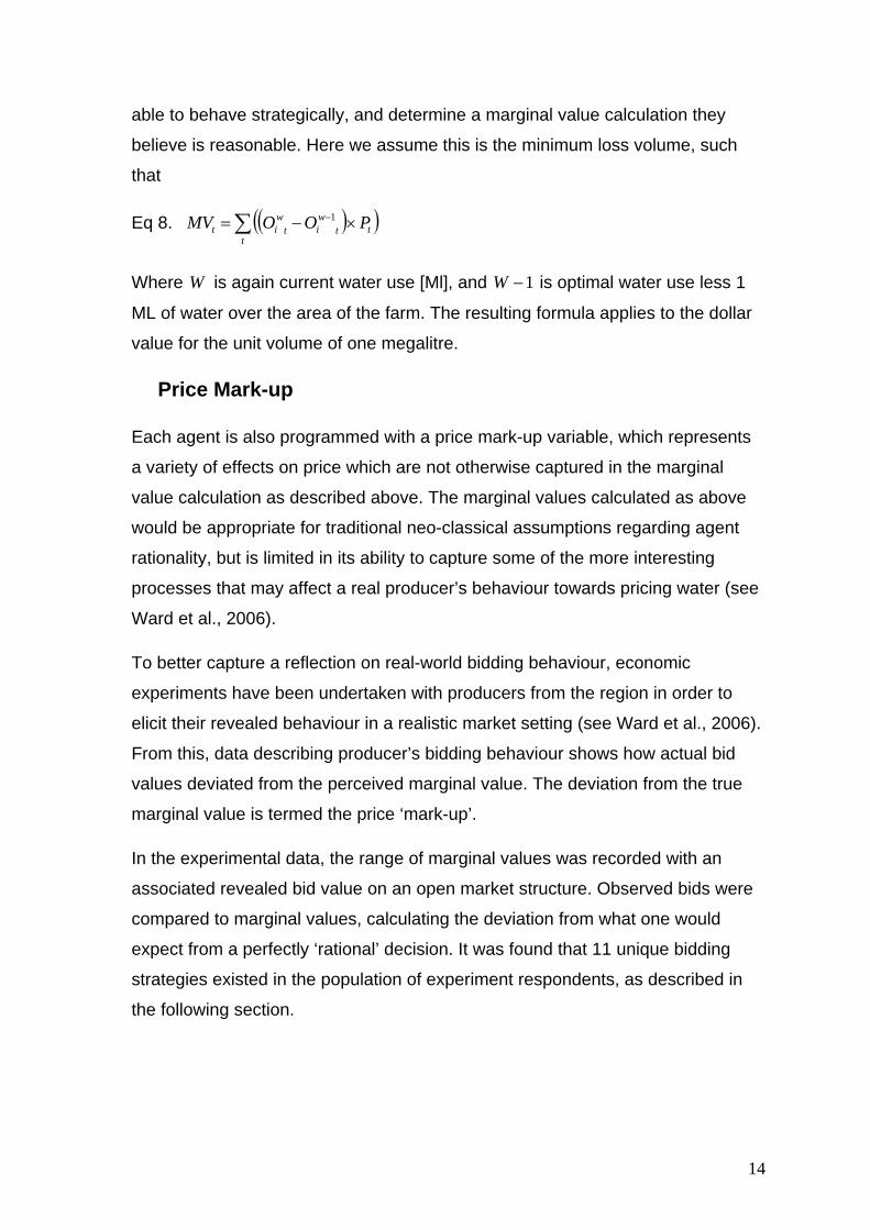
able to behave strategically, and determine a marginal value calculation they

believe is reasonable. Here we assume this is the minimum loss volume, such

that

(( ) )∑ ×−=t

ttitit POOMV −ww 1 Eq 8.

Where W is again current water use [Ml], and 1−W is optimal water use less 1

ML of water over the area of the farm. The resulting formula applies to the dollar

value for the unit volume of one megalitre.

Price Mark-up

Each agent is also programmed with a price mark-up variable, which represents

a variety of effects on price which are not otherwise captured in the marginal

value calculation as described above. The marginal values calculated as above

would be appropriate for traditional neo-classical assumptions regarding agent

rationality, but is limited in its ability to capture some of the more interesting

processes that may affect a real producer’s behaviour towards pricing water (see

Ward et al., 2006).

To better capture a reflection on real-world bidding behaviour, economic

experiments have been undertaken with producers from the region in order to

elicit their revealed behaviour in a realistic market setting (see Ward et al., 2006).

From this, data describing producer’s bidding behaviour shows how actual bid

values deviated from the perceived marginal value. The deviation from the true

marginal value is termed the price ‘mark-up’.

In the experimental data, the range of marginal values was recorded with an

associated revealed bid value on an open market structure. Observed bids were

compared to marginal values, calculating the deviation from what one would

expect from a perfectly ‘rational’ decision. It was found that 11 unique bidding

strategies existed in the population of experiment respondents, as described in

the following section.

14

Experimentally-calibrated Bidding Behaviour

Two important values required for the model in this second stage of the process

are the first bid value, and the adaptation of the agent’s bids as price signals are

perceived. The available options to parameterise these values include secondary

literature, expert opinion and historic data from other regions. Here we

parameterise the behaviour of simulated growers based on data from a series of

field experiments, discussed further in the next section. As such, decision making

behaviours were elicited using experimental economics techniques with actual

growers in the Katherine-Daly region24.

The results of the economic experiments yielded data about the first bid and how

bidding behaviour changed over time. The bidding strategies of the workshop

participants are used to calibrate the bidding behaviour of agents in the model by

superimposing the range of marginal values observed in the experiments over

the range calculated for agents in the model. Eleven bidding strategies were

observed within the experiments, and were related to the marginal value of water

that experiment participants perceived, with a range of marginal values existing

within the participant population. Simulated agents also calculate their marginal

values for water (discussed further below), and their location within this range

was located and assigned the related bidding strategy from the field experiment

population.

The mark up for each agent’s first bid was calibrated from the differences

between workshop participants’ marginal values and their first bids revealed in

the field experiments. The further adaptation of growers’ strategies over time is

calibrated based on the identification of explicit rules that workshop participants

followed when changing their bids in response to their experiences in the market.

See Smajgl and Heckbert (2006) for further discussion on calibration from

experiment results. The 11 bidding strategies observed in the economic

experiments are as follows, and are summarised visually in the following

associated figures.

24 The sample population participating in the experiment is self selected.

15

Strategy 1 corresponds to agents within the range of the lowest observed

marginal value. Hence, it was in their best interest to only make offers to sell

water allocations to other bidders with potentially higher willingness to pay

values. It was observed that the selling offers using this strategy were set at a

constant rate of above the perceived marginal value.

22

23

23

24

24

25

25

26

Oct Nov Dec Jan Feb Mar Apr May Jun Jul Aug Sep

Month

Valu

e ($

)

Marginal Value

Buying Price

Selling PriceMarginal Value

Selling Price

Month Figure 4: Bidding Strategy 1: Consistent mark-up value for selling bids

Strategy 2 and strategy 3 again apply to only selling offers, and have an

increasing value based on the success of market transactions. If a transaction

occurs, the agent will proceed to raise the bid to the next highest level in an

attempt to gain more revenue in the following potential transaction. If a

transaction does not occur, they maintain their bid for 6 months. If still no

transaction has occurred at this time, the bid value goes back down to the next

lowest bid, repeating this process over time.

0

10

20

30

40

50

60

70

80

90


Month

Valu

e ($

)

Marginal Value

Buying Price


Selling Price

Figure 5: Strategy 2: Increasing mark-up value

16

0

10

20

30

40

50

60

70

80

90


Month

Valu

e ($

)Marginal Value

Buying Price

Sell ing PriceMarginal Value

Selling Price

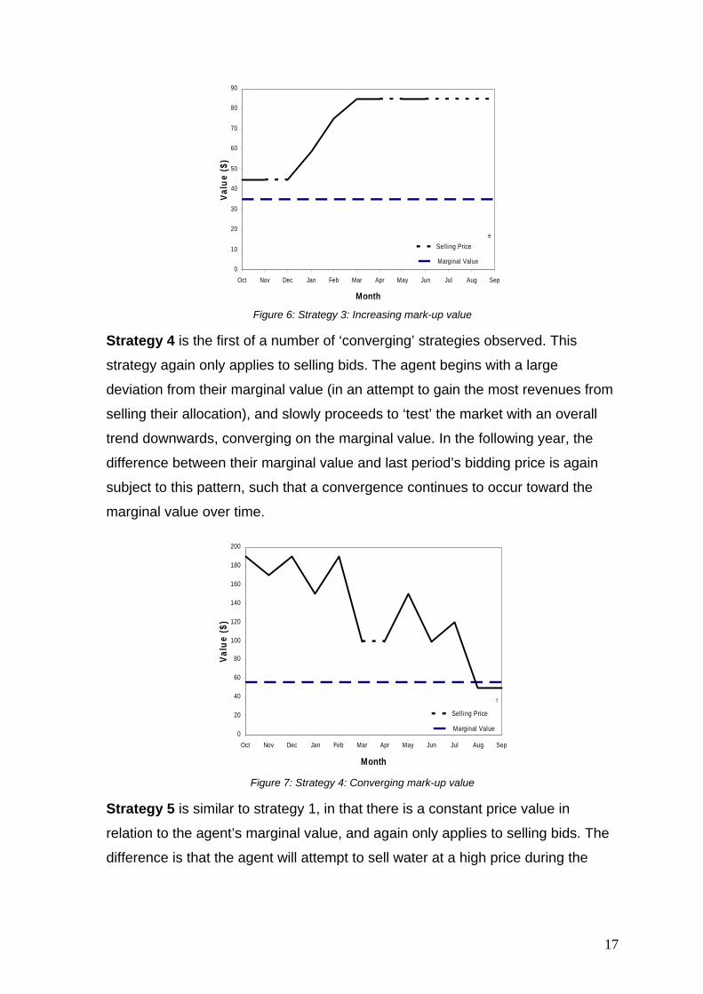
Figure 6: Strategy 3: Increasing mark-up value

Strategy 4 is the first of a number of ‘converging’ strategies observed. This

strategy again only applies to selling bids. The agent begins with a large

deviation from their marginal value (in an attempt to gain the most revenues from

selling their allocation), and slowly proceeds to ‘test’ the market with an overall

trend downwards, converging on the marginal value. In the following year, the

difference between their marginal value and last period’s bidding price is again

subject to this pattern, such that a convergence continues to occur toward the

marginal value over time.

0

20

40

60

80

100

120

140

160

180

200


Month

Valu

e ($

)

Marginal Value

Buying Price


Selling Price

Figure 7: Strategy 4: Converging mark-up value

Strategy 5 is similar to strategy 1, in that there is a constant price value in

relation to the agent’s marginal value, and again only applies to selling bids. The

difference is that the agent will attempt to sell water at a high price during the

17

periods where water demand is likely to be highest, and failing a successful

transaction, will revert to a lower value.

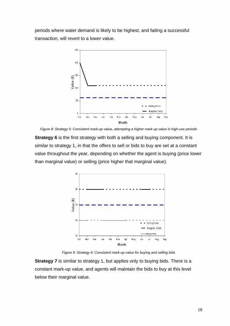
Figure 8: Strategy 5: Consistent mark-up value, attempting a higher mark up value in high-use periods

Strategy 6 is the first strategy with both a selling and buying component. It is

similar to strategy 1, in that the offers to sell or bids to buy are set at a constant

value throughout the year, depending on whether the agent is buying (price lower

than marginal value) or selling (price higher that marginal value).

Figure 9: Strategy 6: Consistent mark-up value for buying and selling bids

Strategy 7 is similar to strategy 1, but applies only to buying bids. There is a

constant mark-up value, and agents will maintain the bids to buy at this level

below their marginal value.

18

62

63

64

65


Month

Valu

e ($

)

Marginal Value

Buying Price

Selling Price

Figure 10: Strategy 7: Consistent mark-up value for buying bids

Strategy 8 Is a ‘double convergence’ strategy, in that the agent will make both

offers to sell or to buy. Each strategy converges eventually towards their marginal

value, in the same fashion described for strategy 4, above.

Figure 11: Strategy 8: Converging mark-up value for buying and selling bids

Strategy 9 is a buying only convergence strategy, similar to the prior

convergence strategies described, except that it was shown in the experimental

data that this agent overshot their ‘rational’ bidding value. Such behaviour

articulates that this individual perceived a higher value than the economic

marginal value communicated on the screen during the experiment. The strategy

overshoots the marginal value line, but re-converges from the other side.

19

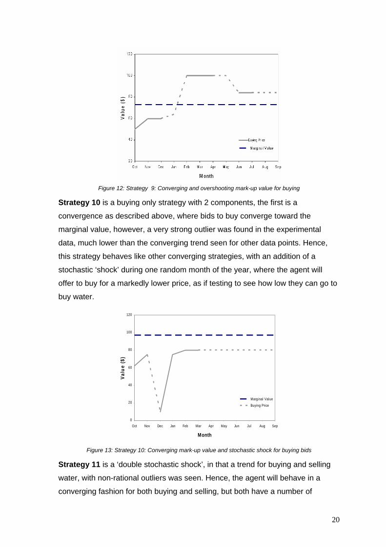
Figure 12: Strategy 9: Converging and overshooting mark-up value for buying

Strategy 10 is a buying only strategy with 2 components, the first is a

convergence as described above, where bids to buy converge toward the

marginal value, however, a very strong outlier was found in the experimental

data, much lower than the converging trend seen for other data points. Hence,

this strategy behaves like other converging strategies, with an addition of a

stochastic ‘shock’ during one random month of the year, where the agent will

offer to buy for a markedly lower price, as if testing to see how low they can go to

buy water.

0

20

40

60

80

100

120


Month

Valu

e ($

)

Marginal Value

Buying Price

Sell ing Price

Figure 13: Strategy 10: Converging mark-up value and stochastic shock for buying bids

Strategy 11 is a ‘double stochastic shock’, in that a trend for buying and selling

water, with non-rational outliers was seen. Hence, the agent will behave in a

converging fashion for both buying and selling, but both have a number of

20

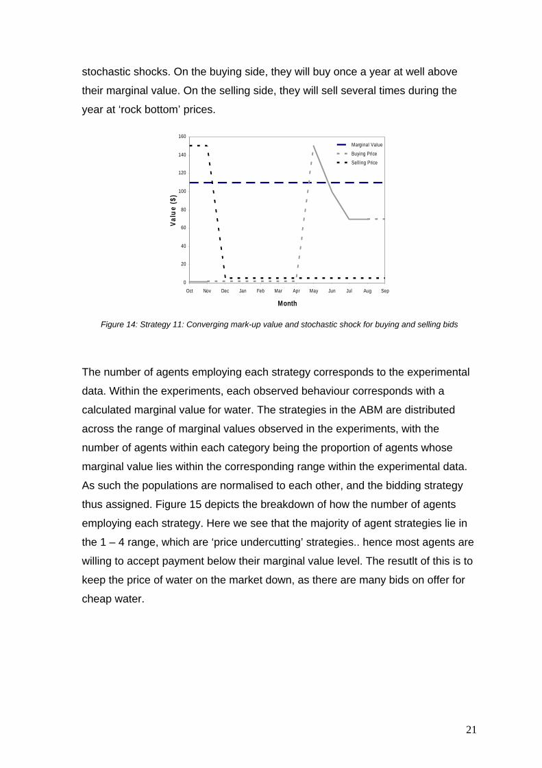
stochastic shocks. On the buying side, they will buy once a year at well above

their marginal value. On the selling side, they will sell several times during the

year at ‘rock bottom’ prices.

0

20

40

60

80

100

120

140

160


Month

Valu

e ($

)

Marginal Value

Buying Price

Selling Price

Figure 14: Strategy 11: Converging mark-up value and stochastic shock for buying and selling bids

The number of agents employing each strategy corresponds to the experimental

data. Within the experiments, each observed behaviour corresponds with a

calculated marginal value for water. The strategies in the ABM are distributed

across the range of marginal values observed in the experiments, with the

number of agents within each category being the proportion of agents whose

marginal value lies within the corresponding range within the experimental data.

As such the populations are normalised to each other, and the bidding strategy

thus assigned. Figure 15 depicts the breakdown of how the number of agents

employing each strategy. Here we see that the majority of agent strategies lie in

the 1 – 4 range, which are ‘price undercutting’ strategies.. hence most agents are

willing to accept payment below their marginal value level. The resutlt of this is to

keep the price of water on the market down, as there are many bids on offer for

cheap water.

21

Figure 15: Number of agents employing the eleven bidding strategies.

Market Structure

Producers can buy or sell water through posting offers to sell and/or bids to buy

volumes of water. The market structure is that of a double call market (see Ward

et al., 2006). To mimic the processes in this market structure, the process begins

with all agents who wish to place an offer to sell determining their desired selling

volume and price, as described above. Once all offers have been placed, agents

who wish to place a bid to buy water view the offers to sell.

An agent is randomly selected from the set of ‘buyers’, and views the offer of a

randomly selected ‘seller’. If the seller’s willingness to accept price is lower or

equal than buyer’s willingness to pay, the buyer purchases the volume of water

up to the their demanded volume. If the buyer purchases the seller’s entire supply

and has not fulfilled their demanded volume, the buyer proceeds to the next

seller’s offer and repeats the process.

Once the buyer has purchased their demanded volume or no offers to sell have a

sufficiently low price, the next buyer agent repeats the same process until all

demand is satisfied, all offers to sell are purchased, or no more transactions take

place due to discrepancies in buying and selling price. Once water is bought/sold,

the licensed water entitlements for the buyer and seller for that particular month

are updated. The buyer incurs a cost according to the seller’s offer price and

volume demanded, and the seller receives and associated revenue.

22

The market process is now complete for the given month, and agents realise their

actual water use levels, and the model may proceed to calculate the outcome of

the agents’ decisions.

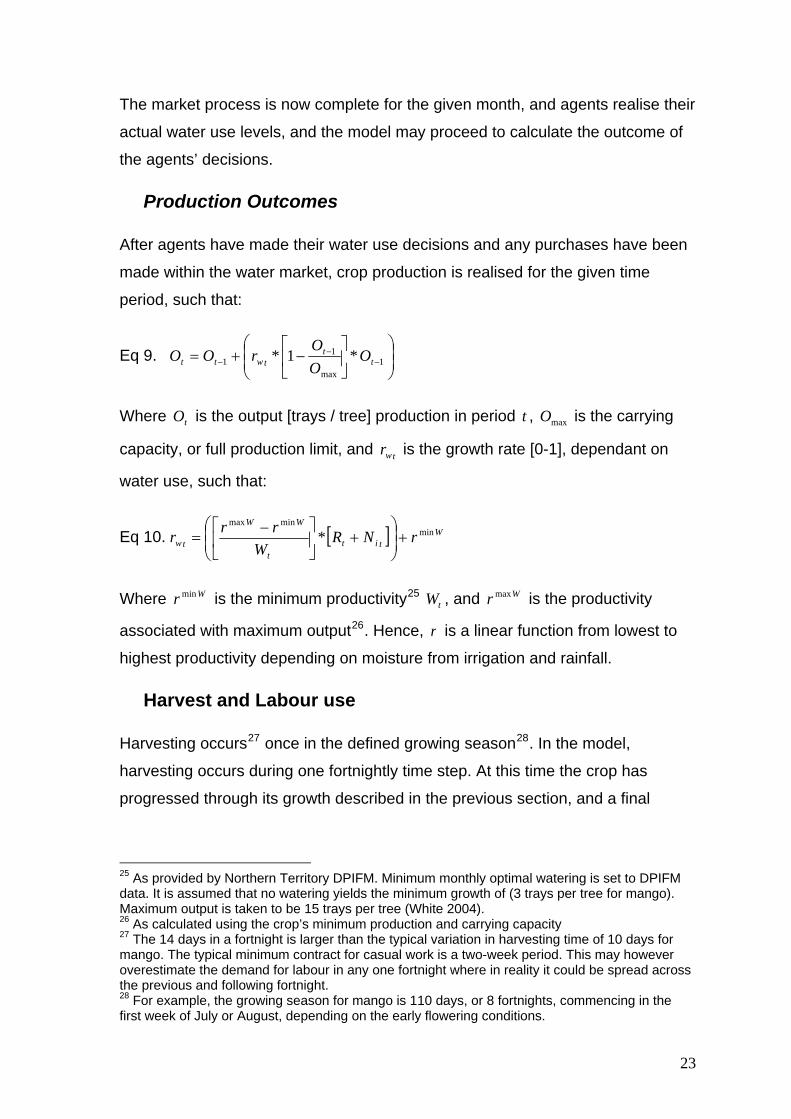
Production Outcomes

After agents have made their water use decisions and any purchases have been

made within the water market, crop production is realised for the given time

period, such that:

Eq 9. ⎟⎟⎠

⎞⎜⎜⎝

⎛⎥⎦

⎤⎢⎣

⎡−+= −

−− 1

max

11 *1* t

ttwtt O

OO

rOO

Where is the output [trays / tree] production in period , is the carrying

capacity, or full production limit, and is the growth rate [0-1], dependant on

water use, such that:

tO t maxO

twr

Eq 10. [ ] Wtit

t

WW

tw rNRW

rrr minminmax

* +⎟⎟⎠

⎞⎜⎜⎝

⎛+⎥

⎦

⎤⎢⎣

⎡ −=

Wr min W is the minimum productivity25 , and tW rWhere max is the productivity

associated with maximum output26. Hence, r is a linear function from lowest to

highest productivity depending on moisture from irrigation and rainfall.

Harvest and Labour use

Harvesting occurs27 once in the defined growing season28. In the model,

harvesting occurs during one fortnightly time step. At this time the crop has

progressed through its growth described in the previous section, and a final

25 As provided by Northern Territory DPIFM. Minimum monthly optimal watering is set to DPIFM data. It is assumed that no watering yields the minimum growth of (3 trays per tree for mango). Maximum output is taken to be 15 trays per tree (White 2004). 26 As calculated using the crop’s minimum production and carrying capacity 27 The 14 days in a fortnight is larger than the typical variation in harvesting time of 10 days for mango. The typical minimum contract for casual work is a two-week period. This may however overestimate the demand for labour in any one fortnight where in reality it could be spread across the previous and following fortnight. 28 For example, the growing season for mango is 110 days, or 8 fortnights, commencing in the first week of July or August, depending on the early flowering conditions.

23

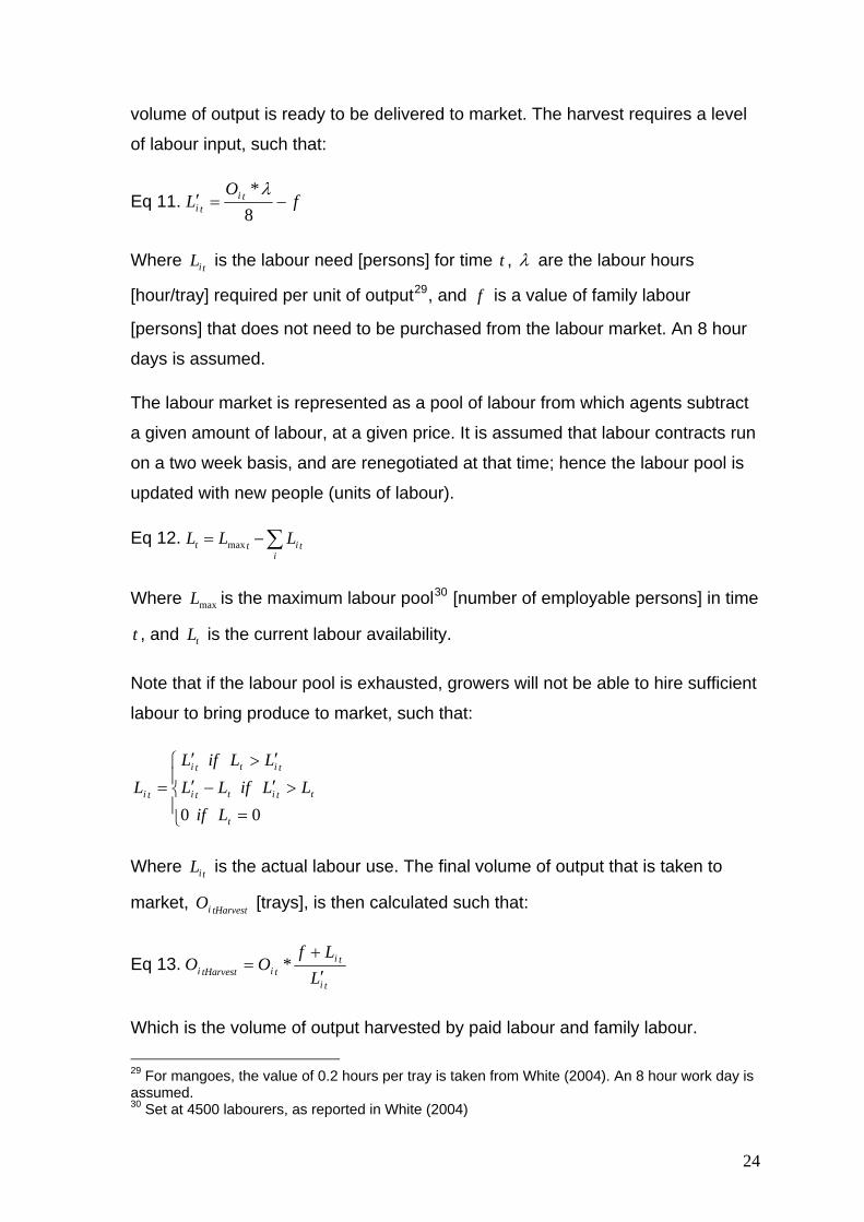
volume of output is ready to be delivered to market. The harvest requires a level

of labour input, such that:

Eq 11. fO

L titi −=′

8*λ

Where is the labour need [persons] for time t , tiL λ are the labour hours

[hour/tray] required per unit of output29, and is a value of family labour

[persons] that does not need to be purchased from the labour market. An 8 hour

days is assumed.

f

The labour market is represented as a pool of labour from which agents subtract

a given amount of labour, at a given price. It is assumed that labour contracts run

on a two week basis, and are renegotiated at that time; hence the labour pool is

updated with new people (units of labour).

Eq 12. ∑−=i

titt LLL max

Where is the maximum labour poolmaxL 30 [number of employable persons] in time

, and is the current labour availability. t tL

Note that if the labour pool is exhausted, growers will not be able to hire sufficient

labour to bring produce to market, such that:

⎪⎩

⎪⎨

⎧

=

>′−′

′>′

=

0 0

t

ttitti

titti

ti

LifLLifLL

LLifLL

Where is the actual labour use. The final volume of output that is taken to

market, [trays], is then calculated such that:

tiL

tHarvestiO

Eq 13. ti

tititHarvesti L

LfOO

′+

= *

Which is the volume of output harvested by paid labour and family labour.

29 For mangoes, the value of 0.2 hours per tray is taken from White (2004). An 8 hour work day is assumed. 30 Set at 4500 labourers, as reported in White (2004)

24

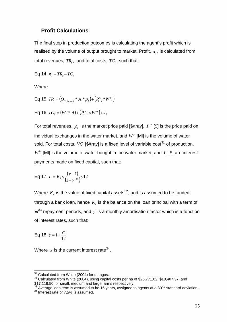
Profit Calculations

The final step in production outcomes is calculating the agent’s profit which is

realised by the volume of output brought to market. Profit, iπ , is calculated from

total revenues, , and total costs, , such that: iTR iTC

Eq 14. iii TCTR −=π

Where

Eq 15. ( ) ( )ttititHarvestii WPAOTR *** += ρ sw

Eq 16. ( ) ( ) itii IWPAVCTC +×+= * bw

For total revenues, tρ is the market price paid [$/tray], wP [$] is the price paid on

individual exchanges in the water market, and W [Ml] is the volume of water

sold. For total costs, VC [$/tray] is a fixed level of variable cost

s

b

31 of production,

[Ml] is the volume of water bought in the water market, and [$] are interest

payments made on fixed capital, such that:

W iI

( )( ) 121

1×

−−

×= −mii KIγ

γ Eq 17.

Where is the value of fixed capital assetsiK 32, and is assumed to be funded

through a bank loan, hence is the balance on the loan principal with a term of 33

iK

m repayment periods, and γ is a monthly amortisation factor which is a function

of interest rates, such that:

Eq 18. 12

1 αγ +=

Where α is the current interest rate34.

31 Calculated from White (2004) for mangos. 32 Calculated from White (2004), using capital costs per ha of $26,771.82, $18,407.37, and $17,119.50 for small, medium and large farms respectively. 33 Average loan term is assumed to be 15 years, assigned to agents at a 30% standard deviation. 34 Interest rate of 7.5% is assumed.

25

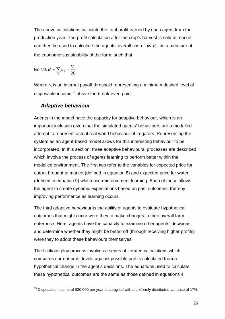
The above calculations calculate the total profit earned by each agent from the

production year. The profit calculation after the crop’s harvest is sold to market

can then be used to calculate the agents’ overall cash flow iθ , as a measure of

the economic sustainability of the farm, such that:

Eq 19. 26

i

ttit

V−=∑πθ

Where is an internal payoff threshold representing a minimum desired level of

disposable income

iV

35 above the break-even point.

Adaptive behaviour

Agents in the model have the capacity for adaptive behaviour, which is an

important inclusion given that the simulated agents’ behaviours are a modelled

attempt to represent actual real world behaviour of irrigators. Representing the

system as an agent-based model allows for this interesting behaviour to be

incorporated. In this section, three adaptive behavioural processes are described

which involve the process of agents learning to perform better within the

modelled environment. The first two refer to the variables for expected price for

output brought to market (defined in equation 8) and expected price for water

(defined in equation 9) which use reinforcement learning. Each of these allows

the agent to create dynamic expectations based on past outcomes, thereby

improving performance as learning occurs.

The third adaptive behaviour is the ability of agents to evaluate hypothetical

outcomes that might occur were they to make changes to their overall farm

enterprise. Here, agents have the capacity to examine other agents’ decisions,

and determine whether they might be better off (through receiving higher profits)

were they to adopt these behaviours themselves.

The fictitious play process involves a series of iterated calculations which

compares current profit levels against possible profits calculated from a

hypothetical change in the agent’s decisions. The equations used to calculate

these hypothetical outcomes are the same as those defined in equations 4

35 Disposable income of $30,000 per year is assigned with a uniformly distributed variance of 17%

26

through 20 above, as appropriate for the variables the agent is hypothetically

altering to explore potential outcomes.

The first step in fictitious play learning is to perceive behaviours or characteristics

of other agents. Within the model this is accomplished by agents exploring

options that are used by other, relatively profitable agents. Hence, if one agent is

receiving high payoffs, others will emulate their behaviour. However, in realty we

might not expect one producer to know the specific details about someone else’s

profit. Therefore it is not reasonable to simply allow simulated agents to have

open access to other agents’ profit levels. Nevertheless, someone making a

healthy profit is likely to ‘self-express’ their financial condition through a variety of

signals, such as making investment or purchasing goods that would otherwise be

out of reach for less financially successful agents. Therefore, simulated agents in

the model self-select to ‘flag’ themselves as having been successful if their profit

is relatively higher than the rest of the population, such that:

Eq 20. ( ) trueflag 1

n

n

2i

ii

i =⎯⎯ →⎯−

⎟⎟⎟⎟

⎠

⎞

⎜⎜⎜⎜

⎝

⎛

−

+>

∑∑

∑then

it

t

it

t nIf

ππ

ππ

Where the first element is the mean profit value, and the second element is the

standard deviation of profit across the population. In other words, if an agent’s

profit is greater than the average plus one standard deviation36, they ‘flag’

themselves as having been successful.

The possible adaptation strategies used here include:

• Change in off farm income –decreases family labour available for

production, increases off farm income

• Change production area – new areas under production, need to buy water

off market

• Exit market – sell water, no revenue from crop output, can pursue off farm

income

36 Normally distributed population, scores above the mean plus one standard deviation would amount to approximately 17% of the population.

27

• Change water use – buy or sell water on market, r in output is changed

Agents perform a series of iterated calculations to determine if any of the

adaptive strategies is expected to improve financial performance. If the option do

so, they are selected. Otherwise the agent continues the search until options are

selected, or exhausted.

4. Results Scenario 1: Baseline Conditions: No-trade , no new licenses

granted

The baseline scenario (n=18) describes the current licensing and extraction

situation on the Tindall aquifer. In this simulation, the original license holders are

simulated with their monthly allocations un-capped, and no water market exists

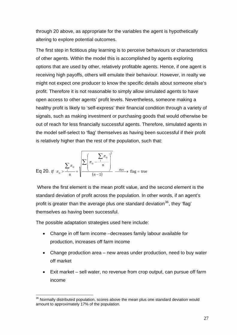
for trading. Fig. 16 shows results for total groundwater extraction (Ml) by

irrigators, annual rainfall (mm) and volume of groundwater available for extraction

(Ml). The historical rainfall data shows an initial period of abundant rain in years

1-6, followed by a number of dry years (approx 6 to 14) where rainfall levels are

not sufficient to fully recharge aquifer volumes. Rainfall again becomes generally

abundant from years 15 onward. Accordingly, extraction volumes correspond with

this pattern, with peaks in extraction matching low rainfall years.

0

200

400

600

800

1000

1200

1400

1600

1800

2000

1 2 3 4 5 6 7 8 9 10 11 12 13 14 15 16 17 18 19 20 21 22

Year

Tota

l Ann

ual R

ainf

all (

mm

)

0

1000

2000

3000

4000

5000

6000

Tota

l Ann

ual E

xtra

ctio

n (M

l)A

vaila

ble

Extr

actio

n Vo

lum

e (M

l)

)

)

Available extraction volumeTotal annual rainfallTotal annual extraction

(Ml)

Figure 16: Total groundwater extraction by irrigating growers, showing rainfall and available extraction

volumes, and the associated extraction levels for Scenario 1, showing baseline conditions.

28

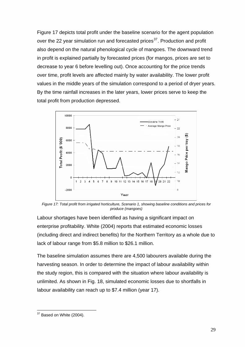
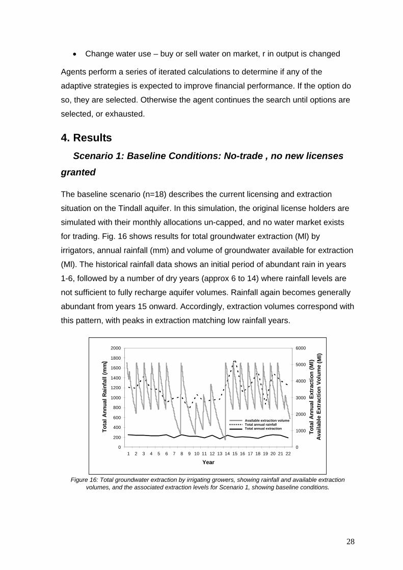
Figure 17 depicts total profit under the baseline scenario for the agent population

over the 22 year simulation run and forecasted prices37. Production and profit

also depend on the natural phenological cycle of mangoes. The downward trend

in profit is explained partially by forecasted prices (for mangos, prices are set to

decrease to year 6 before levelling out). Once accounting for the price trends

over time, profit levels are affected mainly by water availability. The lower profit

values in the middle years of the simulation correspond to a period of dryer years.

By the time rainfall increases in the later years, lower prices serve to keep the

total profit from production depressed.

Average Mango Price

Figure 17: Total profit from irrigated horticulture, Scenario 1, showing baseline conditions and prices for

produce (mangoes)

Labour shortages have been identified as having a significant impact on

enterprise profitability. White (2004) reports that estimated economic losses

(including direct and indirect benefits) for the Northern Territory as a whole due to

lack of labour range from $5.8 million to $26.1 million.

The baseline simulation assumes there are 4,500 labourers available during the

harvesting season. In order to determine the impact of labour availability within

the study region, this is compared with the situation where labour availability is

unlimited. As shown in Fig. 18, simulated economic losses due to shortfalls in

labour availability can reach up to $7.4 million (year 17).

37 Based on White (2004).

29

-2000

0

2000

4000

6000

8000

10000

12000

1 2 3 4 5 6 7 8 9 10 11 12 13 14 15 16 17 18 19 20 21 22

Year

Tota

l Pro

fit ($

'000

)

Unlimited LabourBaseline

Figure 18: Total profit under the baseline scenario compared to profit levels possible with unrestricted access

to labour. The distance between the two trajectories represents economic losses due to labour shortfalls.

0

1

2

3

1 2 3 4 5 6 7 8 9 10 11 12 13 14 15 16 17 18 19 20 21 22

Year

Gro

wer

s Se

ekin

g O

ff-fa

rm In

com

e

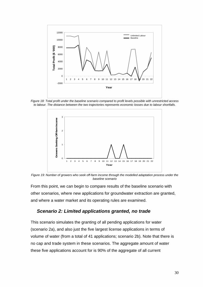
Figure 19: Number of growers who seek off-farm income through the modelled adaptation process under the

baseline scenario

From this point, we can begin to compare results of the baseline scenario with

other scenarios, where new applications for groundwater extraction are granted,

and where a water market and its operating rules are examined.

Scenario 2: Limited applications granted, no trade

This scenario simulates the granting of all pending applications for water

(scenario 2a), and also just the five largest license applications in terms of

volume of water (from a total of 41 applications; scenario 2b). Note that there is

no cap and trade system in these scenarios. The aggregate amount of water

these five applications account for is 90% of the aggregate of all current

30

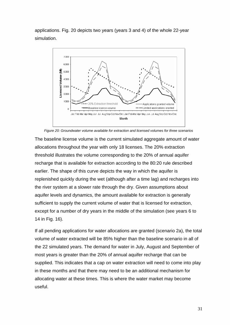
applications. Fig. 20 depicts two years (years 3 and 4) of the whole 22-year

simulation.

Figure 20: Groundwater volume available for extraction and licensed volumes for three scenarios

The baseline license volume is the current simulated aggregate amount of water

allocations throughout the year with only 18 licenses. The 20% extraction

threshold illustrates the volume corresponding to the 20% of annual aquifer

recharge that is available for extraction according to the 80:20 rule described

earlier. The shape of this curve depicts the way in which the aquifer is

replenished quickly during the wet (although after a time lag) and recharges into

the river system at a slower rate through the dry. Given assumptions about

aquifer levels and dynamics, the amount available for extraction is generally

sufficient to supply the current volume of water that is licensed for extraction,

except for a number of dry years in the middle of the simulation (see years 6 to

14 in Fig. 16).

If all pending applications for water allocations are granted (scenario 2a), the total

volume of water extracted will be 85% higher than the baseline scenario in all of

the 22 simulated years. The demand for water in July, August and September of

most years is greater than the 20% of annual aquifer recharge that can be

supplied. This indicates that a cap on water extraction will need to come into play

in these months and that there may need to be an additional mechanism for

allocating water at these times. This is where the water market may become

useful.

31

The result is similar when only the five largest volumetric applications for water

are granted (scenario 2b). Again, there is not sufficient extractable water to cover

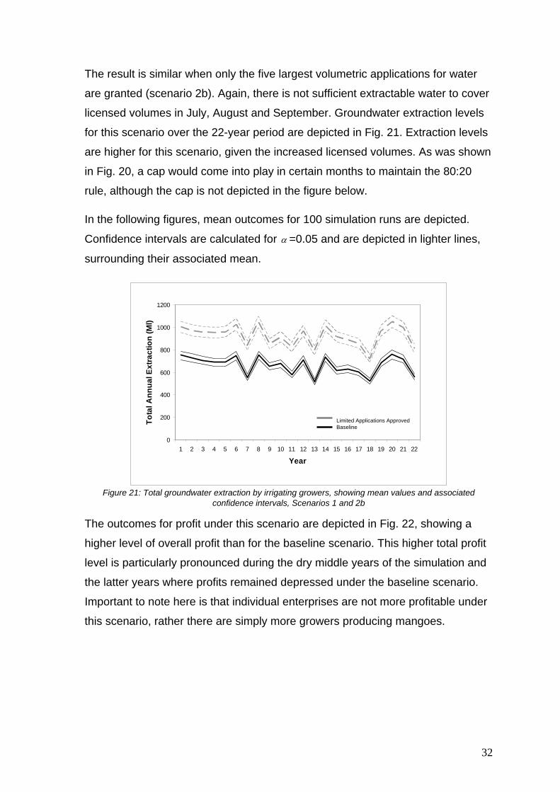
licensed volumes in July, August and September. Groundwater extraction levels

for this scenario over the 22-year period are depicted in Fig. 21. Extraction levels

are higher for this scenario, given the increased licensed volumes. As was shown

in Fig. 20, a cap would come into play in certain months to maintain the 80:20

rule, although the cap is not depicted in the figure below.

In the following figures, mean outcomes for 100 simulation runs are depicted.

Confidence intervals are calculated for α =0.05 and are depicted in lighter lines,

surrounding their associated mean.

0

200

400

600

800

1000

1200

1 2 3 4 5 6 7 8 9 10 11 12 13 14 15 16 17 18 19 20 21 22

Year

Tota

l Ann

ual E

xtra

ctio

n (M

l)

Limited Applications ApprovedBaseline

Figure 21: Total groundwater extraction by irrigating growers, showing mean values and associated

confidence intervals, Scenarios 1 and 2b

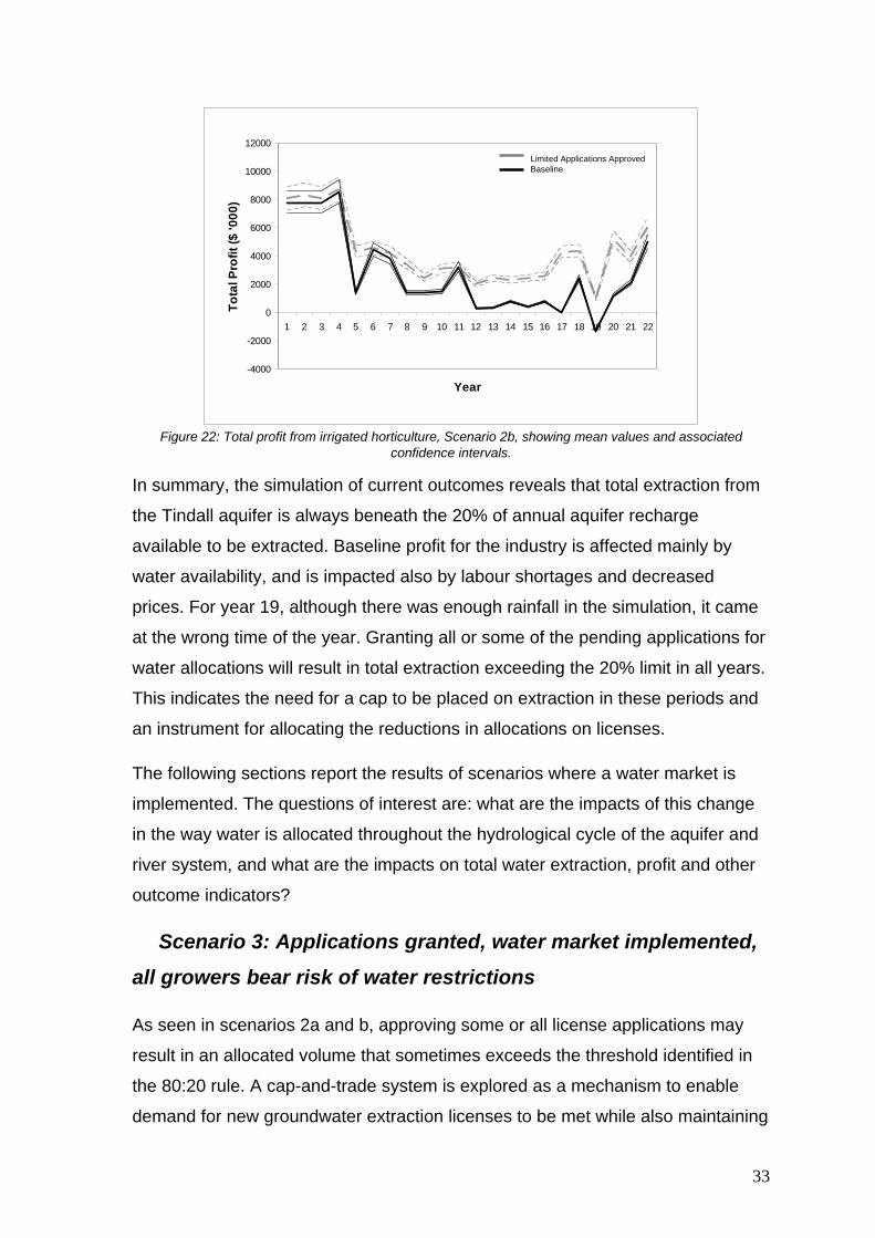
The outcomes for profit under this scenario are depicted in Fig. 22, showing a

higher level of overall profit than for the baseline scenario. This higher total profit

level is particularly pronounced during the dry middle years of the simulation and

the latter years where profits remained depressed under the baseline scenario.

Important to note here is that individual enterprises are not more profitable under

this scenario, rather there are simply more growers producing mangoes.

32

-4000

-2000

0

2000

4000

6000

8000

10000

12000

1 2 3 4 5 6 7 8 9 10 11 12 13 14 15 16 17 18 19 20 21 22

Year

Tota

l Pro

fit ($

'000

)

Limited Applications ApprovedBaseline

Figure 22: Total profit from irrigated horticulture, Scenario 2b, showing mean values and associated

confidence intervals.

In summary, the simulation of current outcomes reveals that total extraction from

the Tindall aquifer is always beneath the 20% of annual aquifer recharge

available to be extracted. Baseline profit for the industry is affected mainly by

water availability, and is impacted also by labour shortages and decreased

prices. For year 19, although there was enough rainfall in the simulation, it came

at the wrong time of the year. Granting all or some of the pending applications for

water allocations will result in total extraction exceeding the 20% limit in all years.

This indicates the need for a cap to be placed on extraction in these periods and

an instrument for allocating the reductions in allocations on licenses.

The following sections report the results of scenarios where a water market is

implemented. The questions of interest are: what are the impacts of this change

in the way water is allocated throughout the hydrological cycle of the aquifer and

river system, and what are the impacts on total water extraction, profit and other

outcome indicators?

Scenario 3: Applications granted, water market implemented,

all growers bear risk of water restrictions

As seen in scenarios 2a and b, approving some or all license applications may

result in an allocated volume that sometimes exceeds the threshold identified in

the 80:20 rule. A cap-and-trade system is explored as a mechanism to enable

demand for new groundwater extraction licenses to be met while also maintaining

33

environmental flows. Here, a market for trading water allocations is simulated,

and total water extraction is ‘capped’ when it reaches 20% of annual aquifer

recharge. Each individual license-holder must then face pumping restrictions of a

certain percentage of their monthly allocation.

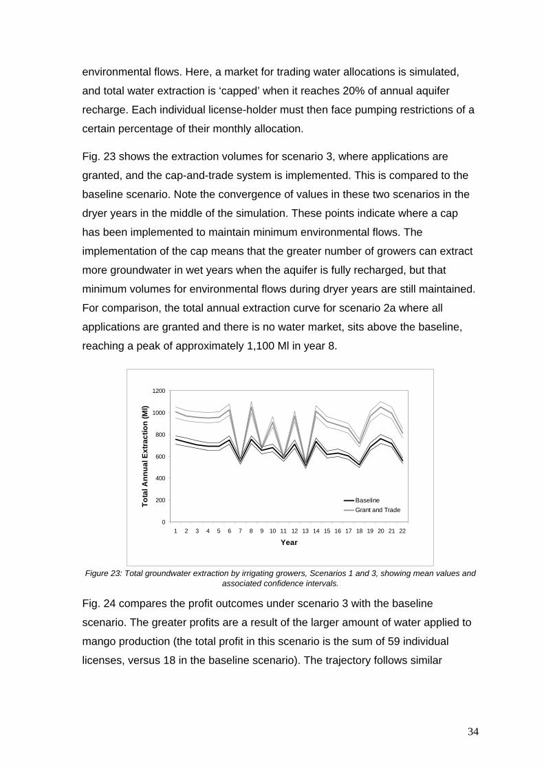
Fig. 23 shows the extraction volumes for scenario 3, where applications are

granted, and the cap-and-trade system is implemented. This is compared to the

baseline scenario. Note the convergence of values in these two scenarios in the

dryer years in the middle of the simulation. These points indicate where a cap

has been implemented to maintain minimum environmental flows. The

implementation of the cap means that the greater number of growers can extract

more groundwater in wet years when the aquifer is fully recharged, but that

minimum volumes for environmental flows during dryer years are still maintained.

For comparison, the total annual extraction curve for scenario 2a where all

applications are granted and there is no water market, sits above the baseline,

reaching a peak of approximately 1,100 Ml in year 8.

0

200

400

600

800

1000

1200

1 2 3 4 5 6 7 8 9 10 11 12 13 14 15 16 17 18 19 20 21 22

Year

Tota

l Ann

ual E

xtra

ctio

n (M

l)

BaselineGrant and Trade

Figure 23: Total groundwater extraction by irrigating growers, Scenarios 1 and 3, showing mean values and

associated confidence intervals.

Fig. 24 compares the profit outcomes under scenario 3 with the baseline

scenario. The greater profits are a result of the larger amount of water applied to

mango production (the total profit in this scenario is the sum of 59 individual

licenses, versus 18 in the baseline scenario). The trajectory follows similar

34

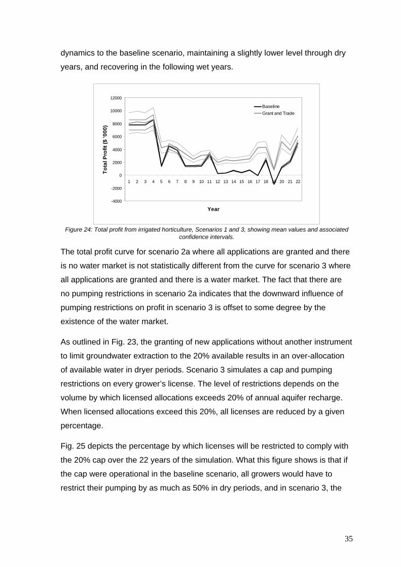
dynamics to the baseline scenario, maintaining a slightly lower level through dry

years, and recovering in the following wet years.

-4000

-2000

0

2000

4000

6000

8000

10000

12000

1 2 3 4 5 6 7 8 9 10 11 12 13 14 15 16 17 18 19 20 21 22

Year

Tota

l Pro

fit ($

'000

)BaselineGrant and Trade

Figure 24: Total profit from irrigated horticulture, Scenarios 1 and 3, showing mean values and associated


The total profit curve for scenario 2a where all applications are granted and there

is no water market is not statistically different from the curve for scenario 3 where

all applications are granted and there is a water market. The fact that there are

no pumping restrictions in scenario 2a indicates that the downward influence of

pumping restrictions on profit in scenario 3 is offset to some degree by the

existence of the water market.

As outlined in Fig. 23, the granting of new applications without another instrument

to limit groundwater extraction to the 20% available results in an over-allocation

of available water in dryer periods. Scenario 3 simulates a cap and pumping

restrictions on every grower’s license. The level of restrictions depends on the

volume by which licensed allocations exceeds 20% of annual aquifer recharge.

When licensed allocations exceed this 20%, all licenses are reduced by a given

percentage.

Fig. 25 depicts the percentage by which licenses will be restricted to comply with

the 20% cap over the 22 years of the simulation. What this figure shows is that if

the cap were operational in the baseline scenario, all growers would have to

restrict their pumping by as much as 50% in dry periods, and in scenario 3, the

35

cap is operational in the dry seasons of all years, and will require greater

pumping restrictions (up to 80%) in dryer years.

Figure 25: Percentage by which licenses will be restricted, Scenarios 1 and 3

The water market enables growers to purchase water subject to affordability and

availability in these highly restricted periods. Hence, while the cap manages

environmental risk, the market provides a mechanism for growers to manage

their own risk.

Fig. 26 depicts the volume of water demanded and supplied within the water

market under scenario 3. These trajectories again correspond with rainfall

patterns over the 22 year simulation. Note that Fig. 26 suggests that sufficient

supply of water allocations exists to meet demand in any given year.

0

500

1000

1500

2000

2500

1 2 3 4 5 6 7 8 9 10 11 12 13 14 15 16 17 18 19 20 21 22

Year

Wat

er D

eman

ded

(Ml)

Volume SuppliedVolume Demanded

Figure 26: Volume of water demanded and supplied within the water market, Scenario 3

36

Fig. 27 depicts the total volume of water purchased on the market (Ml) and the

bids, either to buy or to sell, made for water (note this is not the equilibrium price).

As would be expected, the volume purchased is higher when bids are lower and

vice versa. The spike in average bids made for water in the early years may

reflect that growers are learning about the water market and testing it out. The

lower points of volume purchased in years 10, 11 and 13 correspond to dryer

years, indicating that growers are trading less in these years. The lower volumes

purchased in years 2 to 4 may indicate that growers are learning about the

market in these years and increase their purchases as they become more familiar

with its operation. The volume of water purchased increases in later years of the

simulation as rainfall increases.

0

10

20

30

40

50

60

70

80

90

1 2 3 4 5 6 7 8 9 10 11 12 13 14 15 16 17 18 19 20 21 22

Year

Tota

l Vol

ume

Purc

hase

d (M

l)

0

50

100

150

200

250

300

350

Ave

rage

Wat

er P

rice

($)

Volume PurchasedWater Price

Ave

rage

bid

s m

ade

for w

ater

($/M

l)

Average bid

Figure 27: Volume purchased on the water market and average bid per Ml of water, Scenario 3

Fig. 28 illustrates the outcome of actual activity in the water market. Trading in

water allocations yields revenue ranging from less than $2,000 in year 18 up to

$10,000 in year 14. Here we see a level of trading of $7,000 to $10,000 in years

of higher rainfall, and depressed market activity in extremely dry years as

growers are less willing to part ways with their licensed volumes.

37

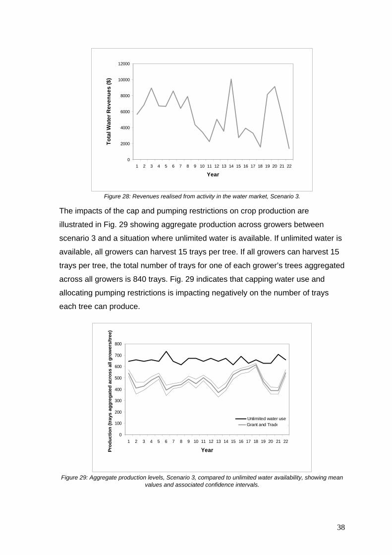
0

2000

4000

6000

8000

10000

12000

1 2 3 4 5 6 7 8 9 10 11 12 13 14 15 16 17 18 19 20 21 22

Year

Tota

l Wat

er R

even

ues

($)

Figure 28: Revenues realised from activity in the water market, Scenario 3.

The impacts of the cap and pumping restrictions on crop production are

illustrated in Fig. 29 showing aggregate production across growers between

scenario 3 and a situation where unlimited water is available. If unlimited water is

available, all growers can harvest 15 trays per tree. If all growers can harvest 15

trays per tree, the total number of trays for one of each grower’s trees aggregated

across all growers is 840 trays. Fig. 29 indicates that capping water use and

allocating pumping restrictions is impacting negatively on the number of trays

each tree can produce.

Unlimited water useNewcomers Bear BuGrant and Trade

0

100

200

300

400

500

600

700

800

1 2 3 4 5 6 7 8 9 10 11 12 13 14 15 16 17 18 19 20 21 22

Year

Prod

uctio

n (to

tal t

rays

/ tre

e)Pr

oduc

tion

(tray

s ag

greg

ated

acr

oss

all g

row

ers/

tree

)

Figure 29: Aggregate production levels, Scenario 3, compared to unlimited water availability, showing mean

values and associated confidence intervals.

38

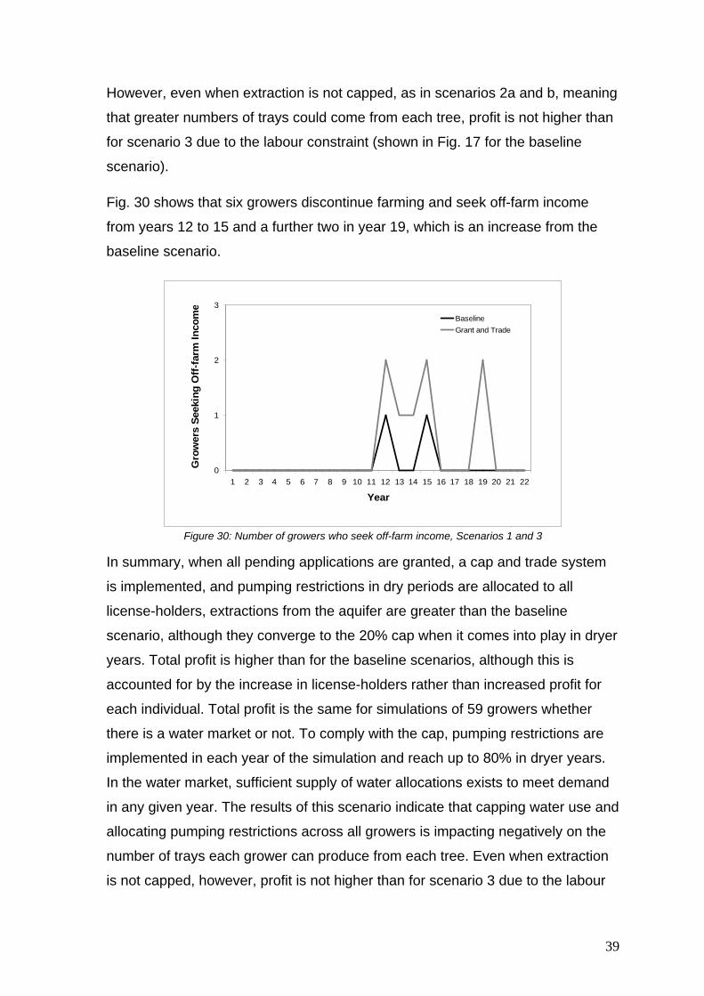
However, even when extraction is not capped, as in scenarios 2a and b, meaning

that greater numbers of trays could come from each tree, profit is not higher than

for scenario 3 due to the labour constraint (shown in Fig. 17 for the baseline

scenario).

Fig. 30 shows that six growers discontinue farming and seek off-farm income

from years 12 to 15 and a further two in year 19, which is an increase from the

baseline scenario.

0

1

2

3

1 2 3 4 5 6 7 8 9 10 11 12 13 14 15 16 17 18 19 20 21 22

Year

Gro

wer

s Se

ekin

g O

ff-f

arm

Inco

me

BaselineGrant and Trade

Figure 30: Number of growers who seek off-farm income, Scenarios 1 and 3

In summary, when all pending applications are granted, a cap and trade system

is implemented, and pumping restrictions in dry periods are allocated to all

license-holders, extractions from the aquifer are greater than the baseline

scenario, although they converge to the 20% cap when it comes into play in dryer

years. Total profit is higher than for the baseline scenarios, although this is

accounted for by the increase in license-holders rather than increased profit for

each individual. Total profit is the same for simulations of 59 growers whether

there is a water market or not. To comply with the cap, pumping restrictions are

implemented in each year of the simulation and reach up to 80% in dryer years.

In the water market, sufficient supply of water allocations exists to meet demand

in any given year. The results of this scenario indicate that capping water use and

allocating pumping restrictions across all growers is impacting negatively on the

number of trays each grower can produce from each tree. Even when extraction

is not capped, however, profit is not higher than for scenario 3 due to the labour

39

constraint. Therefore, both water and labour availability impact negatively on

profit. As a result of their observations of their own profits, eight growers exit the

industry in comparison to the two who leave in scenario 1.

The next scenario simulates the granting of all pending licenses, water trading

and allocates any pumping restrictions to new license-holders only rather than to

all.

Scenario 4: Applications granted, market created, newcomers

bear risk of pumping restrictions

A difficulty that exists in implementing a new policy mechanism such as a water

market is how to deal with people who have already been operating under the

previous policy regime, and whether to treat them differently to ‘newcomers’, who

enter the arena after changes are made. In this scenario we examine the

situation where pumping restrictions in dryer periods apply only to the

‘newcomers’ and existing license-holders may continue to use their pre-existing

allocated volumes without the risk of water restrictions being imposed.

Fig. 31 compares trajectories of extraction volumes for scenarios 3 and 4.

Scenario 4 sees an increase in groundwater extraction compared to scenario 3.

Existing license owners do not have their allocation capped. This means that in

some years the existing license owners extract all available water and this can

even exceed the 20% limit (as seen in the baseline curve of Fig. 25. This will

mean that in some years 0% of their licensed extraction is available to new

license holders. With a 20% cap imposed, even existing license-holders would

face restrictions of up to 50% in some years were the cap applicable to them as

well.

When the licensed extraction of all (existing and new) license holders exceeds

the 20% allowed then the burden of reduced allocation falls on the newcomers

and their allocation is reduced. This means that newcomers will rely more

heavily on water in the market to meet their desired water use.

40

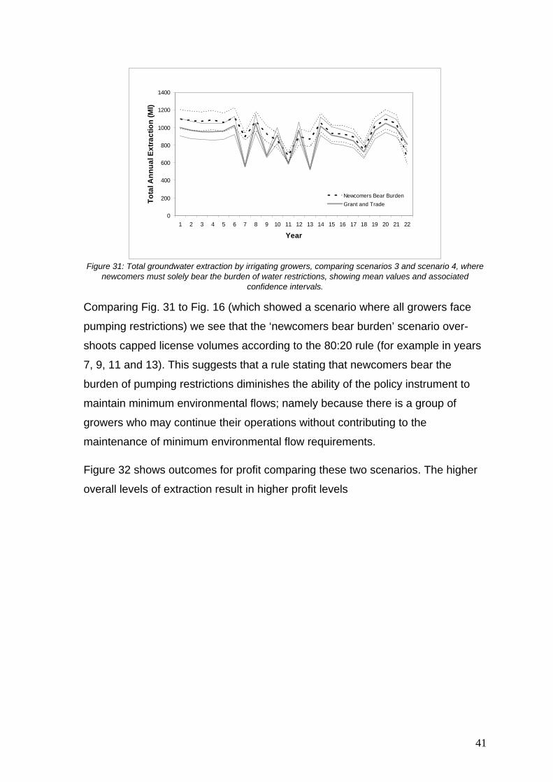
0

200

400

600

800

1000

1200

1400

1 2 3 4 5 6 7 8 9 10 11 12 13 14 15 16 17 18 19 20 21 22

Year

Tota

l Ann

ual E

xtra

ctio

n (M

l)

Newcomers Bear BurdenGrant and Trade

Figure 31: Total groundwater extraction by irrigating growers, comparing scenarios 3 and scenario 4, where

newcomers must solely bear the burden of water restrictions, showing mean values and associated confidence intervals.

Comparing Fig. 31 to Fig. 16 (which showed a scenario where all growers face

pumping restrictions) we see that the ‘newcomers bear burden’ scenario over-

shoots capped license volumes according to the 80:20 rule (for example in years

7, 9, 11 and 13). This suggests that a rule stating that newcomers bear the

burden of pumping restrictions diminishes the ability of the policy instrument to

maintain minimum environmental flows; namely because there is a group of

growers who may continue their operations without contributing to the

maintenance of minimum environmental flow requirements.

Figure 32 shows outcomes for profit comparing these two scenarios. The higher

overall levels of extraction result in higher profit levels

41

0

2000

4000

6000

8000

10000

12000

1 2 3 4 5 6 7 8 9 10 11 12 13 14 15 16 17 18 19 20 21 22

Year

Tota

l Pro

fit ($

'000

)


Figure 32: Profit from irrigated horticulture, Scenarios 3 and 4, showing mean values and associated


Fig. 33 depicts how this profit is distributed within the population of growers. The

Shannon Diversity Index38 reports on the distribution of profit within the

community of growers. A larger index value corresponds with a more even

distribution across agents. Comparing scenarios 3 and 4, we see approximately

four periods during simulation runs where the distribution of profit within the agent

population is significantly different between the two scenarios (approximately

years 9-10, 12-13, 16-17 and 18-21), particularly occurring in the middle dryer

years. The distribution of profit across growers starts more evenly and then

becomes less even.

38

⎟⎟⎟⎟

⎠

⎞

⎜⎜⎜⎜

⎝

⎛

⎟⎟⎟⎟

⎠

⎞

⎜⎜⎜⎜

⎝

⎛

−=∑∑i

i

i

ii

iSπ

ππ

πlog1*

where π is profit [$] realised at the end of harvest.

42

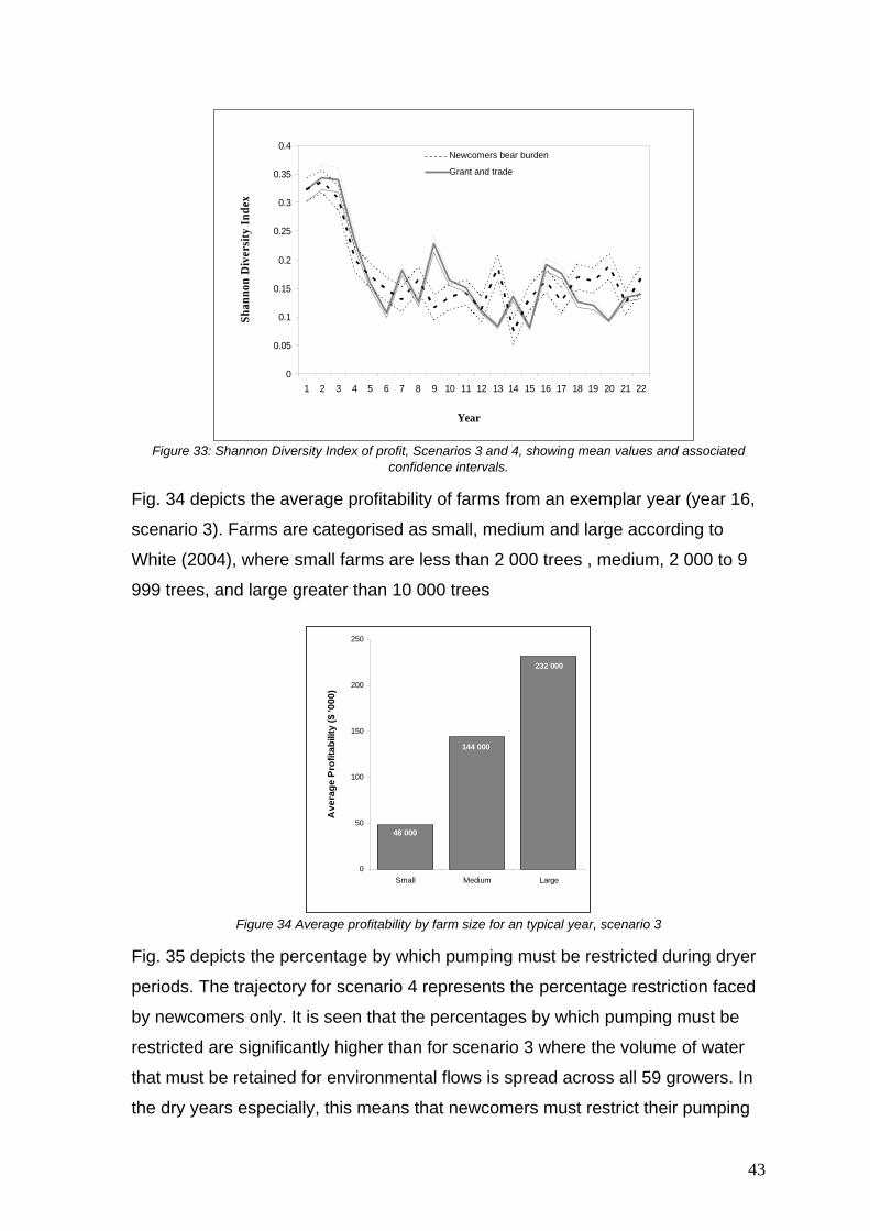
0

0.05

0.1

0.15

0.2

0.25

0.3

0.35

0.4

1 2 3 4 5 6 7 8 9 10 11 12 13 14 15 16 17 18 19 20 21 22

Year

Shan

non

Div

ersi

ty I

ndex

Newcomers bear burden

Grant and trade

Figure 33: Shannon Diversity Index of profit, Scenarios 3 and 4, showing mean values and associated


Fig. 34 depicts the average profitability of farms from an exemplar year (year 16,

scenario 3). Farms are categorised as small, medium and large according to

White (2004), where small farms are less than 2 000 trees , medium, 2 000 to 9

999 trees, and large greater than 10 000 trees

0

50

100

150

200

250

Small Medium Large

Ave

rage

Pro

fitab

ility

($ '0

00)

48 000

144 000

232 000

Figure 34 Average profitability by farm size for an typical year, scenario 3

Fig. 35 depicts the percentage by which pumping must be restricted during dryer

periods. The trajectory for scenario 4 represents the percentage restriction faced

by newcomers only. It is seen that the percentages by which pumping must be

restricted are significantly higher than for scenario 3 where the volume of water

that must be retained for environmental flows is spread across all 59 growers. In

the dry years especially, this means that newcomers must restrict their pumping

43

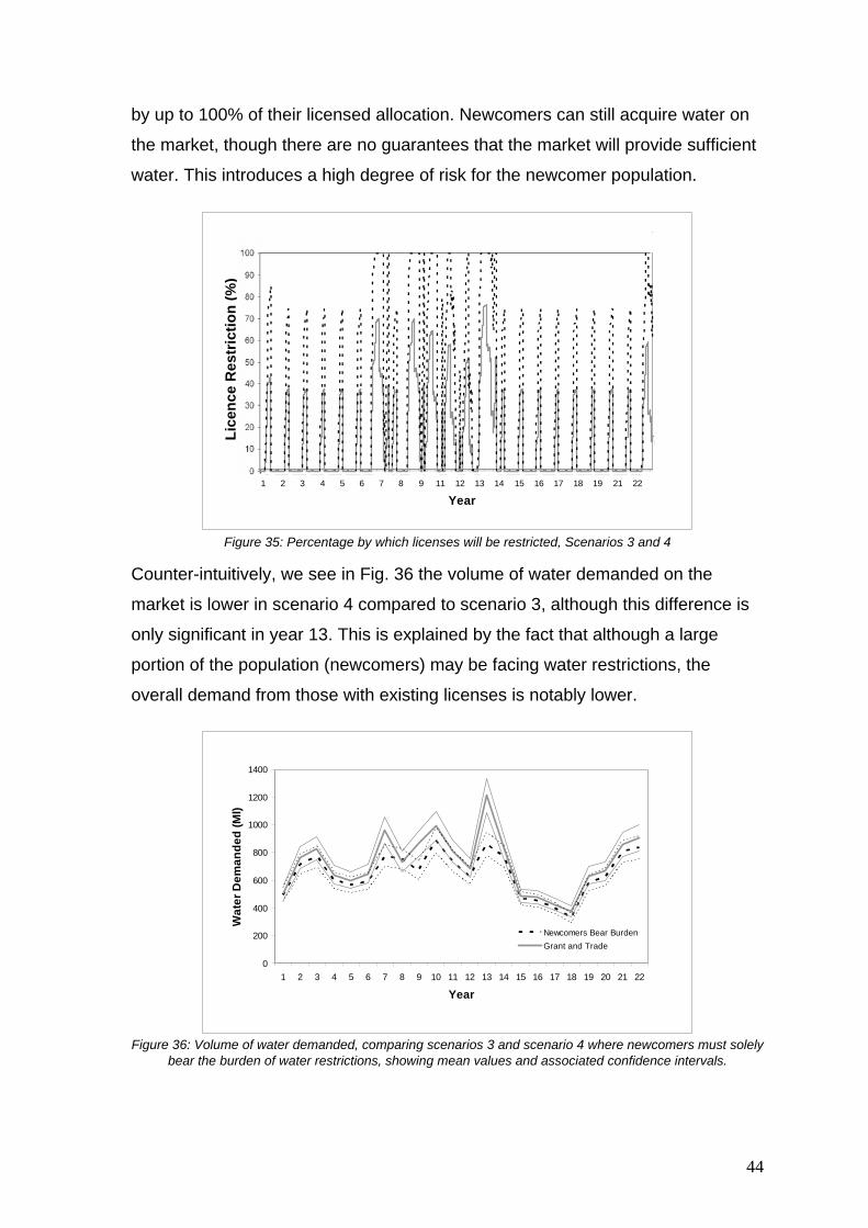
by up to 100% of their licensed allocation. Newcomers can still acquire water on

the market, though there are no guarantees that the market will provide sufficient

water. This introduces a high degree of risk for the newcomer population.

0

200

400

600

800

1000

1200

1 2 3 4 5 6 7 8 9 10 11 12 13 14 15 16 17 18 19 20 21 22

Year

Tota

l Ann

ual E

xtra

ctio

n (M

l)


Lice

nce

Res

tric

tion

(%)

0

0.1

0.2

0.3

0.4

0.5

0.6

0.7

0.8

0.9

1

1 2 3 4 5 6 7 8 9 11 12 13 14 15 16 17 18 19 21 22

()


Figure 35: Percentage by which licenses will be restricted, Scenarios 3 and 4

Counter-intuitively, we see in Fig. 36 the volume of water demanded on the

market is lower in scenario 4 compared to scenario 3, although this difference is

only significant in year 13. This is explained by the fact that although a large

portion of the population (newcomers) may be facing water restrictions, the

overall demand from those with existing licenses is notably lower.

0

200

400

600

800

1000

1200

1400

1 2 3 4 5 6 7 8 9 10 11 12 13 14 15 16 17 18 19 20 21 22

Year

Wat

er D

eman

ded

(Ml)


Figure 36: Volume of water demanded, comparing scenarios 3 and scenario 4 where newcomers must solely

bear the burden of water restrictions, showing mean values and associated confidence intervals.

44

As seen in Fig. 37, there is a significantly larger volume of water purchased on

the market in scenario 4 compared to scenario 3, less so but still pronounced in

the dryer years. Newcomers’ heavier reliance on the market results in higher

trading volumes.

0

20

40

60

80

100

120

140

1 2 3 4 5 6 7 8 9 10 11 12 13 14 15 16 17 18 19 20 21 22

Year

Tota

l Vol

ume

Purc

hase

d (M

l)


Grant and trade

Figure 37: Volume of water purchased in the market, Scenarios 3 and 4, showing mean values and


The volume of water supplied to the market is higher in scenario 4 compared to

scenario 3 although this difference is not statistically significant. This indicates

that existing license-holders are generally using the water they pump rather than

increasing their supply to the market substantially.

0

500

1000

1500

2000

2500

3000

1 2 3 4 5 6 7 8 9 10 11 12 13 14 15 16 17 18 19 20 21 22

Year

Wat

er S

uppl

ied

(Ml)


Figure 38: Volume of water supplied to the market, Scenarios 3 and 4, showing mean values and associated


45

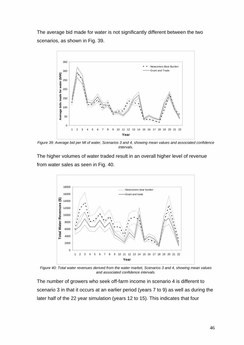
The average bid made for water is not significantly different between the two

scenarios, as shown in Fig. 39.

0

50

100

150

200

250

300

350

1 2 3 4 5 6 7 8 9 10 11 12 13 14 15 16 17 18 19 20 21 22

Year

Ave

rage

Wat

er P

rice

($)


Ave

rage

bid

s m

ade

for w

ater

($/M

l)

Figure 39: Average bid per Ml of water, Scenarios 3 and 4, showing mean values and associated confidence

intervals.

The higher volumes of water traded result in an overall higher level of revenue

from water sales as seen in Fig. 40.

0

2000

4000

6000

8000

10000

12000

14000

16000

18000

1 2 3 4 5 6 7 8 9 10 11 12 13 14 15 16 17 18 19 20 21 22

Year

Tota

l Wat

er R

even

ues

($)


Grant and trade

Figure 40: Total water revenues derived from the water market, Scenarios 3 and 4, showing mean values

and associated confidence intervals.

The number of growers who seek off-farm income in scenario 4 is different to

scenario 3 in that it occurs at an earlier period (years 7 to 9) as well as during the

later half of the 22 year simulation (years 12 to 15). This indicates that four

46

people exit the industry almost as soon as the dryer years in the middle of the 22-

year simulation begin rather than at the later stage as for scenario 3.

0

1

2

3

1 2 3 4 5 6 7 8 9 10 11 12 13 14 15 16 17 18 19 20 21 22

Year

Gro

wer

s Se

ekin

g O

ff-fa

rm In

com

eNewcomers Bear BurdenGrant and Trade

Figure 41: Number of growers who seek off-farm income, Scenarios 3 and 4

In summary, when only newcomers bear pumping restrictions, they can face

restrictions of up to 100% in some periods. Total water extraction from the aquifer

is higher in scenario 4 than scenario 3, meaning that the rule that only

newcomers bear pumping restrictions doesn’t enable the 20% limit on extraction

to be met, especially in dry years when newcomers face restrictions of up to

100%. Existing license-holders don’t necessarily supply more water to the

market, and more growers exit the industry earlier than for scenario 3.

Scenario 5: Applications granted, market created, trading

between east and west Tindall restricted

The final scenario considers the option of restricting trading in the region such

that there is no trading between growers extracting from the east side of the

Tindall aquifer and growers extracting from the west side of the Tindall aquifer.

The Katherine River is the approximate dividing line. In this scenario, growers on

the West Tindall may trade with other West Tindall growers, but not with growers

on the East Tindall area (and likewise for the other location). In this scenario, it is

seen that total extraction levels do not change compared to sceario 3, as shown

in Fig. 42.

47

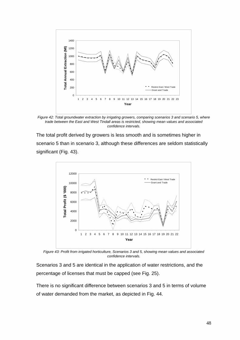
0

200

400

600

800

1000

1200

1400

1 2 3 4 5 6 7 8 9 10 11 12 13 14 15 16 17 18 19 20 21 22 23

Year

Tota

l Ann

ual E

xtra

ctio

n (M

l)

Newcomers Bear BurdenGrant and TradeRestrict East / West Trade

Figure 42: Total groundwater extraction by irrigating growers, comparing scenarios 3 and scenario 5, where

trade between the East and West Tindall areas is restricted, showing mean values and associated confidence intervals.

The total profit derived by growers is less smooth and is sometimes higher in

scenario 5 than in scenario 3, although these differences are seldom statistically

significant (Fig. 43).

0

2000

4000

6000

8000

10000

12000

1 2 3 4 5 6 7 8 9 10 11 12 13 14 15 16 17 18 19 20 21 22

Year

Tota

l Pro

fit ($

'000

)


Figure 43: Profit from irrigated horticulture, Scenarios 3 and 5, showing mean values and associated


Scenarios 3 and 5 are identical in the application of water restrictions, and the

percentage of licenses that must be capped (see Fig. 25).

There is no significant difference between scenarios 3 and 5 in terms of volume

of water demanded from the market, as depicted in Fig. 44.

48

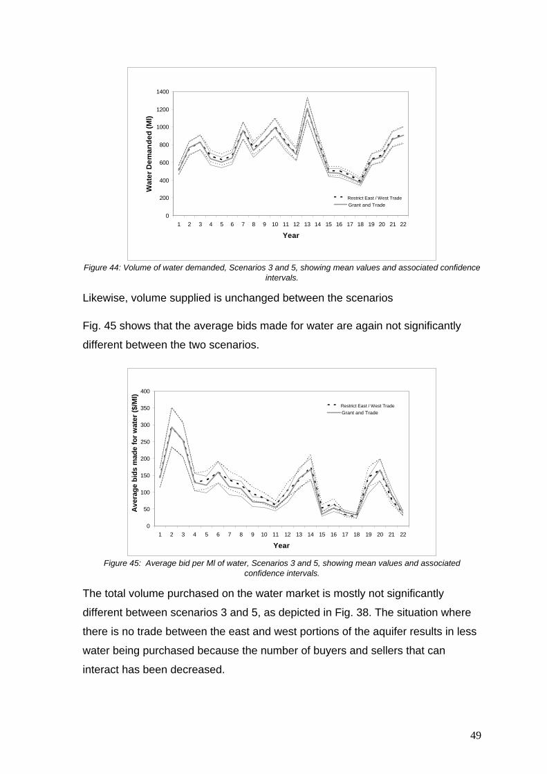
0

200

400

600

800

1000

1200

1400

1 2 3 4 5 6 7 8 9 10 11 12 13 14 15 16 17 18 19 20 21 22

Year

Wat

er D

eman

ded

(Ml)


Figure 44: Volume of water demanded, Scenarios 3 and 5, showing mean values and associated confidence

intervals.

Likewise, volume supplied is unchanged between the scenarios

Fig. 45 shows that the average bids made for water are again not significantly

different between the two scenarios.

0

50

100

150

200

250

300

350

400

1 2 3 4 5 6 7 8 9 10 11 12 13 14 15 16 17 18 19 20 21 22

Year

Ave

rage

Wat

er P

rice

($)


Ave

rage

bid

s m

ade

for w

ater

($/M

l)

Figure 45: Average bid per Ml of water, Scenarios 3 and 5, showing mean values and associated


The total volume purchased on the water market is mostly not significantly

different between scenarios 3 and 5, as depicted in Fig. 38. The situation where

there is no trade between the east and west portions of the aquifer results in less

water being purchased because the number of buyers and sellers that can

interact has been decreased.

49

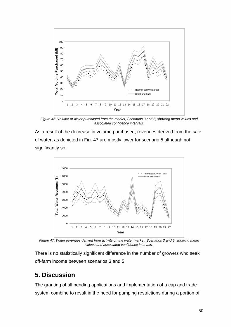
0

10

20

30

40

50

60

70

80

90

100

1 2 3 4 5 6 7 8 9 10 11 12 13 14 15 16 17 18 19 20 21 22

Year

Tota

l Vol

ume

Purc

hase

d (M

l)

Restrict east/west trade

Grant and trade

Figure 46: Volume of water purchased from the market, Scenarios 3 and 5, showing mean values and


As a result of the decrease in volume purchased, revenues derived from the sale

of water, as depicted in Fig. 47 are mostly lower for scenario 5 although not

significantly so.

0

2000

4000

6000

8000

10000

12000

14000

1 2 3 4 5 6 7 8 9 10 11 12 13 14 15 16 17 18 19 20 21 22

Year

Tota

l Wat

er R

even

ues

($)


Figure 47: Water revenues derived from activity on the water market, Scenarios 3 and 5, showing mean

values and associated confidence intervals.

There is no statistically significant difference in the number of growers who seek

off-farm income between scenarios 3 and 5.

5. Discussion The granting of all pending applications and implementation of a cap and trade

system combine to result in the need for pumping restrictions during a portion of

50

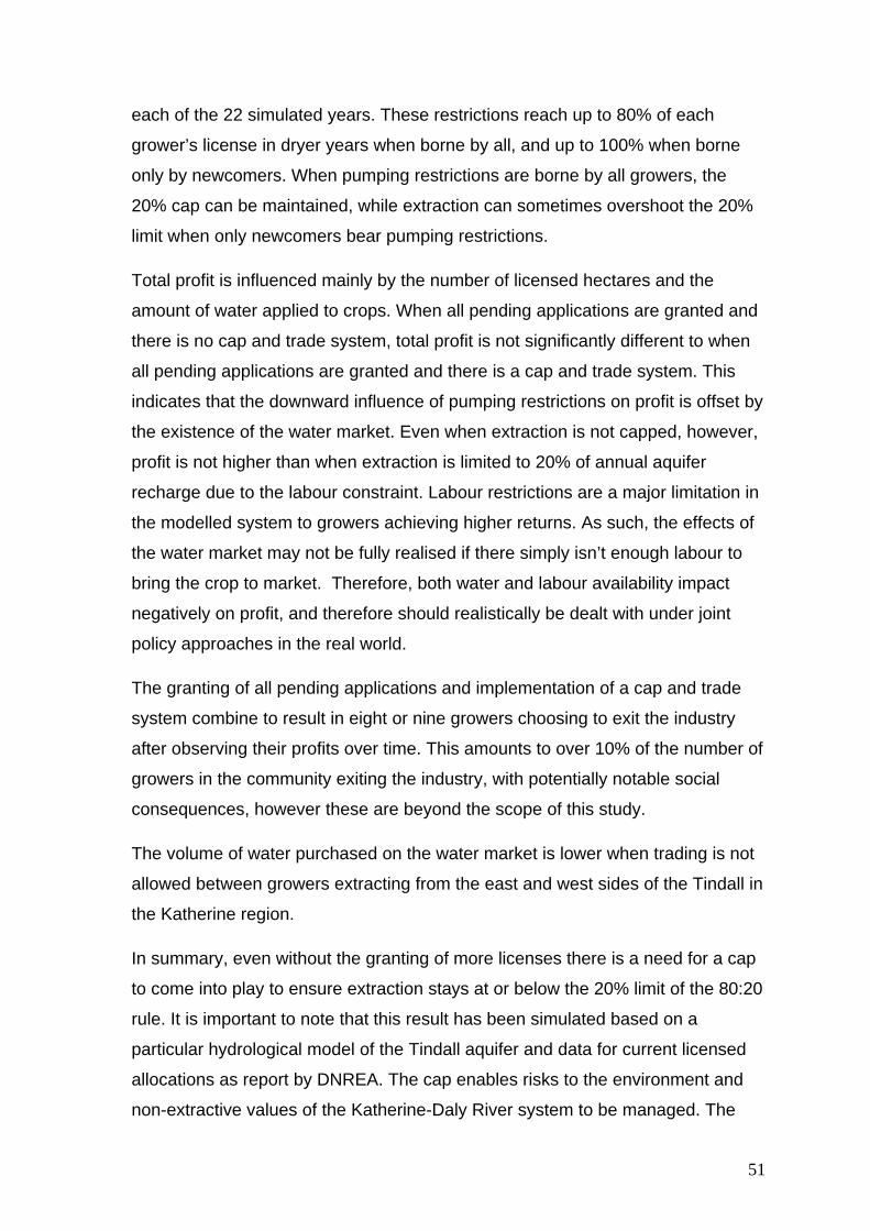
each of the 22 simulated years. These restrictions reach up to 80% of each

grower’s license in dryer years when borne by all, and up to 100% when borne

only by newcomers. When pumping restrictions are borne by all growers, the

20% cap can be maintained, while extraction can sometimes overshoot the 20%

limit when only newcomers bear pumping restrictions.

Total profit is influenced mainly by the number of licensed hectares and the

amount of water applied to crops. When all pending applications are granted and

there is no cap and trade system, total profit is not significantly different to when

all pending applications are granted and there is a cap and trade system. This

indicates that the downward influence of pumping restrictions on profit is offset by

the existence of the water market. Even when extraction is not capped, however,

profit is not higher than when extraction is limited to 20% of annual aquifer

recharge due to the labour constraint. Labour restrictions are a major limitation in

the modelled system to growers achieving higher returns. As such, the effects of

the water market may not be fully realised if there simply isn’t enough labour to

bring the crop to market. Therefore, both water and labour availability impact

negatively on profit, and therefore should realistically be dealt with under joint

policy approaches in the real world.

The granting of all pending applications and implementation of a cap and trade

system combine to result in eight or nine growers choosing to exit the industry

after observing their profits over time. This amounts to over 10% of the number of

growers in the community exiting the industry, with potentially notable social

consequences, however these are beyond the scope of this study.

The volume of water purchased on the water market is lower when trading is not

allowed between growers extracting from the east and west sides of the Tindall in

the Katherine region.

In summary, even without the granting of more licenses there is a need for a cap

to come into play to ensure extraction stays at or below the 20% limit of the 80:20

rule. It is important to note that this result has been simulated based on a

particular hydrological model of the Tindall aquifer and data for current licensed

allocations as report by DNREA. The cap enables risks to the environment and

non-extractive values of the Katherine-Daly River system to be managed. The

51

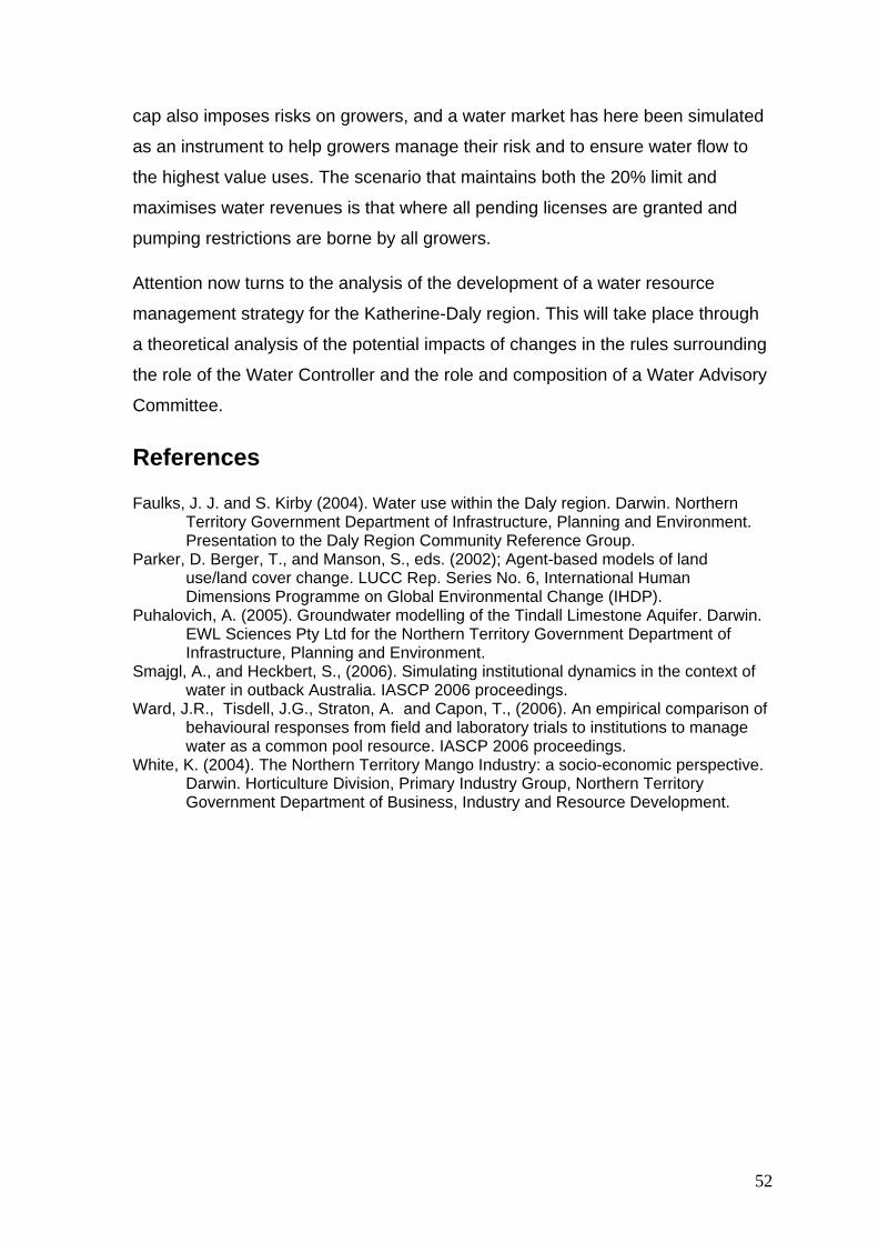
cap also imposes risks on growers, and a water market has here been simulated

as an instrument to help growers manage their risk and to ensure water flow to

the highest value uses. The scenario that maintains both the 20% limit and

maximises water revenues is that where all pending licenses are granted and

pumping restrictions are borne by all growers.

Attention now turns to the analysis of the development of a water resource

management strategy for the Katherine-Daly region. This will take place through

a theoretical analysis of the potential impacts of changes in the rules surrounding

the role of the Water Controller and the role and composition of a Water Advisory

Committee.

References Faulks, J. J. and S. Kirby (2004). Water use within the Daly region. Darwin. Northern

Territory Government Department of Infrastructure, Planning and Environment. Presentation to the Daly Region Community Reference Group.

Parker, D. Berger, T., and Manson, S., eds. (2002); Agent-based models of land use/land cover change. LUCC Rep. Series No. 6, International Human Dimensions Programme on Global Environmental Change (IHDP).

Puhalovich, A. (2005). Groundwater modelling of the Tindall Limestone Aquifer. Darwin. EWL Sciences Pty Ltd for the Northern Territory Government Department of Infrastructure, Planning and Environment.

Smajgl, A., and Heckbert, S., (2006). Simulating institutional dynamics in the context of water in outback Australia. IASCP 2006 proceedings.

Ward, J.R., Tisdell, J.G., Straton, A. and Capon, T., (2006). An empirical comparison of behavioural responses from field and laboratory trials to institutions to manage water as a common pool resource. IASCP 2006 proceedings.

White, K. (2004). The Northern Territory Mango Industry: a socio-economic perspective. Darwin. Horticulture Division, Primary Industry Group, Northern Territory Government Department of Business, Industry and Resource Development.

52

53 53

Tindall Aquifer Water Trading Model: Technical Report and Scenario Results

Documents