TIME-VARYING CONDITIONAL SKEWNESS AND … CONDITIONAL SKEWNESS AND THE MARKET RISK ... present time-series evidence that the expected market risk premium is, ... As shown in Harvey

TIME-VARYING CONDITIONALSKEWNESS AND THE MARKET RISKPREMIUM

Campbell R. Harvey and Akhtar Siddique

ABSTRACT

Single factor asset pricing models face two major hurdles: the problematictime-series properties of the ex ante market risk premium and the inabilityof the risk measure to account for a substantial degree of the cross-sectional variation of expected excess returns. We provide an explanationfor the first failure using the following intuition: if investors know that theasset returns have conditional skewness at time t, the expected excessreturns should include rewards for accepting skewness. We formalize thisintuition with an asset pricing model which incorporates conditionalskewness. We decompose the expected excess returns into components dueto conditional variance and skewness. Our results show that conditionalskewness is important and, when combined with the economy-wide rewardfor skewness, helps explain the time-variation of the ex ante market riskpremiums. Conditional skewness has greater success in explaining the exante risk premium for the world portfolio than for the U.S. portfolio.

1. INTRODUCTION

The behavior of the market risk premium in the Capital Asset Pricing Model(CAPM) of Sharpe (1964) and Lintner (1965) has come under scrutiny from

Research in Banking and Finance, Volume 1, pages 25–58.Copyright © 2000 by JAI/Elsevier Inc.All rights of reproduction in any form reserved.ISBN: 0-444-50587-3

25

two fronts. First, the evidence in Fama & French (1992) suggests that theestimated market risk premium is not different from zero. This implies that thesystematic risk of the CAPM is not rewarded. Second, Boudoukh, Richardson& Smith (1993) present time-series evidence that the expected market riskpremium is, at times, significantly less than zero. This implies that the marketportfolio is on the negatively sloped portion of the mean-variance frontier – aviolation of one of the CAPM’s restrictions.

Aside from the criticism related to the market risk premium, results fromcross-sectional tests of the single factor asset pricing model seem to indicatethat the cross-asset variation in expected returns can not be explained by themarket beta alone. For example, a number of recent papers find that‘fundamental’ factors, which are idiosyncratic in nature, account for a sizableportion of the cross-sectional variation in expected returns [see Fama & French(1992); Chan, Hamao & Lakonishok (1991)]. Harvey & Siddique (2000) findthat using conditional coskewness with the market can substantially mitigatethe shortcomings of the single factor asset pricing model in explaining thecross-sectional variations in expected returns.

This study focuses on the time-series behavior of the risk premium. Ourexplanation for the time-series behavior of the market risk premium relies upona single factor asset pricing model incorporating conditional skewness. Thisframework complements the cross-sectional results in Harvey & Siddique(2000).

Several important distinctions exist between our results and other recentwork. In contrast to the usual beta-risk premium decomposition, we identify therisk factors in terms of the higher conditional moments such as the conditionalcovariance with the market and the conditional coskewness with the market.The second difference is in our use of a conditional methodology. We explicitlyassume that the investor’s information set changes over time. Thus, we allowtime-varying risk and prices of risk and capture the variation with economicallymeaningful instrumental variables.

The following is our intuition for including skewness in the asset pricingframework. In the usual setup, investors have preferences over the mean andthe variance of portfolio returns. The systematic risk of a security is measuredas the contribution to the variance of a well-diversified portfolio. However,there is considerable evidence that the returns distributions cannot beadequately characterized by mean and variance alone. This leads us to nextmoment – skewness. Given the statistical evidence of skewness in returns, it isreasonable to assume that investors have preferences for skewness. With a largepositive skewness (high probability of a large positive return), the investorsmay be willing to hold a portfolio even if its expected return is negative. As we

26 CAMPBELL R. HARVEY & AKHTAR SIDDIQUE

show later, this is still fully consistent with the Arrow-Pratt notion of riskaversion. Similarly, variation in skewness risk should also be important for thecross-section of assets.

Skewness may be important in investment decisions because of inducedasymmetries in ex-post (realized) returns. At least two factors may induceasymmetries. First, the presence of limited liability in all equity investmentsmay induce option-like asymmetries in returns [see Black (1976), Christie(1982) and Nelson (1991)]. Second, the agency problem may induceasymmetries in index returns [see Brennan (1993)]. That is, a manager has acall option with respect to the outcome of his investment strategies. Managersmay prefer portfolios with high positive skewness.

We present an asset pricing model where skewness is priced. Ourformulation is related to the seminal work of Kraus & Litzenberger (1976) andmore recently, to the nonlinear factor model presented in Bansal &Viswanathan (1993). Our evidence documents significant time-variation inconditional skewness measures for both the U.S. stock market and, a broaderworld market portfolio. We estimate the price of skewness risk and show thatthis asset pricing model can account for much of the time-series variation in theexpected market risk premium. We also find that this model helps explain manyof the episodes of negative ex ante market risk premiums.

Our chapter is organized as follows. In the second Section, we use a generalstochastic discount factor pricing framework to show how skewness can affectthe expected market risk premia. Our econometric methodology and tests aredetailed in the third Section. The data are described in this Section as well. Theempirical results for the market risk premium are described in the fourthSection. The final part offers some concluding remarks.

2. SKEWNESS IN ASSET PRICING THEORY

The first-order condition for an investor holding a risky asset for one periodis:

E[(1 + Ri,t+1)mt+1|�t] = 1 (1)

where (1 + Ri,t+1) is the total return on asset i, mt+1 is the marginal rate ofsubstitution of the investor between periods t and t + 1, and �t is theinformation set available to the investor at time t. mt+1 can be viewed as apricing kernel or a stochastic discount factor that prices all risky asset payoffs.

As shown in Harvey & Siddique (2000), assuming a linear functional formfor the marginal rate of substitution

mt+1 = at + btRM,t+1, (2)

27Skewness and the Market Risk Premium

and the existence of a riskfree asset, we get the standard CAPM

Et[ri,t+1] =Et[rM,t+1]

Vart[rM,t+1]Covt[ri,t+1,rM,t+1] (3)

where lower case r represents returns of a conditionally riskfree return. In sucha model, the expected excess returns of the risky assets are independent of thespanning weights at and bt.

The expression for the market risk premium, however, does incorporate, thespanning weights since

Et[rM,t+1] = � btRf,t+1Vart[rM,t+1] (4)

where Rf,t+1 is one plus the conditionally riskfree rate of return. Thus, theexpected market risk premium equals the conditional variance of the marketreturn multiplied by the price of variance risk. The price of market variance riskis simply the spanning weight bt inflated by � Rf,t+1. Temporal variation in theprice of variance risk comes from both Rf,t+1 and bt.

If we relate the discount factor to the marginal rate of substitution betweenperiods t and t + 1, a Taylor’s series expansion allows us to make the followingidentification:

mt+1 = 1 +WtU�(Wt)U�(Wt)

RM,t+1 + o(Wt)

where o(Wt) is the remainder in the expansion and WtU�(Wt)U�(Wt)

(which is � bt in

(2)) is relative risk aversion. Then at = 1 + o(Wt) and bt < 0. A negative bt

implies that with an increase in next period’s market return, the marginal rateof substitution declines. This decline in the marginal rate of substitution isconsistent with decreasing marginal utility. This restriction implies that theexpected market risk premium is positive. Even if we only observe a proxy forthe market, say portfolio r*m,t, a positive conditional covariance with the truemarket portfolio implies that the expected excess return on the proxy shouldalso be positive.

Departing from the standard approach and assuming that the stochasticdiscount factor is quadratic in the market return:

mt+1 = at + btRM,t+1 + ctR2M,t+1 (5)

gives us a model where the expected excess return on the asset is determinedby both its conditional covariance with the market return and with the squareof the market return (conditional coskewness). Again assuming the existence ofa conditionally riskfree asset:


Et[ri,t+1] =Vart[r

2M,t+1]Et[rM,t+1] � Skewt[rM,t+1]Et[r

2M,t+1]

Vart[rM,t+1]Vart[r2M,t+1] � Skewt[rM,t+1])

2 Covt[ri,t+1,rM,t+1],

+Vart[rM,t+1]Et[r

2M,t+1 � Skewt[rM,t+1]Et[rM,t+1]

Vart[rM,t+1]Vart[r2M,t+1] � (Skewt[rM,t+1])

2 Covt[ri,t+1,r2M,t+1]

. (6)

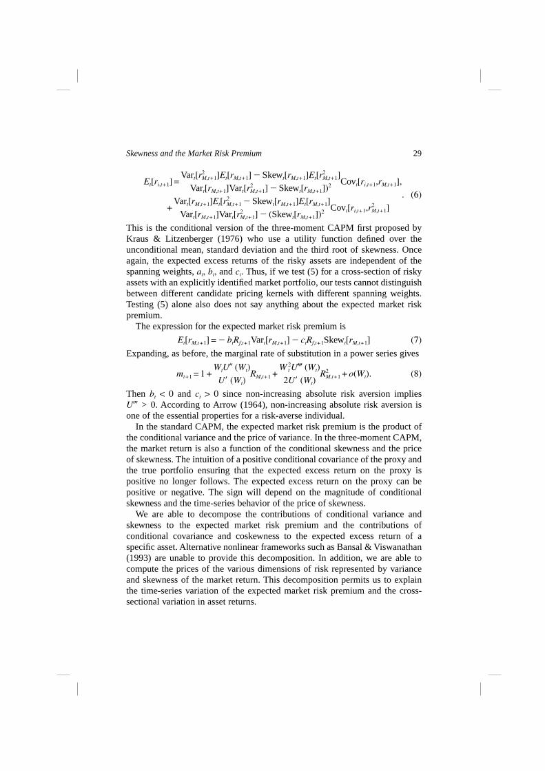
This is the conditional version of the three-moment CAPM first proposed byKraus & Litzenberger (1976) who use a utility function defined over theunconditional mean, standard deviation and the third root of skewness. Onceagain, the expected excess returns of the risky assets are independent of thespanning weights, at, bt, and ct. Thus, if we test (5) for a cross-section of riskyassets with an explicitly identified market portfolio, our tests cannot distinguishbetween different candidate pricing kernels with different spanning weights.Testing (5) alone also does not say anything about the expected market riskpremium.

The expression for the expected market risk premium is

Et[rM,t+1] = � btRf,t+1Vart[rM,t+1] � ctRf,t+1Skewt[rM,t+1] (7)

Expanding, as before, the marginal rate of substitution in a power series gives

mt+1 = 1 +WtU� (Wt)U� (Wt)

RM,t+1 +W 2

t U� (Wt)2U� (Wt)

R2M,t+1 + o(Wt). (8)

Then bt < 0 and ct > 0 since non-increasing absolute risk aversion impliesU� > 0. According to Arrow (1964), non-increasing absolute risk aversion isone of the essential properties for a risk-averse individual.

In the standard CAPM, the expected market risk premium is the product ofthe conditional variance and the price of variance. In the three-moment CAPM,the market return is also a function of the conditional skewness and the priceof skewness. The intuition of a positive conditional covariance of the proxy andthe true portfolio ensuring that the expected excess return on the proxy ispositive no longer follows. The expected excess return on the proxy can bepositive or negative. The sign will depend on the magnitude of conditionalskewness and the time-series behavior of the price of skewness.

We are able to decompose the contributions of conditional variance andskewness to the expected market risk premium and the contributions ofconditional covariance and coskewness to the expected excess return of aspecific asset. Alternative nonlinear frameworks such as Bansal & Viswanathan(1993) are unable to provide this decomposition. In addition, we are able tocompute the prices of the various dimensions of risk represented by varianceand skewness of the market return. This decomposition permits us to explainthe time-series variation of the expected market risk premium and the cross-sectional variation in asset returns.


3. ECONOMETRIC METHODOLOGY

The formulation of the asset pricing model is very general in that it permitstemporal variation in prices of variance and skewness risk as well as in theconditional moments themselves. The empirical estimation and tests of themodel confront us with two problems. First, we need to distinguish between thetime-varying prices of risk and the time-varying conditional moments. Second,we would like to avoid distributional assumptions about the conditionalmoments that do not come from the theory and may in fact conflict with it.Indeed, research has shown that the relation found between the conditionalmarket risk premium and conditional variance may be largely a function of thespecification chosen for the conditional moments. For example, Glosten,Jagannathan & Runkle (1993) report that using an asymmetric GARCH-Mspecification for conditional variance results in a positive relation betweenconditional risk premium and conditional variance whereas a regular GARCH-M yields a negative relation. We first document time-variation in theconditional moments using an explicitly chosen functional form for theconditional expectations. We also provide statistical tests. For example, we testwhether conditional skewness is evident in the data.

For the test of the model itself, we pursue two econometric formulations. Inthe first, we utilize the idea of Campbell (1987), Harvey (1989) and Dumas &Solnik (1995), where asset pricing restrictions can be tested without modellingthe conditional higher moments. We use Hansen’s (1982) generalized methodof moments for the tests. We begin by testing the restrictions on the time-seriesvariation in the expected market risk premium. We then add other assets anduse this method in cross-sectional analysis. Our technique allows us to recoverthe fitted prices of variance and skewness. To explain the temporal variation inthe expected market risk premium, we also need the corresponding highermoments. Therefore, we then estimate conditional skewness and variance in anon-parametric framework that imposes very few distributional assumptions.We combine the prices of risk with the conditional skewness and variance toget the expected market risk premium implied by the asset pricing model. Weevaluate the relation between the statistically fitted expected market riskpremium and theoretically implied expected market risk premium. We alsodetermine whether the addition of the conditional skewness and its time-varying price helps explain any of the negative ex ante risk premiums.

Ironically, the advantage of this first formulation (avoiding momentspecification) is also its disadvantage. Expected returns implied by asset pricingtheory can only be obtained by combining the prices of risk with fitted valuesfor the higher moments from an ancillary, separate estimation. This motivates


our second formulation. We jointly estimate the conditional mean, variance andskewness as well as the prices of variance and skewness in a conditionalmaximum likelihood framework. This requires us to choose explicit functionalforms for conditional variance and skewness. While heavily parameterized, thismodel allows us to directly test whether the addition of skewness helps explainthe negative risk premiums and avoids the two-step estimation problem.However, this estimation method is impractical for the large group of assetsincluded in cross-sectional analysis. Hence, this method is used only forunderstanding the time-series variation in the market risk premium.

3.1. Prices of variance and skewness risk

Campbell (1987), Harvey (1989) and Dumas & Solnik (1995) propose modelswhere restrictions can be tested without specifying the variance dynamics. Weextend this idea to skewness. Following Dumas & Solnik (1995), define theunexpected relative shock to the marginal rate of substitution:

ut+1 = �mt+1

E[mt+1 |�], (9)

where E[ut+1 | �t] = 0. Using ut+1 in (1) to substitute for mt+1 and using theconditionally riskfree rate of return to obtain the excess return:

E[rM,t+1(1 � ut+1) | �t] = 0

⇒E[rM,t+1 | �t] = E[RM,t+1ut+1 | �t] (10)

⇒E[rM,t+1 | �t] = Cov[RM,t+1,ut+1 | �t]

where the lower case rM,t+1 is the excess market return (market risk premium)and upper case RM,t+1 is the total market return. (9) and (10) impose restrictionson the conditional moments of the market risk premium. (10) should hold forexcess returns of all other risky assets as well. We assume that the unexpectedcomponent of mt+1 is spanned by a quadratic function of the market returnRM,t+1:

ut+1 = �0,t + �1,tRM,t+1 + �2,tR2M,t+1, (11)

where �1,t and �2,t are functions of period-t information set. Replacing ut+1 withthis function in (10) gives us:

E[rM,t+1|�t] = �1,tVar[RM,t+1|�t] + �2,tSkew[RM,t+1|�t]

=�0,t

(1 � �0,t)Rf,t+1 +

�1,t

(1 � �0,t)E[R2

M,t+1|�t] (12)

+�2,t

(1 � �0,t)E[R3

M,t+1|�t].


Comparing (12) to (7) tells us that �1,t and �2,t are the time-varying marketprices for variance and skewness risks, respectively. These two formulations forthe expected market risk premium are equivalent. They are respectively interms of the central and non-central conditional moments of the total marketreturn.

For assets other than the market portfolio, equation (12) becomes:

E[rj,t+1|�t] = �1,tCov[RM,t+1,Rj,t+1|�t] + �2,tCoskew[Rj,t+1,RM,t+1|�t] (13)

The coskewness between the market and the asset j is measured as thecovariance between Rj,t+1 and R2

M,t+1. This cross-sectional restriction impose thesame prices of risk for all the assets.

We assume that �i,ti = 0, 1, 2 are functions of Zt where Zt ��t. Zt areinstruments in the information set available to investors at time t. We use theformulation of the model with non-central moments of the total market returnand iterate the conditional expectations. Thus, the unconditional momentrestriction for the market return that follows (11) is

E[ut+1|Zt] = 0⇒E[(f0(Zt) + f1(Zt)RM,t+1

+ f2(Zt)R2M,t+1) � Zt] = 0,

where fi are the functional forms for the prices of risk, �i,t, since fi(Zt) = �i,t.Assuming that the fi are linear in Zt and using (10) give us the following two

restrictions

E[(��0Zt + ��1ZtRM,t+1 + ��2ZtR2M,t+1 � Zt] = 0.

E[(rM,t+1 � RM,t+1[��0Zt + ��1ZtRM,t+1 + ��2ZtR2M,t+1]) � Zt]. (14)

where �i are parameters in the prices of risk. These moment restrictions do notinclude any parameters for the conditional moments themselves.

The inequality restrictions on the prices of risk are �1,t ≥ 0 and �2,t ≤ 0.Non-negativity of mt+1 requires that ut+1 be less than 1. We test theunconditional moment restrictions using Hansen’s generalized method ofmoments (GMM). We estimate (14) with and without the inequality restrictionson the prices of risk. To impose the inequality restrictions, we use a quadraticspecification for f1 as square of a linear function, (��1Zt)

2, and f2 as � 1multiplied by a quadratic specification, i.e. � (��2Zt)

2. In all cases we use aheteroskedasticity consistent variance-covariance matrix with a Parzen kernel.The minimized GMM criterion function multiplied by the number ofobservations is distributed as a 2 with degrees of freedom equal to the numberof overidentifying restrictions which equals the number of orthogonalityconditions less the number of parameters. This is a specification test of themodel.


3.2. Non-parametric estimation of conditional moments

The second stage of our estimation involves the conditional moments. For eachof the returns, we need three moments. For the market portfolio proxy, we needthe conditional mean, variance and skewness. For the other asset returns, weneed the conditional mean, covariance with the market, and coskewness withthe market.

We first examine the market risk premium. We document that the conditionalmoments of the market risk premium vary over time using linear specifications.We then estimate the three conditional moments, mean, variance, and skewnesswithout imposing a functional form. We use non-parametric kernels to computethese conditional moments. The kernel method does not impose anydistributional assumptions on the market risk premium or the instruments. Themethod locally approximates the unknown underlying conditional density (ofthe market risk premium conditioned on the instruments) using a weighted sumof the market risk premia. The function chosen for the weighting scheme is thekernel or basis function. The expressions for the three moments using thekernel method are:

E[rM,t+1 | �t] = �T�1

j=1

rM,j+1Wt,j

Var[rM,t+1 | �t] = �T�1

j=1

(rM,j+1 � E[rM,j+1 | �j])2Wt,j (15)

Skew[rM,t+1 | �j] = �T�1

j=1

(rM,j+1 � E[rM,j+1 | �t])3Wt,j

where

Wt,j =K�Zt � Zj

h ��T�1

j=1

K�Zt � Zj

h �where K [] is the multivariate kernel function and h is the bandwidth, differentfor each conditional moment. The bandwidth determines the number of


observations that get a non-negligible weight. We use the multivariate Gaussiankernel function with bandwidth chosen to be asymptotically optimal for a meansquared error criterion. Thus, the conditional mean of the market risk premiumis formed as the weighted sum of all the market risk premia with the bandwidthdetermining which observations have non-negligible weights.

For conditional variance and skewness, we augment the instrument set, Zt, toinclude �2

t and �2t�1 for variance and �3

t and �3t�1 for skewness where �t is the

residual from the conditional mean estimation. Thus, for conditional varianceand skewness, our specification is in the spirit of a non-parametric ARCH(2)specification.

3.3. Conditional maximum likelihood estimation

As an alternative to the two-stage methodology, we use conditional maximumlikelihood estimation. Here, we assume explicit functional forms for the pricesof risk and the dynamics of the conditional moment evolutions. Then weimpose the restrictions on the moments implied by the theory and estimate theparameters in a conditional maximum likelihood framework. This methodallows us to avoid the problems of multistage estimation. There are moreparameters to estimate in the likelihood approach. However, when the uniqueelements of the weighting matrix are considered, the number of parameters toestimate in the GMM approach is in fact greater. This approach is feasible onlyfor the market risk premium.

The asset pricing model implies

rM,t+1 = �1,tVar[RM,t+1|�t] + �2,tSkew[RM,t+1|�t] + �t+1 (16)

To estimate the higher-order moments in (16), we assume that the expectedmarket risk premium is linear in the instrumental variables. Conditionalvariance needs to be strictly positive. To ensure the positivity, we compute theconditional standard deviation using the absolute residuals. For conditionalstandard deviations, we impose a GARCH(2,2) specification with instruments.The advantage of the GARCH specification is that it allows dependence on pastconditional variances. For skewness (which in our definition is not normalizedby the standard deviation), we also choose a GARCH(2,2) specification withinstruments. However, we do not impose any restrictions on the signs of theparameters. We assume the prices of variance and skewness risk are linear inthe instruments. Define ht+1 = Vart[rM,t+1] and st+1 = Skewt[rM,t+1] Thus:


�ht+1 = �0 + �2

i=1

�i|�t+1� i| + �2

i=1

i�ht+1� i + ��Zt

st+1 = �0 + �2

i=1

�i�3t+1� i + �2

i=1

�ist+1� i + ��Zt (17)

�1,t = ��1Zt

�2,t = ��2Zt

Assuming that the errors, �t+1, have a conditional t distribution we can write thesample log-likelihood function conditional on the first m observations as:

�T

t=1

ln f(�t+1|Zt, �) = T ln ��[� + 1)/2]

�1/2�[�/2](� � 2)�1/2��

1

2�T

t=1

ln(ht+1)

� [(� + 1)/2]�T

t=1

ln�1 +�2

t+1

ht(� � 2)� (18)

where � is the gamma function and � is the degrees of freedom of the tdistribution. The choice of t distribution is motivated by the evidence that evenafter assuming a GARCH specification for conditional variance, the distribu-tion of the residuals displays thick tails.

We also need to estimate the initial conditional variances and skewnesses, h1,h2, s1, and s2. Thus, the parameters to estimate are:

� = [�� 1�2�h1h2s1s2]�

The parameters are obtained by maximizing the sample log-likelihoodfunction.

We estimate the model with the inequality constraints (positive price ofvariance risk and negative price of skewness risk) as well as without theconstraints. As in the GMM-based methodology, to impose positivity on theprice of variance risk, we use the square of the linear function, (��1Zt)

2. Toensure negativity of the price of skewness risk, we use � 1 multiplied by thesquare of the linear function, –(��2Zt)

2.To test whether skewness enters the asset pricing model, we also estimate the

likelihood function (19) without skewness. This formulation of the model isequivalent to the standard CAPM. Twice the difference of the two sample log-likelihoods (with and without skewness) is approximately distributed as a 2(q)


where q is the number of parameters to estimate in the price of skewness riskand conditional skewness.

3.4. Data and Summary Statistics

We use several different data sets. For understanding the time-series behaviorof the market risk premium, we analyze three data sets. The first is studied byBoudoukh, Richardson & Smith (1993). These annual data include thehistorical U.S. stock market premium from 1802–1990. Second, we use themonthly U.S. data analyzed in Harvey (1989). This data set is from September1941 to December 1987 which we then update to September 1991. Finally, weexamine the data presented in Harvey (1991) and updated by Ostdiek (1994).These data measure world stock market returns at a monthly frequency from1970–1992.

The Boudoukh, Richardson & Smith (1993) annual data derives from themarket returns presented in Siegel (1990). Three instrumental variables areconstructed: the lagged short-term interest rate, the lagged dividend yield, andthe lagged slope of the term structure (as measured by the difference betweenlong and short-term interest rates).

In the Harvey (1989) data, the market portfolio return is the value-weightedNYSE index return from CRSP files. The instruments include: the laggedreturn on the equally-weighted NYSE index, the lagged yield spread betweenMoody’s Aaa and Baa rated bonds, the lagged excess return on a three monthTreasury bill, and the lagged excess U.S. dividend yield.

For the world data, the market return is Morgan Stanley Capital Internationalworld index. The instruments are: lagged world excess return, the lagged yieldspread between Moody’s Aaa and Baa rated bonds, the lagged excess return ona three month U.S. Treasury bill, and the lagged U.S. dividend yield.

Table 1 presents the summary statistics for the three proxies for the marketrisk premium. The results show, that for both the U.S. and MSCI worldportfolios, the ex-post market risk premium has been negative much more oftenthan the statistically fitted market risk premium. Using the a model that is linearin the instrumental variables, 3.2%, 25.8% and 32.7% of the statistically fittedmarket risk premia are negative for the U.S. annual, U.S. monthly and worldmonthly returns respectively. The R2s measuring predictability of the marketrisk premia are 6.3% for the annual U.S. data, 8.1% for the monthly U.S. and9.8% for the world. Using the cross-validated adaptive kernel this measure ofpredictability increases to 11.5% for the monthly U.S. and 12.4% for the world.However, for the annual series, the cross-validated adaptive kernel shows onlya trace amount of predictability. With the non-parametric measure, the


Table 1. A. Summary Statistics for the Market Risk Premia

Summary statistics are provided for the market risk premium for the US and MSCI world portfolios. The mean and standard deviation are for

annualized monthly returns. The skewness reported is the third central moment normalized by standard deviation cubed, E[�3

i,t]

�E[�2i,t

3

Mean Standard deviation Skewness Autocorrelation

U.S. 1941.09–1993.12 8.37 14.52 –0.40 0.08World 1970.02 – 1992.12 5.10 14.82 –0.34 0.11

B. Tests for Time-variation in conditional moments of market returnsGMM-based Wald tests for time-variation in the conditional mean, variance and skewness of the U.S. and MSCI world portfolio returns arepresented with a linear specification for for the time-varying moments:

E[rM,t+1|�t] = �0 + �4

i=1�iZit

E[R2M,t+1|�t] = �0 + �4

i=1�iZit + �2

i=1�iR

2M,t+1� i

E[R3M,t+1|�t] = �0 + �4

i=1�iZit + �2

i=1�iR

3M,t+1� i

where Zi are the four instruments Baa-Aaa yield spread, market return, excess holding period return for 3 month Treasury bill, and riskfree rate,RM is the market return and rM is the market risk premium. The variance and skewness are defined as the non-central moments of the total return.The statistics reported are the 2-values and the numbers in parentheses are significances or the probability of observing a larger 2-statistic underthe null hypothesis of no time-variation. The R2 is presented for the risk premium.

Market Risk Premium Variance SkewnessR2 2 p-value 2 p-value 2 p-value

U.S. 1941.09–1987.12 8.1% 32.87 (0.000) 47.17 (0.000) 23.52 (0.000)1941.09–1970.01 3.2% 9.47 (0.050) 21.90 (0.000) 10.27 (0.114)1970.01–1987.12 14.9% 41.74 (0.000) 23.88 (0.000) 32.89 (0.000)

World 1970.02–1992.12 9.8% 30.55 (0.000) 12.74 (0.047) 17.64 (0.007)1970.02–1979.12 15.6% 18.08 (0.001) 12.38 (0.054) 28.64 (0.000)1979.12–1992.12 7.2% 16.07 (0.003) 15.90 (0.014) 15.12 (0.019) 37

Skewness and the M

arket Risk P

remium

proportion of the statistically fitted market risk premia that is negative declines.Nevertheless, 10.3% of the U.S. and 21.1% of the world statistically fittedmonthly market risk premia are still negative. This suggests that a potentiallymisspecified linear specification can not be blamed for the negativity ofexpected market risk premia.

For both of the monthly U.S. and world portfolios, the unconditionalskewness is negative over the sample period. In contrast, the annual market riskpremium displays positive unconditional skewness over the period 1803–1990.However, consistent with the monthly data, in the subperiod 1941–1990, theannual U.S. market risk premium has negative skewness.

Figure 1 presents the fitted market risk premiums from both the OLS andnon-parametric models. Generally, the OLS and non-parametric fitted valueslook similar with a correlation between the two of 90% for the world portfolioand 84% for the U.S. portfolio. For the non-parametric analysis, we alsopresent two standard error confidence bands for the fitted values. For themonthly U.S. and world returns, the standard error bands confirm that a numberof the fitted values are negative. However, the standard error bands on theannual data are very large implying that there is little or no predictability in thereturns given these instruments. This may be a result of the early data beingapproximated, poor quality of the instruments or a fundamental lack ofpredictability. Nevertheless, it does not make much sense to proceed with amodel that attempts to explain the negative ex ante market risk premia withsuch large standard error bands. As a result, the rest of the paper concentrateson the evidence using monthly U.S. and world equity market returns. Previousstudies documenting negativity of the expected market risk premia have largelyused an explicit linear specification for the conditional mean. Hence, in the restof the paper we use the the OLS-based mean as our statistical fitted market riskpremium.

4. RESULTS: MARKET RISK PREMIUM

4.1. Prices of risk and conditional moments: GMM results

The asset pricing model suggests that the variation in conditional market riskpremium can be explained by variation in the prices of risk and the conditionalvariance and skewness with the conditional skewness potentially accountingfor the negative market risk premia. Thus, documenting the variation in theconditional moments needs to be the first step. We propose the following testsfor the variation of the conditional moments:


Fig. 1.


E[rM,t+1|�t] = �0 + �N

i=1

�iZit

E[R2M,t+1|�t] = �0 + �4

i=1

�iZit + �2

i=1

�iR2M,t+1� i (19)

E[R3M,t+1|�t] = �0 + �4

i=1

�iZit + �2

i=1

�iR3M,t+1� i

where as before the lower case represents the market risk premium (marketreturn in excess of the riskfree rate of return) and the upper case is the totalmarket return. We separately estimate each conditional moment in (19) usinggeneralized methods of moments and present Wald tests of their time-variation.The results are shown in panel B of Table I. For both U.S. and world portfolios,the tests reject the null hypotheses that the market risk premium, variance andskewness are constant over time. When we consider subperiods for the U.S.portfolio, variabilities of both conditional skewness and conditional market riskpremium have become more significant after 1970. For the world portfolio,skewness appears to be more significant than variance over the entire sample(which is from 1970) as well as in subperiods.

Table 2 presents tests of the model in (14) using generalized method ofmoments. For each of the data sets, we have 18 orthogonality conditions and 15parameters which produce 3 overidentifying restrictions. With 171 uniqueelements in the weighting matrix, the saturation ratio is 2.98 for the U.S. and1.48 for the world. Under the null hypothesis, that the model is correctlyspecified, the objective function multiplied by the number of observationsshould be distributed as a 2 with 3 degrees of freedom. For the U.S. portfoliowithout constraints on prices of risk, the objective function of the model has asuspiciously low value of 1.29 (p-value 0.73). For the constrained model, withthe price of variance risk constrained to be positive and the price of skewnessrisk constrained to be negative, the objective function has a value of 1.46 (p-value 0.69). Therefore, the null hypothesis cannot be rejected in either case at5% significance level. For the world portfolio, the unconstrained model with a2 statistic of 0.44 produces a p-value of 0.93. The constrained model has alarger 2 statistic of 5.35 resulting in a p-value of 0.15. Thus, we do not rejectthe null hypothesis for the world portfolio either. In all the cases, our Wald testson time-varying conditional skewness shows it to be significant.

As a diagnostic of the model, we also estimate a specification consistent withthe standard CAPM, i.e. (14) with the price of variance risk alone. For both the


Table 2. GMM-based Asset Pricing Model Tests on Market Risk Premium Without Parameterizing Variance& Skewness

The hypothesis that variance and skewness risk jointly explain the risk premium is tested by estimating:

E[��0Zt + ��1ZtRM,t+1 + ��2ZtR2M,t+1 � Zt] = 0.

E[[rM,t+1 � RM,t+1(��0Zt + ��1ZtRM,t+1 + ��2ZtR2M,t+1)] � Zt] = 0.

using generalized method of moments where rM is the market risk premium, RM is the total market return and Z are the instruments. For both theU.S. and World portfolios 18 orthogonality conditions and 15 parameters produce 3 overidentifying restrictions. The overidentifying 2 statistictests these restrictions. In addition, the skewness 2 statistic tests the significance of time-varying skewness by using a Wald test statistic. p-value,reported in parentheses, is the significance level at which the null hypothesis will be rejected. The CAPM 2 is for the test of overidentifyingrestrictions implied by the CAPM. u represents the average estimated relative shock to the marginal rate of substitution using both variance andskewness in the u-specification.

A. Unconstrained

Overidentifying 2 2 for Skewness = 0 u �(u) CAPM 2

U.S. 1.29 48.27 0.000 0.389 7.46(0.732) (0.000) (0.488)

World 0.44 20.17 0.422 3.518 0.76(0.932) (0.091) (0.999)

B. Constrained

Overidentifying 2 2 for Skewness = 0 u �(u) CAPM 2

U.S. 1.46 40.07 13.390 64.365 6.01(0.692) (0.000) (0.646)

World 5.23 22.99 0.201 0.422 10.34(0.156) (0.042) (0.242) 41

Skewness and the M

arket Risk P

remium

portfolios, the 2 for the overidentifying restrictions with variance risk alonehas a substantially larger value than the 2 for overidentifying restrictions withboth skewness and variance. These results, in Table II, confirm the importanceof incorporating skewness in the asset pricing model.

Another diagnostic is provided by the estimates of ut+1, the relative shock (orforecast error) to the marginal rate of substitution. For a proper, i.e. strictlypositive, marginal rate of substitution, ut+1 should be less than 1. Thus,estimates of ut+1 can gauge the economic reasonableness of difierent marketproxies used for the marginal rates of substitution. For the U.S. portfoliowithout constraints on the prices of risk, the average estimated shock is verysmall. Imposition of the constraints causes the estimated shocks to often exceed1. For the world portfolio, the average estimated shock is quite small with andwithout constraints. The constraints actually reduce the magnitude andvariability of estimated shocks. Thus, constraints on prices of risk appearreasonable for the world portfolio but untenable for the U.S. portfolio in lightof the unreasonably large estimates for the shocks to the marginal rate ofsubstitution. So constrained estimation for the U.S. portfolio is not that useful.

Estimation of the model in (14) also yields the market prices of variance andskewness risk, �1,t and �2,t respectively. We test whether those prices of risk areconstant over time with a likelihood ratio statistic. The statistic isT(gT(�R) � gT(�F)) where gT(�)F and gT(�)R are respectively the GMM objectivefunctions for the full and nested models. The nested model is estimated withthe same weighting matrix as the full model. For both the U.S. and worldportfolios, the tests presented in Table 3 reject the null hypothesis that theprices of variance and skewness risk are constant over time.

The price of variance risk is the market risk premium economic agentsdemand for an increase in conditional variance. Similarly, the price of skewnessrisk is the risk premium economic agents are willing to give up for an increasein conditional skewness. We examine how the prices of risk from the modelbehave in relation to the statistically fitted market risk premium. For theconstrained model using the U.S. portfolio, the statistically fitted market riskpremium has a correlation of 0.62 with price of variance risk and a correlationof –0.37 with the price of skewness risk. Thus, when expected market riskpremium increases, price of variance risk rises but the price of skewness riskbecomes more negative. For the constrained model using the world portfolio,correlation of the statistically fitted market risk premium with the prices ofvariance and skewness risks are 0.83 and –0.08 respectively. For both theportfolios, imposition of constraints required by theory reduce the variability ofthe prices of risk. This effect is particularly pronounced for the worldportfolio.


Table 3. Behavior of GMM-based Market Prices of Risk Without Parameterizing Variance & Skewness

The prices of variance and skewness risk are computed for the U. S. and MSCI world portfolios according to (16) using GMM. The standarddeviation shown is the variation of the estimated price of risk over time. For the constrained case, the price of variance risk is restricted to bepositive and the price of skewness risk is restricted to be negative. The unconstrained case does not impose any restrictions on the sign of theprices. The mean and standard deviation are multiplied by 103. To test time-variation in the prices a likelihood ratio test is used where the nestedmodel forces the prices of variance and skewness to be constants. The numbers in the parentheses report the probability of a larger 2 under thenull hypothesis of no time-variation. The degrees of freedom for the test are 8 for both the portfolios.

A. Unconstrained

Time-varying price Mean Standard deviation Negative % 2 for �i,t = �i

U.S. �0,t 0.35 8.32Monthly �i,t(Price of Variance Risk) 4.01 7.23 27.6% 21.491941.09–1987.12 �2,t(Price of Skewness Risk) 50.60 108.05 27.2% (0.005)

World �0,t –0.11 1.20Monthly �1,t(Price of Variance Risk) 38.75 66.35 22.7% 23.201970.02–1992.12 �2,t(Price of Skewness Risk) 188.07 190.96 9.5% (0.003)

B. Unconstrained

Time-varying price Mean Standard deviation

U.S. �0,t 0.09 1.42Monthly �1,t(Price of Variance Risk) 5.88 7.441941.09–1987.12 �2,t(Price of Skewness Risk) –12.17 27.99

World �0,t 0.18 1.30Monthly �1,t(Price of Variance Risk) 5.20 7.451970.02–1992.12 �2,t(Price of Skewness Risk) –10.63 18.82 43

Skewness and the M

arket Risk P

remium

Next we estimate the conditional variance and skewness using the non-parametric kernel approach described in Section 3.2. We then combine theprices of risk and the conditional moments to obtain the expected market riskpremium implied by the asset pricing model. Figure 2 shows the impliedmarket risk premium and the statistically fitted market risk premium for theU.S. and the world portfolios. If the model is true and if we could ignoreestimation and measurement errors, then the implied expected market riskpremium should be identical to the statistically fitted market risk premium. Ofcourse, this intuition also assumes that the statistically fitted market riskpremium is the true conditional mean of the market risk premium. We can notrealistically expect these assumptions to hold. Nevertheless, the degree towhich the dotted line (implied expected market risk premium) approximatesthe solid line (statistically fitted expected market risk premium) heuristicallyindicates the relative success or failure of the asset pricing model in explainingthe variation of the expected market risk premium for the two portfolios.

We find that for both the portfolios, imposition of the constraints on theprices of risk implied by the asset pricing theory improves the degree of fitbetween the statistically fitted market risk premium and the implied expectedmarket risk premium. The correlation increases from 0.23 to 0.33 for the U.S.and from 0.20 to 0.41 for the world portfolio. For the world portfolio inparticular, the reduction of the large gyrations in the implied expected marketrisk premium because of the constraints is very noticeable in the panels C andD of Fig. 2. With the constraints imposed, the average annualized expectedmarket risk premium for U.S. implied by the asset pricing model is 9.8%compared to the average annualized statistically fitted market risk premium of8.4%. For the world portfolio, the comparable numbers are 8.4% versus 5.1%.Thus, the asset pricing model has some success in explaining the variation ofthe expected market risk premia. The success is greater for the world portfolio.To check if the differing sample periods are responsible for the difference inperformance, we compare the performance over the common period1970.04–1987.12. In this period, the correlation between statistically fittedexpected market risk premium and the theoretically implied expected marketrisk premium is 0.41 for the world and only 0.06 for the U.S. portfolio.

4.2. Prices of risk and conditional moments: Maximum likelihood results

The generalized method of moments methodology has two drawbacks. First,we are compelled to use a two-step estimation procedure. Initially, we computethe prices of risk without having to make assumptions about the conditionalmoment dynamics. But when we compute the conditional moments, we can not


Fig

.2.


impose the restrictions on them (the moments) implied by asset pricing theory.Second, the saturation ratios for the two portfolios are low. These drawbacksmotivate our alternative estimation method. We model the conditional mean ofthe market risk premium using a linear specification. Then, we estimate theprices of risk and the higher conditional moments simultaneously in aconditional maximum likelihood framework using the residuals from the mean.Thus, the prices of risk and the corresponding higher conditional moments areestimated under the restrictions that arise from the theory.

The maximum likelihood results are presented in Table 4. For each of theportfolios, there are 31 parameters to estimate. The estimated degrees offreedom for the t-distribution in all four cases are approximately 3. Thisconfirms the presence of thick tails in the residuals.

The average log-likelihood for each of the models summarizes its relativesuccess in capturing the variation in the expected market risk premium. Forboth the portfolios, the average likelihood declines when constraints areimposed on the prices of risk. However, the decline is relatively small for theworld portfolio. We also see that the average likelihood for the world portfoliois larger than for the U.S. portfolio, though the sample size is smaller for theworld. Thus, it appears that the asset pricing model incorporating skewness isa better description for the world portfolio than for the U.S. portfolio. Theseresults are consistent with what we found using GMM.

Similar to our diagnostics for the GMM methodology, we also estimate amodel with variance alone that is equivalent to the standard CAPM. Theresults, also presented in Table 4, show that conditional skewness is significantfor explaining the variation in the expected market risk premium for the U.S.and world portfolios. Those conclusions are not affected by the imposition ofpositivity constraints. We also see that with variance alone the averagelikelihood declines much more precipitously for the world than for the U.S.This again confirms the greater importance of conditional skewness for theworld portfolio.

The prices of risk along with estimated conditional variance and skewnessare summarized in Table 5. The U.S. portfolio displays substantially greateraverage skewness than the world portfolio. For the world portfolio, theimposition of constraints on the prices of risk reduces the variability of theconditional moments. The absolute magnitudes of the prices of risk aresubstantially less than those obtained from the GMM methodology. For theU.S. portfolio, the mean of the unconstrained price of variance risk is negativeand mean of the price of skewness risk is positive. However, for the worldportfolio, the average prices of risk for variance and skewness are respectively


Table 4. Asset Pricing Model Tests on Market Risk Premium Using Conditional Maximum Likelihood

The average estimated conditional maximum likelihood values are presented for the monthly U.S. and world portfolio returns. The Skewness &Variance model assumes that the expected market risk premium is explained by both conditional variance and skewness of market returns andhas 33 parameters. The Variance Alone model assumes that the expected market risk premium is explained by conditional variance of marketreturns alone and has 17 parameters. This model is nested in the Skewness & Variance model and the significance of skewness is tested by thelikelihood ratio statistic

2(�(�Skewness & Variance) � (�(�Variance)) ~ 215

The constrained models force the price of variance risk to be strictly positive and the price of skewness risk to be strictly negative.

Unconstrained Constrained

Variance Alone Skewness & Variance 2 for Skewness = 0 Variance Alone Skewness & Variance 2 for Skewness = 0

U.S. 1.64 1.79 173.90 1.58 1.72 156.78(0.000) (0.000)

World 1.56 1.92 198.14 1.55 1.92 202.56(0.000) (0.000)

47Skew

ness and the Market R

isk Prem

ium

Table 5. Behavior of Conditional Maximum Likelihood-based Market Prices of RiskThe prices of variance and skewness risk are computed for the U.S. and MSCI world portfolios according to (19) using conditional maximumlikelihood assuming that the errors have a conditional t distribution. The standard deviation shown is the variation of the prices of risk andmoments over time. For the constrained case, the price of variance risk is restricted to be positive and the price of skewness risk is restricted tobe negative. The unconstrained case does not impose any restrictions on the sign of the prices. The mean and standard deviation are multipliedby 103.

A. Unconstrained

Time-varying price Mean Standard deviation Negative %

Price of Variance –8.122 45.668 59.02%U.S. Variance 1.442 0.9261941.09–1987.12 Price of Skewness 3.550 3.121 12.82%

Skewness –2369.494 1215.883

Price of Variance 2235.900 774.140 0.00%World Variance 2.173 3.7921970.02–1992.12 Price of Skewness –0.629 33.413 54.91%

Skewness –91.007 210.920

B. Constrained

Time-varying price Mean Standard deviation Negative %

Price of Variance 3.351 7.302U.S. Variance 1.639 0.5201941.09–1987.12 Price of Skewness –0.012 0.023

Skewness –3225.457 7025.516Price of Variance 360.970 270.210

World Variance 13.755 4.2271970.02–1992.12 Price of Skewness –5.359 9.845

Skewness –145.150 64.559

48C

AM

PBE

LL

R. H

AR

VE

Y &

AK

HTA

R SID

DIQ

UE

positive and negative. Thus, even without constraints, prices of risk for theworld portfolio display the right signs.

Combining the prices of variance and skewness risk with conditionalvariance and skewness, we obtain expected market risk premium implied by themodel for the two market portfolios. Figure 3 plots the expected market riskpremium implied by the higher conditional moments (with constraints on theprices of risk) along with the statistically fitted market risk premium. The plotsshow that for the model incorporating skewness is a much better fit for theworld portfolio than for the U.S. portfolio. With constraints on the prices ofrisk, the annualized average implied expected market risk premium for the U.S.is only 1.0% versus average statistically fitted market risk premium of 8.4%.For the world the comparable numbers are 6.0% versus 5.1%. Thus, theconstraints lead to unreasonable estimates for the U.S. portfolio. The figuresalso show that the implied expected market risk premium appears toapproximate the statistically fitted risk premium for the world much better thanfor the U.S. In fact, with constraints on prices of risk, the correlation betweenthe two is 47% for the world and 0% for the U.S. This corroborates the resultsin Table 4 that the average likelihood for the world portfolio return is higherthan for the U.S. portfolio return. Thus, as we found in the GMM-basedmethodology, the asset pricing model is more successful in explaining thevariation of the expected market risk premium for the world portfolio. Asbefore, to check if the differing sample periods are responsible for thedifference in performance, we compare the performance over the commonperiod 1970.02–1987.12. Using the constrained prices of risk, the correlationbetween statistically fitted expected market risk premium and the theoreticallyimplied expected market risk premium over this period is 47% for the worldand 6% for the U.S. portfolio.

4.3. Can the negative ex ante market risk premium be explained

To understand whether the incidences of ex-ante negative market risk premiumcan be explained by skewness, we need to analyze the interactions of the pricesof risk and the conditional moments. We consider two sets of periods, (1) whenthe statistically fitted market risk premium is negative and (2) when thestatistically fitted market risk premium minus the expected market riskpremium implied by conditional variance is negative. These are the periods ofinterest to us given that we are challenging the model to explain negative exante market risk premia. We can not expect any model to explain all theseperiods. However, the relative success for different models and differentportfolios permits us to draw some conclusions. For these periods we compute


Fig

.3.


the expected market risk premium implied by conditional skewness for both theU.S. and world portfolios with the two econometric methodologies, GMM andconditional maximum likelihood.

Of the 554 months in the U.S. market portfolio sample, the statistically fittedmarket risk premium is negative 143 times (25.8% of the months). For theworld portfolio, we have 275 months of data, of which 89 months (32.1%)show negative statistically fitted market risk premiums. When we constrain theprices of risk in maximum likelihood estimation in accordance with the assetpricing theory, the market risk premium implied by skewness is negative for 71of the 143 negative months for U.S. and 87 of the 89 negative months for theworld. Using GMM methodology and constraints, these proportions are lessimpressive.

The difference between the statistically fitted market risk premium and theexpected market risk premium implied by conditional variance can be viewedas the part of the market risk premium attributable to skewness risk. Usingmaximum likelihood and constraints on prices of risk, the U.S. portfolio hasnegative difference between statistically fitted market risk premium andexpected market risk premium implied by variance for 143 months (25.8% ofthe entire 554 month sample). For the world, 128 months (46.6% of the 275month sample) show such negativity. For the world, the expected market riskpremium implied by skewness is negative for 125 or 99.2% of the 128 months.For the U.S. the comparable number is 71 or 49.6% months out of 143. UsingGMM, the performance of the asset pricing model in explaining the episodesof negativity is much less impressive. But again, the performance is better forthe world portfolio than the U.S. portfolio.

Thus, the results show that the hypothesis that conditional skewness explainsthe negativity of the expected market risk premium has greater validity for theworld portfolio than the U.S. portfolio. Furthermore, when we constrain theprices of risk in accordance with asset pricing theory, the model is moresuccessful. These results are consistent with our findings in the previoussections showing that skewness itself is much more important for the worldportfolio than the U.S. portfolio.

The dichotomy between the U.S. and world portfolios may be due to thedifferent periods over which the data is available. But this hypothesis isuntenable in light of the significantly poorer performance of the model withconditional skewness in explaining the time-series variation of the expectedmarket risk premium for the U.S. than for the world portfolio when data overthe same period are used. Thus, there could be a fundamental differencebetween the two portfolios. Our tests should hold true for a valid proxy for themarket portfolio. Given the degree of integration in international capital


Table 6. Explanation of Negative Expected Risk Premia

The results in explaining the negative expected risk premia are summarized. The mean is modeled linearly in the instruments. The price ofvariance risk, �1,t, and the price of skewness risk, �2,t are estimated as linear functions in both maximum likelihood and GMM. For maximumlikelihood variance and skewness are modeled as GARCH(2,2). For GMM, variance and skewness are estimated with non-parametric kernels.

Maximum likelihood GMMUS World US World

Number of observations 554 275 554 275Number of negative ex ante risk premia 143 89 143 89Et[rM,t+1] < 0 25.8% 32.1% 25.8% 32.1%�2,tSkew[rM,t+1] < 0 Unconstrained 39.2% 63.3% 64.4% 60.7%when Et[rM,t+1] < 0 Constrained 49.6% 98.9% 27.3% 33.7%Et[rM,t+1 � �1,tVar[rM,t+1] < 0 Unconstrained 25.8% 45.1% 34.3% 72.2%

Constrained 25.8% 46.6% 47.6% 50.9%�2,tSkew[rM,t+1] < 0 Unconstrained 39.2% 66.9% 59.3% 46.7%when Et[rM,t+1] � �1,tVar[rM,t+1] < 0 Constrained 49.7% 99.2% 34.4% 41.0%Et[rM,t+1] and Et[rM,t+1] � �1,tVar[rM,t+1] < 0 Unconstrained 25.8% 32.1% 18.0% 24.9%

Constrained 25.8% 32.1% 25.8% 32.1%�2,tSkew[rM,t+1] < 0 Unconstrained 39.2% 63.3% 60.6% 60.3%when Et[rM,t+1] and Et[rM,t+1] � �1,tVar[rM,t+1] < 0 Constrained 49.6% 98.9% 27.3% 33.7%

52C

AM

PBE

LL

R. H

AR

VE

Y &

AK

HTA

R SID

DIQ

UE

markets and increasingly unimpeded flow of capital across borders, the worldportfolio should be a better proxy for the market. The U.S. portfolio is only acomponent of the world portfolio.

4.4. Extensions

The model and results presented in this paper have two interesting extensions.For both U.S. and world portfolios, the unconditional skewness has beennegative over the periods considered. Since the price of skewness should benegative, the implied risk premium from skewness should be positive as well.Hence, the implied market risk premium from variance and skewness should behigher than from variance alone for a large number of the periods. This has thepotential of explaining the equity market risk premium puzzle – the fact thatunconditionally the equity market risk premium is higher than what one shouldexpect from variance alone. Finally, the model and results of this paper willalso have implications for asset allocation and portfolio analysis. Instead ofanalyzing asset returns in a conditional mean-variance framework, a richerconditional mean-variance-skewness framework may be employed.

5. CONCLUSIONS

Recent research has found evidence against the single factor asset pricingmodel. The evidence on the time-series properties of the market risk premiumseems to suggest that the expected market risk premium is significantlynegative in some states of the world. Cross-sectional tests of the single factorasset pricing model have shown that systematic risk as measured by thecovariance (or the beta) with the market does not explain all of the cross-sectional variation in expected excess returns. We provide a possibleexplanation for these departures from the single factor asset pricing model. Ourintuition is that if investors know that the asset returns have conditionalskewness at time t, excess asset returns should include a component attributableto conditional skewness. Our asset pricing model formalizes this intuition byincorporating conditional skewness. This model can explain much of the time-series variation in the expected market risk premium.

We estimate this model for the U.S. and world portfolios using twomethodologies. The first is a generalized method of moments methodology thatdoes not require moment specifications for the portfolio returns. The second isa conditional maximum likelihood methodology that fully specifies the time-varying prices of risk and the dynamics of the conditional moments. Our resultsshow that conditional skewness is important and, when combined with the time


varying price of skewness, explains some of the negative ex ante market riskpremiums. Skewness is more important for the world market risk premium.Thus, for a model that requires us to specify a market portfolio, the worldportfolio appears to be a better proxy for the market. Consistent with thisfinding, the asset pricing model with conditional skewness has greater successin explaining the negativity of the expected market risk premium for the worldportfolio.

NOTES

1. Kane (1977) shows that if the asset returns follow diffusion processes, then mean-variance criterion is adequate only if continuous rebalancing is permitted. Therefore,without continuous rebalancing the moments of the discrete returns should includeskewness as well.

2. Also see Ingersoll (1990, pp. 199–201) for an alternative derivation for theunconditional three-moment CAPM. Sears & Wei (1985) also derive the unconditionalmarket risk premium as the sum of the market prices of variance and skewnessmultiplied by the moments. Since the riskfree rate does not possess variance orskewness, we can use variance and skewness of either the total returns or excessreturns.

3. Non-increasing absolute risk aversion implies that its derivative should be lessthan or equal to 0. U� ≥ 0 is a necessary condition to satisfy this. Also see Scott &Horvath (1980) for a discussion of the preference of moments beyond variance.

4. As an alternative, we also estimated conditional variance and skewness using aGARCH(2,2) specification similar to the specifications used in the conditionalmaximum likelihood estimation and used in Harvey & Siddique (1999). We do notreport the results but they do not change substantively using these fitted moments.

5. Pagan & Hong (1989) use a non-parametric ARCH specification for computingconditional variance. Also see Pagan & Schwert (1990) and Harvey (1991).

6. The linearity of the expected market risk premium follows Gibbons & Ferson(1985) and Campbell (1987).

7. Our approach extends the generalized autoregressive conditional heteroskedas-ticity, GARCH, to include autoregressive conditional skewness, and autoregressiveconditional kurtosis. For additional details on this methodology see Harvey & Siddique(1995).

8. Boudoukh, Richardson & Smith (1993) also use lagged volatility for a part of thesample. But it is not available for the whole sample.

9. This reflects the crashes in the historical returns.10. Boudoukh, Richardson & Smith (1993) find that they can not reject negativity of

the expected market risk premia using the same data. Their results do not rely onpredictability and they do not explicitly compute the expected market risk premia.However, one of our objectives is to explain the negativity of the expected market riskpremia. For this purpose, we need to compute the expected market risk premia.

11. We have computed all of the results using the non-parametric risk premiumswhich are available on request.


12. Saturation ratio is the number of observations divided by the number ofparameters to estimate and the number of unique elements in the weighting matrix.

13. We have also analyzed the properties of the conditional moments such assmoothness as diagnostics for our estimation.

14. In an economy with single consumption good, the expected market risk premiumcan not be negative. For the existence of a negative expected market risk premium in asingle factor model, non-traded sector of the economy is important.

15. Results using GMM and unconstrained risk prices are not presented but areavailable.

REFERENCES

Andrews, D. W. K. (1991). Heteroscedasticity and autocorrelation consistent covariance matrixestimation. Econometrica, 59, 817–858.

Arrow, K. J. (1964). Aspects of the theory of risk-bearing. lectures. Helsinki, Finland.Bansal, R., & Viswanathan, S. (1993). No arbitrage and arbitrage pricing. Journal of Finance, 48,

1231–1262.Black, F. (1972). Capital market equilibrium with restricted borrowing. Journal of Business, 44,

444–455.Boudoukh, J., Richardson, M., & Smith, T. M. (1993). Is the ex ante risk premium always positive?

Journal of Financial Economics, 34, 387–408.Brennan, M. J. (1993), Agency and asset pricing, Unpublished manuscript. UCLA and London

Business School.Campbell, J. Y. (1987). Stock returns and the term structure. Journal of Financial Economics, 18,

373–400.Carhart, M. M., & Krail, R. J. (1993). Testing the conditional CAPM. Unpublished manuscript.

University of Chicago.Carhart, M. M., Krail, R. J., Stevens, R. I., & Welch, K. E. (1994). Testing the conditional CAPM.

Unpublished manuscript. University of Chicago.Chan, L., Hamao, Y., & Lakonishok, J. (1991). Fundamentals and stock returns in Japan. Journal

of Finance, 46, 1739–1764.Cochrane, J. (1993). Unpublished lecture notes, University of Chicago.Christie, A. A. (1982). The stochastic behavior of common stock variances: value, leverage, and

interest rate effects. Journal of Financial Economics, 23, 407–432.Dumas, B., & Solnik, B. (1995). The world price of foreign exchange risk. Journal of Finance, 50,

445–479.Fama, E. F., & French, K. R. (1989). Business conditions and expected returns on stocks and

bonds, Journal of Financial Economics, 59, 23–49.Fama, E., & French, K. (1992). The cross-section of expected stock returns. Journal of Finance,

59, 427–465.French, K., Schwert, W., & Stambaugh, R. (1995). Expected stock returns and volatility. Journal

of Financial Economics, 19, 3–29.Friend, I., & Westerfield, R. (1980). Co-skewness and capital asset pricing. Journal of Finance, 35,

897–914.Gibbons, M. R., & Ferson, W. E. (1985). Tests of asset pricing models with changing expectations

and an unobservable market portfolio. Journal of Financial Economics, 10, 3–27.


Glosten, L. R., Jagannathan, R., & Runkle, D. E. (1993). On the relation between expected valueand the volatility of the nominal excess return on stocks. Journal of Finance, 48,1779–1801.

Hansen, L. P. (1982). Large sample properties of generalized method of moments estimators.Econometrica, 50, 1029–1054.

Hansen, L. P., & Jagannathan, R. (1991). Implications of security market data for models ofdynamic economies. Journal of Political Economy, 99, 225–262.

Hansen, L. P., & Richard, S. F. (1987). The role of conditioning information in deducing testablerestrictions implied by dynamic asset pricing models. Econometrica, 55, 587–613.

Harrison, M., & Kreps, D. (1979). Martingales and arbitrage in multi-period securities markets.Journal of Economic Theory, 20, 381–408.

Harvey, C. R. (1989). Time-varying conditional covariances in tests of asset pricing models.Journal of Financial Economics, 24, 289–317.

Harvey, C. R. (1991). The world price of covariance risk. Journal of Finance, 46, 111–157.Harvey, C. R., & Siddique, A. (1999). Autoregressive conditional skewness. Journal of Financial

and Quantitative Analysis, 34, 465–487.Harvey, C. R., & Siddique, A. (2000). Conditional skewness in asset pricing tests. Journal of

Finance. forthcomingIngersoll J. E. Jr. (1990). Theory of financial decision making. Totowa, New Jersey.Kandel, S., & Stambaugh, R. F. (1995). Bayesian inference and portfolio efficiency. Review of

Financial Studies, 8, 1–53.Kane, A. (1977). Skewness preference and portfolio choice. Journal of Financial and Quantative

Analysis, 17, 15–25.Kraus, A., & Litzenberger, R. H. (1976). Skewness preference and the valuation of risk assets.

Journal of Finance, 31, 1085–1100.Lim, K-G. (1989). A new test of the three-moment capital asset pricing model. Journal of

Financial and Quantative Analysis, 24, 205–216.Lintner, J. (1965). The valuation of risk assets and the selection of risky investments in stock

portfolios and capital budgets. Review of Economics and Statistics, 47, 13–37.Nelson, D. B. (1991). Conditional heteroskedasticity in asset returns. Econometrica, 59,

347–370.Nummelin, K. (1994). Expected asset returns and financial risks. Dissertation. Swedish School of

Economics and Business Administration (Svenska Handelshögskolan), Helskinki, Fin-land.

Ostdiek, B. (1994). The world ex ante risk premium: an empirical investigation. Unpublishedmanuscipt. Fuqua School of Business, Duke University.

Pagan, A. R., & Hong, Y. S. (1991). Non-parametric estimation and the risk premium. In: Non-parametric and semiparametric methods in econometrics and statistics, (51–75).Cambridge University Press, Cambridge.

Pagan, A. R., & Schwert, G. W. (1990). Alternative models for conditional stock volatility. Journalof Econometrics, 45, 267–290.

Roll, R., & Ross, R. (1994). On the cross-sectional relaion between expected returns and betas.Journal of Finance, 49, 101–121.

Roll, R. (1977). A critique of the asset pricing theory’s tests, Part I: On past and potentialtestability of theory. Journal of Financial Economics, 4, 129–176.

Ross, R. (1977). The capital asset pricing model (CAPM), short-sale restrictions and relatedissues. Journal of Finance, 32, 177–183.


Scott, R. C., & Horvath, P. A. (1980). On the direction of preference for moments of higher orderthan the variance. Journal of Finance, 35, 915–919.

Sears, R. S., & Wei, K. C. J. (1985). Asset pricing, higher moments, and the market risk premium:a note. Journal of Finance, 40, 1251–1253.

Sharpe, W. F. (1964). Capital asset prices: a theory of market equilibrium under conditions of risk.Journal of Finance, 19, 425–442.


TIME-VARYING CONDITIONAL SKEWNESS AND … CONDITIONAL SKEWNESS AND THE MARKET RISK ... present time-series evidence that the expected market risk premium is, ... As shown in Harvey

Documents