Time-Varying Across-Shelf Ekman Transport and Vertical Eddy Viscosity on the Inner Shelf ANTHONY R. KIRINCICH AND JOHN A. BARTH College of Oceanic and Atmospheric Sciences, Oregon State University, Corvallis, Oregon (Manuscript received 21 December 2007, in final form 6 August 2008) ABSTRACT The event-scale variability of across-shelf transport was investigated using observations made in 15 m of water on the central Oregon inner shelf. In a study area with intermittently upwelling-favorable winds and significant density stratification, hydrographic and velocity observations show rapid across-shelf movement of water masses over event time scales of 2–7 days. To understand the time variability of across-shelf exchange, an inverse calculation was used to estimate eddy viscosity and the vertical turbulent diffusion of momentum from velocity profiles and wind forcing. Depth-averaged eddy viscosity varied over a large dynamic range, but averaged 1.3 3 10 23 m 2 s 21 during upwelling winds and 2.1 3 10 23 m 2 s 21 during downwelling winds. The fraction of full Ekman transport present in the surface layer, a measure of the efficiency of across-shelf exchange at this water depth, was a strong function of eddy viscosity and wind forcing, but not stratification. Transport fractions ranged from 60%, during times of weak or variable wind forcing and low eddy viscosity, to 10%–20%, during times of strong downwelling and high eddy viscosity. The difference in eddy viscosities between upwelling and downwelling led to varying across-shelf exchange efficiencies and, potentially, increased net upwelling over time. These results quantify the variability of across-shelf transport efficiency and have significant implications for ecological processes (e.g., larval transport) in the inner shelf. 1. Introduction The mechanisms of across-shelf transport of water masses (and therefore nutrients, pollutants, phytoplankton, and planktonic larvae) in the inner shelf on wind-driven shelves are of significant scientific and public interest, controlling access between the stratified coastal ocean and the well-mixed surf zone. Recent studies (Lentz 2001; Kirincich et al. 2005) have reported that the ex- change driven by the alongshore wind decreases in re- lation to the total Ekman transport as the coast is approached, from 100% of full Ekman transport in water depths of 50 m to 25% in water depths of 15 m. This trend is based on mean results, averaged over sea- sonal (60–120 days) time periods. In contrast, wind-driven circulation varies over much shorter (2–7 days) time scales, and thus the factors that control this transport divergence may vary significantly. In this paper, we in- vestigate inner-shelf upwelling dynamics using obser- vations from the central Oregon coast in an attempt to quantify the variability of across-shelf exchange during the upwelling season. The central Oregon inner shelf is an ideal location to investigate wind-driven dynamics. The region is forced by upwelling-favorable winds with small offshore wind stress curl during the spring and summer months (Samelson et al. 2002; Kirincich et al. 2005). Throughout this time, intermittent downwelling wind bursts, occurring on periods of 5–20 days, lead to large variations in local circulation and hydrographic conditions. During the summer of 2004, the Partnership for Interdisciplinary Studies of Coastal Oceans (PISCO) program main- tained moorings at four along-shelf stations in 15 m of water on the Oregon inner shelf (Fig. 1). In a compan- ion work, Kirincich and Barth (2009) use these obser- vations to describe the temporal and spatial development of upwelling circulation. Summarizing their results, the three stations inshore of an offshore submarine bank— Seal Rock (SR), Yachats Beach (YB), and Strawberry Hill (SH)—were sheltered from the regional upwelling circulation yet still exposed to the regional wind forcing. In the lee of the bank (Barth et al. 2005), a smaller upwelling circulation formed near station SR and Corresponding author address: Anthony R. Kirincich, Woods Hole Oceanographic Institution, 266 Woods Hole Road, Woods Hole, MA 02543. E-mail: [email protected] 602 JOURNAL OF PHYSICAL OCEANOGRAPHY VOLUME 39 DOI: 10.1175/2008JPO3969.1 Ó 2009 American Meteorological Society

Welcome message from author
This document is posted to help you gain knowledge. Please leave a comment to let me know what you think about it! Share it to your friends and learn new things together.
Transcript
Time-Varying Across-Shelf Ekman Transport and Vertical Eddy Viscosity on theInner Shelf
ANTHONY R. KIRINCICH AND JOHN A. BARTH
College of Oceanic and Atmospheric Sciences, Oregon State University, Corvallis, Oregon
(Manuscript received 21 December 2007, in final form 6 August 2008)
ABSTRACT
The event-scale variability of across-shelf transport was investigated using observations made in 15 m of
water on the central Oregon inner shelf. In a study area with intermittently upwelling-favorable winds and
significant density stratification, hydrographic and velocity observations show rapid across-shelf movement of
water masses over event time scales of 2–7 days. To understand the time variability of across-shelf exchange,
an inverse calculation was used to estimate eddy viscosity and the vertical turbulent diffusion of momentum
from velocity profiles and wind forcing. Depth-averaged eddy viscosity varied over a large dynamic range,
but averaged 1.3 3 1023 m2 s21 during upwelling winds and 2.1 3 1023 m2 s21 during downwelling winds. The
fraction of full Ekman transport present in the surface layer, a measure of the efficiency of across-shelf
exchange at this water depth, was a strong function of eddy viscosity and wind forcing, but not stratification.
Transport fractions ranged from 60%, during times of weak or variable wind forcing and low eddy viscosity,
to 10%–20%, during times of strong downwelling and high eddy viscosity. The difference in eddy viscosities
between upwelling and downwelling led to varying across-shelf exchange efficiencies and, potentially,
increased net upwelling over time. These results quantify the variability of across-shelf transport efficiency
and have significant implications for ecological processes (e.g., larval transport) in the inner shelf.
1. Introduction
The mechanisms of across-shelf transport of water
masses (and therefore nutrients, pollutants, phytoplankton,
and planktonic larvae) in the inner shelf on wind-driven
shelves are of significant scientific and public interest,
controlling access between the stratified coastal ocean
and the well-mixed surf zone. Recent studies (Lentz
2001; Kirincich et al. 2005) have reported that the ex-
change driven by the alongshore wind decreases in re-
lation to the total Ekman transport as the coast is
approached, from 100% of full Ekman transport in
water depths of 50 m to 25% in water depths of 15 m.
This trend is based on mean results, averaged over sea-
sonal (60–120 days) time periods. In contrast, wind-driven
circulation varies over much shorter (2–7 days) time
scales, and thus the factors that control this transport
divergence may vary significantly. In this paper, we in-
vestigate inner-shelf upwelling dynamics using obser-
vations from the central Oregon coast in an attempt to
quantify the variability of across-shelf exchange during
the upwelling season.
The central Oregon inner shelf is an ideal location to
investigate wind-driven dynamics. The region is forced by
upwelling-favorable winds with small offshore wind stress
curl during the spring and summer months (Samelson
et al. 2002; Kirincich et al. 2005). Throughout this time,
intermittent downwelling wind bursts, occurring on
periods of 5–20 days, lead to large variations in local
circulation and hydrographic conditions. During the
summer of 2004, the Partnership for Interdisciplinary
Studies of Coastal Oceans (PISCO) program main-
tained moorings at four along-shelf stations in 15 m of
water on the Oregon inner shelf (Fig. 1). In a compan-
ion work, Kirincich and Barth (2009) use these obser-
vations to describe the temporal and spatial development
of upwelling circulation. Summarizing their results, the
three stations inshore of an offshore submarine bank—
Seal Rock (SR), Yachats Beach (YB), and Strawberry
Hill (SH)—were sheltered from the regional upwelling
circulation yet still exposed to the regional wind forcing.
In the lee of the bank (Barth et al. 2005), a smaller
upwelling circulation formed near station SR and
Corresponding author address: Anthony R. Kirincich, Woods
Hole Oceanographic Institution, 266 Woods Hole Road, Woods
Hole, MA 02543.
E-mail: [email protected]
602 J O U R N A L O F P H Y S I C A L O C E A N O G R A P H Y VOLUME 39
DOI: 10.1175/2008JPO3969.1
� 2009 American Meteorological Society
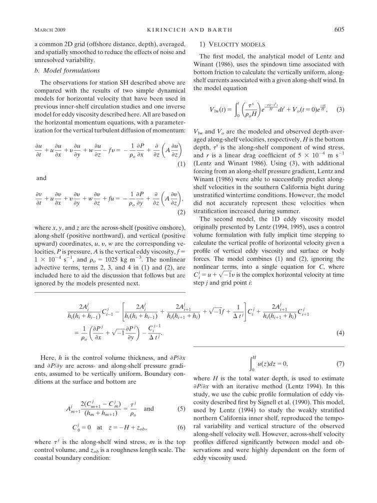
strengthened to the south. In this paper, we focus on
observations made by PISCO at the southernmost sta-
tion (SH) to describe the effects of intermittent forcing
on inner-shelf upwelling circulation.
We define the inner shelf as the region where across-
shelf Ekman transport is divergent and coastal up-
welling actively occurs. In this region, the thickness and
amount of overlap of the surface and bottom bound-
ary layers control the location of upwelling and the
local volume of across-shelf transport realized within
each boundary layer. Using Ekman dynamics (Ekman
1905), boundary layer thickness (d) is related to a ver-
tical eddy viscosity (A) through d 5 (2A/f )1/2, where f
is the Coriolis parameter. Here, the vertical turbulent
diffusion of momentum is parameterized as a function
of the vertical shear of the horizontal velocities and
eddy viscosity. By decreasing A, density stratification
should act to decrease the thickness of, and amount
of overlap between, the theoretical boundary layers at
a given water depth. Thus, variations in stratification
at these inner-shelf locations should have direct impli-
cations for across-shelf exchange of water masses in
the inner shelf and the ecological processes that depend
on it.
While the physical mechanisms controlling across-shelf
exchange are well studied in coastal regions dominated
by buoyant plume dynamics (Wiseman and Garvine
1995; Yankovsky et al. 2000; Garvine 2004), both ob-
servational and modeling studies of wind-driven inner-
shelf dynamics have had difficulties describing and fully
resolving across-shelf exchange variability. Wind-driven
across-shelf velocities in the inner shelf are difficult to
observe, being an order of magnitude smaller than wind-
driven along-shelf velocities, tidal motions, and wave or-
bital velocities. Thus, measurement errors or unresolved
spatial scales inhibit proper closure of the momentum
balances. If the coastal boundary and bathymetry are
locally straight and uniform, analytical models can cap-
ture the majority of the along-shelf variability of wind- or
pressure-driven inner-shelf systems during weakly strat-
ified conditions (Lentz and Winant 1986; Lentz 1994).
However, across-shelf currents and stratified conditions
are more difficult to properly represent, in part due to an
oversimplification of vertical diffusion of momentum in
these models.
Recently, two-dimensional (2D) numerical models
with higher-order turbulent closure schemes have been
used with some success to investigate inner-shelf circu-
lation during constant wind (Austin and Lentz 2002)
and realistic wind (Kuebel Cervantes et al. 2003) forc-
ing. In their parameterizations of the vertical turbulent
diffusion of momentum, eddy viscosity is a function of
the distance to the boundary, local stratification, in-
stantaneous velocity, and velocity shear (Mellor and
Yamada 1982). These estimates of eddy viscosity and
the vertical diffusion of momentum were critical to the
dynamical balances that Austin and Lentz (2002) and
Kuebel Cervantes et al. (2003) obtained. Both studies
noted a dynamical difference in vertical diffusion on the
inner shelf during upwelling and downwelling condi-
tions. Further, Austin and Lentz (2002) reported that
across-shelf transport decreased as stratification decreased
and the vertical diffusion of momentum increased. Thus,
with weaker stratification occurring during downwelling
conditions, across-shelf exchange at a given water depth
during downwelling was reduced relative to that seen
during upwelling.
Our analysis of the event-scale (2–7 days) upwelling
dynamics would also benefit from estimates of the vertical
turbulent diffusion of horizontal momentum, as it should
be the ultimate controller of boundary layer thickness,
FIG. 1. The central Oregon shelf with the 2004 PISCO stations
(dots) and the Newport C-MAN station (triangle) marked. The
bold line offshore of SH marks the transect line occupied during
the high-resolution ship-based surveys. Isobaths (thin black lines)
are marked in meters.
MARCH 2009 K I R I N C I C H A N D B A R T H 603
the amount of overlap, and the efficiency of across-shelf
Ekman transport. However, the observations necessary to
directly measure the turbulent fluxes are rarely made
in the inner shelf, especially over extended deployment
periods encompassing forcing events. Thus, we use a
novel approach to estimate this term by inverting the
one-dimensional (1D) model of Lentz (1994) to solve
for vertical eddy viscosity and vertical turbulent diffu-
sion given a known surface forcing and the observed
velocity profiles. The novelty of this approach is that an
optimization is used to estimate vertically uniform pres-
sure gradients and account for unknown sources (or
sinks) of momentum while keeping the form of vertical
diffusion intact. Using this estimated eddy viscosity, we
are able to explain the event-scale variability of across-
shelf circulation in the study area.
In this paper we describe the short-time-scale (2–7
days) variability of inner-shelf circulation, hydrography,
and forcing along the central Oregon coast during
summer and document the dependence of across-shelf
transport on an estimate of vertical turbulent diffusion.
We begin by describing the moored and shipboard ob-
servations of the study area, and detailing the numerical
model formulations used in our analysis (section 2).
Results consist of a detailed description of the event-
scale circulation variability, the estimated eddy viscosity,
depth-dependent momentum balances, and a quantifi-
cation of the time-dependent across-shelf exchange effi-
ciency (section 3). The influence of this variable effi-
ciency on inner-shelf circulation is discussed (section 4)
before we summarize our results (section 5).
2. Data and methods
a. Observations
Between 9 July and 7 September 2004 (yeardays 190
and 250), velocity profiles and hydrographic measure-
ments were collected at station SH by moored instru-
ments maintained by PISCO (Fig. 1). Data from a similar
deployment at station SR, located 27 km to the north,
are used to estimate along-shelf gradients of momentum
at SH. At each station a bottom-mounted, upward-
looking acoustic Doppler current profiler (ADCP) was
deployed adjacent to a mooring of temperature and
conductivity sensors. The ADCP, an RDI Workhorse
600-kHz unit, collected velocity profiles in 1-m incre-
ments from 2.5 m above the bottom to 1 m below the
surface and sampled pressure at the instrument depth
(14.5 m). The nearby mooring measured temperature
at 1, 4, 9, and 14 m below the surface with Onset Tidbit
or XTI loggers and temperature and conductivity
at 8 and 11 m using Sea-Bird 16 or 37 conductivity–
temperature (CT) recorders. Wind measurements col-
lected at National Oceanic and Atmospheric Adminis-
tration’s (NOAA) Coastal-Marine Automated Network
(C-MAN) station NWP03 are used for this analysis. Sta-
tion NWP03, located 30 km north of SH at Newport,
Oregon, has been previously found to be representative
of near-shore winds throughout the study area during
summer (Kirincich et al. 2005; Samelson et al. 2002).
From these observations, sampled every 2 to 10 min,
we derived hourly averaged time series of along-shelf
velocity, across-shelf surface transport, pressure anom-
aly, and density profiles using the steps outlined below.
The hourly averaged water velocities were rotated into
an along- and across-shelf coordinate system defined by
the depth-averaged principal axis of flow, found to be 78
(for SH) and 18 (for SR) east of true north. Time series
of across-shelf surface transport were computed from
velocity profiles, extrapolated to the surface and bottom
assuming a constant velocity (slab) extrapolation, by
subtracting the depth-averaged mean and integrating
the profiles from the surface to the first zero crossing,
following Kirincich et al. (2005). Pressure anomaly was
calculated by subtracting an estimate of the tidal vari-
ability, found using the T_TIDE software package
(Pawlowicz et al. 2002), and a mean pressure time se-
ries, calculated following Kirincich and Barth (2009).
Density was estimated throughout the water column
using the 8-m salinity measurement and each of the five
temperature locations, assuming a linear relationship
between temperature and salinity (m 5 8.48C psu21)
derived from nearby conductivity–temperature–depth
(CTD) casts. All time series were low-pass filtered using
a filter with a 40-h half-power period to isolate the
subtidal components. Correlations between time series
were tested for significance using the 95% confidence
interval for the level of significance and N*, the effective
degrees of freedom, following Chelton (1983).
In addition to the moored observations, a high-reso-
lution hydrographic and velocity survey of the area was
conducted from the research vessel (R/V) Elakha on
9–11 August (yeardays 222–224). Each day, at the same
phase of the tide, two to four consecutive 1-h transects
were made along an east–west line terminating onshore
at station SH (Fig. 1). Water depths along the transect
line ranged from 15 m onshore to 70 m offshore, 12 km
from the coast. Hydrographic measurements were ob-
tained using a Sea Sciences Acrobat, a small, undulating
towed body, carrying a Sea-Bird 25 Sealogger CTD.
Velocity estimates were made with a 300-kHz RDI
Workhorse Mariner ADCP mounted on the R/V Elakha.
Initial processing of these ship-based observations fol-
lows the methods described by Kirincich (2003). Density
and velocity fields for each transect were interpolated to
604 J O U R N A L O F P H Y S I C A L O C E A N O G R A P H Y VOLUME 39
a common 2D grid (offshore distance, depth), averaged,
and spatially smoothed to reduce the effects of noise and
unresolved variability.
b. Model formulations
The observations for station SH described above are
compared with the results of two simple dynamical
models for horizontal velocity that have been used in
previous inner-shelf circulation studies and one inverse
model for eddy viscosity described here. All are based on
the horizontal momentum equations, with a parameter-
ization for the vertical turbulent diffusion of momentum:
›u
›t1 u
›u
›x1 y
›u
›y1 w
›u
›z� f y 5 � 1
ro
›P
›x1
›
›zA
›u
›z
� �(1)
and
›v
›t1 u
›y
›x1 y
›y
›y1 w
›y
›z1 fu 5 � 1
ro
›P
›y1
›
›zA
›y
›z
� �,
(2)
where x, y, and z are the across-shelf (positive onshore),
along-shelf (positive northward), and vertical (positive
upward) coordinates, u, y, w are the corresponding ve-
locities, P is pressure, A is the vertical eddy viscosity, f 5
1 3 1024 s21, and ro 5 1025 kg m23. The nonlinear
advective terms, terms 2, 3, and 4 in (1) and (2), are
included here to aid the discussion that follows but are
ignored by the models presented next.
1) VELOCITY MODELS
The first model, the analytical model of Lentz and
Winant (1986), uses the spindown time associated with
bottom friction to calculate the vertically uniform, along-
shelf currents associated with a given along-shelf wind. In
the model equation
V lw(t) 5
ðt
0
t s
roH
� �e�r(t�t0 )
H dt01 Vo(t 5 0)e�rtH , (3)
Vlw and Vo are the modeled and observed depth-aver-
aged along-shelf velocities, respectively, H is the bottom
depth, ts is the along-shelf component of wind stress,
and r is a linear drag coefficient of 5 3 1024 m s21
(Lentz and Winant 1986). Using (3), with additional
forcing from an along-shelf pressure gradient, Lentz and
Winant (1986) were able to successfully predict along-
shelf velocities in the southern California bight during
unstratified wintertime conditions. However, the model
did not accurately represent these velocities when
stratification increased during summer.
The second model, the 1D eddy viscosity model
originally presented by Lentz (1994, 1995), uses a control
volume formulation with fully implicit time stepping to
calculate the vertical profile of horizontal velocity given a
profile of vertical eddy viscosity and surface or body
forces. The model combines (1) and (2), ignoring the
nonlinear terms, into a single equation for C, where
Cji 5 u 1
ffiffiffiffiffiffiffi�1p
y is the complex horizontal velocity at time
step j and grid point i:
Here, h is the control volume thickness, and ›P/›x
and ›P/›y are across- and along-shelf pressure gradi-
ents, assumed to be vertically uniform. Boundary con-
ditions at the surface and bottom are
Ajm11
2(Cj
m11� C j
m)
(hm 1 hm11)5
t j
ro
and (5)
Cj0
5 0 at z 5�H 1 zob, (6)
where t j is the along-shelf wind stress, m is the top
control volume, and zob is a roughness length scale. The
coastal boundary condition:
ðH
0
u(z)dz 5 0, (7)
where H is the total water depth, is used to estimate
›P/›x with an iterative method (Lentz 1994). In this
study, we use the cubic profile formulation of eddy vis-
cosity described first by Signell et al. (1990). This model,
used by Lentz (1994) to study the weakly stratified
northern California inner shelf, reproduced the tempo-
ral variability and vertical structure of the observed
along-shelf velocity well. However, across-shelf velocity
profiles differed significantly between model and ob-
servations and were highly dependent on the form of
eddy viscosity used.
2Aji
hi(hi 1 hi�1)C
ji�1�
2Aji
hi(hi 1 hi�1)1
2Aji11
hi(hi11 1 hi)1
ffiffiffiffiffiffiffi�1p
f 11
D t j
" #C
ji 1
2Aji11
hi(hi11 1 hi)C
ji11
51
ro
›P j
›x1
ffiffiffiffiffiffiffi�1p ›P j
›y
� ��
Cj�1
i
D t j. (4)
MARCH 2009 K I R I N C I C H A N D B A R T H 605
2) EDDY VISCOSITY MODEL
In the forward model described above, velocity pro-
files are estimated given the wind or pressure forcing
and an assumed vertical profile of eddy viscosity. Here,
we seek an inverse solution to (1) and (2) that estimates
the time-dependent vertical profile of eddy viscosity
given vertical profiles of horizontal velocity and wind
forcing. Reordering Eq. (4) to solve for eddy viscosity
(A) gives
�2(C
ji � C
ji�1
)
(hi 1 hi�1)A
ji 1
2(Cj
i11� C
ji )
(hi11 1 hi)A
ji11
5ffiffiffiffiffiffiffi�1p
fCj
i hi
1hi
ro
›P j
›x1
ffiffiffiffiffiffiffi�1p ›P j
›y
� �1
(Cj
i � Cj�1
i )
Dtjhi, (8)
a first-order ODE requiring knowledge of the horizon-
tal pressure gradients (›P/›x and ›P/›y), the horizontal
velocities, and one boundary condition. We use the
surface (wind) forcing (5) to obtain eddy viscosity at the
surface.
Of the three inputs to the inverse solution, the pressure
gradients are perhaps the most difficult to measure di-
rectly. Estimates of the barotropic across-shelf and along-
shelf pressure gradients at the PISCO stations were made
by Kirincich and Barth (2009), yielding a geostrophically
balanced pressure gradient in the across-shelf direction
and variable pressure gradient in the along-shelf direc-
tion (Figs. 5d,e). Additionally, a test of the thermal wind
balance, reported in section 3a found similarities be-
tween a vertically sheared Coriolis term and the across-
shelf density gradient offshore of SH during upwelling-
favorable winds. However, these pressure gradients were
not measured with sufficient accuracy to be used in (8)
(Kirincich and Barth 2009) and thus must be treated as
unknowns. To simplify the inverse formulation with
these additional unknowns, we assume the majority of
the depth-dependent Coriolis term at this shallow-water
depth is in an Ekman balance with vertical diffusion
rather than a geostrophic balance with a baroclinic
pressure gradient. Thus, the depth-dependent pressure
gradients should be much smaller than both the vertically
uniform pressure gradients and the vertical diffusion
terms, and they can be ignored. This assumption has been
used in previous models (Lentz and Winant 1986; Lentz
1994) and is tested in section 3c.
With these simplifications, given a pair of pressure
gradients, we can solve (8) for a vertical profile of eddy
viscosity using only the velocity profiles and wind stress
as input. However, if the velocity profiles are not fully
explained by the input forcing, the resulting eddy vis-
cosity will be incorrect and possibly complex. The imag-
inary part of such a result can be understood dynamically
considering the balance of momentum. A residual mo-
mentum term will exist if the vertical diffusion term,
with its magnitude and vertical structure driven by the
unknown eddy viscosity and the velocity shear, is un-
able to account for all of the remaining momentum. In
the inverse solution, this residual is packaged into an
imaginary part of the eddy viscosity, and thus has a
component in each momentum equation (denoted as Rx
and Ry). We assume that the bulk of this incorrect or
additional momentum is due to incorrect vertically
uniform pressure gradients. To optimize the solution,
(8) is solved for a matrix of along- and across-shelf
pressure gradient pairs, finding the pair that makes the
profile of A as positive as possible [as vertical diffusion
is a momentum sink (A . 0) not a source (A , 0)] and
minimize the depth-averaged absolute value of the re-
sidual momentum terms Rx and Ry.
The inverse solution is calculated independently for
each time step j, providing time series of the estimated
eddy viscosity (A; Fig. 5c), the vertically uniform along-
and across-shelf pressure gradients that optimize the
inverse solution for the criteria given above (hereafter
‘‘matched’’ pressure gradients; Figs. 5d,e), and the
depth-dependent residual momentum terms Rx and Ry.
The raw, hourly velocity profiles used in the calculation
were normalized by water depth, interpolated onto a
regularly spaced vertical grid, and low-pass filtered to
isolate the subtidal variability. The along-shelf compo-
nent of wind stress, also low-pass filtered, was used as
the surface boundary condition. The matched pressure
gradients are assumed to be composed of the vertically
uniform pressure gradient and the depth-averaged mean
of any other unrepresented term in the momentum
equations (e.g., nonlinear advection), while the residual
momentum term accounts for the depth-dependent part
of any unrepresented term.
Accuracy testing for the inverse solution was done
using the output of several numerical circulation models
as described by Kirincich (2007). Summarizing these
results, tests indicate that the inverse calculation was
unable to reasonably estimate eddy viscosity when the
vertical shear of the horizontal velocity was less than
5 3 1023 s21. Approximately 4.4% of the observations
from station SH fell below this threshold. Additionally,
the inverse did poorly when the true eddy viscosities
were less than 5 3 1025 m2 s21. Approximately 4.2% of
the estimated eddy viscosity values fell below this
threshold. (Instances of poor fit included in these
thresholds can also be seen in Fig. 5c as negative val-
ues or sharp spikes of A.) Above these levels, tests using
the numerical models imply that rms errors are 20%
of the mean eddy viscosity values for upwelling and
606 J O U R N A L O F P H Y S I C A L O C E A N O G R A P H Y VOLUME 39
downwelling if the inverse solution is well formulated. If
additional sources or sinks of momentum have been
neglected, potential errors increase with depth from
20% to 70% of the mean values, but approach the mean
values themselves in the bottom 2–3 m.
The inverse method described here does not account
for measurement errors of the velocity or wind data
while estimating vertical diffusion and eddy viscosity.
Thus, more complex variational estimation techniques
that do so (Yu and O’Brien 1991; Panchang and
Richardson 1993) could be adapted to solve for time-
dependent profiles of A. However, we proceed with the
basic model described above to understand how varia-
tions in vertical eddy viscosity over the time scales of
wind and pressure forcing events can effect across-shelf
circulation in the inner shelf. Based on the accuracy and
sensitivity of the method, the inverse calculation for-
mulated here was deemed adequate for this purpose.
c. Calculating momentum balances
The distribution of momentum in the inverse model
results can be packaged into four terms for each linear
horizontal momentum equation: the measured acceler-
ation, an ageostrophic pressure gradient formed by the
sum of the Coriolis and matched pressure gradient
terms, the vertical diffusion of momentum, and a re-
sidual momentum term (Figs. 7a–d, 8a–d). Vertical
profiles of vertical diffusion and residual momentum
were smoothed (using a three-point boxcar vertical fil-
ter) for presentation in Figs. 7 and 8. For comparison
with the residual term, estimates of across-shelf and
vertical advection, the second and fourth terms of (1)
and (2), are included (Figs. 7e,f, 8e,f). Across-shelf ad-
vection uses station SH velocities and an across-shelf
velocity gradient between the measurements at SH and
zero at the coastal boundary. Vertical advection was
computed by multiplying the vertical gradients of hor-
izontal velocities at station SH by an estimate of the
vertical velocity w. We assumed w had a parabolic ver-
tical structure that was zero at both boundaries and a
maximum at middepth, where it equaled the across-shelf
surface transport at station SH divided by the distance to
the outside of the surf zone (700 m). In both equations,
estimates of the along-shelf momentum flux, the third
term in (1) and (2), were an order of magnitude smaller
than all other terms and were neglected hereafter.
3. Results
a. Observed hydrographic variability
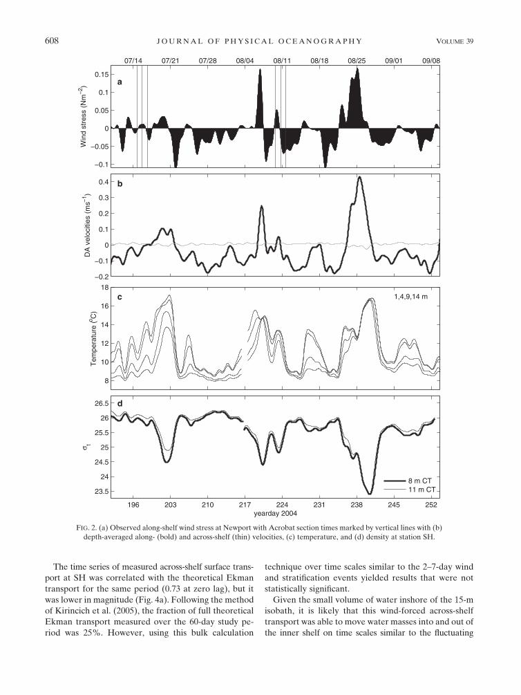
We begin with a description of conditions at station
SH during the later half of the 2004 upwelling season
(Fig. 2). In general, the study area was forced by
upwelling-favorable winds (t 5 20.05 N m22) that re-
sulted in southward velocities near 0.1 m s21 and dense
waters (st 5 25.5–26 kg m23) in the inner shelf. Periodic
wind reversals occurring near days 203, 220–224, and
236–242 (Fig. 2) caused reversals of along-shelf velocity
and reduced inner-shelf density. Water-column tem-
peratures ranged from 88 to 98C during strong or sus-
tained upwelling, and 148 to 168C during these current
reversals. Waters tend to be more stratified during pe-
riods of weaker winds (e.g., days 195–202 and 227–232),
weakly stratified during upwelling conditions (e.g., days
206–215 and 224–227), and nearly unstratified during
peak downwelling events (e.g., days 219 and 238–241)
(Fig. 2). This hydrographic variability implies that con-
ditions regularly transition between fully upwelled
(when the upwelling front intersects the surface offshore
of the mooring, leaving weakly stratified conditions in-
shore) and fully downwelled (similar conditions but for
a downwelling front) in response to the local wind
forcing.
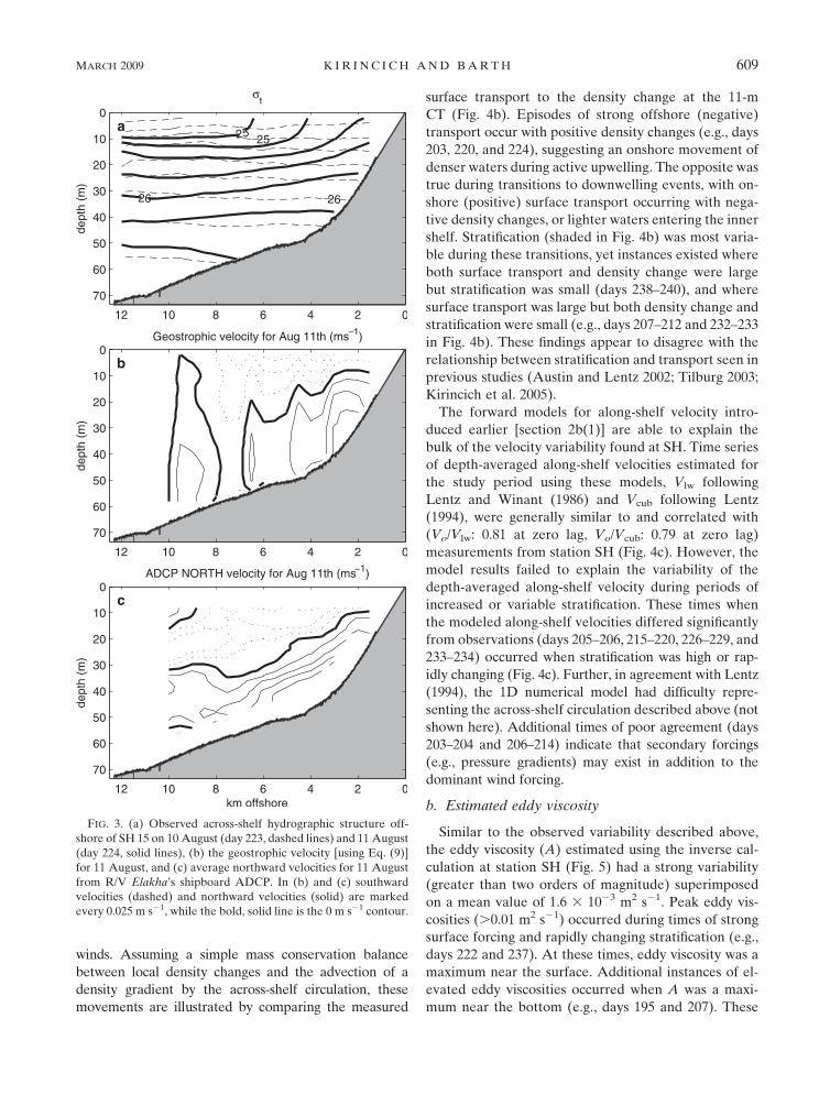
These rapid wind-driven fluctuations are further il-
lustrated by the across-shelf sections obtained on 10 and
11 August (yeardays 223 and 224) shown in Fig. 3. During
this period, winds transition from a short downwelling
event (day 222) to strengthening (day 223) and then
sustained (day 224) upwelling (Fig. 2a). The across-shelf
hydrographic sections (Fig. 3a) show isopycnals tran-
sitioning from nearly horizontal on day 223 (dashed
lines) to strongly upwelled on day 224 (solid lines). The
st 5 25 kg m23 isopycnal lies at a depth of 10 m inshore
of the 15-m isobath (1.5 km offshore) on day 223, but
intersects the surface near the 50-m isobath (6.5 km
offshore) one day later. Assuming along-shelf unifor-
mity, a water parcel at this interface would need an
average across-shelf velocity of 0.06 m s21 to attain this
displacement. Comparing the ship-based hydrography
and velocity surveys using the thermal wind equation,
›y
›z5
g
rof
›st
›x, (9)
where g 5 9.81 m s22 is the gravitational acceleration,
shows that the across-shelf density structure was nearly
geostrophically balanced by along-shelf velocities on
day 224 (Figs. 3b,c). Using the surface (z 5 0) as the
reference level and the ADCP-derived near-surface
velocity as the reference velocity, density-derived geo-
strophic velocities were similar to the ADCP-derived
velocities offshore of the 20-m isobath in vertical shear,
magnitude, and direction. The rms difference between
the two sections was 0.037 m s21 overall, but 0.025 m s21
within the area of the upwelled isopycnals.
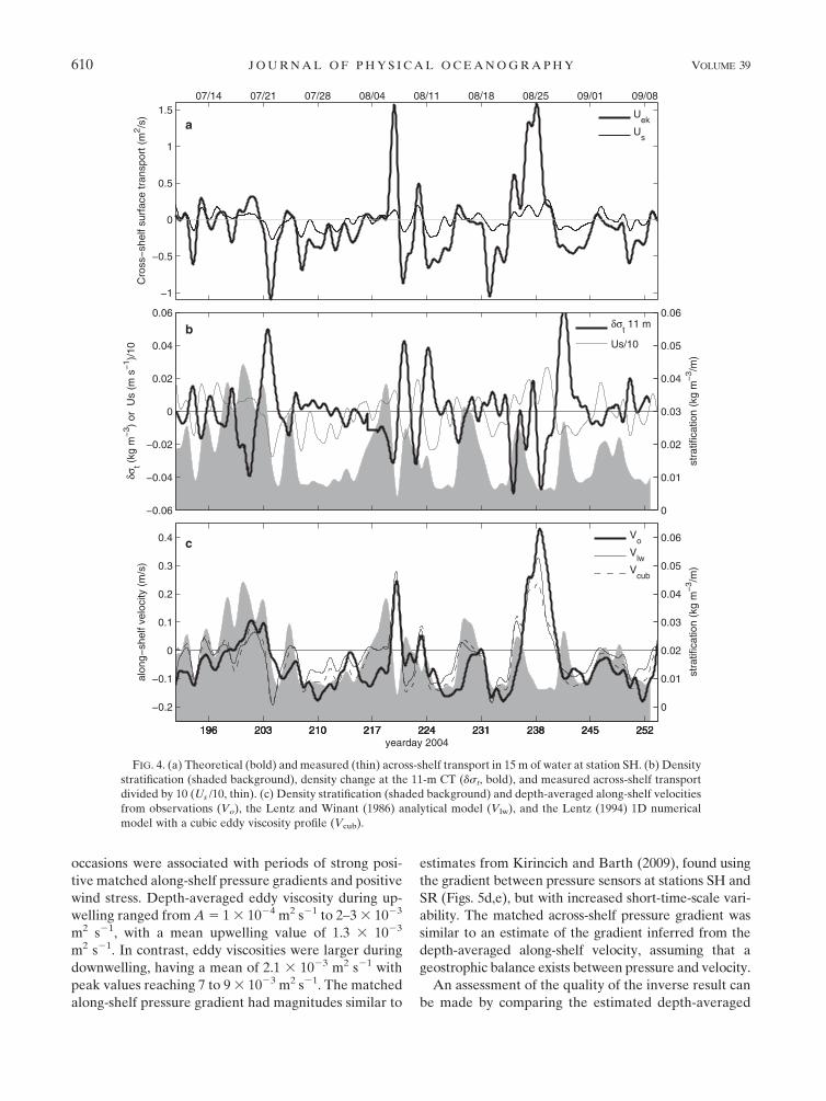
MARCH 2009 K I R I N C I C H A N D B A R T H 607
The time series of measured across-shelf surface trans-
port at SH was correlated with the theoretical Ekman
transport for the same period (0.73 at zero lag), but it
was lower in magnitude (Fig. 4a). Following the method
of Kirincich et al. (2005), the fraction of full theoretical
Ekman transport measured over the 60-day study pe-
riod was 25%. However, using this bulk calculation
technique over time scales similar to the 2–7-day wind
and stratification events yielded results that were not
statistically significant.
Given the small volume of water inshore of the 15-m
isobath, it is likely that this wind-forced across-shelf
transport was able to move water masses into and out of
the inner shelf on time scales similar to the fluctuating
FIG. 2. (a) Observed along-shelf wind stress at Newport with Acrobat section times marked by vertical lines with (b)
depth-averaged along- (bold) and across-shelf (thin) velocities, (c) temperature, and (d) density at station SH.
608 J O U R N A L O F P H Y S I C A L O C E A N O G R A P H Y VOLUME 39
winds. Assuming a simple mass conservation balance
between local density changes and the advection of a
density gradient by the across-shelf circulation, these
movements are illustrated by comparing the measured
surface transport to the density change at the 11-m
CT (Fig. 4b). Episodes of strong offshore (negative)
transport occur with positive density changes (e.g., days
203, 220, and 224), suggesting an onshore movement of
denser waters during active upwelling. The opposite was
true during transitions to downwelling events, with on-
shore (positive) surface transport occurring with nega-
tive density changes, or lighter waters entering the inner
shelf. Stratification (shaded in Fig. 4b) was most varia-
ble during these transitions, yet instances existed where
both surface transport and density change were large
but stratification was small (days 238–240), and where
surface transport was large but both density change and
stratification were small (e.g., days 207–212 and 232–233
in Fig. 4b). These findings appear to disagree with the
relationship between stratification and transport seen in
previous studies (Austin and Lentz 2002; Tilburg 2003;
Kirincich et al. 2005).
The forward models for along-shelf velocity intro-
duced earlier [section 2b(1)] are able to explain the
bulk of the velocity variability found at SH. Time series
of depth-averaged along-shelf velocities estimated for
the study period using these models, Vlw following
Lentz and Winant (1986) and Vcub following Lentz
(1994), were generally similar to and correlated with
(Vo/Vlw: 0.81 at zero lag, Vo/Vcub: 0.79 at zero lag)
measurements from station SH (Fig. 4c). However, the
model results failed to explain the variability of the
depth-averaged along-shelf velocity during periods of
increased or variable stratification. These times when
the modeled along-shelf velocities differed significantly
from observations (days 205–206, 215–220, 226–229, and
233–234) occurred when stratification was high or rap-
idly changing (Fig. 4c). Further, in agreement with Lentz
(1994), the 1D numerical model had difficulty repre-
senting the across-shelf circulation described above (not
shown here). Additional times of poor agreement (days
203–204 and 206–214) indicate that secondary forcings
(e.g., pressure gradients) may exist in addition to the
dominant wind forcing.
b. Estimated eddy viscosity
Similar to the observed variability described above,
the eddy viscosity (A) estimated using the inverse cal-
culation at station SH (Fig. 5) had a strong variability
(greater than two orders of magnitude) superimposed
on a mean value of 1.6 3 1023 m2 s21. Peak eddy vis-
cosities (.0.01 m2 s21) occurred during times of strong
surface forcing and rapidly changing stratification (e.g.,
days 222 and 237). At these times, eddy viscosity was a
maximum near the surface. Additional instances of el-
evated eddy viscosities occurred when A was a maxi-
mum near the bottom (e.g., days 195 and 207). These
FIG. 3. (a) Observed across-shelf hydrographic structure off-
shore of SH 15 on 10 August (day 223, dashed lines) and 11 August
(day 224, solid lines), (b) the geostrophic velocity [using Eq. (9)]
for 11 August, and (c) average northward velocities for 11 August
from R/V Elakha’s shipboard ADCP. In (b) and (c) southward
velocities (dashed) and northward velocities (solid) are marked
every 0.025 m s21, while the bold, solid line is the 0 m s21 contour.
MARCH 2009 K I R I N C I C H A N D B A R T H 609
occasions were associated with periods of strong posi-
tive matched along-shelf pressure gradients and positive
wind stress. Depth-averaged eddy viscosity during up-
welling ranged from A 5 1 3 1024 m2 s21 to 2–3 3 1023
m2 s21, with a mean upwelling value of 1.3 3 1023
m2 s21. In contrast, eddy viscosities were larger during
downwelling, having a mean of 2.1 3 1023 m2 s21 with
peak values reaching 7 to 9 3 1023 m2 s21. The matched
along-shelf pressure gradient had magnitudes similar to
estimates from Kirincich and Barth (2009), found using
the gradient between pressure sensors at stations SH and
SR (Figs. 5d,e), but with increased short-time-scale vari-
ability. The matched across-shelf pressure gradient was
similar to an estimate of the gradient inferred from the
depth-averaged along-shelf velocity, assuming that a
geostrophic balance exists between pressure and velocity.
An assessment of the quality of the inverse result can
be made by comparing the estimated depth-averaged
FIG. 4. (a) Theoretical (bold) and measured (thin) across-shelf transport in 15 m of water at station SH. (b) Density
stratification (shaded background), density change at the 11-m CT (dst, bold), and measured across-shelf transport
divided by 10 (Us /10, thin). (c) Density stratification (shaded background) and depth-averaged along-shelf velocities
from observations (Vo), the Lentz and Winant (1986) analytical model (Vlw), and the Lentz (1994) 1D numerical
model with a cubic eddy viscosity profile (Vcub).
610 J O U R N A L O F P H Y S I C A L O C E A N O G R A P H Y VOLUME 39
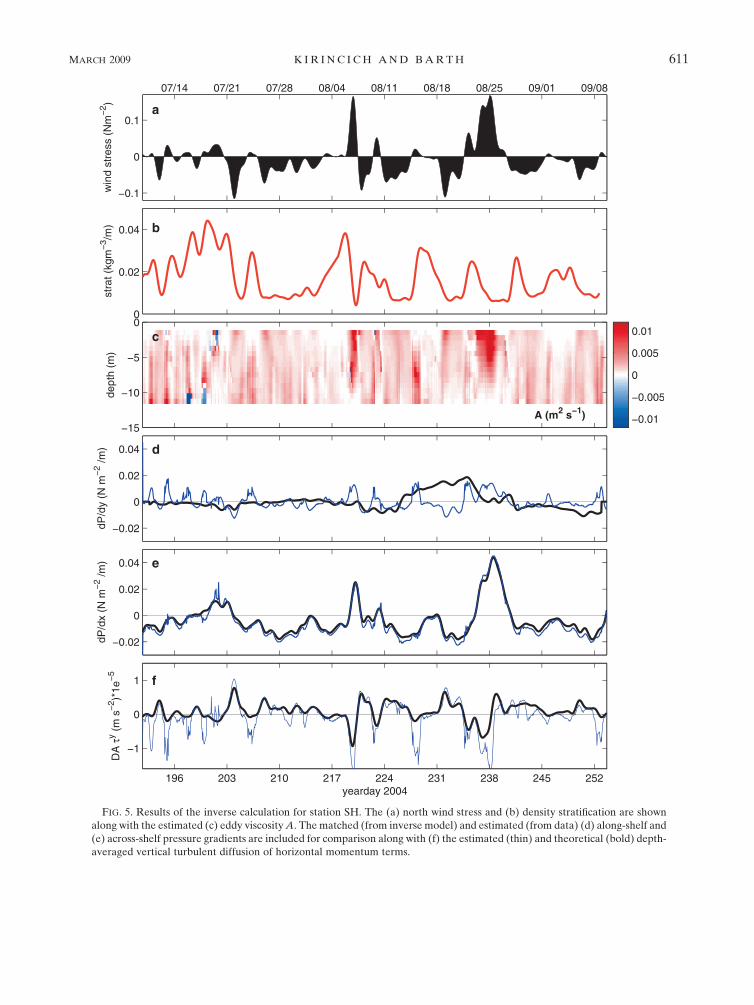
FIG. 5. Results of the inverse calculation for station SH. The (a) north wind stress and (b) density stratification are shown
along with the estimated (c) eddy viscosity A. The matched (from inverse model) and estimated (from data) (d) along-shelf and
(e) across-shelf pressure gradients are included for comparison along with (f) the estimated (thin) and theoretical (bold) depth-
averaged vertical turbulent diffusion of horizontal momentum terms.
MARCH 2009 K I R I N C I C H A N D B A R T H 611
along-shelf vertical diffusion term with its theoretical
equivalent, the sum of the wind stress and bottom stress
terms of the depth-averaged along-shelf momentum
equation:
1
H
ð0
�H
›
›zA
›y
›z
� �dz ;
(t sy � t b
y )
roH. (10)
Here, t by is a quadratic bottom stress, calculated using
the lowest velocity bin of the ADCP (2.5 m above the
bottom) and a drag coefficient of 1.5 3 1023 following
Perlin et al. (2005). In general, the two time series were
similar (Fig. 5f) and positively correlated (0.65). They
were most similar during upwelling-favorable winds,
with a correlation of 0.67, where the values shown in
Fig. 5f are mostly positive. The time series differed
substantially when the estimated term was negative
(Fig. 5f), which generally occurred during downwelling
wind events and/or times of positive along-shelf pres-
sure gradients. These discrepancies might be due to the
more barotropic flow conditions thought to be present
during downwelling or pressure-driven events. Here,
the majority of the vertical diffusion of turbulent mo-
mentum might occur closer to the bottom than the
lowest velocity measurement (Kirincich 2007). Thus,
this comparison is not entirely appropriate during these
types of conditions.
Based on these comparisons, the inverse calculation
appears to represent eddy viscosity sufficiently well,
particularly during upwelling-favorable winds. The dis-
crepancies that exist when A and velocity shear exceed
the thresholds described above were also times when the
forward models shown earlier did poorly. These periods
appear to be pressure forced, as the matched along-shelf
pressure gradient was large and positive (days 204, 215–
219, and 238 in Fig. 5d). However, a portion of the
matched gradient might also account for a discrepancy
between the forcing and the resulting velocity profiles, a
biased estimate of the mean vertical mixing term or a
significant depth-independent nonlinear term.
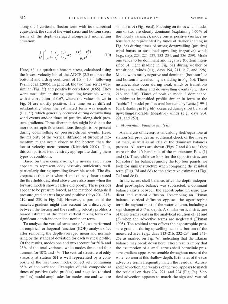
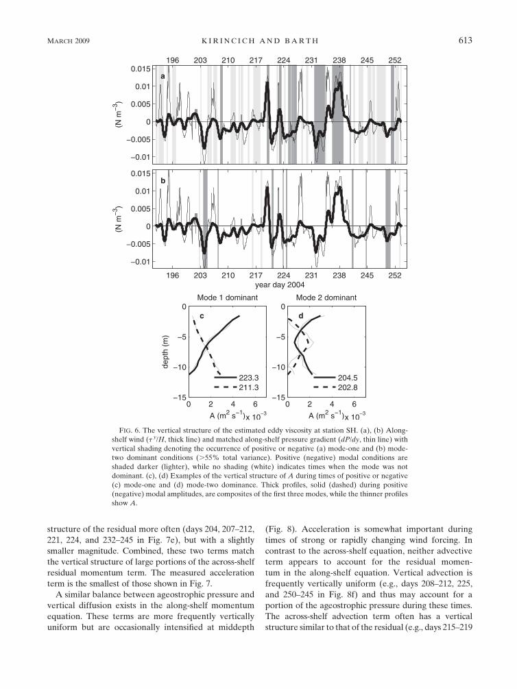
To analyze the vertical structure of A, we performed
an empirical orthogonal function (EOF) analysis of A
after removing the depth-averaged mean and normal-
izing by the standard deviation for each vertical profile.
Of the results, modes one and two account for 50% and
25% of the total variance, while modes three and four
account for 10% and 4%. The vertical structure of eddy
viscosity at station SH is well represented by a com-
posite of the first three modes, collectively containing
85% of the variance. Examples of this composite at
times of positive (solid profiles) and negative (dashed
profiles) modal amplitudes for modes one and two are
similar to A (Figs. 6c,d). Focusing on times when modes
one or two are clearly dominant (explaining .55% of
the hourly variance), mode one is positive (surface in-
tensified A; represented by times of darker shading in
Fig. 6a) during times of strong downwelling (positive)
wind bursts or sustained upwelling (negative) winds
(e.g., days 223, 225–227, 232–234, and 236–239). Mode
one tends to be dominant and negative (bottom inten-
sified A; light shading in Fig. 6a) during weaker or
transitional winds (e.g., days 194, 211, 217, and 228).
Mode two is rarely negative and dominant (both surface
and bottom intensified; light shading in Fig. 6b). These
instances also occur during weak winds or transitions
between upwelling and downwelling events (e.g., days
216 and 218). Times of positive mode 2 dominance,
a midwater intensified profile similar in form to the
‘‘cubic’’ A model profiles used here and by Lentz (1994)
(dark shading in Fig. 6b), occurred during short bursts of
upwelling-favorable (negative) winds (e.g., days 204,
221, and 250).
c. Momentum balance analysis
An analysis of the across- and along-shelf equations at
station SH provides an additional check of the inverse
estimate, as well as an idea of the dominant balances
present. All terms are shown (Figs. 7 and 8 ) as if they
were on the left-hand side of the momentum Eqs. (1)
and (2). Thus, while we look for the opposite structure
(or colors) for balances among the top four panels, we
look for similar structure when comparing the residual
term (Figs. 7d and 8d) to the advective estimates (Figs.
7e,f and 8e,f).
In the across-shelf balance, after the depth-indepen-
dent geostrophic balance was subtracted, a dominant
balance exists between the ageostrophic pressure gra-
dient and vertical diffusion. Resembling an Ekman
balance, vertical diffusion opposes the ageostrophic
term throughout most of the water column, including a
sign change at 5–7-m depth. A similar vertical structure
of these terms exists in the analytical solution of (1) and
(2) when the advective terms are neglected (Ekman
1905). The residual term offsets the ageostrophic pres-
sure gradient during upwelling near the bottom of the
measured area (e.g., days 213–216, 232–234, and 241–
252 as marked on Fig. 7e), indicating that the Ekman
balance may break down here. These results imply that
the assumption of a small across-shelf baroclinic pres-
sure gradient appears reasonable throughout most of the
water column at this shallow depth. Estimates of the two
advective terms frequently match the residual. Across-
shelf advection, the weaker of the two, appears to match
the residual on days 204, 221, and 224 (Fig. 7e). Ver-
tical advection appears to match the sign and vertical
612 J O U R N A L O F P H Y S I C A L O C E A N O G R A P H Y VOLUME 39
structure of the residual more often (days 204, 207–212,
221, 224, and 232–245 in Fig. 7e), but with a slightly
smaller magnitude. Combined, these two terms match
the vertical structure of large portions of the across-shelf
residual momentum term. The measured acceleration
term is the smallest of those shown in Fig. 7.
A similar balance between ageostrophic pressure and
vertical diffusion exists in the along-shelf momentum
equation. These terms are more frequently vertically
uniform but are occasionally intensified at middepth
(Fig. 8). Acceleration is somewhat important during
times of strong or rapidly changing wind forcing. In
contrast to the across-shelf equation, neither advective
term appears to account for the residual momen-
tum in the along-shelf equation. Vertical advection is
frequently vertically uniform (e.g., days 208–212, 225,
and 250–245 in Fig. 8f) and thus may account for a
portion of the ageostrophic pressure during these times.
The across-shelf advection term often has a vertical
structure similar to that of the residual (e.g., days 215–219
FIG. 6. The vertical structure of the estimated eddy viscosity at station SH. (a), (b) Along-
shelf wind (t y/H, thick line) and matched along-shelf pressure gradient (dP/dy, thin line) with
vertical shading denoting the occurrence of positive or negative (a) mode-one and (b) mode-
two dominant conditions (.55% total variance). Positive (negative) modal conditions are
shaded darker (lighter), while no shading (white) indicates times when the mode was not
dominant. (c), (d) Examples of the vertical structure of A during times of positive or negative
(c) mode-one and (d) mode-two dominance. Thick profiles, solid (dashed) during positive
(negative) modal amplitudes, are composites of the first three modes, while the thinner profiles
show A.
MARCH 2009 K I R I N C I C H A N D B A R T H 613
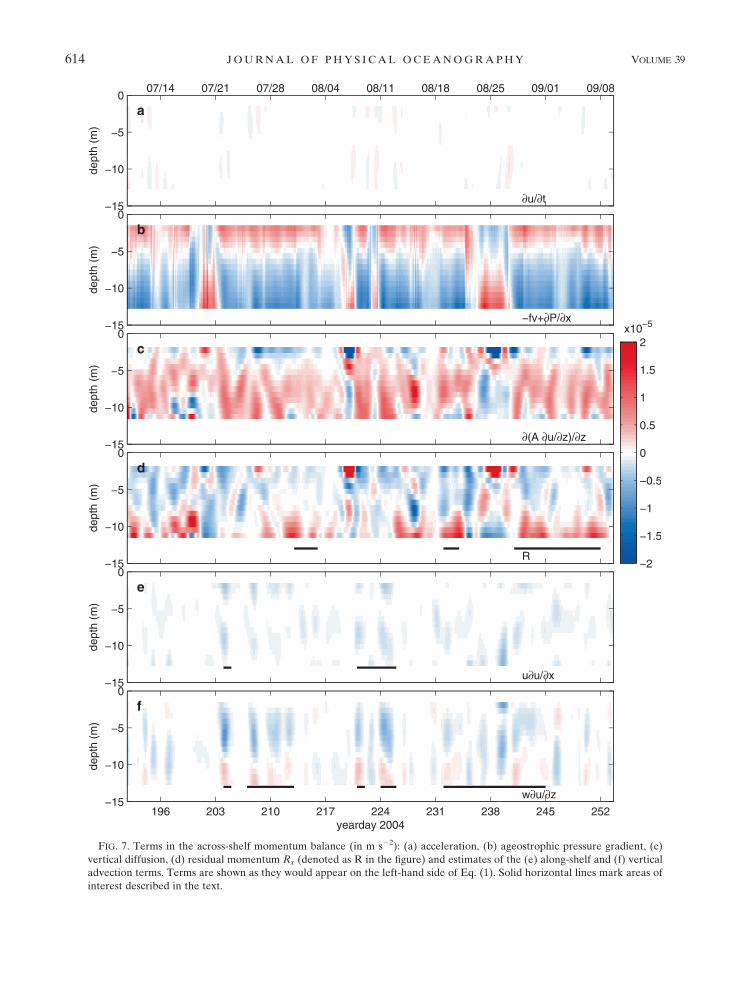
FIG. 7. Terms in the across-shelf momentum balance (in m s22): (a) acceleration, (b) ageostrophic pressure gradient, (c)
vertical diffusion, (d) residual momentum Rx (denoted as R in the figure) and estimates of the (e) along-shelf and (f) vertical
advection terms. Terms are shown as they would appear on the left-hand side of Eq. (1). Solid horizontal lines mark areas of
interest described in the text.
614 J O U R N A L O F P H Y S I C A L O C E A N O G R A P H Y VOLUME 39
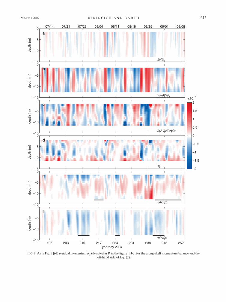
FIG. 8. As in Fig. 7 [(d) residual momentum Ry (denoted as R in the figure)], but for the along-shelf momentum balance and the
left-hand side of Eq. (2).
MARCH 2009 K I R I N C I C H A N D B A R T H 615
and 241–252 in Fig. 8e), but of opposite sign. This might
occur if the core of the along-shelf velocity jet associated
with this small-scale upwelling circulation (Kirincich and
Barth 2009) was inshore of station SH, reversing the
gradient shown.
Spikes or sharp sign changes in vertical diffusion oc-
cur in both momentum equations and generally coin-
cide with opposing patterns in the residual momentum
terms. Occurring most frequently during times of rapid
transitions between upwelling and downwelling (days
198, 200, 206, 227, and 246), these patterns are the
largest magnitude features for each term and further
indicate the effects of measurement or calculation er-
rors. In both equations, the residual tends to be highest
in the bottom of the measured area where calculation
errors are largest (Kirincich 2007). Despite these dis-
crepancies, the comparisons highlighted above provide
additional support of the vertical diffusion and eddy
viscosity estimated from the inverse calculation, and they
help infer the sources of the residual momentum terms.
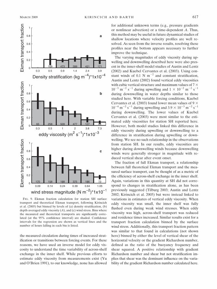
d. Across-shelf exchange efficiency
Previous studies have found links between the level of
stratification present and the across-shelf exchange ef-
ficiency (Austin and Lentz 2002; Kirincich et al. 2005),
but the observations of event-scale variations shown
earlier do not reveal such a pattern. To explore this
further, we computed the Ekman transport fraction,
following Kirincich et al. (2005), for varying levels of
stratification. Separating the time series of theoretical
and measured transports into six equally sized bins,
based on the logarithm of stratification, and computing
the transport fraction for each bin leads to statistically
significant results (Fig. 9a). The resulting mean Ekman
transport fraction is similar for all levels of stratification,
and thus no real trend exists that supports a link be-
tween transport fraction and stratification.
In contrast, a similar binned Ekman transport fraction
calculation using depth-averaged A, instead of stratifi-
cation, gives drastically different results. Here, the
fraction of full Ekman transport decreases as the mag-
nitude of A increases (Fig. 9b). Of the significant
(shaded) results, Ekman transport ranged from 60% for
A 5 0.3 3 1023 m2 s21 to 15% for A 5 3.8 3 1023
m2 s21. The majority of the measurements fell in the
band between fractions of 37% and 30% and A 5 1 to 2
3 1023 m2 s21. The median fraction given here was 10%
higher than the time series mean fraction noted earlier.
A third calculation, binned by the surface wind stress,
has a trend similar to that of eddy viscosity. The fraction
of full Ekman transport decreases as the magnitude of
the wind stress increases (Fig. 9c), from 65% for stresses
under 1 3 1023 N m22 to 25% at stresses of 0.1 N m22.
The distribution of these transport fractions, binned
by A, during the 8-day period starting on yearday 218
illustrates how the fraction of full Ekman transport
varies with forcing events. The lowest fractions occurred
during the peak downwelling event of day 219 (Fig. 10),
while the highest fractions occurred at times of weaker
wind forcing or event transitions (days 218, 222.3, and
223). This variability can also be thought of as more
(high fraction) or less (low fraction) of the Ekman spiral
fitting into the water column as conditions vary in time.
The progression of high fractions to low fractions and
back over the course of a wind event is illustrated by the
upwelling events present in this time period (Fig. 10).
This is of particular importance because the fractional
transport can be large in the initial or final stages of a
wind event, presumably as the water column is more
stratified. It is during these times that the total exchange
of the inner-shelf water masses is likely to occur.
In general, downwelling events tend to have lower
transport fractions than upwelling events, or a weaker
across-shelf transport relative to wind forcing. An anal-
ysis of average upwelling and downwelling characteristics
after event onset revealed two key differences responsi-
ble for the lower fractions seen during downwelling.
First, downwelling events tend to have stronger peak
winds than upwelling events. Second, and perhaps more
importantly, during downwelling the vertical shear of
the horizontal velocity was reduced after event onset
relative to upwelling. Through the inverse model, these
factors contributed to higher eddy viscosities and thus
reduced transport fractions during downwelling. This
discrepancy has important implications for across-shelf
transport in the inner shelf. As illustrated in the bottom
of Fig. 10, the across-shelf transport accumulated over
the 8-day period was more negative than the theoretical
transport reduced by the mean transport fraction
(25%). This difference is due to reduced transport
during the first downwelling event as well as increased
transport during upwelling and event transitions. As a
result, twice as much water was upwelled through the
region inshore of the mooring over the 8-day period
than that predicted using the mean transport fraction.
4. Discussion
Conditions at station SH were dominated by rapid
and short fluctuations between upwelling and down-
welling, with upwelling events averaging 40 h in length
and downwelling events averaging 30 h in length. Per-
haps because of these short-time-scale variations, the
expected relationship between stratification and trans-
port fraction was not seen. Additionally, simple wind-driven
velocity models were not able to accurately represent
616 J O U R N A L O F P H Y S I C A L O C E A N O G R A P H Y VOLUME 39
the measured circulation during times of increased strat-
ification or transitions between forcing events. For these
reasons, we have used an inverse model for eddy vis-
cosity to understand the time variability of across-shelf
exchange in the inner shelf. While previous efforts to
estimate eddy viscosity from measurements exist (Yu
and O’Brien 1991), to our knowledge, none has allowed
for additional unknown terms (e.g., pressure gradients
or nonlinear advection) or a time-dependent A. Thus,
this method may be useful in future dynamical studies of
shallow locations where velocity profiles are well re-
solved. As seen from the inverse results, resolving these
profiles near the bottom appears necessary to further
improve the technique.
The varying magnitudes of eddy viscosity during up-
welling and downwelling described here were also pres-
ent in the inner-shelf model studies of Austin and Lentz
(2002) and Kuebel Cervantes et al. (2003). Using con-
stant winds of 0.1 N m22 and constant stratification,
Austin and Lentz (2002) found vertical eddy viscosities
with cubic vertical structure and maximum values of 7 3
1023 m22 s21 during upwelling and 1 3 1022 m22 s21
during downwelling in water depths similar to those
studied here. With variable forcing conditions, Kuebel
Cervantes et al. (2003) found lower mean values of 9 3
1024 m22 s21 during upwelling and 3.9 3 1023 m22 s21
during downwelling. The lower values of Kuebel
Cervantes et al. (2003) were most similar to the esti-
mated eddy viscosities for station SH reported here.
However, both model studies linked this difference in
eddy viscosity during upwelling or downwelling to a
difference in stratification during upwelling or down-
welling. We see no such relationship in the observations
from station SH. In our results, eddy viscosities are
higher during downwelling winds because downwelling
winds were generally stronger in magnitude with re-
duced vertical shear after event onset.
The fraction of full Ekman transport, a relationship
between full theoretical Ekman transport and the mea-
sured surface transport, can be thought of as a metric of
the efficiency of across-shelf exchange in the inner shelf.
Again, variations in this quantity at SH did not corre-
spond to changes in stratification alone, as has been
previously suggested (Tilburg 2003; Austin and Lentz
2002; Kirincich et al. 2005) but were instead linked to
variations in estimates of vertical eddy viscosity. When
eddy viscosity was small, the inner shelf was fully
flushed even during weak wind stresses. When eddy
viscosity was high, across-shelf transport was reduced
and residence times increased. Similar results exist for a
transport fraction calculation binned by the surface
wind stress. Additionally, this transport fraction pattern
was similar to that found in calculations (not shown
here) binned by either the level of vertical shear of the
horizontal velocity or the gradient Richardson number,
defined as the ratio of the buoyancy frequency and
shear squared. A positive relationship with gradient
Richardson number and shear but not stratification im-
plies that shear was the dominant influence on the varia-
bility of the gradient Richardson number calculated here.
FIG. 9. Ekman fraction calculation for station SH surface
transport and theoretical Ekman transport, following Kirincich
et al. (2005) but binned by levels of (a) density stratification, (b)
depth-averaged eddy viscosity (A), and (c) wind stress. Bins where
the measured and theoretical transports are significantly corre-
lated (at the 95% confidence interval) are shaded. Confidence
intervals for the regression are shown as vertical lines and the
number of hours falling in each bin is listed.
MARCH 2009 K I R I N C I C H A N D B A R T H 617
As wind stress and velocity shear are inputs to the in-
verse model, it is perhaps not surprising that their effect
on the efficiency of across-shelf exchange is similar to
that of eddy viscosity. It is of interest that no clear rela-
tionship between stratification and the transport fraction
was found here. Given that our observations are domi-
nated by rapid variations in conditions driven by short-
time-scale fluctuations of the wind forcing, we infer that
wind forcing and velocity shear set the eddy viscosity,
and thus the transport fraction, during these transitional
periods. The effects of stratification on across-shelf ex-
change may be more important after the forcing has
been sustained for a number of inertial periods. How-
ever, given the uncertainty existing in the inverse results,
more work is needed to fully understand this difference.
Our results illustrate that northward downwelling-
favorable wind bursts lead to high eddy viscosities and
low amounts of across-shelf transport. Thus, the net
across-shelf circulation can be biased toward the up-
welling of colder, nutrient-rich waters into the inner
shelf during periods of fluctuating wind forcing. This
result has significant implications for the common use of
large-scale, wind-based upwelling indices to estimate
coastal upwelling. Although the total magnitude of
upwelled waters, integrated across the shelf, might be
accurately predicted with such indices, the amount of
upwelled waters seen at a particular across-shelf loca-
tion in the inner shelf may vary greatly from the index.
In particular, these indices will underestimate the net
water upwelled inshore of a given water depth during
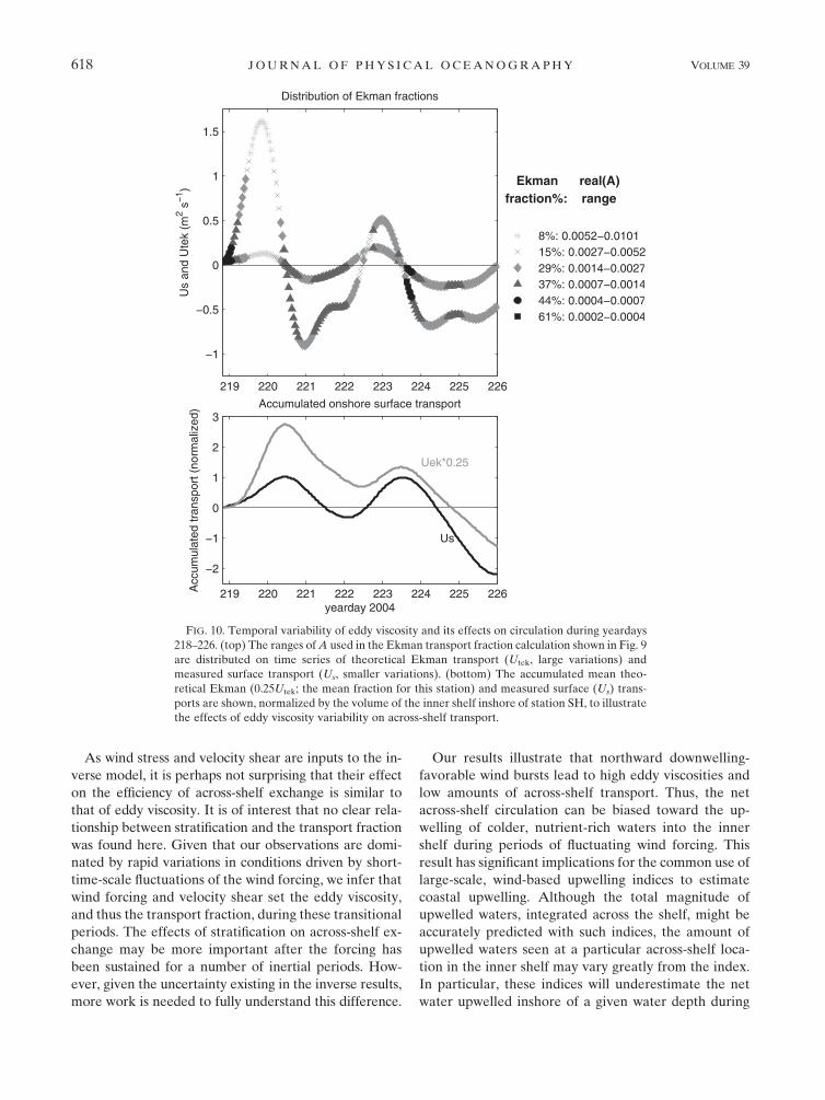
FIG. 10. Temporal variability of eddy viscosity and its effects on circulation during yeardays
218–226. (top) The ranges of A used in the Ekman transport fraction calculation shown in Fig. 9
are distributed on time series of theoretical Ekman transport (Utek, large variations) and
measured surface transport (Us, smaller variations). (bottom) The accumulated mean theo-
retical Ekman (0.25Utek; the mean fraction for this station) and measured surface (Us) trans-
ports are shown, normalized by the volume of the inner shelf inshore of station SH, to illustrate
the effects of eddy viscosity variability on across-shelf transport.
618 J O U R N A L O F P H Y S I C A L O C E A N O G R A P H Y VOLUME 39
periods of variable wind forcing. We believe this result
is most applicable to inner-shelf areas where the across-
shelf transport is tightly correlated with the measured
winds and both upwelling and downwelling events
commonly occur. This result may be complicated, or
confounded, by additional forcings (e.g., along-shelf
pressure gradients) or spatial variations in circulation.
The analysis of the along- and across-shelf momen-
tum equations pointed to possible sources for the re-
sidual momentum terms. The Ekman balance appeared
to occasionally break down near the bottom of the
water column as the residual term, and not vertical
diffusion, opposed the vertical shear of the horizontal
velocity in these areas. The baroclinic pressure gradient,
observed offshore of 15 m both here and in previous
inner-shelf studies (Lentz et al. 1999; Garvine 2004) but
not included in the inverse formulation, is a likely
source for this residual momentum. Additionally, esti-
mates of along-shelf and vertical advection matched the
remaining vertical structure of the residual term in the
across-shelf equation. In the along-shelf momentum
equation, the potential for these terms to account for
the remaining residual momentum was less clear. The
importance of across-shelf advection in balancing ver-
tical diffusion in the along-shelf momentum equation
during active upwelling was shown by Kuebel Cervantes
et al. (2003) and Lentz and Chapman (2004). However,
our estimate for this term was similar in structure to the
residual, but opposite in sign, perhaps suggesting an
error in the assumptions made in its calculation. Despite
these similarities, the inclusion of these estimates for the
advective terms in the inverse calculation did not sig-
nificantly alter estimates of A or reduce Rx and Ry
(Kirincich 2007). Thus, it appears that better estimates
of these terms are necessary in future studies to fully
understand the time variability of this system.
The episodes of total water mass exchange and the pro-
gression of transport efficiency during wind events identi-
fied in this study may have significant implications for
inner-shelf ecological communities. Previous ecological
studies in upwelling environments show that increased
settlement of larval invertebrates was correlated with epi-
sodes of increasing water temperatures (Miller and Emlet
1997; Farrell et al. 1991; Broitman et al. 2005). Along the
Oregon coast, the transition from upwelling to downwel-
ling, with its decreased eddy viscosity and increased across-
shelf transport efficiency, allows for a full flushing of the
inner shelf and replacement with warm, fresh surface
water. Once this transition has occurred, eddy viscosity
increases and across-shelf circulation is reduced or shut
down. This process provides a mechanism for focused,
successful across-shelf transport or retention of propa-
gules. Whether this aids recruitment depends on the life
cycle characteristics of the individual species. Larvae
released during such an event would tend to stay closer
to shore for a longer period of time than if released
during normal upwelling conditions. Additionally, with
an overall bias toward onshore transport at depth during
upwelling, larvae able to adjust their buoyancy might be
able to move onshore in a predicable manner.
5. Conclusions
This analysis has described the short-time-scale (2–7
day) variability of forcing, circulation, and hydrography
along the central Oregon coast. Conditions in the study
area, sheltered from the regional circulation by an off-
shore submarine bank, were highly variable in time.
With the local circulation driven by along-shelf wind
forcing, rapid transitions occurred between upwelling
and downwelling events and a variety of water masses
occupied the inner shelf. To understand this variability,
we adapted a simple one-dimensional numerical model
to estimate the time-dependent vertical eddy viscosity, a
parameterization of the transfer of momentum due to
turbulent eddies, from typical observations of velocity
and wind forcing. The novelty of the inverse method
was that it estimated eddy viscosity while allowing for
additional unknown sources of momentum.
With the results of this inverse calculation, we were
able to quantify the effects of variable forcing on across-
shelf exchange. The estimated eddy viscosity varied
over time scales similar to forcing events, averaging
1.3 3 1023 m2 s21 during upwelling winds and 2.1 3
1023 m2 s21 during downwelling winds. The fraction of
full Ekman transport present in the surface layer, a
measure of the efficiency of across-shelf exchange at this
water depth, was a strong function of the eddy viscosity
and wind forcing but not stratification. Transport frac-
tions ranged from 60% during times of weak or variable
wind forcing and low eddy viscosity, to 10%–20% dur-
ing times of strong downwelling and high eddy viscosity.
The increased eddy viscosity and decreased exchange ef-
ficiency found during downwelling events was linked to
reduced vertical shear of the horizontal velocity during
downwelling events, not to reductions in stratification.
These trends result from the rapid fluctuations between
upwelling and downwelling and the relatively short dura-
tion of these events, allowing wind stress and velocity shear
to dominate the vertical diffusion. Previous model and
observational results finding stronger links between strati-
fication and exchange efficiency were focused on the effects
of constant wind forcing or seasonal mean circulation.
The difference in eddy viscosities between upwelling and
downwelling led to varying across-shelf exchange efficien-
cies and, potentially, increased net upwelling over time.
MARCH 2009 K I R I N C I C H A N D B A R T H 619
Acknowledgments. This paper is Contribution Num-
ber 310 from PISCO, the Partnership for Interdiscipli-
nary Studies of Coastal Oceans, funded primarily by the
Gordon and Betty Moore Foundation and the David and
Lucile Packard Foundation. We thank J. Lubchenco and
B. Menge for establishing and maintaining the PISCO
observational program at OSU. We also thank Captain
P. York, C. Holmes, and S. Holmes for their data col-
lection efforts, B. Kuebel Cervantes for providing the
model output used to test the inverse method, and
M. Levine (OSU) and S. Lentz (WHOI) for helpful com-
ments on the manuscript.
REFERENCES
Austin, J., and S. Lentz, 2002: The inner shelf response to wind-driven
upwelling and downwelling. J. Phys. Oceanogr., 32, 2171–2193.
Barth, J., S. Pierce, and T. Cowles, 2005: Mesoscale structure and
its seasonal evolution in the northern California Current
System. Deep-Sea Res. II, 52, 5–28.
Broitman, B., C. Blanchette, and S. Gaines, 2005: Recruitment of
intertidal invertebrates and oceanographic variability at Santa
Cruz Island, California. Limnol. Oceanogr., 50, 1473–1479.
Chelton, D., 1983: Effects of sampling errors in statistical estima-
tion. Deep-Sea Res., 30, 1083–1101.
Ekman, V., 1905: On the influence of the Earth’s rotation on
ocean-currents. Arkiv. Math. Astro. Fys., 2, 1–53.
Farrell, T., D. Bracher, and J. Roughgarden, 1991: Cross-shelf
transport causes recruitment to intertidal populations in
central California. Limnol. Oceanogr., 36, 279–288.
Garvine, R., 2004: The vertical structure and subtidal dynamcis of
the inner shelf off New Jersey. J. Mar. Res., 62, 337–371.
Kirincich, A., 2003: The structure and variability of a coastal
density front. M.S. thesis, Graduate School of Oceanography,
University of Rhode Island, 124 pp.
——, 2007: Inner-shelf circulation off the central Oregon coast.
Ph.D. dissertation, Oregon State University, 179 pp.
——, and J. Barth, 2009: Alongshelf variability of inner-shelf cir-
culation along the central Oregon coast during summer.
J. Phys. Oceanogr., in press.
——, ——, B. Grantham, B. Menge, and J. Lubchenco, 2005: Wind-
driven inner-shelf circulation off central Oregon during sum-
mer. J. Geophys. Res., 110, C10S03, doi:10.1029/2004JC002611.
Kuebel Cervantes, B., J. Allen, and R. Samelson, 2003: A mod-
eling study of Eulerian and Lagrangian aspects of shelf cir-
culation off Duck, North Carolina. J. Phys. Oceanogr., 33,
2070–2092.
Lentz, S., 1994: Current dynamics over the northern California
inner shelf. J. Phys. Oceanogr., 24, 2461–2478.
——, 1995: Sensitivity of the inner-shelf circulation to the form of
the eddy viscosity profile. J. Phys. Oceanogr., 25, 19–28.
——, 2001: The influence of stratification on the wind-driven
cross-shelf circulation over the North Carolina shelf. J. Phys.
Oceanogr., 31, 2749–2760.
——, and C. Winant, 1986: Subinertial currents on the southern
California shelf. J. Phys. Oceanogr., 16, 1737–1750.
——, and D. Chapman, 2004: The importance of nonlinear cross-
shelf momentum flux during wind-driven coastal upwelling.
J. Phys. Oceanogr., 34, 2444–2457.
——, R. Guza, S. Elgar, F. Feddersen, and T. Herbers, 1999:
Momentum balances on the North Carolina inner shelf.
J. Geophys. Res., 104, 18 205–18 226.
Mellor, G., and T. Yamada, 1982: Development of a turbulence
closure model for geophysical fluid problems. Rev. Geophys.
Space Phys., 20, 851–875.
Miller, B., and R. Emlet, 1997: Influence of nearshore hydrody-
namics on larval abundance and settlement of sea urchins
Stronglocentrotus franciscanus and S. purpuratus in the
Oregon upwelling zone. Ecol. Prog. Ser., 148, 83–94.
Panchang, V., and J. Richardson, 1993: Inverse adjoint estimation
of eddy viscosity for coastal flow models. J. Hydrol. Eng., 119,
506–524.
Pawlowicz, R., B. Beardsley, and S. Lentz, 2002: Classical tidal
harmonic analysis including error estimates in MATLAB
using T2TIDE. Comput. Geosci., 28, 929–937.
Perlin, A., J. Moum, J. Klymak, M. Levine, T. Boyd, and P. Kosro,
2005: A modified law-of-the-wall applied to oceanic bottom
boundary layers. J. Geophys. Res., 110, C10S10, doi:10.1029/
2004JC002310.
Samelson, R., and Coauthors, 2002: Wind stress forcing of the
Oregon coastal ocean during the 1999 upwelling season.
J. Geophys. Res., 107, 3034, doi:10.1029/2001JC000900.
Signell, R., R. Beardsley, H. Graber, and A. Capotondi, 1990: Effect
of wave-current interaction on wind-driven circulation in nar-
row, shallow embayments. J. Geophys. Res., 95, 9671–9678.
Tilburg, C., 2003: Across-shelf transport on a continental shelf: Do
across-shelf winds matter? J. Phys. Oceanogr., 33, 2675–2688.
Wiseman, W., and R. Garvine, 1995: Plumes and coastal currents
near large river mouths. Estuaries, 18, 509–517.
Yankovsky, A., R. Garvine, and A. Munchow, 2000: Mesoscale
currents on the inner New Jersey shelf driven by the inter-
action of buoyancy and wind forcing. J. Phys. Oceanogr., 5,2214–2230.
Yu, L., and J. O’Brien, 1991: Variational estimation of the wind stress
drag coefficient and oceanic eddy viscosity profile. J. Phys.
Oceanogr., 21, 709–719.
620 J O U R N A L O F P H Y S I C A L O C E A N O G R A P H Y VOLUME 39
Related Documents


