Time Structure of Observed, GCM-Simulated, … OCTOBER 2001 HUTH ET AL. 4047 Time Structure of Observed, GCM-Simulated, ~Downscaled, and Stochastically Generated Daily Temperature

15 OCTOBER 2001 HUTH ET AL. 4047

Time Structure of Observed, GCM-Simulated, ~Downscaled, andStochastically Generated Daily Temperature Series

RADAN HUTH

Institute of Atmospheric Physics, Prague, Czech Republic

IAN KYSELY

Institute of Atmospheric Physics, and Department of Meteorology and Environment Protection, Charles University,Prague, Czech Republic

MARTIN DUBROVSKY

Institute of Atmospheric Physics, Prague, Czech Republic

(Manuscript received 7 September 2000, in final form 20 February 2001)

ABSTRACT

The time structure of simulated daily maximum and minimum temperature series, produced by several differentmethods, is compared with observations at six stations in central Europe. The methods are statistical downscaling,stochastic weather generator, and general circulation models (GCMs). Outputs from control runs of two GCMsare examined: ECHAM3 and CCCM2. Four time series are constructed by statistical downscaling-using multiple

linear regression of 500-hPa heights and 1000-/500-hPa thickness: (i) from observations with variance reproducedby the inflation technique, (ii) from observations with variance reproduced by adding a white noise process,and (iii) from the two GCMs. Two runs of the weather generator were performed, one considering and oneneglecting the annual cycle of lag-O and lag-l correlations among daily weather characteristics. Standard deviationand skewness of day-to-day temperature changes and lag-l autocorrelations are examined. For heat and coldwaves, the occurrence frequency, mean duration, peak temperature, and mean position within the year are studied.

Possible causes of discrepancies between the simulated and observed time series are discussed and identified.They are shown to stem, among others, from (i) the absence of physics in downscaled and stochastically generatedseries, (ii) inadequacies of treatment of physical processes in GCMs, (iii) assumptions of linearity in downscalingequations, and (iv) properties of the underlying statistical model of the weather generator. In downscaling,variance inflation is preferable to the white noise addition in most aspects as the latter results in highly over-estimated day-to-day variability. The inclusion of the annual cycle of correlations into the weather generatordoes not lead to an overall improvement of the temperature series produced. None of the methods appears tobe able to reproduce all the characteristics of time structure correctly.

I

1. Introduction

Studies of climate change impacts frequently requiredaily time series of climate variables such as tempera-ture and precipitation for a future climate state at aspecific site. There are several ways of obtaining site-specific daily time series, which are to a different extentbased on general circulation model (GCM) outputs(Giorgi and Mearns 1991; Kattenberg et al. 1996; Dub-rovsky 1997). Those frequently used include taking theGCM output itself, regional climate models (RCMs),statistical downscaling, and weather generators. In orderto have confidence in simulations of a future climate,

Corresponding author address: Dr. Radan Huth, Institute of At-mospheric Physics, Bocnf II 1401, 141 31 Prague, Czech Republic.E-mail: [email protected]

@ 2001 American Meteorological Society

we must verify that the particular method is capable ofsimulating present climate conditions reliably. In thispaper, we concentrate on the evaluation of simulationsof present climate by several methods of producing site-specific daily temperature series; we do not deal withapplications of the methods to future climate conditions.The latter subject is discussed, for example, in Hulmeet al. (1994) for the use of a direct GCM output; in Hayet al. (2000) for a direct GCM output and downscaling;in Winkler et al. (1997) and Huth and Kysely (2000)for downscaling; and in Semenov and Barrow (1997)and Dubrovsky et al. (2000) for weather generators.

Many studies evaluate the performance of the above-mentioned approaches against observed data, but thevast majority concerns a single method only. A simul-taneous use of several methods and a subsequent com-parison would, nevertheless, aid in selecting the most

4048 JOURNAL OF CLIMATE VOLUME 14

appropriate technique for specific applications in futurestudies. There are only few studies that attempted tomake such a comparison for daily temperature. Kidsonand Thompson (1998) compared statistical downscalingwith a limited-area model over New Zealand, arrivingat the conclusion that both methods perform with a sim-ilar accuracy. Hay et al. (2000) found that downscalingfrom observations approximates daily temperatures inselected North American basins better than a directGCM output and downscaling from GCM.

In most studies, simulated time series are verifiedagainst observations in terms of distance measures suchas root-mean-square error and correlation coefficient,and in terms of the first two statistical moments, thatis, the mean and standard deviation. These are, however,only a few of the possible criteria. In many applications,for example, in crop growth modeling, the reliability ofthe time structure of a series is of crucial importance.In spite of this, little has been done in examining thetime structure of temperature series produced by variousmethods. Several studies investigated autocorrelationsof temperature series in GCM and RCM outputs (Buis-hand and Beersma 1993; Mearns et al. 1995; Kalvovaand Nemesova 1998) and the occurrence of prolongedextreme events, such as heat waves (Huth et al. 2000).No study has so far analyzed the time structure of down-scaled temperature series, except for Trigo and Palutikof(1999) who examined the numbers of heat and coldwaves. Hayhoe (2000) validated the weather generatorin terms of the distribution of the length of frost-freeperiods.

The aim of this study is to analyze time series of dailyextreme temperatures produced by two GCMs, a statis-tical downscaling procedure, and a weather generator,and verify them against observations at six central Eu-ropean sites. The analysis is focused on empirical dis-tributions of day-to-day temperature changes and, pri-marily, on prolonged periods of high and low temper-atures, that is, heat and cold waves. Although extremeevents have recently begun to playa more importantrole in analyses of climate change simulations (Meehlet al. 2000), little attention has so far been paid to heatand cold waves. We also examine the effect on timeseries of (i) the way the variance is reproduced in sta-tistical downscaling and (ii) whether the annual cycleof correlations and lagged correlations among simulatedvariables is implemented in the weather generator ornot.

2. Datasets and methods of their construction

a. GCMs

The simulations of present climate (control runs) oftwo GCMs have been used in this study. The ECHAMGCM originates from the European Centre for Medium-Range Weather Forecasts model-hence EC, modifiedby the Max Planck Institute for Meteorology in Ham-

burg, Germany-hence HAM. A detailed description ofits version 3, used here, is given in Deutsches Klima-rechenzentrum (DKRZ 1993). It has a T42 resolution,corresponding approximately to a 2.8° grid spacing bothin longitude and latitude. Here we examine years 11-40 of the control run, in which climatological SSTs andsea ice were employed. The validation of daily extremetemperatures produced by ECHAM was performed forselected areas of the Czech Republic by Nemesova andKalvova (1997) and Nemesova et al. (1998).

The Canadian Climate Centre Model (CCCM) of thesecond generation is described in McFarlane et al.(1992) where also its basic validation is presented. TheCCCM model has a T32 resolution, roughly correspond-ing to a 3.75° X 3.75° grid. Its interactive lower bound-ary consists of a mixed layer ocean model and a ther-modynamic ice model. Twenty years of its control in-tegration have been available. The validation of its sur-face temperature characteristics over central Europe wasperformed by Kalvova et al. (2000).

There is a continuing debate as to whether GCM out-puts should be treated as gridbox or gridpoint values(Skelly and Henderson-Sellers 1996), that is, if the grid-ded output of a model should be compared with indi-vidual station values or areal aggregates (e.g., spatialmeans). Huth et al. (2000) have shown that for dailymaximum temperatures and heat waves, there is virtu-ally no difference between the two approaches, and agrid point versus station comparison is thus justified.Therefore, we compare temperature characteristics atindividual stations with GCM outputs at the grid pointsclosest to them.

b. Downscaling

Downscaled temperatures were calculated by multiplelinear regression with stepwise screening from gridded500-hPa heights and 1O00-/500-hPa thickness over thedomain covering most of Europe and extending overthe adjacent Atlantic Ocean (bounded by 32.1°, 65.6°N,16.9°W,and 28.1°E). The stepwise regression of griddedvalues was selected because in the intercomparisonstudy by Huth (1999), it turned out to perform bestamong other linear methods, including regression ofprincipal components and canonical correlation analy-sis. In that study, a detailed description of the procedurecan be found, including the selection of the most in-formative predictors.

The downscaling procedure is designed so that it re-tains the mean of the original time series. It is importantto retain also variance; there are two possible ways ofdoing that, which are both applied and compared in thisstudy. The commonly used way, variance inflation, con-sists in enhancing each day's anomaly by the same fac-tor, defined by the share of variance explained by down-scaling (Karl et al. 1990). However, the variance infla-tion implicitly assumes that all local variability origi-nates in large-scale variability, which is not true (von

404915 OCTOBER 2001 HUTH ET AL.

(a)0.85

lag-1 autocorrelation of TMIN

PRA

NEU

0.75WUR

HAMl-S 0.65 -0--

KGS--"+-

0.55 STR-+-

0.45

1 25 33week

41 499 17

(b)0.85

lag-1 autocorrelation of TMAX

0.75

STR

NEU

WUR

HAMl-S 0.65 -0--

KGS--"+-

0.55

-+-

PRA0.45

1 25 33week

41 499 17

FIG. 1. Annual cycles of lag-l autocorrelation at six stations of (a)daily minimum temperatures and (b) daily maximum temperatures.For the explanation of abbreviations of stations see the caption ofFig. 2.

Storch 1999). Instead, it is possible to enhance the var-iability of a downscaled series by adding noise, whichis assumedto represent the processesunresolved by thelarge-scale predictor. Here we enhance the variance bya white noise process, similarly to Wilby et al. (1999)and Zorita and von Storch (1999).

The relationships between large-scale fields and localtemperature were first identified in observations, andthen applied to GCM outputs. The observed 1000- and500-hPa height fields were taken from the National Cen-ters for Environmental Prediction reanalyses (Kalnay etal. 1996), interpolated using bicubic splines from theoriginal 5° X 5° grid onto ECHAM's grid with doublespacing, that is, 5.6° X 5.6°. The geopotential data fromCCCM were interpolated onto the same grid. In obser-vations, the regression is performed between normalizedanomalies (i.e., gridpoint values free of gridpoint long-term means, divided by temporal standard deviation atthat grid point) of large-scale fields and normalized

(1)"D~-

:pro

55,

531 r""~~j.

.~~?511 :-

~ JI I

~~:~~~~UR'AA

~~49

L )i~.~ ..: .t<?8 8T

47 N

+ .~45

2 4 6 8 10 12 14 16-~ 18 20

longitude

22

FIG. 2. Location of stations (dots; NEU = Neuchiitel; WUR =Wiirzburg; HAM = Hamburg; KOS = Kostelni Myslova; STR =Straznice; PRA = Prague) and the closest GCM grid points (boldcrosses for ECHAM, light crosses for CCCM).

anomalies of local temperatures, for both seasons (Nov-Mar and May-Sep, see section 2d) separately. The nor-malization is employed because it results in a better fitof downscaledvalueswith observationsthanif raw dataare used (Winkler et al. 1997; Huth and Kysely 2000).The variance of the downscaled series (which is lessthan 1) is first enhanced to equal 1 either by inflationor by adding white noise, and the series is then denor-malized by the observed mean and standard deviation.In the application of downscaling to GCM outputs, thesimulated large-scale fields are first normalized by theirown mean and standard deviation. Then they enter theregression equations developed on observed data. Thevariance of the downscaled output is enhanced to equal1 by inflation only, and then the time series are multi-plied by the observed standard deviation and added tothe observed mean similarly to observations. This pro-cedure eliminates a GCM's bias and allows the observedmean and standard deviation to be reproduced in theGCM-downscaled time series.

TABLE 1. List of datasets and their abbreviations.

Dataset Abbreviation

Observed

Downscaled from reanalyses; variance retained byinflation

Downsclaed from reanalyses; variance retained byadding white noise

Downscaled from the ECHAM GCMDownscaled from the CCCM GCM

Weather generator with lag-O and lag-l correlationsconstant throughout the year

Weather generator with annual cycle of lag-O andlag-l correlations included

Direct output from the ECHAM GCMDirect output from the CCCM GCM

OBS

DWI

DWWDWEDWC

WGN

WGAECHCCC


b) TMIN, PERSISTENCE.90

.80

.70

.60

.50

.40

.30ass oww owe WGA eee

OWl OWE WGN EeH

FIG. 3. Lag-1 autocorre1ations of temperature for the nine datasets(clusters of bars) at six stations (from left to right within each cluster:Neuchatel, Wiirzburg, Hamburg, Kostelni Myslova, Straznice, andPrague).

c. Weather generator

The stochastic weather generator Met&Roll used inthis study is designed to produce synthetic weather se-ries required, for example, in crop growth modeling(Dubrovsky 1997; Dubrovsky et al. 2000). Its modeloriginates from Wilks (1992). It deals with four dailyweather characteristics: maximum temperature(TMAX), minimum temperature (TMIN), sum of globalsolar radiation (SRAD), and the precipitation amount.Precipitation occurrence is modeled by the first-orderMarkov chain, precipitation amount on a wet day isfitted by the Gamma distribution. Normalized anomaliesof TMAX, TMIN, and SRAD are modeled by the first-order autoregressive model; their means and standarddeviations are conditioned by a precipitation occurrenceand the day of the year. The annual cycles are smoothed

b) TMINCHANGE, STD. DEVIATION7

6

5

4

3

2

ass oww owe WGA eeeOWl OWE WGN EeH

FIG. 4. Standard deviation (in °c) of day-to-day temperature changedistributions: (a) maximum temperature in summer and (b) minimumtemperature in winter. Legends as in Fig. 3.

by robust locally weighted regression (Solow 1988).The parameters of the precipitation model are deter-mined separately for each month. The statistical struc-ture of synthetic series produced by the generator wasvalidated in detail by Dubrovsky (1997).

The previous version of Met&Roll assumed lag-Oandlag-l correlations among SRAD, TMAX, and TMIN tobe constant. However, in reality, they vary considerablythroughout the year, as can be seen in Fig. 1 for auto-correlations of TMAX and TMIN at six stations usedin this study. Therefore, the annual cycle of both lag-Oand lag-l correlations has been implemented into themodel. To reveal the effect of implementing the cor-relations, the generator was run with and without theirannual cycle. In the latter case, the correlations calcu-lated from the whole year data were used in the auto-regressive model.

a) TMAX, PERSISTENCE a) TMAXCHANGE, STD. DEVIATION.95,------ 5.0

9°i.1F

4.54.0

: .. r .";" 3.51I11L. . . I,.75

I 11iI III IIIIII'IIII Ilill. I 3.0.70

.65 2.5

.60 2.0

.55 1.5ass OWW owe WGA eee ass oww owe WGA eee

OWl OWE WGN EeH OWl OWE WGN EeH

15 OCTOBER 2001 HUTH ET AL, 4051

TN - OSS

45 -----

40

35

30

25

20

15

10

0

-30 -25 -20 -15

-5 0 5 10 15

TN-GGG

-10 1510-5 0 5

FIG. 5. Histograms of daily minimum temperature in winter (binnedinto 1°C intervals) at Stniznice for (top) observations and (bottom)the CCCM model.

d. Datasets

Daily maximum temperature in the summer period(May-Sep) and daily minimum temperature in the win-ter period (Nov-Mar) are analyzed at six stations incentral Europe. The stations are located in the CzechRepublic, Germany, and Switzerland (see Fig. 2) in var-ious climatic settings. The observations span the period1961-90, and so do the downscaled time series derivedfrom observed large-scale fields. Stochastically gener-ated series are 30 yr long as well, but of course cannotbe attributed to a specific historic period. The parametersof the generator were derived from observations in theperiod 1961-90. The outputs from the ECHAM andCCCM models are 30 and 20 yr long, respectively; soare the corresponding GCM-downscaled time series.The GCM grid points closest to the stations that wereused for comparison are shown in Fig. 2.

a) TMAXGHANGE,SKEWNESS.1

-.3

-.5

-.7

-.9

20

OBS OWW owe WGA eee

OWl OWE WGN EeH

b) TMINCHANGE, SKEWNESS.6

.4

.2

0.0

-.2

-.4

20

OBS OWW owe WGA eee

OWl OWE WGN EeH

FIG. 6. Same as in Fig. 4 except for skewness. The dashed linesindicate the critical value for skewness to be different from zero at

the 95% significance level, assuming autocorrelation of 0.1 (typicalobserved value in both seasons).

3. Analysis of time series

In this section, we compare statistical properties oftemperature time series produced by different methods.Namely, lag-l autocorrelations and the second and thirdmoments of day-to-day temperature change distribu-tions are examined. Altogether nine time series areavailable at each station for either season. They are list-ed in Table 1 together with the abbreviations usedthroughout the text.

The day-to-day temperature variability is first ex-pressed in terms of lag-1 autocorrelations (persistence;Fig. 3). The most striking feature is a large underesti-mation of persistence for the white noise downscalingin both seasons. The downscaling with inflation repro-duces persistence well in winter but overestimates itconsiderably in summer; as a result, persistence values

1°r-

at

6fI

:lI

0 I , .,. .--30 -25 -20 -15 -10


TXDIF - DWI30

25

20

15

10

FiG- 7. Histograms of day-to-day change in maximum temperature in summer (binned into 1°C intervals) at Stniznice for selected timeseries. On the horizontal axis is temperature difference in degrees Celsius, on the vertical axis is frequency in percent. See Table I fordefinitions of time series.

in the two seasons are close to each other, which isunrealistic. For downscaling from both GCMs in winter,persistence is strongly underestimated at three stations(Neuchiitel, Switzerland; Kostelnf Myslova and Prague,Czech Republic), whereas at the others, it is reproducedfairly well. Weather generator produces temperaturesthat are too variable; the incorporation of annual cycleof correlations improves the persistence in winter butfurther lowers it in summer. The GCMs are too persis-tent in summer (especially ECHAM), whereas in winter,they reproduce persistence rather successfully in gen-eral.

Standard deviations of day-to-day temperature chang-es (Fig. 4) are related to lag-l autocorrelations throughvariance of temperature. Since by definition the varianceof downscaled and stochastically generated series isidentical to that observed the performance of the down-scaling and weather generator is the same for both mea-

sures of day-to-day variability. A striking difference be-tween lag-l autocorrelations and standard deviation ofday-to-day change, however, appears for the CCCMmodel. Although it reproduces persistence relativelywell, only with a minor overestimation in summer andeven a slight underestimation in winter, the variance ofits day-to-day temperature change is very low. This isbecause of a strong underestimation of standard devi-ation of temperature, which in winter results from a verylimited ability of CCCM to cross the freezing pointduring the annual cycle (Palutikof et al. 1997), in centralEurope manifested by a lack of temperatures below O°C.For example, at the station of Straznice, Czech Republic,CCCM simulates only 17% of days in Nov-Mar withminimum temperature below -0.5°C, compared with58% in observations (Fig. 5). Temperatures close to zerodominate in CCCM: the interval between -0.5° and+0.5°C contains almost 44% of all days, but 9.6% only

TXDIF - OSS30

25

20

15

10

5

0

-16 -14 -12 -10 -8 -6 -4 -2 0 2 4 6 8 10 12

TXDIF - WGA30

25.

20.

15.

10-

:[-16 -14 -12 -10 -8 -6 -4 -2 0 2 4 6 8 10 12

0-16 -14 -12 -10 -8 -6 -4 -2 0 2 4 6 8 10 12

TXDIF - DWW30

25

20

15

10.

5-

0-16 -14 -12 -10 -8 -6 -4 -2 0 2 4 6 8 10 12


TXDIF - EGH30

25

20

15

10

5

0

-16 -14 -12 -10 -8 -6 -4 -2 10 120 2 4

TXDIF - GGG30

25

20

15

10

0

-16 -14 -12 -10 -8 -6 -4 -2 0 4 8 10 1262

FIG. 7. (Continued)

in the observed. These features are common to all sta-tions except Neuchatel.

The distributions of observed day-to-day temperaturechange are negatively skewed in summer and positivelyskewed in winter (Fig. 6). The skewness is best capturedby the CCCM model. ECHAM underestimates it, ex-hibiting negative values even in winter. The weathergenerator and downscaling with white noise yield skew-ness close to zero. The downscaling with inflation pro-duces a slightly negative skewness of day-to-day tem-perature changes in both seasons, which is significantlydifferent from zero at the majority of stations. Thedownscaling from GCMs leads to a negative skewnessin summer whereas in winter, the reproduction of thischaracteristic is inconsistent among stations.

The negative skewness of observed day-to-day max-imum temperature change in summer is illustrated inthe histogram for the Stniznice station in Fig. 7: themost frequent day-to-day change is a slight warming,not a zero change, and strong coolings occur more often

than strong warmings. A good reproduction of thesefeatures by the GCMs is apparent, as well as the sym-metry of the downscaled and stochastically generateddistributions. Temperature changes in GCMs are con-fined to a narrower range of values, the number of largechanges being strongly underestimated. An oppositedrawback appears for the white noise downscaling(DWW) series: it yields unrealistically large day-to-daytemperature changes.

The histograms of day-to-day winter minimum tem-perature change at Stniznice are shown in Fig. 8. Incontrast to summer, slight coolings dominate in the ob-served distribution and strong warmings are more fre-quent than strong coolings, which results in a positiveskewness. The symmetry of day-to-day temperaturechanges for the downscaled and stochastically generatedseries is apparent as well as an exaggerated range ofvalues for the white noise downscaling. The narrownessof the GCM-simulated distributions becomes extremefor CCCM where more than half of the day-to-daychanges are within 0.5°C. For the ECHAM minimumtemperatures, slight warmings are more frequent thanslight coolings, which is exactly opposite to what isobserved.

4. Analysis of prolonged extreme events

Many sectors of socioeconomic activities are partic-ularly vulnerable to long-lasting extreme events, suchas periods of persisting hot weather or strong frosts,which impose stress on plants, animals, as well as hu-mans. It is therefore important to know with what degreeof accuracy such events are reproduced. In this section,we introduce and analyze heat waves (HWs) and coldwaves (CWs), together referred to as prolonged extremetemperature events (PETEs).

a. Definition

There are several possible ways of defining heat andcold waves (e.g., Macchiato et al. 1993; Karl and Knight1997; Domonkos 1998). Here we adopt the definitionby Huth et al. (2000): the heat wave is the longest con-tinuous period (i) during which the maximum temper-ature reached at least Tj in at least three days, (ii) whosemean maximum temperature was at least TJ, and (iii)during which the maximum temperature did not dropbelow T2. The definition follows the general perceptionof what a HW is: it allows two periods of hot daysseparated by a slight drop of temperature to composeone heat wave but two periods of hot days separated bya pronounced temperature drop below T2 (e.g., due toa cold front passage) are treated as separate heat waves.The threshold temperatures TJ and T2are set to 30° and25°C, respectively, in accordance with climatologicalpractice in the Czech Republic. The minimum durationof a HW required by the definition is three days.

The definition of a cold wave in minimum temper-

ature series is analogous, only with reversed inequali-ties. The threshold temperatures are selected so that theirpercentiles in the empirical probability distribution ofminimum temperatures correspond approximately to thepercentiles of the HW thresholds in the maximum tem-perature distributions. This criterion led us to setting T(= - 12°C and Tz = - 5°C. The probability of exceeding(dropping below) threshold temperatures Tl and Tz inthe observed maximum (minimum) temperature distri-bution, averaged over all the examined stations, is 4.2%(4.9%)and 24.7%(21.2%),respectively.The days withtemperatures exceeding (dropping below) threshold T(in summer (winter) are hereafter referred to as Tl days.To account for the GCMs' temperature bias and allowa fair comparison with observations and other methods,the ECHAM and CCCM temperature distributions wereadjusted to have the observed mean and standard de-viation. Since CCCM simulates winter temperatures un-realistically, it was omitted from the analysis of CWs.

It is important to note that no PETEs occur outside theanalyzed periods at any station in any dataset, that is,all HWs occur in May-September and all CWs in No-vember-March.

b. Frequency

The mean annual frequency of observed PETEs (Fig-9) reflects the climatic conditions of the individual sites.The HWs are rare events at Hamburg, which is thenorthernmost station under strong maritime influence,and at the most elevated station, Kostelnf Myslova,whereas they occur most frequently at the most conti-nental site, Straznice, situated in the lowlands. The CWsare least frequent at Neucha.tel, the southernmost station,and most frequent (occurring more than once a year onaverage) at the three Czech stations.

Both GCMs are quite successful in simulating thefrequency of PETEs, but remember that their good per-


TNDIF - GBS TNDIF - DWI20 20

16 16

12 12

8 8

4 4

0 0

-20 -16 -12 -8 -4 0 4 8 12 16 20 -20 -16 -12 -8 -4 <> 4 Ii 12 16 20

TNDIF - WGA TNDIF - DWW

:1 I

20

16.

121

I 12

81 8

4 4

0 0

-20 -16 -12 -8 -4 0 4 8 12 16 20 -20 -16 -12 -8 -4 6 4 Ii 12 16 20

FIG.8. Sameas in Fig. 7 exceptfor minimum temperaturein winter. Note a different vertical scalefor the CCC series.


TNDIF - ECH20

16

8 12 16

12

8

4

0-20 -16 -12 -4 0 4-8

TNDIF - CCC60

50

40

30

20

10

4 12 160

-20 -16 -12 -4 0-8

FIG. 8. (Continued)

formance is achieved due to the adjustment to the ob-served mean and standard deviation. The unadjustedtime series, taken directly from the models, would yielddifferent numbers of PETEs because of their misesti-mated mean and variance. All the downscaling methodsunderestimate the frequency of PETEs. The underesti-mation is most severe for the DWW: its time seriesmanifest an extremely high interdiurnal variability,which prevents them from staying in a period of highor low temperatures for long enough time. The weathergenerator is perhaps the best method in simulating thefrequency of HWs, whereas it considerably underesti-mates the frequency of CWs (although not as seriouslyas the downscaling does).

Observed HWs at Hamburg and Kostelni Myslova,and CWs at Neuchatel occur less than once in threeyears on average. Other characteristics ofHWs and CWscannot be determined reliably there, and we decided toexclude these stations from further analysis.

a) HW, FREQUENCY1.6

1.4

1.2

1.0

.8

.6

.4

.20.0

20

OSS oww owe WGA eeeOWl OWE WGN EeH

b) CW, FREQUENCY1.4

1.2

1.0

.8

.6

.4

.2

0.0

20


FIG. 9. Mean annual frequency of PETEs: (a) heat waves in summerand (b) cold waves in winter. Legends as in Fig. 3; in (b) the CCCseries are omitted.

c. Other characteristics

The mean duration of a single PETE is displayed inFig. 10. Observed CWs are longer than HWs at all sta-tions (including those omitted because of the scarcityof events), which is reproduced by the downscaled seriesonly. Looking at the two seasons separately, a satisfac-tory correspondence with the observed duration in sum-mer is achieved by CCCM, the downscaling with infla-tion and from both GCMs, and the weather generator.The duration of HWs in ECHAM is highly overesti-mated. In winter, ECHAM performs best; the down-scaling with inflation tends to produce CWs too long,whereas the other methods mostly underestimate theirduration. The white noise addition makes both HWs andCWs too short, which results from extremely large day-to-day temperature variations.

The severity of a PETE is characterized by the highest


b) CW, DURATION16

14

12

10

8

6~-

4

2


FIG. 10. Mean duration (in days) of (a) heat waves and (b) coldwaves. The stations with a low incidence of PETEs are not shown.

Legends as in Fig. 3; in (b) the CCC series are omitted.

(lowest) temperature recorded during the event (Fig.11). HWs are simulated too hot by CCCM and theweather generator; ECHAM and the downscaling meth-ods (except for DWE with the peak too cool) show nobias. All the methods except ECHAM tend to under-estimate the severity of cold waves. (There are onlythree CWs in the DWW series at Hamburg, so the peakof almost -24°C is not representative.)

A typical observed HW begins around 20 July (Fig.12) shortly before the annual temperature cycle attainsits maximum. The HWs are best positioned in time bythe weather generator. The CCCM and ECHAM GCMsshift the start of HWs by about one and two weeks later,respectively. The downscaling from observed data(DWI and DWW) places HWs also a bit late. ObservedCWs typically start between 10 and 15 January.ECHAM simulates them to occur a few days earlierexcept at Hamburg, whereas all the downscaling meth-

b) CW, PEAK TEMPERATURE-24

-22

-20

-18

-16

-14

-12OSS oww owe WGA eee

OWl OWE WGN EeH

FIG. II. Mean peak temperature (in °c) for (a) heat waves and (b)cold waves. Otherwise as in Fig. 10.

ods shift the typical date of their start at the Czechstations toward the end of January and beginning ofFebruary.

Another indicator of the validity of methods is theinclusion of Tl days into PETEs, defined as the ratio ofthe number of Tj days included in PETEs to the totalnumber of Tl days. Figure 13 shows that relatively morethermally extreme days occur outside HWs than outsideCWs. In ECHAM in summer, too few Tl days are iso-lated, that is, not involved in a HW. All other methodstend to underestimate more or less the inclusion of Tldays in HWs. The inclusion of Tj days in CWs is bestapproximated by ECHAM, still acceptable (though un-derestimated) in the DWI series, and strongly under-estimated by the other methods. The downscaling withwhite noise yields the worst results, with a majority ofT] days isolated in both seasons, which is a consequenceof the high interdiurnal variability. Worth noting is alsothe effect of the annual cycle of lag-O and lag-l cor-


35C~ 30c:~ 25-a0) 20.t:;.~ 150)

15 10E.g(J)

~0

b) CW, START

5

0-5

ass oww owe WGA eeeOWl OWE WGN EeH

FIG. 12. Mean date of start of (a) heat waves and (b) cold waves.Numbers on the ordinate indicate the number of days from the be-ginning of Jul and Jan, respectively: e.g., for HWs 20 means 20 Jul.Otherwise as in Fig. 10.

relations in the weather generator: the inclusion of Tjdays into PETEs is higher (that is more realistic) inwinter for WOA but in summer for WON, although inthe former case it is still far from being acceptable.

5. Discussion

In this section we identify the sources of behavior oftemperature and PETE characteristics in the simulatedtime series, and in particular, the reasons for their cor-respondence with or dissimilarity from the observations.

a. Presence or absence of physics

The degree of agreement of simulated temperatureand PETEcharacteristicswith observationsdependson

b) % of T1 DAYS in CWs90

80

70

60

50

40

30

20

100

ass oww owe WGA eGGOWl OWE WGN EGH

FIG. 13. Inclusion of Tl days into (a) HWs and (b) CWs inpercent. For definition see the text. Otherwise as in Fig. 10.

many factors.Thefirstto discussiswhetherthe methodsinvolve physical processes and what this implies for thetime structure of temperature series.

The two physical processes, most important for thetemperature and PETE statistics, are the surface radia-tion balance and atmospheric fronts. If a situation witha positive radiation balance in summer, such as an an-ticyclone, persists unchanged for a few days, the pres-ence of physics ensures that the radiative warming takesplace and a slight daytime temperature increase is ob-served. The opposite holds for a persistent situation witha negative radiation balance in winter: in the absenceof a change in large-scale midtropospheric flow, thephysics causes a radiative cooling, resulting in decreasesin nighttime temperature. The surface radiation balanceis thus the cause of the observed prevalence of slightday-to-day warmings (coolings) in summer (winter). InEuropean midlatitudes, the passages of strong cold at-mospheric fronts (the strength of a front meaning the

a) HW, START a) % of T1 DAYS in HWs45 90

>. 4080

"5 I I I mil I 70J

'0 351 I I Iliil I I I lfii 600)c:

30L-IUiU--1E I IIiUi 50c:0) I I II NII! III I II! 8111iil.1:1I 40(j)..0 25E I I !II ;!III! I'll I S II:!ISIIII!!1::I I 30e- 20(J) 20>.CtI 15 100

ass oww owe WGA eee ass oww owe WGA GGG

OWl OWE WGN EeH OWl OWE WGN EGH


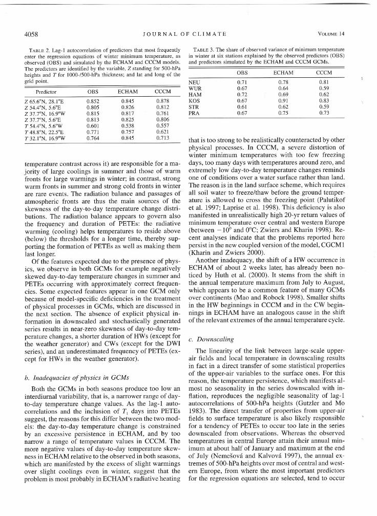
TABLE 2. Lag-I autocorrelation of predictors that most frequentlyenter the regression equations of winter minimum temperature, asobserved COBS) and simulated by the ECHAM and CCCM models.The predictors are identified by the variable, Z standing for 500-hPaheights and T for 1O00-/500-hPa thickness; and lat and long of thegrid point.

temperature contrast across it) are responsible for a ma-jority of large coolings in summer and those of warmfronts for large warmings in winter; in contrast, strongwarm fronts in summer and strong cold fronts in winterare rare events. The radiation balance and passages ofatmospheric fronts are thus the main sources of theskewness of the day-to-day temperature change distri-butions. The radiation balance appears to govern alsothe frequency and duration of PETEs: the radiativewarming (cooling) helps temperatures to reside above(below) the thresholds for a longer time, thereby sup-porting the formation of PETEs as well as making themlast longer.

Of the features expected due to the presence of phys-ics, we observe in both GCMs for example negativelyskewed day-to-day temperature changes in summer andPETEs occurring with approximately correct frequen-cies. Some expected features appear in one GCM onlybecause of model-specific deficiencies in the treatmentof physical processes in GCMs, which are discussed inthe next section. The absence of explicit physical in-formation in downscaled and stochastically generatedseries results in near-zero skewness of day-to-day tem-perature changes, a shorter duration of HWs (except forthe weather generator) and CWs (except for the DWIseries), and an underestimated frequency of PETEs (ex-cept for HWs in the weather generator).

b. Inadequacies of physics in GCMs

Both the GCMs in both seasons produce too Iowaninterdiurnal variability, that is, a narrower range of day-to-day temperature change values. As the lag-l auto-correlations and the inclusion of Tj days into PETEssuggest, the reasons for this differ between the two mod-els: the day-to-day temperature change is constrainedby an excessive persistence in ECHAM, and by toonarrow a range of temperature values in CCCM. Themore negative values of day-to-day temperature skew-ness in ECHAM relative to the observed in both seasons,which are manifested by the excess of slight warmingsover slight coolings even in winter, suggest that theproblem is most probably in ECHAM's radiative heating

TABLE 3. The share of observed variance of minimum temperaturein winter at six stations explained by the observed predictors COBS)and predictors simulated by the ECHAM and CCCM GCMs.

that is too strong to be realistically counteracted by otherphysical processes. In CCCM, a severe distortion ofwinter minimum temperatures with too few freezingdays, too many days with temperatures around zero, andextremely low day-to-day temperature changes remindsone of conditions over a water surface rather than land.The reason is in the land surface scheme, which requiresall soil water to freeze/thaw before the ground temper-ature is allowed to cross the freezing point (Palutikofet al. 1997; Laprise et al. 1998). This deficiency is alsomanifested in unrealistically high 20-yr return values ofminimum temperature over central and western Europe(between -10° and O°C;Zwiers and Kharin 1998). Re-cent analyses indicate that the problems reported herepersist in the new coupled version ofthe model, CGCMl(Kharin and Zwiers 2000).

Another inadequacy, the shift of a HW occurrence inECHAM of about 2 weeks later, has already been no-ticed by Huth et al. (2000). It stems from the shift inthe annual temperature maximum from July to August,which appears to be a common feature of many GCMsover continents (Mao and Robock 1998). Smaller shiftsin the HW beginnings in CCCM and in the CW begin-nings in ECHAM have an analogous cause in the shiftof the relevant extremes of the annual temperature cycle.

c. Downscaling

The linearity of the link between large-scale upper-air fields and local temperature in downscaling resultsin fact in a direct transfer of some statistical propertiesof the upper-air variables to the surface ones. For thisreason, the temperature persistence, which manifests al-most no seasonality in the series downscaled with in-flation, reproduces the negligible seasonality of lag-lautocorrelations of 500-hPa heights (Gutzler and Mo1983). The direct transfer of properties from upper-airfields to surface temperature is also likely responsiblefor a tendency of PETEs to occur too late in the seriesdownscaled from observations. Whereas the observedtemperatures in central Europe attain their annual min-imum at about half of January and maximum at the endof July (Nemesova and Kalvova 1997), the annual ex-tremes of 500-hPa heights over most of central and west-ern Europe, from where the most important predictorsfor the regression equations are selected, tend to occur

..

Predictor OBS ECHAM CCCM

Z 65.6°N, 28.loE 0.852 0.845 0.878Z 54.4°N, 5.6°E 0.805 0.826 0.812Z 37.7°N, 16.9°W 0.815 0.817 0.761Z 37.7°N, 5.6°E 0.813 0.825 0.806T 54.4°N, 5.6°W 0.601 0.538 0.557T 48.8°N, 22.5°E 0.771 0.757 0.621T 32.loN, 16.9°W 0.764 0.845 0.713

OBS ECHAM CCCM

NEU 0.71 0.78 0.81WUR 0.67 0.64 0.59HAM 0.72 0.69 0.62KOS 0.67 0.91 0.83STR 0.61 0.62 0.59PRA 0.67 0.75 0.73


later, in the beginning of February and August (Volmeret al. 1984).

Another issue to discuss in connection with down-scaling is the failure of the downscaling from bothGCMs in reproducing interdiurnal temperature vari-ability in winter at Neuchiitel, Kostelnf Myslova, andPrague where the DWE and DWC minimum tempera-tures have a very low lag-l autocorrelation and an over-estimated standard deviation of the day-to-day temper-ature change. The error is not regionalized: StniZnicebehaves in a different way than the two close stations(Kostelnf Myslova aJidPrague) but similarly to two dis-tant stations (Hamburg and Wtirzburg, Germany). Thesource of the error is not in the procedure of enhancingthe variance to fit the observed one, since it does notaffect persistence; and it is not in the selection of pre-dictors either, since there is no apparent difference be-tween the stations affected and those unaffected by theerror in the predictors selected and in their importancefor the regression model. Moreover, the day-to-day var-iability of 500-hPa heights and 1O00-/500-hPathicknessis reproduced quite accurately by both GCMs (Table 2),so the error does not stem from an incorrect reproductionof the time structure of predictors. The error appears tobe connected with the degree to which the observedtemperature variance is explained by the simulated pre-dictors, that is, with the factor by which the downscaledseries are multiplied to fit the observed variance. Table3 (third and fourth columns) shows that the better thesimulated circulation approximates the observed vari-ance, the worse the time structure of the downscaledseries. Two facts are worth noting in this context: first,the sites where a large share of observed temperaturevariance is explained by the simulated predictors are thesame for both GCMs; and second, the share of observedvariance explained by the observed predictors is dis-tributed among stations in a different way (see the sec-ond column in Table 3), varying from site to site muchless widely. The error, therefore, appears to be concealedin the transfer of information from simulated large-scalefields, which, for some unclear reason, fails at some ofthe stations but succeeds at the others. The problem maybe in the inconsistency that the observed regressionequations are applied to the simulated large-scale fields.

Let us turn to the effect of how the unexplained var-iance in downscaling is treated. The white noise additionleads to an unrealistically low persistence. The error islarger for winter minimum temperatures than for sum-mer maxima because large-scale predictors explain lesstemperature variance in winter, and the added noise istherefore stronger. The excessive variability of theDWW series results in the inability of temperatures toreside above (below) the thresholds for a long enoughtime. As a consequence, the number of PETEs is ex-tremely low in the DWW series, and if they occur theyare too short. Moreover, only a very small portion ofTJ days are chained to form PETEs, that is, the majorityof thermally extreme days are isolated. The white noise

addition is not the only way to enhance the variance;indeed, but any more realistic treatment of the missingvariance than the inflation is, which would consist inadding a stochastic process independent of large-scaleforcing, necessarily implies an increase in day-to-dayvariability. Our analysis shows that this would impairthe simulation of PETEs relative to the inflation ap-proach, which itself is not much successful in this re-spect. Although the physical grounds of the varianceinflation are flawed, we recommend the inflation as theleast biased approach to be used in downscaling studieswhere the time structure and prolonged extreme eventsare important.

d. Weather generator

The lag-l autocorrelations of stochastically generatedseries are too low in both seasons. This seems to be incontradiction with the fact that autocorrelations areamong the generator's parameters and should, therefore,have been replicated accurately. The explanation is asfollows. In calculating the parameters of the generator,the correlations and autocorrelations of both TMAX andTMIN are derived from the series that were normalizedseparately for wet and dry days. During the generationprocess, the generator produces normalized anomaliesfirst, which are then turned into a temperature scale bymultiplying by the standard deviations and adding tothe means, both conditioned on the precipitation oc-currence. The day-to-day changes of generated temper-atures are thus a result of superposition of the first-orderautoregressive model of normalized temperature and thefirst-order Markov chain of precipitation occurrence,which implies a suppression of lag-l autocorrelationsrelative to the original autoregressive model. Moreover,the first-order Markov chain underestimates the persis-tence of the precipitation occurrence series (Dubrovsky1997). Both effects lead to the enhancement of the day-to-day variability and underestimation of persistence inthe generated (both WGA and WGN) temperature se-nes.

The difference in performance between the WGN andWGA series can be understood from the annual cyclesof the lag-l correlations of maximum and minimumtemperatures (Fig. 1). The correlations attain their max-ima in winter and minima in summer. This makes theday-to-day temperature variability in winter lower andpersistence higher in the series where the annual cycleoflag-l correlations is implemented (WGA), relative tothat using the annual mean of lag-l correlations (WGN);the opposite holds in summer, exactly as shown in Figs.3 and 4. Since the temperature persistence is underes-timated by the weather generator in general and theannual cycle of correlations does not influence thesource of the underestimation, its inclusion acts to sup-press this bias in winter, but to enhance it in summer.In accordance with a general effect of persistence onPETEs, the inclusion of annual cycle of lag-l correla-


tions makes HWs shorter, they reach higher tempera-tures, and a lower fraction of TJ days is included inthem. On the contrary, CWs in the WGA series arelonger and more frequent relative to WGN, and higherfraction of TJ days is included in them. We can statethat the effect of inclusion of annual cycle of lag-lautocorrelations into the weather generator leads to theimprovement of several temperature and PETE statisticsin winter, but, rather paradoxically, to the deteriorationof the same characteristics in summer.

6. Conclusions

In this paper, three approaches to constructing site-specific daily temperature series, namely, the directGCM output, statistical downscaling, and the weathergenerator, were examined for their ability to reproducethe temporal structure of the series and prolonged ex-treme temperature events (PETEs). The simulated serieshave been compared against observations at six sites incentral Europe. We have arrived at the following majorconclusions.

. None of the methods of constructing site-specific dailytemperature series appears to be able to reproduce themajority of statistics of day-to-day temperaturechange and PETEs correctly. Nevertheless, theECHAM GCM output adjusted for the observed meanand variance approaches the demands most closely inwinter, whereas in summer, the weather generatorwithout the annual cycle of correlations appears toperform best.. The causes of an incorrect reproduction of the ex-amined temperature characteristics include (i) the ab-sence of physical processes, particularly surface ra-diation balance and atmospheric fronts, in the down-scaling and weather generator approach; (ii) inade-quacies in treatment of some physical processes in theGCMs; (iii) the linearity of downscaling, imposing adirect transfer of properties of large-scale fields usedas predictors to the surface temperature series; and(iv) a conjunction of the autoregressive model andMarkov chain in the generation process of maximumand minimum temperature by the weather generatortogether with an underestimation of precipitation per-sistence by the first-order Markov chain implementedin it.. The white noise addition, which is an alternative ap-proach to the variance inflation in adjusting the var-iance in downscaled series, leads to temperature seriesthat are too variable. It is therefore unsuitable if oneis concerned with time structure and prolonged ex-treme events. Although the inflation is a physicallyquestionable concept, it yields temperature time seriesmuch closer to reality.. The inclusion of the annual cycle of lag-O and lag-lcorrelations into the generator does not lead to anoverall improvement in the simulation of day-to-day

temperature variability. The reason is a general un-derestimation of persistence by the weather generator:whereas in winter the inclusion of annual cycle ofautocorrelations enhances the persistence, thereby im-proving its reproduction, in summer the inclusion ofannual cycle results in a further suppression of per-sistence, that is, in a deterioration of its reproduction.

,"

')

Acknowledgments. The authors are grateful to M.Beniston, University of Fribourg, Switzerland; A. Kast-ner, German Weather Service, Offenbach, Germany; H.Osterle, Potsdam Institute of Climate Impact Studies,Potsdam, Germany; R. Schweitzer, University of Col-orado, Boulder, Colorado; F. Zwiers, Canadian Centrefor Climate Modelling and Analysis, Victoria, Canada;and the staff of the Czech Hydrometeorological Institutein Prague, Czech Republic, for preparing and providingthe datasets. The study was supported by the GrantAgency of the Czech Republic under Projects 205/96/1670, 205/97/PI59, and 205/99/1561.

REFERENCES

Buishand, T. A., and J. J. Beersma, 1993: Jackknife tests for differ-ences in autocorrelation between climate time series. J. Climate,

6, 2490-2495.DKRZ, 1993: The ECHAM3 Atmospheric General Circulation Mod-

el. Deutsches Klimarechenzentrum Rep. 6, Hamburg, Germany,184 pp.

Domonkos, P, 1998: Statistical characteristics of extreme temperatureanomaly groups in Hungary. Theor. Appl. Climatol., 59, 165-179.

Dubrovsky, M., 1997: Creating daily weather series with use of theweather generator. Environmetrics, 8, 409-424.

-, Z. Zalud, and M. St'astna, 2000: Sensitivity of CERES-Maize

yields to statistical structure of daily weather series. ClimaticChange, 46, 447-472.

Giorgi, P, and L. O. Mearns, 1991: Approaches to the simulation ofregional climate change: A review. Rev. Geophys., 29, 191-216.

Gutzler, D. S., and K. C. Mo, 1983: Autocorrelation of Northern

Hemisphere geopotential heights. Mon. Wea. Rev., 111, 155-164.

Hay, L. E., R. L. Wilby, and G. H. Leavesley, 2000: A comparisonof delta change and downscaling GCM scenarios for three moun-tainous basins in the United States. J. Amer. Water Resour. As-

soc., 36, 387-397.Hayhoe, H. N., 2000: Improvements of stochastic weather data gen-

erators for diverse climates. Climate Res., 14, 75-87.Hulme, M., Z. C. Zhao, and T. Jiang, 1994: Recent and future climate

change in East Asia. Int. J. Climatol., 14, 637-658.Huth, R., 1999: Statistical downscaling in central Europe: Evaluation

of methods and potential predictors. Climate Res., 13, 91-101.-, and J. Kysely, 2000: Constructing site-specific climate change

scenarios on a monthly scale using statistical downscaling.Theor. Appl. Climatol., 66, 13-27.

-, -, and L. Pokorna, 2000: A GCM simulation of heat waves,dry spells, and their relationships to circulation. ClimaticChange, 46, 29-60.

Kalnay, E., and Coauthors, 1996: The NCEP/NCAR 40-Year Re-analysis Project. Bull. Amer. Meteor. Soc., 77,437-471.

Kalvova, J., and I. Nemesova, 1998: Estimating autocorrelations ofdaily extreme temperatures in observed and simulated climates.Theor. Appl. Climatol.. 59, 151-164.

-, A. Raidl, A. Trojakova, M. Zak, and I. NemeSova, 2000: Ca-nadian Climate Model-Air temperature over the European re-

~

J


..

gion and in the Czech Republic (in Czech). Meteor. Zprdvy, 53,137-145.

Karl, T. R., and R. W. Knight, 1997: The 1995 Chicago heat wave:How likely is a recurrence? Bull. Amer. Meteor. Soc., 78, 1107-1119.

-, W. C. Wang, M. E. Schlesinger, R. W. Knight, and D. Portman,1990: A method of relating general circulation model simulatedclimate to the observed local climate. Part I: Seasonal statistics.

J. Climate, 3, 1053-1079.Kattenberg, A., and Coauthors, 1996: Climate models-Projections

of future climate. Climate Change 1995: The Science of ClimateChange, J. T. Houghton et aI., Eds., Cambridge University Press,285-357.

Kharin, V. v., and F. W. Zwiers, 2000: Changes in the extremes inan ensemble of transient climate simulations with a coupledatmosphere-ocean GCM. J. Climate, 13, 3760-3788.

Kidson, J. w., and C. S. Thompson, 1998: A comparison of statisticaland model-based down scaling techniques for estimating localclimate variations. J. Climate, 11,735-753.

Laprise, R., D. Caya, M. Giguere, G. Bergeron, H. Cote, J.-P. Blan-chet, G. J. Boer, and N. A. McFarlane, 1998: Climate and climatechange in western Canada as simulated by the Canadian RegionalClimate Model. Atmos.-Ocean, 36, 119-167.

Macchiato, M., C. Serio, V. Lapenna, and L. La Rotonda, 1993:Parametric time series analysis of cold and hot spells in dailytemperature: An application in southern Italy. J. Appl. Meteor.,32, 1270-1281.

Mao, J., and A. Roback, 1998: Surface air temperature simulationsby AMIP general circulation models: Volcanic and ENSO signalsand systematic errors. J. Climate, 11, 1538-1552.

McFarlane, N. A., G. J. Boer, J.-P. Blanchet, and M. Lazare, 1992:The Canadian Climate Centre second-generation general circu-lation model and its equilibrium climate. J. Climate, 5, 1013~1044.

Mearns, L. 0., F. Giorgi, L. McDaniel, and C. Shields, 1995: Analysisof variability and diurnal range of daily temperature in a nestedregional climate model: Comparison with observations and dou-bled CO2 results. Climate Dyn., 11, 193-209.

Meehl, G. A., F. Zwiers, J. Evans, T. Knutson, L. Mearns, and P.Whetton, 2000: Trends in extreme weather and climate events:Issues related to modeling extremes in projections of future cli-mate change. Bull. Amer. Meteor. Soc., 81, 427-436.

Nemesova, I., and J. Kalvova, 1997: On the validity of ECHAM-

~

...

simulated daily extreme temperatures. Stud. Geophys. Geod., 41,396-406.

-, -, J. Buchtele, and N. Klimperova, 1998: Comparison of"GCM-simulated and observed climates for assessing hydrolog-

ical impacts of climate change. J. Hydrol. Hydromech., 46,237-263.

Palutikof, J. P., J. A. Winkler, C. M. Goodess, and J. A. Andresen,1997: The simulation of daily temperature time series from GCMoutput. Part I: Comparison of model data with observations. J.Climate, 10, 2497-2513.

Semenov, M. A., and E. M. Barrow, 1997: Use of a stochastic weathergenerator in the development of climate change scenarios. Cli-matic Change, 35, 397-414.

Skelly, W. c., and A. Henderson-Sellers, 1996: Grid box or grid point:What type of data do GCMs deliver to climate impacts research-ers? Int. J. Climatol., 16, 1079-1086.

Solow, A. R., 1988: Detecting changes through time in the varianceof a long-term hemispheric temperature record: An applicationof robust locally weighted regression. J. Climate, 1, 290-296.

Trigo, R. M., and J. P. Palutikof, 1999: Simulation of daily temper-atures for climate change scenarios over Portugal: A neural net-work model approach. Climate Res., 13, 45-59.

Volmer, J. P., M. Deque, and D. Rousselet, 1984: EOF analysis of500 mb geopotential: A comparison between simulation and re-ality. Tellus, 36A, 336-347.

von Storch, H., 1999: On the use of "inflation" in statistical down-scaling. J. Climate, 12, 3505-3506.

Wilby, R. L., L. E. Hay, and G. H. Leavesley, 1999: A comparisonof downscaled and raw GCM output: Implications for climatechange scenarios in the San Juan River basin, Colorado. J. Hy-drol., 225,67-91.

Wilks, D. S., 1992: Adapting stochastic weather generation algo-rithms for climate change studies. Climatic Change, 22, 67-84.

Winkler, J. A., J. P. Palutikof, J. A. Andresen, and C. M. Goodess,1997: The simulation of daily temperature time series from GCMoutput. Part II: Sensitivity analysis of an empirical transfer func-tion methodology. J. Climate, 10,2514-2532.

Zorita, E., and H. von Storch, 1999: The analog method as a simpledownscaling technique: Comparison with more complicatedmethods. J. Climate, 12, 2472-2489.

Zwiers, F. W., and V. V. Kharin, 1998: Changes in the extremes ofthe climate simulated by CCC GCM2 under CO2 doubling. J.Climate, 11, 2200-2222.

Time Structure of Observed, GCM-Simulated, … OCTOBER 2001 HUTH ET AL. 4047 Time Structure of Observed, GCM-Simulated, ~Downscaled, and Stochastically Generated Daily Temperature

Documents