Time step restrictions for Runge–Kutta discontinuous Galerkin methods on triangular grids

Journal of Computational Physics 227 (2008) 9697–9710

Contents lists available at ScienceDirect

Journal of Computational Physics

journal homepage: www.elsevier .com/locate / jcp

Time step restrictions for Runge–Kutta discontinuous Galerkin methodson triangular grids

Ethan J. Kubatko a,*, Clint Dawson b, Joannes J. Westerink c

a Department of Civil and Environmental Engineering and Geodetic Science, The Ohio State University, Columbus, OH 43210, United Statesb Institute for Computational Engineering and Sciences, The University of Texas at Austin, Austin, TX 78712, United Statesc Department of Civil Engineering and Geological Sciences, University of Notre Dame, Notre Dame, IN 46556, United States

a r t i c l e i n f o a b s t r a c t

Article history:Received 31 January 2008Received in revised form 18 June 2008Accepted 23 July 2008Available online 19 August 2008

Keywords:Discontinuous GalerkinStrong-stability-preservingRunge–Kutta

0021-9991/$ - see front matter � 2008 Elsevier Incdoi:10.1016/j.jcp.2008.07.026

* Corresponding author. Tel.: +1 614 292 7176.E-mail address: [email protected] (E.J. Kubatko

We derive CFL conditions for the linear stability of the so-called Runge–Kutta discontinu-ous Galerkin (RKDG) methods on triangular grids. Semidiscrete DG approximations usingpolynomials spaces of degree p ¼ 0;1;2, and 3 are considered and discretized in time usinga number of different strong-stability-preserving (SSP) Runge–Kutta time discretizationmethods. Two structured triangular grid configurations are analyzed for wave propagationin different directions. Approximate relations between the two-dimensional CFL conditionsderived here and previously established one-dimensional conditions can be observed afterdefining an appropriate triangular grid parameter h and a constant that is dependent on thepolynomial degree p of the DG spatial approximation. Numerical results verify the CFL con-ditions that are obtained, and ‘‘optimal”, in terms of computational efficiency, two-dimen-sional RKDG methods of a given order are identified.

� 2008 Elsevier Inc. All rights reserved.

1. Introduction

Runge–Kutta discontinuous Galerkin (RKDG) methods are a widely used approach for the solution of time-dependent,hyperbolic and advection dominated advection–diffusion equations – see, for example, [1,2,5–9,14,19]. The methods havebeen used to model a wide range of physical phenomena such as gas dynamics, electromagnetics, shallow water flow,and advection of contaminants. Application of RKDG methods proceeds along the classical notions of the method of lineswhereby the partial differential equation(s) (PDEs) are first discretized in space using a DG method, which produces a systemof ordinary differential equations (ODEs), and then discretized in time using a special class of explicit RK time discretizationmethods. When using explicit methods it is well known that the grid spacing and the time step Dt that are employed mustsatisfy a CFL condition in order to guarantee stability.

For RKDG methods using DG spatial discretizations of polynomials of degree p ¼ k� 1 and a k stage RK method of order k(such a method is referred to as a kth order RKDG method), Cockburn and Shu [9] give an approximate CFL condition forlinear stability of the form:

jcj DtDx6

12pþ 1

; ð1Þ

where j c j is the wave speed associated with the given problem and Dx is the uniform grid spacing. This condition is, in fact,exact for the cases p ¼ 0 and p ¼ 1 (the case p ¼ 0 can be proven trivially and the case p ¼ 1 was proven in [7]). Furthermore,

. All rights reserved.

).

9698 E.J. Kubatko et al. / Journal of Computational Physics 227 (2008) 9697–9710

for p P 2, this estimate was observed to be less than 5% smaller than numerically-obtained estimates of the CFL condition[9].

Given the somewhat restrictive nature of (1), especially as p increases, the stability of RKDG methods using so-calledstrong-stability-preserving (SSP) RK methods where the number of stages s is greater than the order k of the method wereexamined in [15] with the goal of obtaining more efficient RKDG methods. Necessary time step restrictions for stability werederived and ‘‘optimal” RKDG methods, in terms of computationally efficiency, were identified. For an RKDG method of a gi-ven order, the computational efficiency is a function of both the CFL condition and the number of stages of the SSP RK meth-od. In the majority of cases examined in [15], use of the s > k SSP RK methods was more efficient than the standard practiceof using the s ¼ k methods. This was due to gains in allowable time step size afforded by improved CFL conditions for linearstability that were large enough to offset the additional work introduced by the increased number of stages. It was found thatoptimal RKDG methods were generally obtained by using one or two additional stages than theoretically required for a givenorder.

The work cited above has been for one-dimensional RKDG methods. In recent numerical experiments, we have noted thatsimple two-dimensional analogs of these CFL conditions do not appear to be sufficient for stability in two-dimensions onstructured triangular grids. Therefore, in this paper, we seek to extend the types of one-dimensional analyses performedin [7,9,15] to RKDG methods in two-dimensions. Specifically, we derive necessary time step restrictions, which also appearto be sufficient, for the stability of RKDG methods on structured triangular grids applied to the constant coefficient, two-dimensional transport equation with periodic boundary conditions. Two different structured triangular grid patterns areexamined on which we consider wave propagation in different directions. For these grids, the stability of RKDG methodsof order k ¼ 1;2;3, and 4 are considered. In the case of the first-order RKDG method, which is equivalent to a first-order finitevolume method, CFL conditions are derived analytically by first constructing the semidiscrete DG equations over a repeatinggrid generation pattern, explicitly computing the eigenvalues of the resulting matrices, and then calculating the necessaryrestrictions so that, when scaled by the time step Dt, these eigenvalues lie within the stability region of a given RK method.For the first-order RKDG method, an exact relationship between the one- and two-dimensional CFL conditions is found oncean appropriate triangular grid spacing parameter h is defined. For the higher-order methods, we use a semi-analytical ap-proach in which the discrete equations are explicitly constructed as before but with the eigenvalues of the resulting matricesbeing computed numerically and then checked for the stability condition at a discrete number of points. In the high-ordercases, approximate relationships between the one- and two-dimensional CFL conditions can be observed using the previ-ously defined grid parameter h and a constant that is dependent on the polynomial degree p of the DG spatial discretization.The validity of these derived CFL conditions are demonstrated on numerical examples.

This paper is outlined as follows: First, in Section 2, we give a brief overview of the DG spatial discretization of the linear,two-dimensional transport equation using triangular elements, and we present the two structured, triangular grid patternsthat will be considered in our stability analysis. Next, in Section 3, we review some aspects of RK time stepping methods thatare pertinent to our objective of deriving CFL conditions. We begin by presenting the general form of the RK methods that areused and the so-called SSP theorem in Section 3.1 – noting some important facts related to this theorem that are specific tothe application of SSP RK methods to the semidiscrete DG equations. This is followed by a brief overview of the stability of RKmethods in Section 3.2. We then derive CFL conditions for RKDG methods using polynomials spaces of degree p ¼ 0;1;2, and3 and ‘‘matching order” SSP RK methods in Section 4. Several different SSP RK methods are examined, ranging from two toeight stages, and ‘‘optimal” two-dimensional RKDG methods, in terms of computational efficiency, are identified for a givenorder. This is followed by a brief subsection in which approximate relationships between the one- and two-dimensionalRKDG CFL conditions are established. Finally, in Section 5, numerical results are presented that verify our stability analysis.

2. The discontinuous Galerkin spatial discretization

In this section, we consider the DG spatial discretization of the transient, two-dimensional, linear conservation law ortransport equation over a domain X � R2 with periodic boundary conditions:

ouotþr � cu ¼ 0 in X� ð0; T� ð2Þ

uðx; y; 0Þ ¼ u0 on X;

with the vector c ¼ kckðcos h; sin hÞ (assumed to be constant) where kck and h are the magnitude and direction of wave prop-agation, respectively, and u0 is an initial condition.

Partitioning the domain X into a set of elements XE, a weak formulation of the problem is obtained by multiplying Eq. (2)by a sufficiently smooth test function v and integrating by parts over each element:

XE

ouot

vdX�Z

XE

rv � cdXþZ

CE

uc � nvds ¼ 0;

where n denotes the outward unit normal vector of CE the boundary of XE.Applying a DG method, the true solution u is approximated by uh 2 Uh and the test function v is chosen such that

v ¼ vh 2 Uh where Uh is the space PkðXEÞ of polynomials of degree k defined on XE. Due to the fact that C0 continuity is

E.J. Kubatko et al. / Journal of Computational Physics 227 (2008) 9697–9710 9699

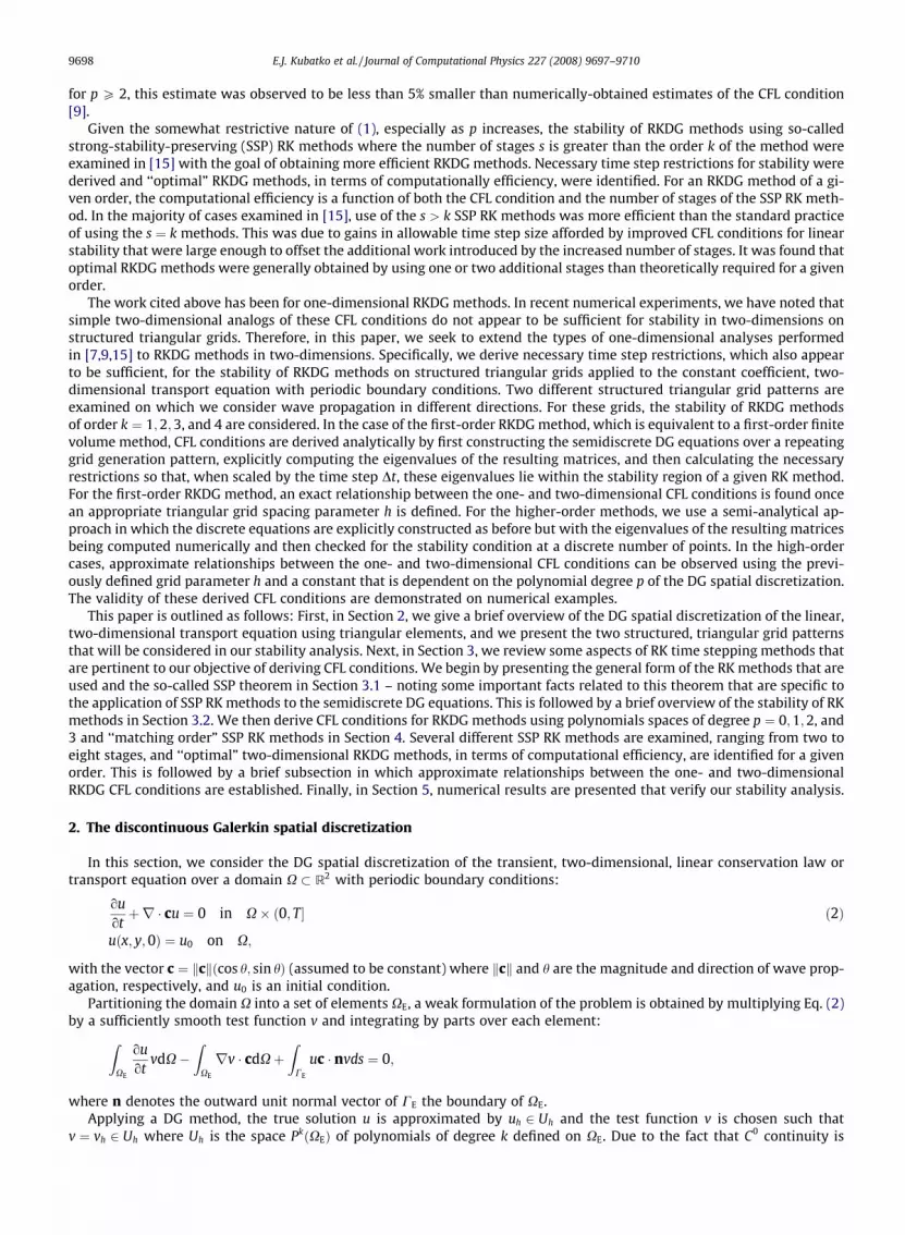
not enforced between elements in the DG method, the flux f ¼ uc � n along the boundaries CE must be approximated by anumerical flux f , which in the present case can be defined by upwinding:

f ¼u�h ðc � neÞ if c � ne P 0uþh ðc � neÞ if c � ne < 0;

(

Thus, the discrete weak form of the problem takes the following form:

ouh

otvhdX�

ZXE

rvh � cdXþZ

CE

f vhds ¼ 0:

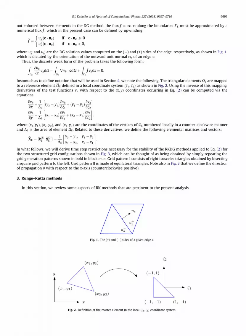
Insomuch as to define notation that will be used in Section 4, we note the following. The triangular elements XE are mappedto a reference element bXE defined in a local coordinate system ðn1; n2Þ as shown in Fig. 2. Using the inverse of this mapping,derivatives of the test functions vh with respect to the ðx; yÞ coordinates occurring in Eq. (2) can be computed via theequations:

ovh

ox¼ 1

DEðy3 � y1Þ

ovh

on1þ ðy1 � y2Þ

ovh

on2

� �ovh

oy¼ 1

DEðx1 � x3Þ

ovh

on1þ ðx2 � x1Þ

ovh

on2

� �;

where ðx1; y1Þ, ðx2; y2Þ, and ðx3; y3Þ are the coordinates of the vertices of XE numbered locally in a counter-clockwise mannerand DE is the area of element XE. Related to these derivatives, we define the following elemental matrices and vectors:

bXE ¼ ½xð1ÞE ; xð2ÞE � ¼1DE

y3 � y1; y1 � y2

x1 � x3; x2 � x1

� �:

In what follows, we will derive time step restrictions necessary for the stability of the RKDG methods applied to Eq. (2) forthe two structured grid configurations shown in Fig. 3, which can be thought of as being obtained by simply repeating thegrid generation patterns shown in bold in block m, n. Grid pattern I consists of right isosceles triangles obtained by bisectinga square grid pattern to the left. Grid pattern II is made of equilateral triangles. Note also in Fig. 3 that we define the directionof propagation h with respect to the x-axis (counterclockwise positive).

3. Runge–Kutta methods

In this section, we review some aspects of RK methods that are pertinent to the present analysis.

Fig. 1. The (+) and (�) sides of a given edge e.

Fig. 2. Definition of the master element in the local ðf1; f2Þ coordinate system.

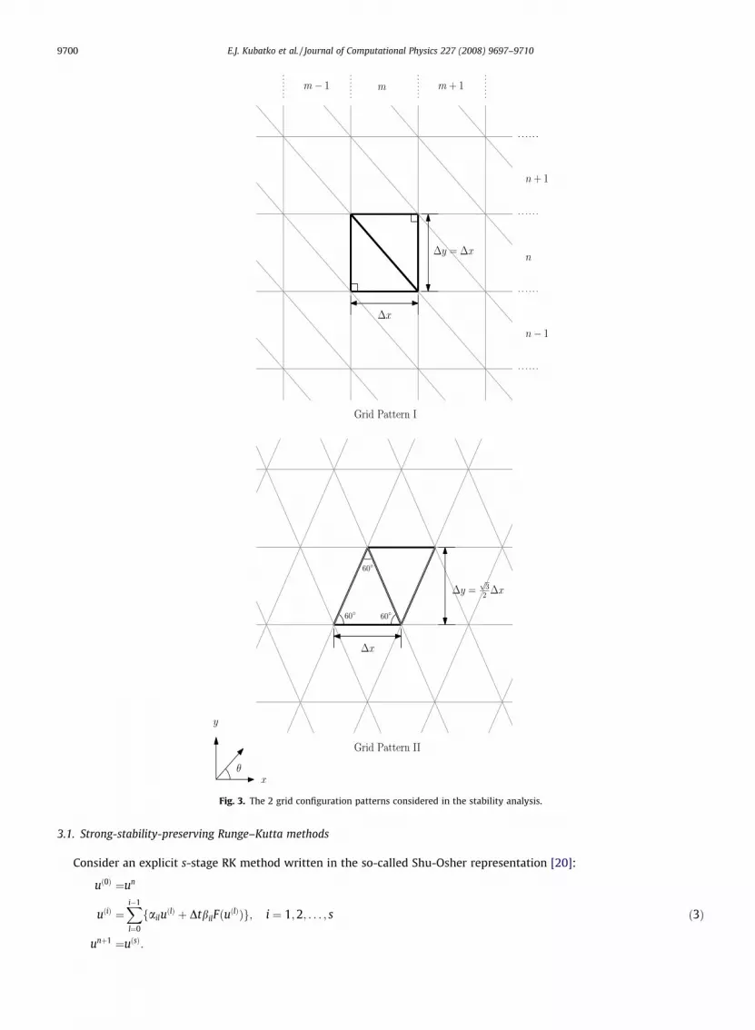
Fig. 3. The 2 grid configuration patterns considered in the stability analysis.

9700 E.J. Kubatko et al. / Journal of Computational Physics 227 (2008) 9697–9710

3.1. Strong-stability-preserving Runge–Kutta methods

Consider an explicit s-stage RK method written in the so-called Shu-Osher representation [20]:

uð0Þ ¼un

uðiÞ ¼Xi�1

l¼0

failuðlÞ þ DtbilFðuðlÞÞg; i ¼ 1;2; . . . ; s ð3Þ

unþ1 ¼uðsÞ:

E.J. Kubatko et al. / Journal of Computational Physics 227 (2008) 9697–9710 9701

If, in addition to the constraints placed on ail and bil relating to order (see, for example, [3]) and consistencyðPi�1

l¼0ail ¼ 1; i ¼ 1;2; . . . ; sÞ, the following additional constraints are enforced:

ðiÞail P 0 and bil P 0ðiiÞail ¼ 0 only if bil ¼ 0; ð4Þ

then the RK method can be written as a convex combination of forward Euler steps with time step sizes bilail

Dt, i.e.:

uð0Þ ¼un

uðiÞ ¼Xi�1

l¼0

ail uðlÞ þ Dtbil

ailFðuðlÞÞ

� �; i ¼ 1;2; . . . ; s

unþ1 ¼uðsÞ:

Such a RK method is referred to as a strong-stability-preserving (SSP) RK method, the name being based on the followingtheorem (see, for example, [13]):

Theorem 1 (The SSP Theorem). If the forward Euler method applied to the spatial discretization F is (strongly) stable in a givennorm or semi-norm under the CFL condition Dt 6 DtFE then the Runge–Kutta method (3) with constraints (4) preserves thatstability under the CFL condition:

Dt 6 jDtFE; ð5Þ

where j �mini;lðailbilÞ with ail

bil� 1 for bil ¼ 0.

Much of the research in the area of SSP methods has focused on finding optimal SSP RK methods – that is, the SSP RKmethod (5) for which j is a maximum under the given constraints placed on the ail and bil, see, for example, [18].

It is interesting to note, however, that the SSP Theorem does not provide the criteria for linear (L2) stability of the SSP RKmethods applied to semidiscrete p ¼ k� 1 DG approximations with k P 2, due to the fact that for these cases the forwardEuler method applied to the semidiscrete equations is unconditionally-unstable for a fixed Courant number m � cDt=Dx. Thiswas proven explicitly for the case k ¼ 2 in [4], and the result carries over to all p ¼ k� 1 DG spatial discretizations for k P 2[7]. Thus, in order to establish necessary time step restrictions for the linear stability of the RKDG methods the complete RKmethod must be analyzed. This is discussed in more detail in the next subsection.

The condition given in Theorem 1 does, however, play a role in the establishing the time step criteria necessary for theTVD (or TVB) property of the RKDG method (and also the linear stability of the k ¼ 1 RKDG case), since to establish the TVD(TVB) property of the RKDG methods a slope limiter is applied that renders the forward Euler method TV-stable under anappropriate CFL condition (see, for example, [9]). In two-dimensions, where enforcing the TVD property is incompatible withhigher-order accuracy [11], a slope limiter can be applied to enforce a maximum principle when using the forward Eulermethod. The timestep restriction for TV-stability or enforcement of a maximum principle for a given SSP RK method is thenprovided by condition (5). However, in general, these conditions are much weaker than those required for linear stability,and, as pointed out in [9] and as demonstrated numerically in [15], it is the linear stability condition that must be respectedor the high-order accuracy of the methods will degenerate to first-order. This fact prompted the investigation of the class ofstage-exceeding-order (i.e. s > k) SSP RK methods applied to the semidiscrete DG equations presented in [15] in order todetermine one-dimensional RKDG methods that are optimal in terms of computational efficiency, which is function of boththe CFL conditions for linear stability and the number of stages of a given RK method. In all the cases examined in that work,optimal RKDG methods were obtained using RK methods with one or more additional stages than the order of the method.For this reason, the s > k RK methods are also examined here in the two-dimensional setting.

3.2. The stability of Runge–Kutta methods

Associated with each s-stage, kth order RK method is a so-called characteristic polynomial Ps;k obtained by applying thegiven RK method to the prototypical, scalar equation _u ¼ ku where k 2 C, which can be written in the formunþ1 ¼ Ps;kðz ¼ DtkÞun. For example, the classic 2-stage, 2nd-order RK method (or modified Euler method) written in theShu-Osher representation applied to this equation gives:

uð1Þ ¼un þ zun

unþ1 ¼12

un þ 12

uð1Þ þ 12

zuð1Þ:

Substituting uð1Þ into the equation for uðnþ1Þ and simplifying gives:

unþ1 ¼ 1þ zþ 12

z2� �|fflfflfflfflfflfflfflfflfflfflfflffl{zfflfflfflfflfflfflfflfflfflfflfflffl}un

P2;2ðzÞ

:

Thus, linear stability of the RK method is guaranteed provided:

9702 E.J. Kubatko et al. / Journal of Computational Physics 227 (2008) 9697–9710

jPs;kðzÞj 6 1; ð6Þ

where j � j is the complex modulus jxþ iyj ¼ffiffiffiffiffiffiffiffiffiffiffiffiffiffiffix2 þ y2

p(x and y are real numbers and i ¼

ffiffiffiffiffiffiffi�1p

). The set in the complex planefor which condition (6) is satisfied is the so-called region of absolute stability S of the given Runge–Kutta method, that is:

S ¼ fz : jPs;kðzÞj 6 1jg:

In terms of S then, condition (6) can be written as:

Dtk � S: ð7Þ

In Fig. 4, we plot the regions of absolute stability for several of the SSP RK methods considered here where we have used thenotation SSP (s,k) to denote an s stage, kth order SSP RK method.

In the case of applying an RK method to a system of equations, i.e. when the scalar k in the equation considered above isreplaced by a matrix Lh, the issue of stability is a more delicate issue. If the matrix Lh is normal (see, for example, [22]) thenstability is guaranteed if condition (7) holds for each eigenvalue k of Lh. In the general case, however, condition (7) is only anecessary, and not a sufficient, condition for stability. Necessary and sufficient conditions in the general (non-normal) casecan be expressed in terms of the pseudospectra of Lh, see, for example, [16]. Here, with the exception of the k ¼ 1 RKDG case,we will content ourselves with finding necessary conditions according to (7). These conditions also appear to be sufficient aswill be demonstrated in the numerical results section.

Fig. 4. Regions of absolute stability for the various SSP (s,k) RK methods.

E.J. Kubatko et al. / Journal of Computational Physics 227 (2008) 9697–9710 9703

4. Stability analysis

The discrete equations for the grid generation patterns shown in Fig. 3 can be written in the following compactform:

Mddt

Um;n ¼ AUm;n � BUm1;n � CUm;n1; ð8Þ

where Um;n is a vector containing the degrees of freedom for both of the elements in the grid block m;n (refer to Fig. 3), i.e.:

Um;n ¼u1

u2

� �:

Here u1 and u2 are vectors of length Nd containing the degrees of freedom of elements 1 and 2, respectively, of the given gridconfiguration (Nd ¼ ðpþ 1Þðpþ 2Þ=2 for a degree p triangular element). The mass matrix M is block diagonal:

M ¼m1 00 m2

� �;

with blocks mE, the elemental mass matrices, given by:

mE ¼DE

2m; mij ¼

ZbXE

/i/jdbXE;

where mij is the ijth entry of the matrix m.The matrix A is made up of both elemental and edge contributions:

A ¼ bAE þ eAe:

The matrix bAE, like the mass matrix, is block diagonal with the blocks given by:

aE ¼X2

k¼1

ðc � xðkÞE ÞaðkÞ; aðkÞij ¼ZbXe

o/i

onk/jdbXE:

The matrix eAe corresponds to contributions from the edge integrals that are interior to the grid generation pattern and theoutflow edges on the boundary of the grid generation pattern. It is made up of blocks ~ae:

~ae ¼l2ðc � nÞ~a; ~aij ¼

Ze

/i/jds:

The matrices B and C are made up of the same blocks ~ae, but corresponding to edges that are inflow edges on the boundary ofthe grid generation pattern. The structure of these matrices changes based on the wave propagation direction h, which dic-tates the upwind direction. For example, the matrices of grid pattern I for 0 6 h 6 p=2 and grid pattern II for 0 6 h 6 p=3 willhave the following structures:

eAe ¼X; 0X; X þ X

� �; B� ¼

0; X

0; 0

� �; C� ¼

0; X

0; 0

� �;

where the X’s correspond to the matrices ~ae of a particular edge.Following the ideas of classic Von Neumann stability analysis (see, for example, [17]), we seek a solution in the following

form:

Um;n ¼ bUm;neiðkxmDxþkynDyÞ;

where kx and ky are wave numbers associated with the x and y directions, respectively. Substituting this into Eq. (8) andinverting the mass matrix, the following equation is obtained:

ddtbUm;n ¼ Lh

bUm;n;

where the matrix Lh, the DG spatial operator, is defined as:

Lh �M�1ðA� BeikxmDx � CeikynDyÞ:

4.1. First-order RKDG method (k ¼ 1)

The first-order RKDG method, which uses piecewise constants for the DG spatial discretization and the first-order forwardEuler method in time, can be examined analytically. As an example, we consider the problem of propagation in the range0 6 h 6 p=2 on the first grid pattern. For this case, the matrix Lh is given by:

9704 E.J. Kubatko et al. / Journal of Computational Physics 227 (2008) 9697–9710

Lh ¼ 2kck 1Dx

cos h�1 e�ia

1 �1

" #þ sin h

�1 e�ib

1 �1

" #( );

where a � kxmDx, b � kynDy 2 ½0;2p� (note Dx ¼ Dy for grid pattern I). It is a simple matter to verify that this is a normalmatrix so condition (7) is necessary and sufficient for stability. We explicitly compute the eigenvalues of Lh:

k ¼ �2kck 1Dx

HffiffiffiffiffiffiffiffiffiffiffiffiffiffiffiffiffiffiffiffiffiffiffiffiffiffiffiHðHc � iHsÞ

q� �;

where

H � cos hþ sin h

Hc � cos h cos aþ sin h cos b

Hs � cos h sin aþ sin h sin b:

The stability condition (6) must be satisified for z ¼ Dtk. The characteristic polynomial of the forward Euler method is sim-ply P1;1 ¼ 1þ z and so, in this case, assuming the separation of k into real Re and imaginary Im parts, condition (6) reads:

jP1;1ðzÞj2 ¼ 1þ m½2ReðKÞ þ mðReðKÞ2 þImðKÞ2Þ� 6 1; ð9Þ

where K � kDx=kck and m is the Courant number (in two-dimensions we are initially defining this as m ¼ cDt=Dx). Assum-ing that both ReðKÞ–0 and ImðKÞ–0, inequality (9) can only be satisfied for m > 0 provided:

m 6 �m � �2ReðKÞReðKÞ2 þImðKÞ2

: ð10Þ

With the help of the following identity for the square root of a complex number (see, for example, [21]):

p¼

ffiffiffi2p

2

ffiffiffiffiffiffiffiffiffiffiffiffiffiffiffiffiffiffiffiffiffiffiffiffiffiffiffiffiffiffiffiffiffiffiffiffiffiffiffiffiffiffiffix2 þ y2

pþ x

qþ isgnðyÞ

ffiffiffi2p

2

ffiffiffiffiffiffiffiffiffiffiffiffiffiffiffiffiffiffiffiffiffiffiffiffiffiffiffiffiffiffiffiffiffiffiffiffiffiffiffiffiffiffiffix2 þ y2

p� x

q;

the left side of (10) can be written in the form:

�m ¼ 12H

ReðKÞ

ReðKÞ þ ðH�ffiffiffiffiffiffiffiffiffiffiffiffiffiffiffiffiffiffiffiH2

c þH2s

qÞ

8><>:9>=>;;

where

ReðKÞ ¼ � 2Hffiffiffiffiffiffiffiffiffiffiffiffiffiffiffiffiffiffiffiffiffiffiffiffiffiffiffiffiffiffiffiffiffiffiffiffiffiffiffiffiffiffiffiffiffiffi2Hð

ffiffiffiffiffiffiffiffiffiffiffiffiffiffiffiffiffiffiffiH2

c þH2s

qþHcÞ

r" #:

It can be shown that ReðKÞ 6 0 and that 0 6 H�ffiffiffiffiffiffiffiffiffiffiffiffiffiffiffiffiffiffiffiH2

c þH2s

q6 �ReðKÞ. Thus, �m has a minimum value of 1=2H over the

range of all a and b, and the condition for stability is simply:

m 6 �m ¼ 12H

:

Recall that this expression is valid for directions of propagation 0 6 h 6 p=2 on grid pattern I, which corresponds to1 6 H 6

ffiffiffi2p

. In this range, the stability condition is most restrictive at h ¼ p=4, in which case m 6ffiffiffi2p

=4, and least restrictiveat h ¼ 0 and p=2 when the direction of propagation is along the shorter element edges, in which case m 6 1=2.

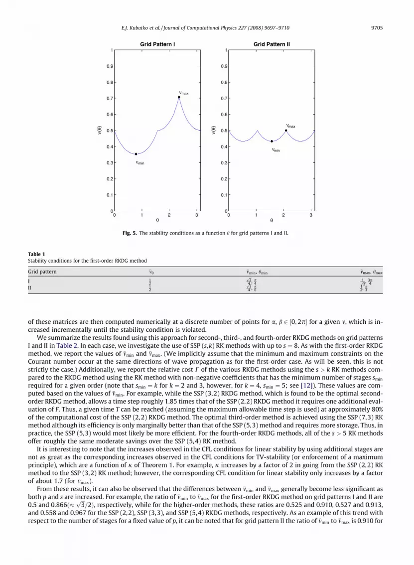
Stability conditions for the full spectrum of propagation directions for grid patterns I and II can be derived in an analogousmanner. Due to symmetry of the grids, stability conditions only need to be evaluated in the range 0 6 h < h where h ¼ p forgrid pattern I and h ¼ p=3 for grid pattern II. These conditions are plotted in Fig. 5 as functions of h. Note that for grid patternI, the stability condition in the full range of propagation is least restrictive at h ¼ 3p=4, when the direction of propagation isparallel to the longest element edge. In fact, this condition, m 6 1=

ffiffiffi2p

, corresponds to the well-known two-dimensional CFLcondition for a finite difference scheme on a rectilinear grid. We elaborate on this in Section 4.3. Similarly, for grid pattern II,the stability condition is least restrictive, in this case m 6 1=2, when the direction of propagation is parallel to the elementedges. The most restrictive conditions are m 6

ffiffiffi2p

=4 and m 6ffiffiffi3p

=4 at h ¼ p=4 and h ¼ p=6 for grid patterns I and II, respec-tively. These extremum conditions, denoted �mmin and �mmax, are summarized in Table 1 along with the condition for propaga-tion for h ¼ 0, denoted �m0. Finally, we note that the stability condition for a given RK method applied to the p ¼ 0 DG spatialdiscretization is given by the SSP theorem since for this case the forward Euler method is stable for a given Courant number.

4.2. Higher-order RKDG methods (k P 2)

In this section, we examine the higher-order RKDG cases. As in the k ¼ 1 case, we explicitly compute the form of the DGspatial operators Lh. Following the approach outlined earlier in this section, this is a straightforward process. The eigenvalues

0 1 2 30

0.1

0.2

0.3

0.4

0.5

0.6

0.7

0.8

0.9

1

θ

(θν)

(θν

ν

ν

)

Grid Pattern I

0 1 2 30

0.1

0.2

0.3

0.4

0.5

0.6

0.7

0.8

0.9

1

θ

Grid Pattern II

min

max

min

max

ν

ν

Fig. 5. The stability conditions as a function h for grid patterns I and II.

Table 1Stability conditions for the first-order RKDG method

Grid pattern �m0 �mmin, hmin �mmax, hmax

I 12

ffiffi2p

4 , p4

1ffiffi2p , 3p

4II 1

2

ffiffi3p

4 , p6

12, p

3

E.J. Kubatko et al. / Journal of Computational Physics 227 (2008) 9697–9710 9705

of these matrices are then computed numerically at a discrete number of points for a, b 2 ½0;2p� for a given m, which is in-creased incrementally until the stability condition is violated.

We summarize the results found using this approach for second-, third-, and fourth-order RKDG methods on grid patternsI and II in Table 2. In each case, we investigate the use of SSP (s,k) RK methods with up to s ¼ 8. As with the first-order RKDGmethod, we report the values of �mmin and �mmax. (We implicitly assume that the minimum and maximum constraints on theCourant number occur at the same directions of wave propagation as for the first-order case. As will be seen, this is notstrictly the case.) Additionally, we report the relative cost C of the various RKDG methods using the s > k RK methods com-pared to the RKDG method using the RK method with non-negative coefficients that has the minimum number of stages smin

required for a given order (note that smin ¼ k for k ¼ 2 and 3, however, for k ¼ 4, smin ¼ 5; see [12]). These values are com-puted based on the values of �mmin. For example, while the SSP (3,2) RKDG method, which is found to be the optimal second-order RKDG method, allows a time step roughly 1.85 times that of the SSP (2,2) RKDG method it requires one additional eval-uation of F. Thus, a given time T can be reached (assuming the maximum allowable time step is used) at approximately 80%of the computational cost of the SSP (2,2) RKDG method. The optimal third-order method is achieved using the SSP (7,3) RKmethod although its efficiency is only marginally better than that of the SSP (5,3) method and requires more storage. Thus, inpractice, the SSP (5,3) would most likely be more efficient. For the fourth-order RKDG methods, all of the s > 5 RK methodsoffer roughly the same moderate savings over the SSP (5,4) RK method.

It is interesting to note that the increases observed in the CFL conditions for linear stability by using additional stages arenot as great as the corresponding increases observed in the CFL conditions for TV-stability (or enforcement of a maximumprinciple), which are a function of j of Theorem 1. For example, j increases by a factor of 2 in going from the SSP (2,2) RKmethod to the SSP (3,2) RK method; however, the corresponding CFL condition for linear stability only increases by a factorof about 1.7 (for �mmax).

From these results, it can also be observed that the differences between �mmin and �mmax generally become less significant asboth p and s are increased. For example, the ratio of �mmin to �mmax for the first-order RKDG method on grid patterns I and II are0.5 and 0:866ð�

ffiffiffi3p

=2Þ, respectively, while for the higher-order methods, these ratios are 0.525 and 0.910, 0.527 and 0.913,and 0.558 and 0.967 for the SSP (2,2), SSP (3,3), and SSP (5,4) RKDG methods, respectively. As an example of this trend withrespect to the number of stages for a fixed value of p, it can be noted that for grid pattern II the ratio of �mmin to �mmax is 0.910 for

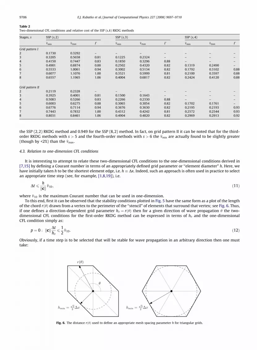
Table 2Two-dimensional CFL conditions and relative cost of the SSP (s,k) RKDG methods

Stages, s SSP (s,2) SSP (s,3) SSP (s,4)

�mmin �mmax C �mmin �mmax C �mmin �mmax C

Grid pattern I2 0.1730 0.3292 – – – – – – –3 0.3205 0.5658 0.81 0.1225 0.2324 – – – –4 0.4150 0.7447 0.83 0.1850 0.3296 0.88 – – –5 0.4901 0.8874 0.88 0.2502 0.4320 0.82 0.1319 0.2490 –6 0.5533 1.0061 0.94 0.3002 0.5134 0.82 0.1792 0.3102 0.887 0.6077 1.1076 1.00 0.3521 0.5999 0.81 0.2100 0.3597 0.888 0.6557 1.1965 1.06 0.4004 0.6817 0.82 0.2424 0.4120 0.88

Grid pattern II2 0.2119 0.2328 – – – – – – –3 0.3925 0.4001 0.81 0.1500 0.1643 – – – –4 0.5083 0.5266 0.83 0.2266 0.2330 0.88 – – –5 0.6003 0.6275 0.88 0.3065 0.3054 0.82 0.1702 0.1761 –6 0.6776 0.7114 0.94 0.3676 0.3630 0.82 0.2195 0.2193 0.937 0.7443 0.7832 1.00 0.4312 0.4242 0.81 0.2572 0.2544 0.938 0.8031 0.8461 1.06 0.4904 0.4820 0.82 0.2969 0.2913 0.92

9706 E.J. Kubatko et al. / Journal of Computational Physics 227 (2008) 9697–9710

the SSP (2,2) RKDG method and 0.949 for the SSP (8,2) method. In fact, on grid pattern II it can be noted that for the third-order RKDG methods with s > 5 and the fourth-order methods with s > 6 the �mmin are actually found to be slightly greater(though by <2%) than the �mmax.

4.3. Relation to one-dimension CFL conditions

It is interesting to attempt to relate these two-dimensional CFL conditions to the one-dimensional conditions derived in[7,15] by defining a Courant number in terms of an appropriately defined grid parameter or ‘‘element diameter” h. Here, wehave initially taken h to be the shortest element edge, i.e. h � Dx. Indeed, such an approach is often used in practice to selectan appropriate time step (see, for example, [1,8,19]), i.e.

Dt 6hkck

�m1D; ð11Þ

where �m1D is the maximum Courant number that can be used in one-dimension.To this end, first it can be observed that the stability conditions plotted in Fig. 5 have the same form as a plot of the length

of the chord rðhÞ drawn from a vertex to the perimeter of the ‘‘stencil” of elements that surround that vertex; see Fig. 6. Thus,if one defines a direction-dependent grid parameter hh ¼ rðhÞ then for a given direction of wave propagation h the two-dimensional CFL conditions for the first-order RKDG method can be expressed in terms of hh and the one-dimensionalCFL condition simply as:

p ¼ 0 : kckDthh6

12

�m1D: ð12Þ

Obviously, if a time step is to be selected that will be stable for wave propagation in an arbitrary direction then one musttake:

Fig. 6. The distance rðhÞ used to define an appropriate mesh spacing parameter h for triangular grids.

E.J. Kubatko et al. / Journal of Computational Physics 227 (2008) 9697–9710 9707

p ¼ 0 : Dt 612

hmin

kck ; ð13Þ

where hmin is the radius of the largest circle that is entirely contained within the stencil of elements surrounding a vertex (seeFig. 6) and where we have used the fact that �m1D ¼ 1 for the first-order RKDG method. We remark that this definition of hmin

has an obvious relation to the two-dimensional CFL condition for a finite difference method on a rectilinear grid – namely,that the domain of dependence of a finite difference grid point, which is a spherical cone in two-dimensions, must be con-tained within the finite difference stencil; see [10]. Note that condition (13), which is necessary and sufficient for stability, isstricter than using condition (11) with h defined as the shortest element edge or the diameter of the inscribed circle of theelement – two approaches that are commonly used in practice.

This simple result, however, does not hold for the higher-order RKDG methods. However, for the second-order RKDGmethods, it can be observed that if the factor of 1/2 of condition (12) is replaced by 1=

ffiffiffi2p

then one obtains a good approx-imation of the two-dimensional CFL conditions reported in Table 2 in terms of their one-dimensional counterparts. This leadsus to consider the general condition:

kckDthh6

1

21=ðpþ1Þ�m1D: ð14Þ

Of course, for p ¼ 0 we recover condition (11), which is an exact relation for the two-dimensional CFL conditions expressedin terms of the one-dimensional results. For p ¼ 1, the estimates provided by (14) for �mmax are generally within 2% of thosereported in Table 2 for both grid patterns I and II (the only exception being the SSP (3,2) method, which is within 4%). Forp ¼ 2 and p ¼ 3, these estimates are within 7% for grid pattern I and 5% for grid pattern II. The estimates for �mmin provided by(14) are less accurate – though they are still within 10% of the computed values, with the errors increasing with the numberof stages.

5. Numerical results

In this section, we verify the various stability conditions obtained in the previous section. We consider an initial conditiongiven by a two-dimensional Gaussian function of the form:

u0ðx; yÞ ¼A

2pre�ðx

2þy2Þ=2r2; ð15Þ

where A and r are positive constants (see Fig. 7). Periodic boundary conditions are used, and we consider the two grid con-figurations of Fig. 3 with Dy ¼ 0:08. To examine wave propagation in the directions corresponding to �mmin and �mmax for eachgrid pattern, we rotate the grid patterns and define the boundaries accordingly. For example, the conditions for �mmax areexamined using the grids shown in Fig. 8(a) and (b) by taking c ¼ ð1;0Þ in Eq. (2).

Fig. 7. The initial condition used for the numerical test.

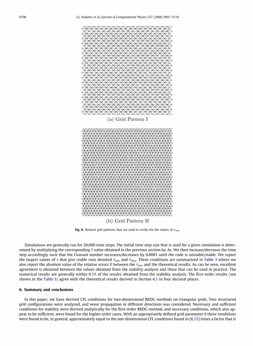
Fig. 8. Rotated grid patterns that are used to verify the the values of mmax.

9708 E.J. Kubatko et al. / Journal of Computational Physics 227 (2008) 9697–9710

Simulations are generally run for 20,000 time steps. The initial time step size that is used for a given simulation is deter-mined by multiplying the corresponding �m value obtained in the previous section by Dx. We then increase/decrease the timestep accordingly such that the Courant number increases/decreases by 0.0001 until the code is unstable/stable. We reportthe largest values of m that give stable runs denoted mmin and mmax. These conditions are summarized in Table 3 where wealso report the absolute value of the relative errors E between the mmin and the theoretical results. As can be seen, excellentagreement is obtained between the values obtained from the stability analysis and those that can be used in practice. Thenumerical results are generally within 0.1% of the results obtained from the stability analysis. The first-order results (notshown in the Table 3) agree with the theoretical results derived in Section 4.1 to four decimal places.

6. Summary and conclusions

In this paper, we have derived CFL conditions for two-dimensional RKDG methods on triangular grids. Two structuredgrid configurations were analyzed, and wave propagation in different directions was considered. Necessary and sufficientconditions for stability were derived analytically for the first-order RKDG method, and necessary conditions, which also ap-pear to be sufficient, were found for the higher-order cases. With an appropriately defined grid parameter h these conditionswere found to be, in general, approximately equal to the one-dimensional CFL conditions found in [6,15] times a factor that is

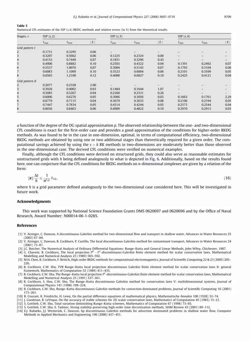
Table 3Numerical CFL estimates of the SSP (s, k) RKDG methods and relative errors (in %) from the theoretical results

Stages, s SSP (s,2) SSP (s,3) SSP (s,4)

mmin mmax j E j mmin mmax j E j mmin mmax j E j

Grid pattern I2 0.1731 0.3295 0.06 – – – – – –3 0.3207 0.5662 0.06 0.1225 0.2324 0.00 – – –4 0.4153 0.7449 0.07 0.1851 0.3296 0.43 – – –5 0.4906 0.8882 0.10 0.2503 0.4322 0.04 0.1391 0.2492 0.076 0.5537 1.0070 0.07 0.3004 0.5143 0.07 0.1793 0.3104 0.067 0.6083 1.1099 0.10 0.3523 0.6004 0.06 0.2101 0.3599 0.058 0.6565 1.2100 0.12 0.4008 0.6827 0.10 0.2425 0.4121 0.04

Grid pattern II2 0.2077 0.2328 2.00 – – – – – –3 0.3926 0.4002 0.03 0.1484 0.1644 1.07 – – –4 0.5085 0.5267 0.04 0.2260 0.2331 0.26 – – –5 0.6006 0.6276 0.05 0.3066 0.3056 0.03 0.1663 0.1761 2.296 0.6779 0.7115 0.04 0.3679 0.3633 0.08 0.2196 0.2194 0.057 0.7447 0.7834 0.05 0.4314 0.4244 0.05 0.2573 0.2544 0.048 0.8036 0.8463 0.06 0.4909 0.4822 0.10 0.2970 0.2913 0.03

E.J. Kubatko et al. / Journal of Computational Physics 227 (2008) 9697–9710 9709

a function of the degree of the DG spatial approximation p. The observed relationship between the one- and two-dimensionalCFL conditions is exact for the first-order case and provides a good approximation of the conditions for higher-order RKDGmethods. As was found to be in the case in one-dimension, optimal, in terms of computational efficiency, two-dimensionalRKDG methods are obtained by using one or two additional stages than theoretically required for a given order. The com-putational savings achieved by using the s > k RK methods in two-dimensions are moderately better than those observedin the one-dimensional case. The derived CFL conditions were verified on numerical examples.

Finally, although the CFL conditions were derived on structured grids, they could also serve as reasonable estimates forunstructured grids with h being defined analogously to what is depicted in Fig. 6. Additionally, based on the results foundhere, one can conjecture that the CFL conditions for RKDG methods on n-dimensional simplexes are given by a relation of theform:

kckDth6

1nf ðpÞ

�m1D; ð16Þ

where h is a grid parameter defined analogously to the two-dimensional case considered here. This will be investigated infuture work.

Acknowledgments

This work was supported by National Science Foundation Grants DMS 0620697 and 0620696 and by the Office of NavalResearch, Award Number: N00014-06-1-0285.

References

[1] V. Aizinger, C. Dawson, A discontinuous Galerkin method for two-dimensional flow and transport in shallow water, Advances in Water Resources 25(2002) 67–84.

[2] V. Aizinger, C. Dawson, B. Cockburn, P. Castillo, The local discontinuous Galerkin method for contaminant transport, Advances in Water Resources 24(2001) 73–87.

[3] J.C. Butcher, The Numerical Analysis of Ordinary Differential Equations: Runge–Kutta and General Linear Methods, John Wiley, Chichester, 1987.[4] G. Chavent, B. Cockburn, The local projection P0 � P1-discontinuous-Galerkin finite element method for scalar conservation laws, Mathematical

Modelling and Numerical Analysis 23 (1989) 565–592.[5] M.H. Chen, B. Cockburn, F. Reitich, High-order RKDG methods for computational electromagnetics, Journal of Scientific Computing 22 & 23 (2005) 205–

226.[6] B. Cockburn, C.W. Shu, TVB Runge–Kutta local projection discontinuous Galerkin finite element method for scalar conservation laws II: general

framework, Mathematics of Computation 52 (1989) 411–435.[7] B. Cockburn, C.W. Shu, The Runge–Kutta local projection P1-discontinuous-Galerkin finite element method for scalar conservation laws, Mathematical

Modelling and Numerical Analysis 25 (1991) 337–361.[8] B. Cockburn, S. Hou, C.W. Shu, The Runge–Kutta discontinuous Galerkin method for conservation laws V: multidimensional systems, Journal of

Computational Physics 141 (1998) 199–224.[9] B. Cockburn, C.W. Shu, Runge–Kutta discontinuous Galerkin methods for convection dominated problems, Journal of Scientific Computing 16 (2001)

173–261.[10] R. Courant, K. Friedrichs, H. Lewy, On the partial difference equations of mathematical physics, Mathematische Annalen 100 (1928) 32–74.[11] J. Goodman, R. LeVeque, On the accuracy of stable schemes for 2D scalar conservation laws, Mathematics of Computation 45 (1985) 15–21.[12] S. Gottlieb, C.W. Shu, Total variation diminishing Runge–Kutta schemes, Mathematics of Computation 67 (1998) 73–85.[13] S. Gottlieb, C.W. Shu, E. Tadmor, Strong stability-preserving high-order time discretization methods, SIAM Review 43 (2001) 89–112.[14] E.J. Kubatko, J.J. Westerink, C. Dawson, hp discontinuous Galerkin methods for advection dominated problems in shallow water flow, Computer

Methods in Applied Mechanics and Engineering 196 (2006) 437–451.

9710 E.J. Kubatko et al. / Journal of Computational Physics 227 (2008) 9697–9710

[15] E.J. Kubatko, J.J. Westerink, C. Dawson, Semidiscrete discontinuous Galerkin methods and stage-exceeding-order, strong-stability-preserving Runge–Kutta time discretizations, Journal of Computational Physics 222 (2007) 832–848.

[16] S.C. Reddy, L.N. Trefethen, Stability of the method of lines, Numerische Mathematik 62 (1992) 235–267.[17] R.D. Richtmyer, K.W. Morton, Difference Methods for Initial-Value Problems, 2nd ed., John Wiley, New York, 1967.[18] S.J. Ruuth, Global optimization of explicit strong-stability-preserving Runge–Kutta methods, Mathematics of Computation 75 (2006) 183–207.[19] D. Srmny, M.A. Botchev, J.J.W. van der Vegt, Dispersion and dissipation error in high-order Runge–Kutta discontinuous Galerkin discretisations of the

Maxwell equations, Journal of Scientific Computing 33 (2007) 47–74.[20] C.W. Shu, S. Osher, Efficient implementation of essentially non-oscillatory shock-capturing schemes, Journal of Computational Physics 77 (1988) 439–

471.[21] J. Spanier, K.B. Oldham, An Atlas of Functions, Hemisphere, Washington, DC, 1987.[22] G. Strang, Linear Algebra and its Applications, Academic Press, New York, 1970.