Time Series Scenarios - SAP · PDF filePUBLIC SAP BusinessObjects Predictive Analytics 3.1 2017-10-26 Time Series Scenarios Automated Analytics User Guide

PUBLIC

SAP BusinessObjects Predictive Analytics 3.12017-10-26

Time Series ScenariosAutomated Analytics User Guide

Content

1 Welcome to this Guide. . . . . . . . . . . . . . . . . . . . . . . . . . . . . . . . . . . . . . . . . . . . . . . . . . . . . . . . 41.1 What's New in Time Series Scenarios. . . . . . . . . . . . . . . . . . . . . . . . . . . . . . . . . . . . . . . . . . . . . . . 4

Document History. . . . . . . . . . . . . . . . . . . . . . . . . . . . . . . . . . . . . . . . . . . . . . . . . . . . . . . . . . 41.2 About this Document. . . . . . . . . . . . . . . . . . . . . . . . . . . . . . . . . . . . . . . . . . . . . . . . . . . . . . . . . . 41.3 Before Beginning. . . . . . . . . . . . . . . . . . . . . . . . . . . . . . . . . . . . . . . . . . . . . . . . . . . . . . . . . . . . . 5

Files and Documentation Provided with this Guide. . . . . . . . . . . . . . . . . . . . . . . . . . . . . . . . . . . 5Displaying the Contextual Help. . . . . . . . . . . . . . . . . . . . . . . . . . . . . . . . . . . . . . . . . . . . . . . . . 6

2 General Introduction to Scenarios. . . . . . . . . . . . . . . . . . . . . . . . . . . . . . . . . . . . . . . . . . . . . . . 72.1 Scenario 1. . . . . . . . . . . . . . . . . . . . . . . . . . . . . . . . . . . . . . . . . . . . . . . . . . . . . . . . . . . . . . . . . . 72.2 Scenario 2. . . . . . . . . . . . . . . . . . . . . . . . . . . . . . . . . . . . . . . . . . . . . . . . . . . . . . . . . . . . . . . . . . 72.3 Introduction to Sample Files. . . . . . . . . . . . . . . . . . . . . . . . . . . . . . . . . . . . . . . . . . . . . . . . . . . . . 7

Additional Sample Files. . . . . . . . . . . . . . . . . . . . . . . . . . . . . . . . . . . . . . . . . . . . . . . . . . . . . . 92.4 File Format Specifications. . . . . . . . . . . . . . . . . . . . . . . . . . . . . . . . . . . . . . . . . . . . . . . . . . . . . . . 92.5 Starting a Time Series Analysis. . . . . . . . . . . . . . . . . . . . . . . . . . . . . . . . . . . . . . . . . . . . . . . . . . 10

3 Scenario 1: Standard Modeling with Time Series. . . . . . . . . . . . . . . . . . . . . . . . . . . . . . . . . . . . 113.1 Application Options. . . . . . . . . . . . . . . . . . . . . . . . . . . . . . . . . . . . . . . . . . . . . . . . . . . . . . . . . . . 11

Printing the Screen. . . . . . . . . . . . . . . . . . . . . . . . . . . . . . . . . . . . . . . . . . . . . . . . . . . . . . . . . 11Saving the Screen Content. . . . . . . . . . . . . . . . . . . . . . . . . . . . . . . . . . . . . . . . . . . . . . . . . . . 11Copying the Screen Content. . . . . . . . . . . . . . . . . . . . . . . . . . . . . . . . . . . . . . . . . . . . . . . . . . 12

3.2 Step 1 - Defining the Modeling Parameters. . . . . . . . . . . . . . . . . . . . . . . . . . . . . . . . . . . . . . . . . . .12Selecting a Data Source. . . . . . . . . . . . . . . . . . . . . . . . . . . . . . . . . . . . . . . . . . . . . . . . . . . . . 12Selecting a Cutting Strategy. . . . . . . . . . . . . . . . . . . . . . . . . . . . . . . . . . . . . . . . . . . . . . . . . . 13Describing the Data Selected. . . . . . . . . . . . . . . . . . . . . . . . . . . . . . . . . . . . . . . . . . . . . . . . . .13Selecting Variables. . . . . . . . . . . . . . . . . . . . . . . . . . . . . . . . . . . . . . . . . . . . . . . . . . . . . . . . . 15Checking Modeling Parameters. . . . . . . . . . . . . . . . . . . . . . . . . . . . . . . . . . . . . . . . . . . . . . . . 17

3.3 Step 2 - Generating the Model. . . . . . . . . . . . . . . . . . . . . . . . . . . . . . . . . . . . . . . . . . . . . . . . . . . 21Generating the Model. . . . . . . . . . . . . . . . . . . . . . . . . . . . . . . . . . . . . . . . . . . . . . . . . . . . . . . 21Following the Progress of the Generation Process. . . . . . . . . . . . . . . . . . . . . . . . . . . . . . . . . . . 21Visualizing the Model Results. . . . . . . . . . . . . . . . . . . . . . . . . . . . . . . . . . . . . . . . . . . . . . . . . 22

3.4 Step 3 - Analyzing and Understanding the Generated Model . . . . . . . . . . . . . . . . . . . . . . . . . . . . . 23Model Debriefing. . . . . . . . . . . . . . . . . . . . . . . . . . . . . . . . . . . . . . . . . . . . . . . . . . . . . . . . . . 23Forecasts. . . . . . . . . . . . . . . . . . . . . . . . . . . . . . . . . . . . . . . . . . . . . . . . . . . . . . . . . . . . . . . 28Signal Components. . . . . . . . . . . . . . . . . . . . . . . . . . . . . . . . . . . . . . . . . . . . . . . . . . . . . . . . 31Regressions: Contribution by Variables. . . . . . . . . . . . . . . . . . . . . . . . . . . . . . . . . . . . . . . . . . 34Statistical Reports. . . . . . . . . . . . . . . . . . . . . . . . . . . . . . . . . . . . . . . . . . . . . . . . . . . . . . . . . 35

2 P U B L I CTime Series Scenarios

Content

3.5 Step 4 - Using the Model. . . . . . . . . . . . . . . . . . . . . . . . . . . . . . . . . . . . . . . . . . . . . . . . . . . . . . . 39Applying the Model. . . . . . . . . . . . . . . . . . . . . . . . . . . . . . . . . . . . . . . . . . . . . . . . . . . . . . . . 39Saving the Model. . . . . . . . . . . . . . . . . . . . . . . . . . . . . . . . . . . . . . . . . . . . . . . . . . . . . . . . . . 43Opening a Model. . . . . . . . . . . . . . . . . . . . . . . . . . . . . . . . . . . . . . . . . . . . . . . . . . . . . . . . . . 44

4 Scenario 2: Modeling with Extra Predictable Variables. . . . . . . . . . . . . . . . . . . . . . . . . . . . . . . 464.1 Presentation. . . . . . . . . . . . . . . . . . . . . . . . . . . . . . . . . . . . . . . . . . . . . . . . . . . . . . . . . . . . . . . 464.2 Standard Modeling. . . . . . . . . . . . . . . . . . . . . . . . . . . . . . . . . . . . . . . . . . . . . . . . . . . . . . . . . . . 46

Viewing the Corresponding Forecasts. . . . . . . . . . . . . . . . . . . . . . . . . . . . . . . . . . . . . . . . . . . 484.3 Modeling with Extra Predictable Inputs. . . . . . . . . . . . . . . . . . . . . . . . . . . . . . . . . . . . . . . . . . . . . 49

Viewing the Generated Forecasts. . . . . . . . . . . . . . . . . . . . . . . . . . . . . . . . . . . . . . . . . . . . . . 504.4 Comparing the Forecasts With and Without Extra Predictable Variables. . . . . . . . . . . . . . . . . . . . . . 52

Displaying the Periodics. . . . . . . . . . . . . . . . . . . . . . . . . . . . . . . . . . . . . . . . . . . . . . . . . . . . . 54Modeling using KxShell scripts. . . . . . . . . . . . . . . . . . . . . . . . . . . . . . . . . . . . . . . . . . . . . . . . 55

Time Series ScenariosContent P U B L I C 3

1 Welcome to this Guide

1.1 What's New in Time Series Scenarios

Links to information about the new features and documentation changes for Time Series Scenarios.

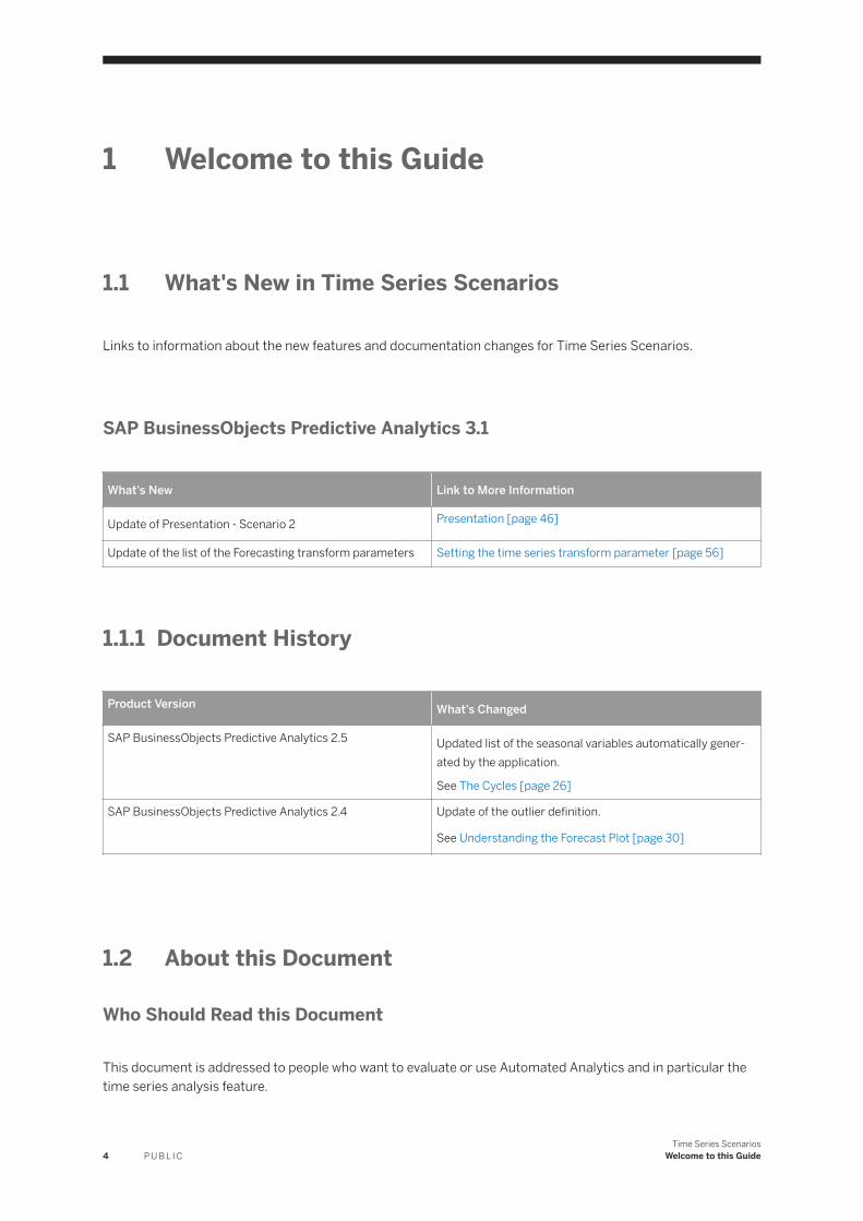
SAP BusinessObjects Predictive Analytics 3.1

What's New Link to More Information

Update of Presentation - Scenario 2 Presentation [page 46]

Update of the list of the Forecasting transform parameters Setting the time series transform parameter [page 56]

1.1.1 Document History

Product Version What's Changed

SAP BusinessObjects Predictive Analytics 2.5 Updated list of the seasonal variables automatically generated by the application.

See The Cycles [page 26]

SAP BusinessObjects Predictive Analytics 2.4 Update of the outlier definition.

See Understanding the Forecast Plot [page 30]

1.2 About this Document

Who Should Read this Document

This document is addressed to people who want to evaluate or use Automated Analytics and in particular the time series analysis feature.


Welcome to this Guide

Prerequisites for Use of this Document

Before reading this guide, you should read chapters 2 and 3 of the Classification, Regression, Segmentation and Clustering Scenarios - Automated Analytics User Guide that present respectively:

● An introduction to Automated Analytics● The essential concepts related to the use of Automated Analytics features

This guide is available on the SAP Help Portal at http://help.sap.com/pa.

What this Document Covers

This document introduces you to the main functionalities of the time series feature. Using the application scenario you can create your first models with confidence.

Modeler lets you build predictive models from data representing time series. With a time series analysis, you can:

● Identify and understand the phenomenon represented by your time series.● Forecast the evolution of time series in the short and medium term, that is, predict their future values.

1.3 Before Beginning

1.3.1 Files and Documentation Provided with this Guide

Sample Data Files

Automated Analytics is supplied with sample data files. These files allow you to take your first steps using various features of the application, and evaluate them.

During installation of SAP BusinessObjects Predictive Analytics, the following sample files for time series analysis are saved under the folder <installation directory>/Samples/KTS/:

● R_ozone-la.txt,● CashFlows.txt,● KxDesc_CashFlows.txt.

Documentation

Full Documentation Complete documentation can be found on the SAP Help Portal at http://help.sap.com/pa.

Time Series ScenariosWelcome to this Guide P U B L I C 5

http://help.sap.com/pa

http://help.sap.com/pa

Contextual HelpMost screens in the application are accompanied by contextual help that describes the options presented to you, and the concepts required for their application.

1.3.2 Displaying the Contextual Help

Each screen in Automated Analytics is accompanied by contextual help that describes the options presented to you, and the concepts required for their application.

1. To display the contextual help, press F1.2. To acces a searchable version of all the help for the application, select HelpOpen Full Searchable Help.


Welcome to this Guide

2 General Introduction to Scenarios

2.1 Scenario 1

This scenario demonstrates how to use a time series analysis for creating a standard model.

The data used in this scenario are monthly averages of hourly ozone (O3) readings in downtown Los Angeles from 1955 to 1972.

Ozone is a gas providing a protective shield against the ultraviolet radiation. When found in the lower atmosphere, it is a major component of smog. Thus ozone rate is a common measure for smog intensity.

Los Angeles municipality took three measures in order to reduce this level and so decrease the smog downtown:

● in 1960, the Golden State Freeway, which sails round downtown, opened,● in the same year, the rule 63 came into effect, lowering the amount of allowable reactive hydrocarbons in

gasoline,● in 1966, emission regulations for new car engines were introduced.

The purpose of this scenario is to confirm the decreasing trend of the ozone rate by predicting the next 18 months and describing the different signal elements based on the ozone rate.

2.2 Scenario 2

This scenario demonstrates how to use a time series analysis to create a model with extra predictable inputs.

In this scenario, you are an executive of a financial entity that manages cash-flows. Your role is to make sure that credits are available with the correct amount at the correct date to provide the best management possible of your financial flows.

Time series provides you with two methods for reaching your objective:

● creating a standard model,● creating a model with extra predictable variables.

2.3 Introduction to Sample Files

Automated Analytics provides sample data files allowing you to evaluate the time series analysis feature and take your first steps in using it.

Time Series ScenariosGeneral Introduction to Scenarios P U B L I C 7

The file R_ozone-la.txt is the sample data file that you will use to follow Scenario 1. It is an excerpt from the book Time Series Analysis: Forecasting and Control (G.E.P. Box and G.M. Jenkins), Third Edition, Prentice-Hall, 1994.

This file presents monthly averages of hourly ozone (O3) readings in downtown Los Angeles from 1955 to 1972. Each observation is characterized by 2 data items. These data, or variables, are described in the following table.

Variable Description Example of Values

Time Month and year of the readings

A date in the format yyyy-mm-dd, such as 1955-01-28

R_ozone-la Average of the hourly readings for the month

A numerical value with two decimals

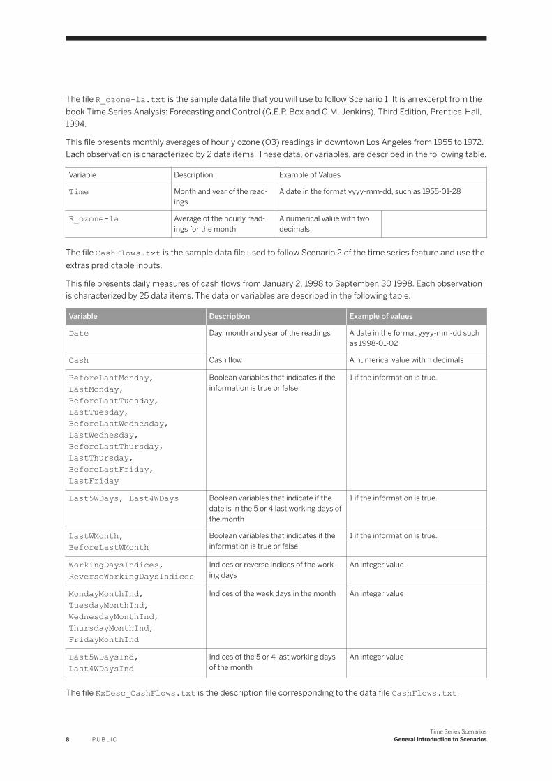
The file CashFlows.txt is the sample data file used to follow Scenario 2 of the time series feature and use the extras predictable inputs.

This file presents daily measures of cash flows from January 2, 1998 to September, 30 1998. Each observation is characterized by 25 data items. The data or variables are described in the following table.

Variable Description Example of values

Date Day, month and year of the readings A date in the format yyyy-mm-dd such as 1998-01-02

Cash Cash flow A numerical value with n decimals

BeforeLastMonday, LastMonday, BeforeLastTuesday, LastTuesday, BeforeLastWednesday, LastWednesday, BeforeLastThursday, LastThursday, BeforeLastFriday, LastFriday

Boolean variables that indicates if the information is true or false

1 if the information is true.

Last5WDays, Last4WDays Boolean variables that indicate if the date is in the 5 or 4 last working days of the month


LastWMonth, BeforeLastWMonth

Boolean variables that indicates if the information is true or false


WorkingDaysIndices, ReverseWorkingDaysIndices

Indices or reverse indices of the working days

An integer value

MondayMonthInd, TuesdayMonthInd, WednesdayMonthInd, ThursdayMonthInd, FridayMonthInd

Indices of the week days in the month An integer value

Last5WDaysInd, Last4WDaysInd

Indices of the 5 or 4 last working days of the month

An integer value

The file KxDesc_CashFlows.txt is the description file corresponding to the data file CashFlows.txt.


General Introduction to Scenarios

2.3.1 Additional Sample Files

Additional sample files are provided to further test time series:

● Lag1AndCycles.txt● Lag1AndCyclesAndWn.txt● TrendAndCyclic.txt● TrendAndCyclicAnd_4Wn.txt● TrendAndCyclicAndWn.txt

These files are located in the folder Samples\KTS.

2.4 File Format Specifications

A training data file for time series must contain at least two columns:

● The date column,● The signal column.

Three formats are supported for the Date column:

● datetime (ISO format: yyyy-mm-dd hh:mm), which has an hour-precision.● date (ISO format: yyyy-mm-dd), which has a day-precision.● number (number, for example "seconds").

The signal column (that is, the target variable) must be continuous

An optional weight column can be used to tweak the modeling procedure. Setting the weight of some rows to 0 allows ignoring these rows during the modeling process. By default, when a weight variable is not provided, all rows have a weight of 1.

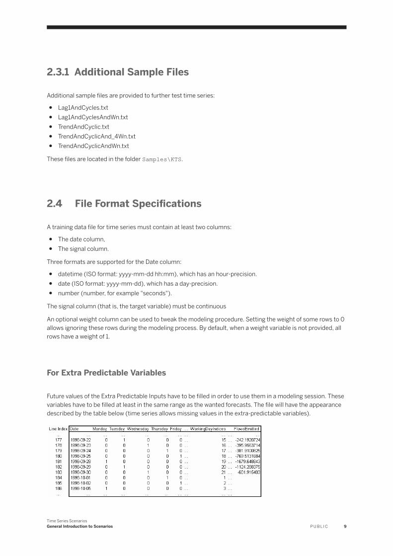
For Extra Predictable Variables

Future values of the Extra Predictable Inputs have to be filled in order to use them in a modeling session. These variables have to be filled at least in the same range as the wanted forecasts. The file will have the appearance described by the table below (time series allows missing values in the extra-predictable variables).

Time Series ScenariosGeneral Introduction to Scenarios P U B L I C 9

The last known signal value is at the line 183 with the corresponding date 1998-09-30. This line corresponds to the end of the training data set. The figures present after this line are the future values of the extras predictable variables: these figures are considered as predictive information.

Please note that the date variable has a special status. This variable is not considered as an extra predictable input; nevertheless it is possible to fill its future values. If you fill this variable in the predicted range, the application uses the values for forecasting. If you don’t, it generates the future dates. This is true whether extra predictable variables exist or not. This feature can be very useful if you are not satisfied by the dates automatically generated by the application.

The same file format has to be used for the training data set and the application data set.

NoteIf you want to use your own dates instead of the automatic date generation, please follow the same steps as the addition of extras predictable inputs.

2.5 Starting a Time Series Analysis

To accomplish the scenario, you will use the Java-based graphical interface of the application. SAP BusinessObjects Predictive Analytics allows you to select the features with which you will work, and help you at all stages of the modeling process

To Start SAP BusinessObjects Predictive Analytics

1. Select Start Programs SAP Business Intelligence SAP BusinessObjects Predictive Analytics Desktop SAP BusinessObjects Predictive Analytics

SAP BusinessObjects Predictive Analytics appears.2. Select Modeler, and thenCreate a Time Series Analysis.


General Introduction to Scenarios

3 Scenario 1: Standard Modeling with Time Series

Data modeling with time series is subdivided into four broadly defined stages:

1. Defining the Modeling Parameters2. Generating and Validating the Model3. Analyzing and Understanding the Analytical Results4. Using a Generated Model

3.1 Application Options

On every screen of the application, one or more of the following options may be available in a toolbar located under the screen title.

● Printing the screen,● Saving the screen content,● Copying the screen content,● Displaying the contextual Help.

3.1.1 Printing the Screen

To Print the Screen

1. Click the Print button.

A dialog box appears, asking you to select the printer to use.2. Select the printer to use and set other print properties if need be.3. Click OK.

The screen content is printed.

3.1.2 Saving the Screen Content

1. Click the Save button.

A dialog box appears, asking you to select the file properties2. Type a name for your file.

Time Series ScenariosScenario 1: Standard Modeling with Time Series P U B L I C 11

3. Select the destination folder.4. Click OK.

If the screen displays:

○ A graph, it is saved as a PNG image○ A report, it is saved as an HTML file

3.1.3 Copying the Screen Content

Click the Copy button.

If the screen displays:

○ A report, the application copies its HTML code. You can paste it into a word processing program or into a spreadsheet program (such as Excel) and use it to generate your own graph.

○ A graph, the application copies its parameters. You can paste it into a spreadsheet program (such as Excel) and use it to generate your own graph.

3.2 Step 1 - Defining the Modeling Parameters

3.2.1 Selecting a Data Source

For this scenario, use the file R_ozone-la.txt as a training data set.

To Select a Data Source:

1. On the screen Select a Data Source, select the option Data Type to select the data source format to be used.

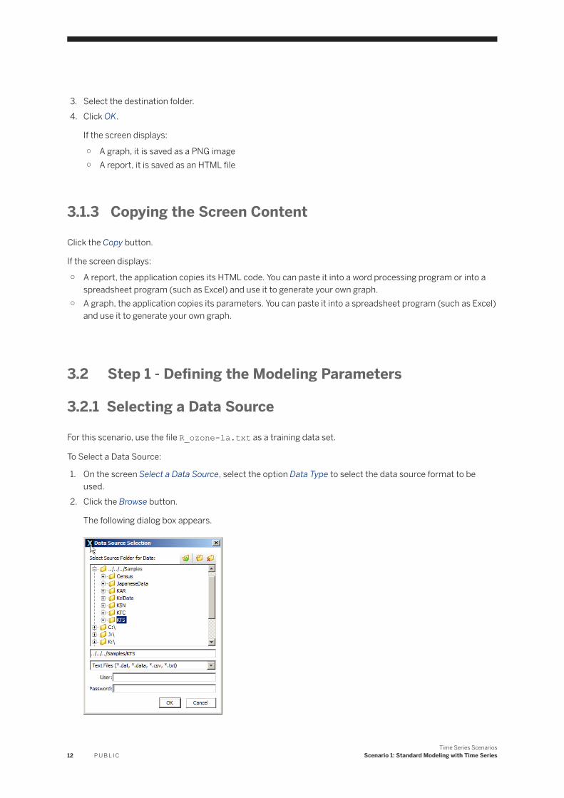
2. Click the Browse button.

The following dialog box appears.


Scenario 1: Standard Modeling with Time Series

3. Double-click the Samples folder, then the KTS folder.

NoteDepending on your environment, the Samples folder may or may not appear directly at the root of the list of folders. If you selected the default settings during the installation process, you will find the Samples folder located in C:\Program Files\SAP BusinessObjects Predictive Analytics.

4. Select the file R_ozone-la.txt, then click OK.

The name of the file appears in the Data Set field.

3.2.2 Selecting a Cutting Strategy

To generate a time series model, you must select a cutting strategy to cut your training data set into the three sub-sets: estimation, validation and test. Since the order of the observations in the data set is important for the modeling, only two types of cutting strategies are available in time series:

● Sequential with Test● Sequential without Test

For more information on Cutting Strategies, see the Classification, Regression, Segmentation and Clustering Scenarios - Automated Analytics User Guide.

3.2.2.1 Selecting a Cutting Strategy

For this Scenario, do not change the cutting strategy by default.

1. On the screen Select a Data Source, click the button Cutting Strategy.

The panel Cutting Strategy is displayed.2. In the Predefined list, select the cutting strategy you want to use.3. Click the OK button.4. Back to the panel Select a Data Source, click the Next button.5. The screen Data Description appears.6. Go to the section Describing the Data Selected.

3.2.3 Describing the Data Selected

To describe your data, you can:

● Use an existing description file, that is, taken from your information system or saved from a previous use of Automated Analytics.

● Or create a description file using the Analyze option. In this case, it is important that you validate the description file obtained. You can save this file for later re-use.


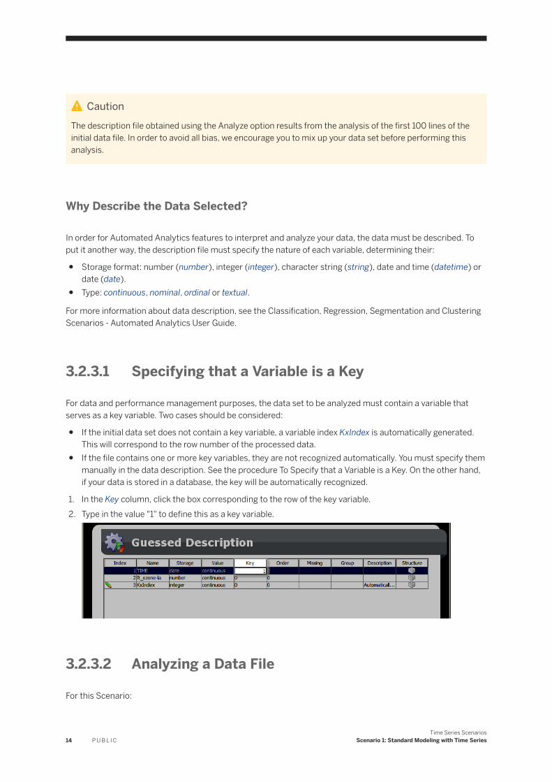
CautionThe description file obtained using the Analyze option results from the analysis of the first 100 lines of the initial data file. In order to avoid all bias, we encourage you to mix up your data set before performing this analysis.

Why Describe the Data Selected?

In order for Automated Analytics features to interpret and analyze your data, the data must be described. To put it another way, the description file must specify the nature of each variable, determining their:

● Storage format: number (number), integer (integer), character string (string), date and time (datetime) or date (date).

● Type: continuous, nominal, ordinal or textual.

For more information about data description, see the Classification, Regression, Segmentation and Clustering Scenarios - Automated Analytics User Guide.

3.2.3.1 Specifying that a Variable is a Key

For data and performance management purposes, the data set to be analyzed must contain a variable that serves as a key variable. Two cases should be considered:

● If the initial data set does not contain a key variable, a variable index KxIndex is automatically generated. This will correspond to the row number of the processed data.

● If the file contains one or more key variables, they are not recognized automatically. You must specify them manually in the data description. See the procedure To Specify that a Variable is a Key. On the other hand, if your data is stored in a database, the key will be automatically recognized.

1. In the Key column, click the box corresponding to the row of the key variable.2. Type in the value "1" to define this as a key variable.

3.2.3.2 Analyzing a Data File

For this Scenario:



● Select Text Files as the file type.● Use the Analyze function to describe the R_ozone-la.txt data file.● Set the TIME variable as the key.● Set the KxIndex variable Key to 0.● Set the TIME variable Order to 1.

1. On the screen Data Description, click the Analyze button.

The file description is displayed.2. Validate the description (storage type and value).3. Click the Next button.

3.2.4 Selecting Variables

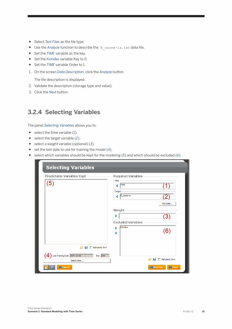
The panel Selecting Variables allows you to:

● select the time variable (1),● select the target variable (2),● select a weight variable (optional) (3),● set the last date to use for training the model (4),● select which variables should be kept for the modeling (5) and which should be excluded (6).


3.2.4.1 Selecting a Time Variable

For this Scenario:

● Keep TIME as the time variable.● Keep R_ozone-la as the target variable.● Do not select a weight variable.● Keep the last training date selected by default.

1. On the screen Selecting Variables, in the section Predictable Variables Kept (left hand side), select the variable you want to use as the time variable.

2. Click the button > located on the left of the Time field in section Required Variable (upper right hand side). The variable moves to the Time field.

NoteTo remove the time variable, select the variable in the Time field and click the button < to move the variables back to the screen section Predictable Variables Kept.

3.2.4.2 Selecting a Target Variable

1. On the screen Selecting Variables, in the section Predictable Variables Kept (left hand side), select the variable you want to use as the Target Variable.

2. Click the button > located on the left of the Target field in section Required Variable (upper right hand side).

The variable moves to the Target field.

NoteTo remove the target variable, select the variable in the Target field and click the button < to move the variables back to the screen section Predictable Variables Kept.

3.2.4.3 Selecting a Weight Variable

1. In the field Predictable Variables Kept, select the weight variable.2. Click the > button located on the right of the Weight field.

NoteTo remove the weight variable, select the Weight field and click the < button.



3.2.4.4 Excluding Variables

1. In the field Predictable Variables Kept (left hand side), select the variables you want to exclude.

NoteTo select all the variables of a field, click inside the field and push the keys Ctrl and A at the same time.

2. Click the > button located near the top right corner of the field Excluded Variable.

3.2.4.5 Displaying the Signal

1. On the screen Selecting Variables, click the button Plot Data..., located in the section Required Variables. The screen Display Signal is displayed.

2. Click the Time list and select the variable containing the time information.

NoteBy default, time series uses the first column of the data set as time variable.

3. Click the Signal list and select the variable containing the signal information.4. Click the Previous button to go back to the screen Selecting Variables.

3.2.4.6 Reducing the Training Data Set

The last date found in the data set is automatically selected as the last training date. The second field, which indicates the number of the line in the data set, is automatically updated depending on the date you have selected.

1. On the screen Selecting Variables, click the button Select Date.... The panel Sample Data View is displayed.2. Uses the First Row Index and Last Row Index to display the line containing the date you want to select as

the last training date.3. Click the Refresh button to update the list of rows displayed.4. Click the row corresponding to the date you want to select. The selected row is displayed in the section

Current Selection at the bottom of the panel.5. Click the OK button to validate your selection. The window closes and the Last Training Date information

are updated in the main panel.

3.2.5 Checking Modeling Parameters

The screen Summary of Modeling Parameters allows you to check the modeling parameters just before generating the model.


● The name of the model is filled automatically. It corresponds to the name of the target variable (R_ozone-la for this scenario), followed by the underscore sign ("_") and the name of the data source, without its file extension (R_ozone-la in this case).

● The field Number of Forecast(s) allows you to select the number of forecasts to generate. The time unit used is determined by the data analyzed. For example, if the data set observations are recorded monthly, the time unit will be one month. See section Defining the Number of Forecasts.The maximum number of forecasts allowed is indicated in the field Maximum Forecast. This number depends on the number of extra predictable variables available. If there is no extra predictable variables, the number of forecasts is unlimited.

● The Autosave button allows you to activate the feature that will automatically save the model once it has been generated. When the autosave option is activated, a green check mark is displayed on the Autosave button.

Defining the Number of Forecasts

For this Scenario, define the number of forecasts to 24, that is, two years.

To Define the Forecasts Number, on the screen Summary of Modeling Parameters, in the field Number of Forecast(s), enter the number of forecasts you want to obtain.

3.2.5.1 Defining the Advanced Parameters

The advanced parameters allow you to:

● limit the number of analyzed variables,● define the modeling procedure.

1. Click the Advanced button. The panel Specific Parameters of the Model is displayed.2. Set the parameters as explained in the following sections.3. Click the OK button to save the new parameters. The panel Summary of Modeling Parameters is displayed.

3.2.5.2 Defining the Number of Analyzed Variables (optional)

Time series automatically generates the variables that are necessary to the modeling. Among these, it is possible to reduce the number of the cyclic variables by changing the parameter Maximum Length of Analyzed Cycles and the lagged variables created by changing the parameter Maximum Order of the Autoregressive Model.

● The Maximum Length of Analyzed Cycles controls the way that time series analyzes the periodicities in the signal. This is the length of the longest cycle time series will try to detect. The default value is 450. It is also limited by the size of the estimation data set. You can disable the cyclic analysis by setting this parameter to zero.



NoteBy reducing the default number of variables generated by time series, you are able to reduce the computation time. However it is strongly recommended to use the default settings otherwise the quality of modeling could be compromised.

● The Maximum Order of the Autoregressive Model controls the way that time series analyzes the random fluctuations in the signal. This parameter defines the maximum dependency of the signal on its own past values. You can set this parameter to zero to disable the fluctuations analysis.

3.2.5.3 Defining the Other Modeling Options

The Ignore Outliers when Estimating the Trend checkbox uses a strategy for reducing the effect of outliers when estimating the regressions in deterministic trends. This leads to an improvement in trend estimation.

The Force Positive Forecasts checkbox allows users to force time series to generate a positive model (with positive forecasts only).

3.2.5.4 Defining the Variables

This parameter groups some controls for the variable selection feature. When a variable selection is used, an automatic selection process is performed on trends or AR models during the competition and the result is kept only if it improves the final model.

● The Percentage of Variable Contributions to Keep is the percentage of contributions that are kept in the automatic selection process. The default value is 95%.

● The Activate for All Extra-predictable Based Trends option performs a variable selection on all extrapredictable-based trends. User variables are kept only if they have sufficient contributions in the trend regression. The checkbox is enabled by default.

● The Activate for All Autoregressive Models option performs an automatic variable selection on the past values of the signal for all autoregressive models. This leads to a more parsimonious AR model, that is a simpler model and a lower order. The box is not checked by default.

3.2.5.5 Modify the Modeling Procedure

You can select one of the following types of modeling procedure:

Default corresponds to the standard Time Series modeling

Only Based on Extra-Predictable Variables works as a Classification/Regression model build on the extra-predictable variables with the signal as the target. This mode can be used to refine and validate the extra-predictable variables or to identify useless ones.


Disable the Polynomial Trends generates all the models but those containing a polynomial trend.

Customized allows you to enable/disable the types of models that will be generated by Time Series when analyzing the signal. The following table lists the types of models that can be disabled.

Types of models that can be disabled when using the Customized modeling procedure.

Component Model Type Description

Trends Lag1 Previous value of the signal

Lag2 Value before previous

Second Order Differencing Trend using double-differencing to propagate the slope of the signal

Linear in Time Linear regression on the time

Polynomial in Time Polynomial regression on the time

Linear in ExtraPredictables Linear regression on the extra-predictable variables

Linear in Time and Linear in ExtraPredictables

Linear regression on the time and extra-predictable variables

Polynomial in Time and Linear in ExtraPredictables

Polynomial regression on the time and linear regression on the extra-predictable variables

Periodicities Cyclics Detection of cyclic variables

Seasonalities Detection of seasonal variables

Periodic Extrapredictables Extra-predictable usage as Periodics

Fluctuations Autoregressive Autoregressive modeling

3.2.5.6 Modifying the Modeling Procedure

1. In the section Modify the Modeling Procedure, check the desired option.2. If you have selected the Customized option, uncheck the types of models you want to disable.3. Click the OK button. The panel Summary of Modeling Parameters is displayed.

3.2.5.7 Activating the Autosave Option

The Model Autosave panel allows you to activate the option that will automatically save the model at the end of the generation process and to set the parameters needed when saving the model.

To activate the option, proceed as follows:

1. In the Summary of Modeling Parameters panel, click the Autosave button.The Model Autosave panel is displayed.



2. Check Enable Model Autosave.3. Set the parameters listed in the following table.

Parameter Description

Model Name This field allows you to associate a name with the model. This name will then appear in the list of models to be offered when you open an existing model.

Description This field allows you to enter the information you want, such as the name of the training data set used, the polynomial degree or the performance indicators obtained. This information could be useful to you later for identifying your model.

Note that this description will be used instead of the one entered in the Summary of Modeling Parameters panel.

Data Type This list allows you to select the type of storage in which you want to save your model. The following options are available:○ Text Files, to save the model in a text file.○ Data Base, to save the model in a database.○ Flat Memory, to save the model in the active memory.

Folder Depending upon which option you selected, this field allows you to specify the ODBC source, the memory store or the folder in which you want to save the model.

File/Table This field allows you to enter the name of the file or table that is to contain the model. When saving the model as a text file, you must enter one of the following format extensions .txt (text file in which the data is separated by tabs) or .csv (text file in which the data is separated by commas).

4. Click OK.

3.3 Step 2 - Generating the Model

3.3.1 Generating the Model

Once the modeling parameters are defined, you can generate the model.

1. On the screen Summary of Modeling Parameters, click the Generate button. The screen Training the Model appears. The model is being generated. A progress bar allows you to follow the process.

2. If the Autosave option has been activated in the panel Summary of Modeling Parameters, a warning message is displayed at the end of the learning process confirming that the model has been saved.

3. Click Close.

3.3.2 Following the Progress of the Generation Process

There are two ways for you to follow the progress of the generation process:

● The Progress Bar displays the progression for each step of the process. It is the screen displayed by default.


● The Detailed Log displays the details of each step of the process.

To display the Progression Bar

Click View Type and select ( Progress).

The progression bar screen appears.

To Display the Detailed Log

Click View Type and select the ( Log) button.

The detailed log displays the details of each step of the process.

To Stop the Learning Process

1. Click the ( Stop Current Task) button.2. Click the Previous button.

The screen Summary of Modeling Parameters appears.3. Go back to the section on checking modeling parameters.

3.3.3 Visualizing the Model Results

At the end of the generation process, a summary of the model results appears.

If you have built more than one model in the same session, all model debriefing will be displayed on this screen sorted by Date of Build.

For more information on the model summary, go to section Understanding the Model Debriefing.

CautionIn some cases, the message No Model Found is displayed instead of the signal information. It means that none of the models found can predict accurately the signal evolution.



3.4 Step 3 - Analyzing and Understanding the Generated Model

The suite of plotting tools within the application allows you to analyze and understand the model generated:

● The performance of the model,● The forecasts generated by the model.

3.4.1 Model Debriefing

3.4.1.1 To Display the Model Debriefing

On the Using the Model menu, select the Model Overview option.

The screen Model Overview appears.

NoteIf you have built more than one model in the same session, all model debriefing will be displayed on this screen sorted by Date of Build.

3.4.1.2 Understanding the Model Debriefing

The Model Debriefing screen is composed of four sections detailing information on:

● The overview of the model● The targets statistics● The model components● The model performance

3.4.1.3 The Model Overview

This section details the following information:

Name Significance For this scenario...

Model Name Name of the model.

It is generated by using the target variable name and the data set name

R_ozone-la_R_ozone-la


Data Set Name of the data source used for the model

R_ozone-la.txt

Initial Number of Input Variables

Total number of variables in the data set

3

Number of Selected Variables

Number of variables used to generate the model

1

Number of Records Number of observation in the data source file

204

Building Date Date and time when the model was build

2015-03-10 10:51:26

Learning Time Duration of the learning process 3s

Engine Name Name of the component used to build the model

Kxen.TimeSeries

3.4.1.4 The Targets Statistics

For continuous targets:

Name Significance For this scenario...

<target name> name of the target variable for which the statistics are stated

R_ozone-la

Min Minimum value found in the data set for the target variable

1.33

Max Maximum value found in the data set for the target variable

7.54

Mean Mean of the target variable 3.662

Standard Deviation Measure of the extent to which the target values are spread around their average

1.29

3.4.1.5 The Signal Components

This section details the model components, that is the components of the polynomial used to generated the forecasts.

A model is a combination of at least one of the three following types of elements:

● one trend,● one or more cycles,● one fluctuation.



3.4.1.6 The Trend

The trend is the general orientation of the signal. The four types of trends are detailed in the following table:

Type of trend Can be displayed as...

Polynom(Time) a curve corresponding to the detected polynomial. A polynomial is modeled using Classification/Regression.

The available functions for the polynomial are Time, square(Time), sqrt(Time), where Time equals the value of the DateColumnName parameter.

Polynom(Time, ExtraPredictable) a curve corresponding to the detected polynomial.

This is the same function using in addition the extra predictable variables as inputs.

Linear(Time) a straight line.

It is a special case of Polynom(Time) .

Linear(Time, ExtraPredictables) a straight line.

This is the same function using in addition the extra predictable variables as inputs.

Polynom (ExtraPredictables) a curve corresponding to the detected polynomial.

This function could be very next to a cyclic representation because Classification/Regression is only using the extra-predictable variables as inputs.

L1 the signal moved one step forward.

This is the basic forecast where the predicted observation equals the latest signal observation.

L2 the signal moved two step forward.

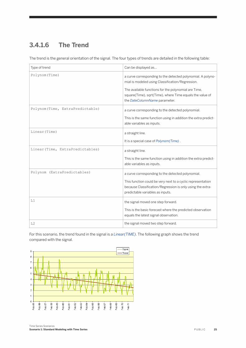
For this scenario, the trend found in the signal is a Linear(TIME). The following graph shows the trend compared with the signal.


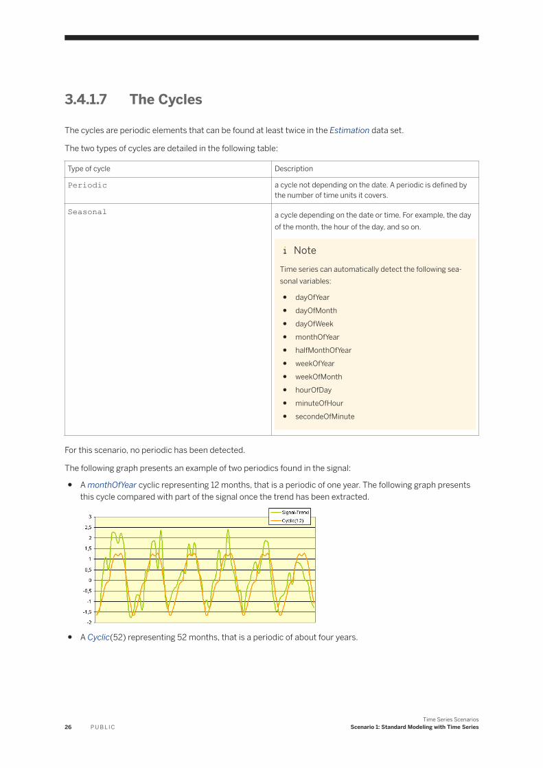
3.4.1.7 The Cycles

The cycles are periodic elements that can be found at least twice in the Estimation data set.

The two types of cycles are detailed in the following table:

Type of cycle Description

Periodic a cycle not depending on the date. A periodic is defined by the number of time units it covers.

Seasonal a cycle depending on the date or time. For example, the day of the month, the hour of the day, and so on.

NoteTime series can automatically detect the following seasonal variables:

● dayOfYear● dayOfMonth● dayOfWeek● monthOfYear● halfMonthOfYear● weekOfYear● weekOfMonth● hourOfDay● minuteOfHour● secondeOfMinute

For this scenario, no periodic has been detected.

The following graph presents an example of two periodics found in the signal:

● A monthOfYear cyclic representing 12 months, that is a periodic of one year. The following graph presents this cycle compared with part of the signal once the trend has been extracted.

● A Cyclic(52) representing 52 months, that is a periodic of about four years.



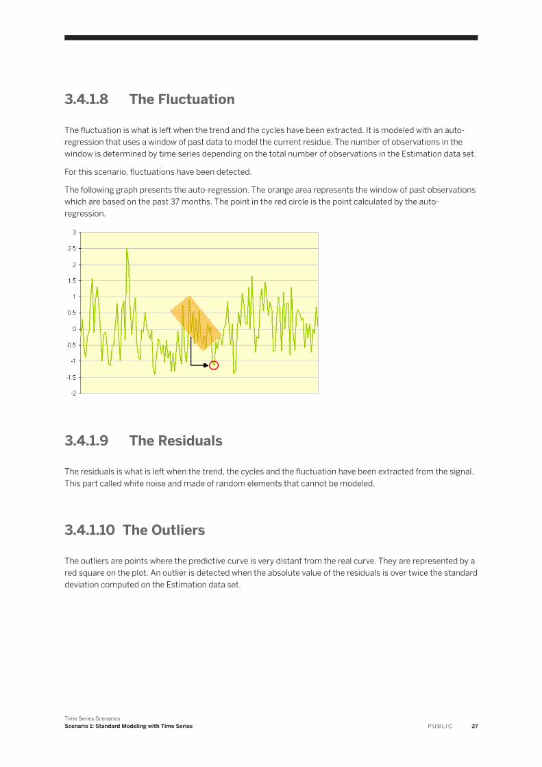
3.4.1.8 The Fluctuation

The fluctuation is what is left when the trend and the cycles have been extracted. It is modeled with an auto-regression that uses a window of past data to model the current residue. The number of observations in the window is determined by time series depending on the total number of observations in the Estimation data set.

For this scenario, fluctuations have been detected.

The following graph presents the auto-regression. The orange area represents the window of past observations which are based on the past 37 months. The point in the red circle is the point calculated by the auto-regression.

3.4.1.9 The Residuals

The residuals is what is left when the trend, the cycles and the fluctuation have been extracted from the signal. This part called white noise and made of random elements that cannot be modeled.

3.4.1.10 The Outliers

The outliers are points where the predictive curve is very distant from the real curve. They are represented by a red square on the plot. An outlier is detected when the absolute value of the residuals is over twice the standard deviation computed on the Estimation data set.


3.4.1.11 The Model Performance

This section gives the model performance.

Name Significance For this Scenario

Horizon-Wide MAPE This quality indicator for the forecasting model is the mean of MAPE values observed over all the training horizon. A value of zero indicates a perfect model while values above 1 indicate bad quality models. A value of 0.09 means that the model takes into account 91% of the signal or , in other words, the forecasting error (model residues) is relatively of 9%.

MAPE - Mean Absolute Percentage Error : The MAPE value is the average of the sum of the absolute values of the percentage errors. It measures the accuracy of the model's forecasts and indicates how much the forecasts differ from the real signal value.

0.178

3.4.2 Forecasts

3.4.2.1 Displaying the Forecast Plot

1. On the Using the Model menu, click the View Forecasts option.2. A pop-up is displayed asking you to confirm or update the name and location of the training data set file.3. Update the information if you have renamed or moved the training data set file, or if its type has been

changed.

NoteSteps 2 and 3 are required in case you open a saved model and the data set used to train it has been moved, for example.

4. Click OK.

The screen View Forecasts appears.

NoteWhen you copy and paste the graph, the confidence interval information are not made available. To get this information, you can go to Tables Debriefing Error Bars . The interval lower bound equals the



signal value minus two times the value of the error bar and the upper bound equals the signal value plus two times the value of the error bar.

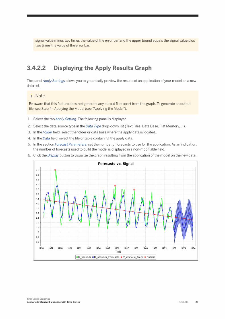
3.4.2.2 Displaying the Apply Results Graph

The panel Apply Settings allows you to graphically preview the results of an application of your model on a new data set.

NoteBe aware that this feature does not generate any output files apart from the graph. To generate an output file, see Step 4 - Applying the Model (see "Applying the Model").

1. Select the tab Apply Setting. The following panel is displayed.

2. Select the data source type in the Data Type drop-down list (Text Files, Data Base, Flat Memory, ...).3. In the Folder field, select the folder or data base where the apply data is located.4. In the Data field, select the file or table containing the apply data.5. In the section Forecast Parameters, set the number of forecasts to use for the application. As an indication,

the number of forecasts used to build the model is displayed in a non-modifiable field.6. Click the Display button to visualize the graph resulting from the application of the model on the new data.


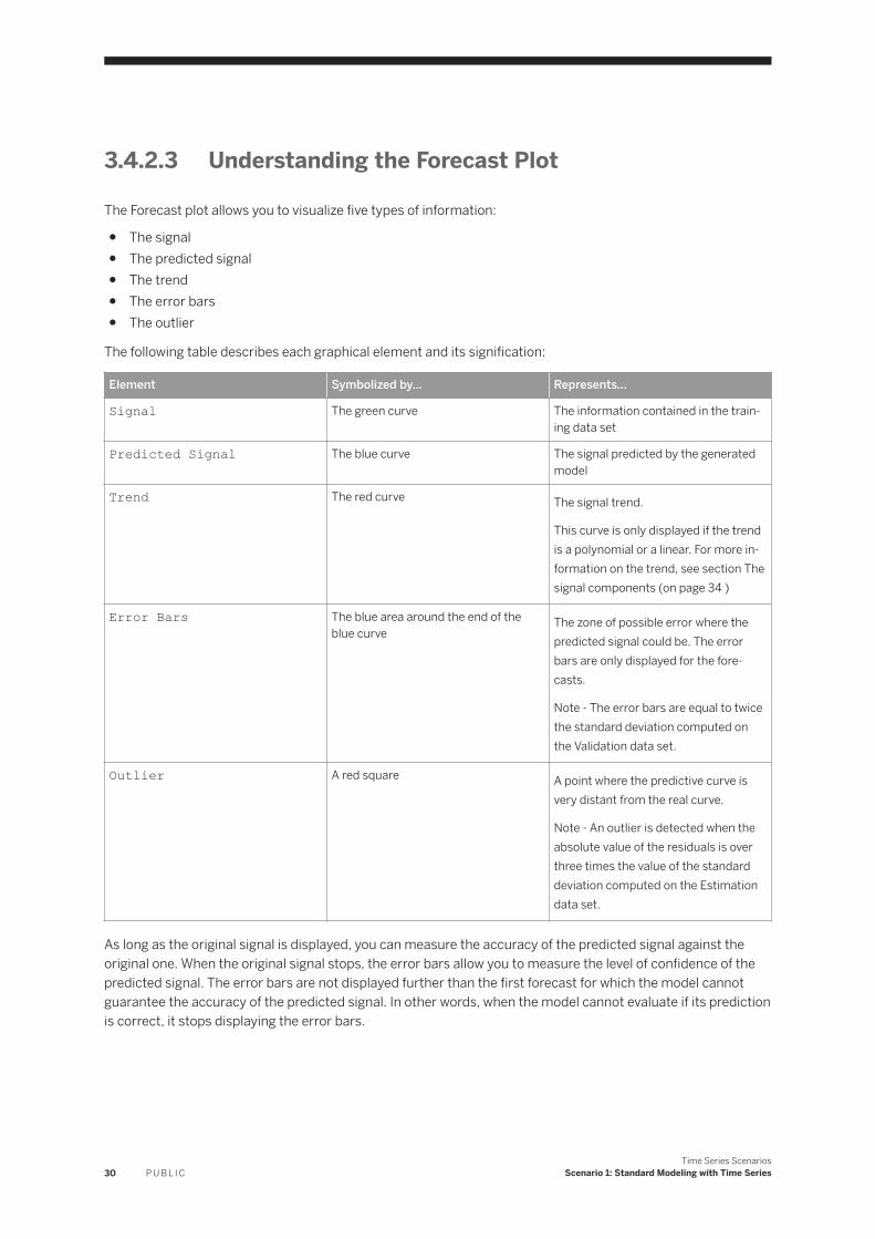
3.4.2.3 Understanding the Forecast Plot

The Forecast plot allows you to visualize five types of information:

● The signal● The predicted signal● The trend● The error bars● The outlier

The following table describes each graphical element and its signification:

Element Symbolized by... Represents...

Signal The green curve The information contained in the training data set

Predicted Signal The blue curve The signal predicted by the generated model

Trend The red curve The signal trend.

This curve is only displayed if the trend is a polynomial or a linear. For more information on the trend, see section The signal components (on page 34 )

Error Bars The blue area around the end of the blue curve

The zone of possible error where the predicted signal could be. The error bars are only displayed for the forecasts.

Note - The error bars are equal to twice the standard deviation computed on the Validation data set.

Outlier A red square A point where the predictive curve is very distant from the real curve.

Note - An outlier is detected when the absolute value of the residuals is over three times the value of the standard deviation computed on the Estimation data set.

As long as the original signal is displayed, you can measure the accuracy of the predicted signal against the original one. When the original signal stops, the error bars allow you to measure the level of confidence of the predicted signal. The error bars are not displayed further than the first forecast for which the model cannot guarantee the accuracy of the predicted signal. In other words, when the model cannot evaluate if its prediction is correct, it stops displaying the error bars.



NoteIf you have selected the Sequential cutting strategy, the error bars are also displayed on the test part of the signal.

3.4.2.4 Zooming the Plot In/Out

1. Right-click the plot area you want to zoom in or out.

A contextual menu appears.2. Select the type of zoom you want to apply.3. Select on which axes you want to zoom. Note that the point where you click is the central point of the

zoom.

3.4.2.5 Displaying the Value of a Specific Element of a Signal

Place your cursor on a selected point of a signal curve.

A pop-up displays the information for this point of the signal.

3.4.3 Signal Components

3.4.3.1 Displaying the Signal Components

1. On the Using the Model menu, click the option View Signal Components.2. A pop-up is displayed asking you to confirm or update the name and location of the training data set file.3. Update the information if you have renamed or moved the training data set file, or if its type has been

changed.

NoteSteps 2 and 3 are required in case you open a saved model and the data set used to train it has been moved, for example.

4. Click OK.

The screen View Signal Components appears.5. In the list Display Options, select the component you want to display.


3.4.3.2 Understanding the Signal Components

The signal components are ordered as listed below:

1. the trend,2. the periodics,3. the fluctuation4. the residuals,5. the outliers.

To display a component, time series removes the previous existing components from the signal. For example, to display the fluctuation, time series removes the trend and the periodics from the signal.

More information on the signal components available in Understanding the Model Debriefing: Signal Components.

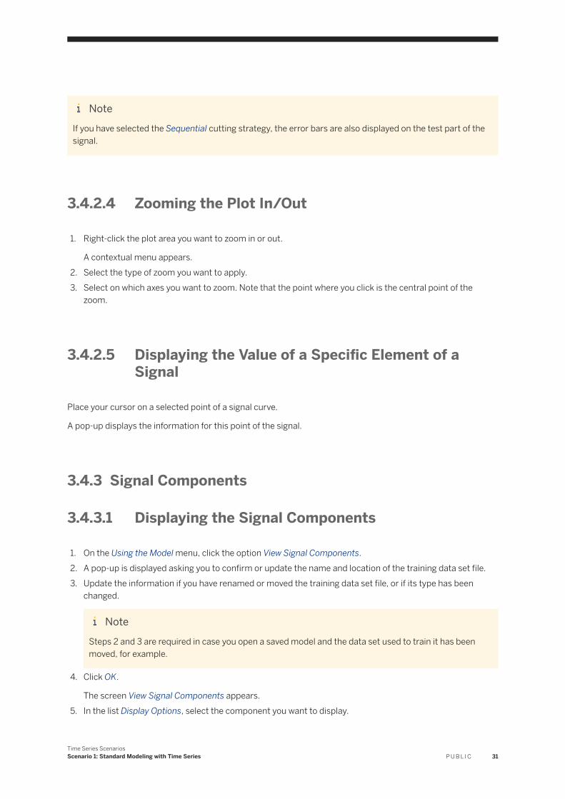
Signal vs. Trend

For this Scenario, Time series has recognized a descending linear trend, it appears in blue on the plot Signal vs. Trend.

The detailed explanation of the trend can be found in Understanding the Model Debriefing Signal Components The Trend (see "The Trend").

Signal vs. Periodics

For this scenario, the model has not found any periodic. A detailed explanation of the periodics can be found in section Understanding the Model Debriefing Signal Components The Cycles



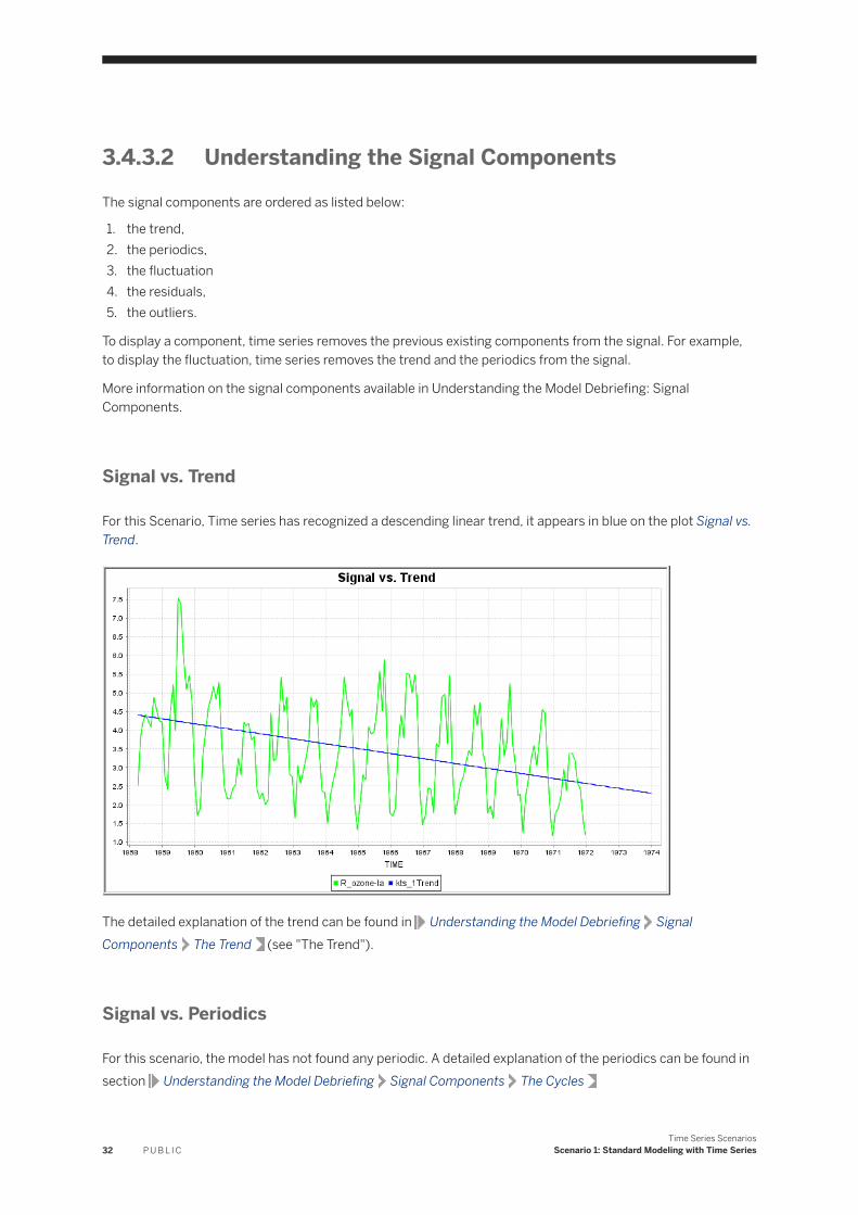
Signal vs. Fluctuation

For this scenario, time series has detected fluctuations that are represented in blue in the plot (Signal-Trend) vs. Fluctuation.

NoteYou can see that the trend has been removed from the signal to allow better visualization of the fluctuations.

A detailed explanation of the fluctuation can be found in section Understanding the Model Debriefing Signal Components The Fluctuation (see "The Fluctuation").

Signal vs. Residuals

For this scenario, the residuals found by the model appear in blue on the plot Signal vs. Final Residuals.


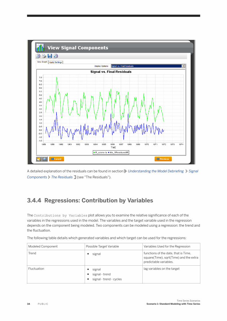
A detailed explanation of the residuals can be found in section Understanding the Model Debriefing Signal Components The Residuals (see "The Residuals").

3.4.4 Regressions: Contribution by Variables

The Contributions by Variables plot allows you to examine the relative significance of each of the variables in the regressions used in the model. The variables and the target variable used in the regression depends on the component being modeled. Two components can be modeled using a regression: the trend and the fluctuation.

The following table details which generated variables and which target can be used for the regressions:

Modeled Component Possible Target Variable Variables Used for the Regression

Trend ● signal functions of the date, that is Time, square(Time), sqrt(Time) and the extra predictable variables.

Fluctuation ● signal● signal - trend● signal - trend - cycles

lag variables on the target



The following four types of plots allow you to visualize contributions by variables :

● Variable Contributions● Variable Weights● Smart Variable Contributions● Maximum Smart Variable Contributions

The plot... Presents...

Variable Contributions The relative importance of each variable in the built model

Variable Weights The weights (in the final polynomial) of the normalized variables

Smart Variable Contributions The variables internal contributions

Maximum Smart Variable Contributions The variables internal contributions including only the maximum of similar variables. For example, only binned encoding of the continuous variable age will be displayed

3.4.4.1 Displaying the Variable Contributions

In this scenario, the model contains only the regression linear(TIME) which defines the trend.

1. On the screen Using the Model, click the option Regressions: Contributions by Variables.

The screen Contributions by Variable is displayed.2. Select the type of plot you want to display in the drop-down list Chart Type. The plot Maximum Smart

Variables is displayed by default.

NoteIn case of a regression on one variable only, the plot Maximum Smart Variables is not available. Use the drop-down list Chart Type to select another plot.

3. Select the regression you want to analyze in the Models drop-down list. Note that if there is only one regression in the model, the Models drop-down list is not displayed.

3.4.5 Statistical Reports

To help you analyze your modeling results and to enable you to possibly share these results with your colleagues, managers, partners or PUBLICs, time series provides you with a set of statistical reports in various formats.

There are three categories of reports:

● the Descriptive Statistics, which provide information on the variables used to generate the model, such as the variables types and categories, the data set size, the cross-statistics...

● the Performance Indicators, which provide information on the performance of the model thanks to various indicators such as the forecasts error bars and efficiency, the U2, the standard deviation, ...


● the Cyclic Variables, which provide you with an analysis of the seasonal and cyclic variables displayed as graphs.

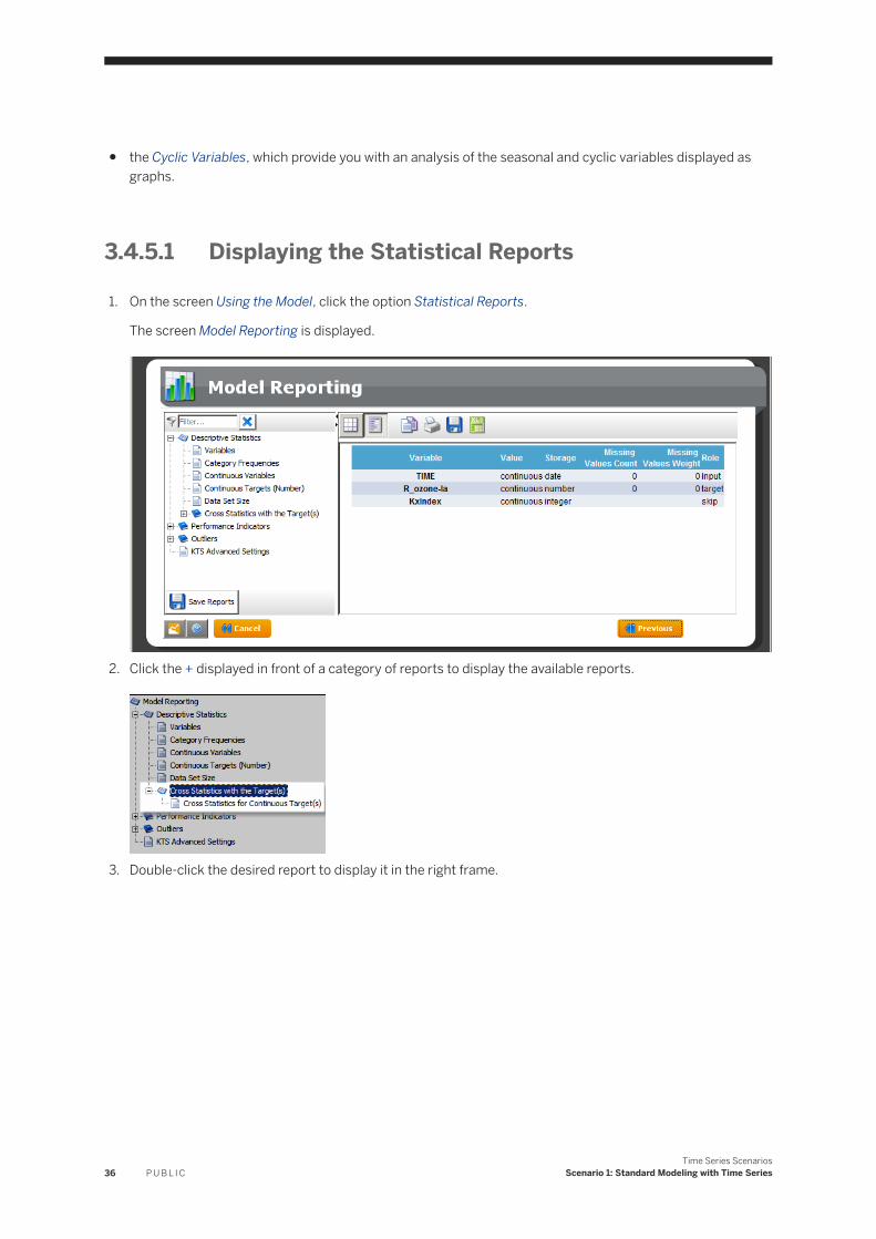
3.4.5.1 Displaying the Statistical Reports

1. On the screen Using the Model, click the option Statistical Reports.

The screen Model Reporting is displayed.

2. Click the + displayed in front of a category of reports to display the available reports.

3. Double-click the desired report to display it in the right frame.



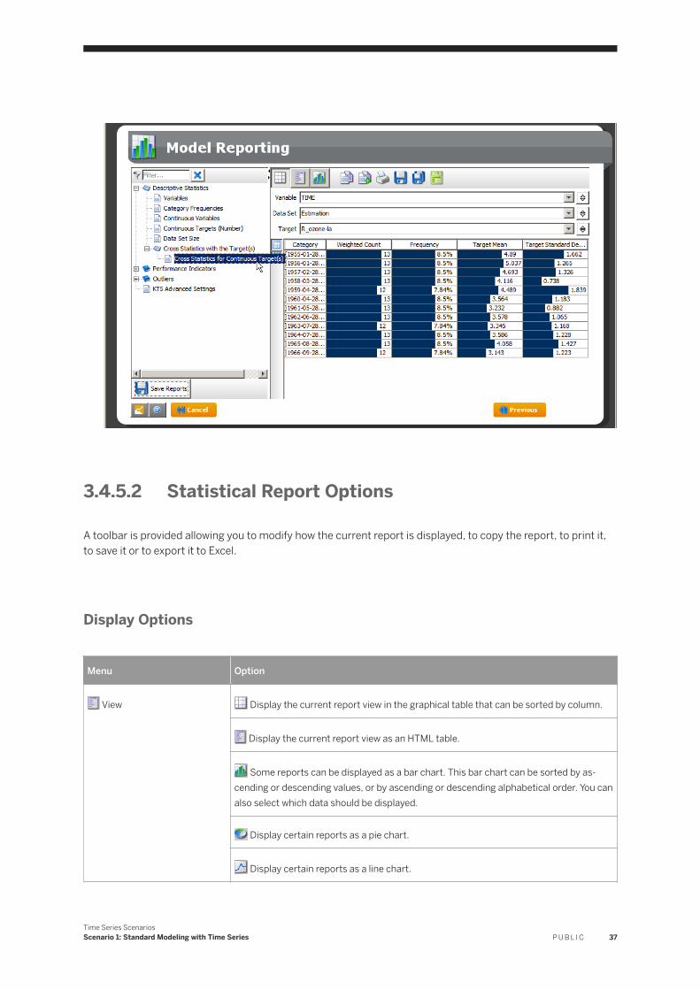
3.4.5.2 Statistical Report Options

A toolbar is provided allowing you to modify how the current report is displayed, to copy the report, to print it, to save it or to export it to Excel.

Display Options

Menu Option

View Display the current report view in the graphical table that can be sorted by column.

Display the current report view as an HTML table.

Some reports can be displayed as a bar chart. This bar chart can be sorted by ascending or descending values, or by ascending or descending alphabetical order. You can also select which data should be displayed.

Display certain reports as a pie chart.

Display certain reports as a line chart.


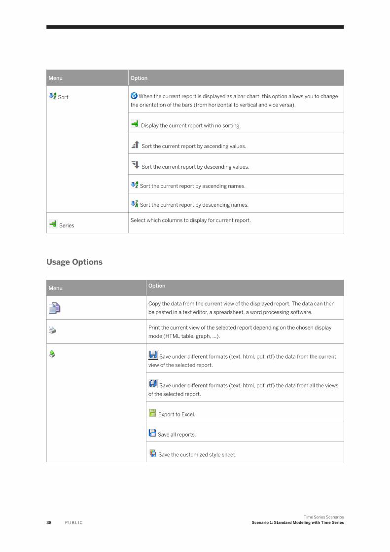
Menu Option

Sort When the current report is displayed as a bar chart, this option allows you to change the orientation of the bars (from horizontal to vertical and vice versa).

Display the current report with no sorting.

Sort the current report by ascending values.

Sort the current report by descending values.

Sort the current report by ascending names.

Sort the current report by descending names.

SeriesSelect which columns to display for current report.

Usage Options

Menu Option

Copy the data from the current view of the displayed report. The data can then be pasted in a text editor, a spreadsheet, a word processing software.

Print the current view of the selected report depending on the chosen display mode (HTML table, graph, ...).

Save under different formats (text, html, pdf, rtf) the data from the current view of the selected report.

Save under different formats (text, html, pdf, rtf) the data from all the views of the selected report.

Export to Excel.

Save all reports.

Save the customized style sheet.



3.5 Step 4 - Using the Model

Once generated, the model may be:

● applied to additional data sets. The model thus allows you to perform predictions on these application data sets, by predicting the values of a target variable.

● saved for later use.

3.5.1 Applying the Model

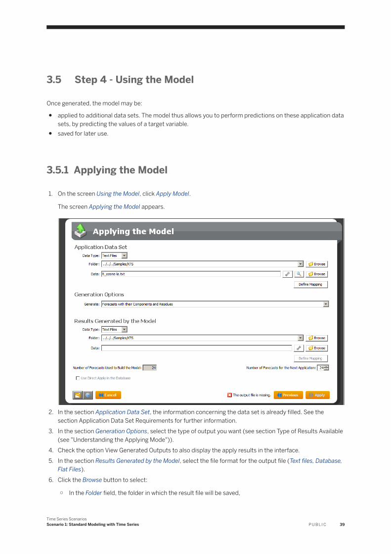
1. On the screen Using the Model, click Apply Model.

The screen Applying the Model appears.

2. In the section Application Data Set, the information concerning the data set is already filled. See the section Application Data Set Requirements for further information.

3. In the section Generation Options, select the type of output you want (see section Type of Results Available (see "Understanding the Applying Mode")).

4. Check the option View Generated Outputs to also display the apply results in the interface.5. In the section Results Generated by the Model, select the file format for the output file (Text files, Database,

Flat Files).6. Click the Browse button to select:

○ In the Folder field, the folder in which the result file will be saved,


○ In the Data field, the name of the result file.7. Click the Apply button.8. Click the Next button.

The screen Using the Model appears. Once application of the model has been completed, the results files of the application are automatically saved in the location that you had defined from the screen Applying the Model.

3.5.1.1 Application Data Set Requirements

The data set used to apply a time series model is generally the same used for training the model. Applying a time series model produces a similar output data set with extra columns and/or rows containing the requested forecasts.

It is also possible to apply a model to a different data set provided if the following conditions are fulfilled:

● the application data set must contain:○ the target variable.○ all the input variables from the training data set (that is, all the variables that have not been excluded

during the variables selection step).○ all the key variables from the training data set (except for the key variables automatically generated by

the application, such as KxIndex).● the date column must be sorted (strictly increasing, Order Level = 1 for ODBC sources).● the first date of the application data set must be present in the time window defining the training data set.

For example, for the ozone model, a data set ozone without the first 10 rows is a valid application data set while a data set starting with the date value ‘1973-03-01’ is not (since this date is not contained in the training data set, which ends on ‘1971-12-28’).

Type of Results Available

In the Generate pull-down menu you can choose to generate three types of results:

If you choose the option... The result file will contain...

Predicted Values Only ● all input variables,● the predicted variables, that is the forecasts for every

date of the training data set.

Forecasts with their Components ● all input variables,● the predicted variables, that is the forecasts for every

date of the training data set.● the components value (trend, cycles, fluctuation) for

each forecast



If you choose the option... The result file will contain...

Forecasts with their Components and Residues

● all input variables,● the predicted variables, that is the forecasts for every

date of the training data set.● the components value (trend, cycles, fluctuation) for

each forecast● the remaining values (residue) obtained after extracting

each component from each forecast

Only First Forecasts Column and their Error Bars

● all input variables,● the first predicted variable, that is the first forecast for

every date of the training data set.● the error bars for the predicted variable

3.5.1.2 Understanding the Application Mode

A time series model can only be applied on all or part of the training data set.

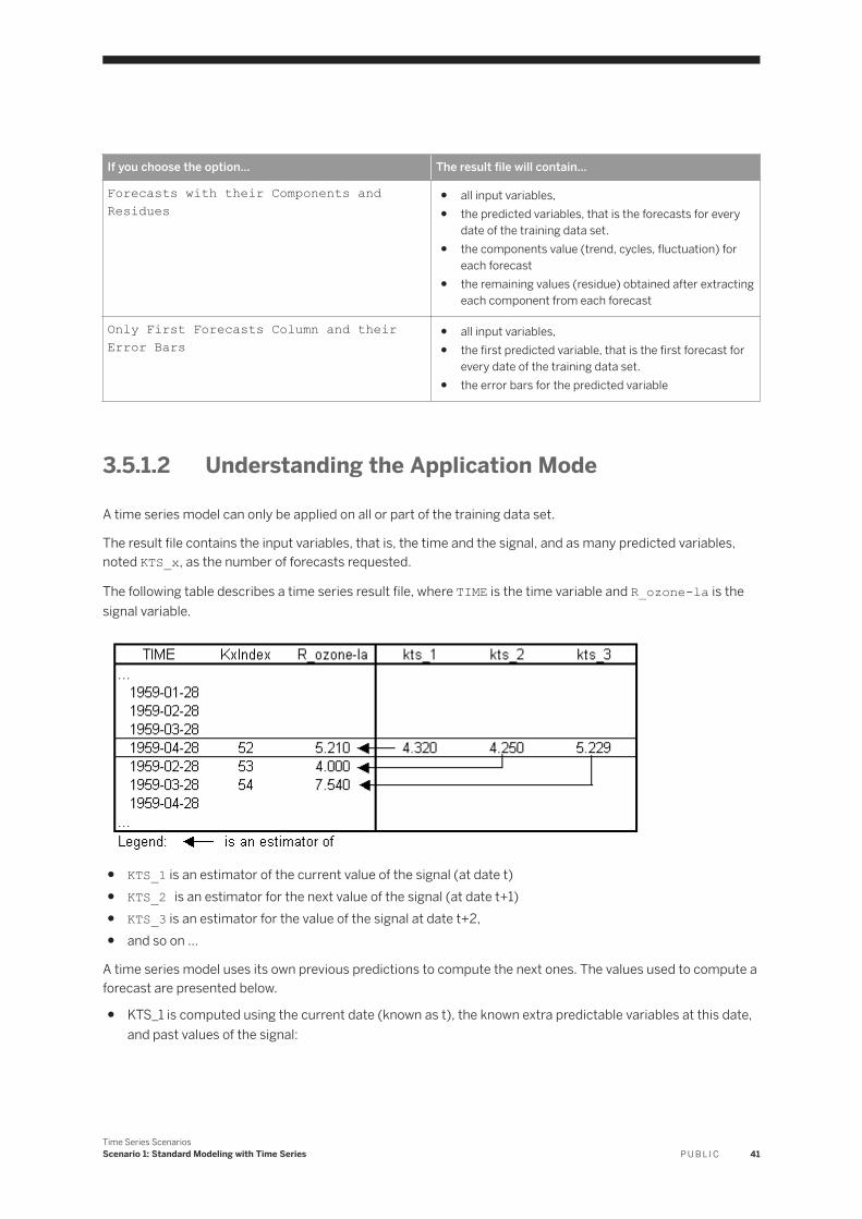
The result file contains the input variables, that is, the time and the signal, and as many predicted variables, noted KTS_x, as the number of forecasts requested.

The following table describes a time series result file, where TIME is the time variable and R_ozone-la is the signal variable.

● KTS_1 is an estimator of the current value of the signal (at date t)● KTS_2 is an estimator for the next value of the signal (at date t+1)● KTS_3 is an estimator for the value of the signal at date t+2,● and so on …

A time series model uses its own previous predictions to compute the next ones. The values used to compute a forecast are presented below.

● KTS_1 is computed using the current date (known as t), the known extra predictable variables at this date, and past values of the signal:


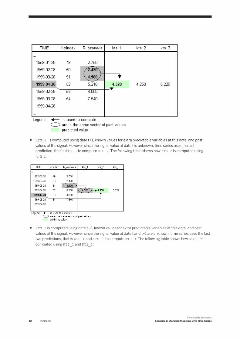
● KTS_2 is computed using date t+1, known values for extra predictable variables at this date, and past values of the signal. However since the signal value at date t is unknown, time series uses the last prediction, that is KTS_1, to compute KTS_2. The following table shows how KTS_2 is computed using KTS_1:

● KTS_3 is computed using date t+2, known values for extra predictable variables at this date, and past values of the signal. However since the signal value at date t and t+1 are unknown, time series uses the last two predictions, that is KTS_1 and KTS_2, to compute KTS_3. The following table shows how KTS_3 is computed using KTS_1 and KTS_2:



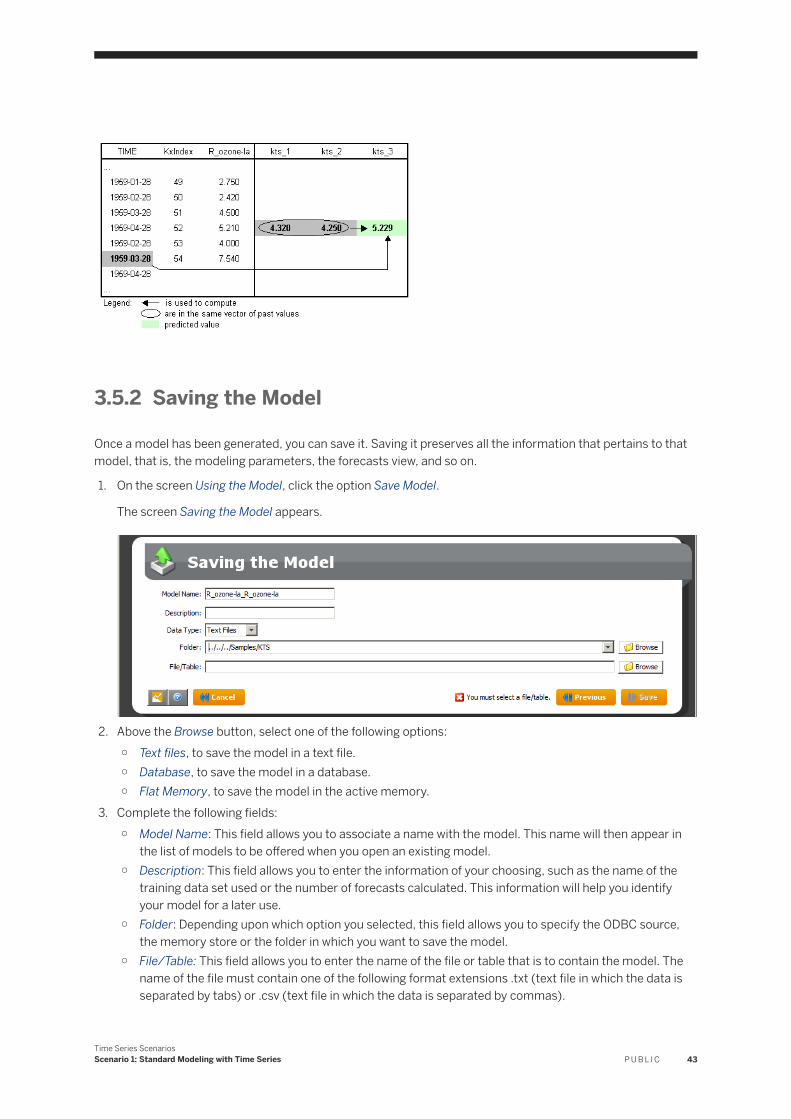
3.5.2 Saving the Model

Once a model has been generated, you can save it. Saving it preserves all the information that pertains to that model, that is, the modeling parameters, the forecasts view, and so on.

1. On the screen Using the Model, click the option Save Model.

The screen Saving the Model appears.

2. Above the Browse button, select one of the following options:○ Text files, to save the model in a text file.○ Database, to save the model in a database.○ Flat Memory, to save the model in the active memory.

3. Complete the following fields:○ Model Name: This field allows you to associate a name with the model. This name will then appear in

the list of models to be offered when you open an existing model.○ Description: This field allows you to enter the information of your choosing, such as the name of the

training data set used or the number of forecasts calculated. This information will help you identify your model for a later use.

○ Folder: Depending upon which option you selected, this field allows you to specify the ODBC source, the memory store or the folder in which you want to save the model.

○ File/Table: This field allows you to enter the name of the file or table that is to contain the model. The name of the file must contain one of the following format extensions .txt (text file in which the data is separated by tabs) or .csv (text file in which the data is separated by commas).


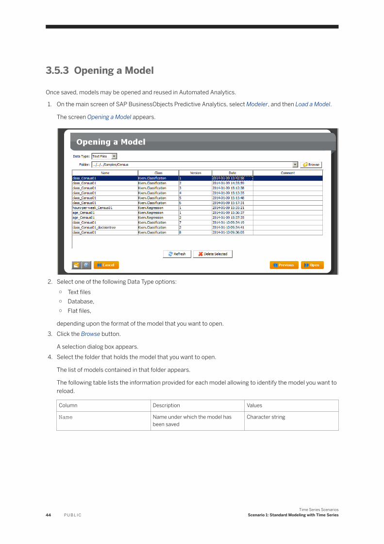
3.5.3 Opening a Model

Once saved, models may be opened and reused in Automated Analytics.

1. On the main screen of SAP BusinessObjects Predictive Analytics, select Modeler, and then Load a Model.

The screen Opening a Model appears.

2. Select one of the following Data Type options:○ Text files○ Database,○ Flat files,

depending upon the format of the model that you want to open.3. Click the Browse button.

A selection dialog box appears.4. Select the folder that holds the model that you want to open.

The list of models contained in that folder appears.

The following table lists the information provided for each model allowing to identify the model you want to reload.

Column Description Values

Name Name under which the model has been saved

Character string



Class Class of the model, that is the type of the model

○ Kxen.Classification: Classifica-tion/Regression with nominal target

○ Kxen.Regression: Classification/Regression with continuous target

○ Kxen.Segmentation : Clustering with SQL Mode

○ Kxen.Clustering : Clustering without SQL Mode

○ Kxen.TimeSeries: Time Series○ Kxen.AssociationRules: Associa

tion Rules○ Kxen.SimpleModel : Classifica-

tion/Regression and Clustering multi-target models, any other model

Version Number of the model version when the model has been saved several times

Integer starting at 1

Date Date when the model has been saved Date and time in the format yyyy-mm-dd hh:mm:ss

Comment Optional user defined comment that can be used to identify the model

Character string

5. Select a model from the list.6. Click the Open button.

The Using the Model menu appears.


4 Scenario 2: Modeling with Extra Predictable Variables

This section details:

● what are the extra inputs variables for time series,● how to use these extra variables,● what is the impact of this feature on the modeling.

4.1 Presentation

In Forecasting modeling, extra variables are exogenous factors that may have an influence on the modeling. These variables can be ordinal, binary or continuous.

These extra variables are Predictable variables as their future values are known (like the first Friday of the month, the first working day of the month, and so on). This type of variable can contain additional information, which can be very useful for the trend and/or the cyclic analysis.

The predictable variable is the subject of this section.

4.2 Standard Modeling

Summary of the Modeling Settings to Use

In this step, you will follow the default scenario without using any extras predictable variables (see section Standard Modeling with Time Series).

The table below summarizes the modeling settings that you must use. It should be sufficient for users who are already familiar with the KJWizard.

For detailed procedures and more information, see the following sections.

Replace the options given in the scenario by the following ones:

Task(s) Screen Settings

● Specifying the data source● Selecting a cutting strategy

Data to be Modeled ● In the field Data Set , select the file CashFlows.txt

● Cutting strategy : sequential without test


Scenario 2: Modeling with Extra Predictable Variables

Specifying a description file Data Description In the field Description , select the file KxDesc_CashFlows.txt

Defining the extra predictable inputs number

Selecting Variables Select and exclude all the variables from the field Predictable Variables Kept

Defining the Forecasts Number Summary of Modeling Parameters

In the field Number of Forecasts , enter 20

Selecting a Data Source and a Cutting Strategy

For this Scenario:

● Use the file CashFlows.txt as the training data set.● Select the cutting strategy Sequential without test.

For the detailed procedures, refer to sections Selecting a Data Source and Selecting a Cutting Strategy.

Describing the Data

For this Scenario, use the description file KxDesc_CashFlows.txt.

For the detailed procedure, refer to section Describing the Data Selected.

Selecting Variables

For this Scenario:

● Keep Date as the time variable.● Keep Cash as the target variable.● Exclude all extra predictable variables.● Do not select a weight variable.● Check that the last training line is set at 251.

On the screen Displaying the signal, select the option Date in the Time list.

For detailed procedures, refer to section Selecting Variables.

Defining the Forecasts Number

For this Scenario, define the number of forecasts to 21. This number corresponds to the average number of days worked in one month.

Time Series ScenariosScenario 2: Modeling with Extra Predictable Variables P U B L I C 47

For the detailed procedure, refer to section Defining the Number of Forecasts.

4.2.1 Viewing the Corresponding Forecasts

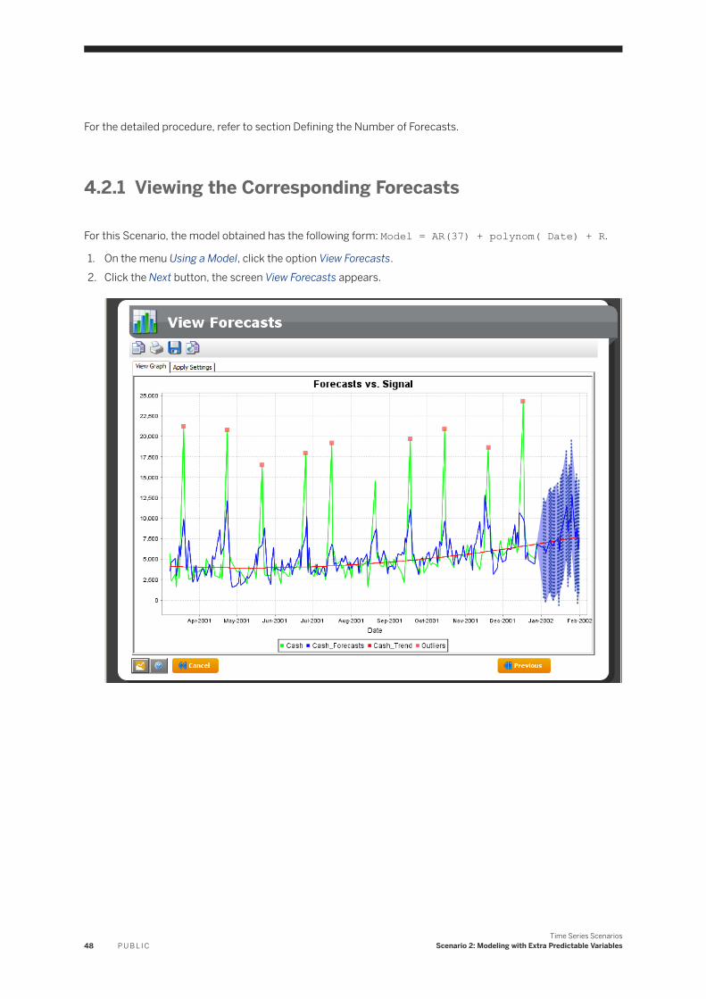
For this Scenario, the model obtained has the following form: Model = AR(37) + polynom( Date) + R.

1. On the menu Using a Model, click the option View Forecasts.2. Click the Next button, the screen View Forecasts appears.



4.3 Modeling with Extra Predictable Inputs

The following section will show how extra predictable variables can increase the performances on the current data set.

Summary of the Modeling Settings to Use

In this step, you will execute Scenario 2 using extra predictable variables. The table below summarizes the modeling settings that you must use. It should be sufficient enough for users who are already familiar with SAP BusinessObjects Predictive Analytics.

For detailed procedures and more information, see the following sections.

Replace the options given in the scenario by the following ones:

Task(s) Screen Settings

● Specifying the data source● Selecting a cutting strategy

Data to be Modeled ● In the field Data Set , select the file CashFlows.txt

● Cutting strategy : sequential without test

Specifying a description file Data Description • In the field Description , select the file KxDesc_CashFlows.txt

Defining the extra predictable inputs Selecting Variables • Keep all the variables in the field Predictable Variables Kept

Defining the Forecasts Number Summary of Modeling Parameters • In the field Number of Forecasts , enter 21

Selecting a Cutting Strategy and a Data Source

For this Scenario:

● Use the file CashFlows.txt as the training data set.● Select the cutting strategy Sequential without test.

For the detailed procedures, refer to sections Selecting a Data Source and Selecting a Cutting Strategy.

Describing the Data

For this Scenario, use the description file KxDesc_CashFlows.txt.

For the detailed procedure, refer to section Describing the Data Selected.


Selecting Variables

The panel Selecting Variables allows you to:

● select the time variable,● select the target variable,● select a weight variable (optional),● set the last date to use for training the model,● select which variables should be kept for the modeling.

For this Scenario:

● Keep Date as the time variable.● Keep Cash as the target variable.● Keep all the extra predictable variables.● Do not select a weight variable.● Check that the last training line is set at 251.

On the screen Displaying the Signal:

● Select the option Date in the Time list.

For the detailed procedures, refer to section Selecting Variables.

Defining the Forecasts Number

For this Scenario, define the number of forecasts to 21. This number corresponds to the average number of days worked in one month.

For the detailed procedure, refer to section Defining the Number of Forecasts.

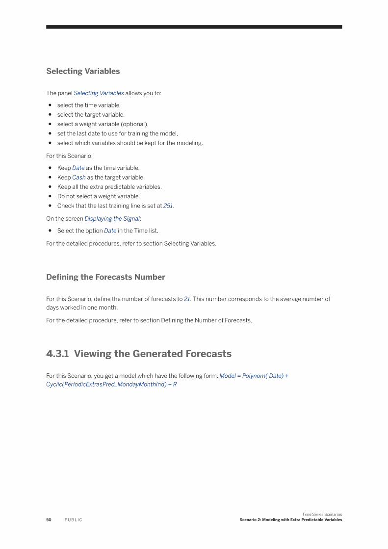
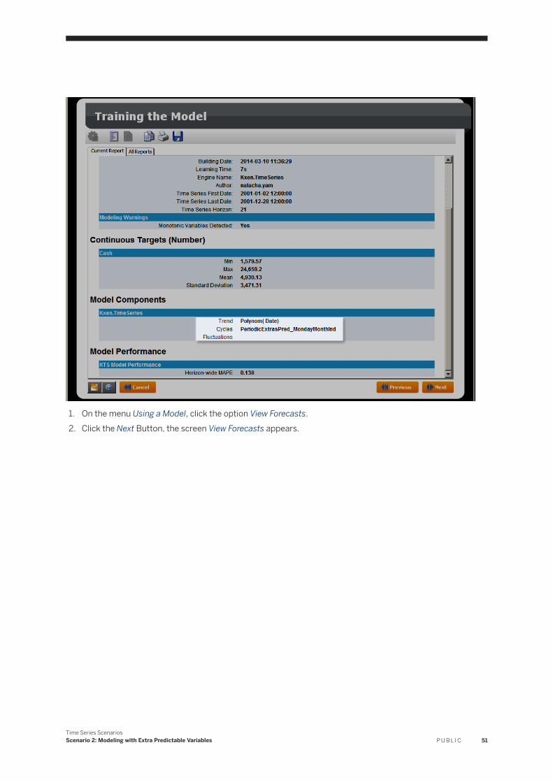
4.3.1 Viewing the Generated Forecasts

For this Scenario, you get a model which have the following form: Model = Polynom( Date) + Cyclic(PeriodicExtrasPred_MondayMonthInd) + R



1. On the menu Using a Model, click the option View Forecasts.2. Click the Next Button, the screen View Forecasts appears.


4.4 Comparing the Forecasts With and Without Extra Predictable Variables

To better understand how extra predictable variables can improve a model, this section will analyze and compare the forecasts obtained with both a standard modeling and a modeling with extra predictable variables.

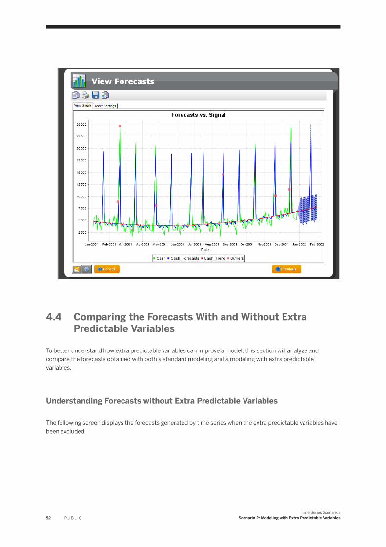
Understanding Forecasts without Extra Predictable Variables

The following screen displays the forecasts generated by time series when the extra predictable variables have been excluded.



In this model, the engine uses its own variables (cyclics, trend, fluctuations,...) to generate the more predictive model possible. The trend and the picks position are correctly detected but the following points could be improved:

● the error bars are very extended, meaning that the confidence of the model is low,● the picks amplitude is not correctly forecasted,● the model appears noisy.

The solution to refine this model is to add extra predictable variables.

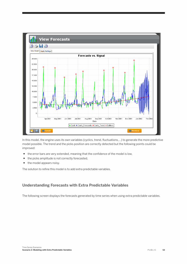
Understanding Forecasts with Extra Predictable Variables

The following screen displays the forecasts generated by time series when using extra predictable variables.


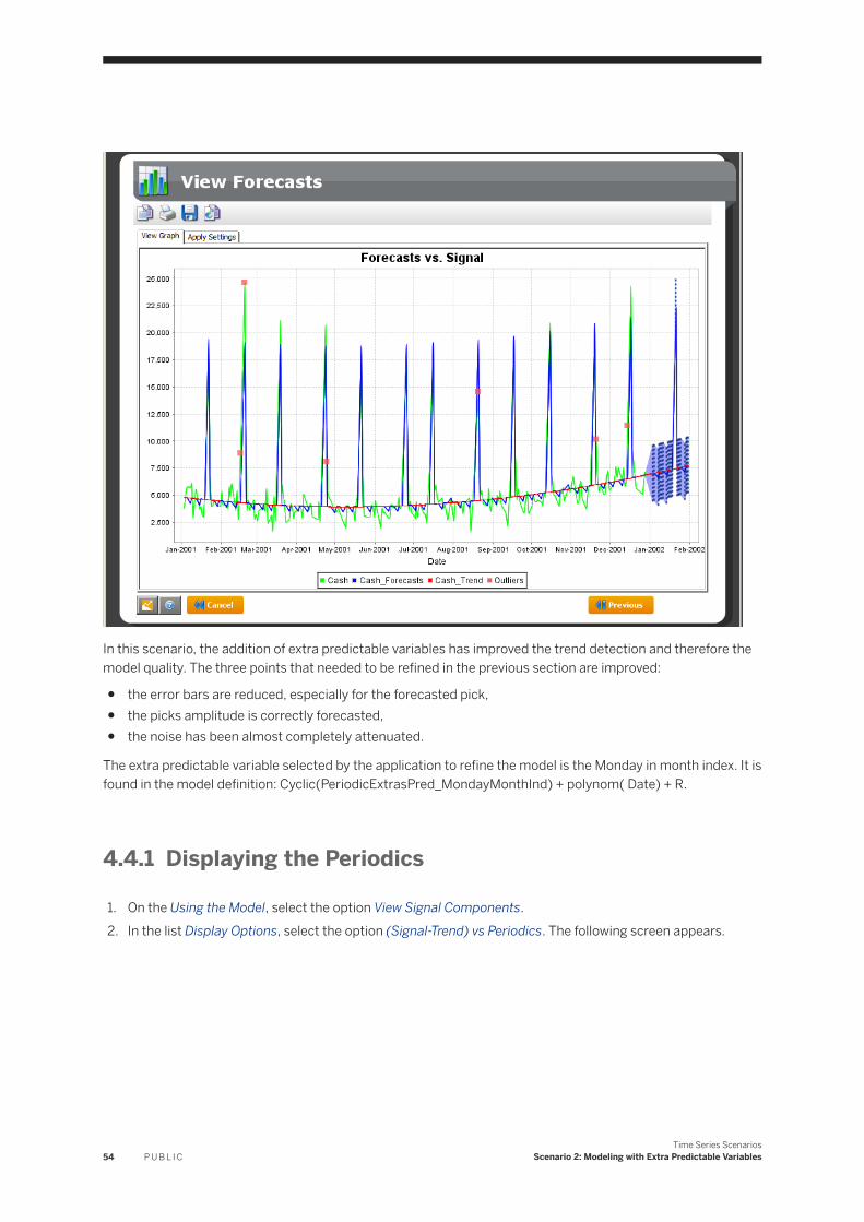
In this scenario, the addition of extra predictable variables has improved the trend detection and therefore the model quality. The three points that needed to be refined in the previous section are improved:

● the error bars are reduced, especially for the forecasted pick,● the picks amplitude is correctly forecasted,● the noise has been almost completely attenuated.

The extra predictable variable selected by the application to refine the model is the Monday in month index. It is found in the model definition: Cyclic(PeriodicExtrasPred_MondayMonthInd) + polynom( Date) + R.

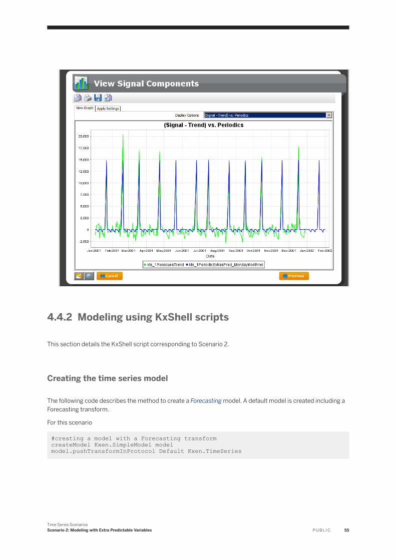
4.4.1 Displaying the Periodics

1. On the Using the Model, select the option View Signal Components.2. In the list Display Options, select the option (Signal-Trend) vs Periodics. The following screen appears.



4.4.2 Modeling using KxShell scripts

This section details the KxShell script corresponding to Scenario 2.

Creating the time series model

The following code describes the method to create a Forecasting model. A default model is created including a Forecasting transform.

For this scenario

#creating a model with a Forecasting transform createModel Kxen.SimpleModel model model.pushTransformInProtocol Default Kxen.TimeSeries


Setting the model parameters

The cutting strategy is the only one model parameter, which has to be set.

For this scenario

#setting the model’s parameters model.getParameter ""model.changeParameter "Parameters/CutTrainingPolicy" "sequential with no test"model.validateParameter

Opening the Training Data Set

In this step, the training data set CashFlows.txt is opened with its description KxDesc_CashFlows.txt. As the file contains training information and predictive information, the line index of the end of training is fixed.

For this scenario

#open the training data set model.openNewStore Kxen.FileStore .model.newDataSet Training CashFlows.txt model.readSpaceDescription Training KxDesc_CashFlows.txt

#set the line index of the end of training bind model DataSet Training myDatasetmyDataset.getParameter ""myDataset.changeParameter "Parameters/LastRow" 251myDataset.validateParameter delete myDataset

4.4.2.1 Setting the time series transform parameter

The Forecasting transform parameters are the following:

● AutoFeedCount saves the number of forecasts asked by the user (default = 1).● MaxCyclics indicates the maximum number of cyclicalities, that will be analyzed by time series (default =

450).● DateColumnName saves the name of the date variable (required parameter).● ForecastsConnection gives the format of the forecasts in the output of time series (default = 1). If its value

is 1, then the forecasts will be transposed at the end of the KTS_1 variable with the corresponding dates. If its value is 0, then the forecasts stay in the last line of the file.

● LastRowWithForecastingInformation saves the index of the last line of the file. This parameter is required if you want to use extras predictable inputs.

● PredictableExtras saves the names of the extras predictable variable.● ExtraMode, gives the the format of the output of time series (default = No Extra). <No Extra> value is the

default format with the KTS_ variables. <Signal Components> value is the format which includes with the previous cited variables, each component of each variables: trend, cycles/seasonality, fluctuations.



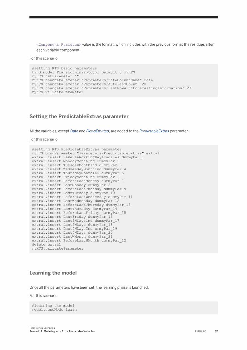
<Component Residues> value is the format, which includes with the previous format the residues after each variable component.

For this scenario

#setting KTS basic parameters bind model TransformInProtocol Default 0 myKTSmyKTS.getParameter ""myKTS.changeParameter "Parameters/DateColumnName" DatemyKTS.changeParameter "Parameters/AutoFeedCount" 20myKTS.changeParameter "Parameters/LastRowWithForecastingInformation" 271myKTS.validateParameter

Setting the PredictableExtras parameter

All the variables, except Date and FlowsEmitted, are added to the PredictableExtras parameter.

For this scenario

#setting KTS PredictableExtras parameter myKTS.bindParameter "Parameters/PredictableExtras" extra1extra1.insert ReverseWorkingDaysIndices dummyPar_1extra1.insert MondayMonthInd dummyPar_2extra1.insert TuesdayMonthInd dummyPar_3extra1.insert WednesdayMonthInd dummyPar_4extra1.insert ThursdayMonthInd dummyPar_5extra1.insert FridayMonthInd dummyPar_6extra1.insert BeforeLastMonday dummyPar_7extra1.insert LastMonday dummyPar_8extra1.insert BeforeLastTuesday dummyPar_9extra1.insert LastTuesday dummyPar_10extra1.insert BeforeLastWednesday dummyPar_11extra1.insert LastWednesday dummyPar_12extra1.insert BeforeLastThursday dummyPar_13extra1.insert LastThursday dummyPar_14extra1.insert BeforeLastFriday dummyPar_15extra1.insert LastFriday dummyPar_16extra1.insert Last5WDaysInd dummyPar_17extra1.insert Last5WDays dummyPar_18extra1.insert Last4WDaysInd ummyPar_19extra1.insert Last4WDays dummyPar_20extra1.insert LastWMonth dummyPar_21extra1.insert BeforeLastWMonth dummyPar_22delete extra1 myKTS.validateParameter

Learning the model

Once all the parameters have been set, the learning phase is launched.

For this scenario

#learning the model model.sendMode learn


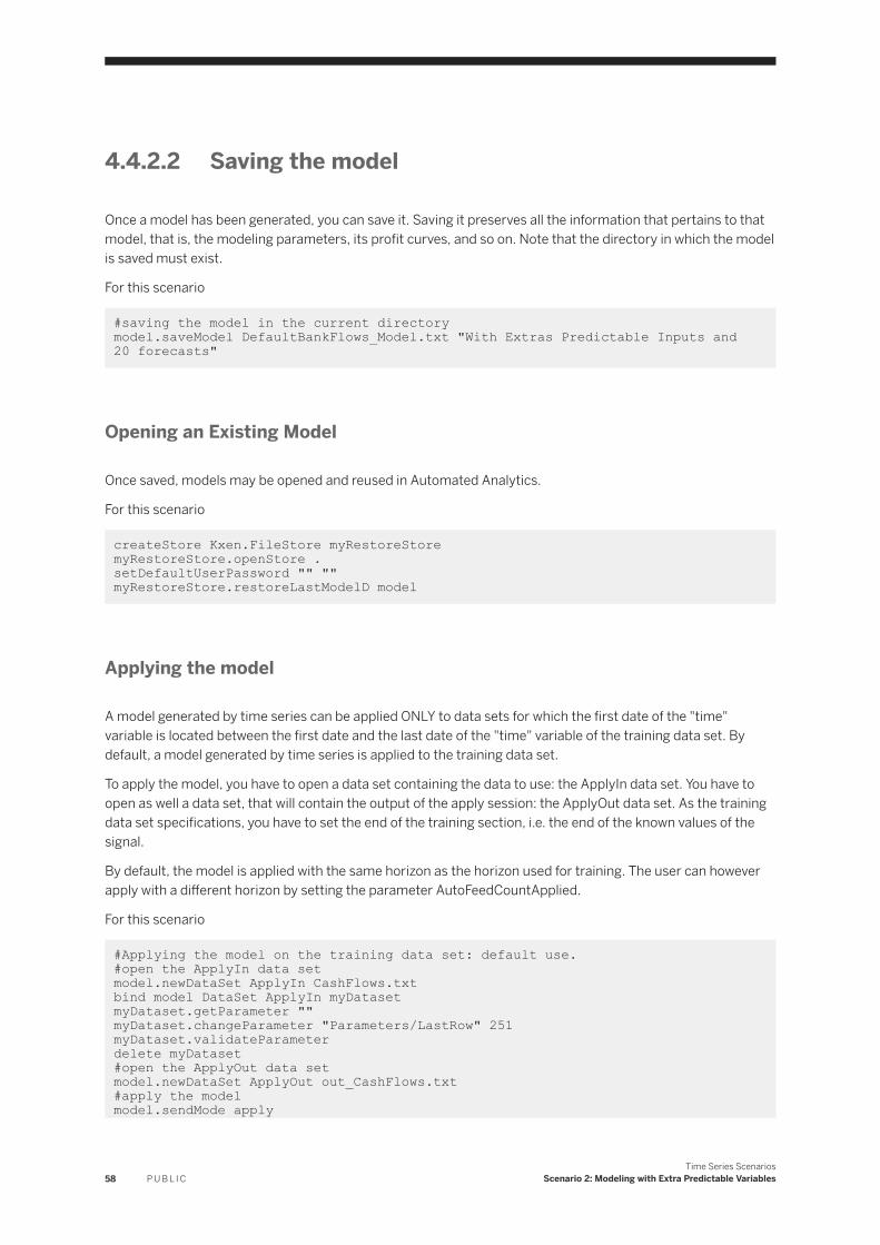
4.4.2.2 Saving the model

Once a model has been generated, you can save it. Saving it preserves all the information that pertains to that model, that is, the modeling parameters, its profit curves, and so on. Note that the directory in which the model is saved must exist.

For this scenario

#saving the model in the current directory model.saveModel DefaultBankFlows_Model.txt "With Extras Predictable Inputs and 20 forecasts"

Opening an Existing Model

Once saved, models may be opened and reused in Automated Analytics.

For this scenario

createStore Kxen.FileStore myRestoreStore myRestoreStore.openStore .setDefaultUserPassword "" "" myRestoreStore.restoreLastModelD model

Applying the model

A model generated by time series can be applied ONLY to data sets for which the first date of the "time" variable is located between the first date and the last date of the "time" variable of the training data set. By default, a model generated by time series is applied to the training data set.

To apply the model, you have to open a data set containing the data to use: the ApplyIn data set. You have to open as well a data set, that will contain the output of the apply session: the ApplyOut data set. As the training data set specifications, you have to set the end of the training section, i.e. the end of the known values of the signal.

By default, the model is applied with the same horizon as the horizon used for training. The user can however apply with a different horizon by setting the parameter AutoFeedCountApplied.

For this scenario

#Applying the model on the training data set: default use. #open the ApplyIn data setmodel.newDataSet ApplyIn CashFlows.txtbind model DataSet ApplyIn myDatasetmyDataset.getParameter ""myDataset.changeParameter "Parameters/LastRow" 251myDataset.validateParameterdelete myDataset#open the ApplyOut data setmodel.newDataSet ApplyOut out_CashFlows.txt#apply the modelmodel.sendMode apply



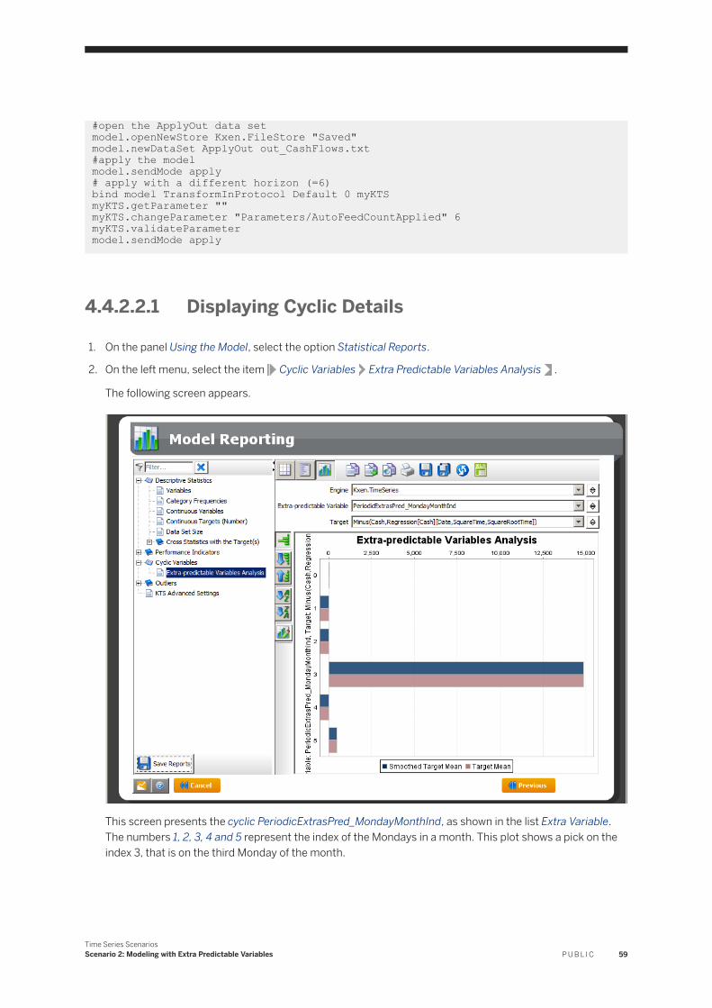
#open the ApplyOut data setmodel.openNewStore Kxen.FileStore "Saved"model.newDataSet ApplyOut out_CashFlows.txt #apply the modelmodel.sendMode apply# apply with a different horizon (=6)bind model TransformInProtocol Default 0 myKTSmyKTS.getParameter ""myKTS.changeParameter "Parameters/AutoFeedCountApplied" 6myKTS.validateParametermodel.sendMode apply

4.4.2.2.1 Displaying Cyclic Details

1. On the panel Using the Model, select the option Statistical Reports.

2. On the left menu, select the item Cyclic Variables Extra Predictable Variables Analysis .

The following screen appears.

This screen presents the cyclic PeriodicExtrasPred_MondayMonthInd, as shown in the list Extra Variable. The numbers 1, 2, 3, 4 and 5 represent the index of the Mondays in a month. This plot shows a pick on the index 3, that is on the third Monday of the month.


Important Disclaimers and Legal Information

Coding SamplesAny software coding and/or code lines / strings ("Code") included in this documentation are only examples and are not intended to be used in a productive system environment. The Code is only intended to better explain and visualize the syntax and phrasing rules of certain coding. SAP does not warrant the correctness and completeness of the Code given herein, and SAP shall not be liable for errors or damages caused by the usage of the Code, unless damages were caused by SAP intentionally or by SAP's gross negligence.

AccessibilityThe information contained in the SAP documentation represents SAP's current view of accessibility criteria as of the date of publication; it is in no way intended to be a binding guideline on how to ensure accessibility of software products. SAP in particular disclaims any liability in relation to this document. This disclaimer, however, does not apply in cases of willful misconduct or gross negligence of SAP. Furthermore, this document does not result in any direct or indirect contractual obligations of SAP.

Gender-Neutral LanguageAs far as possible, SAP documentation is gender neutral. Depending on the context, the reader is addressed directly with "you", or a gender-neutral noun (such as "sales person" or "working days") is used. If when referring to members of both sexes, however, the third-person singular cannot be avoided or a gender-neutral noun does not exist, SAP reserves the right to use the masculine form of the noun and pronoun. This is to ensure that the documentation remains comprehensible.

Internet HyperlinksThe SAP documentation may contain hyperlinks to the Internet. These hyperlinks are intended to serve as a hint about where to find related information. SAP does not warrant the availability and correctness of this related information or the ability of this information to serve a particular purpose. SAP shall not be liable for any damages caused by the use of related information unless damages have been caused by SAP's gross negligence or willful misconduct. All links are categorized for transparency (see: http://help.sap.com/disclaimer).


Important Disclaimers and Legal Information

http://help.sap.com/disclaimer/

Time Series ScenariosImportant Disclaimers and Legal Information P U B L I C 61

go.sap.com/registration/contact.html

© 2017 SAP SE or an SAP affiliate company. All rights reserved.No part of this publication may be reproduced or transmitted in any form or for any purpose without the express permission of SAP SE or an SAP affiliate company. The information contained herein may be changed without prior notice.Some software products marketed by SAP SE and its distributors contain proprietary software components of other software vendors. National product specifications may vary.These materials are provided by SAP SE or an SAP affiliate company for informational purposes only, without representation or warranty of any kind, and SAP or its affiliated companies shall not be liable for errors or omissions with respect to the materials. The only warranties for SAP or SAP affiliate company products and services are those that are set forth in the express warranty statements accompanying such products and services, if any. Nothing herein should be construed as constituting an additional warranty.SAP and other SAP products and services mentioned herein as well as their respective logos are trademarks or registered trademarks of SAP SE (or an SAP affiliate company) in Germany and other countries. All other product and service names mentioned are the trademarks of their respective companies.Please see http://www.sap.com/corporate-en/legal/copyright/index.epx for additional trademark information and notices.

https://go.sap.com/registration/contact.html

https://go.sap.com/registration/contact.html

http://www.sap.com/corporate-en/legal/copyright/index.epx

http://www.sap.com/corporate-en/legal/copyright/index.epx

Time Series Scenarios - SAP · PDF filePUBLIC SAP BusinessObjects Predictive Analytics 3.1 2017-10-26 Time Series Scenarios Automated Analytics User Guide

Documents