Time-series modelling of aggregate wind power output

Time-series modelling of aggregate wind power output

Alexander Sturt, Goran Strbac17 March 2011

Introduction

Eastern Wind Integration and Transmission Study (EWITS) (2010)

• Wind datasets prepared by AWS Truewind over 9 month period

• Created by simulation using mesoscale Numerical Weather Prediction (NWP) model

• 3 years of synthetic data, 1326 sites (freely available online)

• Hardware used: 80 x dual CPU quad core penguin workstations (640 cores)

• Run time per year of simulation: 21 days (in theory...)

What if this level of detail isn’t needed?What if we need a model of aggregated wind output?What if we need to understand the statistical properties?

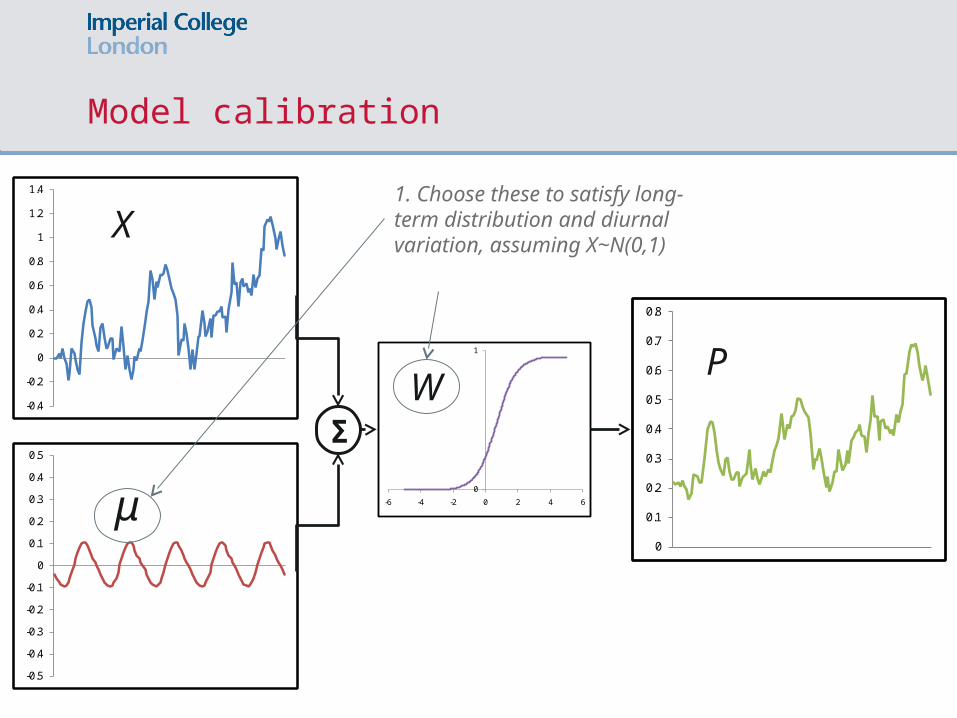
Modelling strategy

• Univariate model for aggregate wind power, not wind speed• Autoregressive driver: AR(p), hourly (or half-hourly) timesteps

• Include diurnal variation with periodic additive term:

• Fit to long-term distribution with transformation function:

• Use different models for the different seasons

kkkk XXX ...2211 iid N(0,1)

nkkk XX mod

kk XP W

n = number of data points per day

Model calibration

-0.4

-0.2

0

0.2

0.4

0.6

0.8

1

1.2

1.4

-0.5

-0.4

-0.3

-0.2

-0.1

0

0.1

0.2

0.3

0.4

0.5

0

1

-6 -4 -2 0 2 4 6

0

0.1

0.2

0.3

0.4

0.5

0.6

0.7

0.8

Σ

X

μ

WP

1. Choose these to satisfy long-term distribution and diurnal variation, assuming X~N(0,1)

Model calibration

-0.4

-0.2

0

0.2

0.4

0.6

0.8

1

1.2

1.4

-0.5

-0.4

-0.3

-0.2

-0.1

0

0.1

0.2

0.3

0.4

0.5

0

1

-6 -4 -2 0 2 4 6

0

0.1

0.2

0.3

0.4

0.5

0.6

0.7

0.8

Σ

X

μ

WP

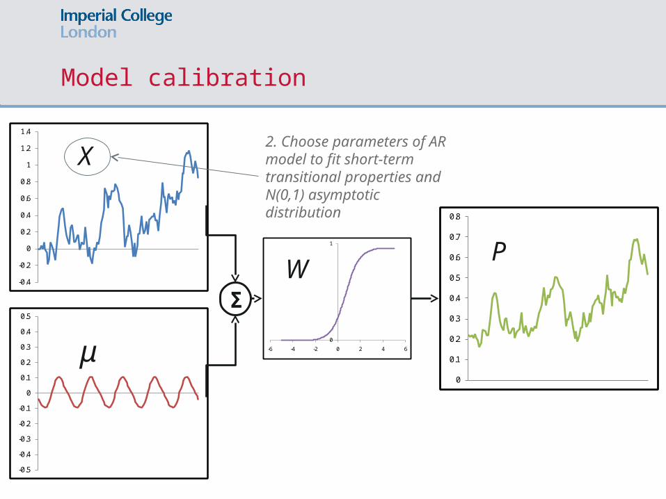
2. Choose parameters of AR model to fit short-term transitional properties and N(0,1) asymptotic distribution

Case study: GB2030 model

• 6 years of hourly wind speed data taken from MIDAS dataset by Olmos (2009)

• 116 sites (onshore only)• 10m anemometer data extrapolated to hub-height and

converted to wind power using turbine curve• Regional weightings chosen to match core 2030 buildout

scenario used by Poyry (2009); offshore capacity mapped to nearest onshore regions

Olmos Poyry

GB2030: modelling strategy

• Weighted regional power output aggregated to produce a univariate time series

• Split into four seasons• For each season, calibrate model to reproduce

asymptotic distribution, diurnal variation and short-term volatility, using AR(2) model

• Tweak to approximate effect of offshore component

GB2030 (untweaked): distribution and volatility

0

200

400

600

800

1000

1200

1400

1600

1800

0-0.

050.

05-0

.10.

1-0.

150.

15-0

.20.

2-0.

250.

25-0

.30.

3-0.

350.

35-0

.40.

4-0.

450.

45-0

.50.

5-0.

550.

55-0

.60.

6-0.

650.

65-0

.70.

7-0.

750.

75-0

.80.

8-0.

850.

85-0

.90.

9-0.

950.

95-1

Occ

urre

nces

per

yea

r

Power output bucket (p.u.)

Sim Upper Sim LowerSim Mean Hist2001-2Hist2002-3 Hist2003-4Hist2004-5 Hist2005-6Hist2006-7 Hist Av

0.00

0.05

0.10

0.15

0.20

0.25

0 5 10 15 20

RMS

chan

ge (p

.u.)

Time horizon (hr)

Sim Upper Sim LowerSim Mean Hist2001-2Hist2002-3 Hist2003-4Hist2004-5 Hist2005-6Hist2006-7 HistAv

Power output distribution Volatility curve

GB2030 (untweaked):distribution of absolute power output changes

0.01

0.1

1

10

100

1000

10000

0-0.

05

0.05

-0.1

0.1-

0.15

0.15

-0.2

0.2-

0.25

0.25

-0.3

Occ

urre

nces

per

yea

r

Power output change bucket (p.u.)


0.01

0.1

1

10

100

1000

10000

0-0.

05

0.05

-0.1

0.1-

0.15

0.15

-0.2

0.2-

0.25

0.25

-0.3

0.3-

0.35

0.35

-0.4

0.4-

0.45

0.45

-0.5

0.5-

0.55

0.55

-0.6

0.6-

0.65

Occ

urre

nces

per

yea

r



0.01

0.1

1

10

100

1000

10000

0-0.

05

0.05

-0.1

0.1-

0.15

0.15

-0.2

0.2-

0.25

0.25

-0.3

0.3-

0.35

0.35

-0.4

0.4-

0.45

0.45

-0.5

0.5-

0.55

0.55

-0.6

0.6-

0.65

0.65

-0.7

0.7-

0.75

0.75

-0.8

Occ

urre

nces

per

yea

r



0.01

0.1

1

10

100

1000

10000

0-0.

050.

05-0

.10.

1-0.

150.

15-0

.20.

2-0.

250.

25-0

.30.

3-0.

350.

35-0

.40.

4-0.

450.

45-0

.50.

5-0.

550.

55-0

.60.

6-0.

650.

65-0

.70.

7-0.

750.

75-0

.80.

8-0.

850.

85-0

.90.

9-0.

95

Occ

urre

nces

per

yea

r



1 hr 4 hr

8 hr 24 hr

GB2030: variation of 4hr volatility with power level

0

0.02

0.04

0.06

0.08

0.1

0.12

0.14

0.16

0.18

0.2

0-0.

1

0.1-

0.2

0.2-

0.3

0.3-

0.4

0.4-

0.5

0.5-

0.6

0.6-

0.7

0.7-

0.8

0.8-

0.9

0.9-

1.0

Mea

n ab

solu

te ch

ange

(p.u

.)



0

1

-6 -4 -2 0 2 4 6

W(x)

x

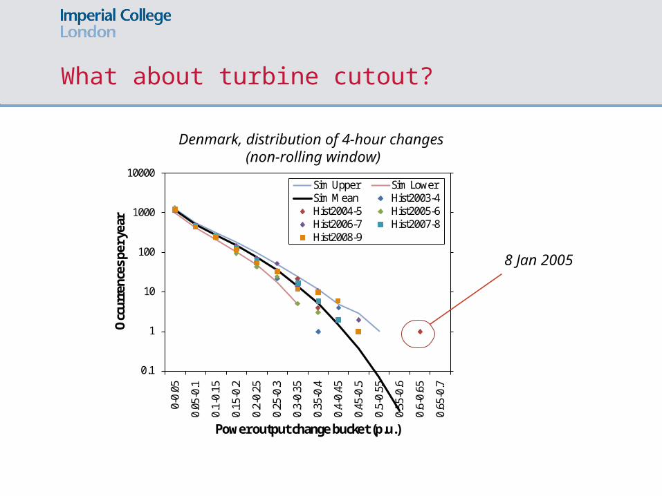
What about turbine cutout?

0.1

1

10

100

1000

100000-

0.05

0.05

-0.1

0.1-

0.15

0.15

-0.2

0.2-

0.25

0.25

-0.3

0.3-

0.35

0.35

-0.4

0.4-

0.45

0.45

-0.5

0.5-

0.55

0.55

-0.6

0.6-

0.65

0.65

-0.7

Occ

urre

nces

per

yea

r


Sim Upper Sim LowerSim Mean Hist2003-4Hist2004-5 Hist2005-6Hist2006-7 Hist2007-8Hist2008-9

8 Jan 2005

Denmark, distribution of 4-hour changes (non-rolling window)

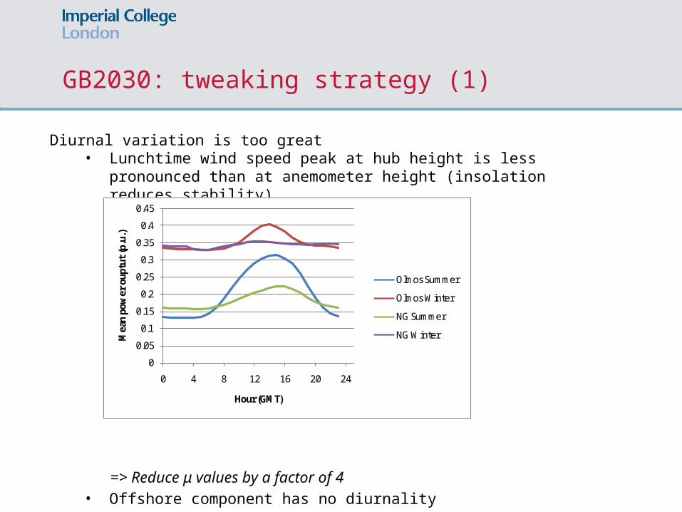
GB2030: tweaking strategy (1)

Diurnal variation is too great• Lunchtime wind speed peak at hub height is less pronounced

than at anemometer height (insolation reduces stability)

• Offshore component has no diurnality

0

0.05

0.1

0.15

0.2

0.25

0.3

0.35

0.4

0.45

0 4 8 12 16 20 24

Mea

n po

wer

oup

tut

(p.u

.)

Hour (GMT)

Olmos Summer

Olmos Winter

NG Summer

NG Winter

=> Reduce μ values by a factor of 4

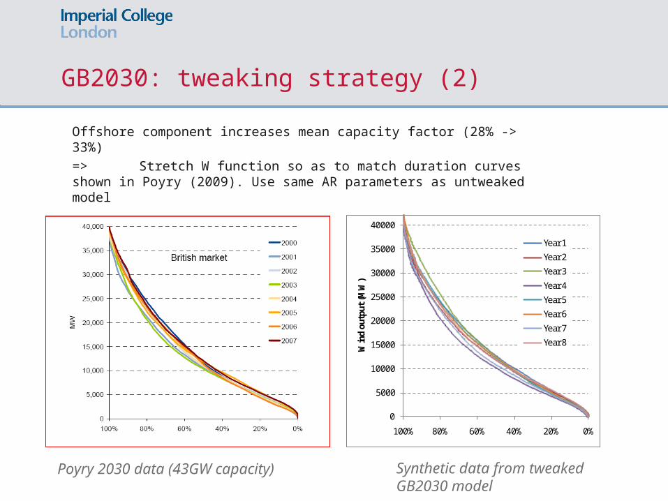
GB2030: tweaking strategy (2)

Offshore component increases mean capacity factor (28% -> 33%)=> Stretch W function so as to match duration curves shown in Poyry (2009). Use same AR parameters as untweaked model

0

5000

10000

15000

20000

25000

30000

35000

40000

0%20%40%60%80%100%

Win

d ou

tput

(MW

)

Year 1

Year 2

Year 3

Year 4

Year 5

Year 6

Year 7

Year 8

Poyry 2030 data (43GW capacity) Synthetic data from tweaked GB2030 model

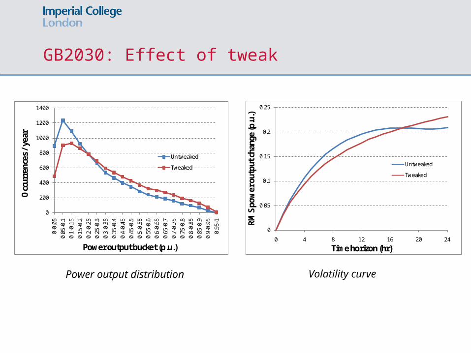
GB2030: Effect of tweak

0

0.05

0.1

0.15

0.2

0.25

0 4 8 12 16 20 24

RMS

pow

er o

utpu

t cha

nge

(p.u

.)Time horizon (hr)

Untweaked

Tweaked

Power output distribution Volatility curve

0

200

400

600

800

1000

1200

1400

0-0.

050.

05-0

.10.

1-0.

150.

15-0

.20.

2-0.

250.

25-0

.30.

3-0.

350.

35-0

.40.

4-0.

450.

45-0

.50.

5-0.

550.

55-0

.60.

6-0.

650.

65-0

.70.

7-0.

750.

75-0

.80.

8-0.

850.

85-0

.90.

9-0.

950.

95-1

Occ

urre

nces

/ y

ear


Untweaked

Tweaked

0

5

10

15

20

25

30

35

40

45

01-Dec-08 11-Dec-08 21-Dec-08 31-Dec-08 10-Jan-09 20-Jan-09 30-Jan-09

Win

d ou

tput

(GW

)GB2030: Time history sample (“Turing test”)

Win

d o

utp

ut

(GW

)

Poyry data

Tweaked GB2030 synthetic winter data

• Non-Gaussian wind power time series can be transformed to a Gaussian (X) domain and modelled with a Gaussian time series model

• Synthetic time series reproduce the important long-term and transitional properties (for power system simulation)

• Simplicity of model makes it possible to write down formulae for any desired statistic

• Transformation to Gaussian domain simplifies modelling of correlated RVs:

• Forecast errors (anti-correlated with wind realisation to prevent forecast biasing)

• Multi-bus models• Combined demand / wind model

Conclusions

• Sturt, A. and Strbac, G. “Time series modelling of power output for large-scale wind fleets”, Wind Energy, 2011 (to be published)

• Enernex Corporation “Eastern Wind Integration and Transmission Study”, 2010 http://www.nrel.gov/wind/systemsintegration/ewits.html

• Olmos, P. “Probability distribution of wind power during peak demand”, MSc dissertation, University of Edinburgh, 2009

• Olmos, P.E., Dent, C., Harrison, G.P. and Bialek, J.W. “Realistic calculation of wind generation capacity credits”, CIGRE/IEEE Symposium on integration of wide-scale renewable resources into the power delivery system, Calgary, 2009

• Poyry Energy Consulting, “Impact of intermittency: how wind variability could change the shape of the British and Irish electricity markets: summary report”, 2009 http://www.poyry.com

• Sturt, A. and Strbac, G. “A time series model for the aggregate GB wind output circa 2030”, 2011http://www.ee.ic.ac.uk/%20alexander.sturt07/GB2030SOM.pdf

References

http://www.nrel.gov/wind/systemsintegration/ewits.html



http://www.poyry.com/

http://www.ee.ic.ac.uk/%20alexander.sturt07/GB2030SOM.pdf

Time-series modelling of aggregate wind power output

Documents

wind datasets

diurnal variation

power levelwxxwhat

longterm distribution

model calibrationxwp2

parameters of ar model

greatlunchtime wind

years of synthetic data