Time Series Modeling with Hidden Variables and Gradient ...

Time Series Modeling

with Hidden Variables

and Gradient-Based Algorithms

by

Piotr Mirowski

A dissertation submitted in partial fulfillment

of the requirements for the degree of

Doctor of Philosophy

Department of Computer Science

Courant Institute of Mathematical Sciences

New York University

January, 2011

Yann LeCun

c© Piotr Mirowski

All Rights Reserved, 2011

In memory of Sam Roweis,

who laid the foundations

for this research

iii

Acknowledgements

These past five and a half years of doctoral studies at New York University have

constituted a personally transformative experience (and I am claiming this indepen-

dently of the jazz clubs, concert halls and vibrant community populating the greater

Greenwich Village area). During these years, I have benefited from countless con-

tributions that are impossible to acknowledge in a few lines. I will limit myself to

mentioning a few individuals who directly enabled this work, hoping to eventually

have the opportunity to contribute to someone else’s development in return.

I would like to immensely thank my adviser, Prof. Yann LeCun, for providing me

with resources, guidance, and freedom to pursue my research. Merci beaucoup pour

avoir cru en moi, Yann. Yann LeCun’s lab is an intellectual hub with connections

far beyond the field of Machine Learning, and therefore a very exciting research

environment. Pursuing there my doctoral work has provided me with a constant

source of instructive interactions. On a personal level, I admire Yann’s wide range

of musical, robotic, political, culinary and cultural interests as well as his ability to

convert extremely complex mathematics and neuroscience into tangible and intuitive

concepts in order to build things. I also greatly appreciate his “open door” policy

that enabled us to discuss research for long hours and that sustained my motivation

in the darkest hours of debugging.

The development of the techniques described in this doctoral work and the need

for proofs of concept were only a pretext to start highly stimulating collaborations

and to discover amazing researchers and specialists in fields I cannot comprehend. I

will begin with Dr. Ruben Kuzniecky and Dr. Deepak Madhavan, who originated

my research on the prediction of epileptic seizures from EEG and who provided me

with three semesters and two summers of funding through NYU’s FACES (Finding A

iv

Cure for Epilepsy and Seizures) foundation. Thanks to them, I learned the patient’s

perspective on the statistical concepts of “false positive” and “false negative”. Still in

the field of epilepsy prediction, I would also like to acknowledge fruitful discussions

with Profs Nandor Ludvig, Sertac Artan and Thomas Thesen.

Second, I am very grateful to Prof. Dennis Shasha, for providing me with a difficult

and defining problem for my doctoral studies, with an application to Computational

Biology. Dennis Shasha invested a lot of time and attention in my research, supporting

my many endeavors and professional aspirations, and effectively making me a member

of his lab and of the NYU Center for Genomics and Systems Biology. Along with

Gabriel Krouk, who tried to teach me genetics, and with Jesse Lingeman, we made a

fine team with whom I would like to maintain close ties.

Third, I would like to thank Craig Friedman from Standard & Poor’s, who pro-

vided me with precious feedback, intellectual stimulation, statistical rigour and sum-

mer support for my work on sentiment analysis and text categorization, and who

sparked my research interest in dynamic topic modeling.

And last but not least among the external collaborations, I am very grateful to

Sumit Chopra, Suhrid Balakrishnan and Srinivas Bangalore for an extremely enjoy-

able summer at AT&T Labs Research and for an exciting and promising work on

statistical language modeling.

During my doctoral years I enjoyed the company and friendship of talented fel-

low students and post-docs. While I extend my gratitude to everyone, I would like

to especially thank Marc’Aurelio Ranzato for numerous collaborations (Grazie mille,

Marc’Aurelio: non ho rimpianti per aver iniziato questi studi !), as well as Graham

Taylor, Karol Gregor and Koray Kavukcuoglu, for their precious feedback on this

research. Thank you all for contributing to a nurturing and supportive research

environment. I would also like to acknowledge people who supported me on the ad-

v

ministrative side: Rosemary Amico, Robb Biffano, Profs Michael Overton, Margaret

Wright and Denis Zorin.

I am grateful for the advice and guidance provided by the members of my thesis

committee: Yann, Dennis and Srinivas, as well as Profs Vladimir Pavlovic and Chris

Bregler. Their ideas and suggestions have given me the opportunity to considerably

improve this dissertation. I would also like to thank Tin Kam Ho, from Bell Labs,

for believing in me and my research.

Pursuing my doctoral research in machine learning has been possible in the first

place thanks to my colleagues at Schlumberger: David McCormick, Claude Signer,

Romain Prioul and Gilles Mathieu. I owe them having introduced me to rigorous

applied research at an early stage of my career, having deeply stimulated my interest

for statistical learning, and I am profoundly grateful to them for facilitating my

transition from a comfortable engineer’s life to that of a starving student.

I would like to acknowledge the support of Profs Alain Ayache and Vincent

Charvillat, from ENSEEIHT in Toulouse, and of Gérard Aublet at Lycée Sainte

Geneviève in Versailles. They represent two outstanding learning institutions that

gave me a very competitive and thorough education in Math and Computer Science.

The butterfly effect originated with my parents, Teresa and Janusz Mirowski, as

well as my brother Adam, who ignited my passion for science and engineering. They

subsequently practiced reinforcement learning on me, while providing me with their

unconditioned support, and thus enabled me to pursue my dreams. Dziekuje wam

najbardziej serdecznie za wszystko.

But my decision to embark in doctoral studies comes from Alessia Pannese, who

has continuously demonstrated the power of unsupervised learning and a passion for

knowledge and discovery in any field. Merci pour tout et pour être mon compagnon

de voyage, Alessia.

vi

Abstract

We collect time series from real-world phenomena, such as gene interactions in bi-

ology or word frequencies in consecutive news articles. However, these data present

us with an incomplete picture, as they result from complex dynamical processes in-

volving unobserved state variables. Research on state-space models is motivated by

simultaneously trying to infer hidden state variables from observations, as well as

learning the associated dynamic and generative models.

To address this problem, I have developed tractable, gradient-based methods for

training Dynamic Factor Graphs (DFG) with continuous latent variables. DFGs

consist of (potentially highly nonlinear) factors modeling joint probabilities between

hidden and observed variables. My hypothesis is that a principled inference of hid-

den variables is achievable in the energy-based framework, through gradient-based

optimization to find the minimum-energy state sequence given observations. This en-

ables higher-order nonlinearities than graphical models. Maximum likelihood learning

is done by minimizing the expected energy over training sequences with respect to the

factors’ parameters. These alternated inference and parameter updates constitute a

deterministic EM-like procedure.

Using nonlinear factors such as deep, convolutional networks, DFGs were shown to

reconstruct chaotic attractors, to outperform a time series prediction benchmark, and

to successfully impute motion capture data in presence of occlusions. In a joint work

with the NYU Plant Systems Biology Lab, DFGs have been subsequently employed

to the discovery of gene regulation networks by learning the dynamics of mRNA

expression levels.

DFGs have also been extended into a deep auto-encoder architecture for time-

stamped text documents, with word frequencies as inputs. I focused on collections of

vii

documents exhibiting temporal structure. Working as dynamic topic models, DFGs

could extract latent trajectories from consecutive political speeches; applied to news

articles, they achieved state-of-the-art text categorization and retrieval performance.

Finally, I used DFGs to evaluate the likelihood of discrete sequences of words in

text corpora, relying on dynamics on word embeddings. Collaborating with AT&T

Labs Research on a project in speech recognition, we have improved on existing

continuous statistical language models by enriching them with word features and

long-range topic dependencies.

viii

Abstract en Français

Modélisation de séries temporelles avec variables cachées et

descente de gradient

Nous pouvons collecter des séries temporelles en mesurant toutes sortes de phéno-

mènes tels que les interactions entres gènes, l’activité électro-physiologique du cerveau

voire les fréquences de mots dans des articles de journaux. Ces données nous apportent

cependant une vision partielle de la réalité, car elles dérivent de processus dynamiques

complexes dont les variables aléatoires internes (variables ou vecteurs d’état) sont

inconnues. La recherche sur la modélisation des représentation d’état est confrontée

au double problème inverse de 1) reconstruire la séquence de variables cachées, et 2)

d’apprendre les paramètres du modèle dynamique sous-jacent.

Pour répondre à ce problème, j’ai mis au point un nouvel algorithme d’appren-

tissage statistique pour entrainer des réseaux Bayésiens dynamiques (“Dynamic Fac-

tor Graphs”, DFG; Graphes Dynamiques Factoriels, GFD) avec variables aléatoires

cachées continues (réelles). Leur inférence repose sur une optimisation par descente

de gradient. Chaque “facteur” correspond à un système d’équations non-linéaires,

avec une composante aléatoire, et peut être exprimé comme une fonction de transfert

avec des entrées et des sorties, suivies d’un terme d’erreur qui suit une loi de prob-

abilité. Un GFD définit une loi de probabilité conjointe, aussi bien sur les variables

aléatoires observées que sur les variables cachées; toutes ces variables sont échantil-

lonnées dans le temps et les variables cachées constituent une chaîne de Markov. A

chaque combinaison de variables aléatoire, est assignée une probabilité; l’objectif de

l’algorithme d’inférence est de maximiser cette probabilité en trouvant la séquence

de variables cachées qui explique au mieux les variables observées, pour un modèle

dynamique donné. Je propose un algorithme d’inférence approximatif, lequel, au lieu

ix

de calculer exactement la distribution des variables cachées, trouve seulement la con-

figuration la plus probable des variables cachées (maximum a posteriori) à travers une

minimisation par descente de gradient. Mon hypothèse est que les approximations de

ma méthode d’inférence MAP sont largement contre-balancées par une plus grande

versatilité fonctionnelle. Je prouve en effet que mon algorithme permet d’utiliser des

fonctions d’évolution et d’observation bien plus complexes que celles permises par les

réseaux Bayésiens traditionnels (tels que les modèles de Markov cachés ou les filtres

de Kalman). Les paramètres du modèle sont appris par l’estimation du maximum

de vraisemblance, en utilisant diverses optimisation telles que descente de gradient

ou gradient conjugué. L’alternance entre inférence et optimisation par gradient peut

être vue comme une version déterministe de l’algorithme d’espérance-maximisation

(EM).

Les applications des GFDs sont multiples et aussi nombreuses que leurs architec-

tures fonctionnelles. Par exemple, grâce à des fonctions de transfert consistant en

réseaux de neurones convolutionnels, les GFDs ont ainsi prouvés pouvoir modéliser

des séquences non-linéaires en reconstruisant des attracteurs chaotiques et surpasser

en performance d’autres algorithmes sur des données d’une compétition de prédiction

de séries temporelles. Appliqués aux données de capture de mouvement (coordonnées

tri-dimensionnelles de marqueurs corporels), les GFDs ont pu reconstruire parfaite-

ment la totalité des mouvement d’un squelette 3D en présence d’occlusions impor-

tantes (Mirowski & LeCun, ECML 2009). Les GFDs ont aussi été appliqués à la

bio-informatique, en collaboration avec le centre de biologie moléculaire de New York

University. En particulier, les GFDs ont été employés pour découvrir des réseaux

de régulation génétique, en apprenant le modèle dynamique sous-jacent des niveaux

d’expressions génétique des ARN messagers, mesurés au moyen de puces à ADN

(Mirowski et al, Genome Biology 2010).

x

Un autre champ d’application des GFDs sont les documents texte structurés dans

le temps, par exemple les articles de journaux, discours politiques ou publications

scientifiques. Une architecture spécifique des GFDs, exprimés sous forme de réseaux

de neurones auto-encodeurs, a ainsi pu être appliquée à ce type de séries temporelles,

en utilisant la fréquence des mots en variable d’entrée du système. En utilisant

des GFDs, j’ai ainsi pu étudier la dynamique des sujets cachés dans les discours

politiques, prédire la volatilité des cours de marché à partir d’informations finan-

cières, ou obtenir une performance inégalée dans la classification de documents texte

et dans le data-mining (“fouille de données”; Mirowski et al, NIPS Deep Learning

Workshop 2010). Une extension possible de cette architecture GFD serait son appli-

cation à mes recherches précédentes sur la prédiction des crises d’épilepsie à partir

d’enregistrements d’électro-encéphalogrammes (Mirowski et al, IEEE MLSP 2008;

Clinical Neurophysiology 2009; dépot de brevet industriel en cours).

Pour finir, j’ai utilisé les GFDs pour évaluer la vraisemblance de séquences de nom-

bres entiers (suites de mots dans un corpus de documents écrits ou oraux), en inférant

la dynamique cachée des représentations vectorielles de ces mots, et en augmentant

ces représentations avec des informations syntactiques et avec des dépendances sé-

mantiques au niveau de plusieurs phrases consécutives. Au cours d’un projet sur la

reconnaissance de la parole, en collaboration avec AT&T Labs Research, nous avons

ainsi pu améliorer la performance des modèles statistiques du langage, utiliser ces

modèles en conjonction avec un modèle acoustique pour réduire le taux d’erreur par

mots lors de la reconnaissance vocale, et atteindre l’état de l’art dans ce domaine

(Mirowski et al, IEEE SLT 2010; dépôt de brevet industriel en cours).

xi

Contents

Dedication . . . . . . . . . . . . . . . . . . . . . . . . . . . . . . . . . . . . iii

Acknowledgements . . . . . . . . . . . . . . . . . . . . . . . . . . . . . . . iv

Abstract . . . . . . . . . . . . . . . . . . . . . . . . . . . . . . . . . . . . . vii

Abstract en Français . . . . . . . . . . . . . . . . . . . . . . . . . . . . . . ix

List of Figures . . . . . . . . . . . . . . . . . . . . . . . . . . . . . . . . . . xviii

List of Tables . . . . . . . . . . . . . . . . . . . . . . . . . . . . . . . . . . xx

1 Introduction 1

1.1 Time Series Problems . . . . . . . . . . . . . . . . . . . . . . . . . . . 2

1.1.1 Imprecise Sampling, Incompleteness and Time-Variance . . . . 4

1.2 Time Series Modeling Without Hidden Variables . . . . . . . . . . . . 5

1.2.1 Time-Delay Embedding and Markov Property . . . . . . . . . 5

1.2.2 Probabilistic Models: n-grams on Discrete Sequences . . . . . 7

1.2.3 Maximum Likelihood Formulation: Gaussian Regression . . . 8

1.2.4 Predicting One Time Series from Another . . . . . . . . . . . 10

1.2.5 Limitation of Memoryless Time Series Models . . . . . . . . . 11

1.2.6 Linear time series models . . . . . . . . . . . . . . . . . . . . . 12

1.2.7 Chaotic Time Series . . . . . . . . . . . . . . . . . . . . . . . 15

1.2.8 Nonlinear Models: Time-Delay Neural Networks . . . . . . . . 16

xii

1.2.9 Nonlinear Models: Kernel Methods . . . . . . . . . . . . . . . 17

1.2.10 Regularization . . . . . . . . . . . . . . . . . . . . . . . . . . . 20

1.3 Time Series Modeling with Hidden Variables . . . . . . . . . . . . . . 22

1.3.1 Recurrent Neural Networks and Vanishing Gradients . . . . . 23

1.3.2 Models Capable of Inferring Latent Variables . . . . . . . . . . 24

1.3.3 Discrete Sequence Hidden Variable Models . . . . . . . . . . . 25

1.3.4 Linear Dynamical Systems . . . . . . . . . . . . . . . . . . . . 26

1.3.5 Nonlinear Dynamical Systems . . . . . . . . . . . . . . . . . . 28

1.3.6 Mixed Models for Switching Dynamics . . . . . . . . . . . . . 31

1.3.7 Recurrent Boltzman Machines . . . . . . . . . . . . . . . . . . 32

1.3.8 Gaussian Processes with Latent Variables . . . . . . . . . . . 32

1.3.9 Limitations of Existing Hidden Variable Models . . . . . . . . 33

2 Common Framework: Dynamical Factor Graphs 35

2.1 Our Factor Graph formalism . . . . . . . . . . . . . . . . . . . . . . . 36

2.1.1 Factor Graphs . . . . . . . . . . . . . . . . . . . . . . . . . . . 36

2.1.2 Maximum Likelihood and Factor Graphs . . . . . . . . . . . . 38

2.1.3 Factors Used in This Work . . . . . . . . . . . . . . . . . . . . 39

2.2 Maximum Likelihood Energy-Based Inference . . . . . . . . . . . . . 41

2.2.1 Energy as Negative Log-Likelihood . . . . . . . . . . . . . . . 41

2.2.2 Intractable Partition Functions . . . . . . . . . . . . . . . . . 42

2.2.3 Maximum A Posteriori Approximation . . . . . . . . . . . . . 43

2.2.4 Summing Energies from Diverse Factors . . . . . . . . . . . . 45

2.2.5 Interpretation in Terms of Lagrange Multipliers . . . . . . . . 47

2.2.6 Inference of Latent Variables . . . . . . . . . . . . . . . . . . . 48

2.2.7 What DFGs Can Do That Graphical Models Cannot . . . . . 49

xiii

2.2.8 On the Difference Between Hidden and Latent Variables . . . 49

2.3 Expectation Maximization-Like Learning of DFG . . . . . . . . . . . 50

2.3.1 Expectation Maximization Algorithm . . . . . . . . . . . . . . 50

2.3.2 Our Simplification and Approximation . . . . . . . . . . . . . 51

2.3.3 Alternated E-Step and M-Step Procedure . . . . . . . . . . . . 51

2.4 Discussion . . . . . . . . . . . . . . . . . . . . . . . . . . . . . . . . . 53

2.4.1 Avoiding Flat Energy Surfaces During Inference . . . . . . . . 53

2.4.2 Bounding the Hidden Representation . . . . . . . . . . . . . . 55

2.4.3 Avoiding Local Minima When Learning the Model . . . . . . . 57

3 Application to Time Series Modeling and to Dynamical Systems 59

3.1 Introduction . . . . . . . . . . . . . . . . . . . . . . . . . . . . . . . . 60

3.1.1 Background . . . . . . . . . . . . . . . . . . . . . . . . . . . . 60

3.1.2 Dynamical Factor Graphs . . . . . . . . . . . . . . . . . . . . 63

3.2 Methods . . . . . . . . . . . . . . . . . . . . . . . . . . . . . . . . . . 65

3.2.1 A Dynamic Factor Graph . . . . . . . . . . . . . . . . . . . . 65

3.2.2 Inference in Dynamic Factor Graphs . . . . . . . . . . . . . . 67

3.2.3 Prediction in Dynamic Factor Graphs . . . . . . . . . . . . . . 68

3.2.4 Training of Dynamic Factor Graphs . . . . . . . . . . . . . . . 69

3.2.5 Smoothness Penalty on Latent Variables . . . . . . . . . . . . 71

3.3 Experimental Evaluation . . . . . . . . . . . . . . . . . . . . . . . . . 72

3.3.1 Asynchronous Superimposed Sine Waves . . . . . . . . . . . . 72

3.3.2 Lorenz Chaotic Data . . . . . . . . . . . . . . . . . . . . . . . 74

3.3.3 CATS Time Series Competition . . . . . . . . . . . . . . . . . 76

3.3.4 Estimation of Missing Motion Capture Data . . . . . . . . . . 77

3.4 Discussion . . . . . . . . . . . . . . . . . . . . . . . . . . . . . . . . . 78

xiv

3.4.1 Comparison with Nonlinear Dynamical Systems . . . . . . . . 78

3.4.2 A New Algorithm for Recurrent Neural Networks . . . . . . . 80

3.4.3 Ideas of Further Experiments . . . . . . . . . . . . . . . . . . 81

3.5 Conclusions . . . . . . . . . . . . . . . . . . . . . . . . . . . . . . . . 81

4 Application to the Inference of Gene Regulation Networks 84

4.1 Machine Learning Approaches to Modeling GRNs . . . . . . . . . . . 86

4.1.1 Gene Regulatory Networks . . . . . . . . . . . . . . . . . . . . 86

4.1.2 mRNA Micro-arrays . . . . . . . . . . . . . . . . . . . . . . . 86

4.1.3 Reverse-engineering of Gene Regulation Networks . . . . . . . 87

4.1.4 Biological Datasets Used in Our Experiments . . . . . . . . . 92

4.2 Gradient-Based Biological State-Space Models . . . . . . . . . . . . . 95

4.2.1 Representing Protein TF Levels as Hidden Variables . . . . . 96

4.2.2 Representing Noise-Free mRNA as Hidden Variables . . . . . 98

4.2.3 Learning Gradient-Based DFGs . . . . . . . . . . . . . . . . . 99

4.3 GRN of the Arabidopsis Response to NO3− . . . . . . . . . . . . . . . 103

4.3.1 Comparative Study of State-Space Model Optimization . . . . 103

4.3.2 Over-Expression of a Potential Network Hub (SPL9) Modifies

NO3− Response of Sentinel Genes. . . . . . . . . . . . . . . . . 108

4.4 Inferring Protein Levels from Micro-arrays . . . . . . . . . . . . . . . 110

4.4.1 Inferring Human p53 Protein Levels from mRNA . . . . . . . 110

4.4.2 Inferring Drosophila Mef2 Protein Levels from mRNA . . . . . 111

4.4.3 Inferring Multiple Protein Levels: Human p53, TGF-β . . . . 111

4.5 Conclusions and Further Work . . . . . . . . . . . . . . . . . . . . . . 112

5 Application to Topic Modeling of Time-Stamped Documents 117

5.1 Information Retrieval, Topic Models and Auto-Encoders . . . . . . . 118

xv

5.1.1 Document Representation for Information Retrieval . . . . . . 119

5.1.2 Probabilistic Topic Modeling with Dynamics on the Topics . . 121

5.2 Methods: Dynamic Auto-Encoders . . . . . . . . . . . . . . . . . . . 122

5.2.1 Auto-Encoder Architecture on Bag-of-Words Histograms . . . 123

5.2.2 Dynamic Factor Graphs and the MAP Approximation . . . . 125

5.2.3 Minimizing Topic Model Perplexity . . . . . . . . . . . . . . . 127

5.3 Results Obtained with Dynamic Auto-Encoders . . . . . . . . . . . . 130

5.3.1 Perplexity of Unsupervised Dynamic Auto-Encoders . . . . . . 130

5.3.2 Plotting Topic Trajectories . . . . . . . . . . . . . . . . . . . . 131

5.3.3 Text Categorization and Information Retrieval . . . . . . . . . 133

5.3.4 Prediction of Stock Market Volatility from Online News . . . . 134

5.4 Conclusions and Futher Work . . . . . . . . . . . . . . . . . . . . . . 138

5.4.1 Application to Epileptic Seizure Prediction from EEG . . . . . 138

6 Application to Statistical Language Modeling 141

6.1 Statistical Language Modeling . . . . . . . . . . . . . . . . . . . . . . 142

6.2 Proposed Extensions to Continuous Statistical Language Modeling . . 144

6.3 Architecture of Our Statistical Language Model with Hidden Variables 146

6.3.1 Log-BiLinear Language Models . . . . . . . . . . . . . . . . . 146

6.3.2 Non-Linear Extension to LBL . . . . . . . . . . . . . . . . . . 147

6.3.3 Training the LBL(N) Model . . . . . . . . . . . . . . . . . . . 148

6.3.4 Extension 1: Constraining the Hidden Word Embeddings . . . 150

6.3.5 Extension 2: Adding Part-Of-Speech Tags . . . . . . . . . . . 151

6.3.6 Extension 3: Incorporating Supertags . . . . . . . . . . . . . . 151

6.3.7 Extension 4: Topic Mixtures in LBL(N) . . . . . . . . . . . . 152

6.4 Results Obtained with Feature-Rich Log-BiLinear Language Model . 153

xvi

6.4.1 Language Corpora . . . . . . . . . . . . . . . . . . . . . . . . 154

6.4.2 Decrease in Language Model Perplexity . . . . . . . . . . . . . 155

6.4.3 Increase in Speech Recognition Word Accuracy . . . . . . . . 158

6.4.4 Examples of Word Embeddings on the AP News Corpus . . . 160

6.4.5 Computational Requirements . . . . . . . . . . . . . . . . . . 162

6.5 Conclusions . . . . . . . . . . . . . . . . . . . . . . . . . . . . . . . . 162

7 Conclusion 170

Bibliography 173

xvii

List of Figures

1.1 Time-Delay Neural Network and Recurrent Neural Network . . . . . 24

2.1 Input-Output Dynamic Factor Graph . . . . . . . . . . . . . . . . . . 37

2.2 Input-Output Dynamic Factor Graph . . . . . . . . . . . . . . . . . . 38

2.3 General Description of a Factor . . . . . . . . . . . . . . . . . . . . . 40

3.1 Dynamic Factor Graph with First-Order Markov Dependency . . . . 61

3.2 Dynamic Factor Graph with Dependencies on Observed Variables . . 62

3.3 Energy-Based Schema of a Dynamic Factor Graph . . . . . . . . . . . 66

3.4 Inference of Hidden Representation on the 5 Sine Dataset . . . . . . . 73

3.5 Inference of Latent Representation on the Lorenz Dataset . . . . . . . 74

3.6 Reconstruction of Missing Motion Capture Markers . . . . . . . . . . 83

4.1 Factor Graph Representations of SSMs for Protein Level Inference . . 96

4.2 Factor Graph Representation of SSMs for Noisy mRNA Data . . . . . 97

4.3 Leave-Out-Last Procedure for the Arabidopsis GRN Inference . . . . 104

4.4 Optimal Hyperparameters for the Arabidopsis GRN Inference . . . . 105

4.5 Comparison of Algorithms for the Arabidopsis GRN Inference . . . . 106

4.6 Gene Knock-Out Validation for the Arabidopsis GRN Inference . . . 113

4.7 Gene Regulation Network Involved in the Arabidopsis Response to NO3−114

xviii

4.8 Inference of Human p53 Protein Levels from mRNA . . . . . . . . . . 114

4.9 Inference of Drosophila Mef2 Protein Levels from mRNA . . . . . . . 115

4.10 Inference of Multiple Latent Variables from Large mRNA Datasets . 115

4.11 Microarray Data Collected for the Arabidopsis GRN Inference . . . . 116

5.1 Factor Graph Representation of the Dynamical Auto-Encoder . . . . 120

5.2 Energy-Based View of the First Layer of the Dynamic Auto-Encoder. 124

5.3 2D “Trajectories” of State-of-the-Union Addresses. . . . . . . . . . . . 132

5.4 Examples of Epileptic EEG and EEG Synchronization Patterns . . . 140

6.1 Feature-rich Log-BiLinear architecture . . . . . . . . . . . . . . . . . 164

6.2 2D Projection of the Word Embedding Obtained on AP News . . . . 165

6.3 “Countries” on the 2D Projection of AP News Word Embeddings . . . 166

6.4 “US States” on the 2D Projection of AP News Word Embeddings . . 167

6.5 “Occupations” on the 2D Projection of AP News Word Embeddings . 168

6.6 “Verbs” on the 2D Projection of AP News Word Embeddings . . . . . 169

xix

List of Tables

1.1 Summary of Existing Hidden Variable Models and of Their Limitations. 34

3.1 Time Series Prediction on the Lorenz Dataset . . . . . . . . . . . . . 75

3.2 Time Series Prediction on the CATS Benchmark . . . . . . . . . . . . 76

3.3 Missing Motion Capture Markers Reconstruction Results . . . . . . . 77

4.1 Number of Microarrays Used for the Arabidopsis Nitrate Study . . . 94

5.1 Test Set Perplexity on NIPS Articles. . . . . . . . . . . . . . . . . . . 131

5.2 Test Set Perplexity on State-of-the-Union Addresses. . . . . . . . . . 133

5.3 Test Set AUPR for Information Retrieval on Reuters Articles . . . . . 135

5.4 Test Set Macro/Micro-Averaged F1 Scores on Reuters Articles. . . . . 135

5.5 Volatility Prediction from 2008 Financial News About Dow 30 Stocks. 137

6.1 Hyperparameters of the Feature-Rich Log-BiLinear language models . 149

6.2 Datasets Used for Statistical Language Modeling . . . . . . . . . . . . 155

6.3 Language Model Perplexity on the Air Travel Information Service Set 156

6.4 Language Model Perplexity on Wall Street Journal Articles . . . . . . 158

6.5 Language Model Perplexity on Reuters Newswires . . . . . . . . . . . 159

6.6 Language Model Perplexity on the AP News Corpus . . . . . . . . . . 160

6.7 Speech Recognition on TV Broadcast Transcripts . . . . . . . . . . . 161

xx

6.8 Speech Recognition on TV Broadcast Transcripts, with Reference . . 162

6.9 Hidden Word Embedding Derived from AP News . . . . . . . . . . . 163

xxi

Chapter 1

Introduction

The future ain’t what it used to be.

Yogi Berra

T ime series are ordered sequences of data points. They typically correspond

to measurements taken from real-world natural or man-made phenomena,

but could as well be the outputs of numerical simulation. Examples of

time series that I investigated during my doctoral studies include mRNA expression

levels, spatial positions of markers used in motion capture, electro-encephalographic

recordings of brain activity, financial stock market volatility, word frequencies in

streams of news articles, written or spoken language, as well as, on the purely artificial

side, chaotic data.

This introductory chapter gives an overview of the time series problem that can

be addressed (and for a large part, that have been touched in this work), as well as

a glimpse of the state-of-the-art associated techniques. Most importantly, it provides

the rationale for modeling time series with additional, hidden variables.

1

1.1 Time Series Problems

Although traditional time series problems are univariate (typically when one is inter-

ested in the “history” of successive values taken by one variable, or in its statistical

distribution), additional insight about the real-world phenomenon can be gained from

multivariate time series, exhibiting the interaction of several variables.

In their common definition, time series are implicitly continuously-valued. In

this thesis, we have however encompassed specific cases where we could apply to

discrete sequences methods that were actually designed for continuously-valued time

series. Those two cases correspond to “bag-of-words” representations of word counts in

consecutive documents, and to sub-sequences of words. The crucial difference between

a sequence of discrete events and a one-dimensional time series is that continuous

(real) numbers have a natural metric that discrete events lack: e.g. 0.1 can be

quantified as being closer to 0 than to 3, while it would be more difficult (or more

arbitrary) to establish which word among “sat” or “cat” is closer to “mat”. For this

reason, real-valued time series problems on one hand and discrete sequence problems

on the other hand often resort to different mathematical tools (e.g. linear models vs.

count-based n-gram models). Of course, one can always convert a “one-dimensional”

string of discrete events (where each event is chosen out of a vocabulary of N possible

items) into an N -dimensional time series of event counts or frequencies, and thereby

consider it as a sequence of multivariate real-valued numbers.

Time series modeling is motivated by a wealth of interesting problems:

• forecasting, i.e. predicting future time points from previous ones. In subse-

quent chapters, I will evoke time series prediction on chaotic data (Chapter 3),

as well as predictive modeling on biological mRNA levels (Chapter 4). Fore-

2

casting can be conducted at various time horizons, and can consist in iterating

a time series model to produce successive time point predictions.

• imputation, i.e. the recovery of missing time points. This problem is slightly

different from forecasting, as both past and future data points, as well as non-

missing values (in the case of multivariate time series) can be used for prediction.

I will explain an application to the reconstruction of motion capture data in

Chapter 3.

• inference of a hidden representation: I will introduce in this chapter the

concept of hidden explanatory variables for time series. Two examples of hid-

den variables inference that I have worked on include the reconstruction of a

chaotic attractor and the separation of an oscillatory signal into components (in

Chapter 3), as well as the projection (compression) of word counts taken from

consecutive State-of-the-Union presidential addresses onto a two-dimensional

space which could symbolize a “political” (if not lexical) trajectory (see Chap-

ter 5).

• learning a dynamical system, i.e. understanding how a time series is gener-

ated and how the measured variables interact. A key application is the reverse-

engineering of gene regulation networks described in Chapter 4.

• classification and regression of sub-sequences. Regression of stock-market

log-volatility from streams of online financial news, as well as the text catego-

rization of documents, are two examples of such tasks, detailed in Chapter 5.

One problem that I tackled during my studies but that I did not cover in this

thesis is the prediction of epileptic seizures from electro-encephalograms by clas-

sifying short patterns of EEG as “pre-ictal” or “interictal” (Mirowski et al., 2008,

3

2009a,b).

• as a corollary to classification, the estimation of the likelihood of a sequence.

This problem has been addressed for discrete sequences of words and applied

to statistical language modeling in Chapter 6.

1.1.1 Imprecise Sampling, Incompleteness and Time-Variance

A key limitation of time series is that they are an incomplete observation of reality,

for three different reasons (upon which I stumbled during my research).

First, one observes data only at specific sampling points (generally regularly

spaced), whereas the process which generated them exists beyond those infinitesi-

mal sampling instants. This limitation makes the learning of a dynamical system

inherently approximate.

Second, only a subset of the variables that would be required to understand the

process is available. This problem is particularly striking in the case of genetic data,

where the process (transcription of mRNA by proteins) involves more biological actors

than are measured with current instrumentation, or with EEG recordings, where each

electrode measures electrophysiological signals (post-synaptic potentials) averaged

over millions of neuronal cells. Those two biological examples of incomplete observed

data, are among the justifications for introducing additional, hidden variables to the

time series, under appropriate models and constraints on those unknown variables.

Third, the time series might derive from a process that is not time-invariant1.

In that case, the time series model has an explicit dependency on the time variable.

More precisely, given input x(t) at time t, the model predicts y(t), but an identical

input x(t + ∆t) at a later time t + ∆t would be associated to a different prediction1We could also say that the time series is non-stationary, which means that the joint distribution

of the random variables changes over time.

4

y(t + ∆t) 6= y(t). In some specific cases, the time-variance of the process can be

recovered solely from the available data X and Y, using a model with long-range

dependencies, such as a model with “switching dynamics” or with a “memory” (both

of which can be enabled by hidden variables). In other cases, the process generating

the time series is unfortunately different between the (historical) training set and the

(future) test set, and therefore any statistical model fitted to historical data would

become useless for predicting future data points2.

As a side note, I shall point out that this thesis focuses on time series analysis

from a time-domain point of view (i.e. by studying the explicit relationships between

consecutive data points)3. Another approach would have consisted in looking at the

frequency domain of time series (Box and Jenkins, 1976; Weigend and Gershenfeld,

1994), using spectral or wavelet (Mallat, 1999) analyses.

1.2 Time Series Modeling Without Hidden Variables

1.2.1 Time-Delay Embedding and Markov Property

Throughout the thesis, I note y(t) or yt the instance of the univariate time series

observed at time t, y(t) or yt for multivariate time series, and Y for the entire

sequence. Using the simplification that the time sampling interval is ∆t = 1, I note

the time-delay embedding of past p time-points before t as yt−1t−p. The time-delay

embedding operation is here merely a concatenation of the vectors corresponding to2In the specific case of econometrics and sociology, where human actors interact in complex

networks, within an open system, this “inability to predict” from historical data has been vehementlyexhibited in (Taleb, 2007). The author laid the blame on our obstination to fit statistical modelswith Gaussian distributions to historical data, while the distributions of those time series are bothtime-dependent and fat-tailed.

3With one exception: in the chapter devoted to statistical language modeling, we do exploit thestructured interaction of word “variables” in a sentence, in order to derive rich word features suchas part-of-speech tags or supertags.

5

successive time points of the time series. One often refers to this as the state-space

representation of the time series (Weigend and Gershenfeld, 1994).

The most common assumption when designing continuous models for time series

is that the model should follow the Markov property, which states that any current

value y(t) of the time series at time t depends only on its short history4 (Durrett,

1996), namely on past p values yt−1t−p. Such a model is by consequence time-invariant,

for a specific value of Markov order p.

Another way of rephrasing the Markov property is that the time series forms a

Markov chain where each data point y(t) is conditionally independent of its long-term

history yt−p−11 given its immediate history yt−1

t−p.

As a result of the time-delay embedding, the training dataset consists of T − p

couples

(yp1,yp+1), (yp+12 ,yp+2), . . . , (yT−1

T−p,yT ).

Time-delay embedding raises the issue of choosing the order p of the embedding,

and specific models address that question in different ways. For example, linear or

probabilistic models rely on the Bayesian Information Criterion (Box and Jenkins,

1976) or the Akaike Information Criterion (Akaike, 1973), which essentially place a

penalty on large values of the order p (or on the number of model parameters) relative

to the sequence length T .

The Markov property can also be extended to highly nonlinear time series with

chaotic dynamics (whose definition we remind in Section 1.2.7). It often is the case

that univariate chaotic time series are produced by a multivariate system of nonlinear

equations, like for instance the 3-variate Lorenz model (Lorenz, 1963). The Takens

theorem (Takens, 1981) establishes, for these univariate chaotic time series, that one

can reconstruct the original multivariate state-space attractor by time-delay embed-4The original definition by Russian mathematician Andryi Markov applies to stochastic processes

in continuous time and on a single “time-step” dependency. Multi-step histories can be recovered bytime-delay embedding and a state-space representation.

6

ding; various techniques for the estimation of the state-space dimension of the chaotic

attractor have been summarized in (Abarbanel et al., 1993).

1.2.2 Probabilistic Models: n-grams on Discrete Sequences

In the case of discrete sequences, one can express the Markov property in terms of

n-grams5. ytt−n+1. n-grams can be computed as absolute counts on the data, or

estimated from the sequence as conditional probabilities P(yt|yt−1

t−n+1

). The latter

results in the joint likelihood of the full sequence Y of length T being equal to:

P(yT1)

= P(yn−1

1

) T∏

t=n

P(yt|yt−1

t−n+1

)(1.1)

The strength of n-grams is that, unlike their continuously-valued counterpart, they

can define any conditional distribution, including multi-modal ones. Their major lim-

itation is that as the size of the context (i.e. the embedding dimension) n increases,

the size of the corpus needed to reliably estimate the probabilities grows exponen-

tially with n. Because the language corpora are generally limited in size, they do

not cover all the possible n-grams. In order to overcome this sparsity, back-off mech-

anisms (Katz, 1987) are used to approximate nth order statistics with lower-order

ones, and missing probabilities may be further approximated by probability smooth-

ing (Chen and Goodman, 1996), which essentially amounts to giving a low-probability

prior to unseen n-grams.

We will keep the Markov chain likelihood formulation (Eq. 1.1) in what follows.5n-grams can be attributed to Claude Shannon’s work in information theory, illustrated on con-

ditional probabilities of a letter given the previous n− 1 letters (Wikipedia).

7

1.2.3 Maximum Likelihood Formulation: Gaussian Regression

The first approach to continuously-valued time series modeling considers observations

Y as the result of a purely auto-regressive linear or non-linear process. In other words,

one hypothesizes that there exists a deterministic mapping6 f from the time-delay

embedding of yt−1t−p to yt. That mapping f , which generates a prediction yt from a

linear sum or a nonlinear function over yt−1t−p, is perturbed by an additional noise term

η(t) that stems from a unimodal, zero-mean, distribution:

y(t) = f(yt−1t−p)

+ η(t) (1.2)

Equation (1.2) expresses the 1-step inference and can be iterated to generate the

continuation of y(t) for long-term prediction.

By restating problem (Eq. 1.2) as a probability P(y(t) = f

(yt−1t−p)|yt−1t−p)under

the distribution of residual noise η(t), and using the conditionally independent Markov

chain of (Eq. 1.1), one can solve for the mapping f by maximizing the likelihood of

P (Y). Numerical optimization is usually conducted by expressing the product P (Y)

as a sum in logarithmic domain.

Theoretically, the statistical learning techniques used for solving for f would re-

quire the data points

(yp1,yp+1), (yp+12 ,yp+2), . . . , (yT−1

T−p,yT )

to be independently

and identically distributed. Clearly, the time series Y itself is not i.i.d., since there

are serial correlation between consecutive samples yt−1,yt,yt+1, . . . . But the Markov

property ensures the conditional independence of outputs/targets y(t) given their as-

sociated inputs/features yt−1t−p, and thus enables the likelihood P (Y) to be expressed

as a product (Eq. 1.1).

Regarding the identical distribution requirement, it means that the residual noise6This mapping can be seen as a discrete version of a continuous system of differential equations.

8

η(t) has to be stationary, i.e. that the joint distribution of . . . , ηt−1, ηt, ηt+1, ηt+2, . . .

needs to have the same zero mean and same variance, regardless of time localization

t (Box and Jenkins, 1976). Another way of rephrasing this requirement is that residual

noise should not exhibit visible structure when plotting it across time or against

the data (Weigend and Gershenfeld, 1994). This assumption, generally tested by

statisticians during exploratory data analysis, is however often ignored by the machine

learning community.

Luckily, there are recipes to cope with non-stationarity. For instance, when a

time series displays a local variance of y(t) that is clearly a function of the amplitude

of y(t) (e.g. the variance of the noise is large for large values of y(t), and small

for small values of y(t)), then it might be sufficient to apply exponentiation or the

logarithm to all time points y(t), in order to correct for that obvious non-stationarity.

Other transformations on time series consist in de-trending (removing obvious linear

trends) or correcting for seasonality (e.g. removing a periodic oscillation from the

data points7).

Using the normal distribution for η(t), the Gaussian regression problem corre-

sponds in logarithmic domain to “sum of least squares” (LS) optimization:

− logP (Y|Θ) ∝T∑

t=p+1

‖ y(t)− f(yt−1t−p)‖2

2 +const (1.3)

In the above equation, Θ corresponds to model parameters. Gaussian regression

is the Maximum Likelihood (ML) formulation used in most chapters of this thesis.

Other ML formulations include Laplace regression (sum of absolute values) in Chap-

ter 5, multinomial (Softmax) regression in Chapters 5 and 6 and logistic (binomial)

regression in Chapter 5.7The concept of seasonality often arises in data collected over the time course of a year, where

one can distinguish the effect of “seasons”.

9

Learning time series models under the ML formulation consists in finding the

optima of − logP (Y) w.r.t. model parameters Θ. This is achieved by differentiating

− logP (Y) w.r.t. each parameter variable, and finding zero-crossings:

∀k, ∂ (− logP (Y|Θ))

∂θk= 0 (1.4)

1.2.4 Predicting One Time Series from Another

Some multivariate time series problems fall into the more usual setting (predict some

output y(t) from corresponding inputs x(t) lying in a different data space). They

consist in learning to predict one part of the variables at time t (so-called “targets”

or “outputs”) from the other part of the data point (so-called “features” or “inputs”),

and can be expressed by the following equation:

yt = h (xt) + ε(t) (1.5)

The mapping h, which generates a prediction yt from a linear sum or a nonlinear

function over xt, is perturbed by an additional noise term ε(t) that stems from a

unimodal, zero-mean, distribution. Although the usual maximum likelihood-based

methods can be applied to fit function h, the remarks made in the previous section

about the non i.i.d. nature of X and Y are still valid.

Examples of such problems include the categorization of consecutive news arti-

cles (Joachims, 1998; Kolenda and Kai Hansen, 2000), the regression of stock market

volatility from word counts in consecutive financial news articles (Gidofalvi and Elkan,

2003; Robertson et al., 2007) (see Chapter 5) or the prediction of power transformers’

time-to-failure from dated chemical measurements of dissolved gases in transformer

10

oil8 (Mirowski et al., manuscript in preparation). In those cases, although the basic

predictive model uses only data from a single time point, the temporal structure in

the data could probably benefit the model learning.

One solution is time-delay embedding on the inputs xt, which can be concatenated

into xtt−p, although this might prove expensive in the case of high-dimensional vectors

xt. Another potential approach is based on the use of hidden variables and “memory”

from sample (xt−1,yt−1) at time t− 1 to sample (xt,yt) at time t.

1.2.5 Limitation of Memoryless Time Series Models

The drawback of time-embedding-based models is indeed that they do not have any

“memory” of the full time series and of long-term dependencies (Bengio et al., 1994):

during the learning procedure, each training sample is considered independently of

its time location t, and, at time t, the system’s memory of Y (and optionally, of

X) goes only as far back in time as its time-delay embedding dimension p permits.

As such, “memoryless” architectures yield satisfactory results on time series with

simple stationary dynamics but may have difficulties with long-term prediction or

with capturing long-range dynamics.

Let us nevertheless enunciate the most popular approaches to solve for (Eq. 1.2)

and (Eq. 1.5) without the use of hidden variables. Most of these methods are indeed

the building blocks for memory-enabled models.8This work, which was not included in this thesis, was conducted in collaboration with NYU Poly

and Consolidated Edison.

11

1.2.6 Linear time series models

Auto-Regressive AR(p) Models

We start with a simple one, the univariate p-th order linear Auto-Regressive model:

yt =

p∑

k=1

φkyt−1 + ηt (1.6)

The driving noise ηt in equation 1.6, also called innovation, makes the time series

“interesting”. We notice that AR(1) models where φ1 = 1 correspond to random walks.

Without noise, if one iterated AR(1) models (φ1 6= 1) for multi-step prediction, then

the resulting time series would either decay exponentially (if φ1 < 1) or diverge (grow)

exponentially (if φ1 > 1). AR(p) models with p > 1 introduce oscillations. Again,

without innovation noise, they would either decay or diverge exponentially and in an

oscillatory way, depending on the values of their coefficients Φ. AR(p) models that

decay exponentially are called mean-reverting and are stationary (Tsay, 2005).

Although the coefficients Φ can be fitted by linear regression, the tool of choice

is the auto-correlation function defined by l-lag autocorrelation coefficients. Auto-

correlation coefficients (Eq. 1.7) describe how much, on average, two values of a time

series that are l time steps apart co-vary with each other (Weigend and Gershenfeld,

1994).

∀l, ρl = ρ−l =Cov (yt, yt−l)

Var (yt)(1.7)

These autocorrelation coefficients (Eq. 1.7) can be used to define a system of p

Yule-Walker equations (Eq. 1.8) in order to solve for Φ (Weigend and Gershenfeld,

1994; Tsay, 2005).

12

∀k ∈ 1, . . . , p, ρk = φ1ρ1−k + φ2ρ2−k + · · ·+ φp−1ρp−1−k + φpρp−k (1.8)

Vector Auto-Regressive V AR(p) Models

The multivariate equivalent to AR(p) are the Vector Auto-Regressive models V AR(p),

driven by multivariate, zero-mean uncorrelated noise ηt with covariance matrix Σ:

yt =

p∑

k=1

Φkyt−1 + ηt (1.9)

V AR(p) models behave like AR(p) models, but instead of scalar coefficients φk,

they have square matrix coefficients Φk, and first order V AR(1) already exhibit an

oscillatory behavior. In the specific case of V AR(1), it can also be shown (Tsay, 2005)

that the condition for stationarity (i.e. mean reversion of the iterated prediction) is

for the coefficient matrix Φ1 to have eigenvalues smaller than 1.

V AR(p) and even V AR(1) models are relatively powerful: it is for instance a

commonly used benchmark for the inference of gene regulation networks, by learning

to model the linear dynamics between consecutive micro-array-based measures yt of

mRNA expression levels during the time course of a biological experiment (Alvarez-

Buylla et al., 2007; Bonneau et al., 2006, 2007; Efron et al., 2004; Lozano et al., 2009;

Shimamura et al., 2009; Wahde and Hertz, 2001; Wang et al., 2006b; Zou and Hastie,

2005) (see Chapter 4).

In order to solve for the parameters Φk, one can rely on maximum likelihood based

methods, such as performing a linear regression for each dimension of yt. Alterna-

tively, by introducing l-lag cross-correlation matrices Γl, one can resort to the matrix

equivalent of the Yule-Walker equations (Tsay, 2005).

13

Moving Average MA(q) Models

AR(p) models can be described as convolutions and in terms of Infinite Impulse

Response (IIR) filters (Weigend and Gershenfeld, 1994), which grosso modo means

that input yt can be felt beyond time point t + p. The other type of filters are

Finite Impulse Response (FIR) filters, where, in absence of input, the output yt+q is

guaranteed to go to zero after q time steps. To design such a filter/model, one simply

needs to separate the input time series X from the output time series Y. Hence the

definition for univariate q-th order Moving Average models:

yt =

q∑

k=1

ψkxt−k + ηt (1.10)

MA(q) coefficients Ψ are estimated using maximum likelihood techniques. Their

auto-correlation coefficients ρl vanish after lag l.

Auto-Regressive Moving Average ARMA(p, q) Models

The final linear model that we mention9 are Auto-Regressive Moving Average models:

yt =

p∑

k=1

φkyt−k −q∑

k=1

ψkxt−k + ηt (1.11)

Various techniques have been derived over years to identify ARMA(p, q), i.e. to

select model orders p and q before fitting the coefficients (Tsay, 2005). This procedure

is a bit more complicated, but the general idea is that after fitting a good model with

correct order, the residual noise should become structureless (Weigend and Gershen-9Since the focus of this thesis is not specifically on financial time series, we will skip further

description of Heteroscedastic models (ARCH, GARCH, etc. . . ), which essentially focus on modelingthe variance of the innovation noise ηt in non-stationary linear models (Tsay, 2005). In the case oftime series measuring the financial returns Y of stock market prices, the main application of suchheteroscedastic models is modeling the time-dependent structure of stock volatility. We will simplyuse in Chapter 5 the observation that volatility depends on external factors (such as news).

14

feld, 1994). One notion that can be introduced at that point is the number of degrees

of freedom of the model, which corresponds both to the number of parameters to esti-

mate, and to the number of previous “states” that the time series can retain (Weigend

and Gershenfeld, 1994).

There are however many time series datasets where linear models “break down”,

as one cannot choose between a linear model driven by stochastic noisy input, or a

deterministic nonlinear model with a small number of degrees of freedom (Weigend

and Gershenfeld, 1994). Before dwelling into nonlinear models, we shall make the ob-

servation that, after all, commonly used random number generators (which provide

the seemingly independently and identically distributed noise in computer simula-

tions), are essentially the iterated prediction of a chaotic (highly nonlinear) time

series model (Herring and Palmore, 1995).

1.2.7 Chaotic Time Series

As we introduced in the previous subsections, nonlinear mappings can generate chaotic

dynamics. The general definition of chaos is “aperiodic long-term behavior in a de-

terministic system that exhibits sensitive dependence on initial conditions” (Strogatz,

1994).

This means that if one iterates function f over yt−1t−p to make successive predictions,

then an initial perturbation in the time series grows exponentially in time (which

causes the forecasting problem to remain difficult (Casdagli, 1989)). Let us note y1

and y′1 two initial values, and ∆y1 their initial separation. After n iterations of f , we

obtain respectively yn = fn (y0) and y′n = fn (y′0). We can quantify the rate of this

separation using Lyapunov exponents10. λ defined as following:10As one can obtain different values of λ depending on the direction of the initial perturbation,

there actually exist a full spectrum of Lyapunov exponents, for which we can extract the maximum

15

‖ ∆yn ‖≈ eλt ‖ ∆y1 ‖ (1.12)

It is important to distinguish between diverging systems and chaotic systems:

chaotic time series have aperiodic behavior and the values of y(t) lie on a manifold

that is also called strange attractor (Strogatz, 1994).

1.2.8 Nonlinear Models: Time-Delay Neural Networks

Neural networks (Rumelhart et al., 1986) are a multi-layer, nonlinear architectures11,

that are capable, theoretically at least, to learn a “universal approximation” to any

nonlinear function h (Cybenko, 1989). Neural networks can be likened to a stack of D

multivariate linear regressions (i.e. a matrix-vector multiplication with matrix W(l),

where l ∈ 1, . . . , D), each followed by a nonlinearity such as the hyperbolic tangent

sigmoid tanh(x) or the logistic sigmoid 1/(1 + e−x). In our case, the input to the first

layer is vector xt or yt−1t−p, and there are intermediary (hidden) variable vectors z

(l)t

(where l ∈ 1, D− 1) that are generated between each layer. Note however that the

traditional maximum likelihood-based learning algorithm (Rumelhart et al., 1986) for

neural networks does not optimize explicitly for that hidden representation (with a

few early exceptions suggested in (Krogh et al., 1990; Rohwer, 1989)).

Trained neural networks can be iterated on time series y(t), modeling nonlinear

dynamical equations f ; as a matter of fact, they can exhibit chaotic behavior (Stro-

gatz, 1994). Time-Delay Neural Networks (TDNN) (Lang and Hinton, 1988; Waibel

et al., 1989) are a specialization of neural nets, which exploit the time structure of

the input by performing convolutions on overlapping windows. Similarly to the two-

Lyapunov exponent.11I will spare the enlightened reader with reminders about the neural network architecture and

about gradient-based learning; a good reference is Chris Bishop’s comprehensive textbook (Bishop,2006).

16

dimensional convolutional networks applied to image recognition problems (LeCun

et al., 1998a), TDNN are not fully connected and share weights across the time di-

mension, performing de facto convolutional FIR filtering on the time series. Although

it is easier to design TDNNs using 3D arrays, one can view their 2D matrix parameters

W(l)l∈1,D as very sparse and with replicated columns.

In previous doctoral work (Mirowski et al., 2007), I modeled the dynamics of

EEG at the onset of an epileptic seizure using a TDNN architecture. As another

example, TDNNs managed to obtain very good prediction results on the Lorenz-like

laser chaotic dataset (Wan, 1993), where they successfully predicted the first 100

time-step continuation of a time series. As detailed in (Weigend and Gershenfeld,

1994), TDNN however performed poorly on longer prediction horizons on that same

dataset, and the predicted time series did not “look” like the original chaotic attractor

anymore.

In its basic version, the open-loop training algorithm of TDNN minimizes the

one-step prediction error (i.e. tries to maximize the likelihood of Eq. 1.2) instead of

multi-step prediction errors, which are necessary for good long-term prediction per-

formance. Further research in that field (Kuo and Principe, 1994; Bakker et al., 2000)

attempted better long-term (iterated) predictions using Back-Propagation Through

Time (BPTT) and closed-loop training.

1.2.9 Nonlinear Models: Kernel Methods

The philosophy behind Kernel-based methods can be seen as being at the opposite of

parametric models such as V AR(p) or TDNNs, and they are often qualified as non-

parametric (even if they do need a few hyper-parameters). They require the evaluation

17

of a T ×T Gram matrix12 K on the learning dataset (x1,y1), (x2,y2), . . . , (xT ,yT )

(general case) or on

(yp1,yp+1), (yp+12 ,yp+2), . . . , (yT+p−1

T ,yT+p)(in the case of auto-

regressive models).

The Gram matrix K = ki,ji∈1,...,T,j∈1,...,T is called the kernel matrix 13, and

one can also define a kernel function k(x,x′) between any two datapoints x and x′.

The two types of kernel matrices that were used during the experiments conducted

in this thesis were the popular linear kernel k(x,x′) = xTx′, and the Gaussian kernel

k(x,x′) = exp (− ‖ x− x′ ‖22 /2σ

2), the latter depending on the bandwidth parameter

σ (Bishop, 2006). For auto-regressive models, one simply needs to replace the xt by

yt−1t−p.

Weighted Kernel Regression

The simple Weighted Kernel Regression (WKR), also called the Nadaraya-Watson

regression (Bishop, 2006), proposes to predict the value yt′ of a new datapoint yt′−1t′−p

as a locally-based average of the entire support S = 1, . . . , T of the training dataset

(Eq. 1.13), using the Gaussian kernel function. WKR make univariate predictions,

and correspond to Radial Basis Functions with a basis function at every training set

datapoint.

yt′ =

∑t∈S k

(yt

′−1t′−p,y

t−1t−p

)yt

∑t∈S k

(yt

′−1t′−p,y

t−1t−p) (1.13)

12Gram matrices define a Hermitian inner product between T vectors, such as for instance thedot product in Euclidian space.

13Gram matrix K is symmetric, semi-definite positive, which means that for any non-zero vectorλ ∈ RT , K has the following hermitian property: λTKλ ≥ 0 (Bishop, 2006).

18

Support Vector Regression

Support Vector Regression (SVR) (Muller et al., 1999) with Gaussian kernels can be

viewed as a specialization of WKR, with a sparse support S ⊂ 1, . . . , T. Without

going into the specifics of Support Vector Machines (Cortes and Vapnik, 1995)14, we

can say that SVR provides with predictions y′t =∑

t∈S λtk(yt

′−1t′−p,y

t−1t−p

)+b, where b is

a bias term, λt are positive Lagrange coefficients, and where the subset S of training

samples is chosen so that the predictions yt on the training datapoints t ∈ 1, . . . , T,

satisfy the following constraint: |yt − yt| ≤ ε, for a fixed ε. There can be a few

exceptions, which are outlier datapoints that cannot be fitted. The datapoints where

|yt− yt| = ε are called the margin support vectors. Datapoints where |yt− yt| < ε are

not part of the set of support vector S (their Lagrange coefficient is λt = 0).

When Gaussian kernels are used, the solution to SVR can be seen as a manifold in

an N +1 dimensional space (where N is the number of dimensions in inputs yt−1t−p and

the last dimension is covered by targets yt and predictions yt); that manifold tries to

keep within a distance of ε of all the training datapoints. Its smoothness, as well as

the number of outliers, depend on the bandwidth parameter σ.

SVR has been very successfully applied to time series prediction. In (Mattera

and Haykin, 1999; Mukherjee et al., 1997; Muller et al., 1999), SVR made long-term

iterated predictions on the Lorenz (Lorenz, 1963) and Mackay-Glass chaotic datasets.

In particular, SVR was capable of staying within the chaotic attractor’s orbit, unlike

most neural networks-based predictors. On the downside, SVR theoretically requires

the training data to be i.i.d., an assumption which is clearly violated (Mattera and

Haykin, 1999), and it does not explicitly model dynamical equations (i.e. the inter-

action of variables) on the time series.14Note that SVM and SVR are optimized using a different formulation than maximum likelihood.

19

Gaussian Processes

Gaussian Processes (GP) (Williams and Rasmussen, 1996) are particular kernel-based

method. GPs assume that the time series y1, y2, . . . , yT is jointly Gaussian, and

express the covariance between any two training samples t and t′ as a Gaussian kernel

function on xt and xt′ :

Cov (yt, yt′) = k (xt,xt′) = θ0 exp

(−θ1

2‖ xt − xt′ ‖2

2

)+ θ2 + θ3x

Tt xt′ (1.14)

In order to regress yt′ given xt′ and the training dataset (xt, yt), GPs compute

the Gaussian conditional probability P (yt′ |Y). As such, GPs do not approximate

(non)linear dynamical systems on the observed variables, but compute the pairwise

similarity between the inputs of training samples. To learn a GP model means to

compute the kernel matrix and to fit the hyperparameters Θ, which is achieved using

maximum likelihood.

GPs have been applied to iterated time series prediction (Girard et al., 2003),

using time-delay embedding yt−1t−p in lieu of xt.

1.2.10 Regularization

When learning a time series model, it is important not to overfit the training dataset,

which would preclude the generalization faculty of the model to unseen time points.

This can be achieved by regularization, which is the addition of a prior on the model

parameters Θ to the likelihood P (Y) of the time series (Bishop, 2006). That prior

says that the values of the weights should be small or sparse, as this is a simple

way not to overfit the data. The two most common regularizations are the L2-norm

20

Tikhonov regularization15 (zero-mean Gaussian distribution prior on Θ) and the L1-

norm regularization (or the so-called parameter shrinkage, with a zero-mean fat-tail

Laplace distribution prior on Θ), formulated by Tibshirani (Tibshirani, 1996)16. For

a model parameterized by Θ, the Gaussian regression from (Eq. 1.3) can be expressed

as respectively (Eq. 1.15) and (Eq. 1.16), with regularization coefficient λ:


t=p+1

‖ y(t)− f(yt−1t−p)‖2

2 +λ ‖ Θ ‖22 +const (1.15)


t=p+1

‖ y(t)− f(yt−1t−p)‖2

2 +λ∑

k

|θk|+ const (1.16)

In summary, we have seen several “memoryless” time series models that model

the interaction between time-embedded variables, or the similarity between the time

embeddings, but do not incorporate dynamics between hidden variables that represent

long term memory. For every time step t, their dynamical model uses information

only from the previous p time steps, and ignores longer-range dependencies.

Such models can be perfectly appropriate for learning simple dynamical systems,

for time series forecasting, for the classification or regression of subsequences, and for

evaluating the likelihood of a sequence. They cannot however be used for imputing

missing values, and of course, do not provide with hidden sequence representation,

neither do they incorporate unobserved data that might be useful for dynamical

modeling (such as unknown protein levels in the case of genetic mRNA microarray

data).15Also called ridge regression for linear models.16Note that SVM and SVR express their L2-norm regularization in different terms of maximum

margins (Cortes and Vapnik, 1995).

21

1.3 Time Series Modeling with Hidden Variables

The previously mentioned “memory”, also called state information, consists of addi-

tional variables Z that interact with the observed multivariate time series Y (in the

case when we separate output time series Y from input time series X, the hidden vari-

ables Z interact also with X). Most importantly, the notion of memory is entertained

by a dynamical relationship between consecutive values . . . , zt−1, zt, zt+1, . . . .

What each hidden variable zt represents is a summary of the time series Y and

X up to time-point t. We can exploit this “summary” while learning the time series

model, by “inferring” the hidden representation corresponding to the observed time

series. Let us for instance ignore X and only consider the following standard system

of observation (1.17) and dynamical (1.17) equations, also called first Markov order

state-space model:

yt = g (zt) (1.17)

zt = f (zt−1) (1.18)

One can recursively express the above system as yt = g(f (p)(zt−p)

), for any order

p (up to p → ∞), and not involving the observed variables yt−1t−p. Because, in this

generative model, each yt is generated from zt, the recursive formulation implicitly

establishes a p-order dependency on the past observed values of the time series, while

maintaining a simple first-order Markov system of equations.

22

1.3.1 Recurrent Neural Networks and Vanishing Gradients

Let us illustrate this notion of memory using the Time-Delay Neural Network archi-

tecture. TDNNs work by outputting a prediction yt to an input yt−1t−p or xt, and use

temporary inter-layer variables zlt at each layer l; their output yt and variables z

lt

depend solely on that input. Their difference with Recurrent Neural Networks (RNN)

is that RNN keep the values of intermediary layers’ activations zlt in memory, and

for a new sample t+ 1, compute the values of the new activations zlt+1 by adding the

result of nonlinear operations on the new input to existing values of zlt at each hid-

den layer l. One speaks about recurrent connections modeling temporal dependencies

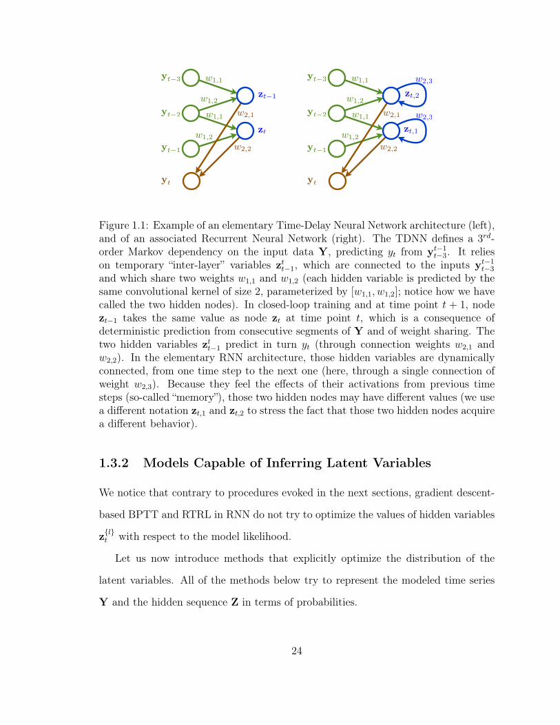
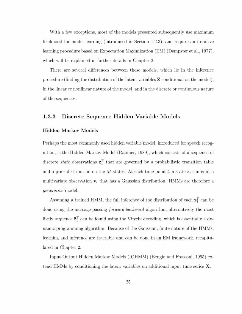
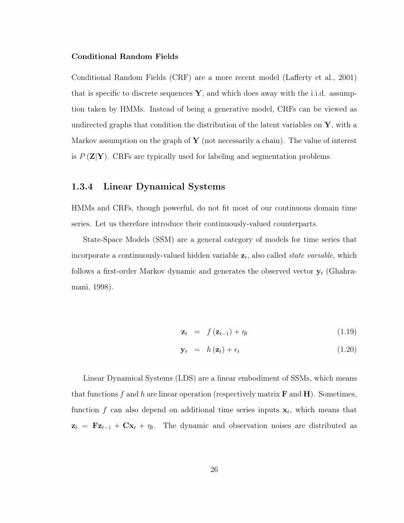
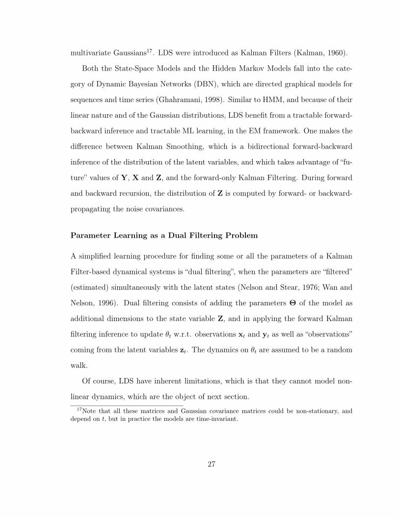
between hidden states. Figure 1.1 illustrates the difference between a TDNN and a

RNN on two toy architectures.

Unfortunately, RNNs require special learning procedures, and ML algorithms

based on exact gradient descent (Rumelhart et al., 1986) such as Backpropagation

Through Time (BPTT) or Real-Time Recurrent Learning (RTRL) (Williams and

Zipser, 1995), fail. The well-known problem of vanishing gradients is responsible for

RNN to forget, during training, outputs or activations that are more than a dozen

time steps back in time (Bengio et al., 1994). Several alternative training algorithms

have been proposed to avoid the vanishing gradient problem in RNN. One of them

consists in using Kalman Filtering as a second-order method to optimize the weights

of the RNN (Puskorius and Feldkamp, 1994). Another one, called Long Short-Term

Memory (LSTM) consists in designing a new type of units with gates that prevent

these nodes from forgetting information (Hochreiter and Schmidhuber, 1995; Wierstra

et al., 2005).

23

yt−2

yt−1

yt

w1,1

w1,2

w1,1

w1,2

w2,2

w2,1

w2,3

w2,3

yt−3

yt−2

yt−1

yt

zt−1

zt

w1,1

w1,2

w1,1

w1,2

w2,2

w2,1

yt−3

zt,1

zt,2

Figure 1.1: Example of an elementary Time-Delay Neural Network architecture (left),and of an associated Recurrent Neural Network (right). The TDNN defines a 3rd-order Markov dependency on the input data Y, predicting yt from yt−1

t−3. It relieson temporary “inter-layer” variables ztt−1, which are connected to the inputs yt−1

t−3

and which share two weights w1,1 and w1,2 (each hidden variable is predicted by thesame convolutional kernel of size 2, parameterized by [w1,1, w1,2]; notice how we havecalled the two hidden nodes). In closed-loop training and at time point t + 1, nodezt−1 takes the same value as node zt at time point t, which is a consequence ofdeterministic prediction from consecutive segments of Y and of weight sharing. Thetwo hidden variables ztt−1 predict in turn yt (through connection weights w2,1 andw2,2). In the elementary RNN architecture, those hidden variables are dynamicallyconnected, from one time step to the next one (here, through a single connection ofweight w2,3). Because they feel the effects of their activations from previous timesteps (so-called “memory”), those two hidden nodes may have different values (we usea different notation zt,1 and zt,2 to stress the fact that those two hidden nodes acquirea different behavior).

1.3.2 Models Capable of Inferring Latent Variables

We notice that contrary to procedures evoked in the next sections, gradient descent-

based BPTT and RTRL in RNN do not try to optimize the values of hidden variables

zlt with respect to the model likelihood.

Let us now introduce methods that explicitly optimize the distribution of the

latent variables. All of the methods below try to represent the modeled time series

Y and the hidden sequence Z in terms of probabilities.

24

With a few exceptions, most of the models presented subsequently use maximum

likelihood for model learning (introduced in Section 1.2.3), and require an iterative

learning procedure based on Expectation Maximization (EM) (Dempster et al., 1977),

which will be explained in further details in Chapter 2.

There are several differences between these models, which lie in the inference

procedure (finding the distribution of the latent variables Z conditional on the model),

in the linear or nonlinear nature of the model, and in the discrete or continuous nature

of the sequences.

1.3.3 Discrete Sequence Hidden Variable Models

Hidden Markov Models

Perhaps the most commonly used hidden variable model, introduced for speech recog-

nition, is the Hidden Markov Model (Rabiner, 1989), which consists of a sequence of

discrete state observations zT1 that are governed by a probabilistic transition table

and a prior distribution on the M states. At each time point t, a state xt can emit a

multivariate observation yt that has a Gaussian distribution. HMMs are therefore a

generative model.

Assuming a trained HMM, the full inference of the distribution of each zT1 can be

done using the message-passing forward-backward algorithm; alternatively the most

likely sequence zT1 can be found using the Viterbi decoding, which is essentially a dy-

namic programming algorithm. Because of the Gaussian, finite nature of the HMMs,

learning and inference are tractable and can be done in an EM framework, recapitu-

lated in Chapter 2.

Input-Output Hidden Markov Models (IOHMM) (Bengio and Frasconi, 1995) ex-

tend HMMs by conditioning the latent variables on additional input time series X.

25

Conditional Random Fields

Conditional Random Fields (CRF) are a more recent model (Lafferty et al., 2001)

that is specific to discrete sequences Y, and which does away with the i.i.d. assump-

tion taken by HMMs. Instead of being a generative model, CRFs can be viewed as

undirected graphs that condition the distribution of the latent variables on Y, with a

Markov assumption on the graph of Y (not necessarily a chain). The value of interest

is P (Z|Y). CRFs are typically used for labeling and segmentation problems.

1.3.4 Linear Dynamical Systems

HMMs and CRFs, though powerful, do not fit most of our continuous domain time

series. Let us therefore introduce their continuously-valued counterparts.

State-Space Models (SSM) are a general category of models for time series that

incorporate a continuously-valued hidden variable zt, also called state variable, which

follows a first-order Markov dynamic and generates the observed vector yt (Ghahra-

mani, 1998).

zt = f (zt−1) + ηt (1.19)

yt = h (zt) + εt (1.20)

Linear Dynamical Systems (LDS) are a linear embodiment of SSMs, which means

that functions f and h are linear operation (respectively matrix F and H). Sometimes,

function f can also depend on additional time series inputs xt, which means that

zt = Fzt−1 + Cxt + ηt. The dynamic and observation noises are distributed as

26

multivariate Gaussians17. LDS were introduced as Kalman Filters (Kalman, 1960).

Both the State-Space Models and the Hidden Markov Models fall into the cate-

gory of Dynamic Bayesian Networks (DBN), which are directed graphical models for

sequences and time series (Ghahramani, 1998). Similar to HMM, and because of their

linear nature and of the Gaussian distributions, LDS benefit from a tractable forward-

backward inference and tractable ML learning, in the EM framework. One makes the

difference between Kalman Smoothing, which is a bidirectional forward-backward

inference of the distribution of the latent variables, and which takes advantage of “fu-

ture” values of Y, X and Z, and the forward-only Kalman Filtering. During forward

and backward recursion, the distribution of Z is computed by forward- or backward-

propagating the noise covariances.

Parameter Learning as a Dual Filtering Problem

A simplified learning procedure for finding some or all the parameters of a Kalman

Filter-based dynamical systems is “dual filtering”, when the parameters are “filtered”

(estimated) simultaneously with the latent states (Nelson and Stear, 1976; Wan and

Nelson, 1996). Dual filtering consists of adding the parameters Θ of the model as

additional dimensions to the state variable Z, and in applying the forward Kalman

filtering inference to update θt w.r.t. observations xt and yt as well as “observations”

coming from the latent variables zt. The dynamics on θt are assumed to be a random

walk.

Of course, LDS have inherent limitations, which is that they cannot model non-

linear dynamics, which are the object of next section.17Note that all these matrices and Gaussian covariance matrices could be non-stationary, and

depend on t, but in practice the models are time-invariant.

27

Conditional State Space Models

Similar to CRF, one can define linear SSM in terms of undirected graphs, and con-

dition the continuously-valued latent variable Z on the observed variables Y, instead

of a generative model from Z to Y. This approach, with linear first-order Markov

dynamics on Z, was adopted by (Kim and Pavlovic, 2007). Latent variable inference

was done using a Kalman filter, and ML learning was done using gradient descent on

the parameters18.

1.3.5 Nonlinear Dynamical Systems

Suppose now that we replace linear functions f and h in Equations (1.19) and (1.20)

by any nonlinear relationship.

Because the inference in DBN is probabilistic, a closed-form solution might not

exist, and that inference might become difficult or even intractable in the case of

highly nonlinear dynamics and observation models, as is illustrated with the diffi-

culties encountered by so-called Extended Kalman Filters/Smoothers. The root of

the problem is in the propagation of the covariance matrices: the nonlinearity that

predicts zt+1 from zt makes the distribution of zt+1 no longer Gaussian. Because of

the issues with latent variable inference, and because of the partition function prob-

lem explained in Section 2.2.2, the learning of the parameters is made all the more

difficult, as it cannot easily be expressed in closed form and is not tractable.

Several workarounds have been devised in the past decade, which we enumer-

ate below. Beforehand, we shall only mention that, keeping the imperfect Extended

Kalman Filter/Smoother architecture, (Wan and Nelson, 1996) devised a dual fil-18Interestingly, because the latent variables (consisting in human poses, associated to observed

silhouettes from videos) in the training dataset were known, the hidden variable model was actuallytrained discriminatively.

28

tering/smoothing approach for joint state and parameter estimation, which at least

greatly simplified the learning procedure.

Unscented and Particle Filtering for Inference

A popular algorithm for latent variable inference in nonlinear models is the Unscented

Kalman Filter/Smoother (Wan and Van Der Merwe, 2000). Instead of propagating

the mean and covariance matrix of zt through the nonlinearity, the UKF propagates

the mode and 2M “particles”, 2 particles per dimension of zt, on each side of the

peak of the distribution and in each dimension. This works very well for unimodal

distributions. For more complex distributions, one can use the Particle Filter (PF),

with a cloud of (thousands of) particles zt propagated at each time step, out of

which one can sample the distribution of zt. UKF and PF resort to joint filtering for

parameter estimation, though.

Making the Learning Tractable

The main issue with learning Nonlinear Dynamic Systems, and hidden variable models

in general, will be explicited in Section 2.2.2, and is linked to the fact that one can-

not properly compute the probability distribution over Z, because of the intractable

partition function (in short, one would need to sum over all the possible values of

Z, which can be done easily only for a limited number of distributions such as the

Gaussian). As a consequence, DBNs that are more complex than LDS and HMMs

break out once certain nonlinear architectures are designed (Ghahramani, 1998).

Several approaches have been designed to overcome the issue of the partition

function, including the expensive sampling techniques, and the sometimes compli-

cated Variational Bayes derivations to the EM learning procedure. Those approxi-

mate techniques enable approximate inference of the full distribution of the hidden

29

variables19.

On one hand, (Ghahramani and Roweis, 1999) introduced an NDS where the

dynamic function f consisted of Radial Basis Functions, i.e. a mixture of Gaussians.

This enabled an exact inference and learning steps in the EM algorithm, but required

the RBF centers to be properly initialized.

On the other hand, (Ilin et al., 2004) simplified the NDS to first-order Markov

dynamics (it was effectively an SSM), where the nonlinearities were represented by

Multi-Layer Perceptrons (MLP) with one hidden layer with tanh nonlinearity. This

enabled to devise a variational Bayes approximation for approximating the distribu-

tion of Z. Their algorithm was applied to model chaotic attractors and to detect

changes in nonlinear dynamics.

Both the RBF and MLP nonlinearities employed in NDS were relatively simple

compared to the kind of nonlinearities (convolutional networks) used in Chapter 3 of

this doctoral work.

NDS with Approximate Inference of Hidden Variables

An early model of nonlinear dynamical system with inferred hidden variables is the

Hidden Control Neural Network (Levin, 1993), where a latent variable z(t) is added

as an additional input to mapping (1.2). Although the dynamical model remains

unchanged (thus stationary) across the whole time series, the latent variable z(t)

modulates the dynamics of (1.2), enabling a behavior more complex than in pure

autoregressive systems. The training algorithm iteratively optimizes the sequence

Z of latent variables (1.21) and the weights W of the Time-Delay Neural Network19As explained in the next chapter, I used in my doctoral work a different approach to the inference

of hidden variables, performing maximum a-posteriori inference of the most likely configuration ofthe hidden variables. By “cutting corners” in the inference process, my technique is able to handle amuch richer class of nonlinearities (essentially, any kind of nonlinear function that is differentiable)than traditional graphical models.

30

(TDNN) (equation 1.22):

Z = arg minZ′

E (Y (t),W,Z′) = arg minZ′

∑

t

‖ yt − f (yt−1,Z′; W) ‖2

2 (1.21)

W = arg minW′

E (Y,Z; W′) (1.22)

The latter algorithm, which is likened to approximate maximum likelihood train-

ing, is the starting point for my own method, which relies on the same iterative

learning, but instead of finding a sequence of dynamic-modulating latent variables,

finds the latent variables Z that generate the observations Y, as in DBNs. Moreover,

I propose to consider non-Markovian (or higher-order Markovian) dynamics where

hidden states zt depend on a time-delay embedding of zt−1t−p.

A more recent model of DBN with deterministic dynamics and explicit inference

of latent variables was introduced in (Barber, 2003). However, the inference of the

hidden variables was done by message passing in the forward direction only, and

the dynamics were first-order Markov only. Both these algorithms were successfully

applied to short-sequence speech recognition problems.

1.3.6 Mixed Models for Switching Dynamics

A large area of research has been focusing on mixed state-space models that model

switching dynamics and cope with nonstationarity. For instance (Kohlmorgen et al.,

1994, 1998) employ a mixture of HMMs and Neural Networks experts (such as Radial

Basis Functions RBF) for identification of wake/sleep in physiological recordings,

whereas (Pavlovic et al., 1999) employs a mixture of HMMs and LDS for modeling

and classifying time series corresponding to different motions.

31

1.3.7 Recurrent Boltzman Machines

An alternative nonlinear generative model with explicit inference of latent variables

is the Restricted Boltzman Machine (RBM). RBMs contain stochastic binary latent

variables and real-valued observations (Hinton et al., 1995) with an EM-like inference

and learning procedure. Multilayer RBM architectures (Hinton et al., 2006) enable

non-linear dynamics, and (Sutskever and Hinton, 2006) enables pth order temporal

dependencies on the latent and visible units. Although difficult and long to train,

RBMs have been successfully applied to difficult time series, such as motion recon-

struction and even long-term prediction (Taylor et al., 2006). Their stochastic nature

enables them to create more interesting but still realistic trajectories and to “jump”

out of fixed attractors.

1.3.8 Gaussian Processes with Latent Variables

It is possible to incorporate lower-dimension latent variables into Gaussian Processes

Latent Variable Models (GPLVM). In that case, one expresses the probability of the

observed variables Y conditional on X by using a covariance matrix based on a Gaus-

sian kernel on X, and in the ML formulation, tries to maximize the log-likelihood not

only w.r.t. the hyperparameters of the kernel function, but also w.r.t. the kernel

matrix itself. Because of computational complexity involved in that learning pro-

cess, a special kernel algorithm is required (Lawrence, 2004). The GPLVM can be

extended by adding dynamics to X (Wang et al., 2006a), notably by expressing xt as

a Gaussian Process on xt−1. The Gaussian Process Dynamical Model (GPDM) thus

comprises a low-dimensional latent space with associated dynamics, and a map from

the latent space to an observation space, with a closed-form marginalization of the

model parameters for both the dynamics and the observation mappings.

32

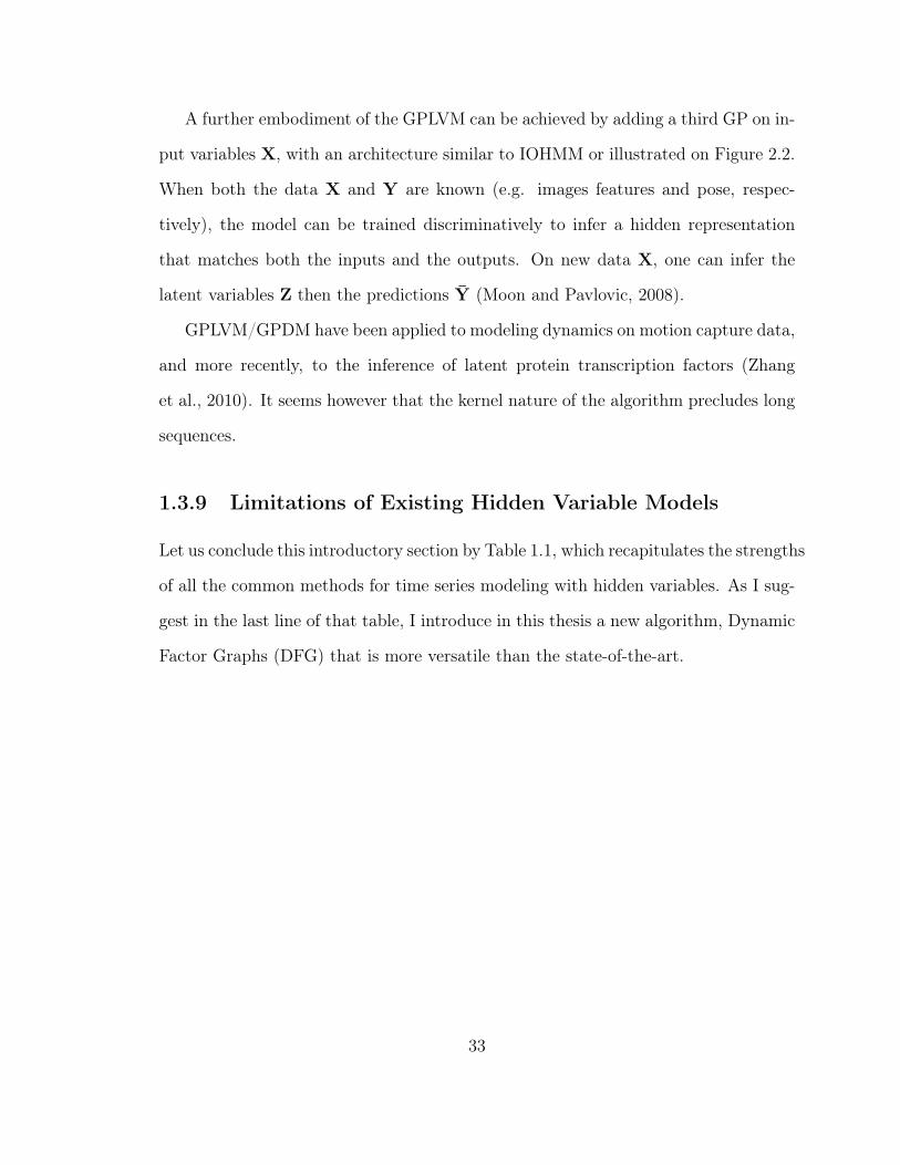
A further embodiment of the GPLVM can be achieved by adding a third GP on in-

put variables X, with an architecture similar to IOHMM or illustrated on Figure 2.2.

When both the data X and Y are known (e.g. images features and pose, respec-

tively), the model can be trained discriminatively to infer a hidden representation

that matches both the inputs and the outputs. On new data X, one can infer the

latent variables Z then the predictions Y (Moon and Pavlovic, 2008).

GPLVM/GPDM have been applied to modeling dynamics on motion capture data,

and more recently, to the inference of latent protein transcription factors (Zhang

et al., 2010). It seems however that the kernel nature of the algorithm precludes long

sequences.

1.3.9 Limitations of Existing Hidden Variable Models

Let us conclude this introductory section by Table 1.1, which recapitulates the strengths

of all the common methods for time series modeling with hidden variables. As I sug-

gest in the last line of that table, I introduce in this thesis a new algorithm, Dynamic

Factor Graphs (DFG) that is more versatile than the state-of-the-art.

33

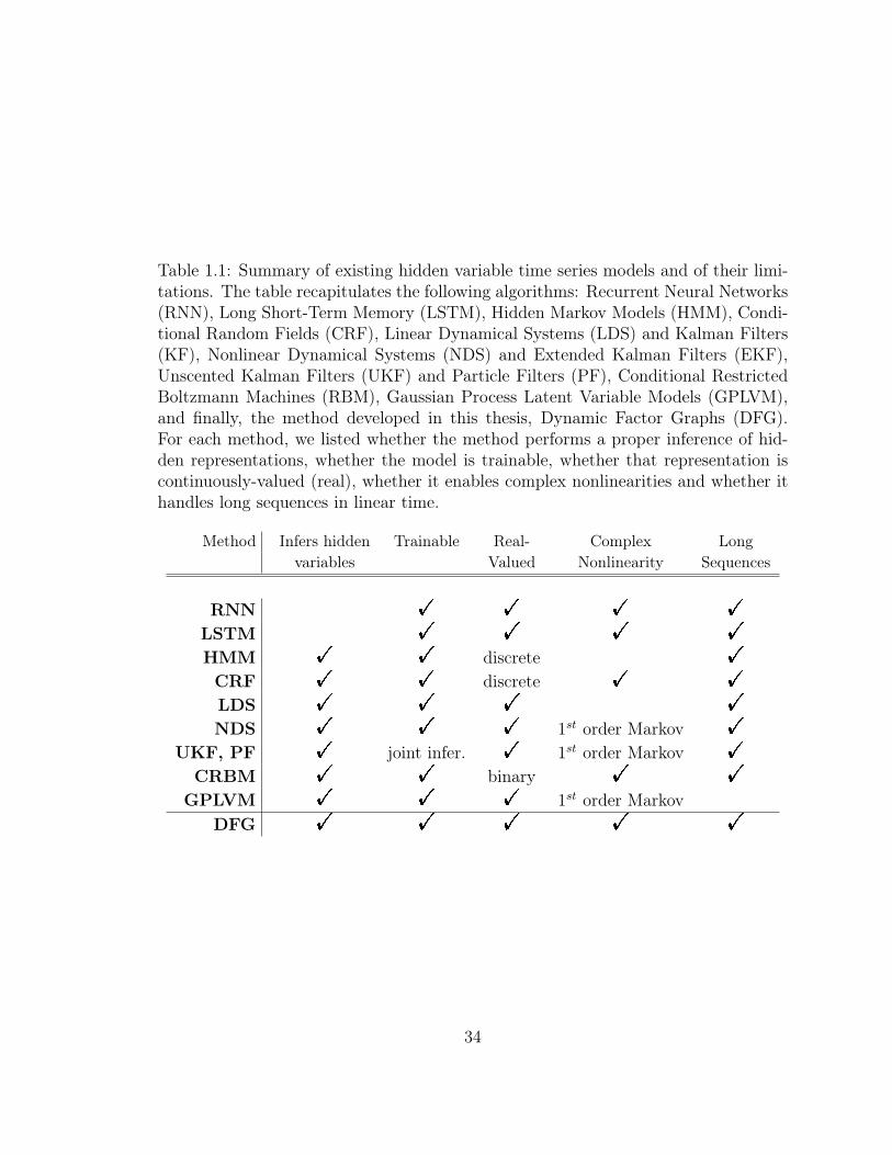
Table 1.1: Summary of existing hidden variable time series models and of their limi-tations. The table recapitulates the following algorithms: Recurrent Neural Networks(RNN), Long Short-Term Memory (LSTM), Hidden Markov Models (HMM), Condi-tional Random Fields (CRF), Linear Dynamical Systems (LDS) and Kalman Filters(KF), Nonlinear Dynamical Systems (NDS) and Extended Kalman Filters (EKF),Unscented Kalman Filters (UKF) and Particle Filters (PF), Conditional RestrictedBoltzmann Machines (RBM), Gaussian Process Latent Variable Models (GPLVM),and finally, the method developed in this thesis, Dynamic Factor Graphs (DFG).For each method, we listed whether the method performs a proper inference of hid-den representations, whether the model is trainable, whether that representation iscontinuously-valued (real), whether it enables complex nonlinearities and whether ithandles long sequences in linear time.

Method Infers hidden Trainable Real- Complex Longvariables Valued Nonlinearity Sequences

RNN ! ! ! !

LSTM ! ! ! !

HMM ! ! discrete !

CRF ! ! discrete ! !

LDS ! ! ! !

NDS ! ! ! 1st order Markov !

UKF, PF ! joint infer. ! 1st order Markov !

CRBM ! ! binary ! !

GPLVM ! ! ! 1st order MarkovDFG ! ! ! ! !

34

Chapter 2

Common Framework: Dynamical Factor Graphs

Let’s do the time warp again!

Richard O’Brien

In this chapter, I explain how we define a new inference and training algorithm

for modeling time series with Recurrent Neural Networks, using approximate iterative

inference and learning algorithms derived from state-space model such as Dynamic

Bayesian Networks, and using the Factor Graphs formalism. I will stress the impor-

tance on the most important contribution of this doctoral thesis, which is to perform

Maximum A Posteriori inference of continuously-valued hidden variables, while main-

taining the partition function constant by construction, thereby enabling to model

any kind of differentiable nonlinear dynamics and observation functions (in particu-

lar, any Markov order p), and thus achieving a much stronger representative power

than usual Graphical Models.

35

2.1 Our Factor Graph formalism

2.1.1 Factor Graphs

According to their definition (Kschischang et al., 2001; Bishop, 2006), a factor graph

is a bipartite graph with two types of nodes, variables yt and factors gi (which are

functions of variables). Each variable node can be connected only to factor nodes,

and each factor node can be connected only to variables nodes. Factor graphs express

a global function g of all variables as a product of functions on the subset of variables

to which they are directly connected. It means that function gi takes as arguments

only variables ytt∈Sito which it is directly connected in the graph. For T variables

and P functions, we have the following factorization:

g (y1,y2, . . . ,yT ) =P∏

i=1

gi(ytt∈Si

)(2.1)

Because of their factorial nature, factor graphs can represent, among others,

bayesian models (such as Hidden Markov Models), modeling the joint probability

of the full model as a product of conditional probabilities at each factor. Even if

ones does not use probabilities but hard constraints (one constraint per factor), the

conjunction of all the hard constraints in the model can be expressed as a product of

boolean indicators, one per factor (Kschischang et al., 2001).

When the graph structure is a tree, one can directly compute the marginal function

g (yt) for any variable yt using the sum-product algorithm for factor graphs, which is

based on message passing between the variable nodes. The sum-product algorithm

is the factor graph equivalent of both the forward-backward algorithm for hidden

sequence inference and of the Viterbi algorithm in HMMs, and for linear dynamical

36

zt+1zt−1zt−2 zt

yt yt+1yt−1yt−2

h

f

zt+1zt−1zt−2 zt

yt yt+1yt−1yt−2

h

f

zt+1zt−1zt−2 zt

yt yt+1yt−1yt−2

h f

zt+1zt−1zt−2 zt

yt yt+1yt−1yt−2

h f

Figure 2.1: Several Dynamic Factor Graphs that admit observed variables Y andlatent variables Z, which are factorized by observation (h) and dynamic (f) factors.

systems, corresponds to Kalman filtering (Kschischang et al., 2001). Figure 2.1 (top

left) illustrates the factor graph representation that is common to HMM and to one

embodiment of the algorithms discussed in the next chapters (specifically, the one we

used for learning the gene regulation network of the Arabidopsis in Chapter 4).

Several state-space models consist in Directed Acyclic Graphs (DAG), but an

undirected factor graph representation cannot be represented by a tree. The sum-

product algorithm nevertheless works for undirected factor graphs with cycles, it

simply needs to be repeated and has no guarantees of convergence (in the general

case). Figure 2.1 illustrates other factor graphs architectures that I will use. Among

others I investigated n-th order Markov dependencies (top right of the figure) for

modeling chaotic dynamics in Chapter 3. For the inference of protein transcription

factors in Chapter 4, I used observation and dynamic models that expressed the rates

of change of yt and of zt (bottom part of the figure). Finally, Figure 2.2 shows

37

xt xt+1xt−1xt−2

zt+1zt−1zt−2 zt

yt yt+1yt−1yt−2

fg

h

Figure 2.2: Dynamic Factor Graph that admits two types of observed variables:inputs X and outputs Y, as well as latent variables Z, which are all factorized byobservation (h), dynamic (f) and input (g) factors.

an input-output architecture that separates observed sequences into X and Y; this

architecture corresponds to supervised auto-encoders with dynamical dependencies

between hidden variables in Chapter 5. Since all the aforementioned factor graphs

are specialized for sequence modeling, I call them Dynamic Factor Graphs.

The Factor Graph formalism has already been applied to model data where the la-

tent variable had a spatial structure, notably for modeling house prices. In that case,

the price yi of the i-th house in the dataset was considered as depending both on asso-

ciated input variables xi and on a latent desirability factor zi that was geographically

smooth (Chopra et al., 2007).

2.1.2 Maximum Likelihood and Factor Graphs

As I suggested in the first chapter, model learning and the inference of hidden repre-

sentations in this thesis is done using a maximum likelihood framework1. For numer-

ical reasons, this is performed in logarithmic space, using the negative log-likelihood1We cannot apply discriminative learning of the hidden representations because we cannot eval-

uate the partition function of our nonlinear model with continuous hidden variables.

38

instead. For the case of a Dynamical Bayesian Network such as an Input-Output

HMM (Bengio and Frasconi, 1995) (which can be described by the factor graph of

Figure 2.2), the joint likelihood (Eq. 2.2) and negative log-likelihood (Eq. 2.4) are

expressed as:

P (X,Y,Z) =∏

t

P (zt|zt−1)P (zt|xt)P (yt|zt)P (xt) (2.2)

NLL = − logP (X,Y,Z) (2.3)

NLL = const+∑

t

− logP (zt|zt−1)− logP (zt|xt)− logP (yt|zt)(2.4)

Consistently with DBNs, we keep the factor graph formalism while operating in

the logarithmic space, which simply means that we add each factor’s contributions

instead of multiplying them.

2.1.3 Factors Used in This Work

Different factors will be detailed in subsequent chapters, but we can express now

their common properties. Our factors contain two modules. The first one consists

in a deterministic function (let us call it g) that takes argument variables at and

generates prediction variables ot. Those predictions are then compared to the actual

target variable ot and an error term is computed. The function that evaluates the

error constitutes the second module of the factor. Function g is parameterized by

parameters W, which we shall learn in order to minimize the prediction error of the

factor. Figure 2.3 recapitulates these concepts.

We notice that factor graphs are undirected; one can see them as “springs” between

variables. The main idea in our algorithm is that even if the functions are directed

39

(from arguments to predictions), the error term is not. Therefore, during inference

of latent variables, one can try to minimize the error by acting both on the latent

variable arguments of the function and on the latent variable that are targets of that

same function. This principle is similar to Kalman smoothing, which is bidirectional,

as opposed to Kalman filtering (Kalman, 1960), which is forward only.

at

g (at;W)

ot

ot

E (at,ot)

error (ot, ot)

Figure 2.3: General description of a factor linking variables at and ot through functiong, with energy term E (at,ot).

We considered several types of functions g in this work, enumerated below:

• identity function, for instance for modeling random walk dynamics on latent

variables, or latent variables that are a de-noised version of observed variables:

ot = at

• linear matrix operations: ot = Wat,

• linear matrix operations followed by a nonlinearity such as the hyperbolic tan-

gent tanh: ot = tanh (Wat),

• linear matrix operations followed by a softmax function, to produce probability

distributions over the output dimension space: ∀k, ok,t = ewkatPj e

wjat ,

40

• a highly nonlinear TDNN or convolutional network, typically for modeling

chaotic dynamics on the latent variables. Note that contrary to (LeCun et al.,

1998a), we did not resort to 2D convolutions, as we used only convolutions

across time, not across channels.

Similarly, we considered different types of errors, which would all correspond to

negative log-likelihoods: most commonly the sum of squares (Gaussian distribution)

and sum of absolute values (Laplace), but also the logistic error (Binomial) and

the cross-entropy error (Multinomial) for classification. The latter two errors are

reminded in Chapters 5.

2.2 Maximum Likelihood Energy-Based Inference

Now that we have defined the building blocks of our architecture, involving latent and

hidden variables, we would like to be able to infer the sequence of hidden variables

Z that optimally represents the observed sequence Y (and X, if relevant) under the

model. This is a simpler problem than that of inferring a full distribution over Z,

which is normally done for Dynamic Bayesian Networks and (Non)-Linear Dynamical

Systems (Ghahramani, 1998; Ghahramani and Roweis, 1999).

2.2.1 Energy as Negative Log-Likelihood

Let us introduce the notion of energy, which is among others reviewed in (LeCun

et al., 2006). Using the notation from Figure 2.3, our energy term E (at,ot) at each

factor merely corresponds to the error that results from predicting ot instead of ot.

Using the factor graph formalism in the logarithmic domain, the energy of the whole

sequence of observed and hidden variables is a sum of energies at all the factors,

41

and is noted E (Y,Z) or E (X,Y,Z). Without loss of generality, let us focus on

models without inputs X, and also include the model parameters W into the energy

term: E (Y,Z; W). As we mentioned earlier, we make our energy proportional to

the negative log-likelihood of joint variables Y and Z:

E (Y,Z; W) ∝ − logP (Y,Z|W) + const (2.5)

2.2.2 Intractable Partition Functions

Note that energy in Equation (2.5) does not define by itself a probability distribu-

tion, because the normalization terms are unknown. For a proper normalization and

to obtain the actual value of P (Y,Z|W), one would need to resort to the so-called

Boltzmann distribution (LeCun et al., 2006) with an additional “temperature” co-

efficient 1/β (Eq. 2.6). The Boltzmann distribution, used in statistical mechanics,

provides with the maximum entropy distribution2 that is still compatible with the

observations.

P (Y,Z|W) =e−βE(Y,Z;W)

∫Y′

∫Z′ e−βE(Y′,Z′;W)dY′dZ′

(2.6)

=e−βE(Y,Z;W)

ΓY,Z(2.7)

The normalization constant ΓY,Z is called the partition function.

For a given configuration of energies E(Y,Z|W), the lower the temperature 1/β,

the more peaked the associated Boltzmann distribution (conversely, the higher the

temperature, the more uniform the distribution). At sufficiently low temperatures, in2i.e. most uniformly random

42

the limit of β →∞, the associated distribution would become unimodal, even if the

energy surface admitted local minima; therefore, the joint configuration of observed

and hidden variables given the model would seem simpler than it actually is.

In order to evaluate the likelihood of observed sequence Y, one needs to marginal-

ize P (Y,Z|W) and (Eq. 2.6) over all the values that hidden sequence Z can take:

P (Y|W) =

∫

Z′P (Y,Z′|W) dZ′ (2.8)

=

∫

Z′

e−βE(Y,Z′;W)

∫Y′

∫Z′′ e−βE(Y′,Z′′;W)dY′dZ′′

dZ′ (2.9)

Evaluating the integrals of (Eq. 2.6) and (Eq. 2.9) over all observed and hidden

sequences is intractable for continuous variables under non-Gaussian distributions. It

is similarly difficult when the distributions are Gaussian but the factors are nonlinear.

As we detailed in the first chapter, DBN, LDS and NDS algorithms have resorted to

various approximations involving sampling and variational Bayes approximations.

2.2.3 Maximum A Posteriori Approximation

Similarly to previous work in that field conducted in Prof. LeCun’s lab (LeCun et al.,

2006; Chopra et al., 2007; Ranzato et al., 2007), we propose to use a maximum a

posteriori (MAP) approximation, which foregoes the full distribution in favor of its

mode. What follows is an analogy to the proofs derived in (Ranzato, 2009).

Let us first define the “marginal” energy of the observed sequence Y, after having

integrated away the latent variables. This definition is arbitrary but fits nicely into

previous equation (2.9):

43

E (Y; W) = − 1

βlog

∫

Z′e−βE(Y,Z′;W)dZ′ (2.10)

e−βE(Y;W) =

∫

Z′e−βE(Y,Z′;W)dZ′ (2.11)

P (Y|W) =e−βE(Y;W)

∫Y′ e−βE(Y′;W)dY′

(2.12)

We will show that a) E (Y; W) can be approximated by arg minZE (Y,Z; W),

and that b) arg minZE (Y,Z; W) = arg maxZ P (Z|Y,W). Let us begin with the

second statement.

By the Bayes rule P (Y,Z|W) = P (Z|Y,W)P (Y|W), maximizing P (Y,Z|W)

w.r.t. Z is akin to maximizing P (Z|Y,W) w.r.t. Z since P (Y|W) does not depend

on Z. Then, using Equation (2.6), arg maxZ P (Z|Y,W) = arg maxZ e−βE(Y,Z;W)

because the partition function is independent of the variables. Hence:

arg minZE (Y,Z; W) = arg max

ZP (Z|Y,W) (2.13)

Now, to prove that E (Y; W) can be approximated by arg minZE (Y,Z; W), we

take Equation (2.10) to the limit in β. Assuming that the energy E (Y,Z; W) is

positive and admits a zero minimum in Z0 (which is the case for instance for quadratic

errors):

limβ→∞

− 1

βlog

∫

Z′e−βE(Y,Z′;W)dZ′ = lim

β→∞− 1

βlog

∫

Z′δZ′=Z0e

−βE(Y,Z′;W)dZ′(2.14)

= limβ→∞

− 1

βlog(e−βE(Y,Z0;W)

)(2.15)

= E (Y,Z0; W) (2.16)

44

In the rest of this work, we subsequently note that, for an observed sequence Y

and given a model parameterized by W, the result of the latent variable inference is

the minimum energy state of the model for that sequence:

E (Y; W) = arg minZE (Y,Z; W) (2.17)

2.2.4 Summing Energies from Diverse Factors

As illustrated on Figures 2.1 and 2.2, our factor graphs contain several types of factors

replicated over the time dimension of the sequences. We therefore need to sum up,

for all time points, energies from various factors.

We design our factor graph and energy functions under the assumption that all

time series including the latent variables Z are identically distributed, with conditional

independencies beyond the reach of each factor (see section 1.2.3). This means that

for a given type of factor, the additive normalization term (due to the partition

function) − log ΓZ,Y (t) remains constant across time samples t ∈ 1, . . . , T. This

also means that, for exponential distributions (such as Laplace and Gaussian), the

multiplicative scale coefficients for each data point are constant across time. Recall

that for the Gaussian distribution, these scale coefficients are linked to the inverse of

the covariance matrix Σ. As many latent variable techniques in the machine learning

literature do, we will claim3 that the covariance matrix is diagonal with identical

terms across the diagonal: Σ = σI.

However, because we did not properly normalize the energies of our factors, we

are left with “guessing” the relative weight of the scales σ for each type of factors. For

a clearer picture, let us focus for instance on a DFG composed of observation h and3We can of course design latent variables such that their covariance is diagonal, and we can

always standardize the observed time series Y to zero-mean and unit variance for each dimension,and then apply a principal component analysis to de-correlate the rows of Y.

45

dynamic f factors (as in Chapters 3 and 4), with associated energies Eh (yt, zt; W)

and Ef(zt−1t−p, zt; W

). Let us assume (as is the case in those chapters) that their

underlying distributions are Gaussian, which also means that their error terms are

Gaussian:

∀t, P (yt − h (zt; W) |zt) ∼ N (0,Σh) = N (0, σhIN) (2.18)

∀t, P(zt − f

(zt−1t−p; W

))∼ N (0,Σf ) = N (0, σfIM) (2.19)

In our energy-based framework, we simply replace the scales σh and σf by their

relative weight coefficient γ (e.g. coefficient of the dynamic factor). The total energy

of a sequence of observed Y and hidden variables Z is written as (Eq. 2.20), and the

inference problem becomes (Eq. 2.21).

E (Y,Z; W) =∑

t

Eh (yt, zt; W) + γ∑

t

Ef(zt−1t−p, zt; W

)(2.20)

E (Y; W) = arg minZ′

∑

t

Eh (yt, zt; W) + γ∑

t

Ef(zt−1t−p, zt; W

)

(2.21)

We can use a few tricks to make the guessing of γ easier. First of all, if there are

several factors with similar types of energies (e.g. Gaussian sum of square errors), then

we can normalize the energies by the number of dimensions of the variables involved.

Secondly, varying the relative contributions of each factor type can be treated like

adjusting additional hyper-parameters with an intuitive explanation: the coefficient

γ is related to the “weight” or “importance” we want to give to the dynamic factor;

the larger the γ, the tighter the scale or bandwidth of that factor. Finally, γ can be

46

adjusted with the usual arsenal of techniques such as cross-validation.

2.2.5 Interpretation in Terms of Lagrange Multipliers

Another explanation of the γ can be provided from the Lagrange multipliers tech-

nique, developed by French mathematician Joseph Louis Lagrange. Let us consider

indeed the energy minimization problem (Eq. 2.17) with two factors4, one for the

observation (h) and one for the dynamics (f), as a constrained optimization problem

with an objective (Eq. 2.22) and a constraint (Eq. 2.23):

minZEh (Y,Z; W) (2.22)

subject to: ∀t, zt = f (zt−1; W) (2.23)

The Lagrange multiplier technique proposes to integrate those constraints into one

Lagrange function Λ (Z, λ), after multiplying each constraint (over all time points and

for all M dimensions of Z) by a corresponding Lagrange coefficient λk,t:

Λ (Z, λ) = Eh (Y,Z; W) +T∑

t=2

M∑

k=1

λk,t (zk,t − fk (zt−1; W)) (2.24)

The Lagrange function enables to define the notion of a Lagrangien Λ (λ), which is

a lower bound on Λ for a specific configuration of the Lagrange multipliers (Eq. 2.25).

We can set equal constraints on all time points (conditional i.i.d. assumption) and

on all dimensions of Z (not favoring one hidden dimension over another), to obtain a

simplified Lagrangien depending on a single variable (Eq. 2.26).4For simplicity, but without loss of generality, we assumed that the Markov order p was one in

constrain (Eq. 2.23).

47

Λ (λ) = minZ

Eh (Y,Z; W) +

T∑

t=2

M∑

k=1

λk,t (zk,t − fk (zt−1; W))

(2.25)

= minZ

Eh (Y,Z; W) + λ

(T∑

t=2

M∑

k=1

(zk,t − fk (zt−1; W))

)(2.26)

The last equation (Eq. 2.26) shows the analogy to the energy-based inference (Eq.

2.21). Note however that in numerical optimization, the solution (Z, λ) to the La-

grange optimization does not correspond to the optimum of Λ (Z, λ), but rather to a

so-called saddle-point or critical point, which is at the same time a minimum w.r.t.

Z and a maximum w.r.t. the Lagrange coefficients λ.

2.2.6 Inference of Latent Variables

As we will illustrate in the next chapters, inference of latent variables in an MAP

setting becomes extremely simple. For a given configuration of the pseudo-Lagrange

coefficients, one simply needs to find the optimum of E (Y,Z; W), i.e. to differentiate

the total sequence energy (Eq. 2.20) w.r.t. the latent variables, and therefore to solve

for:

∂E (Y,Z; W)

∂Z= 0 (2.27)

This can be achieved using the well-known gradient descent algorithm. As evoked

earlier, we back-propagate (Rumelhart et al., 1986) the gradients from the energy

modules in both directions, and update each zt by summing up the contributions

coming from all the factors it is connected to. We repeat the gradient step using a

48

small learning rate, until a convergence criterion.

2.2.7 What DFGs Can Do That Graphical Models Cannot

The most important contribution of this doctoral thesis can be summarized in a single

sentence: Thanks to our Maximum A Posteriori approximation during the inference of

continuously-valued hidden representations of time series, and because we maintain

the partition function constant by construction, we are able to model any kind of

differentiable nonlinear dynamics and observation functions, with any dependencies

between the variables (in particular, any Markov order p), achieving a much stronger

representative power than usual Graphical Models.

2.2.8 On the Difference Between Hidden and Latent Variables

I would like to highlight at this point the difference between hidden and latent vari-

ables Z. Both are variables that are not observed and that need to be extracted from

observed data. However only the latent variables correspond to a maximum likelihood

solution that is obtained through inference. The maximum likelihood solution corre-

sponds to the mode of the distribution of Z for DBNs, and to the minimum energy

sequence w.r.t. Z for our DFGs. If we think in terms of message passing through the

factor graph, a hidden representation is obtained through a simple “forward” mes-

sage passing (e.g. direct prediction by an encoder), whereas the latent representation

is obtained after an iteration of “forward” and “backward” message passings, in a

so-called relaxation procedure, until the hidden representation converges to a stable

fixed point.

As such, the hidden variables in the language modeling task from Chapter 6 are

not properly latent, since they are obtained through a deterministic look-up table

49

from a discrete observed sequence yT1 , without a relaxation step w.r.t. the dynamic

energy linking the hidden variables. We abstained from full relaxation on the hidden

variables because of the computational complexity of the language model on large

vocabularies and large text corpora.

2.3 Expectation Maximization-Like Learning of DFG

2.3.1 Expectation Maximization Algorithm

In its original form, Expectation Maximization (EM) (Dempster et al., 1977) is an

iterative and probabilistic maximum likelihood algorithm for estimating missing data

and learning the parameters of the joint distribution of observed and missing data.

EM alternates between parameter estimation/learning (M-step) and latent variables

inference (E-step), and can be referred to as coordinate ascent of the likelihood. The

main limitation of EM is that it converges to a local maximum likelihood.

In a nutshell, EM strives at maximizing the joint likelihood P (Y,Z|Θ) of com-

plete data (observed and hidden) that one could obtain given a model parameterized

by Θ. In other words, it tries to find the optimal Θ such that P (Y,Z|Θ) is max-

imal. Because Z is unknown, it tries instead to maximize the expectation of the

log-likelihood of the complete data under the model. The first step (E-step) consists

in evaluating E[logP

(Y,Z|Θ(k)

)]given the current estimate Θ(k)of the parameters.

The second step (M-step) consists in maximizing that quantity with respect to the

parameters Θ, i.e. assigning Θ(k+1) = arg maxΘ E[logP

(Y,Z|Θ(k)

)].

As one can guess, the quantities enunciated above can be evaluated in closed

form if one can compute the full distribution P (Y,Z|Θ), for instance in HMM or

LDS. It is however more difficult in the case of intractable partition functions and

50

distributions. An alternative explanation of EM, in terms of free energy and entropy

is given in (Ghahramani, 1998). In particular, the distribution P (Y,Z|Θ), which

is unknown, is replaced by an approximate distribution Q (Y,Z|Θ) that is known,

and during the E-step, instead of maximizing the expectation of P (Y,Z|Θ), one

maximizes the log-likelihood of Q (Y,Z|Θ), which is proved to be a lower bound on

the log-likelihood of P (Y,Z|Θ)5.

Since its inception, EM has found a wealth of applications in many fields, for

instance in various fields of signal processing (Moon, 1996). Generalized EM (GEM)

is a version of EM with truncated M-step that only partially improves the likelihood

of the parameters given the latent variables inferred in the E-step. Stochastic and

incremental (Neal and Hinton, 1998) variants of the EM are also possible.

2.3.2 Our Simplification and Approximation

The link between EM and our work is very simple, albeit simplistic. As we said

earlier, instead of evaluating the full distribution P (Y,Z|Θ) (or P (Z|Y,Θ), for that

matter) we replace it by its MAP approximation (its argmax). Then, maximizing the

conditional likelihood of the hidden variables is equivalent to minimizing the energy,

according to Equation (2.13). Since we are treating the “inferred” distribution of Z as

its mode, or more plainly, as a fixed quantity (just like Y), we can solve the M-step

learning in a quantity of ways.

2.3.3 Alternated E-Step and M-Step Procedure

In summary, learning in an DFG consists in adjusting the parameters W in order to

minimize the sum of energies at each factor. Because we introduce a regularization5Such a formulation is useful for Variational Bayes inferrence (MacKay, 2003).

51

term R (W) on the parameters (see Section 1.2.10) as well as another regularization

term Rz(Z) on the latent representation (see Section 2.4.2), we speak instead of a

loss function L(Y,Z; W), defined in Equation (2.28). That loss function contains a

crucial additional term, the log partition function − log ΓY,Z , which is constant by

construction in our case and can by consequence be ignored during minimization.

Coming back to the example exhibited in the last section, the iterative procedure can

be written as:

L(Y,Z; W) =∑

t

(Eh(t) + γEf (t)) +Rz(Z) +R (W)− log ΓY,Z (2.28)

E-step: Z = arg minZ′

L(Y,Z′; W) (2.29)

M-step: W = arg minW′

L(Y,Z; W′) (2.30)

Minimization of the loss is done iteratively in an Expectation-Maximization-like

fashion in which the states Z play the role of auxiliary variables. The inference

described in part and equation (2.29) can be considered as the E-step (state update)

of a deterministic gradient-based version of the EM algorithm. During the parameter-

adjustingM-step (weight update) described by (2.30), the latent variables are frozen.

This means that we are back into the non-hidden variable framework, and that we

perform any kind of optimization6 to adjust W.

The E-step inference can be done either on the full sequence, or on mini-batches

(we used sequence length ranging from 20 to 1000 samples) with an M-step parameter

update after each mini-batch inference. In the latter case, during one epoch of train-

ing, the batches should be selected randomly, similar to regular stochastic gradient6In the next chapters, we show that we investigated several ways to perform the M-step parameter

learning.

52

with no latent variables (LeCun et al., 1998b; Bottou, 2004), in order to speed up the

learning of the weight parameters.

2.4 Discussion

Hidden/latent models are not without certain limitations, which need to be handled.

This section recapitulates the three most important ones.

2.4.1 Avoiding Flat Energy Surfaces During Inference

Hidden representations may raise the issue of flat energy surfaces. This means, that

no matter what observed sequence Y is supplied to the hidden-variable model, the

model can infer a good representation Z of Y, where “good” means that its energy

E(Y) is very low (e.g. E(Y) = 0). If the model can infer the same E(Y) = 0 no

matter what Y, then it is not able to discriminate between sequences, and is not very

informative. This could typically be acute in over-complete representations, where

the dimension of the latent variables is greater than the dimension of the observed

variables (Olshausen and Field, 1997; Ranzato et al., 2007).

In his thesis on that subject (Ranzato, 2009), Marc’Aurelio Ranzato provided two

theorems and proofs that flat energy surfaces can be avoided, under some conditions.

The first condition is that the dimension M of latent variables is smaller than the

dimenion N of observed variables: this is the case for instance for all the models in

Chapter 5 and some models in Chapter 4. The second condition, when M ≥ N , is to

have a sparse prior on the latent representation Z, which corresponds to limiting the

information content of the representation.

In Chapter 3, we introduce latent variables with M > N , while in Chapter 4,

we have some models with M = N . Let us now prove, in a simple way, that our

53

dynamical constraint/model still prevents flat energy surfaces.

Without loss of generality, let us assume that the observation model h and the

dynamical model f are linear (matrices H ∈ RN×M and F ∈ RN×N), that we have the

HMM-like DFG architecture from Figure 2.1 (top-left), and that the Markov order is

p = 1, with a time series Y ∈ RN×T of length T . Then, for each time-point and for

each dimension of Y, we have a linear combination of hidden variables Z:

∀t ∈ 1, . . . , T, ∀k ∈ 1, . . . , N, yk(t) =M∑

i=1

hk,izi(t) (2.31)

This yields N × T equations of M × T unknowns (elements of Z), and we have

N × T ≤ M × T . However, the dynamical equations bring additional M × (T − 1)

equations, keeping the same M × T unknowns:

∀t ∈ 2, . . . , T, ∀i ∈ 1, . . . ,M, zi(t) =M∑

j=1

fi,jzj(t− 1) (2.32)

Trivially, provided that N × T ≤ M , the system is overdetermined. Hence we

might not find, for any Y, a solution Z that fits Y perfectly. Moreover, our en-

ergies (typically Gaussian) are not flat, but convex. Therefore, for sufficiently long

sequences, flat energy surfaces can be avoided.

The specific case of sequence likelihood estimation in Chapter 6 does not fall into

the flat energy trap, because the observation factor is a look-up table (which means

that the latent representation of a discrete sequence Y is produced deterministically),

and because the dynamical energy on sequences of hidden vectors Z integrates the

partition function, which means that for each input zt−1t−p to the dynamical function

f , there is only one possible output zt that achieves minimal energy, and that output

might be in contradiction with the embedding of yt. Hence the energy surface of all

possible sequences Y is certainly not flat: actually, we use that model to discriminate

54

between more or less “valid” sequences Y.

2.4.2 Bounding the Hidden Representation

Although the learning and inference algorithms for DFGs turn out to be simple and

flexible, and the energy surface of E (Y; W) cannot be flat, the hidden state inference

might however still be under-constrained, particularly so when the number M of

dimensions in latent variables Z is higher than the number N of dimensions of the

observed variables Y.

On one hand, there is for instance a risk that latent variables take extremely

large or extremely low values, which we would like to avoid. On the other hand, we

might want the latent variables to have a reproducible “appearance” from one learning

procedure to another, or we would like to inject a prior on that appearance.

For this reason, we propose to (in)directly constrain and regularize the hidden

variables in several ways.

Constraining the Observation Model

We could set some or all the parameters of the observation model to a fixed value. For

instance, when the latent variable represents a hidden phenomenon (e.g. a protein

transcription factor) and we want to know the influence of that phenomenon Z on

the observed time series Y, we could set the interaction between Z and one observed

variable yk to a certain value, and measure the interactions between Z and the other

observed variables yj relatively to yk (see Chapter 4).

Alternatively, when there are more hidden variables than observed variables (M >

N), we could even fix the observation model, and keep degrees of freedom of the sys-

tem only on the dynamics (see Chapter 3). Models that contain more hidden variables

55

than observed variables can indeed be useful for modeling nonlinear dynamics.

Finally, even if the observation model retains most degrees of freedom, it can be

constrained to have a fixed norm (e.g. a vector norm equal to 1). For instance if the

observation model h is a linear matrix operation, we have yt = Whzt, and because

the norm of the observed variables yt is fixed, the norm of zt is fixed as well. This

solution is typically used in sparse coding (Olshausen and Field, 1997).

Regularization of the Hidden Variables

The obvious way to bound the magnitude of latent variables is to add a regularization

penalty to the inference gradient descent (E-step). An L2-norm regularization limits

their overall magnitude, while an L1-norm enforces their sparsity both in time and

across dimensions (Tibshirani, 1996).

In the case when the hidden variables are not latent but produced directly from a

look-up table, without inference, the regularization shall be applied during parameter

learning.

A third type of constraints on the latent variables is the smoothness penalty. This

penalty is somewhat contradictory with the dynamical model f , since it forces two

consecutive variables zt and zt+1 to be similar. We can however view this penalty as an

attempt at inferring slowly varying hidden states and at reducing noisy oscillations in

the latent variables (which is particularly relevant when observations Y are sampled

at a high frequency)7. By consequence, the dynamics of the latent states become

smoother and perhaps simpler to learn:

Rz

(zt+1t

)= ||zt − zt+1||22 =

M∑

i=1

(zi(t)− zi(t+ 1))2 (2.33)

7Note that we are not merely modeling Brownian motion dynamics, because this regularizationpenalty on the hidden variables comes in addition to the other dynamics modeled by function f .

56

2.4.3 Avoiding Local Minima When Learning the Model

The author wishes he could write an extensive section on the matter of local minima

avoidance. Unfortunately, Expectation Maximization (Dempster et al., 1977) and all

derived algorithms and approximations (Neal and Hinton, 1998; Baldi and Rosen-

Zvi, 2005; Chopra et al., 2007; Ranzato et al., 2007) are prone to local minima,

which means here that depending on the initial guess of latent variables’ values or

distributions, one can end up with suboptimal solutions for the model.

Solution 1: Stochastic Learning

There are luckily a few workarounds to this problem. One of them is the inclusion

of randomness into the learning procedure, by performing alternated E-steps and M-

steps on short subsequences of the total sequence, and by selecting those subsequences

in a random order, according to the stochastic learning principle (Bottou, 2004). This

technique is used in Chapters 3 and 6.

Solution 2: Initializing Low-Dimensional Z Optimally w.r.t. Observations

Another workaround, specialized to models with a linear observation factor and where

the latent variables have fewer dimensions than the observed variables, is to initialize

the latent variables with a standard dimensionality reduction technique, such as Sin-

gular Value Decomposition, followed by Independent Component Analysis, consisting

in rotating the latent variables’ space in order to make them as independent as possi-

ble. This way, we start the optimization process with a latent variable configuration

that is already very good w.r.t. the linear observation factor, and the learning is

dedicated mostly to incorporate the dynamical factor’s (and other potential factors’)

constraints into the latent representation. This technique was utilized in Chapters 4

57

and 5.

Solution 3: Bootstrapping

Finally, when the time series to be modeled is desperately short (such as mRNA level

micro-arrays for gene regulation experiments, in Chapter 4), one can repeat the full

learning procedure multiple times, and in a bootstrapping approach, draw statistics

from all the models and inferred latent sequences.

The following four chapters all consist in various embodiments of Dynamic Factor

Graphs. In particular, Chapters 3, 5 and 6 exhibit the advantage of using a sim-

ple, efficient MAP inference of hidden representations, that enables highly-nonlinear

factors.

58

Chapter 3

Application to Time Series Modeling and to

Dynamical Systems

Prediction is very difficult,

especially about the future

Niels Bohr

This chapter presents the first application of Dynamic Factor Graphs (DFG) to

the modeling of linear or chaotic time series by learning a dynamical system on the

hidden continuously-valued representation. It has been published in (Mirowski and

LeCun, 2009) and presented at the ECML 2009 conference.

In summary, our DFG includes factors modeling joint probabilities between hid-

den and observed variables, and factors modeling dynamical constraints on hidden

variables. The DFG assigns a scalar energy to each configuration of hidden and ob-

served variables. A gradient-based inference procedure finds the minimum-energy

state sequence for a given observation sequence. Because the factors are designed to

ensure a constant partition function, they can be trained by minimizing the expected

energy over training sequences with respect to the factors’ parameters. These alter-

nated inference and parameter updates can thus be seen as a deterministic EM-like

59

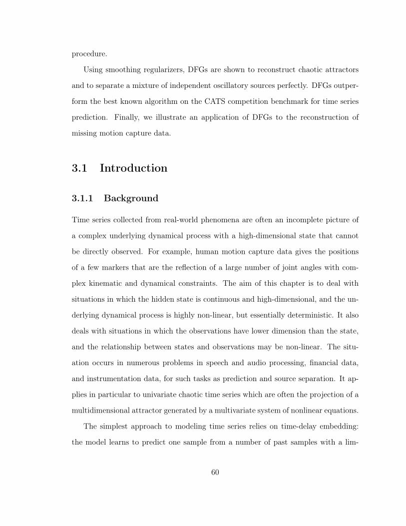
procedure.

Using smoothing regularizers, DFGs are shown to reconstruct chaotic attractors

and to separate a mixture of independent oscillatory sources perfectly. DFGs outper-

form the best known algorithm on the CATS competition benchmark for time series

prediction. Finally, we illustrate an application of DFGs to the reconstruction of

missing motion capture data.

3.1 Introduction

3.1.1 Background

Time series collected from real-world phenomena are often an incomplete picture of

a complex underlying dynamical process with a high-dimensional state that cannot

be directly observed. For example, human motion capture data gives the positions

of a few markers that are the reflection of a large number of joint angles with com-

plex kinematic and dynamical constraints. The aim of this chapter is to deal with

situations in which the hidden state is continuous and high-dimensional, and the un-

derlying dynamical process is highly non-linear, but essentially deterministic. It also

deals with situations in which the observations have lower dimension than the state,

and the relationship between states and observations may be non-linear. The situ-

ation occurs in numerous problems in speech and audio processing, financial data,

and instrumentation data, for such tasks as prediction and source separation. It ap-

plies in particular to univariate chaotic time series which are often the projection of a

multidimensional attractor generated by a multivariate system of nonlinear equations.

The simplest approach to modeling time series relies on time-delay embedding:

the model learns to predict one sample from a number of past samples with a lim-

60

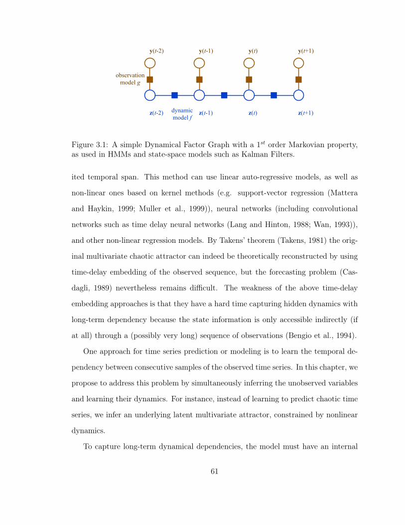
y(t-2) y(t-1) y(t) y(t+1)

z(t-2) z(t-1) z(t) z(t+1)

observationmodel g

dynamicmodel f

Figure 3.1: A simple Dynamical Factor Graph with a 1st order Markovian property,as used in HMMs and state-space models such as Kalman Filters.

ited temporal span. This method can use linear auto-regressive models, as well as

non-linear ones based on kernel methods (e.g. support-vector regression (Mattera

and Haykin, 1999; Muller et al., 1999)), neural networks (including convolutional

networks such as time delay neural networks (Lang and Hinton, 1988; Wan, 1993)),

and other non-linear regression models. By Takens’ theorem (Takens, 1981) the orig-

inal multivariate chaotic attractor can indeed be theoretically reconstructed by using

time-delay embedding of the observed sequence, but the forecasting problem (Cas-

dagli, 1989) nevertheless remains difficult. The weakness of the above time-delay

embedding approaches is that they have a hard time capturing hidden dynamics with

long-term dependency because the state information is only accessible indirectly (if

at all) through a (possibly very long) sequence of observations (Bengio et al., 1994).

One approach for time series prediction or modeling is to learn the temporal de-

pendency between consecutive samples of the observed time series. In this chapter, we

propose to address this problem by simultaneously inferring the unobserved variables

and learning their dynamics. For instance, instead of learning to predict chaotic time

series, we infer an underlying latent multivariate attractor, constrained by nonlinear

dynamics.

To capture long-term dynamical dependencies, the model must have an internal

61

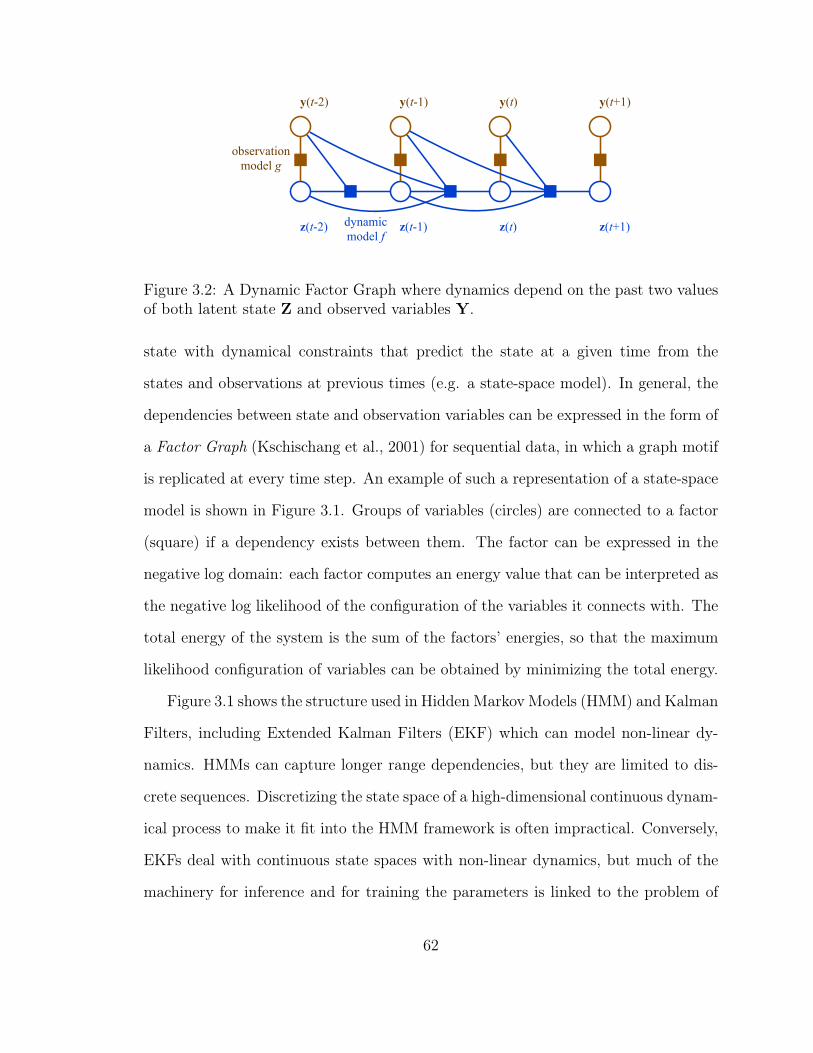
y(t-2) y(t-1) y(t) y(t+1)

z(t-2) z(t-1) z(t) z(t+1)

observationmodel g

dynamicmodel f

Figure 3.2: A Dynamic Factor Graph where dynamics depend on the past two valuesof both latent state Z and observed variables Y.

state with dynamical constraints that predict the state at a given time from the

states and observations at previous times (e.g. a state-space model). In general, the

dependencies between state and observation variables can be expressed in the form of

a Factor Graph (Kschischang et al., 2001) for sequential data, in which a graph motif

is replicated at every time step. An example of such a representation of a state-space

model is shown in Figure 3.1. Groups of variables (circles) are connected to a factor

(square) if a dependency exists between them. The factor can be expressed in the

negative log domain: each factor computes an energy value that can be interpreted as

the negative log likelihood of the configuration of the variables it connects with. The

total energy of the system is the sum of the factors’ energies, so that the maximum

likelihood configuration of variables can be obtained by minimizing the total energy.

Figure 3.1 shows the structure used in Hidden Markov Models (HMM) and Kalman

Filters, including Extended Kalman Filters (EKF) which can model non-linear dy-

namics. HMMs can capture longer range dependencies, but they are limited to dis-

crete sequences. Discretizing the state space of a high-dimensional continuous dynam-

ical process to make it fit into the HMM framework is often impractical. Conversely,

EKFs deal with continuous state spaces with non-linear dynamics, but much of the

machinery for inference and for training the parameters is linked to the problem of

62

marginalizing over hidden state distributions and to propagating and estimating the

covariances of the state distributions. This has lead several authors to limit the dis-

cussion to dynamics and observation functions that are linear, radial-basis functions

networks (Wan and Nelson, 1996; Ghahramani and Roweis, 1999) or single-hidden

layer perceptrons (Ilin et al., 2004). More recently, Gaussian Processes with dynam-

ics on latent variables have been introduced (Wang et al., 2006b), but they suffer

from a quadratic dependence on the number of training samples.

3.1.2 Dynamical Factor Graphs

By contrast with current state-space methods, our primary interest is to model pro-

cesses whose underlying dynamics are essentially deterministic, but can be highly

complex and non-linear. Hence our model will allow the use of complex functions

to predict the state and observations, and will sacrifice the probabilistic nature of

the inference. Instead, our inference process (including during learning) will produce

the most likely (minimum energy) sequence of states given the observations. We call

this method Dynamic Factor Graph (DFG), a natural extension of Factor Graphs

specifically tuned for sequential data.

To model complex dynamics, the proposed model allows the state at a given

time to depend on the states and observations over several past time steps. The

corresponding DFG is depicted in Figure 3.2. The graph structure is somewhat similar

to that of Taylor and Hinton’s Conditional Restricted Boltzmann Machine (Taylor

et al., 2006). Ideally, training a CRBM would consist in minimizing the negative

log-likelihood of the data under the model. But computing the gradient of the log

partition function with respect to the parameters is intractable, hence Taylor and

Hinton propose to use a form of the contrastive divergence procedure, which relies on

63

Monte-Carlo sampling. To avoid costly sampling procedures, we design the factors

in such a way that the partition function is constant, hence the likelihood of the

data under the model can be maximized by simply minimizing the average energy

with respect to the parameters for the optimal state sequences. To achieve this, the

factors are designed so that the conditional distributions of state z(t) given previous

states and observation, and the conditional distribution of the observation y(t) given

the state z(t) are both Gaussians with a fixed diagonal covariance matrix. Other

types of distributions (e.g. Laplace) with constant partition function are possible, all

depending on how the energy (error) is measured (e.g. sum of L1 norms for Laplace

distribution). As long as the noise term is independent of time t, we can use the

constant partition function assumption.

In a nutshell, the proposed training method is as follows. Given a training ob-

servation sequence, the optimal state sequence is found by minimizing the energy

using a gradient-based minimization method. Second, the parameters of the model

are updated using a gradient-based procedure so as to decrease the energy. These two

steps are repeated over all training sequences. The procedure can be seen as a sort

of deterministic generalized EM procedure in which the latent variable distribution is

reduced to its mode, and the model parameters are optimized with a stochastic gra-

dient method. The procedure assumes that the factors are differentiable with respect

to their input variables and their parameters. This simple procedure will allow us to

use sophisticated non-linear models for the dynamical and observation factors, such

as stacks of non-linear filter banks (temporal convolutional networks). It is important

to note that the inference procedure operates at the sequence level, and produces the

most likely state sequence that best explains the entire observation. In other words,

future observations may influence previous states.

In the DFG shown in Figure 3.1, the dynamical factors compute an energy term

64

of the form Ed(t) =‖ z(t) − f (x(t), z(t− 1)) ‖2, which can seen as modeling the

state z(t) as f(x(t), z(t− 1)) plus some Gaussian noise variable with a fixed diagonal

covariance ε(t) (inputs x(t) are not used in experiments in this chapter). Similarly,

the observation factors compute the energy Eo(t) =‖ y(t)− g(z(t)) ‖2, which can be

interpreted as y(t) = g (z(t)) + ω(t), where ω(t) is a Gaussian random variable with

fixed diagonal covariance.

Our chapter is organized in three additional sections. First, we explain the

gradient-based approximate algorithm for parameter learning and deterministic latent

state inference in the DFG model (3.2). We then evaluate DFGs on toy, benchmark

and real-world datasets (3.3). Finally, we compare DFGs to previous methods for

deterministic nonlinear dynamical systems and to training algorithms for Recurrent

Neural Networks (3.4).

3.2 Methods

The following subsections detail the deterministic nonlinear (neural networks-based)

or linear architectures of the proposed Dynamic Factor Graph (3.2.1) and define the

EM-like, gradient-based inference (3.2.2) and learning (3.2.4) algorithms, as well as

how DFGs are used for time series prediction (3.2.3).

3.2.1 A Dynamic Factor Graph

Similarly to Hidden Markov Models, our proposed Dynamic Factor Graph contains

an observation and a dynamical factors/models (see Figure 3.1), with corresponding

observed outputs and latent variables.

The observation model g links latent variable z(t) (an m-dimensional vector) to

the observed variable Y (t) (an n-dimensional vector) at time t under Gaussian noise

65

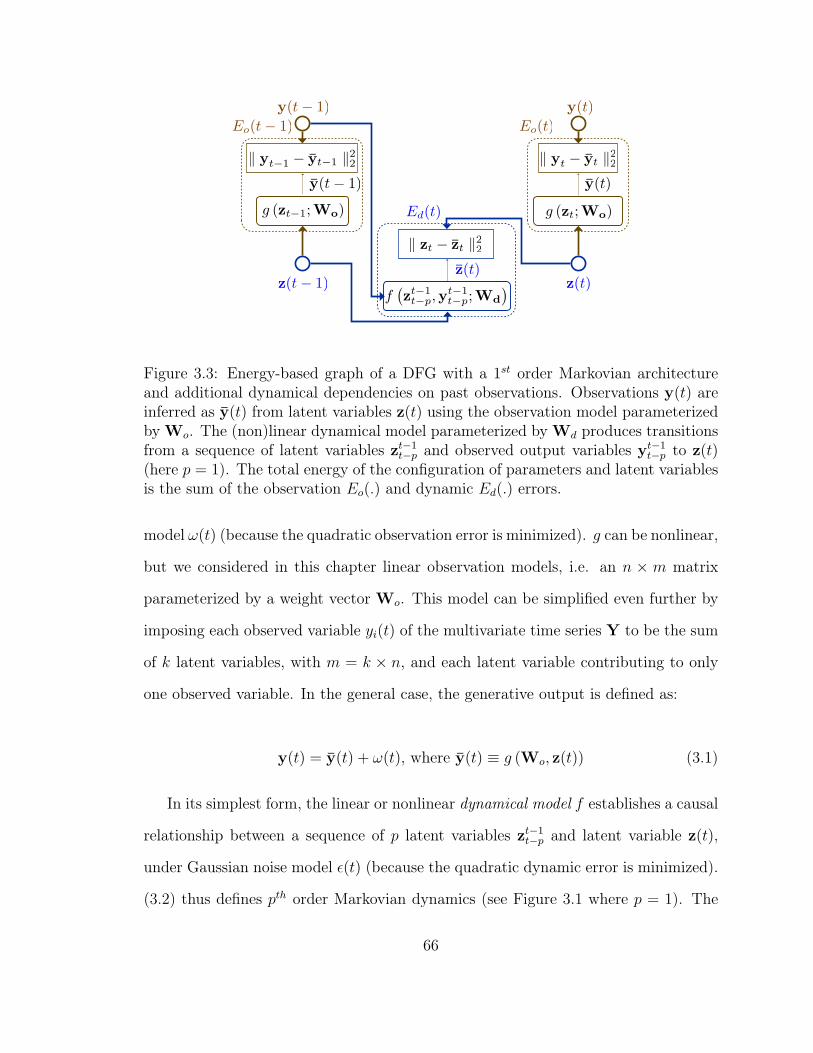
y(t− 1) y(t)

y(t)y(t− 1)

z(t− 1) z(t)z(t)

Ed(t)

Eo(t)Eo(t− 1)

yt−1 − yt−1 22 yt − yt 2

2

zt − zt 22

fzt−1

t−p,yt−1t−p;Wd

g (zt;Wo)g (zt−1;Wo)

Figure 3.3: Energy-based graph of a DFG with a 1st order Markovian architectureand additional dynamical dependencies on past observations. Observations y(t) areinferred as y(t) from latent variables z(t) using the observation model parameterizedby Wo. The (non)linear dynamical model parameterized by Wd produces transitionsfrom a sequence of latent variables zt−1

t−p and observed output variables yt−1t−p to z(t)

(here p = 1). The total energy of the configuration of parameters and latent variablesis the sum of the observation Eo(.) and dynamic Ed(.) errors.

model ω(t) (because the quadratic observation error is minimized). g can be nonlinear,

but we considered in this chapter linear observation models, i.e. an n × m matrix

parameterized by a weight vector Wo. This model can be simplified even further by

imposing each observed variable yi(t) of the multivariate time series Y to be the sum

of k latent variables, with m = k × n, and each latent variable contributing to only

one observed variable. In the general case, the generative output is defined as:

y(t) = y(t) + ω(t), where y(t) ≡ g (Wo, z(t)) (3.1)

In its simplest form, the linear or nonlinear dynamical model f establishes a causal

relationship between a sequence of p latent variables zt−1t−p and latent variable z(t),

under Gaussian noise model ε(t) (because the quadratic dynamic error is minimized).

(3.2) thus defines pth order Markovian dynamics (see Figure 3.1 where p = 1). The

66

dynamical model is parameterized by vector Wd.

z(t) = z(t) + ε(t), where z(t) ≡ f(Wd, z

t−1t−p)

(3.2)

Typically, one can use simple multivariate autoregressive linear functions to map

the state variables, or can also resort to nonlinear dynamics modeled by a Convolu-

tional Network (LeCun et al., 1998a) with convolutions (FIR filters) across time, as

in Time-Delay Neural Networks (Lang and Hinton, 1988; Wan, 1993).

Other dynamical models, different from the Hidden Markov Model, are also pos-

sible. For instance, latent variables z(t) can depend on a sequence of p past latent

variables zt−1t−p and p past observations yt−1

t−p, using the same error term ε(t), as ex-

plained in (3.3) and illustrated on Figure 3.2.

z(t) = z(t) + ε(t), where z(t) ≡ f(Wd, z

t−1t−p,y

t−1t−p)

(3.3)

Figure 3.3 displays the interaction between the observation (3.1) and dynamical

(3.3) models, the observed Y and latent Z variables, and the quadratic error terms.

As will be explained in the next sections, hidden variables Z are initialized ran-

domly, and several priors on their distribution (e.g. bounded representation, sparsity

or smoothness) are incorporated thanks to regularization.

3.2.2 Inference in Dynamic Factor Graphs

Let us define the following total (3.4), dynamical (3.5) and observation (3.6) ener-

gies (quadratic errors) on a given time interval [ta, . . . , tb], where respective weight

coefficients α, β are positive constants (in this chapter, α = β = 0.5):

67

E(Wd,Wo,Y

tbta

)=

tb∑

t=ta

[αEd(t) + βEo(t)] (3.4)

Ed(t) ≡ minZEd(Wd, z

t−1t−p, z(t)

)(3.5)

Eo(t) ≡ minZEo (Wo, z(t), Y (t)) (3.6)

Inferring the sequence of latent variables z(t)t in (3.4) and (3.5) is equivalent to

simultaneous minimization of the sum of dynamical and observation energies at all

times t:

Ed(Wd, z

t−1t−p, z(t)

)= ‖ z(t)− z(t) ‖2

2 (3.7)

Eo (Wo, z(t),y(t)) = ‖ y(t)− y(t) ‖22 (3.8)

Observation and dynamical errors are expressed separately, either as Normalized

Mean Square Errors (NMSE) or Signal-to-Noise Ratio (SNR).

3.2.3 Prediction in Dynamic Factor Graphs

Assuming fixed parameters W of the DFG, two modalities are possible for the pre-

diction of unknown observed variables Y.

• Closed-loop (iterated) prediction: when the continuation of the time series is

unknown, the only relevant information comes from the past. One uses the

dynamical model to predict z(t) from yt−1t−p and inferred zt−1

t−p, set z(t) = z(t),

use the observation model to compute prediction y(t) from z(t), and iterate as

long as necessary. If the dynamics depend on past observations, one also needs

68

to rely on predictions y(t) in (3.3).

• Prediction as inference: this is the case when only some elements of Y are

unknown (e.g. estimation of missing motion-capture data). First, one infers

latent variables through gradient descent, and simply does not backpropagate

errors from unknown observations. Then, missing values yi(t) are predicted

from corresponding latent variables z(t). In this way, we can incorporate a

dependency on future values of the observed time series.

3.2.4 Training of Dynamic Factor Graphs

Learning in an DFG consists in adjusting the parameters W =[WT

d ,WTo

]in order

to minimize the loss L(W,Y, Z):

L(W,Y,Z) = E (W,Y) +Rz(Z) +R (W) (3.9)

Z = arg minZL(W,Y,Z) (3.10)

W = arg minWL(W,Y, Z) (3.11)

where R(W) is a regularization term on the weights Wd and Wo, and Rz(Z) rep-

resents additional constraints on the latent variables further detailed. Minimization

of this loss is done iteratively in an Expectation-Maximization-like fashion in which

the states Z play the role of auxiliary variables, as explained in Chapter 2. During

inference, values of the model parameters are clamped and the hidden variables are

relaxed to minimize the energy. The inference described in part (3.2.2) and equation

(3.10) can be considered as the E-step (state update) of a gradient-based version of

the EM algorithm. During learning, model parameters W are optimized to give lower

69

energy to the current configuration of hidden and observed variables. The parameter-

adjusting M-step (weight update) described by (3.11) is also gradient-based.

In its current implementation, the E-step inference is done by gradient descent

on Z, with learning rate ηz typically equal to 0.5. The convergence criterion is when

energy (3.4) stops decreasing. The M-step parameter learning is implemented as

a stochastic gradient descent (diagonal Levenberg-Marquard) (LeCun et al., 1998b)

with individual learning rates per weight (re-evaluated every 10000 weight updates)

and global learning rate ηw typically equal to 0.01. These parameters were found by

trial and error (cross-validation) on a grid of possible values.

The state inference is not done on the full sequence at once, but on mini-batches

(typically 20 to 100 samples), and the weights get updated once after each mini-batch

inference, similarly to the Generalized EM algorithm. During one epoch of training,

the batches are selected randomly and overlap in such a way that each state variable

Z(t) is re-inferred at least a dozen times in different mini-batches. This learning

approximation echoes the one in regular stochastic gradient with no latent variables

and enables to speed up the learning of the weight parameters.

The learning algorithm turns out to be particularly simple and flexible. The hid-

den state inference is however under-constrained, because of the higher dimensionality

of the latent states and despite the dynamical model. For this reason, this chapter

proposes to (in)directly regularize the hidden states in several ways. First, one can

add to the loss function an L1 regularization term R(W) on the weight parameters.

This way, the dynamical model becomes “sparse” in terms of its inputs, e.g. the latent

states. Regarding the term Rz(Z), an L2 norm on the hidden states z(t) limits their

overall magnitude, and an L1 norm enforces their sparsity both in time and across

dimensions. Regularization coefficients λw and λz typically range from 0 to 0.1.

70

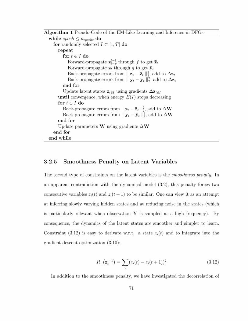
Algorithm 1 Pseudo-Code of the EM-Like Learning and Inference in DFGswhile epoch ≤ nepochs dofor randomly selected I ⊂ [1, T ] dorepeatfor t ∈ I do

Forward-propagate zt−1t−p through f to get zt

Forward-propagate zt through g to get ytBack-propagate errors from ‖ zt − zt ‖2

2, add to ∆ztBack-propagate errors from ‖ yt − yt ‖2

2, add to ∆ztend forUpdate latent states zt∈I using gradients ∆zt∈I

until convergence, when energy E(I) stops decreasingfor t ∈ I do

Back-propagate errors from ‖ zt − zt ‖22, add to ∆W

Back-propagate errors from ‖ yt − yt ‖22, add to ∆W

end forUpdate parameters W using gradients ∆W

end forend while

3.2.5 Smoothness Penalty on Latent Variables

The second type of constraints on the latent variables is the smoothness penalty. In

an apparent contradiction with the dynamical model (3.2), this penalty forces two

consecutive variables zi(t) and zi(t+ 1) to be similar. One can view it as an attempt

at inferring slowly varying hidden states and at reducing noise in the states (which

is particularly relevant when observation Y is sampled at a high frequency). By

consequence, the dynamics of the latent states are smoother and simpler to learn.

Constraint (3.12) is easy to derivate w.r.t. a state zi(t) and to integrate into the

gradient descent optimization (3.10):

Rz

(zt+1t

)=∑

i

(zi(t)− zi(t+ 1))2 (3.12)

In addition to the smoothness penalty, we have investigated the decorrelation of

71

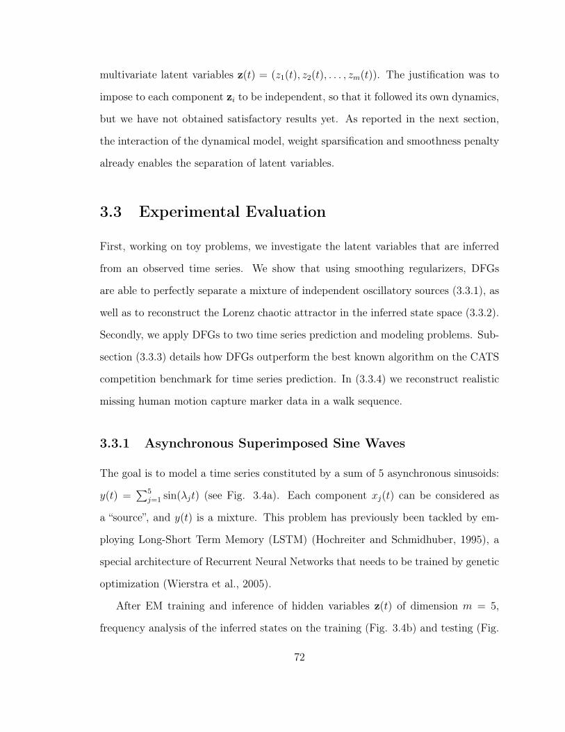
multivariate latent variables z(t) = (z1(t), z2(t), . . . , zm(t)). The justification was to

impose to each component zi to be independent, so that it followed its own dynamics,

but we have not obtained satisfactory results yet. As reported in the next section,

the interaction of the dynamical model, weight sparsification and smoothness penalty

already enables the separation of latent variables.

3.3 Experimental Evaluation

First, working on toy problems, we investigate the latent variables that are inferred

from an observed time series. We show that using smoothing regularizers, DFGs

are able to perfectly separate a mixture of independent oscillatory sources (3.3.1), as

well as to reconstruct the Lorenz chaotic attractor in the inferred state space (3.3.2).

Secondly, we apply DFGs to two time series prediction and modeling problems. Sub-

section (3.3.3) details how DFGs outperform the best known algorithm on the CATS

competition benchmark for time series prediction. In (3.3.4) we reconstruct realistic

missing human motion capture marker data in a walk sequence.

3.3.1 Asynchronous Superimposed Sine Waves

The goal is to model a time series constituted by a sum of 5 asynchronous sinusoids:

y(t) =∑5

j=1 sin(λjt) (see Fig. 3.4a). Each component xj(t) can be considered as

a “source”, and y(t) is a mixture. This problem has previously been tackled by em-

ploying Long-Short Term Memory (LSTM) (Hochreiter and Schmidhuber, 1995), a

special architecture of Recurrent Neural Networks that needs to be trained by genetic

optimization (Wierstra et al., 2005).

After EM training and inference of hidden variables z(t) of dimension m = 5,

frequency analysis of the inferred states on the training (Fig. 3.4b) and testing (Fig.

72

Figure 3.4: (a) Superposition of five asynchronous sinusoids: y(t) =∑5

j=1 sin(λjt)where λ1 = 0.2, λ2 = 0.311, λ3 = 0.42, λ4 = 0.51 and λ5 = 0.74. Spectrum analysisshows that after learning and inference, each reconstructed state zi isolates only oneof the original sources xj, both on the training (b) and testing (c) datasets.

3.4c) datasets showed that each latent state zi(t) reconstructed one individual sinu-

soid. In other words, the 5 original sources from the observation mixture y(t) were

inferred on the 5 latent states. The observation SNR of 64dB, and the dynamical SNR

of 54dB, on both the training and testing datasets, proved both that the dynamics of

the original time series y(t) were almost perfectly reconstructed. DFGs outperformed

LSTMs on that task since the multi-step iterated (closed-loop) prediction of DFG did

not decrease in SNR even after thousands of iterations, contrary to (Wierstra et al.,

2005) where a reduction in SNR was already observed after around 700 iterations.

As architecture for the dynamical model, 5 independent Finite Impulse Response

(FIR) filters of order 25 were chosen to model the state transitions: each of them acts

as a band-pass filter and models an oscillator at a given frequency. One can hypothe-

size that the smoothness penalty (3.12), weighted by a small coefficient of 0.01 in the

state regularization term Rz(Z) helped shape the hidden states into perfect sinusoids.

Note that the states or sources were made independent by employing five independent

dynamical models for each state. This specific usage of DFG can be likened to Blind

Source Separation from an unique source, and the use of independent filters for the

73

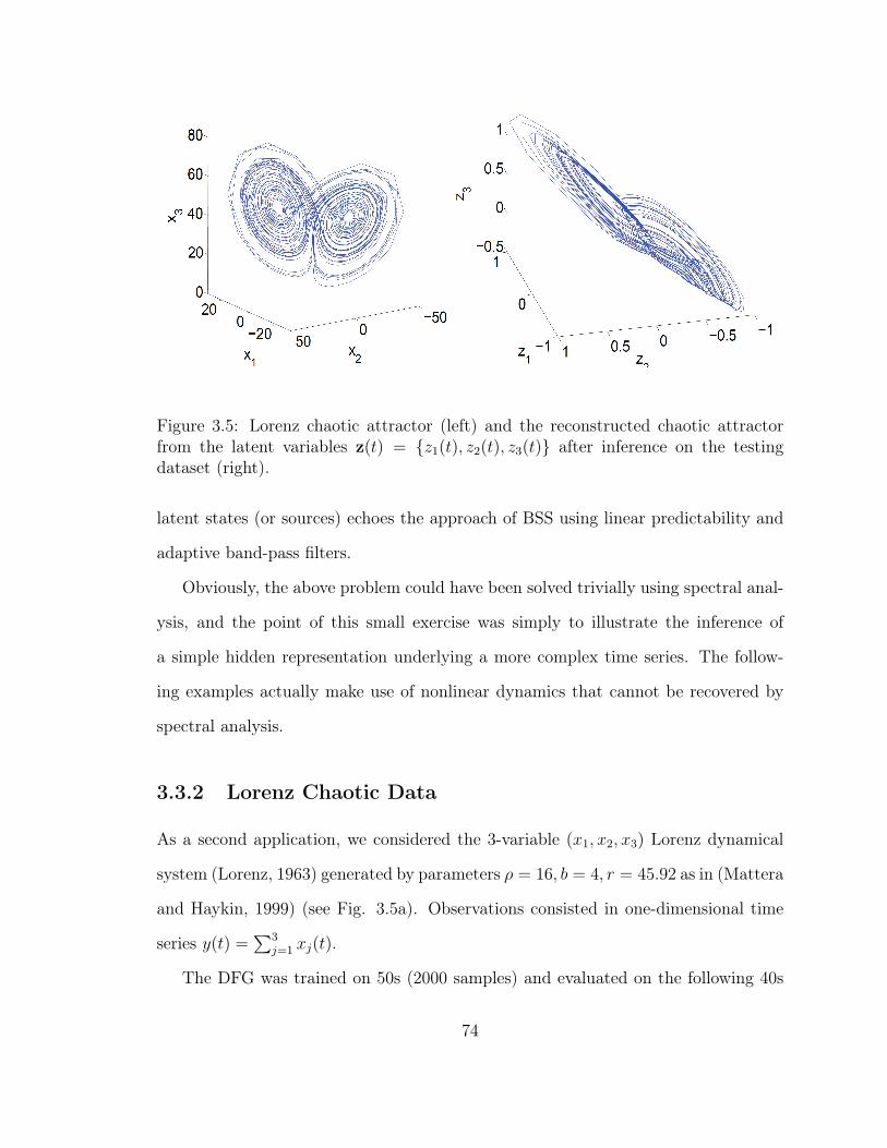
Figure 3.5: Lorenz chaotic attractor (left) and the reconstructed chaotic attractorfrom the latent variables z(t) = z1(t), z2(t), z3(t) after inference on the testingdataset (right).

latent states (or sources) echoes the approach of BSS using linear predictability and

adaptive band-pass filters.

Obviously, the above problem could have been solved trivially using spectral anal-

ysis, and the point of this small exercise was simply to illustrate the inference of

a simple hidden representation underlying a more complex time series. The follow-

ing examples actually make use of nonlinear dynamics that cannot be recovered by

spectral analysis.

3.3.2 Lorenz Chaotic Data

As a second application, we considered the 3-variable (x1, x2, x3) Lorenz dynamical

system (Lorenz, 1963) generated by parameters ρ = 16, b = 4, r = 45.92 as in (Mattera

and Haykin, 1999) (see Fig. 3.5a). Observations consisted in one-dimensional time

series y(t) =∑3

j=1 xj(t).

The DFG was trained on 50s (2000 samples) and evaluated on the following 40s

74

Table 3.1: Comparison of 1-step prediction error using Support Vector Regression,with the errors of the dynamical and observation models of DFGs, measured on theLorenz test dataset and expressed as signal-to-noise ratios.

Architecture SVR DFGDynamic SNR 41.6 dB 46.2 dBObservation SNR - 31.6 dB

(1600 samples) of Y. Latent variables Z(t) = (z1(t), z2(t), z3(t)) had dimension m =

3, as it was greater than the attractor correlation dimension of 2.06 and equal to the

number of explicit variables (sources). The dynamical model was implemented as

a 3-layered convolutional network. The first layer contained 12 convolutional filters

covering 3 time steps and one latent component, replicated on all latent components

and every 2 time samples. The second layer contained 12 filters covering 3 time steps

and all previous hidden units, and the last layer was fully connected to the previous

12 hidden units and 3 time steps. The dynamical model was autoregressive on p = 11

past values of Z, with a total of 571 unique parameters. “Smooth” consecutive states

were enforced (3.12), thanks to the state regularization term Rz(Z) weighted by a

small coefficient of 0.01. After training the parameters of DFG, latent variables Z

were inferred on the full length of the training and testing dataset, and plotted in 3D

values of triplets (z1(t), z2(t), z3(t)) (see Fig. 3.5b).

The 1-step dynamical SNR obtained with a training set of 2000 samples was higher

than the 1-step prediction SNR reported for Support Vector Regression (SVR) (Mat-

tera and Haykin, 1999) (see Table 3.1). According to the Takens theorem (Takens,

1981), it is possible to reconstruct an unknown (hidden) chaotic attractor from an

adequately long window of observed variables, using time-delay embedding on y(t),

but we managed to reconstruct this attractor on the latent states (z1(t), z2(t), z3(t))

inferred both from the training or testing datasets (Fig. 3.5). Although one of the

75

Table 3.2: Prediction results on the CATS competition dataset comparing the bestalgorithm (Kalman Smoothers (Sarkka et al., 2004)) and Dynamic Factor Graphs.E1 and E2 are unnormalized MSE, measured respectively on all five missing segmentsor on the first four missing segments.

Architecture Kalman smoother DFGE1 (5 segments) 4.08 3.90E2 (4 segments) 3.46 2.88

“wings” of the reconstructed butterfly-shaped attractor is slightly twisted, one can

clearly distinguish two basins of attraction and a chaotic orbit switching between one

and the other. The reconstructed latent attractor has correlation dimensions 1.89

(training dataset) and 1.88 (test dataset).

3.3.3 CATS Time Series Competition

Dynamic Factor Graphs were evaluated on time series prediction problems using the

CATS benchmark dataset (Lendasse et al., 2004). The goal of the competition was

the prediction of 100 missing values divided into five groups of 20, the last group being

at the end of the provided time series. The dataset presented a noisy and chaotic

behaviour commonly observed in financial time series such as stock market prices.

In order to predict the missing values, the DFG was trained for 10 epochs on the

known data (5 chunks of 980 points each). 5-dimensional latent states on the full 5000

point test time series were then inferred in one E-step, as described in section 3.2.3.

The dynamical factor was the same as in section 3.3.2. As shown in Table 3.2, the

DFG outperformed the best results obtained at the time of the competition, using a

Kalman Smoother (Sarkka et al., 2004), and managed to approximate the behavior

of the time series in the missing segments.

76

Table 3.3: Reconstruction error (NMSE) for 4 sets of missing joint angles from motioncapture data (two blocks of 65 consecutive frames, about 2s, on either the left legor entire upper body). DFGs are compared to standard nearest neighbors matching.Because of different normalizations, we cannot directly compare our performance tothe one achieved by CRBMs in (Taylor et al., 2006), but in both cases, we observe acomparable reduction in error of the order of 20%.

Method Nearest Neighb. DFGMissing leg 1 0.77 0.59Missing leg 2 0.47 0.39Missing upper body 1 1.24 0.9Missing upper body 2 0.8 0.48

3.3.4 Estimation of Missing Motion Capture Data

Finally, DFGs were applied to the problem of estimating missing motion capture data.

Such situations can arise when “the motion capture process [is] adversely affected by

lighting and environmental effects, as well as noise during recording” (Taylor et al.,

2006). The estimation of missing markers is a difficult problem that was traditionally

handled using simple algorithmic solutions, such as nearest neighbors, piece-wise lin-

ear modeling (Liu and McMillan, 2006), or Kalman Filtering (Aristidou et al., 2008).

Motion capture data1 Y consisted of three 49-dimensional time series representing

joint angles derived from 17 markers and coccyx, acquired on a subject walking and

turning, and downsampled to 30Hz. Two sequences of 438 and 3128 samples were

used for training, and one sequence of 260 samples for testing.

We reproduced the experiments from (Taylor et al., 2006), where Conditional

Restricted Boltzman Machines (CRBM) were utilized. On the test sequence, two

different sets of joint angles were erased, either the left leg (1) or the entire upper1We used motion capture data from the MIT database as well as sample Matlab code for motion

playback and conversion, developed or adapted by Taylor, Hinton and Roweis, available at: http://www.cs.toronto.edu/~gwtaylor/.

77

body (2). After training the DFG on the training sequences, missing joint angles

yi(t) were inferred through the E-step inference. The DFG was the same as in sec-

tions 3.3.2 and 3.3.3, but with 147 hidden variables (3 per observed variable) and no

smoothing. Table 3.3 shows that DFGs significantly outperformed nearest neighbor

interpolation (detailed in (Taylor et al., 2006)), by taking advantage of the motion dy-

namics modeled through dynamics on latent variables. Contrary to nearest neighbors

matching, DFGs managed to infer smooth and realistic leg or upper body motion.

Videos comparing the original walking motion sequence, and the DFG- and nearest

neighbor-based reconstructions are available at

http://cs.nyu.edu/~mirowski/pub/mocap/. Figure 3.6 illustrates the DFG-based

reconstruction (we did not include nearest neighbor interpolation resuts because the

reconstructed motion was significantly more “hashed” and discontinuous).

3.4 Discussion

In this section, we establish a comparison with other nonlinear dynamical systems

with latent variables (3.4.1) and suggest that DFGs could be seen as an alternative

method for training Recurrent Neural Networks (3.4.2).

3.4.1 Comparison with Nonlinear Dynamical Systems

An earlier model of nonlinear dynamical system with hidden states is the Hidden

Control Neural Network (Levin, 1993), where latent variables z(t) are added as an

additional input to the dynamical model on the observations. Although the dynam-

ical model is stationary, the latent variable z(t) modulates its dynamics, enabling a

behavior more complex than in pure autoregressive systems. The training algorithm

iteratively optimizes the weights W of the Time-Delay Neural Network (TDNN) and

78

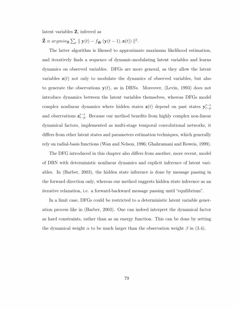
latent variables Z, inferred as

Z ≡ argminZ

∑t ‖ y(t)− fW (y(t− 1), z(t)) ‖2.

The latter algorithm is likened to approximate maximum likelihood estimation,

and iteratively finds a sequence of dynamic-modulating latent variables and learns

dynamics on observed variables. DFGs are more general, as they allow the latent

variables z(t) not only to modulate the dynamics of observed variables, but also

to generate the observations y(t), as in DBNs. Moreover, (Levin, 1993) does not

introduce dynamics between the latent variables themselves, whereas DFGs model

complex nonlinear dynamics where hidden states z(t) depend on past states yt−1t−p

and observations zt−1t−p. Because our method benefits from highly complex non-linear

dynamical factors, implemented as multi-stage temporal convolutional networks, it

differs from other latent states and parameters estimation techniques, which generally

rely on radial-basis functions (Wan and Nelson, 1996; Ghahramani and Roweis, 1999).

The DFG introduced in this chapter also differs from another, more recent, model

of DBN with deterministic nonlinear dynamics and explicit inference of latent vari-

ables. In (Barber, 2003), the hidden state inference is done by message passing in

the forward direction only, whereas our method suggests hidden state inference as an

iterative relaxation, i.e. a forward-backward message passing until “equilibrium”.

In a limit case, DFGs could be restricted to a deterministic latent variable gener-

ation process like in (Barber, 2003). One can indeed interpret the dynamical factor

as hard constraints, rather than as an energy function. This can be done by setting

the dynamical weight α to be much larger than the observation weight β in (3.4).

79

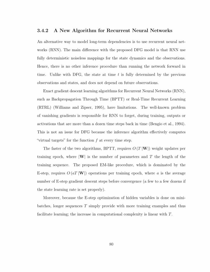
3.4.2 A New Algorithm for Recurrent Neural Networks

An alternative way to model long-term dependencies is to use recurrent neural net-

works (RNN). The main difference with the proposed DFG model is that RNN use

fully deterministic noiseless mappings for the state dynamics and the observations.

Hence, there is no other inference procedure than running the network forward in

time. Unlike with DFG, the state at time t is fully determined by the previous

observations and states, and does not depend on future observations.

Exact gradient descent learning algorithms for Recurrent Neural Networks (RNN),

such as Backpropagation Through Time (BPTT) or Real-Time Recurrent Learning

(RTRL) (Williams and Zipser, 1995), have limitations. The well-known problem

of vanishing gradients is responsible for RNN to forget, during training, outputs or

activations that are more than a dozen time steps back in time (Bengio et al., 1994).

This is not an issue for DFG because the inference algorithm effectively computes

“virtual targets” for the function f at every time step.

The faster of the two algorithms, BPTT, requires O (T |W|) weight updates per

training epoch, where |W| is the number of parameters and T the length of the

training sequence. The proposed EM-like procedure, which is dominated by the

E-step, requires O (aT |W|) operations per training epoch, where a is the average

number of E-step gradient descent steps before convergence (a few to a few dozens if

the state learning rate is set properly).

Moreover, because the E-step optimization of hidden variables is done on mini-

batches, longer sequences T simply provide with more training examples and thus

facilitate learning; the increase in computational complexity is linear with T .

80

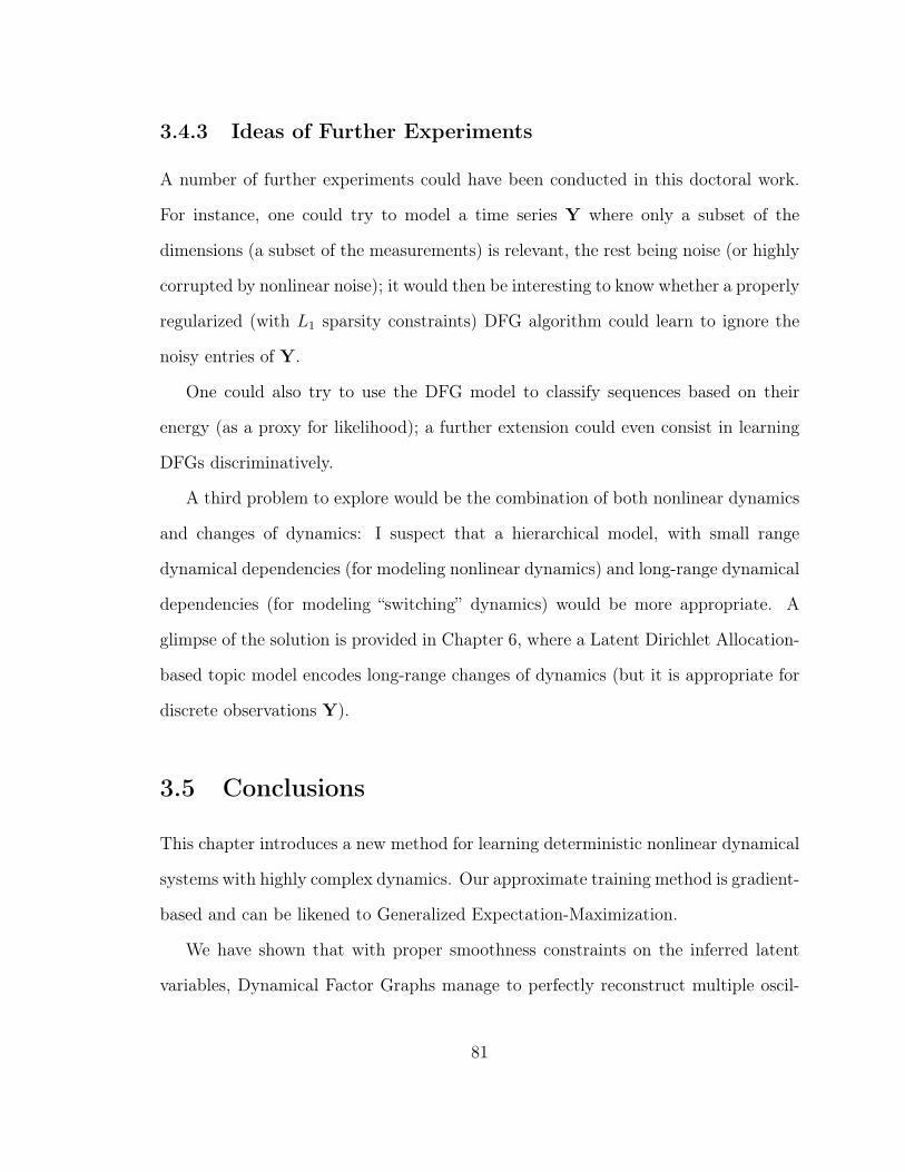
3.4.3 Ideas of Further Experiments

A number of further experiments could have been conducted in this doctoral work.

For instance, one could try to model a time series Y where only a subset of the

dimensions (a subset of the measurements) is relevant, the rest being noise (or highly

corrupted by nonlinear noise); it would then be interesting to know whether a properly

regularized (with L1 sparsity constraints) DFG algorithm could learn to ignore the

noisy entries of Y.

One could also try to use the DFG model to classify sequences based on their

energy (as a proxy for likelihood); a further extension could even consist in learning

DFGs discriminatively.

A third problem to explore would be the combination of both nonlinear dynamics

and changes of dynamics: I suspect that a hierarchical model, with small range

dynamical dependencies (for modeling nonlinear dynamics) and long-range dynamical

dependencies (for modeling “switching” dynamics) would be more appropriate. A

glimpse of the solution is provided in Chapter 6, where a Latent Dirichlet Allocation-

based topic model encodes long-range changes of dynamics (but it is appropriate for

discrete observations Y).

3.5 Conclusions

This chapter introduces a new method for learning deterministic nonlinear dynamical

systems with highly complex dynamics. Our approximate training method is gradient-

based and can be likened to Generalized Expectation-Maximization.

We have shown that with proper smoothness constraints on the inferred latent

variables, Dynamical Factor Graphs manage to perfectly reconstruct multiple oscil-

81

latory sources or a multivariate chaotic attractor from an observed one-dimensional

time series. DFGs also outperform Kalman Smoothers and other neural network tech-

niques on a chaotic time series prediction tasks, the CATS competition benchmark.

Finally, DFGs can be used for the estimation of missing motion capture data. Proper

regularization such as smoothness or a sparsity penalty on the parameters enable to

avoid trivial solutions for high-dimensional latent variables.

This initial work on DFG was subsequently applied to the inference of genetic reg-

ulatory networks from mRNA expression levels, which is the object of next chapter.

82

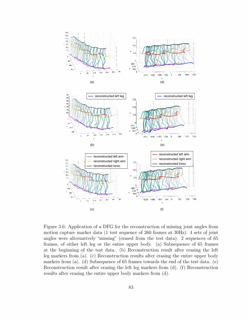
Figure 3.6: Application of a DFG for the reconstruction of missing joint angles frommotion capture marker data (1 test sequence of 260 frames at 30Hz). 4 sets of jointangles were alternatively “missing” (erased from the test data): 2 sequences of 65frames, of either left leg or the entire upper body. (a) Subsequence of 65 framesat the beginning of the test data. (b) Reconstruction result after erasing the leftleg markers from (a). (c) Reconstruction results after erasing the entire upper bodymarkers from (a). (d) Subsequence of 65 frames towards the end of the test data. (e)Reconstruction result after erasing the left leg markers from (d). (f) Reconstructionresults after erasing the entire upper body markers from (d).

83

Chapter 4

Application to the Inference of Gene

Regulation Networks

Time flies like an arrow;

fruit flies like a banana.

Groucho Marx

We present in the chapter how Dynamic Factor Graphs can be used in molecular

biology, as a new and flexible algorithm for learning state-space models represent-

ing gene regulation networks. In one embodiment, our factor graph model contains

observation (transcriptional) and dynamic factors, connected to two types of vari-

ables: observed mRNA expression levels, and hidden transcription factor sequences

(e.g. protein concentrations). In a second embodiment, the latent variables simply

correspond to a de-noised version of the observed mRNA expression levels, and we

try to model dynamics on idealized hidden variables instead of noisy mRNA.

Our formalisms covers most state-space models in the biological literature, while

giving them a common learning and inference procedure that is simpler and faster than

MCMC, Variational Bayes approaches for Dynamic Bayesian Networks and Gaussian

Processes. Learning our factor graphs is still done by maximizing their joint likeli-

84

hood, but we use an approximate gradient-based MAP inference to obtain the most

likely configuration of the hidden sequence.

Our biological state-space model has been applied to two different studies, one

about reverse-engineering a gene regulation network by understanding gene-gene in-

teractions, and another about inferring levels of protein transcription factors, which

are typically difficult to measure, using only mRNA data.

The first set of experiments, submitted for publication to Genome Biology (Krouk

et al., Provisionally accepted for publication), focuses on NO3−, a nitrogen source and

a signaling molecule that controls many aspects of plant development. We try to learn

a gene network involved in plant adaptation to fluctuating nitrate environments, and

specifically to build core regulatory networks involved in Arabidopsis root adaptation

to NO3− provision. Our experimental approach is to monitor genome response to

NO3− at 7 time points, using micro-array chips. A state-space model inferred from

the micro-array data successfully predicted gene behavior in unlearnt conditions, and

suggested to investigate a specific gene, that was then shown to be involved in the

NO3− response.

In a second set of experiments, we demonstrate our algorithm on several datasets:

the p53 protein dataset (related to human cancer), the Mef2 protein from theDrosophila

and the TGF-β protein (human cancer). We show that our algorithm is able the infer

the time course of a single or multiple transcription factor proteins.

85

4.1 Machine Learning Approaches to Modeling GRNs

4.1.1 Gene Regulatory Networks

An excellent biological definition for our problem is provided by (Segal et al., 2003).

“The complex functions of a living cell are carried out through the concerted activity of

many genes [...]. This activity is often coordinated by the organization of the genome

into regulatory modules, or sets of co-regulated genes [...]”. Genes encode proteins,

and the proteins themselves serve as transcription factors to other genes. One of the

goals of modern molecular biology is to identify the interactions between genes (via

proteins) in order to understand, now that the genome has been sequenced, the actual

functioning of the living organisms.

In that context, one can grossly simplify the highly complex biology by a Ge-

netic Regulatory Network (GRN), which can be formalized by a graph connecting

gene, mRNA or protein nodes, and where the links among nodes stand for regulatory

interactions (Alvarez-Buylla et al., 2007).

4.1.2 mRNA Micro-arrays

The tool of choice are so-called gene chips, or DNA micro-arrays. Micro-arrays cor-

respond to small, organism-specific, collections of tiny probes that can bind mRNA1.

Each probe corresponds to a specific gene. After the hybridization process, the

micro-arrays are scanned to measure the concentration of bound mRNA at each

probe (Krouk, personal communication). By conducting specific experiments (e.g.

response to stress conditions, cell development and differentiation), one can initiate a

regulatory circuit (Spellman et al., 1998). Then, by destructively sampling microarray1Standard micro-arrays are the Affymetrix chips.

86

data every few minutes of the experiment, one can obtain a short, high-dimensional

time series of expression levels for thousands of genes. Using the assumption that

the temporal behavior of the multivariate time series represents causal dependencies

between the time series, we can search for protein-encoding transcripts in the genome.

The mRNA time series are typically extremely short (a few measures, sampled

every few minutes to hours). This short duration is a major limitation, given the

number of genes. Moreover, each micro-array experiment is destructive, and therefore

the cells which are sampled at consecutive time points are not the same (Krouk,

personal communication). Each sampling experiment is however repeated a few times,

and one gene expression level has several replicates differing slightly in their value.

Often, the reported gene expression level is the average of these replicates, but one

can consider the replicates separately. Using replicates, one can artificially multiply

the number of microarray time series to obtain more sequences, hence more time

points (Shasha, personal communication).

4.1.3 Reverse-engineering of Gene Regulation Networks

Time series of gene expression levels can provide us with a detailed picture of the

behavior of a Genetic Regulation Network (GRN) over time, and help understand

the biological functions of an organism.

Unfortunately, the micro-array measurements of mRNA expression levels contain

highly noisy, scarce, and incomplete information. Typically, the concentration levels

of proteins, which serve as transcription factors to genes, are absent because they

are difficult to measure. Moreover, their specific influence on genes is unknown and

requires reverse engineering (Jaeger and Monk, 2010). In their review article, Jaeger

and Monk pointed out that this reverse-engineering task in the presence of few time-

87

point measurements, many genes, measurement errors and random fluctuations in the

environment is inherently difficult (Jaeger and Monk, 2010), the main limitation com-

ing from the paucity of data relative to the number of possible connections between

the genes (and the proteins).

An additional challenge of systems biology is to be able to model systems pre-

cisely enough that the model can predict untested conditions, which is equivalent to

constructing a robust dynamical system.

Dynamical Predictive Modeling of Regulatory Gene Networks

Among the several approaches to this modeling problem, dynamical models have

gained prominence as they simultaneously encode the topology of the gene interaction

graph, and its functional evolution model. Such a model can in turn also be used for

predictive modeling of gene expression at further time steps or upon perturbation.

These dynamical models essentially consist of a mathematical function that gov-

erns the transitions of the state of a GRN over time. Interactions between genes and

transcription factors (e.g. proteins) can be simplified as a dynamical model involving

their concentration levels. Typically, dynamical models of mRNA levels consist of

ordinary differential equations (ODEs) (Jaeger and Monk, 2010). For a given gene i,

ODEs can, for instance, define the rate of change of mRNA level yi(t) as a function

of the weighted influences of M transcription factors zj(t), with an optional mRNA’s

degradation term (coefficient di) and a basal rate term (coefficient b), as in Equa-

tion (4.1). The coefficient of the degradation term can be replaced with a kinetic

constant τi on the derivative on yi(t), as in Equation (4.2).

88

∂yi(t)

∂t= gi (z(t))− diyi(t) + bi (4.1)

τ∂yi(t)

∂t= gi (z(t))− yi(t) + bi (4.2)

In the equations above, the transcription factors zt can be the unknown protein

levels, or in a very simplistic setting, other mRNA levels (in which case zt = yt).

In one set of experiments (on p53, Mef2 and TGF-β proteins), we used zt to model

unknown protein levels, while in another set of experiments on the Arabidopsis, we

directly used the observed mRNA levels. In the case of protein transcription factors,

the relationship between a protein zi(t) and its encoding gene yi(t) is generally mod-

eled as a first-order ODE involving zi(t) and yi(t): hence, assuming zt = yt is not

terribly wrong.

In our studies, we considered dynamics with the mRNA degradation term (the

so-called kinetic model (Bonneau et al., 2006, 2007)) and without it (the so-called

Brownian motion (Wang et al., 2006b) model). Assuming degradation (kinetic ODE)

worked better in our experiments with the Arabidopsis.

Since micro-array data are discretely sampled over time, Equation (4.1) or (4.2) is

linearized; hence it explains how gene expressions at time t influence gene expressions

at time t+ 1.

The data paucity limitation defined two major groups of methods for compu-

tational inference of gene regulation networks: a) either a nonlinear or state-space

based modeling of the complex interactions between a restricted number of genes with

hidden protein transcription factors, or b) simpler, but linear, models of TF-gene in-

teractions (Bonneau et al., 2006, 2007; Wang et al., 2006b; Shimamura et al., 2009),

relying on larger (hundreds to thousands) number of mRNA micro-array measure-

89

ments2.

Hidden Variable Approaches: State-Space Models

State-space models (SSM) are a general category of machine learning algorithms

that model the dynamics of a sequence of data by encoding the joint likelihood of

observed Y and hidden Z variables. State-space models assume an observed sequence

y(t) (in our case, gene expression data) to be generated from an underlying unknown

sequence z(t) also called “hidden states”. Consecutive hidden states form a Markov

chain z(1), . . . , z(T − 1), z(T ).

A popular probabilistic example of state-space models that have been applied to

gene expression data are Dynamical Bayesian Networks (Murphy and Mian, 1999)

such as Linear Dynamical Systems (Beal et al., 2005; Hirose et al., 2008; Rangel

et al., 2004; Yamaguchi et al., 2007, 2010; Angus et al., 2010). Examples of such

LDS , are (Beal et al., 2005) and (Angus et al., 2010) who infered the profiles of 14

hidden transcription factors for 10 observed genes. Their modeling was however done

either without predictive validation (Beal et al., 2005), or on synthetically generated

data (Angus et al., 2010). Other researchers (Hirose et al., 2008; Yamaguchi et al.,

2007, 2010) used a trainable Kalman smoother-like approach to learn 4 to 5 hidden

variables (so-called modules) explaining the behavior of hundreds of genes, but neither

validated their model on out-of-sample data points, nor drew conclusions on gene-gene

interactions.

LDS also suffer from their linearity, and may be insufficient to model the nonlin-2In the above enumeration, we actually omitted one group of methods that consist in highly

nonlinear Boolean Networks with binary ON/OFF values for gene expression levels, and linear,nonlinear or stochastic dynamics (Lahdesmaki et al., 2003; Alvarez-Buylla et al., 2007). In suchboolean networks, one typically starts from a hypothesis on the GRN, and then simulates thedynamics of a boolean network, looking for attractors. The objective does not consist in fittingmRNA expression levels.

90

ear regulation of genes by proteins; whereas the derivation of the variational Bayes

solution to nonlinear dynamical systems might be difficult.

Hidden Variable Approaches: Gaussian Processes

The other main approaches devised to solve the ODEs involved in gene regulation

networks consists in Gaussian Processes (GPs) (Lawrence and Sanguinetti, 2007; Gao

et al., 2008; Alvarez et al., 2009), which model the latent protein concentration as a

latent function zj(t) that follows a Gaussian prior with a specified covariance.

That model was further improved in (Zhang et al., 2010), using Gaussian Process

Latent Variable models (Wang et al., 2006a) to infer the profile of a single transcrip-

tion factor (the tumor suppressor p53) and explained the activity of a large collection

of genes using that TF only. GPs however require to analytically derive the covariance

function and can be computationally expensive.

Large-Scale Linear Models Without Hidden Variables

Because the SSM or GP models described in the previous sections can prove com-

putationally expensive and define too many degrees of freedom w.r.t. available data,

the simplification “mRNA = transcription factor” is often used, and a simple linear

model is employed.

Examples of first-order linear dynamical models on gene expressions include the

Inferelator by (Bonneau et al., 2006, 2007). The Inferelator consists of a kinetic

ODE, that follows the Wahde and Hertz equation (Wahde and Hertz, 2001) and

where transcription factors contribute linearly. This ODE also includes an mRNA

degradation term. Some instances of the Inferelator introduce nonlinear AND, OR

and XOR relationships between pairs of genes, based on a previous bi-clustering of

genes. One has to note that the Inferelator has been mostly applied to datasets with

91

hundreds of data-points (e.g. the Halobacterium).

Other examples include the first-order vector autoregressive models VAR(1) (Shi-

mamura et al., 2009), or the Brownian motion (which is a VAR(1) model on the

change of the mRNA concentration (Wang et al., 2006b)). Lozano et al. suggested

using a dynamic dependency on the past 2, 3, or 4 time-steps (Lozano et al., 2009),

but this was impractical in our case given the relatively small number of micro-array

measurements in our experiments.

4.1.4 Biological Datasets Used in Our Experiments

Arabidopsis Thaliana’s Response to NO3−

This research, from the hypothesis and experimental protocol through the experi-

mental manipulation and data analysis, was devised and conducted by Dr. Gabriel

Krouk, at the time post-doctoral researchers in Prof. Gloria Coruzzi’s3 Plant Sys-

tems Biology lab4 at the NYU Center for Genomics and Systems Biology at New

York University. Additional feedback about GRN inference was provided from the

author and from Prof. Dennis Shasha.

Higher plants constitute a main entry of nitrogen in food chains, and acquire nitro-

gen mainly as NO3−. Soil concentration of this mineral ion can fluctuate dramatically

in the rhizosphere, often resulting in limited growth and yield. Thus, understanding

plant adaptation to fluctuating nitrogen levels is a challenging task with potential

consequences for health, the environment, and economy (Krouk et al., 2010).

The first genomic approaches studying NO3− responses were published 10 years

ago (Wang et al., 2000). To date, data from more than 100 Affymetrix ATH1 chips

have been published that monitor gene expression in response to NO3− provision.3Research page at: http://biology.as.nyu.edu/object/GloriaCoruzzi.html4http://coruzzilab.bio.nyu.edu/home/

92

Analysis of the N-treated microarray data sets from several different labs demon-

strated that at least a tenth of the genome can be regulated by nitrogen provision,

depending on the context (Gutierrez et al., 2007). Despite these extensive efforts of

characterization, only a limited number of molecular actors that alter NO3− induced

gene regulation have been identified so far.

In this study, our aim was to provide a systems view of NO3− signal propagation

though dynamic regulatory gene networks. To do so, a high-resolution dynamic NO3−

transcriptome from plants treated with nitrate from 0 to 20 min was generated. The

micro-arrays contained 7 full-genome mRNA measures at 0, 3, 6, 9, 12, 15 and 20 min;

in the cross-validation leave-out-last study, we used measures between 0 and 15 min

to fit the model for each gene i (by tuning the parameters of associated dynamical

functions), and tested the fitted model on the last time step (prediction of the mRNA

level at 20 min).

Two micro-array replicates were acquired in this study, listed in Table 4.1. Since

each replicate is independent of all micro-arrays preceding and following in time,

there were four possible transitions between any two time points t and t+ 1, and we

therefore used 4 replicate sequences to train the machine learning algorithm.

p53, Mef2 and TGF-β Protein Datasets

Our first dataset consisted in the p53 human genome data from (Barenco et al., 2006).

p53 is a “tumor repressor activated during DNA damage. [...] Irradiation is performed

to disrupt the equilibrium of the p53 network stimulating transcription of p53 target

genes. Seven samples [of mRNA] in three replicas [were] collected as the raw time

course data” (Gao et al., 2008)5. Previous studies on that dataset included (Barenco5We used both the pre-processes data available at Neil Lawrence’s website:

http://staffwww.dcs.shef.ac.uk/people/N.Lawrence/software.html, and the raw mRNA associ-ated to the experiment conducted by (Barenco et al., 2006), and available as supplemental

93

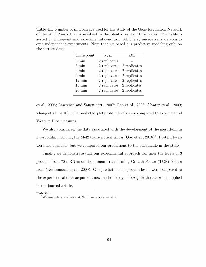
Table 4.1: Number of microarrays used for the study of the Gene Regulation Networkof the Arabidopsis that is involved in the plant’s reaction to nitrates. The table issorted by time-point and experimental condition. All the 26 microarrays are consid-ered independent experiments. Note that we based our predictive modeling only onthe nitrate data.

Time-point NO3− KCl

0 min 2 replicates -3 min 2 replicates 2 replicates6 min 2 replicates 2 replicates9 min 2 replicates 2 replicates12 min 2 replicates 2 replicates15 min 2 replicates 2 replicates20 min 2 replicates 2 replicates

et al., 2006; Lawrence and Sanguinetti, 2007; Gao et al., 2008; Alvarez et al., 2009;

Zhang et al., 2010). The predicted p53 protein levels were compared to experimental

Western Blot measures.

We also considered the data associated with the development of the mesoderm in

Drosophila, involving the Mef2 transcription factor (Gao et al., 2008)6. Protein levels

were not available, but we compared our predictions to the ones made in the study.

Finally, we demonstrate that our experimental approach can infer the levels of 3

proteins from 70 mRNAs on the human Transforming Growth Factor (TGF) β data

from (Keshamouni et al., 2009). Our predictions for protein levels were compared to

the experimental data acquired a new methodology, iTRAQ. Both data were supplied

in the journal article.

material.6We used data available at Neil Lawrence’s website.

94

4.2 Gradient-Based Biological State-Space Models

We propose a new and simple algorithm for learning SSMs representing gene reg-

ulation networks, that can incorporate nonlinear protein-gene interactions or focus

on gene-gene interactions. It is grounded in the factor graph formalism (Kschischang

et al., 2001), which expresses the joint likelihood of the hidden and observed variables

as a product of likelihoods at each factor. Our SSM includes two types of factors: ob-

servation and dynamic factors, which may be connected to two types of variables:

observed mRNA expression levels, and hidden transcription factor sequences (ei-

ther transcription factors, e.g. protein concentrations, or a noise-free time-course

of mRNA), as illustrated respectively on Figure 4.2 or on Figure 4.1.

A “Plug-And-Play” Architecture for SSMs

Our model is flexible because one can essentially ”plug-and-play” different types of fac-

tors to suit various types of SSMs in the biological literature. Each factor is expressed

in the negative log domain, and computes an energy value that can be interpreted as

the negative log likelihood of the configuration of the variables it connects with. The

total energy of the system is the sum of the factors’ energies, so that the maximum

likelihood configuration of variables can be obtained by minimizing the total energy.

Learning our factor graphs is still done by maximizing their joint likelihood, but we

use an approximate gradient-based MAP inference to obtain the most likely config-

uration of the hidden sequence. Such approximate approaches have been applied on

chaotic and motion capture time series modeling problems (Mirowski and LeCun,

2009). Our algorithm is also faster than MCMC or Variational Bayes approaches for

Dynamic Bayesian Networks and than Gaussian Processes.

95

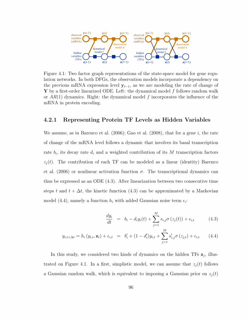
observation model h

z(t-1) z(t) z(t+1)

y(t-1) y(t) y(t+1)

hidden variables

(TFs)

observed variables(mRNA)

dynamical model f

observation model h

z(t-1) z(t) z(t+1)

y(t-1) y(t) y(t+1)

hidden variables

(TFs)

observed variables(mRNA)

dynamical model f

Figure 4.1: Two factor graph representations of the state-space model for gene regu-lation networks. In both DFGs, the observation models incorporate a dependency onthe previous mRNA expression level yt−1, as we are modeling the rate of change ofY by a first-order linearized ODE. Left: the dynamical model f follows random walkor AR(1) dynamics. Right: the dynamical model f incorporates the influence of themRNA in protein encoding.

4.2.1 Representing Protein TF Levels as Hidden Variables

We assume, as in Barenco et al. (2006); Gao et al. (2008), that for a gene i, the rate

of change of the mRNA level follows a dynamic that involves its basal transcription

rate bi, its decay rate di and a weighted contribution of its M transcription factors

zj(t). The contribution of each TF can be modeled as a linear (identity) Barenco

et al. (2006) or nonlinear activation function σ. The transcriptional dynamics can

thus be expressed as an ODE (4.3). After linearization between two consecutive time

steps t and t + ∆t, the kinetic function (4.3) can be approximated by a Markovian

model (4.4), namely a function hi with added Gaussian noise term εi:

dyidt

= bi − diyi(t) +M∑

j=1

si,jσ (zj(t)) + εi,t (4.3)

yi,t+∆t = hi (yi,t, zt) + εi,t = b′i + (1− d′i)yi,t +M∑

j=1

s′i,jσ (zj,t) + εi,t (4.4)

In this study, we considered two kinds of dynamics on the hidden TFs zj, illus-

trated on Figure 4.1. In a first, simplistic model, we can assume that zj(t) follows

a Gaussian random walk, which is equivalent to imposing a Gaussian prior on zj(t)

96

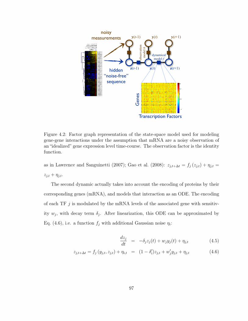
dynamicalmodel fob

serv

atio

nm

odel

h

z(t-1) z(t) z(t+1)

y(t-1) y(t) y(t+1)

Figure 3

Z(t+n)

Predicted behavior

>8

<8

1

KN

O3

/ T

0

Leave-out-two-last 12min ! 15 min ! 20 min

26 consistent genes

Leave-out-last 15 min ! 20 min

53 consistent genes

Learnt set

Learnt set

Predicted behavior

B

C f function: Influence Matrix

Inp

ut

Output

15 ! 20 min

12 ! 15 min

A

Observation model g

Y(t+1) Y(t+n) Y(t) Y(t+2)

Z(t) Z(t+1) Z(t+1)

dynamic model f

KN

O3

/ T

0

Transcription Factors

Gen

es

noisymeasurements

hidden“noise-free”

sequence

Figure 4.2: Factor graph representation of the state-space model used for modelinggene-gene interactions under the assumption that mRNA are a noisy observation ofan “idealized” gene expression level time-course. The observation factor is the identityfunction.

as in Lawrence and Sanguinetti (2007); Gao et al. (2008): zj,t+∆t = fj (zj,t) + ηj,t =

zj,t + ηj,t.

The second dynamic actually takes into account the encoding of proteins by their

corresponding genes (mRNA), and models that interaction as an ODE. The encoding

of each TF j is modulated by the mRNA levels of the associated gene with sensitiv-

ity wj, with decay term δj. After linearization, this ODE can be approximated by

Eq. (4.6), i.e. a function fj with additional Gaussian noise ηi:

dzjdt

= −δjzj(t) + wjyj(t) + ηj,t (4.5)

zj,t+∆t = fj (yj,t, zj,t) + ηi,t = (1− δ′i)zj,t + w′jyj,t + ηj,t (4.6)

97

4.2.2 Representing Noise-Free mRNA as Hidden Variables

In a departure from previous state-space model frameworks, our second approach uses

the hidden variables to represent an idealized, “true” sequence of gene expressions

z(t) that would be measured if there were no noise. The set of all genes at time

t is modeled by a “latent” (i.e., hidden) variable (denoted z(t)), about which noisy

observations y(t) are made. Specifically, we a) model the dynamics on hidden states

z(t) instead of modeling them directly on the Affymetrix data y(t), as well as b) have

the hidden sequence z(t) generate the actual observed sequence y(t) of mRNA, while

incorporating measurement uncertainty. Such an approach has been used in robotics

to cope with errors coming from sensors.

As shown in Figure 4.2, the relationship between consecutive latent variables z(t)

and z(t + 1) is a Markov chain: each latent gene’s expression value at time t + 1 is

assumed to depend only on the state of potentially all the latent gene expressions at

the previous time point t. For each gene i, this relationship stems from the kinetic

ODE involving the rate of mRNA change (with a kinetic time constant τ), mRNA

degradation, and a linear function fi of transcription factor concentrations for that

specific gene. So-called “Brownian motion” dynamics correspond to kinetic dynamics

without the mRNA degradation term. In linearized (discretized) form, the overall

dynamical model f can be represented by an N × M matrix F where N is the

total number of genes and M the number of transcription factors (M ≤ N , and

transcription factors are given indexes from 1 toM), plus a bias term b and a Gaussian

error term with zero mean and fixed covariance:

98

τdzi(t)dt

+ zi(t) = fi (z(t)) + ηi(t) (4.7)

τ

∆t(zi(t+ 1)− zi(t)) + zi(t) =

Ni∑

j=1

Fi,jzj(t) + bi + ηi(t) (4.8)

This linear Markovian model which represents a kinetic (RNA degrades) or Brow-

nian motion (RNA doesnÕt degrade) ODE, is the simplest and requires the fewest

parameters (there is one parameter per TF-gene interaction, and an additional offset

for each target gene). We conjecture that model thus helps to avoid over-fitting scarce

gene data.

The observation model h is essentially an N ×N identity matrix with a Gaussian

error term:

yi(t) = h (zi(t)) + εi(t) (4.9)

yi(t) = zi(t) + εi(t) (4.10)

Because our algorithm is efficient, simple and tractable, as explained in next sec-

tion, it can handle larger numbers of genes (we focussed on 76 genes) than other

state-space model approaches, given enough genes Beal et al. (2005), Angus et al.

(2010), Zhang et al. (2010).

4.2.3 Learning Gradient-Based DFGs

The above functions fi and hj are only a subset of the possible factors that our method

can handle, and they could be substituted by any function that is differentiable with

99

respect to both its parameters and the latent variables. Unlike methods based on

Gaussian Processes Lawrence and Sanguinetti (2007); Alvarez et al. (2009); Zhang

et al. (2010), on expensive MCMC sampling Barenco et al. (2006), or on Variational

Bayes Beal et al. (2005), our method only requires to compute the gradients of all

functions fi and hj, both w.r.t. parameters Θ and w.r.t. latent variables Z.

Expectation-Maximization-Like Coordinate Descent

Learning and inference are performed by minimizing the negative log-likelihood loss

of the factor graph (i.e. is a sum of square errors because of the Gaussian prior on the

error/noise terms). On a sequence Y of T micro-array measurements (including repli-

cate sequences) over N genes, corresponding latent variables Z, under an observation

(and dynamic) models parameterized by Θ, and for given hyperparameters γ (which

controls the weight of the dynamical and observation errors) and λ (for the L1-norm

regularization), the loss is expressed as (4.11). Latent variables Z and parameters Θ

are initialized to small random values. Then the iterative procedure consists of a) the

inference step, where the loss (4.11) is minimized with respect to the latent variables

Z thanks to gradient descent; and of b) the learning step, where the loss (4.11) of

the observation (and dynamical, if relevant) modules is minimized w.r.t. parameters

Θ using conjugate gradient optimization or Least-Angle Regression and Shrinkage

(LARS) if the factor is linear (Tibshirani, 1996). We use small learning rates and

validate the hyperparameters γ and λ on the training data (typically, λ = 0.01 and

γ = 1).

L(Y,Z; Θ, γ, λ) =T∑

t=1

(γ

2

M∑

j=1

η2j,t +

1

2

N∑

i=1

ε2i,t

)+ λ ‖ Θ ‖1 (4.11)

The learning algorithm is run for 100 or 1000 consecutive epochs over all the

100

replicate sequences. In order to retain the optimal set of parameters of f , one selects

the epoch where the dynamic or observation error on the training dataset is minimal.

In the case of model architecture from Section 4.2.2. one run of the learning proce-

dure provides with a matrix F of signed (positive: excitatory or negative: inhibitory)

interactions between transcription factors and genes. Each element Fi,j represents

the action of the j-th transcription factor on the i-th gene.

Hyperparameters and Recovering Existing Methods

Two main hyper-parameters were explored in our learning experiments: the amount of

L1-norm regularization λ (explained in the Methods) and the Lagrange-like coefficient

γ linked to the state-space model. When trying to learn GRN from mRNA (in

Section 4.2.2), we used the kinetic coefficient τ as an additional hyperparameter.

Note that when the state-space coefficient is γ = 0, and using the configuration

from Section 4.2.2), we can recover non-SSM algorithms: (Efron et al., 2004), as used

for instance by Bonneau et al. (Bonneau et al., 2006, 2007) and Elastic Nets (Zou and

Hastie, 2005), as used for instance by Shimamura et al. (Shimamura et al., 2009). In

that case, we simply have Y = Z. Moreover, if we do not use the mRNA degradation

term in the kinetic ODE, and use instead “Brownian motion” dynamics, and if we set

the state-space coefficient to γ = 0, we recover an approach comparable to the one

published by Wang et al. (Wang et al., 2006b) (although their optimization algorithm

was based on the SVD of the micro-array data).

Regularization

During the learning step, sparse gene regulation networks are obtained by penalizing

dense solutions using L1-norm regularization, which amounts to adding a λ-weighted

penalty to the dynamical error term, as in the LASSO initially described by Tibshirani

101

Tibshirani (1996). Employing regularization on parameters also helps avoiding local

optima in the solutions.

LARS is a fast implementation of Tibshirani’s popular LASSO regression with L1-

norm regularization (Tibshirani, 1996). Elastic Nets are an improvement over LARS

and LASSO, and their main advantage is to group variables (in our case genes) as

opposed to choosing one gene and leaving out correlated ones.

Selection of Gene Regulation Network by Bootstrapping

Using a bootstrapping approach based on random initialization of latent variables

z(t), we further repeat the SSM iterative procedure 20 times and take the final average

model.

In the case of the dynamical model on noise-free mRNA described in Section 4.2.2,

we use bootstrapping to determine the statistically significant gene-gene links. The

above-explained algorithm for learning state-space models starts with random initial

values for both the dynamical model (in other words, matrix F) and for the latent

variables Z. We repeat the whole procedure 20 times in order to perform the following

bootstrapping evaluation. Each run k of the algorithm might converge to a slightly dif-

ferent solution F∗(k). We then take the average TF-gene interactions weights obtained

from all solutions F∗(k) and call it F∗. The table on Figure 4.4 reports comparative

results on the average solutions. In parallel, we also generate 1000 random permuta-

tions of each matrix F∗(k), defined respectively as P∗(k, 1),P∗(k, 2), . . . ,P∗(k, 1000),

and then compute 1000 average matrices P∗(1),P∗(2), . . . ,P∗(1000) of those “scram-

bled” matrices (we take the averages over the 20 runs). We compare each average

element F ∗i,j to the empirical distribution of the 1000 permuted averages and thus ob-

tain an empirical p-value. The final genetic regulation network consists in elements

F ∗i,j that have a p-value p < 0.001.

102

4.3 GRN of the Arabidopsis Response to NO3−

In this study, instead of learning the dynamics directly on the gene expression se-

quence, we took into account uncertainty and acquisition errors, and used a state-

space model. The latter defined the observed gene expression time series (denoted as

y(t)) as being generated by a hidden “true” sequence of gene expressions z(t). This

approach enabled us to both incorporate uncertainty about the measured mRNA and

to model the gene regulation network by simple linear dynamics on the hidden vari-

ables (so-called “states”), thus reducing the number of (unknown) free parameters and

the associated risk of over-fitting the observed data.

Our DFG-based method delivered a coherent regulatory model that was good

enough to predict the direction of gene change (up regulation or down regulation) on

future data points. This coherence allowed us to propose a gene influence network

involving transcription factors and “sentinel genes” involved in the primary NO3− re-

sponse (such as NO3− transporters or NO3− assimilation genes). The role of a predicted

hub in this network was evaluated in further biological experiments by over-expressing

it, and indeed lead to changes in the NO3− driven gene expression of sentinel genes.

4.3.1 Comparative Study of State-Space Model Optimization

Out of the 550 N-regulated genes we extracted 67 genes which correspond to all

the predicted transcription factors and 9 N-regulated genes that belonged to the N-

assimilation pathway (including sentinel genes). Their mRNA over 7 time points and

for 2 replicates is shown on Figure 4.3. The transcription factors have been used

as explanatory variables (inputs to f) as well as explained values (output from f),

whereas the N-assimilation genes are only explained values. We then optimized the

103

Figure 3

Figure 4.3: 76-gene micro-array used for the Arabidopsis study. The last time-point,corresponding to time t = 20 min, was out-of-sampled and used for evaluating thepredictive capability of our dynamical model of gene regulation.

state-space model, using different algorithms, in order to fit it to the observed data

matrix, and compared all our results in the table on Figure 4.4. We also compared

our SSM approach to non-SSM approaches (Bonneau et al., 2006, 2007; Wang et al.,

2006b; Efron et al., 2004; Zou and Hastie, 2005; Shimamura et al., 2009) in in the

table on Figure 4.5.

For each type of ODE (kinetic or “Brownian motion”) and type of optimization

algorithm, we exhaustively explored the space of hyper-parameters (γ, λ, ρ) in order

to optimize the quality of fit of each model to the first six time-points (0 min, 3 min,

6 min, 9 min, 12 min and 15 min). As can be seen in the table on Figure 4.4, we

identified the state-space model relying on the kinetic ODE, and with either LARS or

conjugate gradient optimizations, as the two best (having the highest Signal-to-Noise

Ratio (SNR)) optimization algorithms on the MAS5 training datasets. The signal-to-

104

!"#$%&'(")

*%+,-.

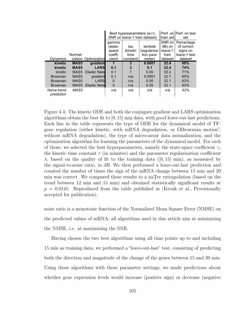
/0)%#'1( 2$3'#'4%3'")

!"#$%"& '()* +,-."$#% / 0 12111/ 0324 567

!"#$%"& '()* 8(9) 12/ 0 12/ 0324 :47

5'),3'1 6789 :;%(3'1-<,3( =>. ? =>=9 @A>A ?.B

C&"D)'%) 6789 +&%E',)3 =>. )F% =>===. @A>. G9B

C&"D)'%) 6789 H7I8 = )F% =>=9 @A>. G@B

C&"D)'%) 6789 :;%(3'1-<,3( = )F% =>=9 @A>. G@B

!"#$ %&' %&' %&' %&' $()

C,(3-J0$,&$%&%#,3,&(-KD>&>3>-8<I-")-;,%L,M.-3&%')-E%3%(,3N

*,&O>-")-3&%')-(,3

*,&O>-")-3,(3-(,3

<"&#%;M'4%3'")

+%##%-K(3%3,M($%1,-1",OO'M1',)3N

3%P-K5'),3'1-3'#,-

1")(3%)3N

;%#QE%-K&,+P;%&'4%M3'")-$%&%M#,3,&N

8<I-K')-ECN-")-;,%L,M.-3&%')-E%3%(,3

*,&1,)3%+,-"O-1"&&,13-('+)(-")-;,%L,M.-3,(3-E%3%(,3

*'+,-./0-%1.20-134/35%

Figure 4.4: The kinetic ODE and both the conjugate gradient and LARS optimizationalgorithms obtain the best fit to [0, 15] min data, with good leave-out-last predictions.Each line in the table represents the type of ODE for the dynamical model of TF-gene regulation (either kinetic, with mRNA degradation, or ÒBrownian motion”,without mRNA degradation), the type of micro-array data normalization, and theoptimization algorithm for learning the parameters of the dynamical model. For eachof those, we selected the best hyperparameters, namely the state-space coefficient γ,the kinetic time constant τ (in minutes) and the parameter regularization coefficientλ, based on the quality of fit to the training data ([0, 15] min), as measured bythe signal-to-noise ratio, in dB. We then performed a leave-out-last prediction andcounted the number of times the sign of the mRNA change between 15 min and 20min was correct. We compared these results to a naŢve extrapolation (based on thetrend between 12 min and 15 min) and obtained statistically significant results atp = 0.0145. Reproduced from the table published in (Krouk et al., Provisionallyaccepted for publication).

noise ratio is a monotonic function of the Normalized Mean Square Error (NMSE) on

the predicted values of mRNA; all algorithms used in this article aim at minimizing

the NMSE, i.e. at maximizing the SNR.

Having chosen the two best algorithms using all time points up to and including

15 min as training data, we performed a “leave-out-last” test, consisting of predicting

both the direction and magnitude of the change of the genes between 15 and 20 min.

Using those algorithms with those parameter settings, we made predictions about

whether gene expression levels would increase (positive sign) or decrease (negative

105

!"#$%&'(")*")++,

-%./01

23)%#'4( 5$6'#'7%6'")

8/9/&/)4/

!"#$%"& '()* +,-."$#% / 0 12111/ 0324 567 89":;-,%"&<$

!"#$%"& '()* =(>) 12/ 0 12/ 0324 ?47 89":;-,%"&<$

:')/6'4 ,;+< =;8+ > ? >@>< ?1@A BCD

:')/6'4 ,;+< EF%(6'40*/6( > ? >@>< ?1@A BCD

G&"H)'%) ,;+< .&%I'/)6 > )J% >@>>< ?1@A KKD L%).01>>K

G&"H)'%) ,;+< =;8+ > )J% >@>< ?1@A K?D L%).01>>K

G&"H)'%) ,;+< EF%(6'40*/6( > )J% >@>< ?1@A K?D L%).01>>K

!"#$ %&' %&' %&' %&' $()

G/(60M3$/&$%&%#/6/&(0NH@&@6@0+*80")0F/%O/PA06&%')0I%6%(/6Q

-/&9@0")06&%')0(/6

-/&9@0")06/(60(/6

*"&#%FP'7%6'")

.%##%0N(6%6/P($%4/04"/99'P4'/)6Q

6%R0N:')/6'406'#/0

4")(6%)6Q

F%#SI%0N&/.RF%&'7%P6'")0$%&%P#/6/&Q

+*80N')0IGQ0")0F/%O/PA06&%')0I%6%(/6

-/&4/)6%./0"904"&&/460('.)(0")0F/%O/PA06/(60I%6%(/6

G"))/%R01>>K

+M'#%#R&%01>>T

*'+,-./0-%1.20-134/35%

Figure 4.5: The quality of fit of our State-Space Model approach slightly outper-forms the non-SSM approaches. We compared our State-Space Model-based technique(SSM, with a non-zero state-space model parameter gamma) to previously publishedalgorithms for learning gene regulation networks by enforcing gamma=0 (see Meth-ods). We notice that the LARS algorithm (Tibshirani, 1996), used in the Inferelatorby Bonneau et al. (Bonneau et al., 2006, 2007), as well as Elastic Nets (Zou andHastie, 2005; Shimamura et al., 2009), obtain a slightly worse quality of fit (signal-to-noise ratio, in dB) than when combined with our state-space modeling, for the sameleave-out-last performance as our SSM + LARS. Not using an mRNA degradationterm, as in Wang et al. (Wang et al., 2006b), degrades the leave-out-last perfor-mance. Reproduced from the table published in (Krouk et al., Provisionally acceptedfor publication).

sign) in 20 min compared with 15 min.

As the table on Figure 4.4 shows, a state-space model relying on the kinetic ODE

and with LARS optimization (kinetic LARS) gives correct results 74% of the time

on a set of 53 genes (47 TFs and 6 N-assimilation genes) that are “consistent” among

the two biological replicates in their behavior (consistently up or down-regulated in

both replicates) for the transition from 15 min to 20 min. When we considered all

76 genes, regardless of their “consistency” across replicates, kinetic LARS still gave

correct results 71% of the time. Corresponding figures for the other chosen algorithm

(kinetic ODE with conjugate gradient optimization) yielded 68% correct results on

106

both the 53 consistent genes and on all 76 genes. By contrast, a naive algorithm,

that would extrapolate the trend between 12 min and 15 min, was correct for only

52% of the consistent genes, just slightly better than random (this result implies that

48% of the consistent genes changed “direction” at 15 min). Thus, our state-space

model does significantly better (p = 0.0145) than the naive trend forecast based on a

binomial test on a coin that is biased to be correct 52% of the time.

Using the hyper-parameters (γ, λ, ρ) corresponding to the two best solutions (ki-

netic LARS and kinetic conjugate gradient), we retrained two State Space Models

on all the available data (0 to 20 min) to obtain corresponding gene regulatory net-

works. Finally, we performed a statistical analysis of the bootstrap networks, in order

to retain TF-gene links that were statistically significant at p = 0.001. We ultimately

selected the conjugate gradient-optimized network as it gave a less sparse solution

(394 links) than the LARS-optimized GRN (22 links). We used this network (next

section) to analyze the NO3− response of sentinel genes to transcription factors.

Although the number of samples in the dataset is extremely small (7 time-points,

corresponding to 26 different time points using replicate time series), all the dynam-

ical models (our state-space model in particular) were able to learn the system well

enough to predict the direction of changes to gene expression. This suggests that we

might have learnt some consistent and biologically meaningful networks involved in

NO3− response pathway. Since the dynamical functions f model the gene regulation

network learned during the leave-out-last test, we conclude by presenting the function

f obtained from the full time sequence 0-20 min. This function f can be displayed

as an influence matrix (Figure 4.7), or as a gene network where each node is a gene

and edges represent potential influences.

The study of this network as a whole system is discussed below.

107

4.3.2 Over-Expression of a Potential Network Hub (SPL9)

Modifies NO3− Response of Sentinel Genes.

In order to probe the role of a transcription factor/hub in the predicted network pre-

sented on Figure 4.7, transgenic plants (pSLP9:rSPL9) expressing an altered version

of the mRNA for the SPL9 transcription factor plants were compared to WT (wild

type) plants for their response to NO3− provision, using another mRNA measuring

technique called QPCR. Results are shown on Figure 4.6.

The SPL9 gene has been selected for several reasons: (i) it is induced at very early

time points (3 and 6 minutes), (ii) the inferred network predicts that SPL9 potentially

controls at least 6 genes including 2 sentinel genes. This places it as the 3rd most

influential TF on sentinels, and (iii) it is the most strongly influenced gene in both

number of connections as well as the magnitude of the regulations controlling it.

What follows is the biologist’s interpretation of the QPCR study, described in

further details in (Krouk et al., Provisionally accepted for publication).

As such SPL9 constitutes a potential crucial bottleneck in the flux of

information mediated by the proposed network. We first considered SPL9

mutants and monitored sentinel expression in this genetic background.

However even if some defects have been observed no consistent phenotype

could have been reported. This can be easily explained by the topological

redundancy of the network. Thus one could expect that its over-expression

triggers a detectable effect on the sentinels and on the network behavior.

SPL9 is a transcription factor identified to control shoot development and

flowering transitions, and it also appears as a potential central regulator

in our network derived from the state space model.

108

In our experimental set-up, transgenic SPL9 mRNA is over-expressed an

average 20 to 4 times in the plants. In parallel, mRNA transcription levels

of several sentinel genes has been followed in this SPL9 transgenic line.

The most dramatic effect recorded is for the NIR gene. Interestingly, the

NIR gene has previously been demonstrated to be one of the most robustly

NO3− regulated gene based on a meta analysis of microarray data from N-

treated plants (Gutierrez et al., 2007). Thus, over-expression of the SPL9

gene leads to significantly advance the NIR NO3− response by about 10 min,

and attenuates its magnitude of regulation for later time points (60 min).

Less dramatic but still significant (over 3 independent experiments) effects

has been recorded for NRT1.1/CIPK23 genes, belonging the NO3− sensing

module, and for the NIA2 gene. These results demonstrate a role of the

SPL9 transcription factor in the control of the NO3− primary response. To

further investigate the role of SPL9 over-expression on the transcription

levels of genes in the network over time. SPL9 is also regulated transiently

as well as earlier than the sentinel genes we measured their dynamics of

mRNA accumulation in this experiment. Interestingly, SPL9 seems to

have an effect on the vast majority of the genes that we have tested. The

diversity of the mis-regulations is high. For instance for 4 out of the 14

tested genes display an early effect (between 0 and 20min) of the SPL9

over-expression. However, 11 genes display modified gene expression in

transgenic plants at later time points (40 and 60min).

This high-resolution time course analysis demonstrated that the previously known

primary nitrate response is actually preceded by very fast (within 3 min) gene expres-

sion modulation, involving genes/functions needed to prepare plants to use/reduce

109

NO3−. The experiments and methods allow us to propose a temporal working model

for NO3−-driven gene networks. The over-expression of a predicted gene hub encoding

an early induced transcription factor indeed leads to the modification of the NO3−

response kinetic of sentinel genes such as NIR, NIA2, and NRT1.1.

4.4 Inferring Protein Levels from Micro-arrays

4.4.1 Inferring Human p53 Protein Levels from mRNA

In a first series of experiments, we reproduced the results from Lawrence and San-

guinetti (2007); Gao et al. (2008); Alvarez et al. (2009); Zhang et al. (2010) who

tried to infer the single human p53 (tumor repressor) protein level from 5 mRNA ex-

pression levels (not including the mRNA of TP53) in reaction to irradiation Barenco

et al. (2006). Using data preprocessed by Gao et al. (2008), we investigated shar-

ing the latent variables Z across the 3 replicates, random walk dynamics on Z and

the use of nonlinear activation (Michaelis-Menten “bottleneck” kinetics) σ(z(t)) =

z(t)/(µ+ z(t)).

Using the micro-array data available with Barenco et al. (2006), we added a 6th

gene (p53-encoding TP53) and enforced TP53-governed kinetics (Eq. 4.6) on p53,

with or without sharing the latent variables Z across replicates. Figure 4.8 shows

that the experimental profile of p53 was well recovered from 6-gene datasets. All

experiments were repeated 10 times, starting from random initializations, and the

errors bars were small. The TF value at time t = 0 was set to 0, and the sensitivity

of p21 was set to 1, as in Gao et al. (2008). In terms of reconstruction error, all

experiments achieved an observation Signal-to-Noise Ratio of about 16dB, and the

6-gene experiments had a dynamic SNR of about 13dB.

110

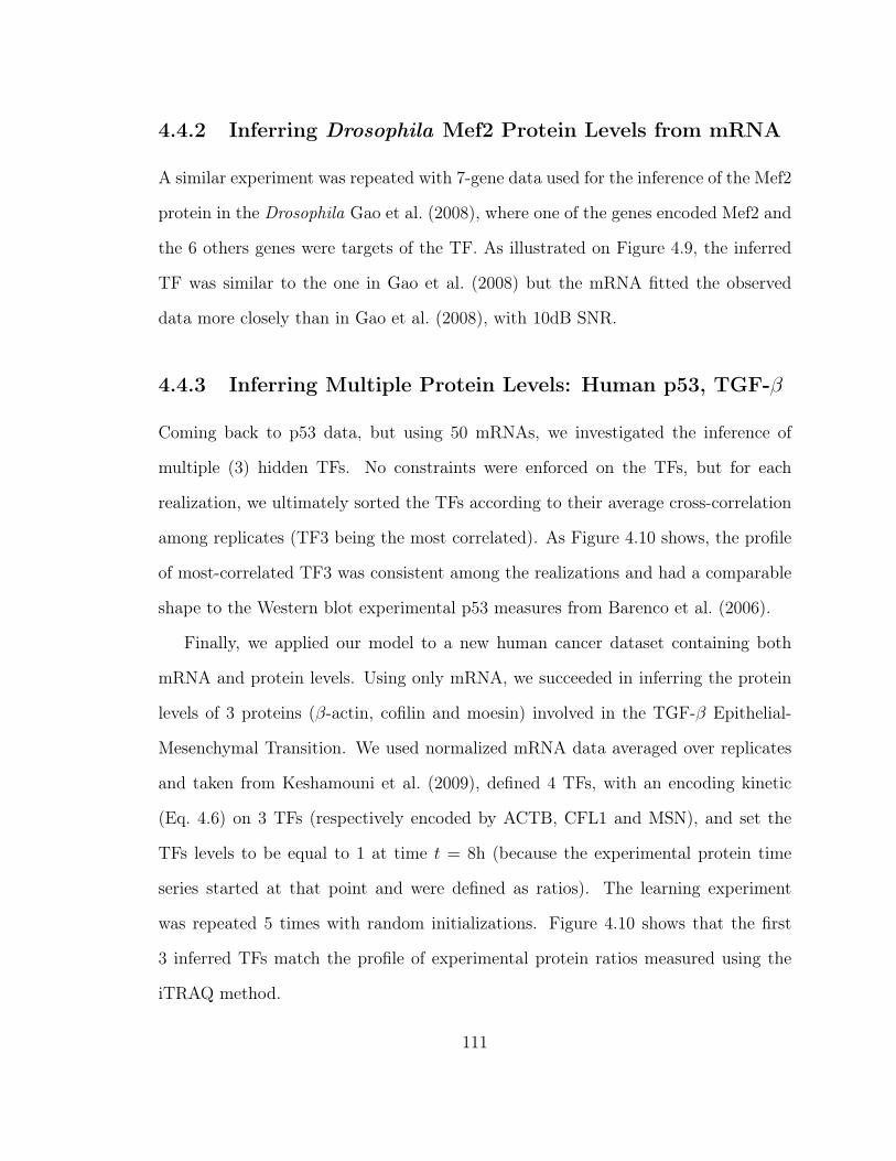
4.4.2 Inferring Drosophila Mef2 Protein Levels from mRNA

A similar experiment was repeated with 7-gene data used for the inference of the Mef2

protein in the Drosophila Gao et al. (2008), where one of the genes encoded Mef2 and

the 6 others genes were targets of the TF. As illustrated on Figure 4.9, the inferred

TF was similar to the one in Gao et al. (2008) but the mRNA fitted the observed

data more closely than in Gao et al. (2008), with 10dB SNR.

4.4.3 Inferring Multiple Protein Levels: Human p53, TGF-β

Coming back to p53 data, but using 50 mRNAs, we investigated the inference of

multiple (3) hidden TFs. No constraints were enforced on the TFs, but for each

realization, we ultimately sorted the TFs according to their average cross-correlation

among replicates (TF3 being the most correlated). As Figure 4.10 shows, the profile

of most-correlated TF3 was consistent among the realizations and had a comparable

shape to the Western blot experimental p53 measures from Barenco et al. (2006).

Finally, we applied our model to a new human cancer dataset containing both

mRNA and protein levels. Using only mRNA, we succeeded in inferring the protein

levels of 3 proteins (β-actin, cofilin and moesin) involved in the TGF-β Epithelial-

Mesenchymal Transition. We used normalized mRNA data averaged over replicates

and taken from Keshamouni et al. (2009), defined 4 TFs, with an encoding kinetic

(Eq. 4.6) on 3 TFs (respectively encoded by ACTB, CFL1 and MSN), and set the

TFs levels to be equal to 1 at time t = 8h (because the experimental protein time

series started at that point and were defined as ratios). The learning experiment

was repeated 5 times with random initializations. Figure 4.10 shows that the first

3 inferred TFs match the profile of experimental protein ratios measured using the

iTRAQ method.

111

4.5 Conclusions and Further Work

Using experimental validation, we demonstrated that our simple and fast gradient-

based state-space model algorithm can infer protein profiles from mRNA datasets,

and match experimental measures of protein concentration levels.

We have also shown that they can be applied to the problem of reverse-engineering

gene regulation networks from mRNA, by using hidden variables to model the noise

in mRNA data. Using predictive modeling, we were able to predict the direction

taken by gene expression levels on out-of-sample micro-arrays, confirming that our

dynamic model succeeded in capturing the influences of the gene regulatory network.

We are now planning on further evaluating our method for reverse-engineering

GRNs by directly modeling transcription factors and by replacing gene-gene inter-

actions by gene-TF and TF-gene interactions. In our factor graph notation, that

corresponds to replacing a model with dynamics on hidden variables Z and an iden-

tity observation function Y = h (Z) by a proper transcription function ∂yt

∂t= h (zt)

and a translation function ∂zt

∂t= f (yt). Our current work is inspired by the module-

networks SSM approaches described in (Hirose et al., 2008; Yamaguchi et al., 2007,

2010) and by the fully-fledged Dynamic Bayesian Network approaches in (Rangel

et al., 2004; Beal et al., 2005).

112

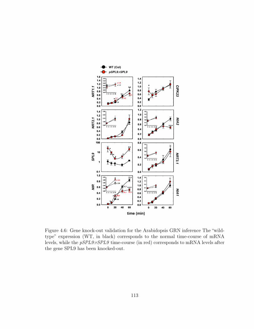
Figure 5

Figure 4.6: Gene knock-out validation for the Arabidopsis GRN inference The “wild-type” expression (WT, in black) corresponds to the normal time-course of mRNAlevels, while the pSPL9:rSPL9 time-course (in red) corresponds to mRNA levels afterthe gene SPL9 has been knocked-out.

113

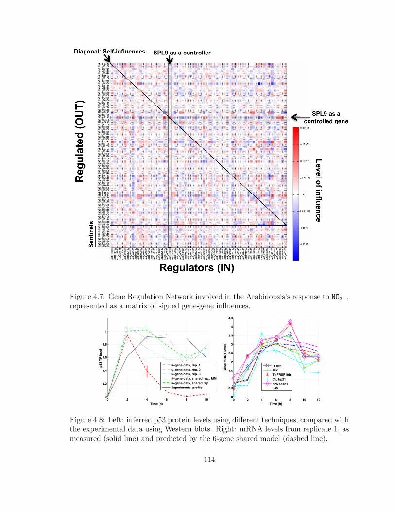
Figure 4

Figure 4.7: Gene Regulation Network involved in the Arabidopsis’s response to NO3−,represented as a matrix of signed gene-gene influences.

0 2 4 6 8 100

0.2

0.4

0.6

0.8

1

Time (h)

p53

TF le

vel

6−gene data, rep. 16−gene data, rep. 26−gene data, rep. 35−gene data, shared rep., MM6−gene data, shared rep.Experimental profile

Student Version of MATLAB

0 2 4 6 8 10 120

0.5

1

1.5

2

2.5

3

3.5

4

4.5

Gen

e m

RN

A le

vel

Time (h)

DDB2BIKTNFRSF10bCIp1/p21p26 sesn1p53


Figure 4.8: Left: inferred p53 protein levels using different techniques, compared withthe experimental data using Western blots. Right: mRNA levels from replicate 1, asmeasured (solid line) and predicted by the 6-gene shared model (dashed line).

114

1 2 3 4 5 6 7 8 9 10 11 12−0.5

0

0.5

1

1.5

2

2.5

3

3.5

4

4.5

5

Gen

e m

RN

A le

vel

Time (h)

FBgn0011656, Mef2FBgn0011286, Rya−r44FFBgn0022740, HLH54FFBgn0003870, ttkFBgn0026239, gukhFBgn0004885, tokFBgn0031037, HspB8


1 2 3 4 5 6 7 8 9 10 11−0.2

0

0.2

0.4

0.6

0.8

1

1.2

1.4

1.6

1.8

Mef

2 pr

otei

n TF

leve

l

Time (h)


Figure 4.9: Left: inferred Mef2 protein (10 different realizations). Right: mRNAlevels from replicate 1, as measured (solid line) and predicted by the model (dashedline).

0 2 4 6 8 10 0 2 4 6 8 10 0 2 4 6 8 10

TF1

TF2

TF3

Hid

den

prot

ein

TF le

vels

Time (h) for 3 replicates


0.5 1 2 4 8 16 24 72

TF1

TF2

TF3

TF4

Hid

den

prot

ein

TF le

vels

Time (h)

cofilin CFL1 (iTRAQ)

!−actin ACTB (iTRAQ)

moesin MSN (iTRAQ)


Figure 4.10: Left: inferred profiles of 3 latent variables, across 3 replicates, for the50-gene p53 dataset. For each of the 10 realizations, the latent factors were sortedby cross-correlation among replicates. TF3 has the strongest cross-correlation andresembles the p53 experimental profile. Right: inferrred profiles of 4 latent variablesfor the 70-gene TGF-β dataset. TF1, TF2 and TF3 are respectively encoded by theACTB, CFL1 and MSN genes and show very good fit to experimental iTRAQ ratios.

115

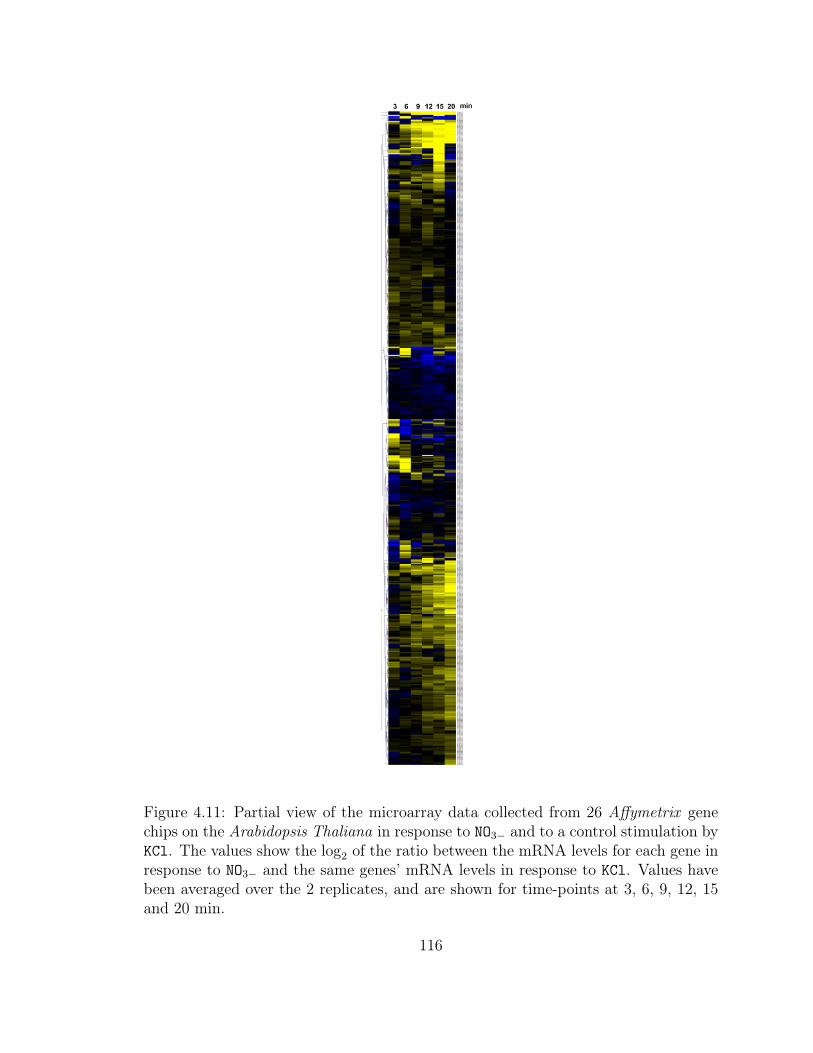
Figure 1

Figure 4.11: Partial view of the microarray data collected from 26 Affymetrix genechips on the Arabidopsis Thaliana in response to NO3− and to a control stimulation byKCl. The values show the log2 of the ratio between the mRNA levels for each gene inresponse to NO3− and the same genes’ mRNA levels in response to KCl. Values havebeen averaged over the 2 replicates, and are shown for time-points at 3, 6, 9, 12, 15and 20 min.

116

Chapter 5

Application to Topic Modeling of Time-Stamped

Documents

The Times They Are a-Changin’

Bob Dylan

This chapter introduces new applications for Dynamic Factor Graphs, consisting

in topic modeling, text classification and information retrieval. DFGs are tailored

here to sequences of time-stamped documents.

Based on the auto-encoder architecture, our nonlinear multi-layer model is trained

stage-wise to produce increasingly more compact representations of bags-of-words at

the document or paragraph level, thus performing a semantic analysis. It also incor-

porates simple temporal dynamics on the latent representations, to take advantage

of the inherent (hierarchical) structure of sequences of documents, and can simulta-

neously perform a supervised classification or regression on document labels, which

makes our approach unique. Learning this model is done by maximizing the joint like-

lihood of the encoding, decoding, dynamical and supervised modules, and is possible

using an approximate and gradient-based maximum-a-posteriori inference.

We demonstrate that by minimizing a weighted cross-entropy loss between his-

117

tograms of word occurrences and their reconstruction, we directly minimize the topic-

model perplexity, and show that our topic model obtains lower perplexity than the

Latent Dirichlet Allocation on the NIPS and State of the Union datasets. We illus-

trate how the dynamical constraints help the learning while enabling to visualize the

topic trajectory. Finally, we demonstrate superior information retrieval and classifica-

tion results on the Reuters collection, as well as an application to volatility forecasting

from financial news.

This work will be presented at the 2010 NIPS Deep Learning Workshop (Mirowski

et al., 2010c), and has been submitted for publication.

5.1 Information Retrieval, Topic Models and Auto-

Encoders

We propose in this article a new model for sequences of observations of discrete data,

specifically word counts in consecutive (or time-stamped) text documents, such as on-

line news, recurrent scientific publications or periodic political discourses. We build

upon the classical bag-of-words approach, which ignores the syntactic dependencies

between words, and focuses on the text semantics by looking at vocabulary distribu-

tions at the paragraph or document level. Our method can automatically discover

and exploit sequences of low-dimensional latent representations of such documents.

Unlike most latent variable or topic models, our latent representations can be simul-

taneously constrained both with simple temporal dependencies and with document

labels. One of our motivations is the sentiment analysis of streams of documents,

and has interesting business applications, such as ratings prediction. In this work,

we predict the volatility of a company’s stock, by capturing the opinion of investors

118

manifested in online news about that company.

5.1.1 Document Representation for Information Retrieval

Simple word counts-based techniques, such as the Term Frequency - Inverse Docu-

ment Frequency (TF-IDF) remain a standard method for information retrieval (IR)

tasks (for instance returning documents of the relevant category in response to a

query). TF-IDF can also be coupled with a classifier (such as an SVM with linear or

Gaussian kernels) to produce state-of-the-art text classifiers (Joachims, 1998; Debole

and Sebastiani, 2005). We thus show in Results section 5.3.3 how our low-dimensional

document representation measures up to TF-IDF or TF-IDF + SVM benchmarks on

information retrieval and text categorization tasks.

Plain TF-IDF relies on a high-dimensional representation of text (over all V words

in the vocabulary) and compact representations are preferable for index lookup be-

cause of storage and speed issues. A candidate for such low-dimensional representa-

tions is Latent Semantic Analysis (LSA) (Deerwester et al., 1990), which is based on

singular value decomposition (SVD). Alternatively, one can follow the dimensionality

reduction by independent components analysis (ICA), to obtain statistically inde-

pendent latent variables (Kolenda and Kai Hansen, 2000) (and, as we show in the

Results section, ICA-based LSA can achieves a better performance than simple LSA

in both information retrieval and text categorization tasks). Unfortunately, because

they perform lossy compression and are not trained discriminatively w.r.t. the task,

SVD and ICA achieve worse IR performance than the full TF-IDF.

Instead of linear dimensionality reduction, our approach is to build auto-encoders.

An auto-encoder is an architecture trained to provide with a latent representation

(encoding) of its input, thanks to a nonlinear encoder module and an associated

119

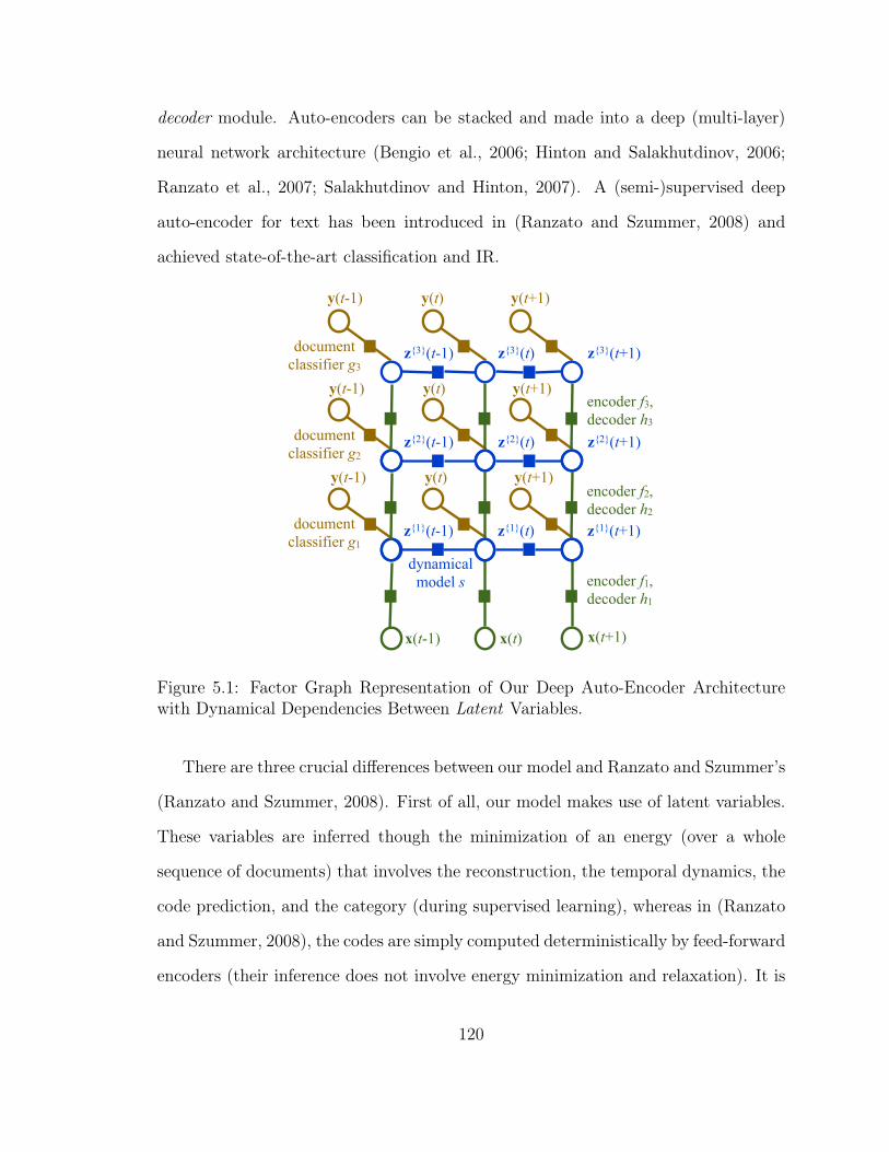
decoder module. Auto-encoders can be stacked and made into a deep (multi-layer)

neural network architecture (Bengio et al., 2006; Hinton and Salakhutdinov, 2006;

Ranzato et al., 2007; Salakhutdinov and Hinton, 2007). A (semi-)supervised deep

auto-encoder for text has been introduced in (Ranzato and Szummer, 2008) and

achieved state-of-the-art classification and IR.

z1(t-1) z1(t) z1(t+1)documentclassifier g1

dynamicalmodel s

x(t-1) x(t) x(t+1)


y(t-1) y(t) y(t+1)


encoder f3,decoder h3

y(t-1) y(t) y(t+1)

y(t-1) y(t) y(t+1)encoder f2,decoder h2

encoder f1,decoder h1

Figure 5.1: Factor Graph Representation of Our Deep Auto-Encoder Architecturewith Dynamical Dependencies Between Latent Variables.

There are three crucial differences between our model and Ranzato and Szummer’s

(Ranzato and Szummer, 2008). First of all, our model makes use of latent variables.

These variables are inferred though the minimization of an energy (over a whole

sequence of documents) that involves the reconstruction, the temporal dynamics, the

code prediction, and the category (during supervised learning), whereas in (Ranzato

and Szummer, 2008), the codes are simply computed deterministically by feed-forward

encoders (their inference does not involve energy minimization and relaxation). It is

120

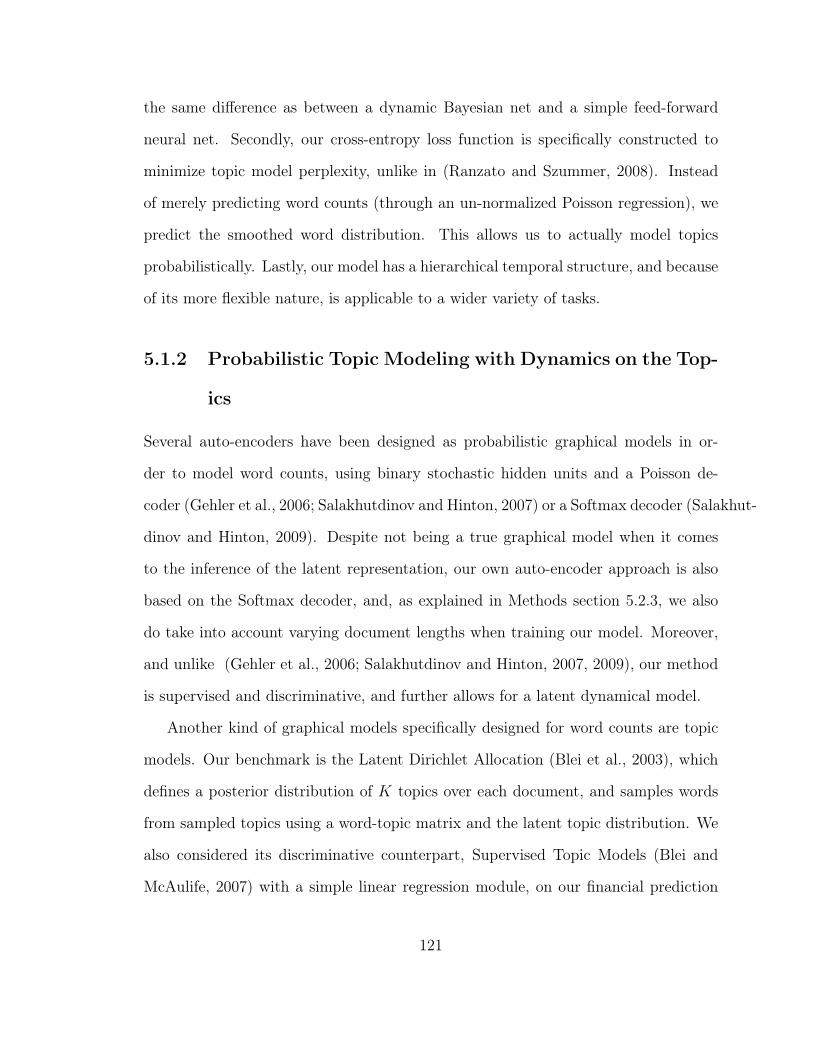
the same difference as between a dynamic Bayesian net and a simple feed-forward

neural net. Secondly, our cross-entropy loss function is specifically constructed to

minimize topic model perplexity, unlike in (Ranzato and Szummer, 2008). Instead

of merely predicting word counts (through an un-normalized Poisson regression), we

predict the smoothed word distribution. This allows us to actually model topics

probabilistically. Lastly, our model has a hierarchical temporal structure, and because

of its more flexible nature, is applicable to a wider variety of tasks.

5.1.2 Probabilistic Topic Modeling with Dynamics on the Top-

ics

Several auto-encoders have been designed as probabilistic graphical models in or-

der to model word counts, using binary stochastic hidden units and a Poisson de-

coder (Gehler et al., 2006; Salakhutdinov and Hinton, 2007) or a Softmax decoder (Salakhut-

dinov and Hinton, 2009). Despite not being a true graphical model when it comes

to the inference of the latent representation, our own auto-encoder approach is also

based on the Softmax decoder, and, as explained in Methods section 5.2.3, we also

do take into account varying document lengths when training our model. Moreover,

and unlike (Gehler et al., 2006; Salakhutdinov and Hinton, 2007, 2009), our method

is supervised and discriminative, and further allows for a latent dynamical model.

Another kind of graphical models specifically designed for word counts are topic

models. Our benchmark is the Latent Dirichlet Allocation (Blei et al., 2003), which

defines a posterior distribution of K topics over each document, and samples words

from sampled topics using a word-topic matrix and the latent topic distribution. We

also considered its discriminative counterpart, Supervised Topic Models (Blei and

McAulife, 2007) with a simple linear regression module, on our financial prediction

121

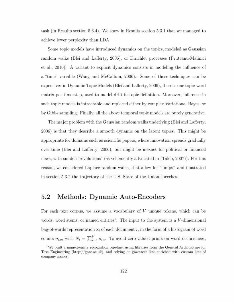
task (in Results section 5.3.4). We show in Results section 5.3.1 that we managed to

achieve lower perplexity than LDA.

Some topic models have introduced dynamics on the topics, modeled as Gaussian

random walks (Blei and Lafferty, 2006), or Dirichlet processes (Pruteanu-Malinici

et al., 2010). A variant to explicit dynamics consists in modeling the influence of

a “time” variable (Wang and McCallum, 2006). Some of those techniques can be

expensive: in Dynamic Topic Models (Blei and Lafferty, 2006), there is one topic-word

matrix per time step, used to model drift in topic definition. Moreover, inference in

such topic models is intractable and replaced either by complex Variational Bayes, or

by Gibbs sampling. Finally, all the above temporal topic models are purely generative.

The major problem with the Gaussian random walks underlying (Blei and Lafferty,

2006) is that they describe a smooth dynamic on the latent topics. This might be

appropriate for domains such as scientific papers, where innovation spreads gradually

over time (Blei and Lafferty, 2006), but might be inexact for political or financial

news, with sudden “revolutions” (as vehemently advocated in (Taleb, 2007)). For this

reason, we considered Laplace random walks, that allow for “jumps”, and illustrated

in section 5.3.2 the trajectory of the U.S. State of the Union speeches.

5.2 Methods: Dynamic Auto-Encoders

For each text corpus, we assume a vocabulary of V unique tokens, which can be

words, word stems, or named entities1. The input to the system is a V -dimensional

bag-of-words representation xi of each document i, in the form of a histogram of word

counts ni,v, with Ni =∑V

v=1 ni,v. To avoid zero-valued priors on word occurrences,

1We built a named-entity recognition pipeline, using libraries from the General Architecture forText Engineering (http://gate.ac.uk), and relying on gazetteer lists enriched with custom lists ofcompany names.

122

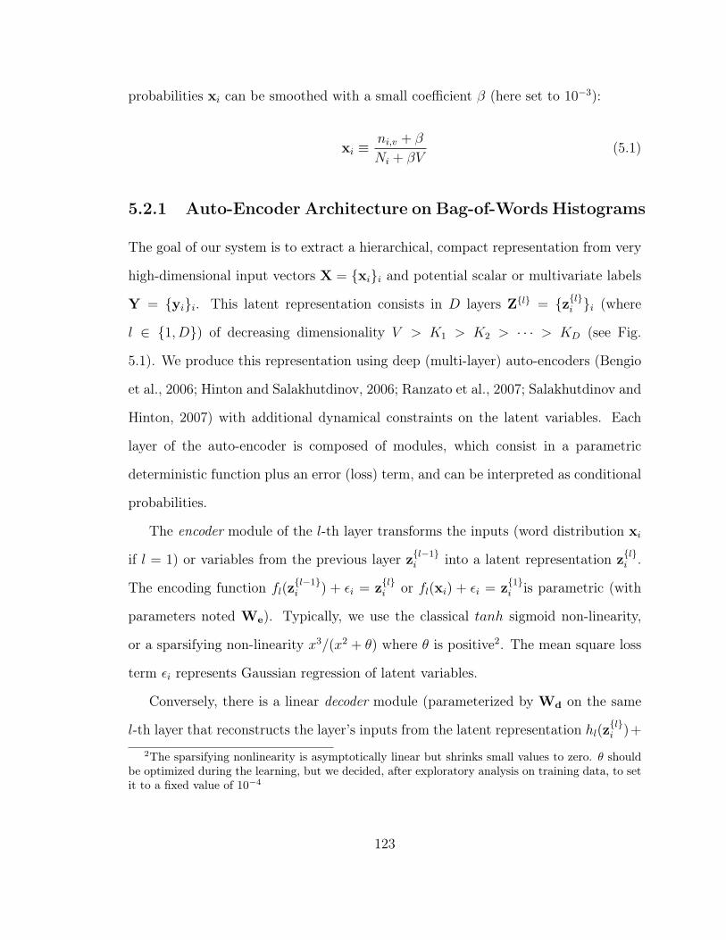
probabilities xi can be smoothed with a small coefficient β (here set to 10−3):

xi ≡ni,v + β

Ni + βV(5.1)

5.2.1 Auto-Encoder Architecture on Bag-of-Words Histograms

The goal of our system is to extract a hierarchical, compact representation from very

high-dimensional input vectors X = xii and potential scalar or multivariate labels

Y = yii. This latent representation consists in D layers Zl = zli i (where

l ∈ 1, D) of decreasing dimensionality V > K1 > K2 > · · · > KD (see Fig.

5.1). We produce this representation using deep (multi-layer) auto-encoders (Bengio

et al., 2006; Hinton and Salakhutdinov, 2006; Ranzato et al., 2007; Salakhutdinov and

Hinton, 2007) with additional dynamical constraints on the latent variables. Each

layer of the auto-encoder is composed of modules, which consist in a parametric

deterministic function plus an error (loss) term, and can be interpreted as conditional

probabilities.

The encoder module of the l-th layer transforms the inputs (word distribution xi

if l = 1) or variables from the previous layer zl−1i into a latent representation z

li .

The encoding function fl(zl−1i ) + εi = z

li or fl(xi) + εi = z

1i is parametric (with

parameters noted We). Typically, we use the classical tanh sigmoid non-linearity,

or a sparsifying non-linearity x3/(x2 + θ) where θ is positive2. The mean square loss

term εi represents Gaussian regression of latent variables.

Conversely, there is a linear decoder module (parameterized by Wd on the same

l-th layer that reconstructs the layer’s inputs from the latent representation hl(zli )+

2The sparsifying nonlinearity is asymptotically linear but shrinks small values to zero. θ shouldbe optimized during the learning, but we decided, after exploratory analysis on training data, to setit to a fixed value of 10−4

123

−

w

xwt log xw

t

h (zt;Wd)

f (xt;We)

xtzt

zt

zt

zt − zt 1

Id(zt−1)zt−1

yt−1 yt

xtxt−1

zt − zt 22

yt − yt 22

g (zt;Wc)

yt

αcLc,t

αeLe,t

Ld,t

Ls,t

Figure 5.2: Energy-based view of the first layer of the dynamic auto-encoder. Thereconstruction factor comprises a decoder module h with cross-entropy loss Ld,t w.r.t.word distribution xwt Vw=1, and an encoder module f with Gaussian loss Le,t, for atotal factor’s loss αeLe,t + Ld,t. The latent variables zt are averaged by time unitinto Zt′−1,Zt′ , . . . , and the latter follow Gaussian or Laplace random walk dynamicsdefined by the dynamical factor and associated loss αsLs,t′ (for simplicity, we assumedhere 1 document for time unit t′ and one for previous time unit t′ − 1). Thereis an optional supervised classification/regression module g (here with a Gaussianregression loss αcLc,t).

δi = zl−1i , with a Gaussian loss δi. Layer 1 is special, with a normal encoder but

with a Softmax decoder h1 and a cross-entropy loss term, as in (Salakhutdinov and

Hinton, 2009):

xvi =exp(Wdvz

1i )

∑v′ exp(Wdv′z

1i )

(5.2)

The dynamical module of the l-th layer corresponds to a simple random walk from a

document at time step t to next document at time step t+1: zlt+1 = z

lt +ηi. The error

124

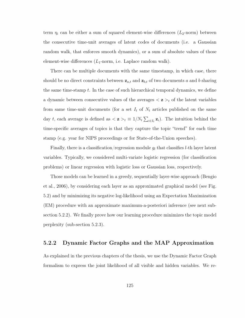
term ηi can be either a sum of squared element-wise differences (L2-norm) between

the consecutive time-unit averages of latent codes of documents (i.e. a Gaussian

random walk, that enforces smooth dynamics), or a sum of absolute values of those

element-wise differences (L1-norm, i.e. Laplace random walk).

There can be multiple documents with the same timestamp, in which case, there

should be no direct constraints between za,t and zb,t of two documents a and b sharing

the same time-stamp t. In the case of such hierarchical temporal dynamics, we define

a dynamic between consecutive values of the averages < z >t of the latent variables

from same time-unit documents (for a set It of Nt articles published on the same

day t, each average is defined as < z >t ≡ 1/Nt

∑i∈It zi). The intuition behind the

time-specific averages of topics is that they capture the topic “trend” for each time

stamp (e.g. year for NIPS proceedings or for State-of-the-Union speeches).

Finally, there is a classification/regression module gl that classifies l-th layer latent

variables. Typically, we considered multi-variate logistic regression (for classification

problems) or linear regression with logistic loss or Gaussian loss, respectively.

Those models can be learned in a greedy, sequentially layer-wise approach (Bengio

et al., 2006), by considering each layer as an approximated graphical model (see Fig.

5.2) and by minimizing its negative log-likelihood using an Expectation Maximization

(EM) procedure with an approximate maximum-a-posteriori inference (see next sub-

section 5.2.2). We finally prove how our learning procedure minimizes the topic model

perplexity (sub-section 5.2.3).

5.2.2 Dynamic Factor Graphs and the MAP Approximation

As explained in the previous chapters of the thesis, we use the Dynamic Factor Graph

formalism to express the joint likelihood of all visible and hidden variables. We re-

125

trieve through a MAP inference the most likely sequence of hidden topics Z (minimiza-

tion of an unnormalized negative log-likelihood). Our gradient-based EM algorithm

is a coordinate descent on the log-likelihood over the sequence:

L(X,Y; W) = minZ

Ld(X,Z; Wd) +

αcLc(Z,Y; Wc) +

αeLe(X,Z; We) +

αsLs(Z)

(5.3)

Each iterative inference (E-step) and learning (M-step) consists in a full relaxation

w.r.t. latent variables or parameters, like in the original EM algorithm. We use simple

gradient descent to minimize negative log-likelihood loss w.r.t. latent variables, and

conjugate gradient with line search to mimize L w.r.t. parameters. Because each

relaxation is until convergence and done separately, everything else being fixed, the

various hyperparameters for learning the modules can be tuned independently, and

the only subtlety is in the choice of the weights αc, αe and αs. The α∗ coefficients

control the relative importance of the encoder, decoder, dynamics and supervised

modules in the total energy, and they can be chosen by cross-validation.

We add an additional Laplace prior on the weights and latent variables (using

L1-norm regularization, and multiplying learning rates by λw = λz = 10−4). Finally,

we normalize the decoder to unit column weights as in the sparse decomposition (Ol-

shausen and Field, 1997). Because we initialize the latent variable by first propagating

the inputs of the layer through the encoder, then doing a relaxation, the relaxation

always gives the same latent variables for given parameters, inputs and labels.

As a variation on a theme, we can directly encode xi using the encoders f1, f2, . . . , fD,

like in (Ranzato and Szummer, 2008), in order to perform fast inference (e.g. for in-

formation retrieval or for prediction, as we did on experiments in sections 5.3.3 or

126

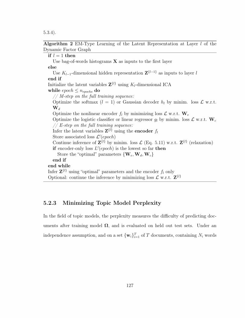
5.3.4).

Algorithm 2 EM-Type Learning of the Latent Representation at Layer l of theDynamic Factor Graphif l = 1 then

Use bag-of-words histograms X as inputs to the first layerelse

Use Kl−1-dimensional hidden representation Zl−1 as inputs to layer lend ifInitialize the latent variables Zl using Kl-dimensional ICAwhile epoch ≤ nepochs do// M-step on the full training sequence:Optimize the softmax (l = 1) or Gaussian decoder hl by minim. loss L w.r.t.Wd

Optimize the nonlinear encoder fl by minimizing loss L w.r.t. We

Optimize the logistic classifier or linear regressor gl by minim. loss L w.r.t. Wc

// E-step on the full training sequence:Infer the latent variables Zl using the encoder flStore associated loss L′(epoch)Continue inference of Zl by minim. loss L (Eq. 5.11) w.r.t. Zl (relaxation)if encoder-only loss L′(epoch) is the lowest so far then

Store the “optimal” parameters We,Wd,Wcend if

end whileInfer Zl using “optimal” parameters and the encoder fl onlyOptional: continue the inference by minimizing loss L w.r.t. Zl

5.2.3 Minimizing Topic Model Perplexity

In the field of topic models, the perplexity measures the difficulty of predicting doc-

uments after training model Ω, and is evaluated on held out test sets. Under an

independence assumption, and on a set wiTi=1 of T documents, containing Ni words

127

each, perplexity is defined in (Blei et al., 2003) as the exponential of the cross-entropy:

P ≡ p(wiTi=1|Ω

)− 1PTi=1

Ni (5.4)

= exp

(−∑T

i=1 log p (wi|Ω)∑Ti=1Ni

)(5.5)

In most topic models, each document i is associated with a latent representation θi

(e.g. the multinomial posterior distribution over topics in LDA), and one assumes the

document to be a bag of Ni conditionally independent words wi = wi,nNin=1. Hence,

the marginal distribution of wi is:

p (wi|Ω) =

∫

θi

p (θi|Ω)

(Ni∏

n=1

p(wi,n|θi,Ω)

)dθi (5.6)

≈Ni∏

n=1

p(wi,n|θi,Ω) (5.7)

Estimating the likelihood of a document given a topic model is intractable even for

small number of topics, documents and vocabulary size, although approximate tech-

niques based on particle filtering were recently suggested in (Buntine, 2009). Here,

we use the standard approximation made by LDA, which is that the topic assignment

distribution θi is inferred for each document d from observed word occurrences using

variational inference (Blei et al., 2003) or Gibbs sampling (Griffiths and Steyvers,

2004). In our maximum-a-posteriori approach, we replace the full distribution over θi

by a delta distribution with a mode at θi that maximizes the likelihood. We rewrite

128

equation (5.6):

log p(wi|θi,Ω

)=

Ni∑

n=1

log p(wi,n|θi,Ω) (5.8)

= Ni

V∑

v=1

ni,vNi

log p(v|θi,Ω) (5.9)

By defining the empirical conditional distribution of words in document d as pi(v) ≡ni,v

Ni, which we substitute in (5.8), and by noting the model conditional distribution as

qi(v) ≡ p(v|θi.Ω), equation (5.8) become proportional to the cross-entropy between

the empirical and the model conditional distributions over words for document i:

H (pi(v), qi(v)) = −∑v pi(v) log qi(v). Given this derivation and MAP approxima-

tion, the perplexity of our topic model can be expressed in terms of a weighted sum

of cross-entropies (the weights are proportional to the documents’ lengths):

P ≈ P = exp

(1∑Ti=1Ni

T∑

i=1

NiH(pi, qi)

)(5.10)

Minimizing LDA perplexity (5.4) is equivalent to minimizing the negative log-likelihood

of the model probabilities of words in all documents, i.e. to a maximum likelihood so-

lution. This is what we do in our approximate maximum-a-posteriori (MAP) solution,

by minimizing a weighted cross-entropy loss (5.11) with respect to both the model

parameters Ω and the latent representations θiTi=1. Using an unnormalized latent

document representation zi (instead of LDA’s simplex θi), and in lieu of model distri-

bution qi, our model reconstructs a V -dimensional output vector xi of positive values

summing to 1 through the sequence of decoding functions (we write it xi = h(zi)).

However, instead of integrating over the latent variables as in (5.6), we minimize the

reconstruction loss (5.11) over the hidden representation. For a document i, the cross-

129

entropy −∑v xi,v log xi,v is measured between the actually observed distribution xi,

and the predicted distribution xi.

Ld(piTi=1; Ω

)≡ min

qii

(T∑

i=1

NiH(pi, qi)

)(5.11)

= minxi

(−

T∑

i=1

xTi log xi

)(5.12)

5.3 Results Obtained with Dynamic Auto-Encoders

5.3.1 Perplexity of Unsupervised Dynamic Auto-Encoders

In order to evaluate the quality of Dynamic Auto-Encoders as topic models, we per-

formed a comparison of DAE vs. Latent Dirichlet Allocation. More specifically, for a

100-30-10-2 DAE architecture, we compared the perplexity of 100-topic LDA vs. the

perplexity of the 1st layer of the DAE, then the perplexities of 30-topic LDA vs. the

2nd DAE layer, and so on for 10-topic and 2-topic LDA.

The dataset, consisting in 2483 NIPS articles published from 1987 to 2003, was

separated into a training set (2286 articles until 2002) and a test set (197 articles from

2003). We kept the top V = 2000 words with the highest TF-IDF score. 100-, 30-, 10-

and 2-topic LDA “encodings” (Blei et al., 2003) were performed using Gibbs sampling

inference3 (Griffiths and Steyvers, 2004). Our 100-30-10 DAE with encoding weight

αe = 0 achieved lower perplexity4 than LDA on the first two layers (see Table 5.1).

We also empirically compared L1 or L2 dynamical penalties vs. no dynamics (αs = 0).3Using Xuan-Hieu Phan’s GibbsLDA++ package, available at http://gibbslda.sourceforge.net/,

we trained Gibbs-sampled sLDA for 2000 iterations, with standard and recommended priors α =50/M and β = 20/V

4Note that we did not evaluate the perplexity of unigram representations of text, which havebeen shown in (Blei et al., 2003) to perform much worse than LDA.

130

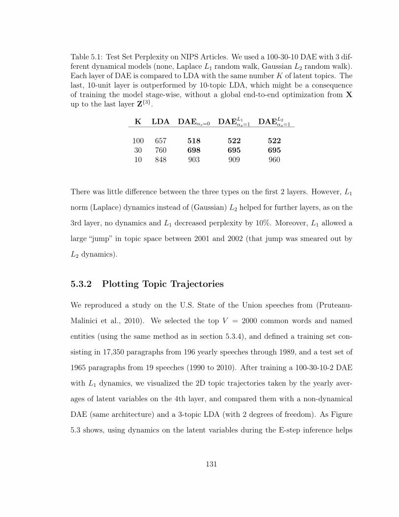
Table 5.1: Test Set Perplexity on NIPS Articles. We used a 100-30-10 DAE with 3 dif-ferent dynamical models (none, Laplace L1 random walk, Gaussian L2 random walk).Each layer of DAE is compared to LDA with the same numberK of latent topics. Thelast, 10-unit layer is outperformed by 10-topic LDA, which might be a consequenceof training the model stage-wise, without a global end-to-end optimization from Xup to the last layer Z3.

K LDA DAEαs=0 DAEL1αs=1 DAEL2

αs=1

100 657 518 522 52230 760 698 695 69510 848 903 909 960

There was little difference between the three types on the first 2 layers. However, L1

norm (Laplace) dynamics instead of (Gaussian) L2 helped for further layers, as on the

3rd layer, no dynamics and L1 decreased perplexity by 10%. Moreover, L1 allowed a

large “jump” in topic space between 2001 and 2002 (that jump was smeared out by

L2 dynamics).

5.3.2 Plotting Topic Trajectories

We reproduced a study on the U.S. State of the Union speeches from (Pruteanu-

Malinici et al., 2010). We selected the top V = 2000 common words and named

entities (using the same method as in section 5.3.4), and defined a training set con-

sisting in 17,350 paragraphs from 196 yearly speeches through 1989, and a test set of

1965 paragraphs from 19 speeches (1990 to 2010). After training a 100-30-10-2 DAE

with L1 dynamics, we visualized the 2D topic trajectories taken by the yearly aver-

ages of latent variables on the 4th layer, and compared them with a non-dynamical

DAE (same architecture) and a 3-topic LDA (with 2 degrees of freedom). As Figure

5.3 shows, using dynamics on the latent variables during the E-step inference helps

131

to produce a latent representation that can be useful when we expect a dynamical

structure in the data.

The latter 2D latent representation provided us with a historical interpretation. It

appeared that the five strongest discontinuities in the L1 norm between 4-th hidden

topics were, in that order: Harry Truman (1946), Ronald Reagan (1982, inaugural),

Andrew Jackson (1829, inaugural), Woodrow Wilson (1913, inaugural) and Franklin

Roosevelt (1934, inaugural), and on the test data, George W Bush (2001, inaugu-

ral), William Clinton (1996) and Barack Obama (2009, inaugural), which seemed to

confirm historical intuitions.

Hierarchical trajectory over time of latent topics (3−topic LDA)

1790GeorgeWashington

1797JohnAdams

1801ThomasJefferson

1809JamesMadison

1817JamesMonroe

1825JohnQuincyAdams

1829AndrewJackson

1837MartinvanBuren1841JohnTyler1845JamesPolk

1849ZacharyTaylor1850MillardFillmore

1853FranklinPierce

1857JamesBuchanan

1861AbrahamLincoln

1865AndrewJohnson

1869UlyssesSGrant1877RutherfordBHayes

1881ChesterAArthur1885GroverCleveland

1889BenjaminHarrison1897WilliamMcKinley

1901TheodoreRoosevelt

1909WilliamHTaft

1913WoodrowWilson1921WarrenHarding

1923CalvinCoolidge1929HerbertHoover

1934FranklinDRoosevelt

1946HarrySTruman

1953DwightDEisenhower

1953HarrySTruman

1954DwightDEisenhower

1961JohnFKennedy

1964LyndonBJohnson1970RichardNixon

1975GeraldRFord

1978JimmyCarter

1982RonaldReagan

UNITED STATES power GOVERNMENT citizen subject country law treaty government act

peo

ple

natio

n wa

r wor

ld p

eace

am

erica

n po

licy

natio

nal c

ontin

ue c

ount

ry


−0.2 −0.15 −0.1 −0.05 0 0.05 0.1 0.15 0.2 0.25−0.6

−0.4

−0.2

0

0.2

0.4

0.6

0.8

1

1.2Hierarchical trajectory over time of latent topics

1790GeorgeWashington1797JohnAdams1801ThomasJefferson 1809JamesMadison

1817JamesMonroe

1825JohnQuincyAdams

1829AndrewJackson1837MartinvanBuren1841JohnTyler1845JamesPolk1849ZacharyTaylor

1850MillardFillmore1853FranklinPierce1857JamesBuchanan

1861AbrahamLincoln1865AndrewJohnson

1869UlyssesSGrant1877RutherfordBHayes 1881ChesterAArthur1885GroverCleveland

1889BenjaminHarrison1897WilliamMcKinley 1901TheodoreRoosevelt

1909WilliamHTaft

1913WoodrowWilson

1921WarrenHarding1923CalvinCoolidge

1929HerbertHoover

1934FranklinDRoosevelt1946HarrySTruman

1953DwightDEisenhower1953HarrySTruman1954DwightDEisenhower

1961JohnFKennedy1964LyndonBJohnson

1970RichardNixon

1975GeraldRFord

1978JimmyCarter

1982RonaldReagan

preserve mutual understanding strengthen independence vs. expenditure receipt TREASURY fiscal sum

toni

ght c

halle

nge

ahea

d co

mm

itmen

t AM

ERIC

A w

oman

dre

am

vs. d

eem

gov

ernm

ent p

rope

r unj

urio

us m

anne

r obj

ect r

egar

d


−0.4 −0.2 0 0.2 0.4 0.6 0.8 1−1.2

−1

−0.8

−0.6

−0.4

−0.2

0

0.2Hierarchical trajectory over time of latent topics

1790GeorgeWashington

1797JohnAdams

1801ThomasJefferson

1809JamesMadison

1817JamesMonroe

1825JohnQuincyAdams1829AndrewJackson

1837MartinvanBuren

1841JohnTyler

1845JamesPolk

1849ZacharyTaylor1850MillardFillmore

1853FranklinPierce

1857JamesBuchanan

1861AbrahamLincoln

1865AndrewJohnson

1869UlyssesSGrant

1877RutherfordBHayes

1881ChesterAArthur

1885GroverCleveland1889BenjaminHarrison

1897WilliamMcKinley

1901TheodoreRoosevelt

1909WilliamHTaft

1913WoodrowWilson

1921WarrenHarding1923CalvinCoolidge

1929HerbertHoover

1934FranklinDRoosevelt1946HarrySTruman

1953DwightDEisenhower1953HarrySTruman

1954DwightDEisenhower1961JohnFKennedy

1964LyndonBJohnson1970RichardNixon

1975GeraldRFord

1978JimmyCarter

1982RonaldReagan

expenditure fiscal receipt estimate TREASURY vs. preserve region regard independence standard

peop

le e

ffici

ency

wor

ld c

ombi

ne d

olla

r vs

. tre

aty

conv

entio

n ar

bitra

tion

com

mis

sion

er G

REA

T BRIT

AIN


Figure 5.3: 2D “Trajectories” of State-of-the-Union Addresses. Left: We visualizethe 4th layer yearly topic averages (over paragraphs) of 196 addresses, produced bya 100-30-10-2 DAE, with dynamical weight αs = 1. On each axis, “vs.” opposes thewords at the two extremes of that axis. Latent variables were inferred per paragraphand averaged by year. Top right: same figure for a DAE without dynamics (αs = 0).Bottom right: same figure for a 3-topic LDA (2 degrees of freedom).

132

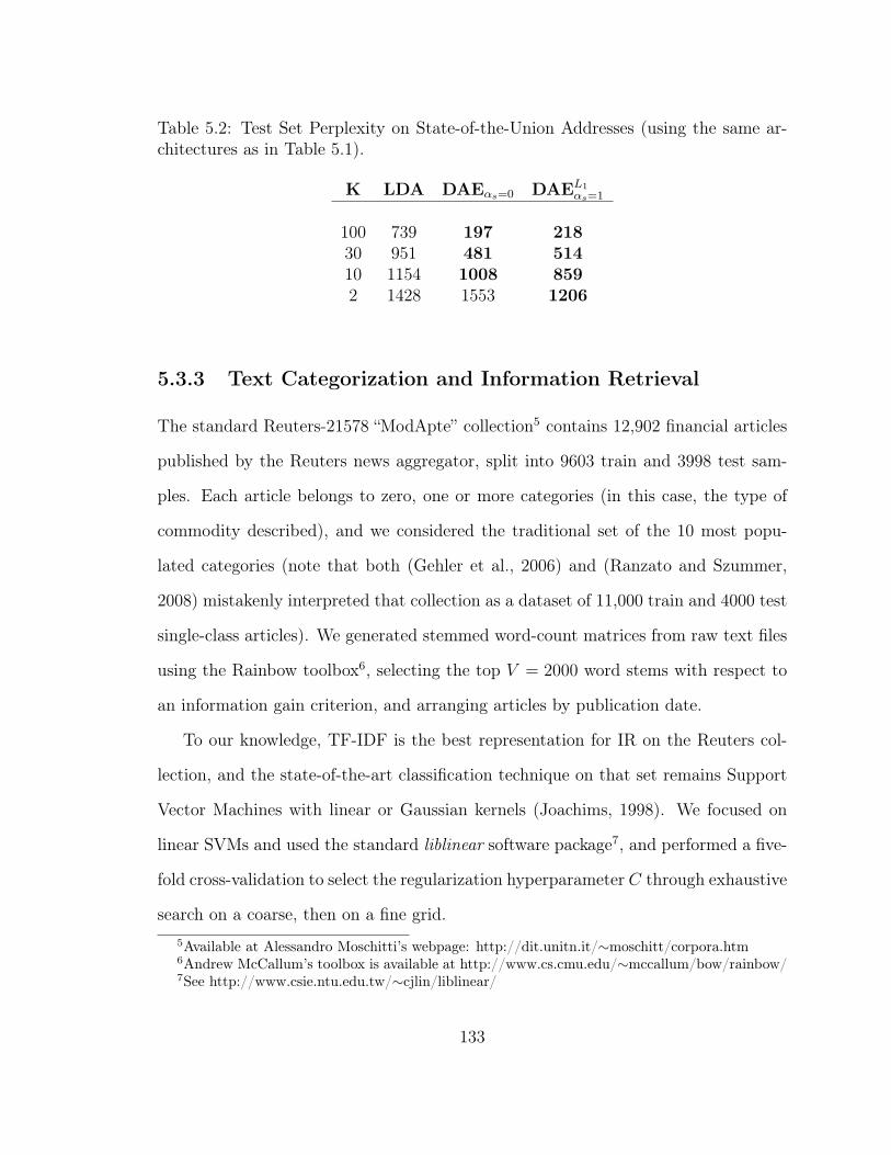
Table 5.2: Test Set Perplexity on State-of-the-Union Addresses (using the same ar-chitectures as in Table 5.1).

K LDA DAEαs=0 DAEL1αs=1

100 739 197 21830 951 481 51410 1154 1008 8592 1428 1553 1206

5.3.3 Text Categorization and Information Retrieval

The standard Reuters-21578 “ModApte” collection5 contains 12,902 financial articles

published by the Reuters news aggregator, split into 9603 train and 3998 test sam-

ples. Each article belongs to zero, one or more categories (in this case, the type of

commodity described), and we considered the traditional set of the 10 most popu-

lated categories (note that both (Gehler et al., 2006) and (Ranzato and Szummer,

2008) mistakenly interpreted that collection as a dataset of 11,000 train and 4000 test

single-class articles). We generated stemmed word-count matrices from raw text files

using the Rainbow toolbox6, selecting the top V = 2000 word stems with respect to

an information gain criterion, and arranging articles by publication date.

To our knowledge, TF-IDF is the best representation for IR on the Reuters col-

lection, and the state-of-the-art classification technique on that set remains Support

Vector Machines with linear or Gaussian kernels (Joachims, 1998). We focused on

linear SVMs and used the standard liblinear software package7, and performed a five-

fold cross-validation to select the regularization hyperparameter C through exhaustive

search on a coarse, then on a fine grid.5Available at Alessandro Moschitti’s webpage: http://dit.unitn.it/∼moschitt/corpora.htm6Andrew McCallum’s toolbox is available at http://www.cs.cmu.edu/∼mccallum/bow/rainbow/7See http://www.csie.ntu.edu.tw/∼cjlin/liblinear/

133

We compared our 100-30-10-2 DAE with a single-hidden-layer Multi-Layer Per-

ceptron encoder to TF-IDF, TF-IDF+ICA (Kolenda and Kai Hansen, 2000), TF-

IDF+SVD (Deerwester et al., 1990), LDA (Blei et al., 2003; Griffiths and Steyvers,

2004), and auto-encoders (Ranzato and Szummer, 2008). The Area Under the Precision-

Recall (AUPR) curve for information retrieval (interpolated as in (Davis and Goad-

rich, 2006)) by TF-IDF was 0.51, and 0.54 using 10-dimensional LDA (which was by

far the best among unsupervised techniques). After optimizing the inference weights

on the training data (αe = αc = 10 and αs = 1), our DAE vastly outperformed

TF-IDF and unsupervised techniques in terms of AUPR (see Table 5.3). For the

multi-class classification task, we computed multi-class precision, recall and F1 scores

using micro and macro-averaging (Joachims, 1998; Debole and Sebastiani, 2005). Us-

ing an SVM with linear kernel trained on the latent variables, we matched full TF-IDF

(F1,µ = 0.91, F1,M = 0.83)8 and outperformed TF-IDF+ICA (see Table 5.4).

Auto-encoders (Ranzato and Szummer, 2008) with the same architecture as DAE

performed slightly better than DAE in terms of AUPR for IR, which might be at-

tributed to the fact that they have no relaxation step on the latent variables during

learning, only direct inference, which might help to better train the encoder. We can

nevertheless claim that DAEs are close to the state of the art for information retrieval

and text classification.

5.3.4 Prediction of Stock Market Volatility from Online News

There is some evidence in recent history that financial markets (over)react to public

information. In a simpler setting, one can restrict this observation to company-

specific news and associated stock movements, quantified with volatility σ2. The

problems of stock price movement or volatility forecasting from financial news have8TF-IDF with Gaussian SVR achieved (F1,µ = 0.92, F1,M = 0.84).

134

Table 5.3: Test Set Area Under the Prediction-Recall for Information Retrieval onReuters-21578 Articles. We used a 100-30-10-2 DAE with 2 different dynamical mod-els (none vs. Laplace L1 random walk). Each layer of DAE is compared to LDA,TFIDF+ICA or TFIDF+SVD with the same numberK of latent topics (TFIDF+ICAperformed the best). We outperformed full TFIDF (0.51) and all unsupervised tech-niques. We also compared our architecture to auto-encoders in (Ranzato and Szum-mer, 2008) with a similar 100-30-10-2 architecture.

K LDA DAEαc=10αs=0 DAEαc=10

L1,αs=1 DAEαc=100αs=0 DAEαc=100

L1,αs=1 R&S

100 0.42 0.86 0.86 0.90 0.89 0.8730 0.49 0.85 0.81 0.62 0.63 0.9310 0.54 0.86 0.80 0.81 0.78 0.892 0.25 0.73 0.78 0.71 0.75 0.70

Table 5.4: Test Set Macro/Micro-Averaged F1 Scores Using Linear SVM on Reuters-21578 Articles. We used the same architectures as in Table 5.3.

K ICA DAEαc=10αs=0 DAEαc=10

L1,αs=1 DAEαc=100αs=0 DAEαc=100

L1,αs=1 R&S

100 0,90, 0.81 0.91, 0.84 0.91, 0.84 0.92, 0.86 0.92, 0.85 0.92, 0.8530 0.86, 0.70 0,91, 0.85 0.91, 0.83 0.92, 0.86 0.92, 0.85 0.92, 0.8510 0.73, 0.40 0.91, 0.84 0.91, 0.84 0.92, 0.86 0.92, 0.85 0.92, 0.842 0.53, 0.09 0.81, 0.52 0.85, 0.63 0.83, 0.54 0.83, 0.51 0.75, 0.19

been formulated as supervised text categorization problems, and addressed in an

intra-day setting, respectively in (Gidofalvi and Elkan, 2003) and in (Robertson et al.,

2007). In the latter, it was proved that the arrival of some “shock” news about

an asset j impacted its volatility (by switching to a “high-volatility” mode) for a

duration of at least 15 min. In this article, we tried to solve a slightly more difficult

problem than in (Robertson et al., 2007), by considering the volatility σ2j,t estimated

from daily stock prices9 of a company j. We normalized volatility dividing it by the9Stock market data were acquired at http://finance.yahoo.com. Volatility was estimated from

daily open, close, high and low prices (Yang and Zhang, 2000).

135

median volatility across all companies j on that same day, then taking its logarithm:

yj,t = log σ2j,t − log σ2

t . Using the Bloomberg Professional service, we collected over

90,000 articles, published between January 1 and December 31, 2008, on 30 companies

that were components of the Dow Jones index on June 30, 2008. We extracted each

document’s time stamp and matched it to the log-volatility measure yj,t at the earliest

following market closing time. Common words and named entities were extracted, and

numbers (dollar amounts, percentages) were binned. In order to make the problem

challenging, we split the dataset into 51,362 test articles (after July 1, 2008, in a crisis

market) and 38,968 training articles (up to June 30, 2008, corresponding to a more

optimistic market).

Our benchmark was linear regression on the 2000-word TF-IDF representation,

which achieved R2 = 0.267. Support Vector Regression with Gaussian kernels10 (and

a Gaussian “spread" parameter equal to γ = 1) achieved a higher score of R2 = 0.285.

Note that kernel methods are expensive on this large Bloomberg dataset with 51k

training examples. sLDA 11 (Blei and Lafferty, 2006) performed surprisingly poorly,

with R2 < 0.1, for 100, 30, 10 or 2 topics.

As we report in Table 5.5, our DAE with a 100-30-10-2 architecture, L1 dynamics,

tanh encoders f and linear decoders g achieves, at each hidden layer, a higher coeffi-

cient of determination R2 on the test set than linear encodings (K-dimensional ICA

on TF-IDF) or probabilistic topic models (K-topic LDA). We observe that the latent

representation on the 3rd and 4th layer of our DAE architecture also performs better

than the full high-dimensional sparse representation (TF-IDF). DAE were however

outperformed by the auto-encoders from (Ranzato and Szummer, 2008), for similar10We used the liblinear SVM library, available at: http://www.csie.ntu.edu.tw/ cjlin/libsvm/11Using Jonathan Chang’s LDA package available at http://cran.r-project.org/web/packages/lda,

we trained Gibbs-sampled sLDA with 100 M steps and 20 E steps, with priors α = 50/M andβ = 20/V

136

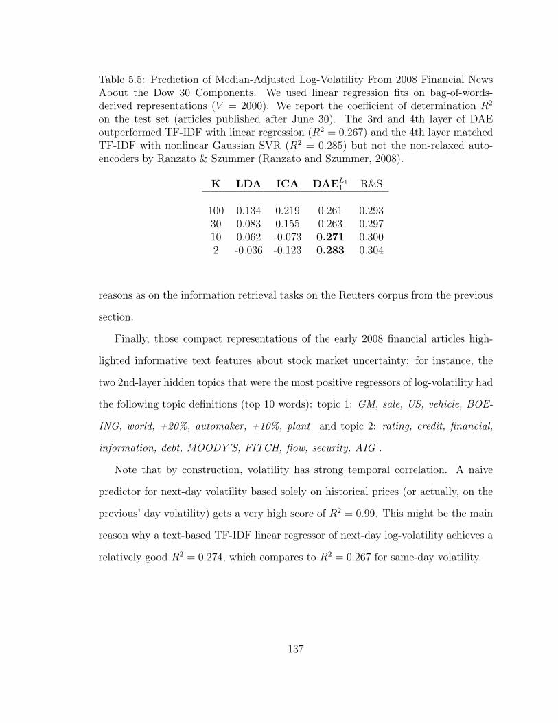
Table 5.5: Prediction of Median-Adjusted Log-Volatility From 2008 Financial NewsAbout the Dow 30 Components. We used linear regression fits on bag-of-words-derived representations (V = 2000). We report the coefficient of determination R2

on the test set (articles published after June 30). The 3rd and 4th layer of DAEoutperformed TF-IDF with linear regression (R2 = 0.267) and the 4th layer matchedTF-IDF with nonlinear Gaussian SVR (R2 = 0.285) but not the non-relaxed auto-encoders by Ranzato & Szummer (Ranzato and Szummer, 2008).

K LDA ICA DAEL11 R&S

100 0.134 0.219 0.261 0.29330 0.083 0.155 0.263 0.29710 0.062 -0.073 0.271 0.3002 -0.036 -0.123 0.283 0.304

reasons as on the information retrieval tasks on the Reuters corpus from the previous

section.

Finally, those compact representations of the early 2008 financial articles high-

lighted informative text features about stock market uncertainty: for instance, the

two 2nd-layer hidden topics that were the most positive regressors of log-volatility had

the following topic definitions (top 10 words): topic 1: GM, sale, US, vehicle, BOE-

ING, world, +20%, automaker, +10%, plant and topic 2: rating, credit, financial,

information, debt, MOODY’S, FITCH, flow, security, AIG .

Note that by construction, volatility has strong temporal correlation. A naive

predictor for next-day volatility based solely on historical prices (or actually, on the

previous’ day volatility) gets a very high score of R2 = 0.99. This might be the main

reason why a text-based TF-IDF linear regressor of next-day log-volatility achieves a

relatively good R2 = 0.274, which compares to R2 = 0.267 for same-day volatility.

137

5.4 Conclusions and Futher Work

We have introduced a new method for information retrieval, text categorization and

topic modeling, that can be trained in a both purely generative and discriminative

ways. It can give word probabilities per document, like in a topic model, and incorpo-

rates temporal dynamics on the topics. Moreover, learning and inference in our model

is simple, as it relies on an approximate MAP inference and a greedy approach for

multi-layer auto-encoders. This results in a few hours of learning time on moderately

large text corpora, using unoptimized Matlab code. Our initial results on standard

text collections are very promising. As further avenues of work, we are planning on

designing better (nonlinear) encoder modules, and in optimizing the gradient-based

algorithms for training individual components of the DAE, in order to speed-up the

method for very large datasets.

5.4.1 Application to Epileptic Seizure Prediction from EEG

I am also planning on applying Dynamic Auto-Encoders to our patent-pending (Mirowski

et al., 2009b) seizure prediction methodology. The latter consists in classifying pat-

terns xt of bi-variate EEG synchronization features into two types: pre-ictal (i.e. a few

minutes before a seizure) and interictal (far from seizure). The motivation behind

our work is that, despite the current lack of a complete neurological understand-

ing of the pre-ictal brain state, researchers increasingly hypothesize that brainwave

synchronization patterns might differentiate interictal, preictal and ictal (seizure)

states (Le Van Quyen et al., 2003). The meaures that we use for synchronization

are bivariate (between any two electrodes of multi-channel EEG), and can consist in

such features as cross-correlation, nonlinear interdependence (Arnhold et al., 1999)

138

or Wavelet analysis-based phase-locking synchony (Le Van Quyen et al., 2001). In

our previous published work (Mirowski et al., 2008, 2009a), we showed that by train-

ing patient-specific convolutional network classifiers, we can successfully predict all

seizures without false positives on the test set, in 15 patients out of 21, using a publicly

available EEG database12, and thus obtaining state-of-the-art performance on that

data, outperforming previous studies (Aschenbrenner-Scheibe et al., 2003; Maiwald

et al., 2004; Schelter et al., 2006a,b; Schulze-Bonhage et al., 2006).

In my future work on epileptic seizure prediction, instead of treating it as a clas-

sification problem, I will approach it as a time-to-next-seizure yt regression problem

and introduce latent variables zt with simple dynamics (L2-norm Gaussian random

walk) to add temporal consistency and thus reduce the chance of false alarms. For this

reason, I will use the same auto-encoder architecture as on the volatility prediction

problem, but with a simple Gaussian decoder on the first layer.

12This evaluation was conducted on the EEG dataset of the University of Freiburg, Germany,available at: https://epilepsy.uni-freiburg.de/

139

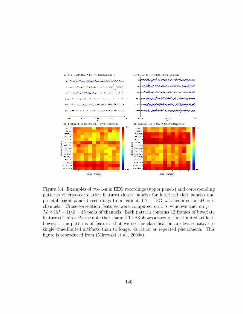
(a) EEG on 06-Dec-2001, 12:00 (interictal) (c) EEG on 12-Dec-2001, 06:20 (preictal)

(b) Features C on 06-Dec-2001, 12:00 (interictal) (d) Features C on 12-Dec-2001, 06:20 (preictal)

channel pairs

channel pairs

Time (frames) Time (frames)

Figure 5.4: Examples of two 1-min EEG recordings (upper panels) and correspondingpatterns of cross-correlation features (lower panels) for interictal (left panels) andpreictal (right panels) recordings from patient 012. EEG was acquired on M = 6channels. Cross-correlation features were computed on 5 s windows and on p =M × (M − 1)/2 = 15 pairs of channels. Each pattern contains 12 frames of bivariatefeatures (1 min). Please note that channel TLB3 shows a strong, time-limited artifact;however, the patterns of features that we use for classification are less sensitive tosingle time-limited artifacts than to longer duration or repeated phenomena. Thisfigure is reproduced from (Mirowski et al., 2009a).

140

Chapter 6

Application to Statistical Language Modeling

Whenever I fire a linguist our system

performance improves

At IBM Research in Speech Recognition

Frederick Jelinek

Accepting [...] that I really said it, I must

first of all affirm that I never fired anyone,

and a linguist least of all.

In “Some of My Best Friends Are Linguists"

Jelinek (2005)

Frederick Jelinek

This final applications chapter presents an adaptation of Dynamical Factor Graphs

for language modeling. It was presented at the IEEE Spoken Language Technology

workshop in December 2010 (Mirowski et al., 2010a), has been submitted for publica-

tion, and is the object of a patent application filed by AT&T Labs Research (Mirowski

et al., 2010b). Because we are trying to model discrete events (words) using hidden

variables, we resort to a major simplification in the latent variable inference. The

141

observation model is now simply a lookup table, which maps a 100-dimensional hid-

den vector to each word of the vocabulary, and contains no energy term. There is

no proper relaxation on the hidden variables either, therefore we cannot call them

latent anymore. On the upside, we gain the ability of full energy-based learning on

the dynamics.

Probabilistic models of text such as n-grams require an exponential number of

examples as the size of the context grows - a problem that is due to the discrete

word representation. They were recently outperformed by language models that use

a continuously valued and low-dimensional representation of words. In these models

word probabilities result from non-linear dynamics in the latent space. We propose

to build on Log-Bilinear models, and to enrich them with additional inputs such

as part-of-speech tags, almost-parsed supertags, a mixture topic model and by using

graph constraints based on word similarity. We demonstrate that our additions result

in significantly lower perplexity on different text corpora, as well as improved word

accuracy rate on speech recognition tasks, as compared to state-of-the-art N-gram

and existing continuous language models.

6.1 Statistical Language Modeling

A key problem in natural language processing (both written and spoken) is designing

a metric to score sentences according to their well-formedness in a language, also

known as statistical language modeling. In speech recognition applications, statistical

language models are generally used to rank the list of candidate hypotheses that are

generated based on acoustic match to the input speech. An example is N -gram

language models which assume that the probability of a word wt depends only on a

short, fixed history wt−1t−n+1 of n− 1 previous words (a Markov approximation). This

142

results in the joint likelihood of a sequence of T words being given by:

P(wT

1

)= P

(wn−1

1

) T∏

t=n

P(wt|wt−1

t−n+1

)(6.1)

The conditional probabilities in N -gram models are estimated by keeping track of

the n-gram counts in a training corpus. Their main limitation is that as the size of the

history increases, the size of the corpus needed to reliably estimate the probabilities

grows exponentially. In order to overcome this sparsity, back-off mechanisms (Katz,

1987) are used to approximate nth order statistics with lower-order ones, and sparse

or missing probabilities may be further approximated by smoothing (Chen and Good-

man, 1996).

In contrast to discrete n-gram models, recently-developed Continuous Statistical

Language Models (CSLM) (Bengio et al., 2003; Morin and Bengio, 2005; Schwenk

and Gauvain, 2003; Schwenk, 2010; Blitzer et al., 2004; Mnih and Hinton, 2007, 2008;

Mnih et al., 2009; Collobert and Weston, 2008; Sarikaya et al., 2010) embed the words

of the |W |-dimensional vocabulary into a low-dimensional and continuously valued

space <|Z|, and rather than making predictions based on the sequence of discrete

words wt, wt−1, . . . , w1 operate instead on the sequence of embedded word vectors

zt, zt−1, . . . , z1. The advantage of such models over discrete n-gram models is that

they allow for a natural way of smoothing for unseen n-gram events. Furthermore,

the representations for the words are discriminatively trained in order to optimize the

word prediction task.

In this paper, we describe a novel CSLM that extends previously presented models.

First, our model is capable of incorporating similarity graph constraints on word

representations. Second, the model can efficiently use word meta-features, like part-

of-speech tags or “almost parse” supertags (fragments of parse trees). Finally, the

143

model is also flexible enough to handle long range information derived from topic

models. Thus our architecture synthesizes and extends many of the strengths of the

state-of-the-art CSLMs (see Figure 6.1). While language modeling is our task and

hence test perplexity is a natural evaluation metric, we also evaluate our model on

word accuracy for speech recognition.

6.2 Proposed Extensions to Continuous Statistical

Language Modeling

The best-known CSLM is the Neural Probabilistic Language Model (NPLM) (Bengio

et al., 2003), which consists of a neural network that that takes as input a word

window history, embeds this in latent space, zt−1t−n+1 and is trained to directly predict

the probability of the next word wt (the probability is over the entire vocabulary).

Trainable parameters of this system are both the word embedding function (the way

in which words, wt are projected to their low-dimensional representations, zt) as well

as the network combination weights (how the z’s in the context are combined to

make the prediction). A variant of this model has been successfully applied to speech

recognition (Schwenk and Gauvain, 2003) and machine translation (Schwenk, 2010).

Since the NPLM architecture does not allow constraints to be added to the word

embeddings, we only adopt from this methods the non-linear architecture (single

hidden layer neural network) and the trainability of the embedding. Instead we base

our model on the Log-BiLinear (LBL) architecture (Mnih and Hinton, 2007, 2008;

Mnih et al., 2009). This probabilistic energy-based model is trained to predict the

embedding zt of the next word wt. The key elements of the LBL architecture are

explained in Sections 6.3.1, 6.3.2 and 6.3.3. We demonstrate in Section 6.4.2, that

144

LBL models outperform n-gram language models.

Other nonlinear classifiers (hierarchical logistic regression (Blitzer et al., 2004)) or

state-space models (Tied-Mixture Language Models, (Sarikaya et al., 2010)) used for

CSLM have been considered that initialize the word representation by computing a

square word co-occurrence matrix (bigrams) and reducing its dimensionality through

Singular Value Decomposition to the desired number of hidden factors |Z|. We fol-

low this work in initializing the LBL word embeddings as explained in Section 6.3.4.

We also explain there how one can impose similarity constraints on the word rep-

resentation, using for instance information about word similarity from the WordNet

taxonomy.

A third, major extension of our LBL model (section 6.3.5), is our incorporation of

part-of-speech tag features as additional inputs, similar to the Deep Neural Networks

with Multitask Learning (Collobert and Weston, 2008). The latter study, however,

addresses different supervised NLP tasks other than language modeling. We also

investigated the use of supertags, which are multi-level elements of a Tree-Adjoining

Grammar (Joshi, 1987).

Finally, in Section 6.3.7, we investigate the influence of the long-range depen-

dencies between words in the current and few previous sentences, or in the current

document. For this reason, we integrate our CSLM with unsupervised topic mod-

els for text, in a spirit similar to HMM-LDA (Griffiths et al., 2005).1 All the four

proposed improvements over LBL are evaluated both in terms of language model

perplexity and of speech recognition word accuracy in section 6.4.1Their language model was a simple discrete bigram.

145

6.3 Architecture of Our Statistical Language Model

with Hidden Variables

In a typical Continuous Statistical Language Model one tries to compute the proba-

bility distribution of the next word in a sequence using the distributed representation

of the preceding words. One class of models tries to achieve this by capturing the

dependencies/interactions between the distributed representation of the next word

and the distributed representations of the preceding words in the sequence. This is

achieved by defining an energy function (a cost) between the variables that capture

these dependencies. Learning in such models involves adjusting the parameters such

that low energies are assigned to the valid sequences of words and high energies to the

invalid ones. This is typically achieved by maximizing the likelihood of the training

corpus (LeCun et al., 2006).

6.3.1 Log-BiLinear Language Models

Log-Bilinear models, recently proposed by Mnih et al. in (Mnih and Hinton, 2007,

2008; Mnih et al., 2009) form our basic model class. Let us denote by wT1 = [w1 . . . wT ]

a discrete word sequence of length T , and its corresponding low dimensional real-

valued representation by zT1 = [z1 . . . zT ] (where ∀t, zt ∈ <|Z|). The LBL model tries

to predict the distributed representation of the next word zt. It outputs zt using a

linear function of the distributed representations of the preceding words zt−1t−n+1, where

zt−1t−n+1 denotes a stacked history of the previous word embedding (a vector of length

(n− 1)|Z|):

zt = Czt−1t−n+1 + bC = fC

(zt−1t−n+1

)(6.2)

146

Matrix C is a learnable parameter matrix that expresses the bilinear interactions

between the distributed representations of the previous words and the representation

of the current word. The vector bC is the corresponding vector of biases. For any

word wv in the vocabulary with embedding zv, the energy associated with respect to

the current sequence is a bilinear function and is given by:

E(t, v) = −zTt zv − bv (6.3)

Intuitively, this energy can be viewed as expressing the similarity between the

predicted distributed representation of the current word, and the distributed repre-

sentation of any other word wv in the vocabulary. The similarity is measured by the

dot product between the two representations. Using these energies one can assign the

probabilities to all the words wv in the vocabulary:

P(wt = wv|wt−1

t−n+1

)=

e−E(t,v)

∑|W |v′=1 e

−E(t,v′). (6.4)

Training an LBL model involves maximizing the likelihood of all the words in a

corpus, treating each word as a target. This is equivalent to minimizing the negative

log likelihood Lt over a data set:

Lt = E(t, v) + log

|W |∑

v′=1

e−E(t,v′). (6.5)

6.3.2 Non-Linear Extension to LBL

The LBL model as described above is capable of capturing only linear interactions

between representations of the previous words and the representation of the next

147

word, via the matrix C. However, expressing it as an energy-based model allows us

to add more complex interactions among the representations just as easily. This is

achieved by simply increasing the complexity of the energy function. For instance,

one can capture non-linear dependencies among the representations of the previous

words, and the next word by adding a single hidden layer neural network, as proposed

in (Mnih et al., 2009). In particular let matrices A and B be the two learnable

parameter matrices and the vectors bA and bB be the corresponding biases. Let

σ denote the tanh sigmoid transfer function which acts on hidden layer outputs.

Then the prediction given by this nonlinear component, which captures non-linear

dependencies among representations, is given by:

fA,B

(zt−1t−n+1

)= Bσ(Azt−1

t−n+1 + bA) + bB. (6.6)

Then, prediction by both the linear and the non-linear component of the LBL

(LBLN) is given by the sum of the two terms:

zt = fA,B

(zt−1t−n+1

)+ fC

(zt−1t−n+1

). (6.7)

The energy of the system is defined in exactly the same way as in equation (6.3),

and the loss function is defined in the same way as in equation (6.5). The system is

again trained by maximizing the likelihood of the training corpus.

6.3.3 Training the LBL(N) Model

Throughout this study the dimensions of the distributed representation of words was

set to |Z| = 100, and the number of hidden units in the neural network were set to

148

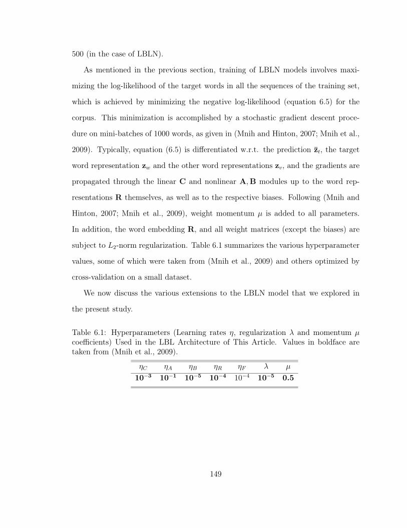
500 (in the case of LBLN).

As mentioned in the previous section, training of LBLN models involves maxi-

mizing the log-likelihood of the target words in all the sequences of the training set,

which is achieved by minimizing the negative log-likelihood (equation 6.5) for the

corpus. This minimization is accomplished by a stochastic gradient descent proce-

dure on mini-batches of 1000 words, as given in (Mnih and Hinton, 2007; Mnih et al.,

2009). Typically, equation (6.5) is differentiated w.r.t. the prediction zt, the target

word representation zw and the other word representations zv, and the gradients are

propagated through the linear C and nonlinear A,B modules up to the word rep-

resentations R themselves, as well as to the respective biases. Following (Mnih and

Hinton, 2007; Mnih et al., 2009), weight momentum µ is added to all parameters.

In addition, the word embedding R, and all weight matrices (except the biases) are

subject to L2-norm regularization. Table 6.1 summarizes the various hyperparameter

values, some of which were taken from (Mnih et al., 2009) and others optimized by

cross-validation on a small dataset.

We now discuss the various extensions to the LBLN model that we explored in

the present study.

Table 6.1: Hyperparameters (Learning rates η, regularization λ and momentum µcoefficients) Used in the LBL Architecture of This Article. Values in boldface aretaken from (Mnih et al., 2009).

ηC ηA ηB ηR ηF λ µ

10−3 10−1 10−5 10−4 10−4 10−5 0.5

149

6.3.4 Extension 1: Constraining the Hidden Word Embed-

dings

All the parameters A,B,C,R are initialized randomly. We use the rule of thumb

of generating zero-mean normally distributed words of variance equal to the inverse

of the matrix fan-in (LeCun et al., 1998b). Biases are initialized to zero, with the

exception of bv, which are initially equal to the unigram statistics of the training data.

Some CSLM architectures (Blitzer et al., 2004; Sarikaya et al., 2010) are however

dependent on the initial hidden word representation, and in order to evaluate this

dependency, we followed a procedure similar to (Sarikaya et al., 2010) which initializes

R using Singular Value Decomposition on the bi-gram (n-gram) co-occurrence matrix.

As can be shown in section 6.4.4, the low-dimensional nature of the word em-

bedding in CSLMs (|Z| << |W |, with |Z| = 100 and |W | typically over 10,000)

and the word co-occurrence in the text tend to cluster word representations zw

according to their syntactic co-occurrence and semantic equivalence. In order to

speed-up the learning of our model and to potentially help achieve better perfor-

mance, we considered imposing a graph constraint on the words. For each word w,

we defined its neighborhood Nw obtained through the hierarchical WordNet2 tree

and using the WordNet::Similarity module3 (specifically, we used Resnik similar-

ity (Resnik, 1999), keeping in Nw only words whose Resnik score was higher than

8). During learning time, the graph constraint was imposed by adding a penalty

term γ∑|W |

w=1 ‖ zw − 1|Nv |

∑v∈Nw

zv ‖22 to the total log-likelihood (we set γ = 1).

2See http://wordnet.princeton.edu3Available at http://wn-similarity.sourceforge.net/

150

6.3.5 Extension 2: Adding Part-Of-Speech Tags

The most important improvement over the LBL (Mnih and Hinton, 2007) and the

LBLN (Mnih et al., 2009) was the addition of Part-of-Speech (POS) tags to each word.

Conceptually, this step is identical to the word embedding: for each word, discrete

POS tags (out of a vocabulary of |X|, here between 30 and 52) are mapped into a

low-dimensional embedding <|ZX | through a linear operation (matrix F). The matrix

F was also initialized randomly in the same way as discussed in Section 6.3.4. We also

considered the case |X| = |ZX |, with an identity transform F = I|X|. Those tags can

then be concatenated with the |ZW |-dimensional word representations into a history

of n−1 word and feature representations, and used as an input to the predictive model

(Figure 6.1), just like in (Collobert and Weston, 2008). As explained below, POS tag

features can be trivially extended to accommodate other types of word features.

6.3.6 Extension 3: Incorporating Supertags

Supertags are elementary trees of a lexicalized tree grammar such as a Tree-Adjoining

Grammar (TAG) (Joshi, 1987). Unlike context-free grammar rules which are single

level trees, supertags are multi-level trees which encapsulate both predicate-argument

structure of the anchor lexeme (by including nodes at which its arguments must

substitute) and morpho-syntactic constraints such as subject-verb agreement within

the supertag associated with the anchor. There are a number of supertags for each

lexeme to account for the different syntactic transformations (relative clause, wh-

question, passivization etc.). For example, the verb give will be associated with at

least these two trees, which we will call tdi and tdi-dat, illustrated below:

151

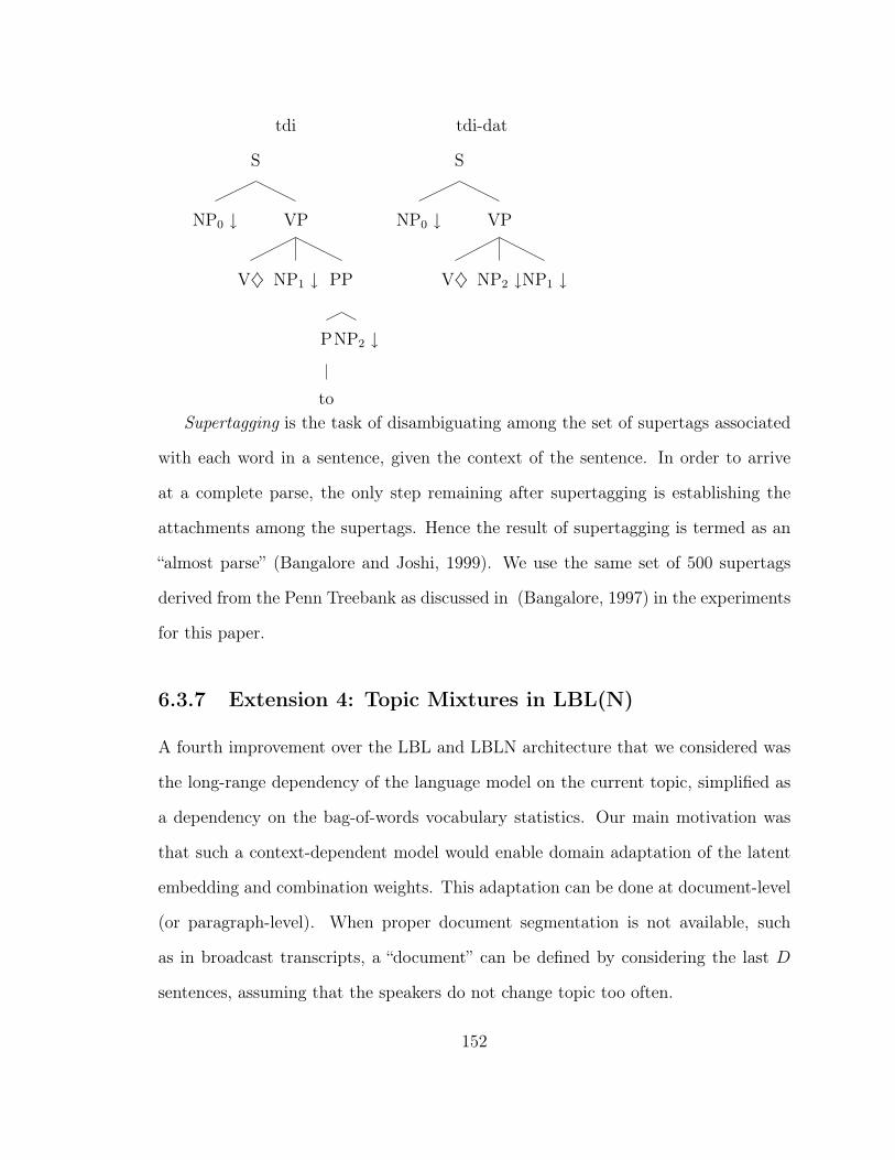
tdi tdi-dat

S

NP0 ↓ VP

V♦ NP1 ↓ PP

P

to

NP2 ↓

S

NP0 ↓ VP

V♦ NP2 ↓NP1 ↓

Supertagging is the task of disambiguating among the set of supertags associated

with each word in a sentence, given the context of the sentence. In order to arrive

at a complete parse, the only step remaining after supertagging is establishing the

attachments among the supertags. Hence the result of supertagging is termed as an

“almost parse” (Bangalore and Joshi, 1999). We use the same set of 500 supertags

derived from the Penn Treebank as discussed in (Bangalore, 1997) in the experiments

for this paper.

6.3.7 Extension 4: Topic Mixtures in LBL(N)

A fourth improvement over the LBL and LBLN architecture that we considered was

the long-range dependency of the language model on the current topic, simplified as

a dependency on the bag-of-words vocabulary statistics. Our main motivation was

that such a context-dependent model would enable domain adaptation of the latent

embedding and combination weights. This adaptation can be done at document-level

(or paragraph-level). When proper document segmentation is not available, such

as in broadcast transcripts, a “document” can be defined by considering the last D

sentences, assuming that the speakers do not change topic too often.

152

We decided to implement a topic model based on the popular Latent Dirichlet

Allocation4 (Blei et al., 2003), a graphical model that is trained to extract a word-

topic matrix from a collection of documents, and that can infer latent topic posterior

distributions θd for each test document d. As can be seen on Fig. 6.1, the K-

dimensional topic vector (where∑

k θk = 1) can be used as weights of a mixture model.

Because the predictions made by each component of the mixture add-up for the final

prediction zt (6.8), the implementation of the topic-dependent LBL(N) architecture

is a simple extension of the previously described LBLN-based architectures.

zt =K∑

k=1

θk(fCk

(zt−1t−n+1

)+ fAk,Bk

(zt−1t−n+1

))(6.8)

As can be seen in the next section, adding a topic model mixture holds promise in

terms of language model perplexity but still requires additional experimental evalua-

tion.

Note that we could have used the topic model developed in Chapter 5 of my

thesis, but we initially preferred an out-of-the-box solution provided by LDA. Another

reason for our choice of topic models was the fact that LDA computes a topic simplex

(multinomial distribution over topics) which is very handy for mixture model weights.

6.4 Results Obtained with Feature-Rich Log-BiLinear

Language Model

The following section summarizes several sets of experiments performed on four dis-

tinct datasets (section 6.4.1), aimed at assessing the test set perplexity of the respec-

tive language models (section 6.4.2), and at measuring the word accuracy performance4We used the Gibbs-based implementation of LDA, available at http://gibbslda.sourceforge.net/

153

for speech recognition tasks (section 6.4.3). Finally, we illustrate the power of clus-

tering words with low-dimensional representations (section 6.4.4).

6.4.1 Language Corpora

We have evaluated our models on five distinct, public datasets: 1) the Airline Travel

Information System (ATIS), a small corpus containing short sentences concerning air

travel, 2) the Wall Street Journal (WSJ) set, containing sentences from business news,

3) the Reuters-21578 corpus5 of business news articles, which is normally used for text

categorization, 4) TV broadcast news transcripts HUB-4 from the LDC (reference

2000S88), with audio information, and 5) the large AP News corpus used in (Bengio

et al., 2003; Mnih and Hinton, 2007, 2008; Mnih et al., 2009). Table 6.2 summarizes

the statistics of each dataset.

For the WSJ set, we used POS tags to identify and replace all numbers (tag CD)

and proper nouns (tags NNP and NNPS), as well as words with 3 or fewer occurrences,

by generic tags resulting in a considerable reduction in the vocabulary size. For

the Reuters set, each article was split into sentences using the Maximum Entropy

sentence-splitter by Adwait Ratnaparkhi6, and then tagged using the Stanford Log-

linear Part-of-Speech Tagger7. We replaced numbers and rare words (i.e. appearing

less than four times) by special tags, as well as out-of-vocabulary test words by unk.

For the HUB-4 corpus, we obtained 100-best hypotheses for each audio file in the test

set using a speech recognition system comprising of a trigram language model that

was trained on about 813,975 training sentences. In all the experiments but on AP

News, 5% of the training data were set apart during learning for cross-validation

(the model with the best performance on the cross-validation set was retained). The5See: http://disi.unitn.it/moschitti/corpora.htm6See: http://sites.google.com/site/adwaitratnaparkhi/7See: http://nlp.stanford.edu/software/tagger.shtml

154

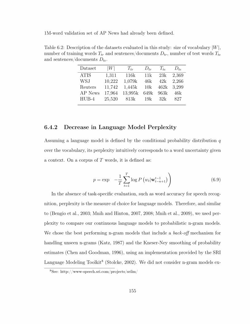
1M-word validation set of AP News had already been defined.

Table 6.2: Description of the datasets evaluated in this study: size of vocabulary |W |,number of training words Ttr and sentences/documents Dtr, number of test words Tteand sentences/documents Dte.

Dataset |W | Ttr Dtr Tte Dte

ATIS 1,311 116k 11k 23k 2,369WSJ 10,222 1,079k 46k 42k 2,266Reuters 11,742 1,445k 10k 462k 3,299AP News 17,964 13,995k 649k 963k 46kHUB-4 25,520 813k 19k 32k 827

6.4.2 Decrease in Language Model Perplexity

Assuming a language model is defined by the conditional probability distribution q

over the vocabulary, its perplexity intuitively corresponds to a word uncertainty given

a context. On a corpus of T words, it is defined as:

p = exp

(− 1

T

T∑

t=1

logP(wt|wt−1

t−n+1

))

(6.9)

In the absence of task-specific evaluation, such as word accuracy for speech recog-

nition, perplexity is the measure of choice for language models. Therefore, and similar

to (Bengio et al., 2003; Mnih and Hinton, 2007, 2008; Mnih et al., 2009), we used per-

plexity to compare our continuous language models to probabilistic n-gram models.

We chose the best performing n-gram models that include a back-off mechanism for

handling unseen n-grams (Katz, 1987) and the Kneser-Ney smoothing of probability

estimates (Chen and Goodman, 1996), using an implementation provided by the SRI

Language Modeling Toolkit8 (Stolcke, 2002). We did not consider n-gram models ex-8See: http://www-speech.sri.com/projects/srilm/

155

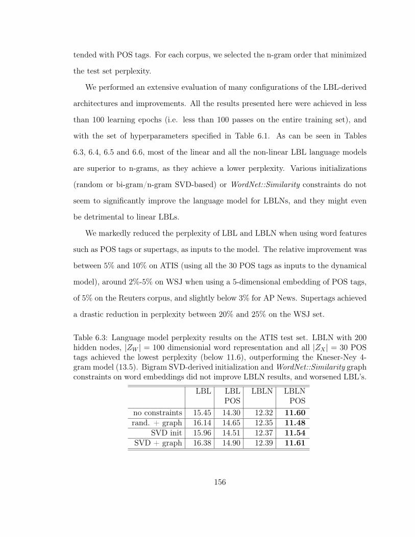
tended with POS tags. For each corpus, we selected the n-gram order that minimized

the test set perplexity.

We performed an extensive evaluation of many configurations of the LBL-derived

architectures and improvements. All the results presented here were achieved in less

than 100 learning epochs (i.e. less than 100 passes on the entire training set), and

with the set of hyperparameters specified in Table 6.1. As can be seen in Tables

6.3, 6.4, 6.5 and 6.6, most of the linear and all the non-linear LBL language models

are superior to n-grams, as they achieve a lower perplexity. Various initializations

(random or bi-gram/n-gram SVD-based) or WordNet::Similarity constraints do not

seem to significantly improve the language model for LBLNs, and they might even

be detrimental to linear LBLs.

We markedly reduced the perplexity of LBL and LBLN when using word features

such as POS tags or supertags, as inputs to the model. The relative improvement was

between 5% and 10% on ATIS (using all the 30 POS tags as inputs to the dynamical

model), around 2%-5% on WSJ when using a 5-dimensional embedding of POS tags,

of 5% on the Reuters corpus, and slightly below 3% for AP News. Supertags achieved

a drastic reduction in perplexity between 20% and 25% on the WSJ set.

Table 6.3: Language model perplexity results on the ATIS test set. LBLN with 200hidden nodes, |ZW | = 100 dimensionial word representation and all |ZX | = 30 POStags achieved the lowest perplexity (below 11.6), outperforming the Kneser-Ney 4-gram model (13.5). Bigram SVD-derived initialization andWordNet::Similarity graphconstraints on word embeddings did not improve LBLN results, and worsened LBL’s.

LBL LBL LBLN LBLNPOS POS

no constraints 15.45 14.30 12.32 11.60rand. + graph 16.14 14.65 12.35 11.48

SVD init 15.96 14.51 12.37 11.54SVD + graph 16.38 14.90 12.39 11.61

156

Taking advantage of the small size of the ATIS dataset, we investigated the influ-

ence of several hyper-parameters on the performance of the LBL model: the linear

model learning rate ηC , as well as the word embedding learning rate ηR, the first layer

ηA and second layer ηB nonlinear module learning rates. We conducted an exhaustive

search on a coarse grid of the above hyper-parameters, assuming an LBL(N) archi-

tecture with |ZW | = 100 dimensional word representation and |H| = 0, 50, 100 or

200 hidden nonlinear nodes, as well as |ZX | = 0 or 3 dimensional embedding of POS

tag features. Evidently, as suggested in (Mnih et al., 2009), the number of hidden

non-linear nodes had a positive influence on the performance, and our addition of

POS tags were beneficial to the language model. Regarding the learning rates, the

most sensitive rates were ηR and ηC , then ηA and finally ηB. The optimal results were

achieved for the hyper-parameter values in Table 6.1. We then selected the optimal

LBLN architecture with |ZW | = 100 and |H| = 200 and further evaluated the joint

influence of the feature learning rate ηF , the graph constraint coefficient γ, the di-

mension of the POS tag embedding |ZX |, and the random or bigram initialization of

the word embeddings. The most important factor was ηF , which needed to be smaller

than 10−3, and the presence or absence of POS features (larger embedding sizes did

not seem to significantly improve the model).

In a subsequent set of experiments, we evaluated the benefit of adding a topic

model to the (syntactic) language model, focusing on the Reuters and AP News

datasets (organized in documents) and on the HUB-4 transcripts (a window of five

consecutive sentences was treated as a document; results reported in section 6.4.3).

We used the standard Latent Dirichlet Allocation topic model to produce a simplex

of topic posteriors θt,1, . . . , θt,K for K = 5 topics, for each “document”, and used

these coefficients as weights of a 5-mixture model. We retained, for each mixture

component, the same LBL and LBLN architectures as in the previous experiments,

157

Table 6.4: Language model perplexity results on the WSJ test set. Kneser-Ney 5-grams attain a perplexity of 86.53. Similar architectures to the one in Table 6.5were used. While the benefit of initializing the word representation and enforcingWordNet::Similarity graph constraints (noted as R) is not obvious, POS tags clearlyreduce the perplexity of LBL and LBLN, and supertags are even better. We controlfor the size |ZX | of the feature embedding, showing that supertags are far superiorto POS tags. Learning was stopped after 100 epochs, and results in italics show LBLmodels that did not reach their optimum.

LBL LBL LBLN LBLNR R

No features 93.4 98.0 84.9 84.4|ZX |POS = 5 90.3 95.8 82.6 81.1|ZX |POS = 50 88.7 93.5 83.0 82.6|ZX |super = 50 69.6 72.4 66.7 66.3

and experimented with adding POS features. As Table 6.5 suggests, adding a topic

model improved the plain LBL perplexity (but not LBLN’s) on the medium-size

Reuters set, and it significantly improved the perplexity on the large AP News corpus

(the combined topic+POS reduction in perplexity was 8% on both LBL and LBLN).

6.4.3 Increase in Speech Recognition Word Accuracy

In Table 6.7, we present the results of speech recognition experiments using our

language model. We used AT&T Watson ASR (Goffin et al., 2005) (with a trigram

language model trained on HUB-4 training set) to produce 100-best hypotheses for

each of the test audio files of the HUB-4 task. The 1-best and the 100-best oracle

word accuracies are 63.7% and 66.6% respectively. Using a range of language models

(including a 4-gram discrete LM), we re-ranked the 100-best hypotheses according

to LM perplexity (ignoring the scores from ASR), and selected the top one from

each list. The top-ranking hypothesis resulting from LBLN models had significantly

better word accuracies than any discrete language models. Adding a topic mixture

158

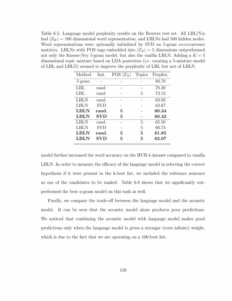
Table 6.5: Language model perplexity results on the Reuters test set. All LBL(N)shad |ZW | = 100 dimensional word representation, and LBLNs had 500 hidden nodes.Word representations were optionally initialized by SVD on 5-gram co-occurrencematrices. LBLNs with POS tags embedded into |ZX | = 5 dimensions outperformednot only the Kneser-Ney 5-gram model, but also the vanilla LBLN. Adding a K = 5dimensional topic mixture based on LDA posteriors (i.e. creating a 5-mixture modelof LBL and LBLN) seemed to improve the perplexity of LBL but not of LBLN.

Method Init. POS |ZX | Topics Perplex.5-gram - - - 80.78LBL rand. - - 78.30LBL rand. - 5 73.12LBLN rand. - - 63.92LBLN SVD - - 63.67LBLN rand. 5 - 60.34LBLN SVD 5 - 60.42LBLN rand. - 5 65.50LBLN SVD - 5 66.74LBLN rand. 5 5 61.85LBLN SVD 5 5 62.07

model further increased the word accuracy on the HUB-4 dataset compared to vanilla

LBLN. In order to measure the efficacy of the language model in selecting the correct

hypothesis if it were present in the k-best list, we included the reference sentence

as one of the candidates to be ranked. Table 6.8 shows that we significantly out-

performed the best n-gram model on this task as well.

Finally, we compare the trade-off between the language model and the acoustic

model. It can be seen that the acoustic model alone produces poor predictions.

We noticed that combining the acoustic model with language model makes good

predictions only when the language model is given a stronger (even infinite) weight,

which is due to the fact that we are operating on a 100-best list.

159

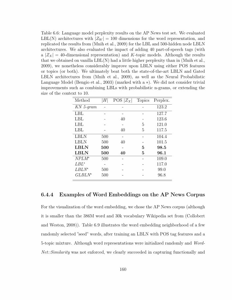
Table 6.6: Language model perplexity results on the AP News test set. We evaluatedLBL(N) architectures with |ZW | = 100 dimensions for the word representation, andreplicated the results from (Mnih et al., 2009) for the LBL and 500-hidden node LBLNarchitectures. We also evaluated the impact of adding 40 part-of-speech tags (witha |ZX | = 40-dimensional representation) and K-topic models. Although the resultsthat we obtained on vanilla LBL(N) had a little higher perplexity than in (Mnih et al.,2009), we nonetheless considerably improve upon LBLN using either POS featuresor topics (or both). We ultimately beat both the state-of-the-art LBLN and GatedLBLN architectures from (Mnih et al., 2009), as well as the Neural ProbabilisticLanguage Model (Bengio et al., 2003) (marked with a ∗). We did not consider trivialimprovements such as combining LBLs with probabilistic n-grams, or extending thesize of the context to 10.

Method |H| POS |ZX | Topics Perplex.KN 5-gram - - - 123.2LBL - - - 127.7LBL - 40 - 123.6LBL - - 5 121.0LBL - 40 5 117.5LBLN 500 - - 104.4LBLN 500 40 - 101.5LBLN 500 - 5 98.5LBLN 500 40 5 96.1NPLM∗ 500 - - 109.0LBL∗ - - - 117.0LBLN∗ 500 - - 99.0GLBLN∗ 500 - - 96.8

6.4.4 Examples of Word Embeddings on the AP News Corpus

For the visualization of the word embedding, we chose the AP News corpus (although

it is smaller than the 386M word and 30k vocabulary Wikipedia set from (Collobert

and Weston, 2008)). Table 6.9 illustrates the word embedding neighborhood of a few

randomly selected ”seed” words, after training an LBLN with POS tag features and a

5-topic mixture. Although word representations were initialized randomly and Word-

Net::Similarity was not enforced, we clearly succeeded in capturing functionally and

160

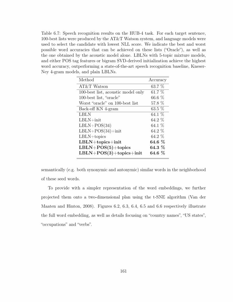
Table 6.7: Speech recognition results on the HUB-4 task. For each target sentence,100-best lists were produced by the AT&T Watson system, and language models wereused to select the candidate with lowest NLL score. We indicate the best and worstpossible word accuracies that can be achieved on these lists (“Oracle”), as well asthe one obtained by the acoustic model alone. LBLNs with 5-topic mixture models,and either POS tag features or bigram SVD-derived initialization achieve the highestword accuracy, outperforming a state-of-the-art speech recognition baseline, Kneser-Ney 4-gram models, and plain LBLNs.

Method AccuracyAT&T Watson 63.7 %100-best list, acoustic model only 61.7 %100-best list, “oracle” 66.6 %Worst “oracle” on 100-best list 57.8 %Back-off KN 4-gram 63.5 %LBLN 64.1 %LBLN+init 64.2 %LBLN+POS(34) 64.1 %LBLN+POS(34)+init 64.2 %LBLN+topics 64.2 %LBLN+topics+init 64.6 %LBLN+POS(5)+topics 64.3 %LBLN+POS(3)+topics+init 64.6 %

semantically (e.g. both synonymic and antonymic) similar words in the neighborhood

of these seed words.

To provide with a simpler representation of the word embeddings, we further

projected them onto a two-dimensional plan using the t-SNE algorithm (Van der

Maaten and Hinton, 2008). Figures 6.2, 6.3, 6.4, 6.5 and 6.6 respectively illustrate

the full word embedding, as well as details focusing on “country names”, “US states”,

“occupations” and “verbs”.

161

Table 6.8: Speech recognition results on HUB-4 transcripts. We used the same train-ing and test sets as in Table 6.7, but with the true sentence to be predicted includedamong the 101-best candidates.

Method AccuracyBack-off KN 4-gram 86.9 %LBLN+POS+init 94.0 %“Oracle” 100 %

6.4.5 Computational Requirements

We implemented our LBL-derived architectures under Matlab. The training was lin-

ear in the size of the dataset (i.e. the number of words). As observed for previous

CSLM models (Bengio et al., 2003) or (Mnih and Hinton, 2007), the bulk of the com-

putations consisted in evaluating the word likelihood (6.4) and in differentiating the

loss (6.5), which was theoretically linear in the size of the vocabulary |W |. However,

thanks to the BLAS and LAPACK numerical libraries, it was sublinear in practice.

Typically, training our LBL architectures on moderately sized datasets (WSJ, Reuters

and TV broadcasts) would take about a day on a multi-core server. Because of the

possible book-keeping overhead that might arise from sampling approximations, or

because of the decreased language model performance (higher perplexity) when hier-

archical word representation are used (Morin and Bengio, 2005), or of the LBL (Mnih

and Hinton, 2008), we restrict ourselves to the exact solution.

6.5 Conclusions

We presented an energy based statistical language model with a flexible architec-

ture that allows for novel and diverse extensions of the log-bilinear model formulated

in (Mnih and Hinton, 2007, 2008; Mnih et al., 2009). We also explored initializations

162

Table 6.9: Examples of 10 closest neighbors in the <100 word embedding space onAP News. We used the best LBLN+POS+topics architecture from Table 6.6. The 7seed words were selected randomly, and cosine similarity was used to compare anytwo word vectors.

frustrations tried immune marblefeelings stopped harmful graniteachievements threatened resistant velvetaccomplishments sought susceptible bronzeadvantages decided prone silkorigins returned addictive leathervigor met abnormal flowersuccesses moved transmitted mahoganyweaknesses kept unsafe brickstrength refused beneficial neonenthusiasm offered harmless wooden

crime_rate technologies savings_and_loanswork_force industries thriftstandard_of_living systems law_firminflation_rate foods estatebudget_deficit brands investment_companyunemployment_rate carriers real_estatedemise laboratories transactionstock_market suppliers bank_accountpeso enterprises guarantyvalue products cartelnet methods corporation

of word embeddings and word similarity constraints via a word-graph, with mixed

results, but we demonstrated consistent and significant predictive improvements by

incorporating part-of-speech tags or supertags as word features, as well as long range

(document level) topic information. Our results show that our model significantly

advances the state-of-the-art, beating both n-gram models and the best continuous

language models on test perplexity. Finally, we demonstrated the utility of this im-

proved language modeling by obtaining better word accuracy on a speech recognition

task.

163

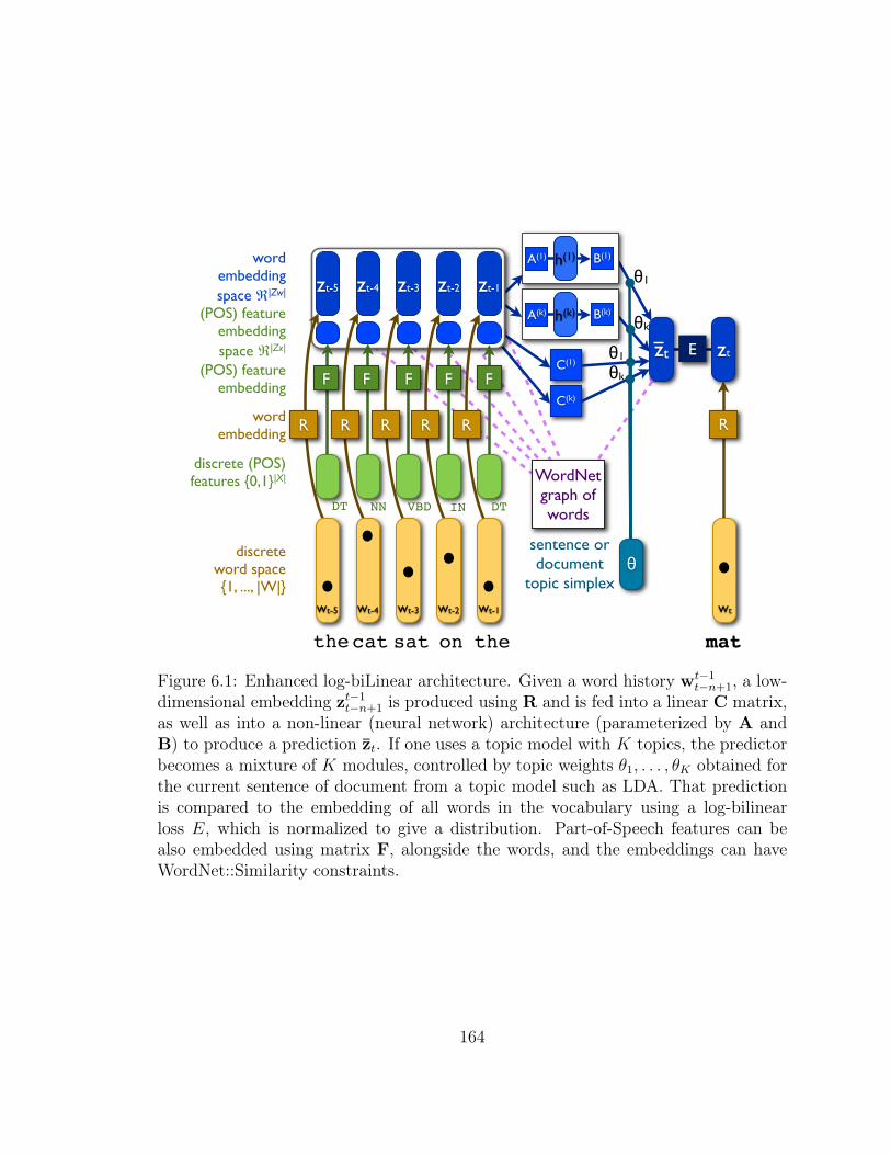
WordNet graph of words

C(k)

A(k) B(k)h(k)

C(1)

thecat sat on the mat

DT NN VBD IN DT

R R R R R

F F F F F

wordembeddingspace ℜ|Zw|

discreteword space1, ..., |W|

discrete (POS)features 0,1|X|

(POS) featureembeddingspace ℜ|Zx|

(POS) featureembedding

wordembedding

A(1) B(1)h(1)

E

R

θ1

θ1θk

θk

θsentence ordocument

topic simplex

zt-5 zt-4 zt-3 zt-2 zt-1

zt zt

wt-5 wt-4 wt-3 wt-2 wt-1 wt

Figure 6.1: Enhanced log-biLinear architecture. Given a word history wt−1t−n+1, a low-

dimensional embedding zt−1t−n+1 is produced using R and is fed into a linear C matrix,

as well as into a non-linear (neural network) architecture (parameterized by A andB) to produce a prediction zt. If one uses a topic model with K topics, the predictorbecomes a mixture of K modules, controlled by topic weights θ1, . . . , θK obtained forthe current sentence of document from a topic model such as LDA. That predictionis compared to the embedding of all words in the vocabulary using a log-bilinearloss E, which is normalized to give a distribution. Part-of-Speech features can bealso embedded using matrix F, alongside the words, and the embeddings can haveWordNet::Similarity constraints.

164

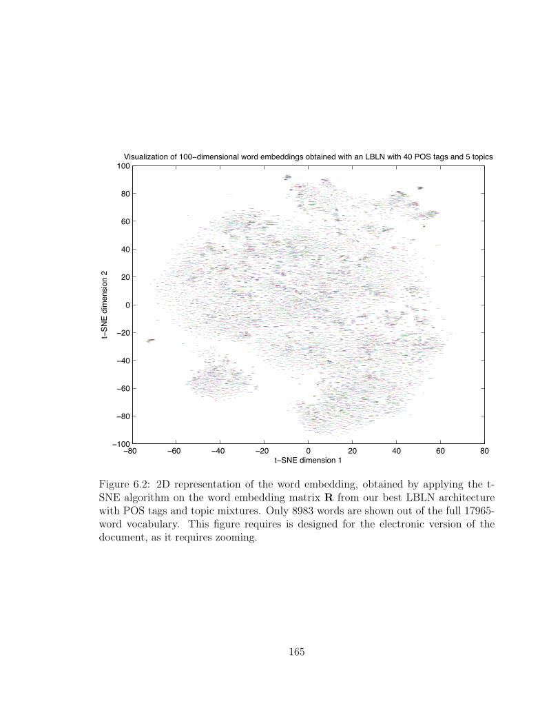
−80 −60 −40 −20 0 20 40 60 80−100

−80

−60

−40

−20

0

20

40

60

80

100

brain+cells

relief

stocks

slipping

come+on

empress

cousin

bathtub

formation

facility

floodwaters

referring

come+in

crazy

immune+system

round−trip

tumor

illustration

check

amendments

stockman

branches

satisfy

live+in

4+1

speeches

kindness

robbing

productions

local+government

abstract

porn

chaos

outlaw

stalled

last+name

circular

lettuce

urging

gilt

barren

niger

tearfully

updated

glimpse

dirt

space+shuttle

coerced

signed+on

grammar

salute

accomplices

bad+weather

roundup

month

upjohn

actions

erroneously

motorcade

columns

gestures

riding

retrieved

steer

complex

saigon

contingency

deficit

sydney

half+dozen

retarded

egyptian

situations

in+certain

speeding

as+it+is

sermon

reasoning

disaster+areas

banners

lorenz

resign

a+gain

stand+in

extract

lopsided

dose

explains

browner

turning+point

immune

upbeat

greek

juvenile

kampala

wilder

routinely

tries

tv+stations

slept

toll

disarray

keeping

minority+leader

interested

poultry

entertainment

semi

chain

element

pleasant

protease

foes

spacey

camouflage

side−by−side

testify

analyze

piled+up

diet

demise

highways

blizzards

opens

beckley

multicolored

recreation

inhalation

escort

convinced

accidental

communication

johnston

disability

boats

treats

primary+school

outbreak

complications

third

breathtaking

frenzied

travel+to

young

a+late

cases

owns

there+in

nuclear+explosions

raging

abducted

leak

faint

follows

march+17

get+out

treasures

answering+machine

proudly

gallery

inserted

repairing

general+agreement

actor

rosas

strip

conservative+party

properties

’’.

conscious

sealing

diverse

defender

cloth

generate

residences

louis

macedonia

cyclical

challenger

draft

privatization

promoter

malnutrition

theaters

drag tearing

twin

lsd

underscores

hamper

cabaret

minutes

overlooked

waits

zagreb

workplace

machine+gun

insurers

contributors

mother−in−law

junior

drilling

television+stations

luck

got+it

in+charge

guardian

surroundings

taxation

preparing

vacant

nov

incident

dismissing

port+arthur

training+program

dove

stay

charging

preoccupied

dual

intersections

threaten

legal+action

galbraith

scenarios

traffic+jams

military

bomb

sell

stand−in

netscape

turned+up

backgrounds

defeats

chased

allows

rolling

ga

wooden

commission

endanger

deals

easter

approving

oldest

fiber

airways

hart

intelligence

hunter

seventeen

hard

in+the+north

news+conference

polish

ran+into

europeans

guide

glance

wagon

handed+over

works+on

wallace

shop

undisclosed

patriotic

payoff

resisting

fortunately

boat

mob

convenience

private

described

adjacent

alike

aspect

luggage

blew

banner

medications

flowing

credit+card

centennial

mismanagement

royals

achievement

needed

reassigned

protester

tether

paraded

discontent

burdened

teddy

nearest

watch

seldom

cannon

loyalist

each+day

counting

refrained

mandela

cut+down

finishing

capacity

economic+growth

assailants

sponsor

earned

tamils

journey

rothschild

analyzing

court

have+on

freshly

broadcasters

rosa

reassured

in+person

moon

readers

civil+liberties

probably

col

finance+ministers

wind

her+a

sea+lions

no+matter

adjustments

contended

insider

heritage

industry+analysts

brasilia

contribution

judaism

pavement

massachusetts

square+feet

so−called

someday

sits+in

carbon

inter

conversation

astronomy

bounced

permit

plant

gin

wreaths

secretive

cloudy

awaited

regular

serbs

ecological

ranked

existed

euphoria

payroll

murphy

property+rights

pay+attention

calling+on

african+nation

unrelated

good+condition

obliged

wrath

time

high−powered

autos

downstream

prestigious

recommending

divorce

counseling

settling

interpreted

false+statements

pro−lifeblunt

volcanic

atop

advisers

caught+fire

tobacco+industry

accords

add+up

trick

nationalist

legally

encouragement

deliberations

mistake

intact

innovative

fundamental

costumes

hardship

outreach

hard+on

spell+out

ecuador

invasion

shores

professed

saw

agents

bus+driver

nitrogen

position

sixty−nine

work

taking

pieces

bailout

hungarian

holiest

sketches

bowed

cowboys

ignored

rainy

disband

day−to−day

straight

manufacture

mount

pornography

patrolling

on−line

fill

hammer

belgian

goes

liberal

amounts

bike

sweeping

washed

frigid

billboards

assemblyman

norman

school+year

steered

peanut

rebels

is

marquette

colleagues

took+in

against

abuses

roman+catholic

tied

siegfried

trans

aurora

january

provides

clergy

giveaway

came+up

influential

pioneers

honeymoon

peacefully

ailes

airliner

footing

relocate

brought+up

been+on

state+attorney

zaire

interior+department

types

slapped

soup

contribute

dell

route

span

sunfans

snow−covered

kingston

inroads

partisan

confidential

take+effect

involved+with

motown

workshop

folded

lackluster

irresponsible

zimmer

expansion

rationing

death+penalty

caused

took+out

kitchen+table

sincere

were+set

lacy

gloom

predecessor

neighbor

batons

spiritual

tightened

invention

immunization

weigh

pennsylvania

her+as

probation

san+juan

jokes

a+base

house+of+representatives

collisions

slave

ideological

region

own

spontaneous

saturday

awaits

origin

accent

bomber

taken+on

enrichment

simeon

pulled

harrowing

cynicism

some+day

globes

bordering

biologist

speeds

managing+editor

came+after

scientific

co−author

pre−trial

wave

causing

dividing

missouri

runaway

pierre

justices

herbert

in+view

ditch

law+practice

plans

smash

sued

tonight

unveiling

town+hall

securities

brewing

chores

fund

doomed

complain

inventories

liftoff

rescheduled

handed+down

jimenez

crusade

scattered

flooding

foods

blowing

brick

energy

forget

soybean

housing+project

reeve

permitted

beast

leaking

pamphlets

roadside

conn

catalogs

il

keepers

everywhere

grandmother

prediction

setting+off

haitian

soaring

fog

segregation

cooperated

awful

first+amendment

circulation

box−office

manila

blown+up

habits

deny

sadly

commonly

percent

imaging

correspondence

quito

lock

michael+jackson

teams

inadvertently

defenders

altering

compact

good+health

shovel

60+minutes

strapped

dropped+in

authored

diners

shortage

memorial

round

sections

adams

shark

brad

mammoth

reimbursement

hanoi

red+cross

forcefully

skull

sesame

puts

maneuvering

finding

bent+on

words

en+route

stealing

commando

miracles

belt

blow

newt

difference

denied

couple

secured

prohibition

grains

other+than

con

kicker

culture

copyright

fastest−growing

labor+secretary

retaliatory

asking+for

nobel+prize

nominee

perhaps

lutheran

rewrite

turns+out

chaotic

underlying

treasury

arias

amazon

secretary

detain

staffers

unanimous

laughter

ag

voucher

winnipeg

remedies

greene

cosmonaut

dame

directory

eyes

tycoon

eastward

descending

took+the+stand

patronage

pay+off

heaviest

air+pollution

approves

anti

pregnant

turn+in

withdrew

sponsored

sorry

bring+in

pocahontas

manchester

boycott

controversy

ensemble

jeopardized

patently

discourage

spain

bribery

cardboard

uniting

avert

accidents

kitchen

hampshire

meters

fruits

harvest

greatly

plaintiff

talking+to

boone

rule

stump+speech

chronic

prudent

beverly+hills

refer

going+through

freedoms

ethics+committee

recruits

reassuring

radical

hammered

event

flush

shaking

wildlife

talk+shows

antique

beloved

buses

put+off

major+league

went+out

obsessed

sort+of

child+support

climber

stalkedindict

bloom

ed

crude

welfare+state

oliver+stone

touch

brook

next

in+short

hotel

fanfare

distrust

milestone

quest+for

murray

characters

spinal

clip

diplomat

san+jose

learning

waive

assassinations

ruthless

transform

mo

quality

curtis

stuff

barrages

wonders

commencement

revoke

k

instrumental

estates

praise

clauses

warmly

ira

throwing

badly

leveled

comprise

stinging

under+controlbuying

examined

calgary

sprint

five

considers

billionaire

freezing

mi

signed+up

grew

priced

given+in

anti−tank

turin

30+minutes

embargo

e−mail

balances

carpenter

ruled

comedy

successfully

invoked

spies

launched

respective

preventing

a+nasa

american+stock+exchange

budapest

lufkin

ripe

warrant

breaks

sharpened

composer

opposing

appears

altar

toughest

hijacking

seth

inflated

passages

manual

file

slogans

structure

penguin

regularly

written

cooler

defective

remind

calmly

cheap

pity

device

bank+of+japan

asserting

feb.

detentions

gunshot

implant

at+a+time

plagued

theory

destroyed

drivers

gazette

tax+increases

painfully

emerges

classmate

homosexuals

peacemaking

cake

quick

came+on

brutal

riot

concert

dynamite

kosovo

harsh

escorts

streamline

individuals

laser

chieftains

settlement

notebook

in+principle

truck

neon

rushdie

investor

reform

banned

publicly

pirated

newest

midsection

am

graves

leaders

mostly

glamour

cadets

destabilize

notificationfax

thus+far

find+out

paperbacks

brief

conversations

genital

alter

newton

stuck+to

fractured

biology

became

western

countrymen

commemorative

opera+house

mountainous

breast+cancer

surely

rained

economies

david

serious

refineries

jan

gurney

assured

juries

show

get+off

beneficiaries

cavalry

ritual

cape+canaveral

each+week

enforcement

dissatisfaction

newsstands

killingsweep

quarterly

arbitrary

irish+republican+army

marshal

widely

duff

wall

adversaries

insults

acoustic

near

incorrect

spacecraft

sealed+off

little+rock

merely

atomic

crawled

persuade

causes

undergoing

toys

learned

blues

scud

caves

nursing

new+guinea

myth

copied

advantage

root+out

abraham

december

softening

fool

isolationist

chided

intrigued

videotape

interrogated

chittagong

walking

tv+show

bees

whether

parentheses

preserving

postwar

cut+to

disagree+with

unpleasant

castes

affiliates

buyers

attributed

reluctance

sobering

yellow

knocked+out

contested

called+in

taking+part

breaking

hunger

premiered

mixed+in

adoption

nowhere

curve

kenya

transmission

changing

habit

unemployment+rate

relocation

rope

go+on

sampled

pinpoint

works+in

produce

systematically

as+expected

removed

wasting

continues

eleven

stranger

comfortable

problems

high−risk

afterwards

telegraph

tunisia

army+base

rejected

jars

regime

fbi

missed

pay+back

ex−wife

elaborate

including

consistent

liked

compromise

malaysia

aisle

ghana

pitting

chefs

bunkers

counterparts

uprising

income+taxes

interpret

enhanced

sung

front−line

recruiting

resentment

based+on

inclusion

pandering

calls

patrolled

attempting

column

goodbye

copyrights

slow

pizza

withholding

n.m

thwart

sipping

special

called+off

fond

roles

state+troopers

flow

herman

radios

ranged

bigotry

belonged+to

bring+to

arming

the+devil

beatrice

was+having

iraq+is

exploits

principals

decades

fingerprints

cessation

filled

unsure

irons

bruce

agency

consistently

tennis

luxembourg

wire

canisters

widespread

moments

politburo

fascinating

lions

extremely

organic

helmet

prince

events

indian

reacted

on+his+own

take+advantage

election+day

weeks

regrettable lowering

upbringing

await

texas

managing

transmissions

turn+to

explosion

attitude

assistant

darling

classics

baptist

sailing

believes

carolina

zodiac

step+by+step

peoria

proving

tijuana

mustard

yard

fuller

digital

standoff

suggesting

biochemist

contact

back+down

feed

ways

covered

kansan

custody

orbit

rookie

plead

controversies

caucasus

initiative

fast−growing

qualifies

nigeria

israelis

u.s+army

sniffing

that+much

option

spikes

australia

belly

state+capital

advises

loneliness

throats

outlawed

disguised

predecessors

vigor

kaiser

irrational

hillary

saw+the

normal

meant

thirty−one in+between

high+blood+pressure

funk

guitar

incorporated

acclaim

thomas

rule+out

betting

bruised

unnecessary

line−item

sessions

defense+policy

examples

proven

industry

speak+for

evading

are+held

references

indirect

evacuating

subdued

took

monarch

also+known+as

delicate

port−au−prince

football+team

air+conditioning

privacy

public+school

trickle

debut

seasonally

large+numbers

guaranteed

warfare

hinder

navy+secretary

media

physicist

bizarre

sketchy

discuss

whole+thing

criticizing

department+of+defense

size

reflected

kicked+off

determination

examiner

wore

enquirer

catastrophic

stray

suspending

manipulation

facade

promote

kashmiri

appointments

sometimes

steep

slots

may+or

descendants

daddy

occasionally

sixty

vaccines

advances

isolating

humans

apparatus

default

tumors

tbilisi

grower

scored

dobson

crook

repatriation

spades

glove

artillery+fire

extending

lands

medical+bills

debated

teen

governing

slowed

#$n

society

legality

medical

forcing

sign+on

offered

storm

moment

dams

check+out

escalated

sellers

free−lance

hinted

gilbert

rain

positioning

computerized

computer+network

ruins

venezuelans

eccentric

chess

picked

sped

concentrate+on

jordanian

theft

enforce

veterans

working−class

carries

underscored

diminished

cleaned+up

sunglasses

gentleman

andean

islanders

vague

bihar

met

pie

lasted

otherwise

peace+corps

solidarity

downing

loves

judgments

are+on

flown

gulls

dana

offenders

mayor

diagnosed

solid

dining+room

less

john+lennon

overhaul

faults

threats

sheets

squeeze

nick

beheaded

desired

on+leave

getaway

electricity

creek

drowning

peanuts

prospect

looked+at

lying

insurance+company

extraordinary

brain

committee

watches

focusing

on+land

utilities

dynamic

supervision

newfoundland

charisma

be+like

helen

violently

unharmed

skeptical

porch

to+do

get+at

spot

centerpiece

captors

furthermoreassessing

slavery

specified

independence

denotes

hearing

came+across

insulation

fathers

political

misinterpreted

shoe

frederick

israel+is

destroying

succession

runyon

net

mats

iraqi

best−known

thieves

chocolate

sobbed

fitting

gain

prematurely

estrogen

founder

endangered

lotterieswall+street

a+few

protein

preceding

heart+disease

fabulous

working+in

music+director

twenty−three

internal+revenue+service

randomly

west+african

goes+on

nationalities

matched

courting

university+students

payoffs

chang

passengers

have+not

eiffel+tower

falling

suspicious

eta

dentists

gun

northern

gene

butter

breakfast

find

traced

millionaires

hikers

enraged

attends

treasury+bonds

conclusive

maverick

ala

air+force

index

increasingly

hold+down

drew

disgusted

ayatollah

corrected

divorced

blessings

indeed

appearances

anticipate

highlighting

servicemen

martins

west+bank

clemency

diversion

wisconsin

cabinet+ministers

inflation+rate

sad

whole

moved+into

rig

colombians

personal

nov.

prizes

ceded

swan

forged

preferring

wasn’t

penalize

edition

fraught

tom

brighter

governed

caught+up

inflatable

window

opened+up

chairmanship

suharto

crimes

turning+tofor+sale

exciting

carrying+out

retreating

child+pornography

sponsors

locals

majority

teamsters

squeezing

authority

nicholas

sight

stronghold

all+too

text

mommy

emphasize

disastrous

martini

switches

daniels

nutrients

bars

meningitis

stood

defense+secretary

pulled+out

contenders

outsourcing

starting+point

want

eaten

renounced

grab

overcrowding

oscar

bureaucratic

maintaining

helicopter

therapy

tues

snow

understands

clarified

north+korean

discount

ham

sandwiches

pop

primaries

communities

rehabilitation

entrances

prosecuting

recorders

gem

hammering

croat

scrambled

released

wiretaps

carver

recipient

taboo

was+well

electronic+mail

drunk

shout

rwanda

laughing

fair

bond

was+spotted

catalog

vigilant

hussein

minnesota

employing

go+up

school+boards

suggests

protects

unmarried

details

accused

better+off

newspapers

bse

reporting

onions

contentious

reformer

emphasis

charities

allowed+in

logos

doses

minefield

lodging

macintosh

answer

averaged

refined

roundups

a+foot

prepared

doubted

pressuring

i+ran

overthrow

chart

edwin

buddy

ward

manufactured

la

bilateral

tractor−trailer

hikes

monk

alarmed

richard+rodgers

arrangement

risk

birth+certificate

trees

dubrovnik

lay+in

lou+gehrig

healing

european+union

college+students

annual

raced

christopher

rolls

one

makes+it

u.n.

smell

affiliate

denying

newsletter

defeating

principles

cars

price

trio

ozone+layer

reforming

a+broad

endurance

gelatin

signaling

harmless

15+minutes

protestant

uncle+sam

awesome

weak

incentives

confusing

rio

chartered

a+fresh

ark

executed

ability

implications

tenor

expiration

terrible

atlantis

circus

adequately

civil+rights+movement

huge

renewal

bake

artist

look+for

niece

clinic

on+trial

blown

erect

the+netherlands

sample

warntrim

tear

tractors

docking

farms

equals

visitors

jews

secretaries

couples

spokeswoman

tin

seefly

upheaval

first+half

reinforcements

grace

noticed

gutted

quarterbackguinea

backfire

ltd+.

plumbing

involuntary

swings

lips

specifically

corrupt

tolerated

linen

right

aids

scores

helps

looking+to

comeback

assault+rifles

he

census

guayaquil

happier

red+tape

forty−seven

christie

forfeited

cites

simple

proposal

helpless

shootings

idiot

clive

interrupt

washington

aligned

military+court

nirvana

aside

patience

borders

dig+out

fluctuations

erroneous

developers

unwilling

concentration

jackpot

overheated

freedom

rain+showers

dancer

knives

burns

came+home

sweden

flame

interference

secede

stockholders

embedded

creative

nelson+mandela

embassies

pointed+out

insured

preterm

appalling

daylight

dam

chicken+soup

limb

capitol

diagnosis

smile

judicial+system

excommunicated

vice

uniform

off−duty

azerbaijan

aircraft

dictated

bad+checks

scale

finals

supervising

quality+of+life

equipment

flat

undoubtedly

got+up

stately

banning

ecology

stopgap

voluntarily

tax+credits

program

touring

casino

costing

grease

power+plant

accidentally

royal+family

smoke

first+person

not+guilty

due

dealerships

sentence

schweitzer

perform

slaughter

united+methodist+church

donkey

continuing

lamented

economist

occasions

abolish

credits

dominicans

bonds

availability

manatees

ambitious

firings

honesty

dollars

submarines

pickups

pastoral

ravaged

roman+catholics

klan

subpoena

elected

makers

border+patrol

visitor

galilee

reprisals

blackened

private+property

together

waterways

organizational

trade+deficit

end+up

oncoming

pushed

thumbs

respects

telecast

excluding

guest+house

’’

score

confinement

curtain

appetite

shock

ohio

shield

genetically

leon

insurer

advertisement

girlfriend

remedy

proceeding sworn

imports

smear

isolation

greenpeace

foreigners

luther

heaped

convicted

averting

life+−+like

disappointed

montreal

headlines

peace

owner

locked+in

fischer

the+true

shan

interviewers

dig

nightfall

curious

broker

terry

orange

tanker

tip

revelations

standards

possess

single

trading+in

same

elk

criminals

a+main

share

regardless

profit

structures

technical

aiming

wishes

rewarded

kazakstan

reporter

lebanon

amphibious

specializes

kickbacks

smoothly

detective

fastest+growing

half−brother

national+bank

leather

edge+in

south+korean

some+other

guilty

deliberating

television

electronically

ruled+out

admiration

delivery

evolving

tackled

dealings

artcourtroom

elephants

submitted reinforced

drawn

repeal

border

regulatory

detecting

floor

written+on

headed

keno

mark

contingent

mm

brigade

define

euro

can+do

kept

backyard

towers

syrians

sent+out

terrific

compton

grocery+stores

exploited

prefers

fell+short+of

batteries

best

for+good

governs

theftsport

exception

choir

club

interior+secretary

homosexual

turnout

heyward

visions

bubble

occurring

hungary

cable+television

oversee

blew+out

display

benign

looters

survival

north+koreans

emphasizes

forging

news+agencies

consisted

passenger+train

take+up

applause

marking

forgot

balloons

organizer

unprecedented

square+miles

festive

adjusting

such

leftists

abnormal

neutral

subtle

arrest+warrant

labor+leaders

traditional

partners

presbyterian

man+is

zulu

asks+for

senses

magazine+publisher

completion

york

disappearances

ordinance

boxing

rogaine

addiction

notes

discouraging

european+countries

arrow

demonstrations

rubble

venezuela

miracle

mailing

a+cross

forty−nine

came+to+light

sit−in

loving

improper

utter

surplus

undergraduate

me+is

defects

ocean

put+down

exporter

maximum

teachers

daylong

torricelli

increasing

loosely

frantic

rebel

portray

bodies

shifting

relies

saudi+arabia

must+not

waitress

unclaimed

mrs

discovery

groundwork

whose

accounted+for

caring+for

little

takes+place

hear

brought

pursuing

enterprise

continued

sacred

errors

cancers

fancy

news+organizations

gorilla

to+order

welcomeddoubled

warned

morgan

designer

world+bank

arabic

accord

afflicted

mexico

roads

tears

powerful

dining

frontier

briefs

cuisine

international+law

runoff

agriculture

energetic

pride

bullock

journalism

dissolved

floated

outpouring

treating

rushed

ought

shifted

set+in

relocated

chooses

subsided

gaps

pains

ride

be+an

in+corporate

bahrain

circulating

awhile

hepatitis

worthless

flattenedworked+out

went+wrong

resorts

being+on

garnered

sing

smoker

accountability

went+home

rio+de+janeiro

deprived

illustrate

grabs

good+enough

hundreds

verve

pending

state+senator

economics

for+getting

stomach

ordersvacation

call−in

peso

weathers

booksellers

walked+off

bank+account

messenger

partnershipransom

polled

serves

free−trade

proof

collects

mentally

ironically

bits

sunday

farmhouse

texan

reductions

chewing

drop+in

testifying

warlords

abused

defending

tuition

trout

at+least

transplants

city+center

teens

harbor

clubs

taken+over

worth

cochran

contacted

a+basic

national+weather+service

a.m+.

cut

airwaves

conspired

operator

coalition

panicked

matthews

manning

stemming

day+off

organizers

spaceship

sandwich

gusts

ignite

rainmaker

was+thinking

bring+back

middle+class

frightened

cookie

regained

impunity

contracts

ward+off

creates

aarp

denial

averted

tribal

views

bosses

bids

starting

revolution

contracted

basketball

invalid

acres

d.c.

kingdom

spectrum

bluntly

preparation

charles

unfortunate having

pumpkin

lords

rumble

coffersmediterranean

figure+out

states

spectacular

lobby

sanctuary

buckingham+palace

deterrent

long+island

president

nuisance

muscles

arranged

expelled

saxophone

troops

arequipa

shutdown

forty−one

emerge

aunt

handful

hud

mad+cow+disease

swallow

honest

signals

get+rid+of

else

middle

bacterial

brave

drums

hand+out

trend

filipino

unaffiliatedbank

fray

haunts

validity

mogul

full

panhandle

hoping

trusted

were+headed

subgroups

battle+group

cleaning+up

charles+de+gaulle

recital

high+schools

lingering

jr

pretend

murderer

sniping

labor+department

rebecca

dos

liability

unsolicited

fork

crews

raw+materials

checking

marital

ended+up

drifts

medical+records

railroads

chanted

tribe

kwangju

sheriff

rap

viable

thirteen

suddenly

hog

illicit

candles

oct.

hands

interior

p.m+.

ambulances

talent

oneslaws

extradition

able

akron

gathered+in

revenues

cadet

fears

savings+accounts

flames

peered

bill+gates

backstage

awaiting

writer

skies

invisible

install

commander+in+chief

argues

accountant

flagship

made+for

battalion

treacherous

plan

bristol

robes

heads+of+state

mechanical

placebo

damaged

intervene

vermeer

qualifications

rein+in

believe+in

carbon+monoxide

began

insect

admirers

disintegrated

emergencies

magic

interview

front+door

mentioned

ruling

at+one

soft+on

are+coming

exits

land

sings

amendment

training+programs

pounded

resumption

volume

price+increases

different

store

barber

dire

teen−agers

relate

drowned

blessing

the+matter

health+problem

romance

wheelchair

silent

jackson

shipment

rights

both

offsetting

extended+to

bombers

findings

depicting

express

hunting

falsely

urban

benjamin

sells

wealthy

assert

definite

withdrawal

plunged

introduced

spreading

applicants

antibiotics

vendor

works+at

emerged

gripped

ortega

trek

stigma

citibank

edge

telephonephysical

stalking

calves

building+up

clerics

misguided

put+together

convoy

filed

investigators

sake

absorb

phenomenon

bell

may+be

money+laundering

eisenhower

informant

violated

halloween

whitney

electronics

forte

there+by

stacked

incomplete

rev

caribbean

beds

laugh

offenses

netherlands

keep+out

transportation+secretary

meek

assumed

inspect

demilitarized

shot+up

fugitive

casualties

condemn

adds+to

insulin

saints

dangers

confirming

duties

bicycles

cartoon

penn

graphics

hugged

indicator

guy

mart

detention

nostalgia

offset

week

or

cup

myself

perception

buildup

exporting

hints

tentatively

payments

independence+day

though

contractor

alleging

junior+high+school

bland

wielding

wagered

phone+calls

redistricting

dodge

come+down

dioxin

trails

sites+in

sinhalese

heller

equation

stab

snowbound

cries

clue

commonwealth

amateur

fiction

step+in

egg

odds

open+up

residential

portuguese

screamed

ambulance

winner

ammonia

nice

robbery

affairs

took+place

observance

compensation

your

church+members

cosmetics

incurred

jittery

forecasts

in+fighting

fuss

championed

moves

fireside

up

in+that

trump

handles

z

which

pamphlet

tax+is

opt

pose

thunderstorm

tribute

common

warm

upper

universe

cultural

echoed

cleaned

barge

distance

areas

drifting

take+care

first+lady

bader

sheridan

historic

pumped

showdowngood+day

retired

drinks

chamber

woes

sherman

ulcers

living+room

legacy

full−size

steam

undergone

plaid

clearly

blasted+off

weaken

metal

sacrificed

gifts

weller

waiver

bus

make+peace

holy+city

maturity

employment

pathfinder

celebrates

simpler

telephone+calls

rational

alien

critic

richards

museum

commodity

in+flames

episcopal

fighters

guitarist

clerks

crouch

one−third

creep

trusting

take+off

philadelphia

tripoli

connect

billed

widening

minsk

substitutes

deadlines

blocks

earn

china

embryos

lease

arguments

bashing

tug

lion

operators

assault

occupant

attackers

blasting

mistreatment

overpowered

instead

offend

nightmare

individually

facet

rangoon

mid−january

determines

speaking+for

shoots

barracks

grass−roots

spacewalks

impasse

disco

prey

weir

shootout

blackout

unstable

humiliated

pbs

specialized

crow

do+nothing

andersen

suspension

crude+oil

took+to

rowdy

simon

stating

malfunctionlesions

solutions

prop+up

undaunted

mid−afternoon

hoped

liberated

eased

apiece

supporters

came+with

boisterous

aimed

nylon

moved+back

in+the+midst

unconfirmed

harvestingcategory

airspace

completes

magistrate

control

comparable+to

constitutionally

persist

was+held

harp

dramatically

be+held

asian

procedural

rod

homelands

owning

override

unjustified

delivers

act+as

moratorium

strikers

turned+in

dictatorship

resurrection

arrive

wages

belle

reputation

foe

tax+return

digest

comes+up

sat+down

withdrawing

puppet

dallas

educational

britt

gusting

slap

avenues

teach

speedy

victim

2+1

class+action

the+depression

dramatic

gaming

adriatic

violate

stephen

mouse

led+a

discharged

devastated

motion

informing

anti−semitism

singled+out

purchasing

legs

one+step

scaled

lincoln

adapted

charlotte

cabbage

country

finished

analysts

celebrated

outfits

norway

carriers

toured

keep+up

time+off

oviedo

insanity

range

twenty−nine

machines

anonymously

wto

in+german

congregation

plots

precipitation

rooms

clarify

decaying

detected

tract

tabloids

wandering

northwestern

so

point

segments

preceded

bar

suppression

issue

armies

planets

humor

patty

election

morally

auspices

statement

markingsuniversities

rivers

czech+republic

awarding

compounded

turn+on

casts

heresy

demonstrating

shine

preferential

points+out

algiers

stretching

primarily

void

wen

tactical

scottish

mid−february

mansfield

maintains

appellate

except

stupidheading

peculiar

atlantic+coast

biologists

reinstated

seafood

omaha

incredible

virgin+islands

long+beach

loading

wherever

notorious

injected

nonviolent

influences

kingpin

good+faith

brakes

newspaper

definitive

museums

dec.

sudanese

conglomerate

missing

median

no+doubt

moderation

unsafe

black+box

contest

revealing

worldwide

mandate

trains

distinguish

aides

erected

allied+with

smith

grand+rapids

mid

condemned

renounce

arrests

nationalists

tragedy

sense+of+humor

interviews

squarely

doctrine

ventures

vacancy

games

campaign

afghan

fed+up

story

tv+station

every+night

firepower

nebraska

starr

political+leaders

cop

proposes

coincidence

demonstration

bands

prepared+for

trust+fund

half−mile

are+thought

jungles

stewart

sustained

john+paul+ii

platinum

mused

unity

new+year

frank+sinatra

realm

separately

outright

plowed

nominations

wrapping+up

observation

fatigues

healthy

teen−ager

not+yet

hold

shoved

state

distress

terrorist

the+virgin

flies

unnoticed

planted

several

minerals

miserable

years

desks

jailed

keystone

veiled

decrease

greece

jesus

soften

best−seller

suspect

commute

swept+away

decree

foreign+exchange

rodeo

anderson

spared

traces

wrap

crosses

decision−making

sire

entries

resorting+to

accomplishments

amman

confirmed

volunteered

being+held

price+index

recommendation

convenience+store

inmates

detailed

audits

whatever

glad

reneged+on

monarchy

fortune

hard−liners

revived

immense

replies

losses

back+seat

baptist+church

reminder

pitched

warning

running+mate

breathe

chat

indecency

risen

voyager

outpost

peruvian

designers

signing

soybeans

verbal

hydrogen

guidelines

human

journals

twist

preparations

sheep

#$na

rally

counsel

relationship

militias

fruit

lungs

adjustment

supreme

gulliver

thatcher

homage

airmen

topless

definition

epic

penalties

genuine

presents

publishing

rituals

yemen

degreesorganizations

thirty

heartfelt

documenting

disclosure

fewer

elevations

plum

in+closing

burundi

went+on

insight

injuring

represent

regaining

pass

mobilized

sometime

lee

polling

jagged

+

corpse

detroit

creditors

checks

enzyme

project

pueblo

o’clock

unfounded

inner

reopen

enrollment

caution

paramilitaries

tents

royalties

hawaii

fists

mormon+church

period+of+time

reagan+administration

camping

chronicle

nonpartisan

besieged

nomination

sect

improves

maintenance

shreveport

coordination

army+officers

nicaragua

allone−man

storeswarehouse

much

employers

insulting

snakes

one−tenth

facts

campaigning

vote

abilities

chicken

remarkable

derailed

twenty−five

finances

interesting

beaumont

smuggling

tolerant

producing

bosnian

olympics

laced

iv

touched+off

weighed

communications+equipment

scout

jail

destruction

sketch

required

depot

crowded

saturated

valley

brought+back

caring

qualify

accident

streamed

goldstone

strengthened

yields

cholera

spelling

interrupted

aged

bliss

through

migrant

prototype

presumably

abortions

raises

serb

food+stamps

realize

potholes

shah

dealer

cowardly

explored

hopkins

memorable

editors

explanations

masses

canadians

rabies

he+be

prophecy

craft

diamond

tore

job

tom+hanks

thrown+out

a+head

speaks

typically

citadel

high+technology

paved

protocol

rabbit

season

touchy

closest

financial+institutions

die+hard

avenge

disturbance

originally

freighter

government+minister

god

just

electric+power

computers

automaker

guilt

frame

cab

police+officer

pragmatic

reaching

tasks

marched

murdering

loudly

deposition

searches

ran+aground

shouldn’t

runways

naturalization

jfk

matching+funds

grass

avenue

aborted

guatemalan

taken+to

publishes

morale

dominican+republic

defection

a+rose

broader

operations

small+town

reckless

coupled

useful

shooting+down

personnel+carrier

belonging+to

contender

portfolio

zambia

military+training

concord

tamil

stages

silenced

envelope

hicks

lodge

architecture

journal

ostensibly

warrants

holed+up

elected+officials

feel

detailing

postal

luke

floating

belts

splintered

in

endorsed

stored

conscience

berkshire

poisonous

vessels

remaining

venice

military+campaign

face+up

bring

interdiction

wants

entrepreneurs

narrowed

latin+american

slashing

women

entire

passed+out

many+more

co−star

leniency

picking+up

solved

time+being

cautioned

front

dictators

counterterrorism

latest

hanging

consensus

respond

new+haven

congressmen

shareholder

decreedaccuses

shallow

selected

stones

public+opinion+polls

task+force

radioactive

pornographic

vietnamese

author

pepper

shut+out

hopefuls

stressing

prohibiting

ash

builder

likened

clarity

newly

heat

turn+away

centers+on

drugged

to+the+north

down+syndrome

strongest

wilkinson

proposed

wahoo

again

deadlock

photography

brightly

q

trash

nasa

exams

alamo

x−rays

medina

powerless

foothold

vehemently

blade

appeals+court

hybrid

weighs

endure

a+good+deal

smog

improved

richardson

incentive

top+executives

rescued

treason

sentimental

elective

free+trade

eagerly

wise

furloughed

lets

shoulder

birthdays

actresses

recanted

thirty−two

dazed

interfere

hamilton

song

weeping

hate

feet

kentucky

at+large

seas

situation

east−central

given+up

tons

went

broke+out

jane+austen

press+agency

entertainer

flawed

high+school

hogan

mate

grand+juries

complied

brig

less+than

concentration+camp

plain

b.c

someone

cap+on

simplify

almost

king

powered

mine

experience

epa

feature

and+how

spending

provide+for

east

polesamerican+indian

gets

in+case

slight

donating

supplement

transportation

stack

hospital

reforms

prince+charles

bucharest

offender

improvements

equitable

special+education

exhibited

accuse

resumes

firms

hired reversed

hispanics

heir

hole

c

contrary

textiles

porter

hamlet

jr+.

consolidated

highest+level

kinshasa

hebrewserbia

capable

fires

emotionally

conservatives

military+operation

pretrial

criminal+court

,

infections

television+news

sponsorship

shotguns

sicily

repressive

bumper

kohl

shipyard

mr

hour−long

leaving+office

hacked

strait

pictures

syria

logged

independents

alcoholic

cardinal

flake

dances

rightist

mobile+home

des+moines

long+term

asked+in

chinese

handing

slumped

diaz

descended

liberalism

primitive

successors

buttons

soon

door

war+crimes

promises

spread

replacements

scam

possible

emir

topics

religious

degree

looks+like

iowa

margin+of+error

spears

stepped

sees+the

involve

sealed

uphill

overrun

speak

settler

expands

salary

stand

bergen

time+slot

every+day

fishermen

never

institution

baby

reversing

departments

lawsuit

disciplinary

welsh

imposing

refrigerator

to+go

lid

tracts

wake+up

arabs

war+games

is+holding

notify

haired

high−profile

hoover

extortion

graduates

remorse

as+in

private+schools

specially

case

declining

frenzy

spring

connects

wartime

assembly+line

stress

ronald+reagan

davis

at+bay

take+control

where+about

sheer

mail−order

do+in

bumpers

flexibility

prescott

potato

thriftrefinancing

marquis

warranted

allegations

pasadena

got+out

disappearance

inexperienced

on+board

medford

vacated

george+washington

misses

mini

explained

insane

acceptable

prague

too+soon

chuck

long

arrived+at

safest

was+headed

suffered

inaugural

mix

limbo

attack

current

far+away

version

inadequate

disadvantaged

requirements

evergreen

threatening

actors

fixing

working+out

indecent

stall

freeing

shocked

potomac

disgust

corporations

vans

enlistcome+through

skill

lonely

favoring

enormously

spokane

deaf

brown

fertile

wasted

)

rental

vulnerability

hot+spot

unified

divide

hurts

classroom

restaurant

winston+churchill

technologies

robustpreaching

shannon

reference+to

olive

hostages

houston

stayed+on

coal

korea

wines

diplomatic

cows

inched

artery

police+commissioner

sri+lanka

produces

cares

ins

cuba

sticker

mainstream

featuring

under

austria

substantive

theories

delayed

participated

more+or+less

sister

set+to

exempt

looming

obligations

high+risk

reject

nightmares

root

heinz

fate

prevented

medicines

as+best

surround

pipe

feels+like

delegate

jet

co−worker

runway

get+away

divine

cooperating

inhaling

distort

upholding

certificate

move+into

reclusive

administering

juveniles

managers

take+a+look

entitlement

suggestion

paris

mutilation

popular+with

curfews

insignia

recognize

roman

instruments

opted

paul+simon

flirting+with

mary

alumni

came+toran

drawn+in

rent

bishop

stuart

unfairly

rarely

livingston

isle

burr

disoriented

shuttered

trial

former

regulates

garb

shoot+down

bonanza

not+far

picked+up

tanks

tv+sets

shouts

draining

corruption

convincing

indonesian

superior+court

resent

high+winds

whereabouts

phone+company

bitterness

by+law

ankara

suburbs

hell

williams

indifference

carry

where+to

characteristic

dump

decides

power+lines

subsidy

cheered

prosecutor

thirty−seven

new

luxury

second+year

greetings

air+bags

prevailing

designing

calls+on

lead+in

too+little

loyalists

recording

reeling

information

peacetime

after

skeptics

packing

#nana

brain+disease

choked

superpower

journalist

motors

deal

head−on

istanbul

pulp

newsgroups

aggravated

’m

friend

demonstrated resisted

legion

courier

summoned

relieve

glorious

empowerment

retreated

diaries

relic

chic

athlete

due+process

looks+at

publicized

dreaming

at+work

spoke

northern+ireland

sack

new+york+state

was+little

co

slaughterhouse

gases

instituted

handing+out

plastic

plunging

grapes

horses

annapolis

message

enforcing

rolled

age+group

pressed

tibetan

blueprint

apollo

consulting

chances

traded+in

issues

flourish

arrived

revealed

imposes

empire

pole

airbus

in+particular

atoms

photograph

threshold

commissioned

unresolved

in+the+beginning

arms+control

british

infuriated

ill

epicenter

convicts

scare

at+first

left−wing

youthful

prostitution

by+hand

water+supply

righter

extermination

capped

tout

varies

rapid

uncovered

transport

beauty

environmentally

nonprofit

new+orleans

dirty

sandbagstiny

prolong

urgently

harlow

argument

lose

life

marching

exceeds

bulldozers

straightforward

bureaucracy

framework

operation

revamping

primates

cult

mink

ailments

races

layers

temples

redesigned

secret+police

princess

eligible

devil

coastline belongings

dinners

judged

islamabad

saturn

collar

working

commercial+banks

startled

si

collectorpatriarch

city+council

ukraine

embroiled

end

rob

defer

courage

cast

trying+for

brutally

confident

tag

evacuations

random

deadliest

fare

litter

deliver

cubans

west+side

interrogation

sorts

begin

teen−age

two−year

tokyo

constitute

subsidiaries

tear+gas

wade

for+one

reconciliation

in+law

wilson

continue

jacksonville

hitler

defraud

phone+companies

back+yard

blue

failing

turn+around

supplier

d.c

dangling

cali

penetrate

gardeners

indexes

honored

bigger

hijacked

house

district+of+columbia

misdemeanor

athletes

bend

ideals

villages

squad

nuclear+weapons

time+period

color

cajun

premature

corp.

tigers

credentials

orlando

functions

wounded

appealed

lawn

competitor

consulting+firm

questionable

blizzard

materialized

frequented

thailand

franchise

junk

had

deliberately

meantime

california

playoffs

psychiatry

staffs

drove

restrictions

mercy

great+falls

go+in

dale

transition

constructive

gee

violent

staged

incarcerated

worked+in

executives

critically

array

murder+charges

’ve

miami

abolishing

mercury

indicated

sidewalk

lin

reminds

appeal

celtic

cold

box+office

defined

or+an

songwriters

ranger

volunteers

discipline

ranges

first+class

subsequently

tabloid

stunning

afrikaans

warden

msamuel

clients

pumps

reactionsself−reliance

heavyweight

chairwoman

utah

testified

repeats

boosting

economic+aid

exiles

grassy

performance

hysteria

thirty−four

creators mozambique

notices

sharks

cold+war

social

prices

in+concert

regulations

attractions

disbanded

commissioner

b

vote+in

illegal

going+up

robe

widows

unless

exceeded

(

result

alternate

poisoned

outlet

turned+over

agreed

airlines

agendas

zionist

suit

built+in

champion

commodities

greatest

unavoidable

dismissal

encouraging

inflicted

disappear

evans

bedroom

celebrate

would−be

arab

sierra

incompetent

nonfiction

disruptive

get+through

premises

cruise+ship

provocations

out

designation

in+an+editorial

steadily

health+insurance

heard

cruiser

insurgency

codes

blend

pursuit

leaves

tightening

bartlett

magnificent

boosted

philippine

diesel+fuel

august

socks

aliens

government

uprooted

surgeons

gray

therapies

savvy

other

infested

ireland

inventedremarried

ridden

forgive

secondhand

unilateral

destined

took+away

tearful

dime

get+in

photographs

smallest

decreases

landing+gear

rich

browne

todd

swarmed

columnist

area+code

amnesty

less+on

latin+america

israeli

historians

got+off

issued

rare

compares

neighboring

crushed

prime+ministers

gas

conventions

labeled

political+leader

protective

resident

mid−april

a+right

interactive

child+abuse

estonia

refund

creatures

address

pelvic

brokerage

cured

ignited

perished

sol

vigorous

astronauthockey

heaven

nuremberg

drained

mediator

birdcage

almanac

harding

pistols

nairobi

rendezvous

south+american

dateline

phones

smuggle

accountable

pumpkins

forthcoming

appliances

o’connor

work+out

flesh

iglesias

dark

p.m.

all+over

in+other+words

tbs

hut

lower+courts

builds

crystal

murdered

for

supplemental

docked

ministers

made+sure

layoffs

generals

rooted

curbing

trophy

judging

echoes

substantially

mangled

french+francs

equip

arson

captain

moving+on

costly

intellectual

journalists

conceived

homes

inland

debt

weird

fire+chief

prescribed

recognizes

familiar+with

horror

santa+barbara

eerie

reporters

rain+forest

respondents

discriminatory

cultures

honey

body

medium

aerial

incumbents

beams

onlookers

left+office

uncertainties

pollsters

strengthens

boot

partisans

cellular+phones

quite+a

foul

distressed

territories

admitting

soft

fitness

masterminding

superiors

cornell+university

poses

surveying

phantom

extend+to

sullivan

moral

two+dozen

#r:n

restoring

button

cost−cutting

alcoholism

hideout

move

concedes

feminist

premiership

rigid

feasible

acted+as

sobbing

orphans

construction+workers

be+on

whispered

seen

generations

recently

noted

sided

explosives

language

state+trooper

doubling

klein

father

indefinitely

council+members

shaken

is+at

leave+of+absence

eds

goes+back

primate

allowance

supplements

human+beings

berry

shielded

shoppers

adrian

veto

security+force

defining

disperse

drink

exceeding

potential

closed−door

poet

molestation

contributing

’n

grazed

unplugged

scramble

strength

the+a

set+out

identify

motivated

molly

ex−husband

specific

impression

delegation

lancaster

infrared

mobilize

voter+turnout

live−in

depth

bracing

slater

inquiries

turn+back

painful

on+it

new+jersey

envoys

donation

activated

slayings

administrations

excited

easy

wives

articulate

advocating

ernst

arranging

calder

trimmed

marxist

number+one

lech+walesa

convoys

a

item

toppled

living+on

everyone

regulators

bit

indication

sue

relatively

specializing

helicopters

re−elected

hurled

smells

deleted

appreciate

divert

edward

trade

logjam

midnight

react

classified

taller

nests

coming+out

radiation

responsibly

lining

ski+resort

believed

suggest

handed

a+rising

downs

stock

seat+belts

stabbed

air+space

cooked

progress

concentrating+on

sector

thereby

bc

diets

celebrating

liquor

barring

constantine

merge

tough

american+states

singer

koreans

sever

prized

chief+operating+officer

exactlycurbs

obtained

photo

lutheran+church

confiscated

receiving

concede

gesture

proponents

on+the+way

walk+away

totaling

coin

left+behind

rents

social+services

staunchly

hallways

victor

monetary

fitted

opponents

activity

articles

allotted

rebellion

bulk

travelers

returns

assaulted

handgun

national+anthem

lie+in

cornell

hedge

northward

pain

huntsville

delegates

intimidation

prosecutions

presidential

artists

bombs

title

nazi

annexed

sheen

press+on

coming+in

illnesses

subjected

dashed

suffers

drum

apparent

bull

leaflets

succeeding

impaired

topping

irregularities

man

guatemala

well−known

dislodge

squash

build+up

overwhelming

best+known

law+school

done+by

warner

novelist

examine

thinly

eliminate

that+is

police+department

next+door

clouds

arrives

train+station

naked

collectors

schizophrenia

solicitor+general

exceptional

play

provincial

bring+up

gym

brooks

brokers

measures

softly

perfectly

pipeline

olympic+games

tenth

losers

tired

manage

compared

posture

merchandise

mid−june

solve

polio

helm

speech

tightly

long−term

hats

gallon

l.a

interpretations

lately

sculpture

quoting

intervention

smooth

side+effects

answer+for

come

madrid

mistakenly

associate

toughen

underworld

dies

restoration

a+light

u.s.+government

advertising+campaign

president+clinton

misunderstanding

infinity

outlays

christmas+day

ceremony

talk+show

themes

run+away

resembles

collie

flashed

arteries

strewn

in+turn

prison+camp

harry

evil

fundamentalist

nile

organs

ventured

newcomer

scathing

publicity

accommodation

police+force

george+bush

apples

jungle

kingpins

tent

walked+in

cracks

trips

public+opinion

rails

colorado

fiscal+year

severely

pillar

radioed

bel

seller

accessible

medical+expenses

oregon

seventy

term

sayshid

collaboration

statewide

incomes

cholesterol

contain

tate

driving+force

bakery

forfeiture

commercials

advantages

schoolteacher

makes+up

byron

greedy

always

harshly

get+to

chains

collateral

driveway

superior

specimens

climb

sniper

hiding

mcintosh

came+through

one+man

rumor

perceive

s.d

knowing

coating

estonian

folks

investing

listed

revenue

replacement

crew

north+platte

resolve

way+of+life

reservoirs

in+time

photos

portrayed

materials

daunting

stand+for

yearly

dwellers

depressed

faith

seaman

vitamin+e

south+africans

ain’t

automatic

beset

director

amir

grabbed

attacking

psychological

bernstein

sharply

eagle

refrain

admission

uncertain

dyer

chairs

abusive

regulate

polite

pastor

picnic

families

path

laborers

texas+ranger

subway+station

clout

bragg

nyse

thread

applies

membership

tankers

durable

hose

sitting+in crossing

drug+addicts

is+coming

outrageous

swam

shook

chorus

ranchers

inappropriate

plummeted

cover+for

supplies

got+to

psychiatrists

chief+justice

soap

fee

assistant+professor

save

raleigh

sales+tax

predictable

coast

lapsed

is+headed

variation

slammed

blood+pressure

lap

invite

installation

optimistic

disease

chronicled

carson

slowdown

west+africa

romania

divisive

compromising

relieved

stamps

suicide

centric

beyond

neighbors

height

godfather

entered

detect

yanked

lively

korean+peninsula

phrases

rouge

session

drawn+up

sized

too+bad

melted

clock

stunned

bolivian

calling

muzzle

brought+in

getting+into

shipments

manipulating

identical

busiest

flooding+in

knock

subscribers

rampant

panama

wanted+on

grassroots

going+on

novels

enters

one−fifth

detaining

commemorate

economists

evening

plymouth

talks+about

tumbling

breeding

whereas

burbank

appropriately

destabilizing

bound

augusta

volatility

repression

nepalese

higher

rates

showing

distantbringing

wished

liner

typical

military+leader

measurement

mayoral

was+holding

tens

bully

recorder

young+girls

woods

improvement

monthlong

community+college

gasoline+tax

scrutiny

counseled

throw

west+virginia

university

ages

decision

forms

regal

liar

sin

super

shiite+muslim

prominently

truthful

reformed

judicial

bombed−out

mubarak

actively

dictator

items

supporter

morals

football+league

endeavour

commonplace

posturing

snows

likely

mint

jerry

whatsoever

recreational

self

inevitable

intricate

memory

nationals

champions

interpretation

renewing

siberian

pension+funds

reluctant

sophisticated

religious+leaders

praises

preside

capitalism

a+million

consequences

rebut

barker

dishes

unofficial

quarternovelty

calif

resort+to

wolf

black+sea

new+world

antiquities

backpack

factor

muster

surcharge

feeds

exempted

fever

kuwait

succeeds

cold+front

armory

paralyzing

couture

arose

creation

imported

financial+support

survivors

raising

intensity

fear

in+full

curry

u

daytona+beach

georgia

monthly

eradicate

minimal

follow−up

copies

donna

enmity

cope+with

spin

beaming

giving

counties

camps

offering

terms

competing

residence

greenhouse

ken

reservoir

fairbanks

brazilian

animation

arraignment

enabling

exports

skills

l

torch

kennedy

a+typical

sees

morse

pledging

lunar

marshals

hardcover

similar

waterfront

austin

pounding

evade

telegram

barley

bless

found

fulfilled

danced

afternoon

around+the+clock

go+down

fails

rallied

retaliation

jumped

girl

schoolhouse

interviewing

arnold

gentlemen

new+england

usa

flurry

life+expectancy

endeavor

reveals

windfall

today

put+to+death

transactions

sold

coaches

pollutants

participation

capital

young+girl

realtors

dreamed

enrich

joining

turned

plea

rebelled

visibly

placards

swirling

hostile

jealousy

herbal

lived+on

dispose+of

belong+to

ancient

disagreements

count+on

herded

jihad

approaching

data

financial+officer

entitled

khaki

work+in

market+value

laredo

mentions

desperately

signed

spirit

protections

multiethnic

indians

forced

comes+out

more+than

ticket

press+conference

politics

missile

capability

slid

pay+out

flight+attendants

shrink

good+will

bolster

cutting+off

malaria

countries

categories

viral

street

wage

paintings

have+sex

transaction

additional

headaches

solicit

district

went+to

competitiveness

daughters

tragedies

till

butterfly

undercut

canceled

inspection

waiting

tax−exempt

mediation

6+1

sam

experiencing

no+longer

mileage

colors

chlorine

world+war+ii

patrons

tyre

industries

barricaded

takes+over

was+at

hiatus

generous

terrified

vancouver

low−level

eve

allay

islam

lifted

away

as+good+as

bark

comics

played+down

bid

symphony+orchestra

loyalty

cuts

shell

brush

twenty−eight

carefully

shunned

n.y

bombardment

low+pressure

vendors

bloodstream

join

turbulence

tax+on

eliminates

locks

attached+to

muscular

capturing

noble

minge

trust

yielding

assisting

haven’t

sailors

gardens

wasteful

booth

alarm

springfield

as+such

tornadoes

ups

slaying

in+all

capitol+hill

traumatic

direct

medicinal

authorized

succeeded

honor+guard

retaining

hotel+room

obstruction+of+justice

jeopardy

fisher

corn

hospitality

applications

chickens

science

extended

contradicted

civic

alternates

stock+exchange

stephen+sondheim

enemy

distorted

account

strangled

voted

skis

depressiondeficiency

things

also

a+moral

rang

burundian

worthy

jones

satisfied

settled+on

asset

jolt

final+decision

auditors

acquittal

slate

waded

narrowly

work+force

common+ground

disclosures

steering

traveled+to

veil

breakup

national+security+council

gould

precisely

on+their+own

instructors

federal+agency

issuing

pleasure

pullback

subsequent

tried

handwritten

quoted

hit−and−run

connolly

phrase

stabilizing

cargo

deepening

blaming

announcer

face−to−face

there+for

thomas+jefferson

going+home

deer

gulf+of+mexico

haul

league

paralyzed

angola

salvador

cough

retroactive

half

pump

advertised

hung+up

philharmonic

multiple+sclerosis

fraternity

international+waters

exposed

musician

parishioners

got+back

occasional

castle

federal+officials

caldwell

a+version

x

les

forehead

roadblock

panamanian

hazardous

aided

worst

obstacles

waste

peoples

shake

cowboy

keep+in

third+world

peron

stint

settlements

deadly

kosher

canadian

carbon+dioxide

ethics

shots

coverage

all−out

jammed

employed

melting

seventy−five

targets

yeah

bustling

addition

workman

hanged

maine

train

telephone+company

nasdaq

discarded

lab

undergo

reason

common+law

viewed

run+into

ranching

late

tackle

underway

custodial

most

captured

gaping

caretaker

swimming

iii

opera

bypass

farm+bill

revolt

users

upgraded

freight

james

boon

southward

commercial

oral

czar

libyan

a+bomb

float

boundary

policeman

measuring

carnival

valor

roar

ringing

come+forward

slaughtering

lean

times+square

contrasted

macon

pulling+out

downplayed

montgomery

specialists

losing

bounty

mickey

counts

cut+out

planting

gardening

tones

taking+advantage

questioning

naples

happy

safety

fearing

colonel

wrangling

arms

so+much

as+many

dong

bobby

acquisitions

rome

manuscripts

hudson

refurbished

west+point

cap

income+tax

form

pan

for+one+thing

affiliation

any+more

paperwork

reputed

premier

edgar

reports

daimler

looms

stem

grandparents

surrendering

onslaught

resolutions

compounds

at+sea

particular

decatur

irreversible

absolute

pins

investors

crossings

ministerial

contaminated

pundits

seminary

south+america

worlds

governor

softened

sparks

muddy

fund+raising

walled

consolidation

excerpts

labs

brazil

fortunes

loses

gruesome

paramedics

occupation

at+last

bloody

liverpool

purple

challenges

handing+over

willamette

monitor

sharp

dilemma

first+of+all

tomatoes

menace

rescuers

throws

timetable

guilders

screened

souvenirs

researchers

demographic

notoriety

off−limits

outlining

moved+on

croatian

pageant

sweetheart

adjust

effort

fellowship

n.h

flint

cups

extra

ceo

weeds

allies

pharmaceutical

related+to

variety

tomato

tripled

mom

prostate

direction

morrison

bearing

implication

provide

looting

butt

fact−finding

film+festival

lady

recognizable

fronts

assemble

chamber+of+commerce

could

amish

phoenix

confessed

adds

incredibly

large

published

hadn’t

military+service

reinstate

prisoners+of+warwarring

defect

universal

numbered

concentrations

britain

fast−food

apartments

alexandria

wild

stepping+up

addicts

female

decried

matches

scales

unnamed

commercially

running+out

vaughan

acts

recovering dating+back

partially

devout

unionists

every+year

half−hour

serial+killer

oscars

wailing

regulator

plants

shrunk

honors

fines

patron

pick+up

legalizing

housing+projects

discounts

jefferson+city

barbecue

newcomb

each+month

moderately

lucky

march

entrepreneur

captivity

freed

espy

seattle

justified

cynthia

thaw

pirates

web+sites

accounting+firm

holy

daily

evangelical

shells

decided

jails

guns

papua+new+guinea

comparison

gates

garment

ounce

guess

divided

fake

observed

offerings

heart+attacks

totals

impeachment

supermarket

bat

warmer

mirror

starve

toxic+waste

expose

going+after

strawberry

sauce

tomb

toting

token

endorsements

sec

shuttle

northeast

finger

invoke

observers

perpetrators

affection

drug+abuse

wide−ranging

zones

responsibilities

remains

law+enforcement

leverage

good+and

sparsely

trophies

executive+director

naomi

statute+of+limitations

lounge

consumption

stood+in

wyoming

full−scale

close+to

unseasonably

gardner

jacobs

taken+place

electrical

fan

pollard

importantly

russian+orthodox+church

indicate

proceed

favors

velvet

weather

santo+domingo

hong+kong

woo

sooner+or+later

loyola

skipped

ivory

filmmakers

exhibitor

corpses

quarters

democrats

parcel

topic

ambiguous

faded

argued

defector

luster

unflattering

characterize

discover

turned+off

futile

exporters

cartoonist

insist

jack

stump

pow

faust

question

unite

ordained

asian+nations

disturbed

dialogue

patient

english−speaking

motives

devastate

rural+areas

lifelong

political+science

ron

holmes

faithful

fielding

barricades

pneumonia

trained

cared

passed+on

cops

guidance

destination

detained

combinedcontroversial

comply

totaled

unborn

georgian

germans

kickoff

fined

disillusioned

educators

approval

sentiment

troubled

ducks

surpassed

spacewalk

school+bus

storage

bursts

polk

refuge

demanded

concession

repairs

advancing

postpone

bogged+down

canoeing

battling

harvard+university

wrongly

mentality

aloud

dismisses

dial

killings

evacuees

why

airlifted

discretion

office+building

bluff

attorneys

tanner

cheers

practical

warrior

abandon

manslaughter

zimbabwe

waivers

underground

petitions

thorough

tendency

nets

interviewer

contents

impressed

abide+by

stresses

defense+attorneys

lightswaters

farrell

joblessness

al+gore stockholm

disputing

cardiologist

worsening

evicted

immunity

lightning

bacon

the+hill

highlights

improving

afraid

folk

separating

personal+computer

long+distance

hymn

figured+out

suite

prayers

replaced

drummer

exposing

lastingcredible

nagasaki

setback

balkan

contamination

harvard

battlefield

backing

full−page

hugging

posting

cards

anti−apartheid

louder

eat

arts

allowing

step+up

a+cold

exclusion

surfaces

fireball

congressman

work+at

rudder

broadcasts

poetry

autonomy

processes

violin

overseas

consultation

benedictine

;

tests

junearmed+robbery

ok

emigrated

added+to

passage

alarms

speaking

printed

brought+on

cigars

fry

cans

sugar

racist

database

earrings

judgment

flower

overriding

swooped

adviser

calculates

monaco

shape

tuned+in

deferred

sand

parenthood

substances

greeted

backup

rockets

consumed

care

speed+limit

solely

money

queen

irrigation

buildings

afl−cio

recruitcurtail

computer+programs

forestry

radio

bud

therefore

enroll

boyle

worked+at

motion+picture

exploded

youngest

zone

political+system

eluded

absent

democracies

theatergoers

opposite

blast

possessions

lithuania

linguistic

grenades

co−founder

closed+down

robinson

frequent

trailing

make+sense

not+only

raids

turns+to

delaware

strategies

gunpoint

mafia

singles

gallup

dragging

firefighter

knesset

confront

antiques

beans

a+lot

in+on

federal+deficits

balcony

deteriorated

reps

cancerous

west

taken+in

lombard

sub

heterosexuals

developments

doe

buffalo

hemingway

buried

nancy

grazing

whip

conditions

mainly

turnaround

stories

bases

nominal

lawyers

st+patrick

worse

pulling

sinn+fein

favored

being

law+firm

ousting

swollen

admitted

passed+by

lobbyists

cheyenne

albums

brands

stable

prisons

run

autopsy

arbitration

striped

mysteriously

sentinel

haze

stave+off

emergency

however

princeton

derby

sept

legislatures

ravine

shattering

verge

oregonian

morales

capitalist

analyzed

annually

choking

outlying

hank

judges

bloodbath

missiles

starved

durham

relish

discrimination

mentally+ill

boards

spirits

soaked

cummings

made

visual

in+earnest

hill

prime+minister cupboard

kaunda

school+board

enjoyed

any+way

representing

bowls

garbage

graduate+student

time+limits

installations

uranium

antarctic

impossible

riley

defused

scripps

attempts

hurt

industrial

lasts

investment

rusty

teresa

viewer

cumbersome

apple

reimburse

emergence

keen

brand

income

african−americans

board+of+directors

farce

chief+executive+officer

mississippi+river

walls

contestants

is+on

caesar

cowlings

necklace

crew+members

simplicity

liberal+party

a+political

sirens

gritty

announced

intention

deciding

ranks

ensuring

dow+jones

plotted

senator

leaning

beirut

goat

moved+in

espionage

denver

lagging

ounces

utmost

mortgage

clement

fetuses

coincide

cabinet+minister

hancock

long−range

keep

dug+up

archive

yugoslavia

swept

forward

promise

spectators

underwater

makeshift

reproductive

escalating

hurricane

labor

undetermined taking+office

holds

prompted

podium atmospheric+conditions

feat

a+way

members

hurricanes

compromised

exodus

loads

nausea

scoring

gowns

watched

competed

rockefeller

unusual

gang

references+to

epidemiologist

dull

pouring

syrian

tracked

airline

crisp

overhead

going+back

vacation+home

engagement

consulate

trimming

working+at

worshipers

tibet

publicize

supervise

breakdown

hurting

chief+executive

comedian

stay+on

celebrities

te

adopted

slamming

robin

hailed

dependents

went+into

complaints

fought

posh

intensified

resolving

stalls

figure

encourage

deflect

desegregation

attitudes

tourist

preservation

vicious

ills

siding

socialism

coming+down

telephone+interview

outlined

dropped+off

type

eros

flight+attendant

cherokee

consuming

thursday

delivering

reopening

forge

spotted

spreads

municipalities

limbs

chicago

residue

again+and+again

myriad

consumer

pollution

troubling

sounds

first+state

hip

continent

nature

charleston

nicosia

logical

extensive

pollster

advocacy

grim

move+in

pa

pal

bullet+holes

death+rate

webster

experimenting

ural+mountains

withdrawals

haunted

graduation

bash setting

shopping+mall

jensen

red

edison

un

wrestling

beginnings

crack+down

rulers

units

proposals

environmentalists

wholesale

characterized

<proper+noun>

pier

fourth

pastors

frank

ninety

occupying

movements

invade

starters

scarf

operative

signs

musicians

mean

insurance+companies

poured

rotten

equipped

amounted

torrential

thanks

intensive+care

largely

pets

elizabeth+ii

pre−empt

lottery

gop

paradise

concentrated+on

retaliate

reminiscent+of

coups

sunrise

tax+credit

nerves

nixon

mills

4+to

implied

officers

vital

nonsense

opportunities

kendall

fifth

critique

in+orderappearing

for+example

symphony

developer

going+down

marked

faresfinest

corners

desk

stick

cd

retailershallway

outdated

dominate

jersey

courthouse

chest

act+on

pierced

swipe

outfit

u+s

half−dozen

swelling

brandy

paused

set+a

icing

accumulated

plaque

doctor

halfway

tended+to

operational

dc

galileo

detection

tank

dialysis

symptoms

bewildered

isaac

gen

depend+on

turn+over

chandler

national+park

hilltop

implanted

investigator

research+center

leigh

owned

burdens

boiled

of+their+own

peabody

hindus

argue

earlier

sure

afrikaner

forming

addressed

downgrade

reflect

attributes

criteria

drove+off

incest

adventure

broad

denials

sites

harare

threat

russell

in+advance

reconnaissance

resembling

did+in

affirmative+action

pact

downsizing

believes+in

killer

potter

thinking+about

contributions

bucket

glamorous

joke

break+in

stationery

choosing

kept+in

dominican

waterway

oak

oppressed

secretly

warns

patten

get+on+with

survey

kept+up

reward

explosive+device

canoe

stumbled

schmidt

escaped+from

models

south−central

vetoing

cliff

road

grad

a+broader

twister

incompetence

corning

delete

options

abc+’s

inspiration

infamous

a+long

moses

frustration

preparatory

lousy

advisor

provinces

call+on

secrets

territorial+waters

historically

run+in

create

normalcy

languages

sidon

topple extradited

researcher

questionnaires

palermo

jurisdiction

synagogue

fallout

repealing

credited

extinction

implicated

palm+beach

selecting

stopping

contempt

stanford

defying

elevators

minimize

insects

analysis

westward

lie

organizing

fury

uncle

thugs

groom

front+line

lush

as+an+alternative

disturbances

bored

urus

roared

origins

san+francisco+bay

woodland

sterling

renovations

memorabilia

thus

appropriations+bill

take+part

bidding

associates

empower

components

regulation

bills

gate

april

rand

rankings

october

recalled

qatar

tribune

law+student

high−speed

tourists

inherit

suriname

bicycle

fell+apart

sleepy

need

republic

balmy

sociology

no+good

weed

fledgling

foreman

tv+cameras

covert

foreign

forcibly

turned+to

sexist

posts

reported

and+others

strongholdspopulation

wrote

composition

test+is

deeply

firebombs

seem

outside

tactic

shadows

responsive

left+out

personal+computers

inmate

wearing

expulsioneducation

haley

at+random

immigrant

marketing

allow+for

antenna

in+common

buenos+aires

rapid+city

any+longer

goods

measurements

chunks

newport

designate

wake

close

renaissance

grin

pest

mourning

excellent

vs.

r

yearlong

increases

balls

a+toll

previous

timing

were+having

earning

salaries

progression

pants

withheld conquered

religion

stalling

headache

cells

shown

civil+suit

temper

faces

combatants

hand

board+members

herb

pave

taking+off

take+into+account

unlawful

explorer

paths

sarawak

motto

proteins

hutchinson

whoever

court+order

light

stayed

crescent

school+of+medicine

wars

failed

seeks

watchers

every+week

depart

one−half

world

pause

oval

sperm

bankers

phone+service

sabotage

canadian+dollars

climbing

alliance

henson

foundation

amor

rite

accelerate

sergeant

offense

wiped+out

load

compelled

satire

taken+care

infected

departures

unethical

new+yorkers

superintendent

high+wind

trials

cemeteries

inaugurated

martyr

amazing

embrace

appellate+court

lien

autonomous

tenuous

slow+down

mechanics

reid

garrison

necklaces

rule+in

seniors

architectblockbuster

spite

brewery

carol

spare+parts

come+home

reduced

calculating

kidnapper

college+student

exchanges

similarly

kent

burial

assessment

luncheon

disguise

parking+lot

coming+into

at

pitted

local+governments

goes+for

reveal

#ana

prognosis

determine

lived+with

hathaway

#nan

balance

rigged

browning

hierarchy

soprano

fixture

muted

soot

outskirts

harder

lunch

format

last+dayrecession

steepest

terror

walked+out+of

lenin

elbow

stock+market

sway

percentage+points

alone

obscene

prime+time

flavor

dummy

discussing

put+out

disrespect

cocaine

military+mission

walkout

johnson

modern

a+stray

portsmouth

syndrome

come+together

manned

unsold

taxes

physicians

consists

sole

flash

auction+house

product

eloquent

contradict

done+with

repeat

skirmishes

parliament

ams

adopt

inscribed

quietly

outing

mosquito

logistical

jitters

phased+out

rods

placed

australians

sizable

undertaken

defense+lawyers

didn’t

removal

consult

morocco

accomplish

hours

agent

pile

innocence

shortfall

faltering

scripture

tricky

choreographer

italian+lire

columbia+river

winners

residents

thwarted

mid−march

creating

portable

peaks

pointed

erase

environmental+protection+agency

microphones

elizabeth+taylor

mailed

solicited

presided

long−time

cable+systems

existing

spearheaded

jenny

serviceman

quickly

pests

budget+for

stabbing

maternal

boots

pack

realized

ecosystem

flows

downed

out+to

baptized

n.d

contains

reached

bird

machinery

renowned

inspire

optimism

powers

hazel

supplementary

renovation

warriors

kurdish

confederate

leadership

trade+in

spectator

government+buildings

championship

decorations

patrols

bounds

nuclear+reactors

featured

mailbox

committees

raid

one+person

done

walks

uruguay

shops

midshipmen

oval+office

indifferent

remarks

merits

imposed

expedition

careers

haitians

pavarotti

conjunction

trembling

controllers

advice

pittsburgh

a+trial

performing

walk+out

quitting

andrew

sky

dean

joking investigating

ratings+system

air+base

on+the+scene

state+government

cause

falcon

prompting

expand

earth

police+cars

relating

in+the+head

customer

annex

assassins

grows

shocking

abdomen

sen

running+for

syndicate

abortion

split

bahamas

amassed

admissions

linked

pregnancy

fully

dangerously

armored

adding

dying

denominations

scream

parade

praising

maintained

harmed

puzzled

corner

look+like

cracking+down

knot

hard−pressed

dusk

salesman

heater

meadows

gatherings

cloud

cut+in

packed

blanketed

low−key

fortunate

indigenous

way

per+year

cowles

eliminated

furnaces

proportions

focus

describing

suitable

prostitutes

condition

charismatic

limestone

gone+through

stanton

concerns

touching

villagers

rules

sank+in

list

rocks

mph

bill+of+rights

fuji

migration

newsroom

maxi

thousands

tossed

security+council

scrapping

angels

went+up

ruled+in switched

standby

baseball

original

rupert+murdoch

new+brunswick

inconsistent

vying

autumn

lu

aerospace

concluding

st+joseph

vocal

drinking+water

outer

portfolios

levels

u.s.

friends

shaping

rallies

held+in

handed+out

shelves

looking+for

surprise

auburn

spy

pressured

share+in

braved

techniques

grocery+store

terminated

living+with

advertisers

truce

village

conclusion

championships

regard

disorders

attract

certainly

brothers

cunningham

attracted

stepped+down

president+nixon

pesticides

multimedia

at+odds

assistance

laden

scholastic

head

quartet

going+for

voice

until+now

inventoralpine

replacing

proud+of

picture

destroyer mormons

displaying

vaudeville

speakers

for+instance

expensive

symbolize

smaller

absorbed

watergate

update

deplored

elders

disadvantage

informants

lawton

dopamine

strain

fleeing

ammunition

stereo

showed+up

beaver

amended

exploding

slick

claimed

john+doe

intense

opening+up

a+great+deal

a+gene

brains

landing

emperor

unthinkable

months

strangers

atlanta

voodoo

employees

traders

corpus+christi

the+bronx

automobile

unopposed

fluid

remarkably

longest

affecting

defends

portrayal

went+off

consolidate

fascist

costa+rican

taxes+on

servants

urgency

lay+off

armor

matching

disbelief

maria+callas

drawings

libya

shade

brought+to

space+program

liberians

jason

grounding

blankets

ignorance

rosemary

swiss+francs

fifths

painting

springer

converged

jokingly

consumer+price+index

belong

jointly

physically

stayed+at

primal

counsels

accounting

resort

cartel

comfort

induced

archer

calcutta

overall

foot

antibody

pays+for

shaky

underlined

parish

orientation

foreign+policy

simultaneously

halted

exchange

supportedstir

sweat

added

television+station

canfield

billy

bladder

greeks

making+it

closures

relapse

tampa

proves

impact

revoked

bias

aegean

funded

sheet

middle+school

basement

limousine

el+paso

invitation

package

weekends

presentation

psychology

relative

far−reaching

warmest

automobiles

stood+up

dawn

repair

code

harris

captures

dec

prohibit

old+men

logging+in

adamantly

poisoning

before

the+hague

does+it

marsh

palestinian

froze

gender

seeds

limited

general

the

capabilities

finance+minister

ends

reminding

atlantic+city

venue

roots

anticipation

buckeye

come+with

pakistan

booklet

boring

deformed

due+to

pacemaker

roll+call

sticking+to

schoolchildren

shakeup

vetoed

kings

horrors

geography

boarded

chapel

computing

togo

peasant

military+police

regain

march+19

gross

jaguar

account+for

providence

episodes

discovered

jacket

dozen

air+raid

frog

a+people

ideas

rebirth

harrisburg

love

adorned

lagoon

summer

intolerance

drenched

fuel

thanked

new+york+city

indicating

gong

death+row

can

held+on

amend

penitentiary

penny

pattern

unloaded

engines

sens

promising

remake

many

premium

calls+a

scheme

exclusively

misled

progressive

took+advantage

band

narrator

ticket−holders

herds

stuck+in

ratified

visas

burning

campground

busy

ambassador

black+woman

called+out

marina

cambodians

leaving

treat

hanks

quipped

takes

balanced

guards

free+of

gymnasium

assisted+suicide

jetliner

safely

salmonella

valdez

voted+in

vision

poorest

command

lawsuits

federal+agencies

crafted

handguns

wed

bleak

riverside

reverse

encounters

bragged

turns

treated

energy+secretary

condom

metals

stella

looks

fossils

procedure

loopholes

community

a+mine

cameras

iran+is

scrapped

editor

kidnappers

parsons

staggering

wholly

pensions

re

to+that

dusty

peacekeeper

gm

collected

daring

criminal

took+office

location

g

either

sign

tax−free

tell

fine

centrist

business

death+toll

circuit

submit

hospitals

obsession

bankrupt

lesson

strongly

rehnquist

stuck

spark

costume

overthrown

mutiny

the+english

aaron

#n:n

genetic

interfering

aggressive

artificial

dotted

cleaning

claiming

inventory

owen

superb

citizens

stilldone+in

skip

victimized

putting

the+french

scent

revered

strains

frustrations

selections

hammerstein

golden

victories

notified

parkinson+’s

history

campaigned

vacancies

commander−in−chief

acclaimed

unclear

technicians

reply

salt+lake+city

bern

siberia

security

consciousness

submerged

stakes

recommend

traveling

richer

alas

appointing

alma+mater

mailings

catholics

timber

valuable

married

agree

seekers

ruling+in

map

http:

periods

horse−drawn

heal

a+fire

printing

back

lotus

commerce+secretary

partly

young+woman

fried

arresting

punishment

juice

a+board

palms

bridge

additions

south+side

general+manager

van

plywood

cia

governments

all+of

intake

rocky

evidence

harvey

lengthy

accumulations

read

unwarranted

libel

midland

cellular

spills

housed

amarillo

maneuvers

build

burying

math

rutherford

kiev

social+security

patchy

incidents

hijackers

gave+up

handwriting

nerve−gas

manages

devices

involved

supply

newfound

australian

needle

pleading

hesitant

obesity

rwandans

dash

all+the+way

pharmacies

#rn

anxiety

typed

travel+agency

systematic

tucked

unacceptable

circles

chancellor

starving

announcements

peasants

planned

theme

conference

inspections

been+at

prosecuted

deceased

punk

concessions

protecting

waiter

head+start

branch

detainees

vowed

thirty−six

effectiveness

concorde

mccarthy

compelling

license+plates

rhymes

unsettling

wheel

site

salmon

sacramento

congregations

depends+on

napoleon

centralized

knife

yellowstone

is+well

roll

was+thought

export

strict

concerning

mode

eastern

egyptians

tehran

vegetative

spaces

exhaustion

landlords

conferences

leases

releases

accusations

khomeini

lit

intentional

hence

exposure

turned+out

efforts

clash

compel

rios

briefcase

straw

ordeal

comparing

rate

lineup

dairy

burlington

co−workers

keeps

is+set

explore

compromises

dealt

inhibitors

legend

perjury

a+mass

fairly

us+as

flee

provides+for

brandenburg

dispatcher

ample

containing

line+of+duty

tax+evasion

takeover

fierce

partner

each

leaned

holes

deliberated

la+paz

designedby+far

gag

drank

occurs

sisters

narcotics

kind

nodded

pray

tuned

punitive

qualities

press

disciples

boston

tracing

quirky

bench

portrays

ridicule

step+forward

taft

medical+school

in+stock

manufacturer

swore

factory

acted+on

chance

swung

output

unlimited

started+out

resources

themselves

knocking

towns

a+basement

lone

limp

neb

fourteen

standardized

romeo

exhibit

founding

socialist

stunt

horn

opinion+polls

assurance

unspecified

solidly

r+us

holders

overweight

hamburgers

sexually

videotaped

came+out

paperback

be+restored

meals

world+wide+webprisoner

anniversary

amused

log

hobby

caught

trade+union

human+being

up+on

filmed

bulletproof

marge

build+on

indications

intestinal

promoting

daydream

promotional

dragged

summon

misusing

trustee

valued

incriminating

billion

aba

war−torn

passed+over

rim

lured

control+board

nun

immediately

troubles

ehrlich

homework

dinosaurs

scenic

review

recipe nothing

use

pesticide

landed

infantry

confession

yelled

bowing

those

uneasy

grossly

territorial

strife

readiness

hall

heed

ribbon

blue−collar

june+3

psychologically

knocked

maid

eradication

danish

equivalent

underestimated

senior+citizens

seriousness

advised

gandhi

pricingengagements

troy

lieutenants

canvas

quakes

political+parties

uses

commuter

uncover

jan.

belfast

bothered

briefings

bolstered

joy

torture

upscale

the+british

lovers

come+back

candidchange

banking

studied

saint

tried+on

crown

rumors

composers

research

respectable

intersection

advanced

orchestrating

instantly

thornton

polluted

taken+out

asylum

levy

attacks

talk−show

executing

transforming

between

closings

thompson

yielded

first−quarter

legalize

tax+increase

shifts

dead+on

minorities

doll

world+court

sunk

anything

furlough

wrongful

dignified

robbers

backward

crush

raise

lengths

gunshots

digging

beacon

are+having

tax+bill

neat

sioux+city

vacations

sanitation

social+workers

alfred

pigs

backed

verbally

contend

arrested

caps

open−air

sporting+goods

overboard

get+together

civil+rights+leader

paul

lower+court

debates

leap

connections

biggest

tighten

wireless

guardians

indictment

hide

ms

abundant

homeland

newborns

cozy

growers

injure

generally

national+park+service

corporation

spilled

cities

medal

v

operating

expanding

visited

two

embracing

of+her+own

marine

rancher

electorate

goes+by

relationships

traffic+control

voting

run−up

felt

baltimore

nurses

accounts

addicted

rocketed

surrounds

crewmen

ladies

functioning

helmets

green+party

montpelier

baggage

reminders

proper

continually

clean+up

stepping+down

responsible

roof

differ

based

dead

destroys

service+program

style

renamed

initiated

aid

ignores

tapping

yugoslav

justification

real

specials

exit

energy+department

hardened

elimination

pursued

fish

self−defense

year−long

delays

fuel+oil

oughta

retains

hurdles

commuters

factories

psychiatrist

juan+carlos

velazquez

might+have+been

dear

shrapnel

twelve

coffins

trends

courts

initials

guatemalans

tax+breaks

suppress

confused

lesothoasia

may+1

isn’t

mellon

manhattan

companion

gal

vinyl

sweatshop

recycling

spokesmen

took+off

second−place+finish

mobile+homes

appease

tails

oxford

extends

disarming

tissue

citing

doggy

federal+courts

context

fetus

bogus

paid

out+in

anticipating

senior+vice+president

lesbians

lodged

amount

military+forces

discrepancies

departure

skepticism

taken+off

hosted

tapes

deserted

bishops

mixed

adam

al

compound

resting

pulitzer

ending

missions

newspaper+editors

called+for

habitat

new+london

identifying

troublesome

march+25

floats

roosevelt

dividend

measured

overshadowed

self−styled

prints

hike

scotland

permits

slice

incidence

boast

peter

followed

woodward

young+man

lack

peach

turning

a+bit

told

fire

surprises

enjoying

chill

shattered

unpredictable

talking

achieved

freemen

katmandu

soldiers

beijing

thoughtful

applied

assertions

ricardo

watchdog

deteriorating

doctorate

soured

home+office

underwent

huts

post

solomon

goldberg

ontario

dependence

petroleum

for+anything

houses

accra

banks

young+men

scant

in+demand

toppling

computer+system

perspective

cockpit

edging

weaker

unveil

return

arbitrage

mainland

quest

wilderness

feather

release

bush+administration

premeditated

neck

successful

disruption

connection

defeated

der

government+bonds

registration

documentation

rogue

plaza

passion

pirate

’re

menus

fatally

vichy

a.

robbins

comprehensive

insurance

military+force

mortars

crushing

commitments

ally

asteroid

pat

prohibited

killers

went+with

poverty

herelightly

stirred

photographed

kellogg

estuary

may+24

pay+for

import

feisty

reactor

tailor

sleeping+in

bidders

unabomber

textbooks

fisherman

rebuilt

lover

germany

offers

fall+into

stand+by

emmy

silver

prodigy

signatures

summed+up

following

sailed

returning

meteorological

talents

court−martial

data+systems

czechoslovakia

mere

tucson

dismay

islet

preserves

competitive

grip

vote+of+confidence

plaintiffs

san+salvador

kit

reynolds

recalls

hoffman

sparrow

producers

hit+her

tuna

deterioration

monkey

caldera

observatory

coral

lord

uncomfortable

ancestors

tax+deduction

legal

flown+by

shopping+center

on+us

pacific

defectors

surged

scientists

forgiven

medals

spurred

healed

eulogy

wedding

climate

preferred

local

bayer

contrasts

snap

bandits

news+agency

grievances

thought+about

exotic

reaffirmed

lure

nudge

white+supremacists

fell+into

homeowners

apartment+building

sensibility

stricken

foundations

prohibits

struggling

thrivingunder+state

shares

exhibition

advocated

mistrial

show+up

united+states

tournament

old+man

riddled

viking

recuperating

rounded+up

rainbow

reparations

concerts

tirana

rapist

foothills

missile+defense+system

family+planning

sword

principal

instability

illness

authorities

cordoned+off

monsters

compete

anthropologist

tel+aviv

pills

listening

comparable

think+of

expense

swelled

is+thought

urge

inscription

coordinate

vibrant

arsenal

gut

plateau

lisbon

country+club

draws

renomination

capital+gains+tax

flammable

best+friends

bailey

raped

toast

conservative

comes+with

thereafter

schemes

eviction

firmly

winter

theresa

scenes

bombed

back+out

had+sex

tub

embryo

buddhist

hood

president+kennedy

slush+fund

good+morning

are+as

feelings

arise

war

outcry

wei

new+mexico

immediate

dubbed

hull

legalized

reserve

savings

retire

target

say

essentially

grieving

oil+companies

knowingly

features

gi

shack

forth

love+story

most+recently

anguished

collect

baked

reliability

travel

operates

was+heading

territory

iraqis

manipulate

attractive

disproportionate healthier

expenditures

informed

whales

ceremonies

rushing

descent

foolish

equality

dealership

developed

kazakhstan

rochester

federal

reconstruction

farther

colored

officials

surgical

link

counters

fixed

online

prime−time

ignoring

bed

threw+out

numbers+game

holding

miners

wolfe

bolt

automakers

interracial

federation

jailhouse

funniest

move+on

leading+up

south+african

installed

trace

innocent+of

risks

curriculum

attic

attendance

telescope

shopping

arriving

hardships

profession

splashed

wetlands

embarrassed

survivor

alligators

commentary

arsonists

laureate

privileged

cut+short

lenient

truth

medicare

speaks+for

death−row

touted

extension

deduct

acquisition

swimming+pool

onetime

not+long

allegiance

untrue

side

blitz

anthem

national+guard

anytime

speed

financed

a+bridge

burma

fort

panels

violates

june+14

shoot

lagged

captive

motor

slovakia

harlem

towed

blades

cleared

perry

dampened

ultra

france

untested

scandals

stationed

jesse+jackson

pac

dating

worked+on

fault

fifteen

health

morgue

interact

brunt

contract

snackcouch

hastings

stems

horrific

hazard

catherine

crime+rate

polls

cotton

breath

goldsmith

were+getting

basic

beat

cherished

multiparty

albanians

satin

untreated

birds

wrenching

somewhat

days

adjoining

weapon

ambushed

security+forces

sadness

hobart

interest+rates

clear

americans

unique

urine

roman+catholic+church

geneva

thrill

bob+marley

something

popular

legitimate

hawk

slated

#ao

saved

outstanding

deploy

prosecution

silly

refusal

joked

immigrated

cabin

tenure

italy

attend

bleeding

jew

picking

singapore

reserves

dignitaries

embattled

lubbock

dover

inject

minimum+wage

donate

over+and+over

pupil

secession

phone+call

sponsoring

handmade

lung+cancer

boarding

lazio

mongolia

yelling

escalation

felony

tupelo

resemble

finishgo+back

abkhazia

run+for

made+it

go+out

glue

donors

fell+in+love

housewife

votes

diapers

bounce

hostility

damascus

scarce

fringe

shotgun

purely

policemen

unanswered

ballet

admits

borough

three+times

international

deposited

side+by+side

lane

excesses

brand+name

familiar

influence

afloat

search+warrant

perched

croatia

graduate+school

electrician

awards

resumed

parasite

weber

tax

certification

regrets

delighted

dialect

monrovia

challenged

vow

living+quarters

promotes

mead

economic+conditions

goal

birthday

ambush

azerbaijani

outgoing

comes+to

westminster

hoped+for

warmth

assailed

hurdle

aphrodite

numerous

en

palestinians

averaging

ran+out

doesn’t

aircraft+carrier

agriculture+secretary

kindergarten

coma

tax+returns

guinness

medellin

forecasters

petty+officer

welfare

military+officers

claim

termed

last+resort

disputes

prayed

rating+system

growing

initiate

leaving+behind

wool

piled

at+all

kidnappings

meaning

yale

streetcar

adhere

experiments

atoll

consent

elect

inciting

around

telephone+call

marred

in+service

frightening

battery

i.

car

hard+line

ultimately

palestine

sympathetic

skirt

gill

sports+car

collaborator

feast

cables

protected

tyson

consecutive

casinos

ton

half−century

decline

faction

sweet

cursed

soft−spoken

twenty−one

trafficking

imperfect

commentator

conceal

describes

extracted

stalin

mask

mexicans

reportedly

adolf+hitler

putting+up

formed

space+station

converted

rush

painted

handle

medal+of+honor

striving

restraint

the+like

obtaining

dance

shelters

coastal

blake

come+up

paralysis

deepest

alabama

lucas

outbreaks

vatican+city

thinks

centurieslegislative+council

a+little

remember

cd−rom

bones

bloodied

portland

millennium

new+yorker

pet

vacationing

startling

initiatives

heartbeat

institutions

shays

sixty−two

comet

inconclusive

identification

ever

carts

massacre

moot

reimbursed

homeless

greatness

stalemate

catastrophe

canister

freely

success

funeral+home

warplanes

trap

finance+committee

sunny

off−broadway

a+gas

canceling

lashed+out

ney

annulled

forecasting

openness

appealing

sleep

reaching+out

briefly

exercise

fat

gone

spends

screens

reformers

candidates

unauthorized

right−wing

long+ago

cow

thermal

exaggerated

best+friend

emeritus

assistants

assumes

breasts

not+to+mention

campus

plowing

fragments

controlling

was+her

forgo

objections

ranches

exhumed

ballot+box

included

doing+it

buy+food

phoned

negative

driving

description

teaches

villain

finds

recipients

stormy

out+of+town

renting

protestants

eternal

ink

ozawa

broken

classmates

sides

san+francisco

episode

yankees

unconditionally

intrusion

memo

testimony

colombia

pure

witnesses

negotiations

grieve

confrontational

hartford

approximately

san+diego

schools

eraconvent

with+in

promptly

provisional

board+member

air+travel

girls

palace

swath

proclaiming

number

business+editor

redsstate+department

experienced

instant

soda

are+at

petty

stockpile

ovarian

privilege violators

civil+rights

revive

unifying

verdicts

squadron

arrest

harper

ask

relayed

hoosier

night

frost

dealers

revenge

archaeologists

theological

race

video

subways

inviting

weapons

to+me

attaching

carnegie

filling

bovine

hatched

liberian

holder

meaningful

are+getting

a+line

gore

reiterated

stricter

inflation

slaves

reluctantly

staffer

drops

windows

kidney

introduction

honorable

feels

instance

shiites

aims

ensuing

revelation

hypertension

passes

beliefs

voluntary

lowscervical

quit

recapture

date

balanced+budget

narrow

matt

cluttered

vast

for+free

feb

milan

algerian

gigantic

lighter

armenian

yield

saga

shadow

santiago

fallen+in

only+when

includes

upper+hand

Visualization of 100−dimensional word embeddings obtained with an LBLN with 40 POS tags and 5 topics

t−SNE dimension 1

t−SN

E di

men

sion

2


Figure 6.2: 2D representation of the word embedding, obtained by applying the t-SNE algorithm on the word embedding matrix R from our best LBLN architecturewith POS tags and topic mixtures. Only 8983 words are shown out of the full 17965-word vocabulary. This figure requires is designed for the electronic version of thedocument, as it requires zooming.

165

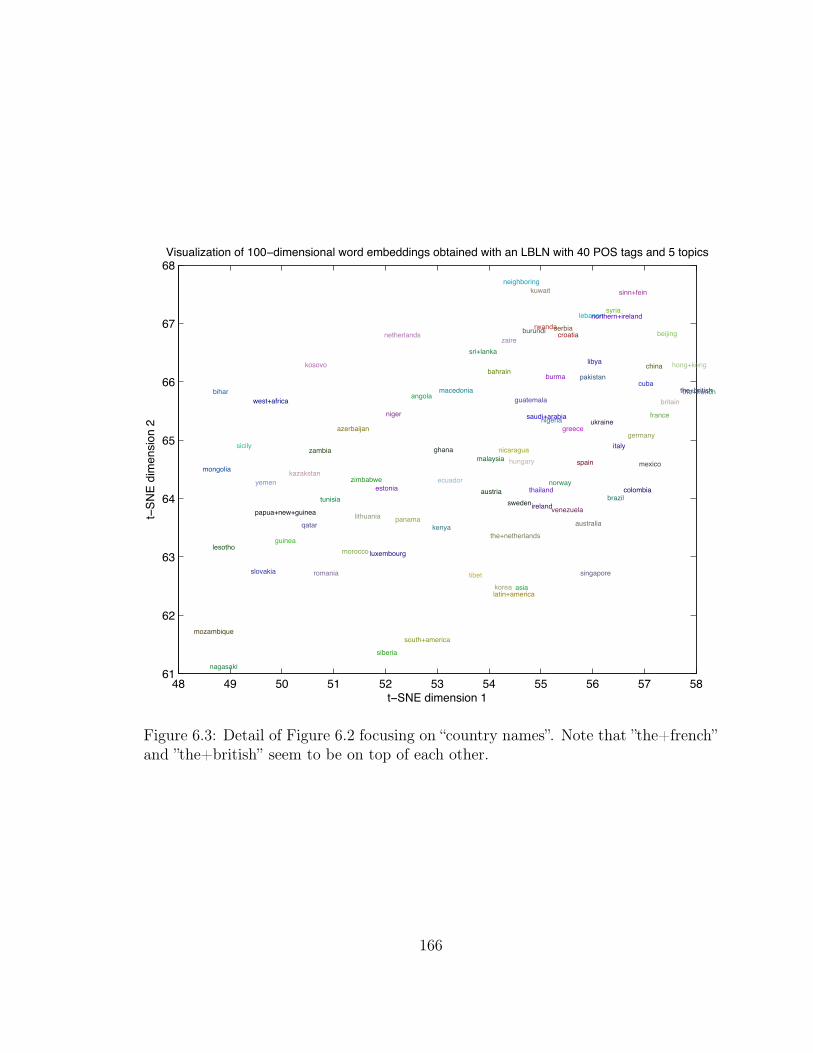
48 49 50 51 52 53 54 55 56 57 5861

62

63

64

65

66

67

68

niger

macedonia

ecuador

zaire

spain

kosovo

kenya

tunisia

malaysiaghana

luxembourg

nigeria

australia

bihar

rwanda

the+netherlandsguinea

sweden

azerbaijan

kazakstan

lebanon

hungary

venezuela

saudi+arabia

mexico

bahrain

netherlands

china

norway

greece

yemen

burundi

nicaraguazambia

serbia

sicily

syria

korea

sri+lanka

cuba

austria

northern+ireland

ukraine

thailand

mozambique

ireland

latin+america

neighboring

estonia

guatemalawest+africa

romania

panama

kuwait

angola

south+america

brazil

britain

papua+new+guinea

hong+kong

zimbabwe

nagasaki

lithuania

sinn+fein

tibet

qatar

morocco

libya

pakistan

the+french

siberia

the+british

lesotho

asia

beijing

germany

burma

slovakia

france

italy

singapore

mongolia

croatia

colombia


t−SNE dimension 1

t−SN

E di

men

sion

2


Figure 6.3: Detail of Figure 6.2 focusing on “country names”. Note that ”the+french”and ”the+british” seem to be on top of each other.

166

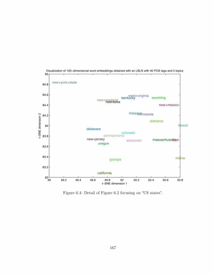
49 49.2 49.4 49.6 49.8 50 50.2 50.4 50.6 50.883

83.2

83.4

83.6

83.8

84

84.2

84.4

84.6

84.8

85

massachusettspennsylvania

missouri

wisconsin

minnesota

nebraska

hawaii

kentucky

new+york+state

california

utahnew+jersey

colorado

oregon

west+virginia

georgia

new+england

maine

wyoming

delaware

new+mexico

alabama


t−SNE dimension 1

t−SN

E di

men

sion

2


Figure 6.4: Detail of Figure 6.2 focusing on “US states”.

167

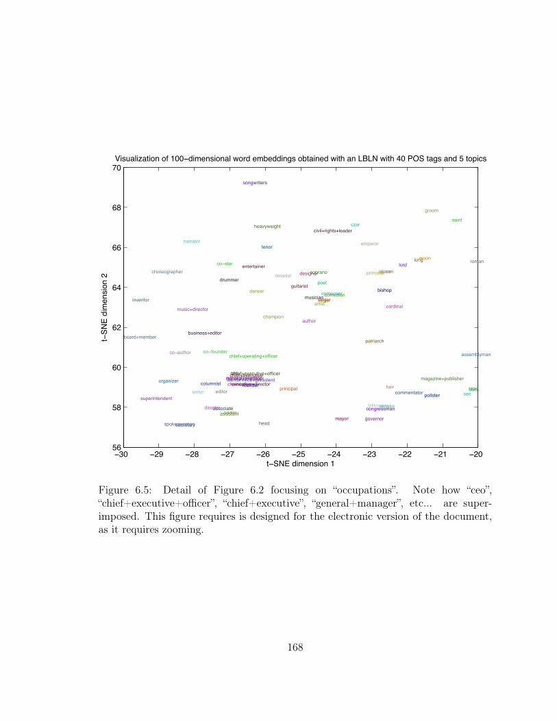
−30 −29 −28 −27 −26 −25 −24 −23 −22 −21 −2056

58

60

62

64

66

68

70

actor

moon

assemblyman

managing+editor

co−author

secretary

billionaire

composer

prince

assistantmayor

founder

music+director

tenor

artist

spokeswoman

dancer

owner

organizer magazine+publisher

designer

writer

guitarist

co−star

author

entertainerking

heir

cardinal

roman

bishop

princess

patriarch

songwriters

heavyweight

chairwoman

champion

columnist

poet

singer

chief+operating+officer

novelist

associatedirector

musician

czar

governor

ceo

executive+director

drummer

congressman

queen

co−founder

reps

chief+executive+officer

senator

chief+executive

comedian

pollster

groom

superintendent

sopranochoreographer

sen

head

inventor

emperor

sens

narrator

editor

general+manager

saint

civil+rights+leader

senior+vice+president

lord

principalcommentator

board+memberbusiness+editor


t−SNE dimension 1

t−SN

E di

men

sion

2


Figure 6.5: Detail of Figure 6.2 focusing on “occupations”. Note how “ceo”,“chief+executive+officer”, “chief+executive”, “general+manager”, etc... are super-imposed. This figure requires is designed for the electronic version of the document,as it requires zooming.

168

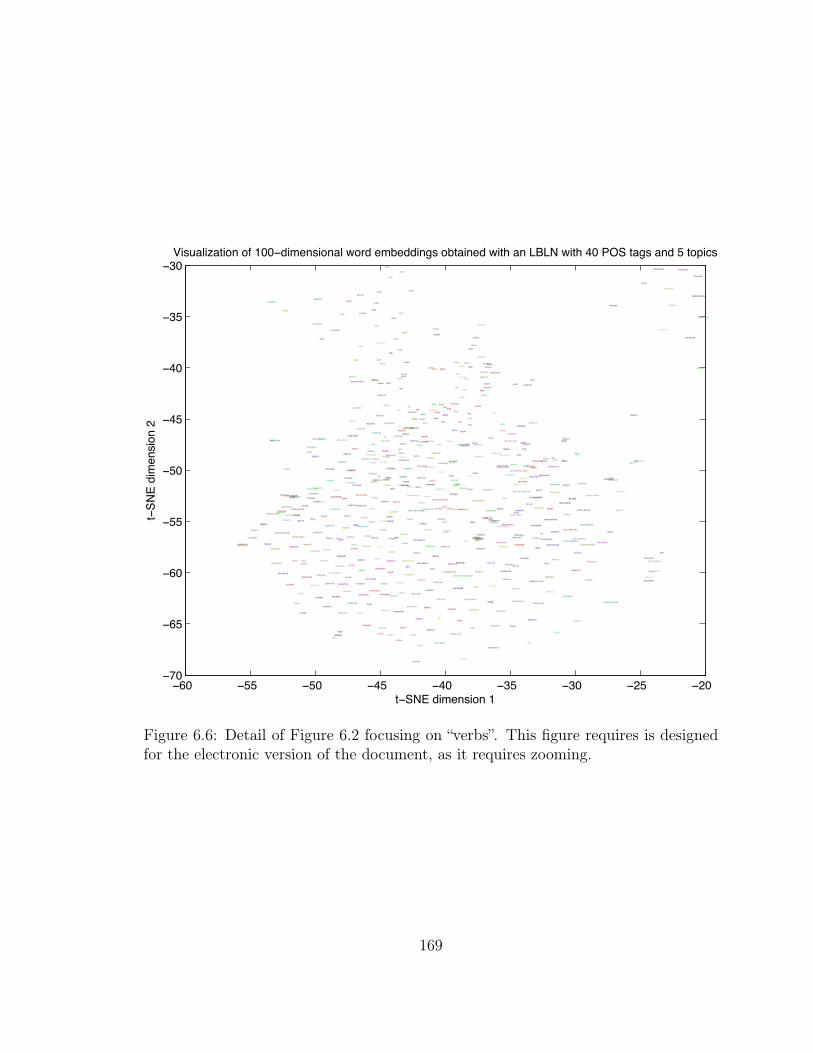
−60 −55 −50 −45 −40 −35 −30 −25 −20−70

−65

−60

−55

−50

−45

−40

−35

−30

come+oncome+in

check

satisfy

live+in

outlaw

steer

resign

stand+in

extract

testify

analyze

frenzied

travel+to

get+out

generate

drag

hamper

stay

threaten

sell

endanger

watch

cut+down

have+on

permit

pay+attention

add+up

spell+out

work

disband

manufacture

fill

relocate

contribute

take+effect

lackluster

weigh

spontaneous

harrowing

smash

complain

forget

deny

lockshovel

rewrite

detain

pay+off

turn+in

bring+in

boycott

discourageavert

refer

flush

indict

touch

waive

transform

revoke

file

remind

pity

streamline

am

destabilize

find+out

alter

fractured

show

get+off

persuade

root+out

fool

disagree+with

go+on

pinpoint

produce

pay+back

elaborate

interpret

thwart

bring+to

take+advantage

await

turn+to

back+down

feed

plead rule+out

speak+for

hinder

discuss

promote

sign+on

check+out

concentrate+on

enforce

squeeze

be+like

get+at

denotes

gain

find

hold+down

anticipate

penalize

emphasize

want

grab

shout

go+up

answer

overthrow

smell

look+for

erect

warntrim

tear

see

fly

backfire

interrupt

dig+out

secede

perform

abolish

end+up

shield

dig

broker

possess

share

define

oversee take+up

festive

put+downportray

hear

be+an

sing

illustrate

cut

ignite

bring+back

ward+off

figure+out

emerge

swallow

get+rid+of

hand+out

pretend

install

intervene

rein+in

believe+in

relate

express

assert put+together

absorb

keep+out

inspect

condemn

offset

come+down

stab

open+up

opt

pose

take+care

weakenmake+peace

take+off

connect

earn

offend

do+nothing

prop+up

boisterous

be+held

override

act+as

arrive

teach

violate

keep+up

clarify

turn+on

shine

distinguish

renounce

hold

soften

commutewrap

breathe

represent

pass

reopen

votequalify

realize

avenge

feel

bring

respond

turn+away

endure

interfere

hate

simplify provide+foraccuse

involve

speak

stand

wake+up

notify

take+control

do+in

stall

enlist

come+through

divide

exempt

reject

surround

get+away

distort

move+into

take+a+lookrecognize

shoot+down

resent

carry

dump

deal

’m

relieve

flourish

scare

tout

prolong

lose

end

defer

cast

deliver

begin

constitute

continue

defraud

turn+around

penetrate

go+in

appeal

vote+in

disappear

celebrate get+through

forgive

get+in

address

smuggle

work+out

equip

extend+to

move

be+on

disperse

drink

scramble

identify

mobilize

turn+back

sue

appreciate

divert

react

suggest

merge

sever

concede

walk+away

lie+in

dislodge

squash

build+up

examine

eliminate

play

bring+up

managesolve

answer+for

come

toughen

run+away

contain

get+to

climb

perceive

resolve

stand+for

refrain

regulate

cover+for

save

invite

detect

muzzle

knock

commemorate

throw

intricate

preside rebut

resort+to

muster

fear

eradicate

cope+with

spin

evade

go+down

enrich

dispose+of

belong+to

count+on

work+in

pay+out

shrink

bolster

have+sex

solicit

undercutallay

join

haul

shake

keep+in

undergo

run+into

tackle

bypass

float

come+forward

form

stem

monitor

adjust

provide

assemblereinstate

pick+up

thaw

guess

starve

expose

invoke

indicate

proceed

characterize

discover

insist

unite

devastate

comply

postpone

dial

abandon

abide+by

eat

step+up

work+at

care

recruit

curtail

enroll

make+sense

confront

run

stave+off

reimburse

coincide

keep

publicize

supervise

stay+on

encourage

deflect

forge

move+in

bash

crack+down

invade

mean

pre−empt

retaliate

stick

dominate

act+on

set+a

depend+on

turn+over

argue

reflect

get+on+with

delete

call+on

run+in

create

topple

minimize

lie

take+part

inherit

need

seem

allow+for

designate

pave

take+into+account

depart

accelerate

load

embrace

slow+down

come+home

disguise

reveal

determine

sway

put+out

come+together

contradict

repeat

adopt

consult

accomplish

erase

inspire

walk+out

cause

expand

split

look+like

low−key

regard

attract

symbolize

update

consolidate

lay+off

belong

stir

repair

prohibit

come+with

regain

account+for

love

amend

treat

reverse

sign

tell

submit

spark

skip

recommend

agree

heal

build

compel

explore

flee

pray

quirky

be+restoredbuild+on

summon

review

use

heed

uncover

come+back

change

legalize

crush

raise

contend get+together

leap

tighten

hide

injure

clean+up

differ

suppress

appease

boast

unveil

return

release

pay+for

feisty

fall+into

stand+by

snap

lure

nudge

show+up

compete

think+of

urge

coordinate

back+out

arise

retire

say

collect

manipulate

bolt

move+on

trace

cut+short

deduct

shoot

interact

beat

wrenching

deploy

attend

inject

donate

resemble

finish

go+backrun+forgo+out

bounce

claim

initiate

adhere

elect

conceal

handle

come+upremember

trap

sleep

forgo

buy+food

revive

ask

quit

recapture


t−SNE dimension 1

t−SN

E di

men

sion

2


Figure 6.6: Detail of Figure 6.2 focusing on “verbs”. This figure requires is designedfor the electronic version of the document, as it requires zooming.

169

Chapter 7

Conclusion

Parsifal - the kind of opera that starts at six

o’clock and after it has been going three

hours, you look at your watch and it says

6:20

David Randolph, conductor

Dear Reader, thank you for navigating through this extended account of my doc-

toral work. It introduced a new and simple methodology to modeling time series and

sequences, resorting to dynamics on hidden variable representations.

The major obstacle to overcome was the intractable problem of inferring latent rep-

resentations of sequences with (non)linear dynamics. Although numerous approaches

had been introduced in the past decade to solve that problem, consisting mostly of

variational Bayes and sampling methods, I proposed a simple maximum a posteriori

gradient-based inference enabled by a constant partition function, and a deterministic

Expectation-Maximization learning procedure. I justified that these approximations

were principled, and demonstrated the efficiency of my method on several real world

problems and datasets, where I achieved state-of-the-art results.

There are multiple reasons that explain why DFGs work so well with a MAP ap-

170

proximation of latent variables, even though the distribution of the latent variables

could theoretically be multimodal. These reasons differ from dataset to dataset. For

instance, most of the dataset that I considered, with the exception of the gene reg-

ulation data, were relatively long, dispensing with the need to model uncertainty in

the data, and thus well suited for energy-based methods. In the only case when the

dataset was very short (mRNA micro-arrays), I used heavily regularized simple linear

or nonlinear models. Secondly, I would always regularize the hidden representations

to limit their information content. Thirdly, I would in some cases initialize the hid-

den representations in an unsupervised way, using Singular Value Decomposition, to

further avoid suboptimal (local minima) solutions.

This multiple proof of principle demonstrated that a MAP inference was a valid

simplification, whose benefits were multiple: thanks to DFGs, one could learn long

sequences in linear time, handle high-dimensional hidden and observed variables, and

most importantly, model highly nonlinear dynamics and observation functions. As

I explained in Chapter 3, the computational complexity of DFGs is dominated by

the E-step inference, and it is linear in the number T of training samples, linear in

the number of observed variables and quadratic in the number of hidden variables.

More precisely, if we note |W| the number of parameters of the model, the total

computational complexity of one inference step over the full sequence is O (T |W|).

The DFG algorithm is therefore comparable, in terms of running time, to Back-

Propagation Through Time for Recurrent Neural Networks, but unlike the latter, it

explicitly optimizes the hidden representations.

Further investigations are envisioned, regarding the inference of gene regulation

networks and epileptic seizure prediction from EEG.

171

A word on the software implementation

The factor graph formulation makes our algorithm inherently modular and relatively

easy to implement as software1.

Each module needs only two functions to be defined, which we call fprop and

backprop. The fprop function is used to forward-propagate the variables through the

factor’s function and to evaluate the energy of the factor; the backprop function is used

to evaluate the derivatives of the loss of the factor with respect to both the function’s

parameters and the latent variables (if they serve as inputs to the function). For this

reason, any function and energy/loss that are differentiable can be used. The loss

function L consists in the sum of energies at each factor, plus regularization terms on

the latent variables and on the parameters of the module.

One then needs to define an E-step relaxation function that performs iterated fprop

and backprop on the latent variables until convergence, and several M-step functions,

one per type of factor/module. Both the E-step and M-step can consist in simple

gradient descents; the M-step can further benefit from other types of optimizations,

such as stochastic gradient (Bottou, 2004), exact solution to ridge regression, or

conjugate gradient (LeCun et al., 1998b).

Remaining portions of code deal with data pre-processing, early stopping strate-

gies and bookkeeping the energies and statistics on latent variables and parameters.

Although we ultimately made four different implementations of our software for

the four problems we handled, all the algorithms possessed the same properties enun-

ciated above. Two implementations are currently being used by other researchers,

respectively for the inference of gene regulation networks and for statistical lan-

guage modeling. A third software release is planned, concerning the Dynamic Auto-1Which we did in Lush (available at http://lush.sourceforge.net) and Matlab (by Mathworks).

172

Encoders, which could be applied not only to text but also other types of data, such

as features derived from EEG or perhaps even musical notation . . .

173

Bibliography

Abarbanel, H., Brown, R., Sidorowich, J. and Tsimring, L. (1993). The

analysis of observed chaotic data in physical systems. Reviews of Modern Physics

65.

Akaike, H. (1973). Information theory and an extension to the maximum likelihood

principle. In 2nd International Symposium on Information Theory .

Alvarez, M., Luengo, D. and Lawrence, N. (2009). Latent force models. In

ICML.

Alvarez-Buylla, E., Benitez, M., Balleza-Davila, E., Chaos, A., Espinosa-

Soto, C. and Padilla-Longoria, P. (2007). Gene regulatory network models for

plant development. Current Opinion in Plant Biology 10, 83–91.

Angus, J., Beal, M., Li, J., Rangel, C. and Wild, D. (2010). Inferring tran-

scriptional networks using prior biological knowledge and constrained state-space

models. In M. R. Neil Lawrence, Mark Girolami and G. Sanguinetti, eds., Learn-

ing and Inference in Computational Systems Biology . Cambridge, MA: MIT Press,

pages 117–153.

174

Aristidou, A., Cameron, J. and Lasenby, J. (2008). Real-time estimation of

missing markers in human motion capture. In Proceedings of the 2nd International

Conference on Bioinformatics and Biomedical Engineering ICBBE’08 .

Arnhold, J., Grassberger, P., Lehnertz, K. and Elger, C. (1999). A robust

method for detecting interdependence: applications to intracranially recorded EEG.

Physica D 134, 419–430.

Aschenbrenner-Scheibe, R., Maiwald, T., Winterhalder, M., Voss, H. and

Timmer, J. (2003). How well can epileptic seizures be predicted? An evaluation

of a nonlinear method. Brain 126, 2616–2626.

Bakker, R., Schouten, J., Giles, C., Takens, F. and van den Bleek, C.

(2000). Learning chaotic attractors by neural networks. Neural Computation 12,

2355–2383.

Baldi, P. and Rosen-Zvi, M. (2005). On the relationship between deterministic

and probabilistic directed graphical models: From bayesian networks to recursive

neural networks. Neural Networks 18, 1080–1086.

Bangalore, S. (1997). Complexity of Lexical Descriptions and its Relevance to Par-

tial Parsing . Ph.D. thesis, University of Pennsylvania, Philadelphia, PA.

Bangalore, S. and Joshi, A. (1999). Supertagging: An approach to almost parsing.

Computational Linguistics 25.

Barber, D. (2003). Dynamic bayesian networks with deterministic latent tables.

In NIPS’03: Advances in Neural Information Processing Systems . Cambridge MA:

MIT Press.

175

Barenco, M., Tomescu, D., Brewer, D., Callard, R., Stark, J. and Hubank,

M. (2006). Ranked prediction of p53 targets using hidden variable dynamic mod-

eling. Genome Biology 7.

Beal, M., Falciani, F., Ghahramani, Z., Rangel, C. and Wild, D. (2005).

A bayesian approach to reconstructing genetic regulatory networks with hidden

factors. Bioinformatics 21, 349–356.

Bengio, Y., Ducharme, R., Vincent, P. and Jauvin, C. (2003). A neural

probabilistic language model. Journal of Machine Learning Research 3, 1137–1155.

Bengio, Y. and Frasconi, P. (1995). An input/output HMM architecture. In

G. Teusauro, D. Touretzky and T. Leen, eds., Advances in Neural Information

Processing Systems NIPS’94 . Cambridge, MA: Morgan Kaufmann, MIT Press.

Bengio, Y., Lamblin, P., Popovici, D. and Larochelle, H. (2006). Greedy

layer-wise training of deep belief networks. In NIPS .

Bengio, Y., Simard, P. and Frasconi, P. (1994). Learning long-term dependencies

with gradient descent is difficult. IEEE Transactions on Neural Networks 5, 157–

166.

Bishop, C. (2006). Pattern recognition and machine learning . New York, NY:

Springer.

Blei, D. and Lafferty, J. (2006). Dynamic topic models. In ICML.

Blei, D. and McAulife, J. (2007). Supervised topic models. In NIPS .

Blei, D., Ng, A. and Jordan, M. (2003). Latent dirichlet allocation. Journal of

Machine Learning Research 3, 993–1022.

176

Blitzer, J., Weinberger, K., Saul, L. and Pereira, F. (2004). Hierarchical

distributed representations for statistical language modeling. In Advances in Neural

Information Processing Systems .

Bonneau, R., Facciotti, M., Reiss, D., Schmid, A., Pan, M., Kaur, A.,

Thorsson, V., Shannon, P., Johnson, M., Bare, J. and et al (2007). A

predictive model for transcriptional control of physiology in a free living cell. Cell

131, 1354–1365.

Bonneau, R., Reiss, D., Shannon, P., Facciotti, M., Hood, L., Baliga, N.

and Thorsson, V. (2006). The inferelator: an algorithm for learning parsimonious

regulatory networks from systems-biology data sets de novo. Genome Biology 7.

Bottou, L. (2004). Stochastic learning. In U. v. L. O. Bousquet, ed., Advanced

Lectures on Machine Learning . Berlin: Springer Verlag, pages 146–168.

Box, G. and Jenkins, G. (1976). Time Series Analysis, Forecasting and Control .

Oakland, CA: Holden Day, 2nd edition edition.

Buntine, W. (2009). Estimating likelihoods for topic models. In Z.-H. Zhou and

T. Washio, eds., Advances in Machine Learning , volume 5828 of Lecture Notes in

Computer Science. Springer Berlin / Heidelberg, pages 51–64.

Casdagli, M. (1989). Nonlinear prediction of chaotic time series. Physica D 35,

335–356.

Chen, S. F. and Goodman, J. (1996). An empirical study of smoothing techniques

for language modeling. In Proceedings of the Thirty-Fourth Annual Meeting of

the Association for Computational Linguistics . San Francisco: Morgan Kaufmann

Publishers.

177

Chopra, S., Thampy, T., Leahy, J., Caplin, A. and LeCun, Y. (2007). Dis-

covering the hidden structure of house prices with a non-parametric latent manifold

model. In Knowledge Discovery and Data Mining .

Collobert, R. and Weston, J. (2008). A unified architecture for natural lan-

guage processing: deep neural networks with multitask learning. In ICML ’08:

Proceedings of the 25th international conference on Machine learning . ISBN 978-

1-60558-205-4.

Cortes, C. and Vapnik, V. (1995). Support vector networks. Machine Learning

20, 273–97.

Cybenko, G. (1989). Approximation by superpositions of a sigmoidal function.

Mathematics of Control, Signals and Systems 2, 303–314.

Davis, J. and Goadrich, M. (2006). The relationship between precision-recall and

roc curves. In ICML.

Debole, F. and Sebastiani, F. (2005). An analysis of the relative hardness of the

Reuters-21578 subsets. Journal of the American Society for Information Science

and Technology 56, 584–596.

Deerwester, S., Dumais, S., Furnas, G., Landauer, T. and Harshman, R.

(1990). Indexing by latent semantic analysis. Journal of the American Society for

Information Science 41, 391–407.

Dempster, A., Laird, N. and Rubin, D. (1977). Maximum likelihood from

incomplete data via the EM algorithm. Journal of the Royal Statistical Society B

39, 1–38.

178

Durrett, R. (1996). Stochastic Calculus: A Practical Introduction. Boca Raton, FL:

CRC Press.

Efron, B., Hastie, T., Johnstone, I. and R., T. (2004). Least angle regression.

Annals of Statistics 32, 407–499.

Gao, P., Honkela, A., Rattray, M. and Lawrence, N. (2008). Gaussian process

modeling of latent chemical species: applications to inferring transcription factor

activities. Bioinformatics 24, i70–i75.

Gehler, P., Holub, A. and Welling, M. (2006). The rate adapting poisson model

for information retrieval and object recognition. In ICML.

Ghahramani, Z. (1998). Learning Dynamic Bayesian Networks . Lecture Notes in

Artificial Intelligence. Berlin: Springer-Verlag, pages 168–197.

Ghahramani, Z. and Roweis, S. (1999). Learning nonlinear dynamical systems

using an em algorithm. In Advances in Neural Information Processing Systems

NIPS’99 . Cambridge, MA: Morgan Kaufmann, MIT Press.

Gidofalvi, G. and Elkan, C. (2003). Using news articles to predict stock price

movements. Technical report, Department of Computer Science and Engineering,

University of California, San Diego.

Girard, A., Rasmussen, C., Candela, J. and Murray-Smith, R. (2003). Gaus-

sian process priors with uncertain inputs - application to multiple-step ahead time

series forecasting. In Advances in Neural Information Processing Systems NIPS’03 .

Cambridge, MA: MIT Press.

179

Goffin, V., Allauzen, C., Bocchieri, E., Hakkani-Tur, D., Ljolje, A.,

Parthasarathy, S., Rahim, M., Riccardi, G. and Saraclar, M. (2005). The

AT&T WATSON Speech Recognizer. In Proceedings of ICASSP . Philadelphia, PA.

Griffiths, T. and Steyvers, M. (2004). Finding scientific topics. PNAS 10, 5228–

5235.

Griffiths, T., Steyvers, M., Blei, D. and Tenenbaum, J. (2005). Integrating

topics and syntax. In Advances in Neural Information Processing Systems .

Gutierrez, R., Gifford, M., Poultney, C., Wang, R., Shasha, D., Coruzzi,

G. and Crawford, N. (2007). Insights into the genomic nitrate response using

genetics and the sungear software system. Journal of Experimental Botanics 58,

2359–2367.

Herring, C. and Palmore, J. (1995). Random number generators are chaotic.

Communications of the ACM 38.

Hinton, G., Dayan, P., Frey, B. and Neal, R. (1995). The wake-sleep algorithm

for unsupervised neural networks. Science 268, 1158–1161.

Hinton, G., Osindero, S. and Teh, W.-H. (2006). A fast learning algorithm for

deep belief nets. Neural Computation 18, 1527–1554.

Hinton, G. and Salakhutdinov, R. (2006). Reducing the dimensionality of data

with neural networks. Science 313, 504–507.

Hirose, O., Yoshida, R., Imoto, S., Yamaguchi, R., Higuchi, T., Charnock-

Jones, D., Print, C. and Miyano, S. (2008). Statistical inference of transcrip-

tional module-based gene networks from time course gene expression profiles by

using state space models. Bioinformatics 24, 932–942.

180

Hochreiter, S. and Schmidhuber, J. (1995). Long short-term memory. Neural

Computation 9, 1735–1780.

Ilin, A., Valpola, H. and Oja, E. (2004). Nonlinear dynamical factor analysis for

state change detection. IEEE Transactions on Neural Networks 15, 559–575.

Jaeger, J. and Monk, N. (2010). Reverse engineering of gene regulatory networks.

In M. R. Neil Lawrence, Mark Girolami and G. Sanguinetti, eds., Learning and

Inference in Computational Systems Biology . Cambridge, MA: MIT Press, pages

9–35.

Jelinek, F. (2005). Some of my best friends are linguists. Language Resources and

Evaluation 39, 25–34. ISSN 1574-020X. 10.1007/s10579-005-2693-4.

Joachims, T. (1998). Text categorization with support vector machines: Learning

with many relevant features. In ECML.

Joshi, A. K. (1987). An introduction to tree adjoining grammars. In A. Manaster-

Ramer, ed., Mathematics of Language. Amsterdam: John Benjamins.

Kalman, R. E. (1960). A new approach to linear filtering and prediction problems.

Transaction of the ASME - Journal of Basic Engineering , 35–45.

Katz, S. (1987). Estimation of probabilities from sparse data for the language moel

component of a speech recognizer. IEEE Transactions on Acoustics, Speech and

Signal Processing ASSP-35, 400–401.

Keshamouni, V., Jagtap, P., Michailidis, G., Strahler, J. and Kuick, R.

(2009). Temporal quantitative proteomics by iTRAQ 2D-LC-MS/MS and cor-

responding mRNA expression analysis identify post-transcriptional modulation

181

of actin-cytoskeleton regulators during TGF-beta-induced epithelial-mesenchymal

transition. Journal of Proteome Research 8, 35–47.

Kim, M. and Pavlovic, V. (2007). Conditional state space models for discrimina-

tive motion estimation. In IEEE International Conference on Computer Vision.

Kohlmorgen, J., Muller, K.-R. and Pawelzik, K. (1994). Competing predictors

segment and identify switching dynamics. In P. M. M. Marinaro, ed., ICANN’94:

Proceedings of the International Conference on Artificial Neural Networks . London

Berlin Heidelberg: Springer.

Kohlmorgen, J., Muller, K.-R. and Pawelzik, K. (1998). Analysis of drifting

dynamics with neural network hidden markov models. In NIPS’97: Advances in

Neural Information Processing Systems . Cambridge, MA: MIT Press.

Kolenda, T. and Kai Hansen, L. (2000). Independent components in text. In

Advances in Independent Component Analysis .

Krogh, A., Thorbergsson, G. and Hertz, J. (1990). A cost function for internal

representation. In Advances in Neural Information Processing Systems .

Krouk, G., Crawford, N., Coruzzi, G. and Tsay, Y. (2010). Nitrate signaling:

adaptation to fluctuating environments. Current Opinion in Plant Biology .

Krouk, G., Mirowski, P., Yann, Y., Shasha, D. and Coruzzi, G. (Provi-

sionally accepted for publication). High-resolution dynamics of transcriptome re-

sponses to no3- in arabidopsis roots: Molecular physiology and predictive modeling.

Genome Biology .

Kschischang, F., Frey, B. and Loeliger, H.-A. (2001). Factor graphs and the

sum-product algorithm. IEEE Transactions on Information Theory 47, 498–519.

182

Kuo, J.-M. and Principe, J. (1994). Reconstructed dynamics and chaotic signal

modeling. In IEEE International Conference on Neural Networks .

Lafferty, J., McCallum, A. and Pereira, F. (2001). Conditional random fields:

Probabilistic models for segmenting and labeling sequence data. In Proceedints of

the International Conference on Machine Learning . San Francisco, CA: Morgan

Kaufmann.

Lahdesmaki, H., Shmulevich, I. and Yli-Harja, O. (2003). On learning gene

regulatory networks under the boolean network model. Machine Learning 52, 147–

167.

Lang, K. and Hinton, G. (1988). The development of the time-delay neural

network architecture for speech recognition. Technical Report CMU-CS-88-152,

Carnegie-Mellon University.

Lawrence, N. (2004). Gaussian process latent variable models for visualisation of

high dimensional data. In Advances in Neural Information Processing Systems

NIPS’04 . Cambridge, MA: MIT Press.

Lawrence, N. and Sanguinetti, G. (2007). Modelling trancriptional regulation

using gaussian processes. In NIPS .

Le Van Quyen, M., Foucher, J., Lachaux, J.-P., Rodriguez, E., Lutz, A.,

Martinerie, J. and Varela, F. (2001). Comparison of hilbert transform and

wavelet methods for the analysis of neuronal synchrony. Journal of Neuroscience

Methods 11, 83–98.

183

Le Van Quyen, M., Navarro, V., Martinerie, J., Baulac, M. and Varela, F.

(2003). Toward a neurodynamical understanding of ictogenesis. Epilepsia 44/12,

30–43.

LeCun, Y., Bottou, L., Bengio, Y. and Haffner, P. (1998a). Gradient-based

learning applied to document recognition. Proceedings of the IEEE 86, 2278–2324.

LeCun, Y., Bottou, L., Orr, G. and Muller, K. (1998b). Efficient backprop. In

K. M. G. Orr, ed., Neural Networks: Tricks of the trade, Lecture Notes in Computer

Science. Berlin/Heidelberg: Springer, pages 9–50.

LeCun, Y., Chopra, S., Hadsell, R. and Huang, F. (2006). A tutorial on

energy-based learning. In Predicting Structured Outputs . MIT Press.

Lendasse, A., Oja, E. and Simula, O. (2004). Times series prediction competi-

tion: The cats benchmark. In Proceedings of IEEE International Joint Conference

on Neural Networks (IJCNN), volume 2.

Levin, E. (1993). Hidden control neural architecture modeling of nonlinear time-

varying systems and its applications. IEEE Transactions on Neural Networks 4,

109–116.

Liu, G. and McMillan, L. (2006). Estimation of missing markers in human motion

capture. The Visual Computer 22, 721–728.

Lorenz, E. (1963). Deterministic nonperiodic flow. Journal of Atmospheric Sciences

20, 130–141.

Lozano, A., Abe, N., Liu, Y. and Rosset, S. (2009). Grouped graphical granger

modeling for gene expression regulatory networks discovery. Bioinformatics 25,

110–118.

184

MacKay, D. (2003). Information Theory, Inference and Learning . Cambridge, UK:

Cambridge University Press.

Maiwald, T., Winterhalder, M., Aschenbrenner-Scheibe, R., Voss, H. and

Schulze-Bonhage, A. (2004). Comparison of three nonlinear seizure prediction

methods by means of the seizure prediction characteristic. Physica D 194, 357–368.

Mallat, S. (1999). A Wavelet Tour of Signal Processing . San Diego, CA: Elsevier,

Academic Press.

Mattera, D. and Haykin, S. (1999). Support vector machines for dynamic recon-

struction of a chaotic system. In A. S. B. Scholkopf, C.J.C. Burges, ed., Advances

in Kernel Methods: Support Vector Learning . Cambridge, MA: MIT Press, pages

212–239.

Mirowski, P., Chopra, S., Balakrishnan, S. and Bangalore, S. (2010a).

Feature-rich continuous language models for speech recognition. In Proceedings

of the IEEE Workshop on Spoken Language Technology .

Mirowski, P., Chopra, S., Balakrishnan, S. and Bangalore, S. (2010b). Sys-

tem and method for feature-rich continuous space language models. US Patent

Application AT&T Docket 2010-0851.

Mirowski, P. and LeCun, Y. (2009). Dynamic factor graphs for time series mod-

eling. In European Conference on Machine Learning .

Mirowski, P., Madhavan, D. and LeCun, Y. (2007). Time-delay neural networks

and independent component analysis for eeg-based prediction of epileptic seizures

propagation. In AAAI .

185

Mirowski, P., Madhavan, D., LeCun, Y. and Kuzniecky, R. (2008). Compar-

ing svm and convolutional networks for epileptic seizure prediction from intracra-

nial eeg. In Proceedings of the IEEE Workshop on Machine Learning for Signal

Processing .

Mirowski, P., Madhavan, D., LeCun, Y. and Kuzniecky, R. (2009a). Clas-

sification of patterns of eeg synchronization for seizure prediction. Clinical Neuro-

physiology 120, 1927–1940.

Mirowski, P., Madhavan, D., LeCun, Y. and Kuzniecky, R. (2009b). Method,

system and computer-accessible medium for classification of at least one ictal state.

International Patent Publication WO 2009/149126 A2.

Mirowski, P., Ranzato, M. and LeCun, Y. (2010c). Dynamic auto-encoders for

semantic indexing. In Proceedings of the NIPS Deep Learning and Unsupervised

Learning Workshop.

Mnih, A. and Hinton, G. (2007). Three new graphical models for statistical

language modelling. In 24th International Conference on Machine Learning ICML.

ISBN 978-1-59593-793-3.

Mnih, A. and Hinton, G. (2008). A scalable hierarchical distributed language

model. In Advances in Neural Information Processing Systems NIPS .

Mnih, A., Zhang, Y. and Hinton, G. (2009). Improving a statistical language

model through non-linear prediction. Neurocomputing 72, 1414 – 1418. ISSN

0925-2312.

186

Moon, K. and Pavlovic, V. (2008). 3D human motion tracking using dynamic

probabilistic latent semantic analysis. In Canadian Conference on Computer and

Robot Vision CRV’08 .

Moon, T. (1996). The expectation-maximization algorithm. IEEE Signal Processing

Magazine 13, 47–60.

Morin, F. and Bengio, Y. (2005). Hierarchical probabilistic neural network lan-

guage model. In Advances in Neural Information Processing Systems NIPS .

Mukherjee, S., Osuna, E. and Girosi, F. (1997). Nonlinear prediction of chaotic

time series using support vector machines. In Proceedings of IEEE Workshop on

Neural Networks for Signal Processing NNSP’97 .

Muller, K., Smola, A., Ratsch, G., Scholkopf, B., Kohlmorgen, J. and

Vapnik, V. (1999). Using support vector machines for time-series prediction. In

A. J. S. B. Scholkopf, C. J. C. Burges, ed., Advances in Kernel Methods: Support

Vector Learning . Cambridge, MA: MIT Press, pages 212–239.

Murphy, K. and Mian, S. (1999). Modelling gene expression data using dynamic

bayesian networks. Technical report, Computer Science Division, University of

California and Life Sciences Division, Lawrence Berkeley National Laboratory.

Neal, R. and Hinton, G. (1998). A view of the em algorithm that justifies in-

cremental, sparse, and other variants. In M. Jordan, ed., Learning in Graphical

Models . Cambridge, MA: MIT Press, pages 355–370.

Nelson, L. and Stear, E. (1976). The simultaneous on-line estimation of parameters

and states in linear systems. IEEE Transactions on Automatic Control 21, 94–98.

187

Olshausen, B. and Field, D. (1997). Sparse coding with an overcomplete basis

set: a strategy employed by V1? Vision Research 37, 3311–3325.

Pavlovic, V., Frey, B. and Huang, T. (1999). Time-series classification us-

ing mixed-state dynamic bayesian networks. In Proceedings of the Conference on

Computer Vision and Pattern Recognition CVPR’99 , volume 2. IEEE Computer

Society.

Pruteanu-Malinici, I., Ren, L., Pailsey, J., Wang, E. and Carin, L. (2010).

Hierarchical bayesian modeling of topics in time-stamped documents. IEEE Trans-

actions on Pattern Analysis and Machine Intelligence 32, 996–1011.

Puskorius, G. and Feldkamp, L. (1994). Neurocontrol of nonlinear dynamical sys-

tems with kalman filter trained recurrent networks. IEEE Transactions on Neural

Networks 5, 279–297.

Rabiner, L. (1989). A tutorial on hidden markov models and selected applications

in speech recognition. Proceedings of the IEEE 77, 257–286.

Rangel, C., Angus, J., Ghahramani, Z., Lioumi, M., Sotheran, E., Gaiba,

A., Wild, D. and Falciani, F. (2004). Modeling t-cell activation using gene

expression profiling and state-space models. Bioinformatics 20, 1361–1372.

Ranzato, M. (2009). Unsupervised Learning of Feature Hierarchies . Ph.D. thesis,

Courant Institute of Mathematical Sciences, New York University.

Ranzato, M., Boureau, Y. and LeCun, Y. (2007). Sparse feature learning for

deep belief networks. In NIPS .

Ranzato, M. and Szummer, M. (2008). Semi-supervised learning of compact

document representations with deep networks. In ICML.

188

Resnik, P. (1999). Semantic similarity in a taxonomy: An information-based mea-

sure and its application to problems of ambiguity in natural language. Journal of

Artificial Intelligence Research 11, 95–130.

Robertson, C., Geva, S. and Wolff, R. (2007). News aware volatility forecast-

ing: Is the content of the news important? In Sixth Australasian Data Mining

Conference.

Rohwer, R. (1989). The moving targets training algorithm. Neural Networks 412,

100–109.

Rumelhart, D., Hinton, G. and Williams, R. (1986). Learning representations

by back-propagating errors. Nature 323, 533–536.

Salakhutdinov, R. and Hinton, G. (2007). Semantic hashing. In ACM SIGIR

Workshop on Information Retrieval and Applications of Graphical Models .

Salakhutdinov, R. and Hinton, G. (2009). Replicated softmax. In ICML.

Sarikaya, R., Emami, A., Afify, M. and Ramabhadran, B. (2010). Contin-

uous space language modeling technique. In IEEE International Conference on

Acoustics, Speech and Speech Processing ICASSP .

Sarkka, S., Vehtari, A. and Lampinen, J. (2004). Time series prediction by

kalman smoother with cross-validated noise density. In Proceedings of IEEE Inter-

national Joint Conference on Neural Networks (IJCNN), volume 2.

Schelter, B., Winterhalder, M., Maiwald, T., Brandt, A. and Schad, A.

(2006a). Do false predictions of seizures depend on the state of vigilance? a report

from two seizure-prediction methods and proposed remedies. Epilepsia 47, 2058–

2070.

189

Schelter, B., Winterhalder, M., Maiwald, T., Brandt, A. and Schad, A.

(2006b). Testing statistical significance of multivariate time series analysis tech-

niques for epileptic seizure prediction. Chaos 16.

Schulze-Bonhage, A., Kurth, C., Carius, A., Steinhoff, B. and Mayer, T.

(2006). Seizure anticipation by patients with focal and generalized epilepsy: a

multicentre assessment of premonitory symptoms. Epilepsy Research 70, 83–88.

Schwenk, H. (2010). Continuous-space language models for statistical machine

translation. The Prague Bulletin of Mathematical Linguistics 93, 137–146.

Schwenk, H. and Gauvain, J.-L. (2003). Using continuous space language models

for conversational speech recognition. In IEEE Workshop on Spontaneous Speech

Processing and Recognition SSPR.

Segal, E., Shapira, M., Regev, A., Pe’er, D., Botstein, D., Koller, D. and

Friedman, N. (2003). Module networks: identifying regulatory modules and their

condition-specific regulators from gene expression data. Nature Genetics 34, 166–

176.

Shimamura, T., Imoto, S., Yamaguchi, R., Fujita, A., Nagasaki, M. and

Miyano, S. (2009). Recursive regularization for inferring gene networks from

time-course gene expression profiles. BMC Systems Biology 3.

Spellman, P., Sherlock, G., Zhang, M., Iyer, V., Anders, K., Eisen, M.,

Brown, P., Botstein, D. and Futcher, B. (1998). Comprehensive identification

of cell cycle-regulated genes of the yeast saccharomyces cerevisiae by microarray

hybridization. Molecular Biology of the Cell 9, 3273–3297.

190

Stolcke, A. (2002). Srilm - an extensible language modeling toolkit. In 7th Interna-

tional Conference on Spoken Language Processing ICSLP .

Strogatz, S. (1994). Nonlinear Dynamics and Chaos. With Applications to Physics,

Biology, Chemistry, and Engineering . Studies in Nonlinearity. Westview Books,

Perseus Books Publishing, Cambridge, MA.

Sutskever, I. and Hinton, G. (2006). Learning multilevel distributed representa-

tions for high-dimensional sequences. In NIPS’06: Advances in Neural Information

Processing Systems . Cambridge, MA: Morgan Kaufmann, MIT Press.

Takens, F. (1981). Detecting strange attractors in turbulence, volume 898 of Lecture

Notes in Mathematics . Warwick, UK: Springer, pages 336–381.

Taleb, N. (2007). The Black Swan: The Impact of the Highly Improbable. New York,

NY: Random House.

Taylor, G., Hinton, G. and Roweis, S. (2006). Modeling human motion using

binary latent variables. In NIPS’06: Advances in Neural Information Processing

Systems . Cambridge, MA: Morgan Kaufmann, MIT Press.

Tibshirani, R. (1996). Regression shrinkage and selection via the lasso. Journal of

the Royal Statistics Society B 58, 267–288.

Tsay, R. (2005). Analysis of Financial Time Series . Wiley Series in Probability and

Statistics. Hoboken, NJ: John Wiley and Sons, second edition edition.

Van der Maaten, L. and Hinton, G. (2008). Visualizing data using t-SNE. JMLR

9.

Wahde, M. and Hertz, J. (2001). Modeling genetic regulatory dynamic in neural

development. Journal of Computational Biology 8, 429–442.

191

Waibel, A., Hanazawa, T., Hinton, G., Shikano, K. and Lang, K. (1989).

Phoneme recognition using time-delay neural networks. IEEE Transactions in Ac-

coustics, Speech, Signal Processing 37, 328–339.

Wan, E. (1993). Time series prediction by using a connectionist network with internal

delay lines. In N. A. G. A. S. Weigend, ed., Time Series Prediction: Forecasting the

Future and Understanding the Past . Reading, MA: Addison-Wesley, pages 195–217.

Wan, E. and Nelson, A. (1996). Dual kalman filtering methods for nonlinear pre-

diction, estimation, and smoothing. In Advances in Neural Information Processing

Systems , volume 9. Cambridge, MA: Morgan Kaufmann, MIT Press.

Wan, E. and Van Der Merwe, R. (2000). The unscented kalman filter for nonlin-

ear estimation. In Proceedings of the IEEE 2000 Symposium on Adaptive Systems

for Signal Processing, Communications, and Control AS-SPCC .

Wang, J., Fleet, D. and Hertzmann, A. (2006a). Gaussian process dynamical

models. In Advances in Neural Information Processing Systems NIPS’06 . Cam-

bridge, MA: MIT Press.

Wang, R., Guegler, K., LaBrie, S. and Crawford, N. (2000). Genomic analysis

of a nutrient response in Arabidopsis reveals diverse expression patterns and novel

metabolic and potential regulatory genes induced by nitrate. Plant Cell 12, 1491–

1510.

Wang, X. and McCallum, A. (2006). Topics over time: A non-markov continuous-

time model of topical trends. In KDD .

192

Wang, Y., Joshi, T., Zhang, X.-S., Xu, D. and Chen, L. (2006b). Inferring

gene regulatory networks from multiple microarray datasets. Bioinformatics 22,

2413–2420.

Weigend, A. and Gershenfeld, N. (1994). Time series prediction: Forecasting

the future and understanding the past . Reading, MA: Addison-Wesley.

Wierstra, D., Gomez, F. and Schmidhuber, J. (2005). Modeling systems with

internal state using evolino. In Proceedings of the 2005 Conference on Genetic and

Evolutionary Computation.

Williams, C. and Rasmussen, C. (1996). Gaussian processes for regression. In

Advances in Neural Information Processing Systems NIPS’96 . Cambridge, MA:

MIT Press.

Williams, R. and Zipser, D. (1995). Gradient-Based Learning Algorithms for

Recurrent Networks and Their Computational Complexity . Lawrence Erlbaum As-

sociates, pages 433–486.

Yamaguchi, R., Imoto, S. and Satoru, M. (2010). Network-based predictions

and simulations by biological state space models for drug mode of action. Journal

of Computer Science and Technology 25, 131–153.

Yamaguchi, R., Yoshida, R. and Imoto, S. (2007). Finding module-based gene

networks with state-space models. IEEE Signal Processing Magazine 37.

Yang, D. and Zhang, Q. (2000). Drift independent volatility estimation based on

high, low, open and close prices. Journal of Business 73, 477–491.

193

Zhang, Y., Hatch, K., Bacon, J. and Wernisch, L. (2010). An integrated

machine learning approach for predicting dosr-regulated genes in mycobacterium

tuberculosis. BMC Systems Biology 4.

Zou, H. and Hastie, T. (2005). Regularization and variable selection via the elastic

net. Journal of Royal Statistical Society B 67, 301–320.

194