HAL Id: hal-03609720 https://hal.archives-ouvertes.fr/hal-03609720 Submitted on 15 Mar 2022 HAL is a multi-disciplinary open access archive for the deposit and dissemination of sci- entific research documents, whether they are pub- lished or not. The documents may come from teaching and research institutions in France or abroad, or from public or private research centers. L’archive ouverte pluridisciplinaire HAL, est destinée au dépôt et à la diffusion de documents scientifiques de niveau recherche, publiés ou non, émanant des établissements d’enseignement et de recherche français ou étrangers, des laboratoires publics ou privés. Copyright Time Series Data in the ESPON Database Martin Charlton, Chris Brunsdon, Conor Cahalane, Lars Pforte To cite this version: Martin Charlton, Chris Brunsdon, Conor Cahalane, Lars Pforte. Time Series Data in the ESPON Database. [Research Report] ESPON. 2015. hal-03609720

Welcome message from author
This document is posted to help you gain knowledge. Please leave a comment to let me know what you think about it! Share it to your friends and learn new things together.
Transcript
HAL Id: hal-03609720https://hal.archives-ouvertes.fr/hal-03609720
Submitted on 15 Mar 2022
HAL is a multi-disciplinary open accessarchive for the deposit and dissemination of sci-entific research documents, whether they are pub-lished or not. The documents may come fromteaching and research institutions in France orabroad, or from public or private research centers.
L’archive ouverte pluridisciplinaire HAL, estdestinée au dépôt et à la diffusion de documentsscientifiques de niveau recherche, publiés ou non,émanant des établissements d’enseignement et derecherche français ou étrangers, des laboratoirespublics ou privés.
Copyright
Time Series Data in the ESPON DatabaseMartin Charlton, Chris Brunsdon, Conor Cahalane, Lars Pforte
To cite this version:Martin Charlton, Chris Brunsdon, Conor Cahalane, Lars Pforte. Time Series Data in the ESPONDatabase. [Research Report] ESPON. 2015. �hal-03609720�

i
Time Series Data in the
ESPON Database
June 2014
CONTENT
Time series data form inputs to the ESPON
Database, at spatial scales including NUTS0,
NUTS1, NUTS2 and NUTS3. Series are often
incomplete at the lower levels in the NUTS
hierarchy. The task is to impute the missing
values, and ensure the spatial coherence of
the estimates.
A methodology is presented for data
imputation based on an autoregressive
model which is fitted to the existing data,
and used to impute the missing values,
using a Bayesian approach. The spatial
coherence of the results is also ensured.
The metholodgy has been implemented
using the R language, and tested on typical
short-run time series for NUTS0, NUTS1,
NUTS2 and NUTS3 regions.
R and JAGS code to operationalise the
methodology is presented in this report,
and a suitable workflow is outlined.

ii
LIST OF AUTHORS
Martin Charlton, National Centre for Geocomputation
Chris Brunsdon, National Centre for Geocomputation
Conor Cahalane, National Centre for Geocomputation
Lars Pforte, National Centre for Geocomputation
Contact
Address
National Centre for Geocomputation
National University of Ireland, Maynooth
Maynooth
County Kildare
IRELAND

iii
TABLE OF CONTENT
Section Title Page
1 Introduction
1
2 ESPON Time Series
2
3 Missing data imputation
11
4 Implementation
21
5 ESPON time series in practice 37
Appendix
1 NUTS0 time series plots
42
2 Main analysis and imputation R functions
49
3 Core imputation function
67
4 JAGS code for MCMC (multiple NAs)
70
5 JAGS code for MCMC (single NA)
72
6 Missing data at NUTS0/1/2
74
7 Missing data heatmaps
77
8 Coherence constraint output 112
1
1. Introduction
A time series is a collection of observations made sequentially in time1. Time series are frequently encountered in (i) economics [Beveridge annual wheat
price series], (ii) physical sciences [monthly average air temperature] (iii) marketing [monthly product sales] (iv) demography [annual population
estimates] and (v) process control [weights of manufactured product sampled hourly] (vi) communication [binary series are common]. While many series are
usually measured at regular intervals (e.g.: year, month, week, day, hour, minute), there are series which occur irregularly, for example, major railway disasters, which are known as point processes. Time series analysis is
concerned with (i) description of the main properties of the series, (ii) explanation of the relationship between two series taken at the same time
[monthly atmospheric temperature readings, monthly measurements of the North Atlantic Oscillation] and (iii) prediction of (usually) future values.
Time series description can take several forms, but are intended to reveal the underlying structure of the series. This structure can include several
components2: Trend: an increase or decrease in the value of the series over time
Seasonality: a regular pattern of high and low values related to calendar time Long term cycles: periodicity not related to seasonality
Outliers: values which are unusually high or low in comparison with the rest of the data Abrupt changes: changes to the variation in the series or level
Variance: this may be constant over time or increase/decrease
Sources of data for ESPON series
Many of the tables required can be obtained from EUROSTAT. However, there
are much missing data. Depending on the series, the series may be complete to NUTS 3 back to 2000. For earlier years, data may only be available to NUTS2
level. This requires recourse to other sources, for which the most authoritative would be those from the National Statistical Offices (for example: Turkstat, Croatian Bureau of Statistics, Statistics Norway, and Statistische Ämter des
Bundes und der Länder). There are other sources, such as the OECD, and the EUROSTAT NewCronos database may be of assistance in completing the time
series.
1 Chatfield, C, 1989, The Analysis of Time Series, 4th edn, London: Chapman and Hall, p1 2 Shumway RH and Stoffer DS, 2010, Times Series Analysis and its Applications, 3rd edn,
New York: Springer

2
2. ESPON Time Series
The character of ESPON Series
The socio-economic time series which appear to be commonly encountered in the ESPON programme are annual counts or ratios for a restricted time period
(1990-2013)3. This implies that the longest series are less than 25 years, and some are far shorter. Missing data in the middle of a series shorten it still
further. Hyndman has reported in the effects of attempting to fit models to short series4. In 95 short economic series about 1/3 were random walks (they had no
structure). The series are also presented for the spatial units in the NUTS classification5, The
NUTS system is a hierarchical system for dividing up the economic territory of the EU for the purposes of the collection o regional statistics, socio-economic
analyses and framing EU regional policies. We are concerned mainly with the first 4 levels of the NUTS hierarchy, Tables of the NUTS regions and their codes, and correspondence tables for region adjustments are available from EUROSTAT.
The input and outputs from the ESPON database are in the form of rectangular files, as a Excel spreadsheets – each line of data is preceded by its NUTS code.
Some sheets, and the EUROSTAT tables present the NUTS codes of every unit in a single column (for example demo_r_gind3), which gives the impression of flattening the hierarchy, The key to the strategy for handling the time series is
to think of the cross-sectional structure at each time period, implied by the NUTS codes, explicitly as a tree. We shall return to this later.
The datasets in EUROSTAT and from other sources are often incomplete for the time periods and spatial scales of interest. There might be many reasons –
population censuses may only be carried out on a decadal basis. While national or regional intercensal population estimates may be provided by the national
agencies, data at lower level is less common. In the case of the RIATE example dataset, the pattern of missing data relative to
the lvarious levels in the NUTS hierarchy is: Complete
NUTSlevel NotOK OK
0 3 31
1 35 80
2 113 204
3 1239 222
3 Commission Regulation 11/2008 specifies the required time series starting years for
NUTS levels in 17 statistical domains. The domain Demography has a start year for 1990
for both NUTS2 and NUTS3. 4 Hyndman R, 2014, Fitting models to short time series,
URL:rob.hyndman.com/hindsight/short-time-series 5 http://epp.eurostat.ec.europa.eu/portal/page/portal/nuts_nomenclature/introduction

3
An entry in the NotOK column means that data for one or more time periods in the series was missing. The pattern was what proportion of data was missing by
NUTS level is below: NumberIncomplete
NUTSlevel 0 1 2 4 5 6 7 8 9 10 11 12 13 14 15 16 17 21 22
0 31 0 0 1 0 0 0 0 0 0 0 0 0 0 0 1 0 1 0
1 80 7 3 0 0 1 0 0 0 0 2 0 0 0 0 12 0 4 6
2 204 16 15 0 5 4 2 0 0 0 4 0 15 17 0 26 5 3 1
3 222 113 42 0 0 417 18 44 105 132 108 100 32 0 10 88 30 0 0
While most NUTS0 series are complete, 1 is missing four time periods, 1 is
missing 16, and one is missing 21! The situation deteriorates as we progress down the hierarchy, but this is to be expected. About 25% of the NUTS1 series are missing a substantial portion of their data (over 72% of each series are
missing). At NUTS1 and NUTS2 data is either mostly present or missing to a serious degree.
AT NUTS3 level, the modal group represents 6 missing entries and a moderate
number of regions have over 75% of their series missing.
This provides a challenge for the analyst. What should be done about the missing data? In survey analysis a common strategy is to analyses only those cases with complete data for the variables of interest. This raises the question as
to whether the mechanism for creating the missing variables is a random process. If it is not, then the possibility of introducing bias into the analysis
becomes a problem. With time series the problem is magnified: if a single value is missing from the series, should the analyst remove this series from the analysis, or should some attempt be made to complete the data?
0 3 6 9 12 16 20
NUTS0
05
10
20
30
0 3 6 9 12 16 20
NUTS1
020
40
60
80
0 3 6 9 12 16 20
NUTS2
050
100
150
200
0 3 6 9 12 16 20
NUTS3
0100
200
300
400

4
IBM's SPSS software offers several alternatives to allow the analyst to replace missing observations with an estimate. These include6
The mean of the series
The mean of nearby observations
The median of nearby observations
Linear interpolation
Linear trend using the time series index as a regressor
The mean of the series might be a unwise choice, particular if the series has a
rising trend, and the missing observation is at the beginning of the series. Approaches to linear interpolation are described in detail below. Linear trend may or may not be helpful, although if the residuals either side of the trend line
are all positive or negative, then the estimated value my be some distance from a desirable value.
Enders7 notes that the analyst should make the distinction between the missing data pattern and the missing data mechanism. He notes that the pattern
relates to the configuration of observed and unobserved data, whereas the mechanism permits a description of the relationship between the two in terms of
probability. Rubin8 proposed classified missing data mechamisms into three types: (1) missing at random, (2) missing completely at random and (3) missing not at random. MAR arises when the probability of missing data is related to the
values of some other measured variable in the dataset. MCAR arises when the the probability is unrelated to any other variable in the dataset – Elders uses the
adjective haphazard for this. MNAR arises when the probability of missing data on a variable is related to the values of the variable itself. Elders uses an example of cancer patients in a trial becoming so ill they are unable to continue
participation in the trial. The ESPON time series missing data are likely to arise from an MCAR process – they are certainly not MNAR (the population values are
too small to collect). However, they may be too expensive to collect.
Traditional methods for missing data
Expedient methods for dealing with missing data include deletion of the
observations with missing data. Listwise deletion, or complete case analysis, removes any observation with one or more missing values. A variant, pairwise deletion, or available-case analysis, removes variables on an analysis-by-
analysis case. This would result in the correlations in a correlation matrix potentially being based on different numbers of underlying observations.
Other expedient methods include imputation. Amongst these are replacement by the arithmetic mean, replacement by median, regression imputation, (and
stochastic regression imputation which adds a random number from the distribution of residuals), hot-deck imputation (scores are taken from similar
6
http://pic.dhe.ibm.com/infocenter/spssstat/v21r0m0/index.jsp?topic=%2Fcom.ibm.spss.
statistics.help%2Fidh_rmvx.htm 7 Enders, CK, 2010, Applied Missing Data Analysis, New York: Guilford Press 8 Rubin, DB, 1976, Inference and Missing Data, Biometrika, 63(3), 581-592

5
respondents answers), and last observation carried forward (a variant of this is described below).
Missing observations
An appropriate example is given by the M4D table M4Dpoptot1990-2011_20120522.xls. This contains estimates of residential population, and is
available at NUTS0, NUTS2, NUTS2 and NUTS3, from 1990 to 2012. The metadata in table 1 shows that the sources of data include EUROSTAT and the
national statistical agencies. However, in many cases data have not being available from these sources and has been imputed by the team at RIATE. The metadata reveals that 52 separate imputation approaches can be identified,
although these are variations on the same underlying imputation process.
Table 1: extracr from metadata in M4Dpoptot1990-2011_20120522.xls
ID Label Provider
1 1 Eurostat
2 1a Eurostat
3 1*a Eurostat, NewCronos database
4 1*b Eurostat, NewCronos database
5 2a ESPON M4D
6 3a Turkstat
7 4a Croatian Bureau of Statistics
8 4b Croatian Bureau of Statistics
9 4c Croatian Bureau of Statistics
10 6a GUS (Central Statistical Office of Poland)
11 10 Statistics Norway
12 11 Statistics Sweden
13 12 Statistische Ämter des Bundes und der Länder
14 13 Statistics Denmark
15 14 Statistics Portugal
16 15 Statistics Netherlands
17 16 Latvijas Statistika
18 17 Statistics Lithuania
19 18 Fürstentum Liechtenstein
20 20 Statistics Iceland
21 21 Instituto Nacional de Estadistica
22 22 Czech Statistical Office
23 23 Office Fédéral de la Statistique Suisse
24 24 Statistics Estonia
25 25 Statistics Finland
26 26 INSEE (Institut National de la Statistique et des Etudes Economiques)
27 27 Hungarian Central Statistics Office
28 29a Statistics Belgium - Bestat
29 29b Statistics Belgium
30 31 Republic of Macedonia, Statistical

6
31 33 Hellenic Statistical Authority (ElStat)
32 34 UK National Statistics
33 E1b ESPON M4D
34 E2a ESPON M4D
35 E2b ESPON M4D
36 T1a ESPON M4D
37 T1b ESPON M4D
38 SE1a ESPON M4D, New Cronos Database
39 SE1a* ESPON M4D, New Cronos Database
40 SE1b ESPON M4D, New Cronos Database
41 SE1c ESPON M4D, General Register Office for Scotland
42 SE1f ESPON M4D, Statistical Office of the Republic of Slovenia
43 SE1g ESPON M4D, Central Statistics Office Ireland
44 SE1h ESPON M4D, Statistics Iceland
45 SE1i ESPON M4D, Instituto Nacional de Estadistica
46 SE1j ESPON M4D, Republic of Macedonia State Statistical Office
47 SE1k ESPON M4D, UK National statistics
48 SE1l ESPON M4D, Istituto Nazionale di Statistica
49 SE1m ESPON M4D, Czech Statistical Office
50 SE1n ESPON M4D, Statistische Ämter des Bundes und der Länder
51 SE1o ESPON M4D, Office Fédéral de la Statistique Suisse
52 TE1b ESPON M4D
53 TE1c ESPON M4D
54 TE1d ESPON M4D
55 TE1e ESPON M4D
56 TE1f ESPON M4D
57 TE1g ESPON M4D
58 TE1h ESPON M4D
59 TE1i ESPON M4D
60 TE1j ESPON M4D
61 TE1k ESPON M4D
62 TE1l ESPON M4D
63 TE1m ESPON M4D
64 TE1n ESPON M4D
65 TE1o ESPON M4D
66 TE1p ESPON M4D
67 TE1q ESPON M4D
68 TE1r ESPON M4D
69 TE2a ESPON M4D
70 TE2b ESPON M4D
71 TE2c ESPON M4D
72 TE3a ESPON M4D
73 TE3b ESPON M4D
74 TE3c ESPON M4D

7
75 TE3d ESPON M4D
76 TE3e ESPON M4D
77 TE3f ESPON M4D
78 TE3g ESPON M4D
79 TE6a ESPON M4D
80 TE6b ESPON M4D
81 TE6c ESPON M4D
82 TE6d ESPON M4D
83 TE6e ESPON M4D
84 TE6f ESPON M4D
The RIATE team observed that data was more often missing for NUTS3 units
than NUTS 2, and more often NUTS2 than NUTS1. Their other observation was that data is either missing from the beginning of the series to an intermediate time period, or missing in a run in the middle of the series. That the NUTS
hierarchy provides a parent NUTSlevel-1 region for any groups of NUTSlevel regions lead them to an ingenious group of solutions based around LOCF. These boil
down essentially to two strategies. Let pt,r be the proportion of the parent NUTSlevel-1 region's population for NUTSlevel
region r in year t, and Nr is the number of NUTSlevel regions in a parent NUTSlevel-1 region. In any given year the following is true:
Nr
r
rtp1
, 1
Data missing from beginning of series
In the first case, which the RIATE team describe as retropolation, the data are
missing from 1990 to the time period last. The proportions are propagated backwards along the series from the earliest known value, plast+1,r.
lastt
pp rlastrt
...1990
,1,
The population estimates for the NUTSlevel regions are then obtained by
multiplying the appropriate NUTSlevel-1 population by the retropolated pt,r values.
Data missing from the middle of a series
In the second case, that of interpolation, the data are missing from time period first to time period last inclusive. This implies that the proportions are are known for time period first-1 and time period last+1. The intermediate proportions are
obtained by linear interpolation. If pfirst-1,r and plast-1,r are the known proportions of the time periods immediately adjacent to the run of missing observations,
then:

8
lastfirstt
firstlast
firsttppp rfirstrlastrt
...
2
1,1,1,
The population estimates for the NUTSlevel regions are then obtained by
multiplying the appropriate NUTSlevel-1 population by the interpolated pt,r values.
Data missing from the end of the series
In a case analogous to the first, values of the proportions can be propagated forward from the latest known pfirst-1,r to 2012 (or whatever is the last time period in the study) in an extrapolation:
2012...
,1,
firstt
pp rfirstrt
These imputations represent the application of an AR(0) time series model where the trend for the first and last case is zero, and linear in the interpolation
case. The imputed values will then exhibit the same behavioural characteristics of the parent series.
Partially missing data
In some cases, data is missing for a subset missing of the NUTSlevel regions. The proportions are then of the NUTSlevel-1 population less the sum of the non-missing NUTSlevel populations. If data is missing for only one region at NUTSlevel,
then we can regard it as embarrassingly estimatable, in that the missing values are obtained from the population for the NUTSlevel-1 region less the sum of the
non-missing NUTSlevel populations, without the need to bring the LOCF procedures into play.
Estimation and the NUTS hierarchy
The implementation of this approach implies that the estimation strategy is top-down. That is, as the proportions for NUTSlevel relative to NUTSlevel-1 are required, then the values at NUTSlevel-1 must be obtained first. Therefore, population
estimates at NUTS1 must be made first, relative to the NUTS0 values. Once these have been obtained, estimates at NUTS2 may be made, and finally,
estimates at NUTS3. The RIATE implementation was undertaken using Excel. Whilst this represents
activity and effort which might be regarded as heroic, it is almost impossible to debug, very difficult to check, and cannot be automated. For these reasons, it
cannot be recommended.
9
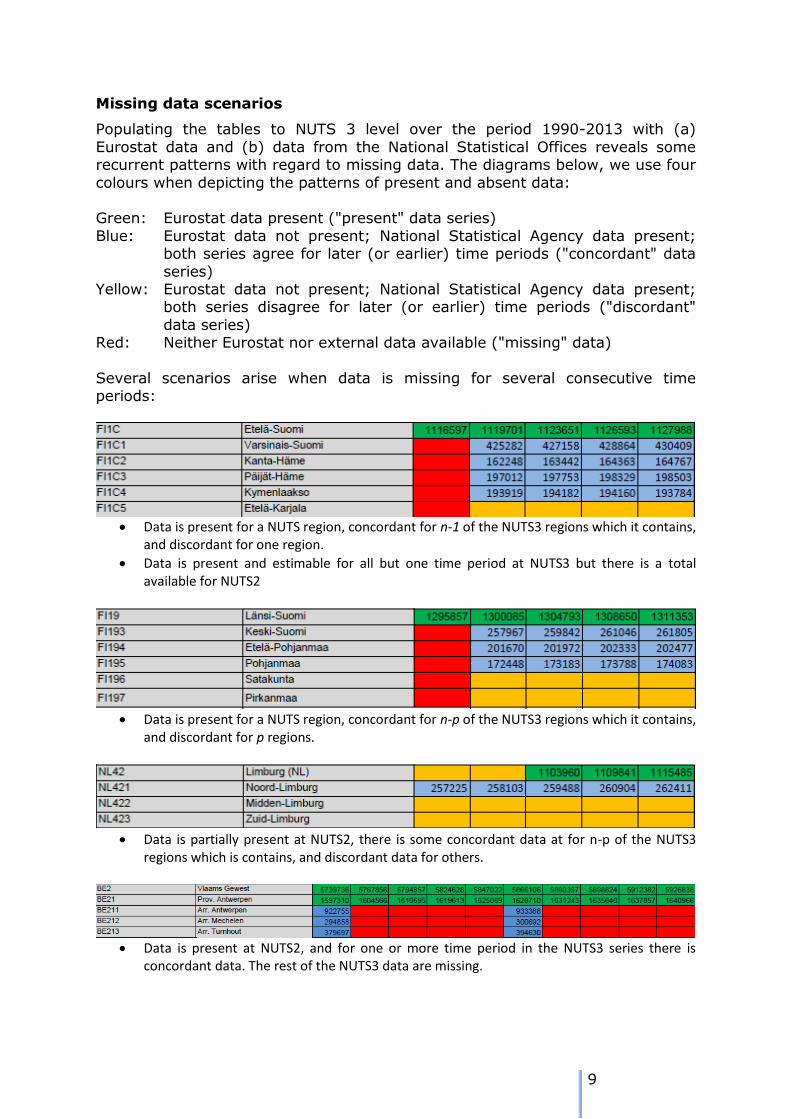
Missing data scenarios
Populating the tables to NUTS 3 level over the period 1990-2013 with (a)
Eurostat data and (b) data from the National Statistical Offices reveals some recurrent patterns with regard to missing data. The diagrams below, we use four
colours when depicting the patterns of present and absent data: Green: Eurostat data present ("present" data series)
Blue: Eurostat data not present; National Statistical Agency data present; both series agree for later (or earlier) time periods ("concordant" data
series) Yellow: Eurostat data not present; National Statistical Agency data present;
both series disagree for later (or earlier) time periods ("discordant"
data series) Red: Neither Eurostat nor external data available ("missing" data)
Several scenarios arise when data is missing for several consecutive time periods:
Data is present for a NUTS region, concordant for n-1 of the NUTS3 regions which it contains,
and discordant for one region.
Data is present and estimable for all but one time period at NUTS3 but there is a total available for NUTS2
Data is present for a NUTS region, concordant for n-p of the NUTS3 regions which it contains,
and discordant for p regions.
Data is partially present at NUTS2, there is some concordant data at for n-p of the NUTS3
regions which is contains, and discordant data for others.
Data is present at NUTS2, and for one or more time period in the NUTS3 series there is
concordant data. The rest of the NUTS3 data are missing.
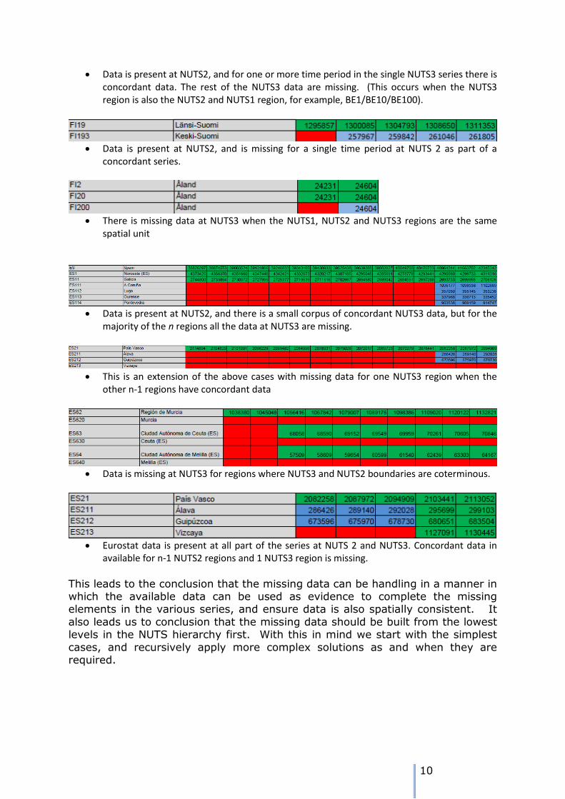
10
Data is present at NUTS2, and for one or more time period in the single NUTS3 series there is concordant data. The rest of the NUTS3 data are missing. (This occurs when the NUTS3 region is also the NUTS2 and NUTS1 region, for example, BE1/BE10/BE100).
Data is present at NUTS2, and is missing for a single time period at NUTS 2 as part of a
concordant series.
There is missing data at NUTS3 when the NUTS1, NUTS2 and NUTS3 regions are the same
spatial unit
Data is present at NUTS2, and there is a small corpus of concordant NUTS3 data, but for the
majority of the n regions all the data at NUTS3 are missing.
This is an extension of the above cases with missing data for one NUTS3 region when the
other n-1 regions have concordant data
Data is missing at NUTS3 for regions where NUTS3 and NUTS2 boundaries are coterminous.
Eurostat data is present at all part of the series at NUTS 2 and NUTS3. Concordant data in
available for n-1 NUTS2 regions and 1 NUTS3 region is missing.
This leads to the conclusion that the missing data can be handling in a manner in which the available data can be used as evidence to complete the missing elements in the various series, and ensure data is also spatially consistent. It
also leads us to conclusion that the missing data should be built from the lowest levels in the NUTS hierarchy first. With this in mind we start with the simplest
cases, and recursively apply more complex solutions as and when they are required.

11
3. Missing data imputation
Estimation
The scenarios suggest that we will require three components in the estimating strategy: (a) a suitable model for the existing data and (b) a means of ensuring
hierarchical spatial coherence in the series and (c) a means of representing the spatial hierarchy of the NUTS regions in each country
Experimentation of the existing ESPON series suggests that some relatively
simple models will yield reasonable results for the first component. Each series can be modelled with either a linear, quadratic or exponential trends, with an autocorrelated error term:
t
ta
t
t
tt
eeaP
tataaPt
taaP
1
0
2
210
10
where the error term is 0~N(0,) and t~N(t-1,) with t > 0 and ||<1.. The parameters a0, a1 and a2 are to be estimated. Both models can handle missing values – points for which no data is available – as well as provide forecasts,
backcasts and interpolation of missing data in the middle of a series. The generic term prediction covers these three eventualities.
Models for time series
To estimate data for a time series we need to start with a model. There are many such models in the time series analysis literature which may be applied. In
an autoregressive model the value of the series at time t depends on p previous values:
p
i
titit XcX1
By contrast in a moving average model, the error at time t depends on q
previous values:
q
j
jtjttX1
These can be combined to give an autoregressive moving average model:
q
j
jtj
p
i
ititt XcX11

12
Such models were given extensive treatment in Box and Jenkins (1970)9. They are conventionally fitted to a series which is stationary (that is, in which the
trend has been removed), a situation obtained by differencing. If the trend is
linear, the series might need to be differenced once (i.e. t = Xt – Xt-1); if the
trend is accelerating, second differences might be required. However, typically to obtain reliable estimates of the p autoregressive parameters and the q moving average parameters requires series of perhaps many 10s of
observations. We no have this luxury with the ESPON series.
Al alternative is to consider methods using Bayesian inference. We
conventionally model data D with some parameters using the probability
distribution P(D|); the might be the parameters from a regression model
(slope, intercept and error variance). Using Bayes theorem, this can be inverted
to yield a probabilistic statement about given the data D:
dDP
DPPDP
)|(
)|()()|(
The denominator is not usually analytically soluble; solutions can be found using
Markov Chain Monte Carlo (MCMC) techniques which simulate random values
from P(|D). P(|D) is known as the posterior distribution of the parameters.
The MCMC approach has the useful property that it can be used to estimate the missing values. The posterior distribution of the missing data can be considered in the same way other unknown quantities. If D* is the unobserved data, then
the posterior predictive distribution of the data is:
)|()|()()|( ** DPDPPDDP
This gives a means of estimating the missing data, using the available data as evidence.
Bayes models
Using Bayesian techniques involves a somewhat different approach than traditional frequentist models. Using the example of the Austria population, we
will fit an ordinary least squares regression model, a Bayesian version of the same, and then a Bayesian time series model with linear trend.
We start with the data, the population estimate in each year in millions: > AT
[1] 7.644818 7.710882 7.798899 7.882519 7.928746 7.943489 7.953067 7.964966
[9] 7.971116 7.982461 8.002186 8.020946 8.063640 8.100273 8.142573 8.201359
[17] 8.254298 8.282984 8.318592 8.355260 8.375290 8.404252
These are the populations from 1990 to 2011, and we will regress these against the year number (running from 1 to 22 inclusive).
> m1 <- lm(AT ~ Year)
9 Box, GEP and Jenkins GM, 1970, Time Series Analysis Forecasting and Control, Holden-
Day: San Francisco
13
> summary(m1)
Call:
lm(formula = AT ~ Year)
Residuals:
Min 1Q Median 3Q Max
-0.076560 -0.036842 0.008816 0.018307 0.078670
Coefficients:
Estimate Std. Error t value Pr(>|t|)
(Intercept) 7.689203 0.018510 415.42 < 2e-16 ***
Year 0.032175 0.001409 22.83 8.51e-16 ***
---
Signif. codes: 0 ‘***’ 0.001 ‘**’ 0.01 ‘*’ 0.05 ‘.’ 0.1 ‘ ’ 1
Residual standard error: 0.04194 on 20 degrees of freedom
Multiple R-squared: 0.963, Adjusted R-squared: 0.9612
F-statistic: 521.2 on 1 and 20 DF, p-value: 8.512e-16
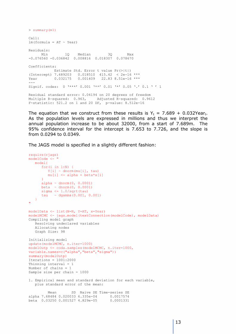
The equation that we construct from these results is Yt = 7.689 + 0.032Yeart. As the population levels are expressed in millions and thus we interpret the annual population increase to be about 32000, from a start of 7.689m. The
95% confidence interval for the intercept is 7.653 to 7.726, and the slope is from 0.0294 to 0.0349.
The JAGS model is specified in a slightly different fashion:
require(rjags)
modelCode <- "
model{
for(i in 1:N) {
Y[i] ~ dnorm(mu[i], tau)
mu[i] <- alpha + beta*x[i]
}
alpha ~ dnorm(0, 0.0001)
beta ~ dnorm(0, 0.0001)
sigma <- 1.0/sqrt(tau)
tau ~ dgamma(0.001, 0.001)
}
"
modelData <- list(N=N, Y=AT, x=Year)
modelMCMC <- jags.model(textConnection(modelCode), modelData)
Compiling model graph
Resolving undeclared variables
Allocating nodes
Graph Size: 98
Initializing model
update(modelMCMC, n.iter=1000)
modelOutp <- coda.samples(modelMCMC, n.iter=1000,
variable.names=c("alpha","beta","sigma"))
summary(modelOutp)
Iterations = 1001:2000
Thinning interval = 1
Number of chains = 1
Sample size per chain = 1000
1. Empirical mean and standard deviation for each variable,
plus standard error of the mean:
Mean SD Naive SE Time-series SE
alpha 7.68484 0.020033 6.335e-04 0.0017574
beta 0.03250 0.001527 4.829e-05 0.0001331

14
sigma 0.04456 0.007543 2.385e-04 0.0002708
2. Quantiles for each variable:
2.5% 25% 50% 75% 97.5%
alpha 7.64190 7.67253 7.68519 7.69708 7.72379
beta 0.02959 0.03148 0.03250 0.03345 0.03563
sigma 0.03289 0.03959 0.04364 0.04841 0.06311
We are required supply the observation equation for Y, the system equation for mu, and our suggestions for the prior distributions. Y will be sampled from a
normal distribution, with mean mui. The priors for the coefficients, alpha and beta, will be sampled from a normal distribution, and the precision, tau, from a
gamma distribution. In JAGS the precision tau is used to specify the variation of the samples, and if we want the value of the standard deviation, sigma, then we
must supply the deterministic identity between it and tau. We subject the model to a burn-in period of 1000 samples, and then we used
1000 samples from the Gibbs Sampler to derive the posterior distributions of the parameters. The mean values for alpha and beta are similar the OLS estimates,
and the 95% quantiles correspond to the OLS 95% confidence limits. We can also plot the distributions of the posteriors.
The density plots indicate the variability in the posterior estimates. Note that
some of the variance has been incorrectly assigned to observation variance, since the terms in the model are autocorrelated.
Tho add in an autocorrelated error term we must make further changes to the model. The autocorrelation is modelled using a multivariate normal distribution.
The mui terms are formed as before, but the autocorrelation is represented with
a covariance matrix between the terms in the series, where each entry is 2
raised to the power of the lag between the terms. The parameter r is the
measure of the autocorrelation and we sample from a beta distribution. As with the previous model, the precisions in the prior distributions are purposely small
1000 1200 1400 1600 1800 2000
7.6
07.6
57.7
07.7
5
Iterations
Trace of alpha
7.60 7.65 7.70 7.75
05
10
15
20
Density of alpha
N = 1000 Bandw idth = 0.004879
1000 1200 1400 1600 1800 2000
0.0
28
0.0
34
Iterations
Trace of beta
0.026 0.030 0.034 0.038
050
150
250
Density of beta
N = 1000 Bandw idth = 0.0003902
1000 1200 1400 1600 1800 2000
0.0
30.0
50.0
70.0
9
Iterations
Trace of sigma
0.02 0.04 0.06 0.08 0.10
010
30
50
Density of sigma
N = 1000 Bandw idth = 0.001753

15
since we have few initial views as to their values – these are known as non-informative priors.
TSmodelCode <- "
model
{
# Prior distributions
alpha ~ dnorm(0.0, 0.001)
beta ~ dnorm(0.0, 0.000001)
s2err ~ dgamma(1, 50)
rho ~ dbeta(10, 10)
# linear trend
for(i in 1:N) {
mu[i] <- alpha + beta*x[i]
}
# AR(1)
for(i in 1:N) {
for (j in 1:N) {
tdmat[i,j] <- s2err*rho^abs(i-j)
}
}
Omega <- inverse(tdmat)
Y ~ dmnorm(mu, Omega)
}
"
TSmodelData <- list(N=N, Y=AT, x=Year)
TSmodelMCMC <- jags.model(textConnection(TSmodelCode), TSmodelData)
update(TSmodelMCMC, n.iter=1000)
TSmodelOutp <- coda.samples(TSmodelMCMC, n.iter=1000,
variable.names=c("alpha","beta","rho"))
summary(TSmodelOutp)
Iterations = 2001:3000
Thinning interval = 1
Number of chains = 1
Sample size per chain = 1000
1. Empirical mean and standard deviation for each variable,
plus standard error of the mean:
Mean SD Naive SE Time-series SE
alpha 7.66386 0.034738 1.099e-03 0.0028414
beta 0.03384 0.002524 7.981e-05 0.0002024
rho 0.67646 0.088610 2.802e-03 0.0042998
2. Quantiles for each variable:
2.5% 25% 50% 75% 97.5%
alpha 7.59609 7.64060 7.66482 7.68551 7.73393
beta 0.02897 0.03227 0.03377 0.03547 0.03859
rho 0.47815 0.62342 0.68226 0.73684 0.82952
plot(TSmodelOutp)
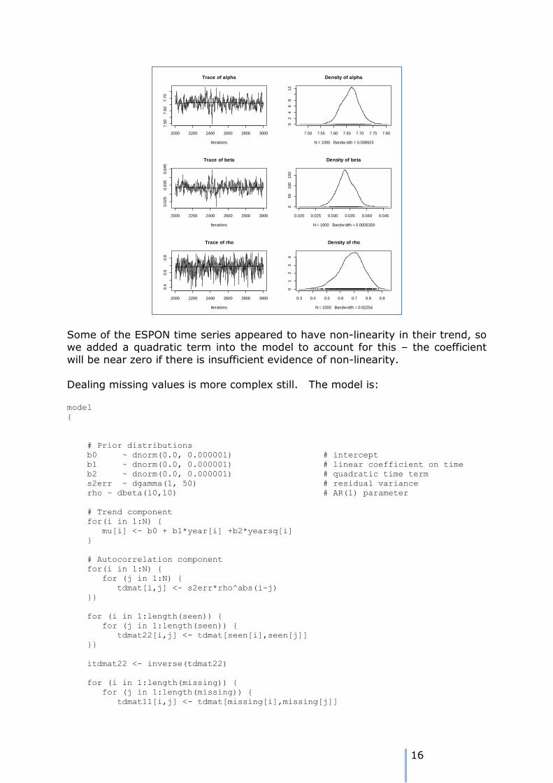
The terms in the linear trend are little different from the OLS counterparts, although the 95% quantiles are a little wider. By ignoring the autocorrelation, we underestimated the variability in the intercept and slope terms. The plot
below shows the variation in the coefficient distributions.
16
Some of the ESPON time series appeared to have non-linearity in their trend, so we added a quadratic term into the model to account for this – the coefficient
will be near zero if there is insufficient evidence of non-linearity.
Dealing missing values is more complex still. The model is: model
{
# Prior distributions
b0 ~ dnorm(0.0, 0.000001) # intercept
b1 ~ dnorm(0.0, 0.000001) # linear coefficient on time
b2 ~ dnorm(0.0, 0.000001) # quadratic time term
s2err ~ dgamma(1, 50) # residual variance
rho ~ dbeta(10,10) # AR(1) parameter
# Trend component
for(i in 1:N) {
mu[i] <- b0 + b1*year[i] +b2*yearsq[i]
}
# Autocorrelation component
for(i in 1:N) {
for (j in 1:N) {
tdmat[i,j] <- s2err*rho^abs(i-j)
}}
for (i in 1:length(seen)) {
for (j in 1:length(seen)) {
tdmat22[i,j] <- tdmat[seen[i],seen[j]]
}}
itdmat22 <- inverse(tdmat22)
for (i in 1:length(missing)) {
for (j in 1:length(missing)) {
tdmat11[i,j] <- tdmat[missing[i],missing[j]]
2000 2200 2400 2600 2800 3000
7.5
07.6
07.7
0
Iterations
Trace of alpha
7.50 7.55 7.60 7.65 7.70 7.75 7.80
02
46
812
Density of alpha
N = 1000 Bandw idth = 0.008923
2000 2200 2400 2600 2800 3000
0.0
25
0.0
35
0.0
45
Iterations
Trace of beta
0.020 0.025 0.030 0.035 0.040 0.045
050
100
150
Density of beta
N = 1000 Bandw idth = 0.0006359
2000 2200 2400 2600 2800 3000
0.4
0.6
0.8
Iterations
Trace of rho
0.3 0.4 0.5 0.6 0.7 0.8 0.9
01
23
4
Density of rho
N = 1000 Bandw idth = 0.02254

17
}}
itdmat11 <- inverse(tdmat11)
for (i in 1:length(missing)) {
for (j in 1:length(seen)) {
tdmat12[i,j] <- tdmat[missing[i],seen[j]]
}}
for (i in 1:length(seen)) {
for (j in 1:length(missing)) {
tdmat21[i,j] <- tdmat[seen[i],missing[j]]
}}
for (i in 1:length(seen)) {
mu2[i] <- mu[seen[i]]
}
for (i in 1:length(missing)) {
mu1[i] <- mu[missing[i]]
}
OmegaM <- inverse(tdmat11 - tdmat12 %*% itdmat22 %*% tdmat21)
muM <- mu1 + tdmat12 %*% itdmat22 %*% (ys - mu2)
ys ~ dmnorm(mu2,itdmat22) # non-missing data
ym ~ dmnorm(muM, OmegaM) # missing data
}
The seen and missing variables contain the indices in the time series where the
population estimates are present and missing respectively. The linkage between the missing and present values is rather more complex. These results are
standard for time series, and can be found in any time series text (e.g.: Chatfield, 1984)
The series is modelled sampling from a multivariate normal distribution, with a
vector of means resulting from the trend component, and a precision matrix (the inverse of the matrix of covariances between the terms in the series). If
there was no requirement to interpolate missing values, the precision matrix would be:
12
where 2 is the variance of the error, is the autocorrelation parameter and is
a matrix of lags. If the time series had 5 terms, would contain: [,1] [,2] [,3] [,4] [,5]
[1,] 0 1 2 3 4
[2,] 1 0 1 2 3
[3,] 2 1 0 1 2
[4,] 3 2 1 0 1
[5,] 4 3 2 1 0
The multivariate normal has density:
2
)()(
2
xTx
e

18
where is the precision and is the mean. The challenge arises when we have missing data.
The series is divided into the present and missing sub-series. The means for
each part are drawn from the trend estimate. The following covariance submatrices are required:
2221
1211
present
missing
presentmissing
The precision matrix p for the present data is:
1
22
2
This missing and present terms are linked through the precision matrix used to
estimate the posterior distributions of the missing terms, m thus:
1
21
1
221211 )( m
As well as there being more individual steps in this model, the estimation
requires two matrix inversions. In estimations for the ESPON data, the 250000 simulations were used for the burn-in process, and 100000 for the actual
sampling. Even so, on a relatively sluggish machine, about 105 seconds were used when estimation a model on data with 22 time periods and 54% of the data missing.
Spatial coherence
The second component requires a set of constraints to ensure that predictions for NUTS3 units sum to the
appropriate value for their containing NUTS2 units, and that predictions for NUTS2 units sum to the
appropriate value for the containing NUTS1 units as so on. We refer to this as hierarchical spatial coherence. If we have a NUTS2 region with population P, and we
know the populations of three of its, say 5, units, a, b and c, but not d and e, then we can include
P=a+b+c+d+e as a constraint in the Bayesian forecasting framework. This is accomplished via a prior probability distribution: a+b+c+d+e will take the
P with a probability of 1, and zero otherwise. In this fashion we can ensure spatial coherence in the
forecasts. In practice the application of the this constraint occurs after the individual series
have been estimated - we apply an adjustment to the individual NUTS3 region

19
estimates to the estimates so that their total is that of the containing NUTS2 region. This adjustment applies from the NUTS1 regions downwards to ensure
the spatial coherence of the estimates. It has to be remembered that we are not appling a pro-rata to a series of individual estimates, we are adding the posterior
distributions together. The highest posterior density of the summed series is the value of the constraining total.
The same idea applies for those data that are considered to be embarrassingly estimatable. Suppose the know the populations of a NUTS2 region, and 3 of the
4 NUTS3 regions which are contained within it. Then PNUTS3,4 = PNUTS2 - (PNUTS3,1+PNUTS3,2+PNUTS3,3). The known data can be considered to be sampled from a distribution with a mean corresponding to the known value and infinite
precision (i.e. the variance is zero). The known value is then the highest posterior density value, and it has a probability of 1 (with a variance of zero,
there can be no other probability!). Similarly the situation where a NUTS2 value is missing, but the underling NUTS3
values are present, then the same approach yields the estimate PNUTS2 = PNUTS3,1+PNUTS3,2+PNUTS3,3+ PNUTS3,4. Again, the known NUTS3 values are
assumed to be sampled from a distribution with a mean of PNUTS3,x and an infinite precision - which means that the known values have a posterior probability of 1.
The resulting posterior distribution for the PNUTS2 total also has a probability of 1. We require one further component in operationalisation of the method: a means
of identifying the various scenarios and considering the hierarchical coherence. The files of data from Eurostat and the National Statistical agencies usually have
the NUTS codes in a single column, and a flat file structure: the rows represent spatial units and the columns variables of interest. This effective;y flattens the hierarchical stricture of the NUTS units, and, if the calculations are restricted to
the spreadsheet, renders the task of ensuring hierarchical coherence enormously difficult. An alternative to use the conceptual representation of the BUTS units as
belong to some sort of tree structure – like a family tree – in which the higher level units are represented as the parents of lower level units.
Tree structures are extensively used in computer science to represent data. A tree many defined as having a root and one or more subtrees each of which is a
tree. For each country, the root is the NUTS0 region, and the NUTS1 regions are the first subtrees. Each NUTS1 subtree has corresponding NUTS2 subtrees, and each NUTS2 region has corresponding NUTS3 subtrees.
The example shows the NUTS hierarchy for the Netherlands. We can see the
hierarchy clearly and explicitly. It also forms the basis for the software implementation of the MCMC approach.
Other issues
One issue which will have to be faced is that of ensuring temporal coherence for the changes that have taken place in the system of NUTS units over the years. Boundaries of zones may be shifted, zones may be merged, and zones may be
split. Correspondance tables are available at EUROSTAT.
20
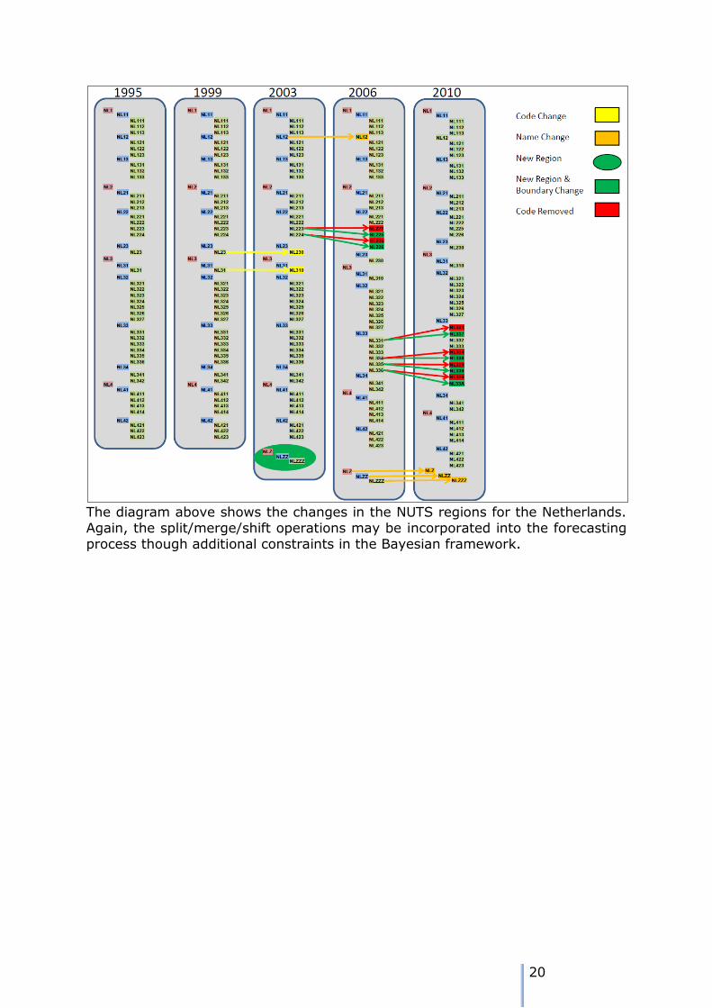
The diagram above shows the changes in the NUTS regions for the Netherlands. Again, the split/merge/shift operations may be incorporated into the forecasting process though additional constraints in the Bayesian framework.
21
p1
99
0
p1
99
1
p1
99
2
p1
99
3
p1
99
4
p1
99
5
p1
99
6
p1
99
7
p1
99
8
p1
99
9
p2
00
0
p2
00
1
p2
00
2
p2
00
3
p2
00
4
p2
00
5
p2
00
6
p2
00
7
p2
00
8
p2
00
9
p2
01
0
p2
01
1
Year
AT342AT341AT335AT334AT333AT332AT331AT323AT322AT321AT315AT314AT313AT312AT311AT226AT225AT224AT223AT222AT221AT213AT212AT211AT130AT127AT126AT125AT124AT123AT122AT121AT113AT112AT111AT34AT33AT32AT31AT22AT21AT13AT12AT11AT3AT2AT1AT
NU
TS
Re
gio
n
Austria Unadjusted Populations
4. Implementation
How are we to implement this? We will require bespoke code, and we will require a means of both handling the Excel spreadsheets, the NUTS hierarchy, and the computations required for the estimating of the missing data.
Software for MCMC approaches has been, until recently, the province of the
specialist. This altered with the release of BUGS (Bayesian inference Using Gibbs Sampling) (Lunn et al., 2009, 2012). BUGS has now been extended with a
Windows interface (WinBUGS) and to handle spatial data (GeoBUGS). However, data preparation, and post-modelling evaluation requires other software. The release of JAGS (Just Another Gibbs Sampler) (Plummer, 2003) provides a
further milestone. This offers a very similar facility to BUGS, but it is open source and may also be used in conjunction with the statistical programming
language R via the rjags package in R. This offers R users the capability of fitting models using MCMC, but also exploits the power and flexibility of R, in order to prepare the data, and to provide extensive evaluation of the results. Using JAGS
it is possible to obtain posterior distribution for the parameters outlined in the previous sections, and for the missing data. It is also worth noting that this
approach also allows the constraint that the sum of all of the NUTS3 regions within a NUTS2 region must equal the statistic associate with that NUTS2 region.
The R package has also been used to implement the data checking procedures, and the RIATE team have also made use of R.
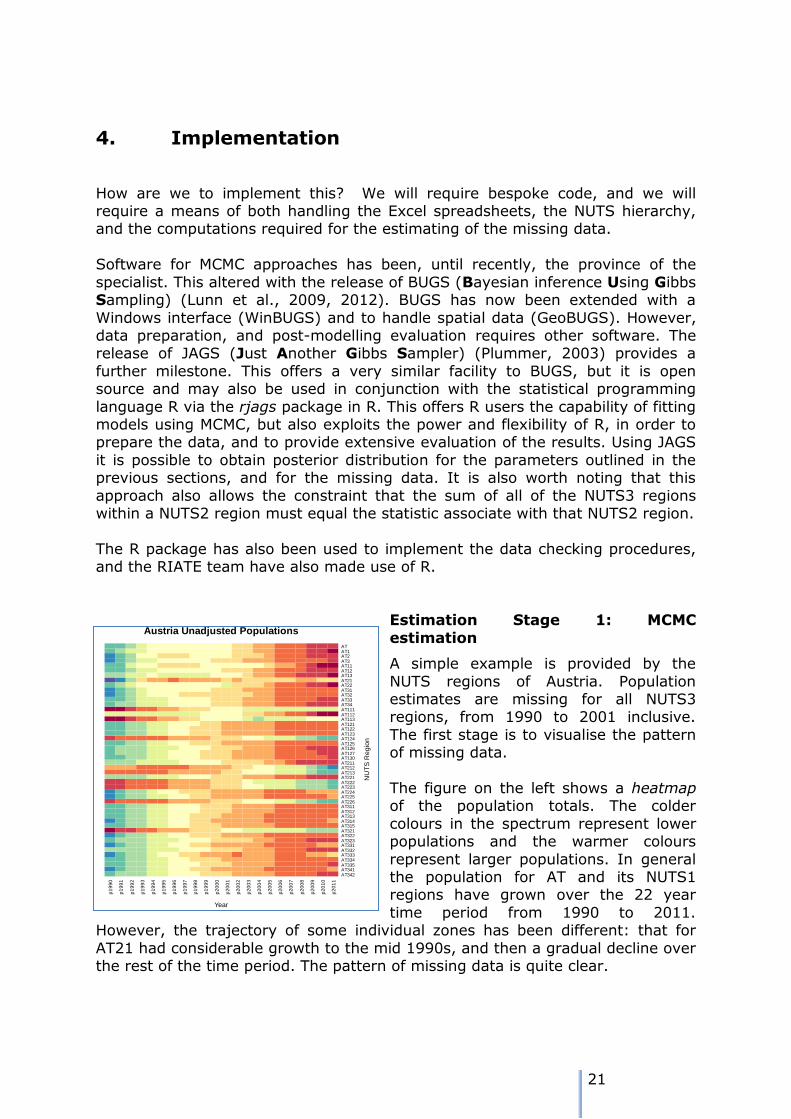
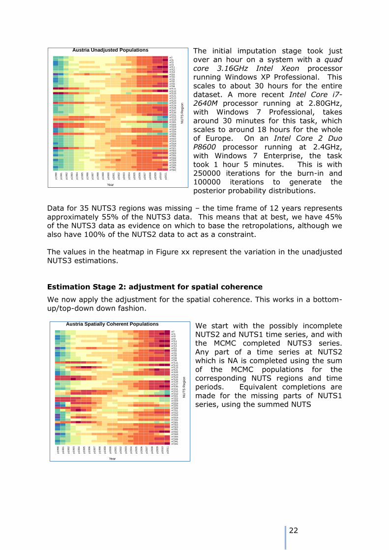
Estimation Stage 1: MCMC
estimation
A simple example is provided by the
NUTS regions of Austria. Population estimates are missing for all NUTS3 regions, from 1990 to 2001 inclusive.
The first stage is to visualise the pattern of missing data.
The figure on the left shows a heatmap of the population totals. The colder
colours in the spectrum represent lower populations and the warmer colours
represent larger populations. In general the population for AT and its NUTS1 regions have grown over the 22 year
time period from 1990 to 2011. However, the trajectory of some individual zones has been different: that for
AT21 had considerable growth to the mid 1990s, and then a gradual decline over the rest of the time period. The pattern of missing data is quite clear.
22
p1
99
0
p1
99
1
p1
99
2
p1
99
3
p1
99
4
p1
99
5
p1
99
6
p1
99
7
p1
99
8
p1
99
9
p2
00
0
p2
00
1
p2
00
2
p2
00
3
p2
00
4
p2
00
5
p2
00
6
p2
00
7
p2
00
8
p2
00
9
p2
01
0
p2
01
1
Year
AT342AT341AT335AT334AT333AT332AT331AT323AT322AT321AT315AT314AT313AT312AT311AT226AT225AT224AT223AT222AT221AT213AT212AT211AT130AT127AT126AT125AT124AT123AT122AT121AT113AT112AT111AT34AT33AT32AT31AT22AT21AT13AT12AT11AT3AT2AT1AT
NU
TS
Re
gio
n
Austria Unadjusted Populations
p1
99
0
p1
99
1
p1
99
2
p1
99
3
p1
99
4
p1
99
5
p1
99
6
p1
99
7
p1
99
8
p1
99
9
p2
00
0
p2
00
1
p2
00
2
p2
00
3
p2
00
4
p2
00
5
p2
00
6
p2
00
7
p2
00
8
p2
00
9
p2
01
0
p2
01
1
Year
AT342AT341AT335AT334AT333AT332AT331AT323AT322AT321AT315AT314AT313AT312AT311AT226AT225AT224AT223AT222AT221AT213AT212AT211AT130AT127AT126AT125AT124AT123AT122AT121AT113AT112AT111AT34AT33AT32AT31AT22AT21AT13AT12AT11AT3AT2AT1AT
NU
TS
Re
gio
n
Austria Spatially Coherent Populations
The initial imputation stage took just over an hour on a system with a quad
core 3.16GHz Intel Xeon processor running Windows XP Professional. This
scales to about 30 hours for the entire dataset. A more recent Intel Core i7-2640M processor running at 2.80GHz,
with Windows 7 Professional, takes around 30 minutes for this task, which
scales to around 18 hours for the whole of Europe. On an Intel Core 2 Duo P8600 processor running at 2.4GHz,
with Windows 7 Enterprise, the task took 1 hour 5 minutes. This is with
250000 iterations for the burn-in and 100000 iterations to generate the posterior probability distributions.
Data for 35 NUTS3 regions was missing – the time frame of 12 years represents
approximately 55% of the NUTS3 data. This means that at best, we have 45% of the NUTS3 data as evidence on which to base the retropolations, although we
also have 100% of the NUTS2 data to act as a constraint. The values in the heatmap in Figure xx represent the variation in the unadjusted
NUTS3 estimations.
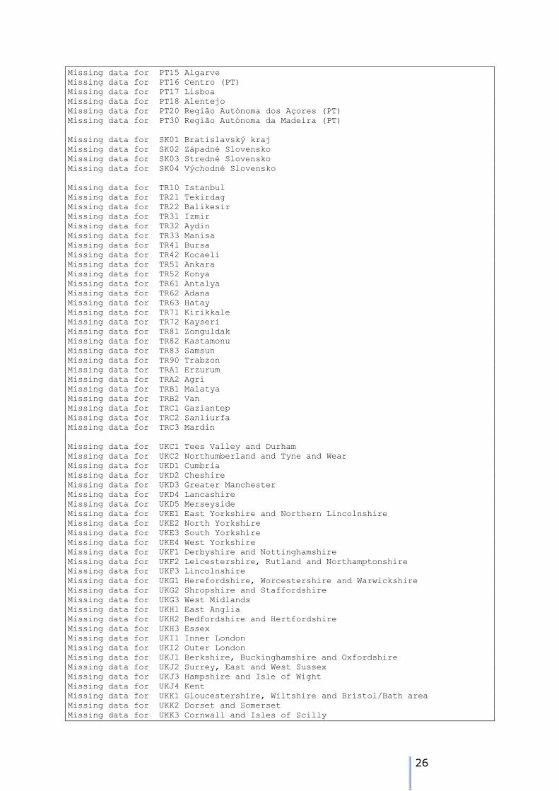
Estimation Stage 2: adjustment for spatial coherence
We now apply the adjustment for the spatial coherence. This works in a bottom-
up/top-down down fashion.
We start with the possibly incomplete NUTS2 and NUTS1 time series, and with the MCMC completed NUTS3 series.
Any part of a time series at NUTS2 which is NA is completed using the sum
of the MCMC populations for the corresponding NUTS regions and time periods. Equivalent completions are
made for the missing parts of NUTS1 series, using the summed NUTS

23
From this it can be seen that missing data in the NUTS0, NUTS1 and NUTS2 regions can be a challenge. We can determine appropriate strategies by
examining some cases from the data.
Consider the case of Croatia. A portion of the times series for all of the NUTS regions in Croatia is shown below: > Data.estim[Country == "HR",4:16]
p1990 p1991 p1992 p1993 p1994 p1995 p1996 p1997 p1998 p1999 p2000 p2001 p2002
HR 4778007 4784265 4470266 4641275 4649034 4668752 4493581 4572474 4501149 4553769 4381352 4437460 4444608
HR0 4778007 4784265 4470266 4641275 4649034 4668752 4493581 4572474 4501149 4553769 4381352 4437460 4444608
HR01 NA 1646710 NA NA NA NA NA NA NA NA NA NA 1661396
HR02 NA 1557342 NA NA NA NA NA NA NA NA NA NA 1349105
HR03 NA 1580213 NA NA NA NA NA NA NA NA NA NA 1434107
HR011 NA 777826 NA NA NA NA NA NA NA NA NA 779145 780332
HR012 NA 282989 NA NA NA NA NA NA NA NA NA 309696 312046
HR013 NA 148779 NA NA NA NA NA NA NA NA NA 142432 141886
HR014 NA 187853 NA NA NA NA NA NA NA NA NA 184769 184420
HR015 NA 129397 NA NA NA NA NA NA NA NA NA 124467 124161
HR016 NA 119866 NA NA NA NA NA NA NA NA NA 118426 118551
HR021 NA 144042 NA NA NA NA NA NA NA NA NA 133084 132499
HR022 NA 104625 NA NA NA NA NA NA NA NA NA 93389 93029
HR023 NA 99334 NA NA NA NA NA NA NA NA NA 85831 85819
HR024 NA 174998 NA NA NA NA NA NA NA NA NA 176765 177143
HR025 NA 367193 NA NA NA NA NA NA NA NA NA 330506 330293
HR026 NA 231241 NA NA NA NA NA NA NA NA NA 204768 204455
HR027 NA 184577 NA NA NA NA NA NA NA NA NA 141787 141069
HR028 NA 251332 NA NA NA NA NA NA NA NA NA 185387 184798
HR031 NA 323130 NA NA NA NA NA NA NA NA NA 305505 305652
HR032 NA 85135 NA NA NA NA NA NA NA NA NA 53677 53466
HR033 NA 214777 NA NA NA NA NA NA NA NA NA 162045 163642
HR034 NA 152477 NA NA NA NA NA NA NA NA NA 112891 113406
HR035 NA 474019 NA NA NA NA NA NA NA NA NA 463676 467300
HR036 NA 204346 NA NA NA NA NA NA NA NA NA 206344 207112
HR037 NA 126329 NA NA NA NA NA NA NA NA NA 122870 123529
In 2001 all the NUTS3 data are present at NUTS1 and NUTS3, but not for
NUTS2. As none of the NUTS3 values are estimates, then they can be summed over the NUTS2 codes to obtain the desired totals: > tapply(HR[6:26,"p2001"],substr(rownames(HR)[6:26],1,4),sum)
HR01 HR02 HR03
1658935 1351517 1427008
The missing data for NUTS2 and NUTS3 from 1992 to 2000 require two levels of constraint:
1. Use MCMC to estimate values for 1992 to 2000 for all the missing data points 2. Constrain the NUTS2 MCMC estimates to the NUTS1 value 3. Constrain the NUTS3 MCMC estimates to the newly constrained NUTS2 values
This is easily programmed accommodated in the constraining function, as we
traverse the tree from the root downwards. By the time we deal with the NUTS3 estimates, the NUTS2 will have been constrained.
In the case of Portugal, there are some other special cases: > Data.estim[substr(rownames(Data.estim),1,2)=="PT",]
UnitCode Level Name p1990 p1991 p1992 p1993 p1994 p1995 p1996
PT PT NUTS0 Portugal 9970441 9912140 NA NA NA NA 10043180
PT1 PT1 NUTS1 Continente NA NA NA NA NA NA 9556916
PT2 PT2 NUTS1 Região Autónoma dos Açores (PT) NA NA 239336 239271 239207 238807 238272
PT3 PT3 NUTS1 Região Autónoma da Madeira (PT) NA NA 253999 253059 252120 250165 247992
PT11 PT11 NUTS2 Norte NA NA 3511771 3516484 3527789 3541805 3555975
PT15 PT15 NUTS2 Algarve NA NA 341075 343336 345970 349658 353309
PT16 PT16 NUTS2 Centro (PT) NA NA 2272111 2270518 2271336 2276261 2281286
PT17 PT17 NUTS2 Lisboa NA NA 2574265 2581419 2585705 2593283 2599990
PT18 PT18 NUTS2 Alentejo NA NA 772760 770509 768468 767593 766356
PT20 PT20 NUTS2 Região Autónoma dos Açores (PT) NA NA 239336 239271 239207 238807 238272
PT30 PT30 NUTS2 Região Autónoma da Madeira (PT) NA NA 253999 253059 252120 250165 247992
PT111 PT111 NUTS3 Minho-Lima NA NA 252188 251518 250382 249541 248771
PT112 PT112 NUTS3 Cávado NA NA 358355 360519 363498 366785 369787

24
The NUTS0 and NUTS1 values are missing for 1992 to 1995 for PT1. However, there is complete coverage of PT1 at NUTS2, so the value for PT1 can be
obtained by direct summation over the corresponding NUTS2 values. The NUTS0 values can then be completed for those years as well.
It would be beneficial to be able to do this prior to MCMC since it is a deterministic operation and provide extra evidence for the MCMC estimation of
the PT1 series for 1990 and 1991. Apart from the NUTS0 total, all other data for 1990 and 1991 is missing.
The strategy for 1990 and 1991 follows the top-down strategy outlined above, and provides a general case:
1. Constrain the NUTS1 MCMC estimates to the NUTS0 total 2. Constrain the NUTS2 MCMC estimates to the constrained NUTS1 values 3. Constrain the NUTS3 MCMC estimates to the constrained NUTS2 values
Again, this can be easily accomplished using the tree traversal algorithm.
Turkey is rather more of a challenge.
UnitCode Level Name p1990 p1991 p1992 p1993 p1994 p1995 p1996 p1997
TR TR NUTS0 Turkey 56473035 NA NA NA NA NA NA NA
p1998 p1999 p2000 p2001 p2002 p2003 p2004 p2005 p2006 p2007 p2008
TR NA NA 67803927 NA NA NA NA NA NA NA 70586256
p2009 p2010 p2011
TR 71517100 72561312 73722988
Data are present only for 1990, 2000, 2008-2011 for all NUTS regions, including NUTS0. The strategy here will be to estimate all the missing data using the
MCMC technique. Then, we apply the hierarchical constraint working down the tree from NUTS0 to NUTS1, NUTS1 to NUTS2 and finally NUTS2 to NUTS3.
NUTS0, NUTS1 and NUTS2 regions with missing data are listed below: Missing data for PT Portugal
Missing data for TR Turkey
Missing data for UK United Kingdom
**************** NUTS1 Missing ******************************************
Missing data for FR9 Départements d'outre-mer (FR)
Missing data for NL3 West-Nederland
Missing data for PL1 Region Centralny
Missing data for PL2 Region Poludniowy
Missing data for PL3 Region Wschodni
Missing data for PL4 Region Pólnocno-Zachodni
Missing data for PL5 Region Poludniowo-Zachodni
Missing data for PL6 Region Pólnocny
Missing data for PT1 Continente
Missing data for PT2 Região Autónoma dos Açores (PT)
Missing data for PT3 Região Autónoma da Madeira (PT)
Missing data for TR1 Istanbul
Missing data for TR2 Bati Marmara
Missing data for TR3 Ege
Missing data for TR4 Dogu Marmara

25
Missing data for TR5 Bati Anadolu
Missing data for TR6 Akdeniz
Missing data for TR7 Orta Anadolu
Missing data for TR8 Bati Karadeniz
Missing data for TR9 Dogu Karadeniz
Missing data for TRA Kuzeydogu Anadolu
Missing data for TRB Ortadogu Anadolu
Missing data for TRC Güneydogu Anadolu
Missing data for UKC North East (UK)
Missing data for UKD North West (UK)
Missing data for UKE Yorkshire and The Humber
Missing data for UKF East Midlands (UK)
Missing data for UKG West Midlands (UK)
Missing data for UKH East of England
Missing data for UKI London
Missing data for UKJ South East (UK)
Missing data for UKK South West (UK)
Missing data for UKL Wales
Missing data for UKM Scotland
Missing data for UKN Northern Ireland (UK)
**************** NUTS2 Missing ******************************************
Missing data for CZ01 Praha
Missing data for CZ02 Strední Cechy
Missing data for CZ03 Jihozápad
Missing data for CZ04 Severozápad
Missing data for CZ05 Severovýchod
Missing data for CZ06 Jihovýchod
Missing data for CZ07 Strední Morava
Missing data for CZ08 Moravskoslezsko
Missing data for DE41 Brandenburg - Nordost
Missing data for DE42 Brandenburg - Südwest
Missing data for DED1 Chemnitz
Missing data for DED2 Dresden
Missing data for DED3 Leipzig
Missing data for DK01 Hovedstaden
Missing data for DK02 Sjælland
Missing data for DK03 Syddanmark
Missing data for DK04 Midtjylland
Missing data for DK05 Nordjylland
Missing data for HR01 Sjeverozapadna Hrvatska
Missing data for HR02 Sredisnja i Istocna (Panonska) Hrvatska
Missing data for HR03 Jadranska Hrvatska
Missing data for IE01 Border, Midland and Western
Missing data for IE02 Southern and Eastern
Missing data for PL11 Lódzkie
Missing data for PL12 Mazowieckie
Missing data for PL21 Malopolskie
Missing data for PL22 Slaskie
Missing data for PL31 Lubelskie
Missing data for PL32 Podkarpackie
Missing data for PL33 Swietokrzyskie
Missing data for PL34 Podlaskie
Missing data for PL41 Wielkopolskie
Missing data for PL42 Zachodniopomorskie
Missing data for PL43 Lubuskie
Missing data for PL51 Dolnoslaskie
Missing data for PL52 Opolskie
Missing data for PL61 Kujawsko-Pomorskie
Missing data for PL62 Warminsko-Mazurskie
Missing data for PL63 Pomorskie
Missing data for PT11 Norte
26
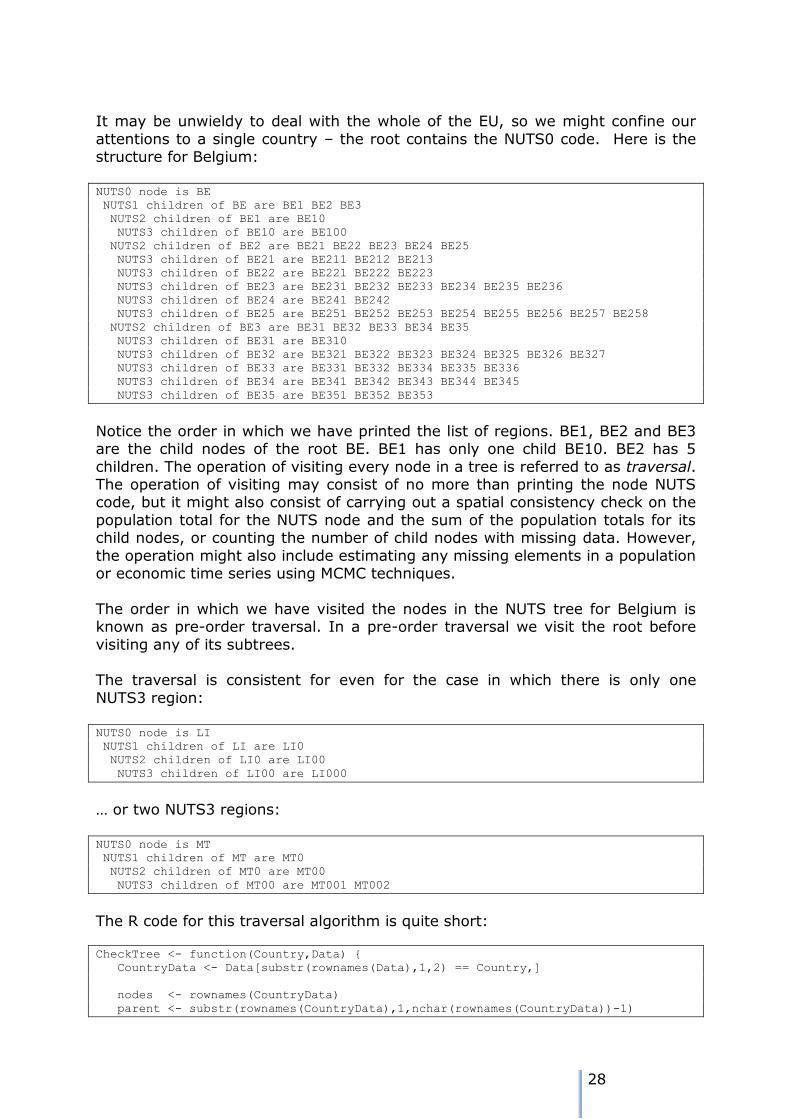
Missing data for PT15 Algarve
Missing data for PT16 Centro (PT)
Missing data for PT17 Lisboa
Missing data for PT18 Alentejo
Missing data for PT20 Região Autónoma dos Açores (PT)
Missing data for PT30 Região Autónoma da Madeira (PT)
Missing data for SK01 Bratislavský kraj
Missing data for SK02 Západné Slovensko
Missing data for SK03 Stredné Slovensko
Missing data for SK04 Východné Slovensko
Missing data for TR10 Istanbul
Missing data for TR21 Tekirdag
Missing data for TR22 Balikesir
Missing data for TR31 Izmir
Missing data for TR32 Aydin
Missing data for TR33 Manisa
Missing data for TR41 Bursa
Missing data for TR42 Kocaeli
Missing data for TR51 Ankara
Missing data for TR52 Konya
Missing data for TR61 Antalya
Missing data for TR62 Adana
Missing data for TR63 Hatay
Missing data for TR71 Kirikkale
Missing data for TR72 Kayseri
Missing data for TR81 Zonguldak
Missing data for TR82 Kastamonu
Missing data for TR83 Samsun
Missing data for TR90 Trabzon
Missing data for TRA1 Erzurum
Missing data for TRA2 Agri
Missing data for TRB1 Malatya
Missing data for TRB2 Van
Missing data for TRC1 Gaziantep
Missing data for TRC2 Sanliurfa
Missing data for TRC3 Mardin
Missing data for UKC1 Tees Valley and Durham
Missing data for UKC2 Northumberland and Tyne and Wear
Missing data for UKD1 Cumbria
Missing data for UKD2 Cheshire
Missing data for UKD3 Greater Manchester
Missing data for UKD4 Lancashire
Missing data for UKD5 Merseyside
Missing data for UKE1 East Yorkshire and Northern Lincolnshire
Missing data for UKE2 North Yorkshire
Missing data for UKE3 South Yorkshire
Missing data for UKE4 West Yorkshire
Missing data for UKF1 Derbyshire and Nottinghamshire
Missing data for UKF2 Leicestershire, Rutland and Northamptonshire
Missing data for UKF3 Lincolnshire
Missing data for UKG1 Herefordshire, Worcestershire and Warwickshire
Missing data for UKG2 Shropshire and Staffordshire
Missing data for UKG3 West Midlands
Missing data for UKH1 East Anglia
Missing data for UKH2 Bedfordshire and Hertfordshire
Missing data for UKH3 Essex
Missing data for UKI1 Inner London
Missing data for UKI2 Outer London
Missing data for UKJ1 Berkshire, Buckinghamshire and Oxfordshire
Missing data for UKJ2 Surrey, East and West Sussex
Missing data for UKJ3 Hampshire and Isle of Wight
Missing data for UKJ4 Kent
Missing data for UKK1 Gloucestershire, Wiltshire and Bristol/Bath area
Missing data for UKK2 Dorset and Somerset
Missing data for UKK3 Cornwall and Isles of Scilly

27
Missing data for UKK4 Devon
Missing data for UKL1 West Wales and The Valleys
Missing data for UKL2 East Wales
Missing data for UKM2 Eastern Scotland
Missing data for UKM3 South Western Scotland
Missing data for UKM5 North Eastern Scotland
Missing data for UKM6 Highlands and Islands
Missing data for UKN0 Northern Ireland (UK)
The NUTS regions structures and missing data
The spreadsheet provides a poor model for the NUTS hierarchy. The rows can
be sorted on the NUTS codes sot that the first part of the spreadsheet represents country information, the NUTS1 regions are next, followed by NUTS2
and NUTS3. However, we can't easily identify quickly a NUTS2 region, and then its constituent NUTS3 regions – it may be possible to do this with lookup in an auxiliary table, but this does not provide any flexibility. From the point of
estimating missing data, the requirement for spatial coherence requires us to be able to identify these relationships in the data quickly and consistently. We refer
to the NUTS hierarchy, but have no mechanism for representing and using that hierarchy.
The solution is to create a data structure and associated travel algorithms so that we can work on the regions in a consistent fashion. An appropriate data
structure is the tree. Trees are used widely in computer science for organising and searching for information. In the computing section of many academic bookshops there will be volumes with titles like Data Structures and Algorithms.
A classic collection is the volumes in the series The Art of Computer Programming by Professor Donald Knuth. Knuth defines a tree thus:
"… a finite set T of one or more nodes such that
a) There is one specially designated node called the root of the tree, root(T); and b) The remaining nodes (excluding the root) are partitioned into m >= 0 disjoint sets T1,
… Tm and each of these sets in turn is a tree. The trees T1, … Tm are called the subtrees of the root."10
This definition is recursive – the tree is defined in terms of trees. Put another
way: a tree consists of a root and one or more nodes, each of which is a tree. A root which has no nodes is called a leaf node. There is an analogy with a family
tree – a structure much used in genealogy: the non-root nodes are the children and the root represents the parents. As each node is itself a tree, we can also refer to the nodes as subtrees, because each is a tree.
The NUTS hierarchy can be represented as a tree quite naturally in terms of this
definition. A node could consist of the NUTS code, and NUTS level and perhaps the population. The root would be the EU, and its 34 nodes contain the 34 NUTS0 codes, the value 0 for the level, and the national population. Each of
these 34 nodes is itself a tree. Each NUTS0 nodes has one or more NUTS1 nodes, and in turn each NUTS1 node has one or more NUTS2 nodes and so on.
10 Knuth DE, 1973, Fundamental Algorithms, The Art of Computer Programming, Volume
1, Reading MA: Addison-Wesley, p305
28
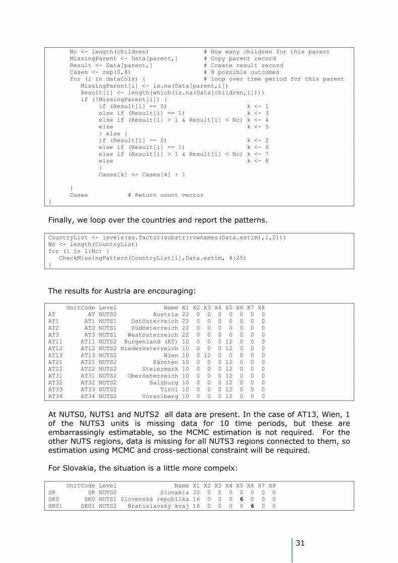
It may be unwieldy to deal with the whole of the EU, so we might confine our
attentions to a single country – the root contains the NUTS0 code. Here is the structure for Belgium:
NUTS0 node is BE
NUTS1 children of BE are BE1 BE2 BE3
NUTS2 children of BE1 are BE10
NUTS3 children of BE10 are BE100
NUTS2 children of BE2 are BE21 BE22 BE23 BE24 BE25
NUTS3 children of BE21 are BE211 BE212 BE213
NUTS3 children of BE22 are BE221 BE222 BE223
NUTS3 children of BE23 are BE231 BE232 BE233 BE234 BE235 BE236
NUTS3 children of BE24 are BE241 BE242
NUTS3 children of BE25 are BE251 BE252 BE253 BE254 BE255 BE256 BE257 BE258
NUTS2 children of BE3 are BE31 BE32 BE33 BE34 BE35
NUTS3 children of BE31 are BE310
NUTS3 children of BE32 are BE321 BE322 BE323 BE324 BE325 BE326 BE327
NUTS3 children of BE33 are BE331 BE332 BE334 BE335 BE336
NUTS3 children of BE34 are BE341 BE342 BE343 BE344 BE345
NUTS3 children of BE35 are BE351 BE352 BE353
Notice the order in which we have printed the list of regions. BE1, BE2 and BE3 are the child nodes of the root BE. BE1 has only one child BE10. BE2 has 5
children. The operation of visiting every node in a tree is referred to as traversal. The operation of visiting may consist of no more than printing the node NUTS code, but it might also consist of carrying out a spatial consistency check on the
population total for the NUTS node and the sum of the population totals for its child nodes, or counting the number of child nodes with missing data. However,
the operation might also include estimating any missing elements in a population or economic time series using MCMC techniques.
The order in which we have visited the nodes in the NUTS tree for Belgium is known as pre-order traversal. In a pre-order traversal we visit the root before
visiting any of its subtrees. The traversal is consistent for even for the case in which there is only one
NUTS3 region: NUTS0 node is LI
NUTS1 children of LI are LI0
NUTS2 children of LI0 are LI00
NUTS3 children of LI00 are LI000
… or two NUTS3 regions: NUTS0 node is MT
NUTS1 children of MT are MT0
NUTS2 children of MT0 are MT00
NUTS3 children of MT00 are MT001 MT002
The R code for this traversal algorithm is quite short:
CheckTree <- function(Country,Data) {
CountryData <- Data[substr(rownames(Data),1,2) == Country,]
nodes <- rownames(CountryData)
parent <- substr(rownames(CountryData),1,nchar(rownames(CountryData))-1)

29
parent[1] <- ""
ROOT <- which(nodes == Country)
cat("\nTree Walk\n")
root <- nodes[ROOT]
cat("NUTS0 node is ",root,"\n")
children1 <- nodes[parent == root]
cat(" NUTS1 children of", root, "are", children1,"\n")
Nc1 <- length(children1)
for (i in 1:Nc1) {
node2 <- children1[i]
children2 <- nodes[parent == node2]
cat(" NUTS2 children of", node2, "are", children2,"\n")
Nc2 <- length(children2)
for (j in 1:Nc2) {
node3 <- children2[j]
children3 <- nodes[parent == node3]
cat(" NUTS3 children of", node3, "are", children3,"\n")
}
}
}
The argument County contains the two character country code for the country of
interest. The argument Data is the data matrix for Europe, where the rows have
been indexed by their NUTS code. In our example, the first column of Data contains the NUTS code, code the indexing takes the form of:
Rownames(Data) <- Data[,1]
The tree for any desired country can be printed by calling the function with the appropriate country code. For the examples above we used: CheckTree("BE",Data)
CheckTree("LI",Data)
CheckTree("MT",Data)
Missing data patterns in the ESPON time series
There are 8 possible patterns of missing data for each node. We can use the tree walk algorithm presented earlier to traverse the tree, and examine the
patterns. As we visit each node, then we can tabulate the different patterns over the 22 years of the time series in the example.
The cases that arise for any selected time period are: Case Parent node Child nodes Note
1 Data present All data present No estimation required
2 Data missing All data present Parent can be computed
3 Data present 1 child node missing data Child node embarrassingly estimatable
4 Data present Some child nodes missing data Estimation/constraint required
5 Data present All child nodes missing data Estimation/constraint required
6 Data missing 1 child node missing data Higher order estimation required
7 Data missing Some child nodes missing data Higher order estimation required
8 Data missing All child nodes missing data Higher order estimation required
As we move down the table, the problem for the estimation strategy becomes more complex. Case 1 requires no action – all the data are present. Case 2 and

30
case 3 are examples of emabrassingly estimatable situations, the child or parent node data can be computed directly from the available data. Cases 4 and 5
require estimation of the child series using MCMC, and then application of the cross-sectional constraint. Cases 6, 7 and 8 are more challenging, and require
estimation of the higher order data in order to provide the cross-sectional constraints.
The patterns can either be visualised using a heatmap – these are shown in Appendix 7. We can also use the tree traversal algorithm and a pattern analyser
to check the patterns at each node. A sutiable tree traversal function is shown below. As each node is visited, the pattern of cases over the time periods is computed, and the stored in a data frame.
CheckMissingPattern <- function(Country,Data,dataCols,verbose=FALSE) {
CountryData <- Data[substr(rownames(Data),1,2) == Country,]
IDInfo <- CountryData[,1:3]
Nc <- dim(IDInfo)[1]
Results <- data.frame(IDInfo[,1:3],matrix(0,Nc,8))
rownames(Results) <- rownames(CountryData)
nodes <- rownames(CountryData)
parent <- substr(rownames(CountryData),1,nchar(rownames(CountryData))-1)
parent[1] <- ""
Nd <- length(dataCols)
### visit.node
### for each child(visit.node)
ROOT <- which(nodes == Country)
if Iverbose) cat("\nTree Walk\n")
root <- nodes[ROOT]
if (verbose) cat("NUTS0 node is ",root,"\n")
children1 <- nodes[parent == root]
if (verbose) cat(" NUTS1 children of", root, "are", children1,"\n")
Nc1 <- length(children1)
CasePattern <- CheckNode(root,children1,Data,dataCols)
Results[root,4:11] <- CasePattern
for (i in 1:Nc1) {
node2 <- children1[i]
children2 <- nodes[parent == node2]
if (verbose) cat(" NUTS2 children of", node2, "are", children2,"\n")
Nc2 <- length(children2)
CasePattern <- CheckNode(node2,children2,Data,dataCols)
Results[node2,4:11] <- CasePattern
for (j in 1:Nc2) {
node3 <- children2[j]
children3 <- nodes[parent == node3]
if (verbose) cat(" NUTS3 children of",node3,"are", children3,"\n")
Nc3 <- length(children3)
CasePattern <- CheckNode(node3,children3,Data,dataCols)
Results[node3,4:11] <- CasePattern
}
}
NUTSlevels <- lapply(Results[,2], as.character)
print(Results[NUTSlevels <= "NUTS2",])
}
This requires a function to carry out the analysis of the missing data patterns associated with each node:
CheckNode <- function(parent,children,Data,dataCols){
31
Nc <- length(children) # How many children for this parent
MissingParent <- Data[parent,] # Copy parent record
Result <- Data[parent,] # Create result record
Cases <- rep(0,8) # 8 possible outcomes
for (i in dataCols) { # loop over time period for this parent
MissingParent[i] <- is.na(Data[parent,i])
Result[i] <- length(which(is.na(Data[children,i])))
if (!MissingParent[i]) {
if (Result[i] == 0) k <- 1
else if (Result[i] == 1) k <- 3
else if (Result[i] > 1 & Result[i] < Nc) k <- 4
else k <- 5
} else {
if (Result[i] == 0) k <- 2
else if (Result[i] == 1) k <- 6
else if (Result[i] > 1 & Result[i] < Nc) k <- 7
else k <- 8
}
Cases[k] <- Cases[k] + 1
}
Cases # Return count vector
}
Finally, we loop over the countries and report the patterns. CountryList <- levels(as.factor(substr(rownames(Data.estim),1,2)))
Nc <- length(CountryList)
for (i in 1:Nc) {
CheckMissingPattern(CountryList[i],Data.estim, 4:25)
}
The results for Austria are encouraging:
UnitCode Level Name X1 X2 X3 X4 X5 X6 X7 X8
AT AT NUTS0 Austria 22 0 0 0 0 0 0 0
AT1 AT1 NUTS1 Ostösterreich 22 0 0 0 0 0 0 0
AT2 AT2 NUTS1 Südösterreich 22 0 0 0 0 0 0 0
AT3 AT3 NUTS1 Westösterreich 22 0 0 0 0 0 0 0
AT11 AT11 NUTS2 Burgenland (AT) 10 0 0 0 12 0 0 0
AT12 AT12 NUTS2 Niederösterreich 10 0 0 0 12 0 0 0
AT13 AT13 NUTS2 Wien 10 0 12 0 0 0 0 0
AT21 AT21 NUTS2 Kärnten 10 0 0 0 12 0 0 0
AT22 AT22 NUTS2 Steiermark 10 0 0 0 12 0 0 0
AT31 AT31 NUTS2 Oberösterreich 10 0 0 0 12 0 0 0
AT32 AT32 NUTS2 Salzburg 10 0 0 0 12 0 0 0
AT33 AT33 NUTS2 Tirol 10 0 0 0 12 0 0 0
AT34 AT34 NUTS2 Vorarlberg 10 0 0 0 12 0 0 0
At NUTS0, NUTS1 and NUTS2 all data are present. In the case of AT13, Wien, 1 of the NUTS3 units is missing data for 10 time periods, but these are
embarrassingly estimatable, so the MCMC estimation is not required. For the other NUTS regions, data is missing for all NUTS3 regions connected to them, so
estimation using MCMC and cross-sectional constraint will be required. For Slovakia, the situation is a little more compelx:
UnitCode Level Name X1 X2 X3 X4 X5 X6 X7 X8
SK SK NUTS0 Slovakia 22 0 0 0 0 0 0 0
SK0 SK0 NUTS1 Slovenská republika 16 0 0 0 6 0 0 0
SK01 SK01 NUTS2 Bratislavský kraj 16 0 0 0 0 6 0 0
32
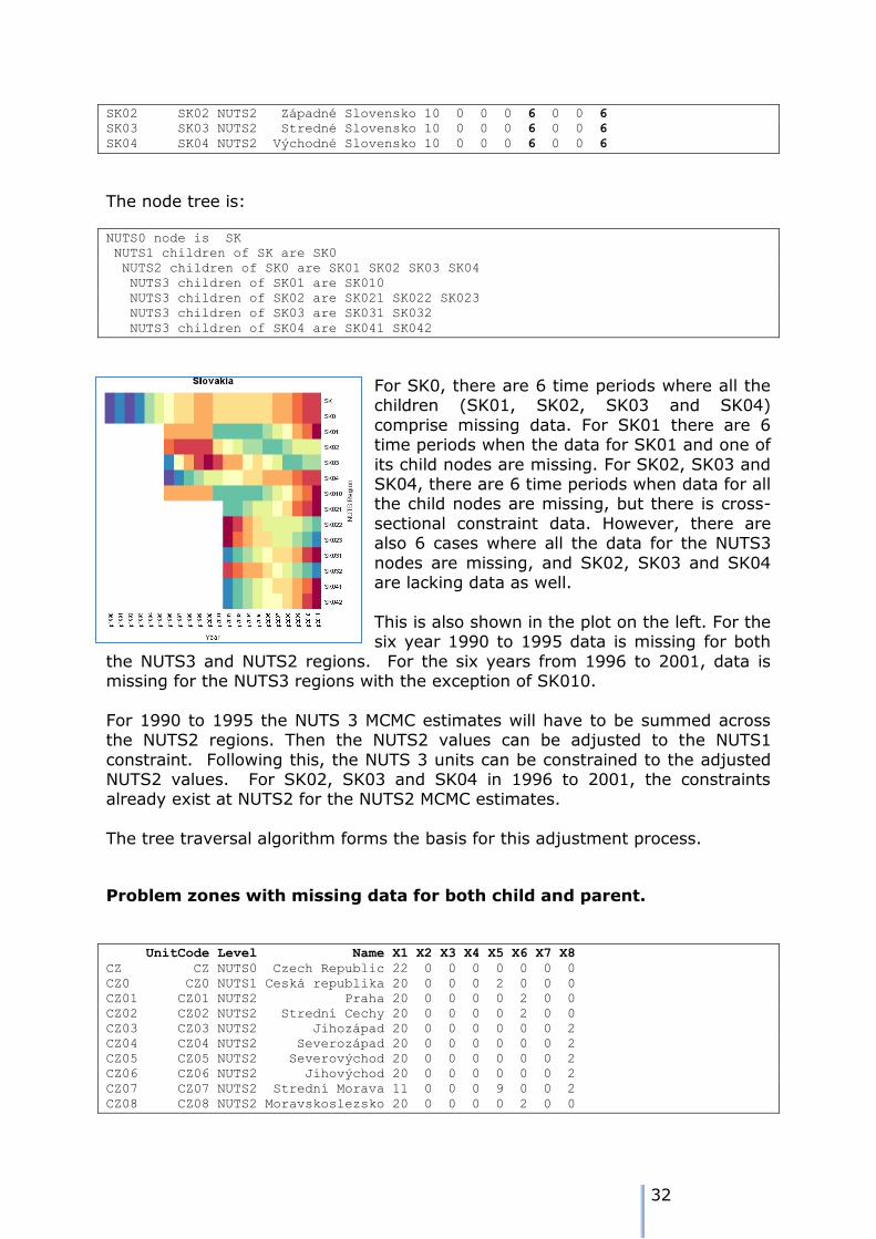
SK02 SK02 NUTS2 Západné Slovensko 10 0 0 0 6 0 0 6
SK03 SK03 NUTS2 Stredné Slovensko 10 0 0 0 6 0 0 6
SK04 SK04 NUTS2 Východné Slovensko 10 0 0 0 6 0 0 6
The node tree is:
NUTS0 node is SK
NUTS1 children of SK are SK0
NUTS2 children of SK0 are SK01 SK02 SK03 SK04
NUTS3 children of SK01 are SK010
NUTS3 children of SK02 are SK021 SK022 SK023
NUTS3 children of SK03 are SK031 SK032
NUTS3 children of SK04 are SK041 SK042
For SK0, there are 6 time periods where all the children (SK01, SK02, SK03 and SK04)
comprise missing data. For SK01 there are 6 time periods when the data for SK01 and one of
its child nodes are missing. For SK02, SK03 and SK04, there are 6 time periods when data for all the child nodes are missing, but there is cross-
sectional constraint data. However, there are also 6 cases where all the data for the NUTS3
nodes are missing, and SK02, SK03 and SK04 are lacking data as well.
This is also shown in the plot on the left. For the six year 1990 to 1995 data is missing for both
the NUTS3 and NUTS2 regions. For the six years from 1996 to 2001, data is missing for the NUTS3 regions with the exception of SK010.
For 1990 to 1995 the NUTS 3 MCMC estimates will have to be summed across the NUTS2 regions. Then the NUTS2 values can be adjusted to the NUTS1
constraint. Following this, the NUTS 3 units can be constrained to the adjusted NUTS2 values. For SK02, SK03 and SK04 in 1996 to 2001, the constraints already exist at NUTS2 for the NUTS2 MCMC estimates.
The tree traversal algorithm forms the basis for this adjustment process.
Problem zones with missing data for both child and parent.
UnitCode Level Name X1 X2 X3 X4 X5 X6 X7 X8
CZ CZ NUTS0 Czech Republic 22 0 0 0 0 0 0 0
CZ0 CZ0 NUTS1 Ceská republika 20 0 0 0 2 0 0 0
CZ01 CZ01 NUTS2 Praha 20 0 0 0 0 2 0 0
CZ02 CZ02 NUTS2 Strední Cechy 20 0 0 0 0 2 0 0
CZ03 CZ03 NUTS2 Jihozápad 20 0 0 0 0 0 0 2
CZ04 CZ04 NUTS2 Severozápad 20 0 0 0 0 0 0 2
CZ05 CZ05 NUTS2 Severovýchod 20 0 0 0 0 0 0 2
CZ06 CZ06 NUTS2 Jihovýchod 20 0 0 0 0 0 0 2
CZ07 CZ07 NUTS2 Strední Morava 11 0 0 0 9 0 0 2
CZ08 CZ08 NUTS2 Moravskoslezsko 20 0 0 0 0 2 0 0

33
UnitCode Level Name X1 X2 X3 X4 X5 X6 X7 X8
DE4 DE4 NUTS1 Brandenburg 17 0 0 0 5 0 0 0
DE41 DE41 NUTS2 Brandenburg - Nordost 16 0 0 0 1 0 0 5
DE42 DE42 NUTS2 Brandenburg - Südwest 16 0 0 0 1 0 0 5
DED1 DED1 NUTS2 Chemnitz 15 0 0 0 2 0 0 5
DED2 DED2 NUTS2 Dresden 16 0 0 0 1 0 0 5
DED3 DED3 NUTS2 Leipzig 15 0 0 0 2 0 0 5
UnitCode Level Name X1 X2 X3 X4 X5 X6 X7 X8
DK DK NUTS0 Denmark 22 0 0 0 0 0 0 0
DK0 DK0 NUTS1 Danmark 5 0 0 0 17 0 0 0
DK01 DK01 NUTS2 Hovedstaden 5 0 0 0 0 0 17 0
DK02 DK02 NUTS2 Sjælland 5 0 0 0 0 0 0 17
DK03 DK03 NUTS2 Syddanmark 5 0 0 0 0 17 0 0
DK04 DK04 NUTS2 Midtjylland 5 0 0 0 0 0 0 17
DK05 DK05 NUTS2 Nordjylland 5 0 0 0 0 17 0 0
UnitCode Level Name X1 X2 X3 X4 X5 X6 X7 X8
HR HR NUTS0 Croatia 22 0 0 0 0 0 0 0
HR0 HR0 NUTS1 Hrvatska 11 0 0 0 11 0 0 0
HR01 HR01 NUTS2 Sjeverozapadna Hrvatska 11 1 0 0 0 0 0 10
HR02 HR02 NUTS2 Sredisnja i Istocna (Panonska) Hrvatska 11 1 0 0 0 0 0 10
HR03 HR03 NUTS2 Jadranska Hrvatska 11 1 0 0 0 0 0 10
UnitCode Level Name X1 X2 X3 X4 X5 X6 X7 X8
IE IE NUTS0 Ireland 22 0 0 0 0 0 0 0
IE0 IE0 NUTS1 Éire/Ireland 15 0 0 0 7 0 0 0
IE01 IE01 NUTS2 Border, Midland and Western 5 0 0 0 10 0 0 7
IE02 IE02 NUTS2 Southern and Eastern 5 0 0 0 10 0 0 7
UnitCode Level Name X1 X2 X3 X4 X5 X6 X7 X8
PL PL NUTS0 Poland 21 0 0 0 1 0 0 0
PL1 PL1 NUTS1 Region Centralny 21 0 0 0 0 0 0 1
PL2 PL2 NUTS1 Region Poludniowy 21 0 0 0 0 0 0 1
PL3 PL3 NUTS1 Region Wschodni 21 0 0 0 0 0 0 1
PL4 PL4 NUTS1 Region Pólnocno-Zachodni 21 0 0 0 0 0 0 1
PL5 PL5 NUTS1 Region Poludniowo-Zachodni 21 0 0 0 0 0 0 1
PL6 PL6 NUTS1 Region Pólnocny 21 0 0 0 0 0 0 1
PL11 PL11 NUTS2 Lódzkie 11 0 0 0 10 0 0 1
PL12 PL12 NUTS2 Mazowieckie 11 0 0 0 10 0 0 1
PL21 PL21 NUTS2 Malopolskie 11 0 0 0 10 0 0 1
PL22 PL22 NUTS2 Slaskie 11 0 0 0 10 0 0 1
PL31 PL31 NUTS2 Lubelskie 11 0 0 0 10 0 0 1
PL32 PL32 NUTS2 Podkarpackie 11 0 0 0 10 0 0 1
PL33 PL33 NUTS2 Swietokrzyskie 11 0 0 0 10 0 0 1
PL34 PL34 NUTS2 Podlaskie 11 0 0 0 10 0 0 1
PL41 PL41 NUTS2 Wielkopolskie 11 0 0 0 10 0 0 1
PL42 PL42 NUTS2 Zachodniopomorskie 11 0 0 0 10 0 0 1
PL43 PL43 NUTS2 Lubuskie 11 0 0 0 10 0 0 1
PL51 PL51 NUTS2 Dolnoslaskie 11 0 0 0 10 0 0 1
PL52 PL52 NUTS2 Opolskie 11 0 0 0 10 0 0 1
PL61 PL61 NUTS2 Kujawsko-Pomorskie 11 0 0 0 10 0 0 1
PL62 PL62 NUTS2 Warminsko-Mazurskie 11 0 0 0 10 0 0 1
PL63 PL63 NUTS2 Pomorskie 11 0 0 0 10 0 0 1
UnitCode Level Name X1 X2 X3 X4 X5 X6 X7 X8
PT PT NUTS0 Portugal 16 0 0 0 2 4 0 0
PT1 PT1 NUTS1 Continente 16 4 0 0 0 0 0 2
PT2 PT2 NUTS1 Região Autónoma dos Açores (PT) 20 0 0 0 0 2 0 0
PT3 PT3 NUTS1 Região Autónoma da Madeira (PT) 20 0 0 0 0 2 0 0
PT11 PT11 NUTS2 Norte 20 0 0 0 0 0 0 2
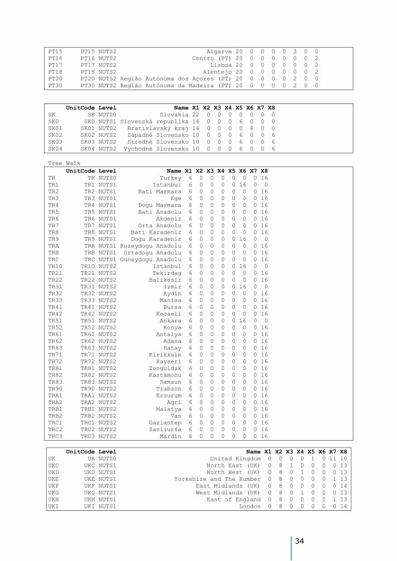
34
PT15 PT15 NUTS2 Algarve 20 0 0 0 0 2 0 0
PT16 PT16 NUTS2 Centro (PT) 20 0 0 0 0 0 0 2
PT17 PT17 NUTS2 Lisboa 20 0 0 0 0 0 0 2
PT18 PT18 NUTS2 Alentejo 20 0 0 0 0 0 0 2
PT20 PT20 NUTS2 Região Autónoma dos Açores (PT) 20 0 0 0 0 2 0 0
PT30 PT30 NUTS2 Região Autónoma da Madeira (PT) 20 0 0 0 0 2 0 0
UnitCode Level Name X1 X2 X3 X4 X5 X6 X7 X8
SK SK NUTS0 Slovakia 22 0 0 0 0 0 0 0
SK0 SK0 NUTS1 Slovenská republika 16 0 0 0 6 0 0 0
SK01 SK01 NUTS2 Bratislavský kraj 16 0 0 0 0 6 0 0
SK02 SK02 NUTS2 Západné Slovensko 10 0 0 0 6 0 0 6
SK03 SK03 NUTS2 Stredné Slovensko 10 0 0 0 6 0 0 6
SK04 SK04 NUTS2 Východné Slovensko 10 0 0 0 6 0 0 6
Tree Walk
UnitCode Level Name X1 X2 X3 X4 X5 X6 X7 X8
TR TR NUTS0 Turkey 6 0 0 0 0 0 0 16
TR1 TR1 NUTS1 Istanbul 6 0 0 0 0 16 0 0
TR2 TR2 NUTS1 Bati Marmara 6 0 0 0 0 0 0 16
TR3 TR3 NUTS1 Ege 6 0 0 0 0 0 0 16
TR4 TR4 NUTS1 Dogu Marmara 6 0 0 0 0 0 0 16
TR5 TR5 NUTS1 Bati Anadolu 6 0 0 0 0 0 0 16
TR6 TR6 NUTS1 Akdeniz 6 0 0 0 0 0 0 16
TR7 TR7 NUTS1 Orta Anadolu 6 0 0 0 0 0 0 16
TR8 TR8 NUTS1 Bati Karadeniz 6 0 0 0 0 0 0 16
TR9 TR9 NUTS1 Dogu Karadeniz 6 0 0 0 0 16 0 0
TRA TRA NUTS1 Kuzeydogu Anadolu 6 0 0 0 0 0 0 16
TRB TRB NUTS1 Ortadogu Anadolu 6 0 0 0 0 0 0 16
TRC TRC NUTS1 Güneydogu Anadolu 6 0 0 0 0 0 0 16
TR10 TR10 NUTS2 Istanbul 6 0 0 0 0 16 0 0
TR21 TR21 NUTS2 Tekirdag 6 0 0 0 0 0 0 16
TR22 TR22 NUTS2 Balikesir 6 0 0 0 0 0 0 16
TR31 TR31 NUTS2 Izmir 6 0 0 0 0 16 0 0
TR32 TR32 NUTS2 Aydin 6 0 0 0 0 0 0 16
TR33 TR33 NUTS2 Manisa 6 0 0 0 0 0 0 16
TR41 TR41 NUTS2 Bursa 6 0 0 0 0 0 0 16
TR42 TR42 NUTS2 Kocaeli 6 0 0 0 0 0 0 16
TR51 TR51 NUTS2 Ankara 6 0 0 0 0 16 0 0
TR52 TR52 NUTS2 Konya 6 0 0 0 0 0 0 16
TR61 TR61 NUTS2 Antalya 6 0 0 0 0 0 0 16
TR62 TR62 NUTS2 Adana 6 0 0 0 0 0 0 16
TR63 TR63 NUTS2 Hatay 6 0 0 0 0 0 0 16
TR71 TR71 NUTS2 Kirikkale 6 0 0 0 0 0 0 16
TR72 TR72 NUTS2 Kayseri 6 0 0 0 0 0 0 16
TR81 TR81 NUTS2 Zonguldak 6 0 0 0 0 0 0 16
TR82 TR82 NUTS2 Kastamonu 6 0 0 0 0 0 0 16
TR83 TR83 NUTS2 Samsun 6 0 0 0 0 0 0 16
TR90 TR90 NUTS2 Trabzon 6 0 0 0 0 0 0 16
TRA1 TRA1 NUTS2 Erzurum 6 0 0 0 0 0 0 16
TRA2 TRA2 NUTS2 Agri 6 0 0 0 0 0 0 16
TRB1 TRB1 NUTS2 Malatya 6 0 0 0 0 0 0 16
TRB2 TRB2 NUTS2 Van 6 0 0 0 0 0 0 16
TRC1 TRC1 NUTS2 Gaziantep 6 0 0 0 0 0 0 16
TRC2 TRC2 NUTS2 Sanliurfa 6 0 0 0 0 0 0 16
TRC3 TRC3 NUTS2 Mardin 6 0 0 0 0 0 0 16
UnitCode Level Name X1 X2 X3 X4 X5 X6 X7 X8
UK UK NUTS0 United Kingdom 0 0 0 0 1 0 11 10
UKC UKC NUTS1 North East (UK) 0 8 1 0 0 0 0 13
UKD UKD NUTS1 North West (UK) 0 8 0 1 0 0 0 13
UKE UKE NUTS1 Yorkshire and The Humber 0 8 0 0 0 0 1 13
UKF UKF NUTS1 East Midlands (UK) 0 8 0 0 0 0 0 14
UKG UKG NUTS1 West Midlands (UK) 0 8 0 1 0 0 0 13
UKH UKH NUTS1 East of England 0 8 0 0 0 0 1 13
UKI UKI NUTS1 London 0 8 0 0 0 0 0 14
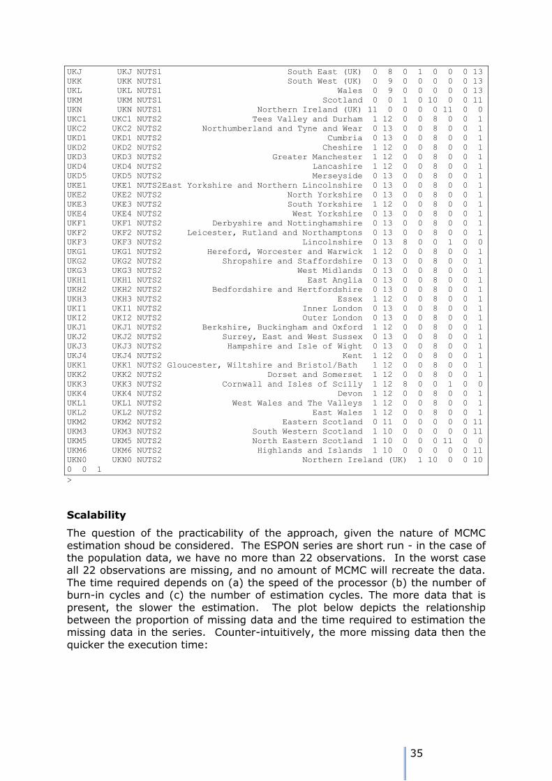
35
UKJ UKJ NUTS1 South East (UK) 0 8 0 1 0 0 0 13
UKK UKK NUTS1 South West (UK) 0 9 0 0 0 0 0 13
UKL UKL NUTS1 Wales 0 9 0 0 0 0 0 13
UKM UKM NUTS1 Scotland 0 0 1 0 10 0 0 11
UKN UKN NUTS1 Northern Ireland (UK) 11 0 0 0 0 11 0 0
UKC1 UKC1 NUTS2 Tees Valley and Durham 1 12 0 0 8 0 0 1
UKC2 UKC2 NUTS2 Northumberland and Tyne and Wear 0 13 0 0 8 0 0 1
UKD1 UKD1 NUTS2 Cumbria 0 13 0 0 8 0 0 1
UKD2 UKD2 NUTS2 Cheshire 1 12 0 0 8 0 0 1
UKD3 UKD3 NUTS2 Greater Manchester 1 12 0 0 8 0 0 1
UKD4 UKD4 NUTS2 Lancashire 1 12 0 0 8 0 0 1
UKD5 UKD5 NUTS2 Merseyside 0 13 0 0 8 0 0 1
UKE1 UKE1 NUTS2East Yorkshire and Northern Lincolnshire 0 13 0 0 8 0 0 1
UKE2 UKE2 NUTS2 North Yorkshire 0 13 0 0 8 0 0 1
UKE3 UKE3 NUTS2 South Yorkshire 1 12 0 0 8 0 0 1
UKE4 UKE4 NUTS2 West Yorkshire 0 13 0 0 8 0 0 1
UKF1 UKF1 NUTS2 Derbyshire and Nottinghamshire 0 13 0 0 8 0 0 1
UKF2 UKF2 NUTS2 Leicester, Rutland and Northamptons 0 13 0 0 8 0 0 1
UKF3 UKF3 NUTS2 Lincolnshire 0 13 8 0 0 1 0 0
UKG1 UKG1 NUTS2 Hereford, Worcester and Warwick 1 12 0 0 8 0 0 1
UKG2 UKG2 NUTS2 Shropshire and Staffordshire 0 13 0 0 8 0 0 1
UKG3 UKG3 NUTS2 West Midlands 0 13 0 0 8 0 0 1
UKH1 UKH1 NUTS2 East Anglia 0 13 0 0 8 0 0 1
UKH2 UKH2 NUTS2 Bedfordshire and Hertfordshire 0 13 0 0 8 0 0 1
UKH3 UKH3 NUTS2 Essex 1 12 0 0 8 0 0 1
UKI1 UKI1 NUTS2 Inner London 0 13 0 0 8 0 0 1
UKI2 UKI2 NUTS2 Outer London 0 13 0 0 8 0 0 1
UKJ1 UKJ1 NUTS2 Berkshire, Buckingham and Oxford 1 12 0 0 8 0 0 1
UKJ2 UKJ2 NUTS2 Surrey, East and West Sussex 0 13 0 0 8 0 0 1
UKJ3 UKJ3 NUTS2 Hampshire and Isle of Wight 0 13 0 0 8 0 0 1
UKJ4 UKJ4 NUTS2 Kent 1 12 0 0 8 0 0 1
UKK1 UKK1 NUTS2 Gloucester, Wiltshire and Bristol/Bath 1 12 0 0 8 0 0 1
UKK2 UKK2 NUTS2 Dorset and Somerset 1 12 0 0 8 0 0 1
UKK3 UKK3 NUTS2 Cornwall and Isles of Scilly 1 12 8 0 0 1 0 0
UKK4 UKK4 NUTS2 Devon 1 12 0 0 8 0 0 1
UKL1 UKL1 NUTS2 West Wales and The Valleys 1 12 0 0 8 0 0 1
UKL2 UKL2 NUTS2 East Wales 1 12 0 0 8 0 0 1
UKM2 UKM2 NUTS2 Eastern Scotland 0 11 0 0 0 0 0 11
UKM3 UKM3 NUTS2 South Western Scotland 1 10 0 0 0 0 0 11
UKM5 UKM5 NUTS2 North Eastern Scotland 1 10 0 0 0 11 0 0
UKM6 UKM6 NUTS2 Highlands and Islands 1 10 0 0 0 0 0 11
UKN0 UKN0 NUTS2 Northern Ireland (UK) 1 10 0 0 10
0 0 1
>
Scalability
The question of the practicability of the approach, given the nature of MCMC
estimation shoud be considered. The ESPON series are short run - in the case of the population data, we have no more than 22 observations. In the worst case all 22 observations are missing, and no amount of MCMC will recreate the data.
The time required depends on (a) the speed of the processor (b) the number of burn-in cycles and (c) the number of estimation cycles. The more data that is
present, the slower the estimation. The plot below depicts the relationship between the proportion of missing data and the time required to estimation the missing data in the series. Counter-intuitively, the more missing data then the
quicker the execution time:
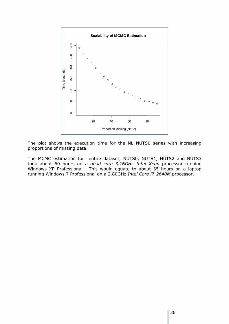
36
The plot shows the execution time for the NL NUTS0 series with increasing proportions of missing data.
The MCMC estimation for entire dataset, NUTS0, NUTS1, NUTS2 and NUTS3
took about 60 hours on a quad core 3.16GHz Intel Xeon processor running Windows XP Professional. This would equate to about 35 hours on a laptop running Windows 7 Professional on a 2.80GHz Intel Core i7-2640M processor.
20 40 60 80
05
01
00
15
02
00
25
03
00
Scalability of MCMC Estimation
Proportion Missing (N=22)
Tim
e (
se
co
nd
s)

37
5. ESPON Time series in practice
The code for the various tasks to be undertaken is included as Appendices 2, 3, 4 and 5. We can identify as number of tasks which are relevant. It should be noted that the temptation to regard the entire process as automatic should be
avoided, although much of the activity can be automated.
Getting started
Currently the organisation of the activity assumes that the R code and the data
are in the same folder. This is Time_Series_Analysis/Sandbox but the code and data can be separated. All code should be in the same folder. The relevant files are:
Modelling_and_Imputation.R
ImputeMissingData.R
tfile1.JAGS
tfile2.JAGS
The following R libraries are required: gdata
rjags
RColorBrewer
Data requires that a current version of the perl11 language is installed, and rjags requires that a current version of JAGS is installed12.
The various tasks are identified in the code, and are briefly described below.
Task 1: Data load and pre-processing
The four worksheets in the ESPON Database spreadsheet are read into four
separate data frames. We use the read.xls() function for this. Of interest are the Source and Data worksheets.
The Source worksheet is parsed to extract as list of the data providers and their
identification codes. The data frame sourceIndex needs to be examined to identify the codes for EUROSTAT and the National Statistical Agencies13.
The relevant codes are extracted to another dataframe, sourcesOK, and this is used as a filter for the data extraction. The Data worksheet is split into two data
frames which hold (a) the data and (b) the corresponding index codes. Once the non-EUROSTAT/NSA data has be filtered, the resulting data frame Data.estim, will be used in the remainder of the exercise.
11 Perl can be downloaded from http://www.activestate.com/activeperl/downloads 12 JAGS can be installed from http://sourceforge.net/projects/mcmc-jags/files/ 13 The data as supplied by the RIATE team contains original data as well as RIATE's own
estimations of the missing data

38
As a final activity under this task the rows in Data.estim are index by their
corresponding NUTS codes. This indexing is central to the spatial coherence activity described in a later task.
Task 2: Missing data pattern analysis
It is important to be aware of the patterns of missing data in the dataset. This gives an overall picture of the patterns in each country, and also an indication of
the scale of the problem. A useful tool for this purpose is the heatmap. The columns in the heatmap
represent the individual time periods, and the rows represent the NUTS regions. A separate heatmap can be produced for each country. Data values are colour
coded according to their value, so some broad indications of the range of values and the trends in each group of series can be obtained from the heatmap.
The heatmap() function has a number of options, including the re-ordering of the rows and columns as a result of the application of hierarchical clustering.
These options are turned off: (Colv=NA, Rowv=NA). The cells in the heatmap which arise from the intersection of a year and a NUTS region with missing data
are coloured grey. The resulting heatmaps are included as separate plots in Appendix 7.
Task 3: Missing data at NUTS0/1/2
Ensuribng spatial coherence is an important issue for the imputation process. This requires reliable control data for the higher NUTS levels. Inevitably, there
will need to be consistent series for the NUTS0 level. Task 3 involves an enurmation of NUTS0/1/2 regions with missing data. The complete.cases()
function is used to identify NUTS regions with missing data. These are listed.
Task 4: exploring general patterns
Analysis of the series suggested that an simple linear or exponential trend model
might be insufficient to capture the overall trend pattern. Eventually it was decided that a quadratic term would be added to the model. If the empirical trend was more or less linear, then the coefficient on the quadratic term would
be close to zero. Four plots are shown below for Austria, France, Netherlands, and Slovenia:
The non-missing data points A line or lines connecting the non-missing data points
A line to show linear trend A line to shown quadratic trend
Whilst the general pattern is modelled well by the linear term, the fit is improved by the quadratic term – very noticeably in the case of Slovenia.

39
Task 5: extraction of the data for a single country
Much of the development work took place using the data series for NUTS regions of Austria as an example. The code under Task 5 shows how to extract data for
a single country for further analysis. It also shows how to create a backlink in the spatial hierarchy, so that the
'parent' region for each NUTS region can be identified.
In the normal course of events, this code section need not be used, although it is helpful to have it for testing and debugging purposes.
Task 6: MCMC estimation
1990 1995 2000 2005 2010
7800000
8200000
Austria
Year
Popula
tion
1990 1995 2000 2005 2010
5.8
e+
07
6.1
e+
07
6.4
e+
07
France
Year
Popula
tion
1990 1995 2000 2005 2010
15000000
16000000
Netherlands
Year
Popula
tion
1990 1995 2000 2005 2010
1980000
2010000
2040000
Slovenia
Year
Popula
tion

40
The central task of the exercise is to estimate the missing data in each series using Markov Chain Monte Carlo methods. The main function which organises
the data into input for JAGS, ImputeMissingData(), is shown and commented in Appendix 3.
All rows with missing in Data.estim can be estimated with the exception of any row with fewer than 3 observations.
The estimation takes place in a loop, whose start/end locations are controlled by
the variables startrow and endrow. In the code these are set to 1 and the number of rows in Data.estim. This task is massively time consuming, and if there is doubt that the computer on which the process is run would stay up, then
the estimation could be subdivided.
Once the missing data in a NUTS region has been estimated and the row written to the output matrix, NUTSData.completed, it is not referenced again until Task 6 has completed.
The final step in the Task is to write the intermediate results to a file. The
estimation of all the missing data for 1990-2001 for all NUTS0/1/2/3 regions took some 60 hours on a 2.8GHz Intel Core i7-260M processor, so some
precautions are needed to ensure that the task does not have be repeated too many times. Should there be a system failure when the last few estimations are to be completed would be extremely unfortunate, so writing out the intermediate
results every 100 or so iterations would be sensible.
The JAGS code appears to be robust – only one series caused a failure, and that was one in which all values were missing.
Task 6A: Scalability assessment
Task 6a can be omitted – it is present only to allow an assessment of the scalbiluty of the process, using data from the Netherlands as an example. The plot from this Task appears on page 36.
Task 7: Spatial Coherence Adjustment
One of the most challenging parts of the work has been to develop an algorithm which permits adjustment of lower level NUTS estimations to constraining values
at the higher NUTS levels. There are two subtasks.
Task 7a is a manual fix for Portugal. PT is missing years 1992 and 1995. PT1 is missing the same years. However, the NUTS2 regions in PT1 are present. The manual fix is to sum the PT1* regions to PT1, and then PT1+PT2+PT3 to PT.
This could be automated, but analysis of other series would be needed to determine whether it is a more widespread problem. The code for the manual
fix is present, and therefore is reproducible14.
14 Reproducibility is science is the ability of an enture study to be reproduced by either the researcher themselves, or by an independent third party. See also Buckheit JB and

41
Task 7b includes the coherence algorithm. This is presented as a function
ConstrainTotals2() which takes the missing data pattern data frame, the data frame of unadjusted estimates, and then range of data columns to be adjusted.
The output is a spatially coherent data frame of actual data and estimates. The algorithm is a top down algorithm. The indexing of the rows by their NUTS
code means that it is possible to identify the parent region (the NUTS chode is one character shorter). NUTS1 regions are first constrained to the NUTS0 values
– with care being taken when only a subset of these has been estimated. The hierarchical relationship between the NUTS levels, and the existence of the 'parent' vector means that this can be coded in a loop.
Once the NUTS1 regions have been constrained, the NUTS2 region estimates can be constrained to the NUTS1 totals. Finally the NUTS3 region estimates can be constrained to the NUTS2 totals.
The resulting data frame can be output to a file if required.
Other functions
CheckCountry(): this uses the function CheckConstraint() – lists the children for each parent node in the tree
CheckTree(): traverses the tree in order
CheckMissingPattern(): examines the missing data patterns for each parent node.
In the final section are some plots of random numbers drawn in samples of different sizes for different distributions (normal, gamma, beta, multivariate
normal), together with random normal for different precisions and a non-informative prior to show the influence of increasing the sample size on the estimates of the mean.
Donoho, 1995, WaveLab and Reproducible Research, Dept. of Statistics, Stanford University, Tech. Rep. 474
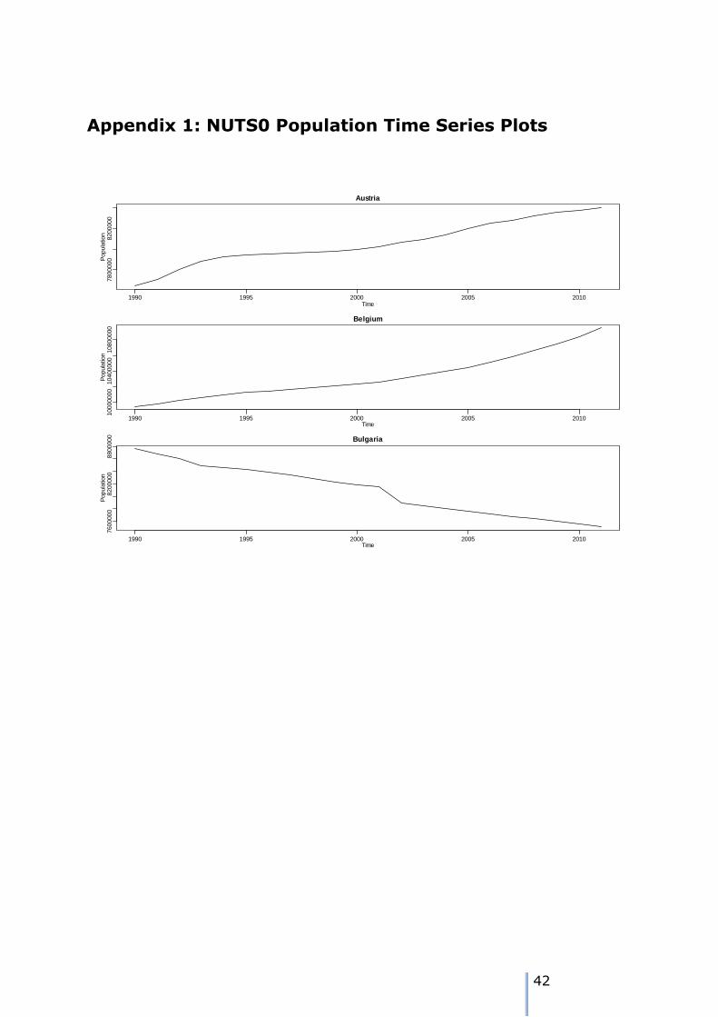
42
Appendix 1: NUTS0 Population Time Series Plots
Austria
Time
Popula
tion
1990 1995 2000 2005 2010
7800000
8200000
Belgium
Time
Popula
tion
1990 1995 2000 2005 2010
10000000
10400000
10800000
Bulgaria
Time
Popula
tion
1990 1995 2000 2005 2010
7600000
8200000
8800000
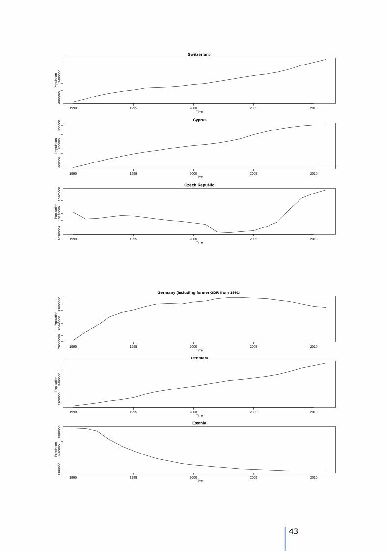
43
Switzerland
Time
Popula
tion
1990 1995 2000 2005 2010
6800000
7400000
Cyprus
Time
Popula
tion
1990 1995 2000 2005 2010
600000
700000
800000
Czech Republic
Time
Popula
tion
1990 1995 2000 2005 201010200000
10350000
10500000
Germany (including former GDR from 1991)
Time
Popula
tion
1990 1995 2000 2005 201079000000
80500000
82000000
Denmark
Time
Popula
tion
1990 1995 2000 2005 2010
5200000
5400000
Estonia
Time
Popula
tion
1990 1995 2000 2005 2010
1350000
1450000
1550000
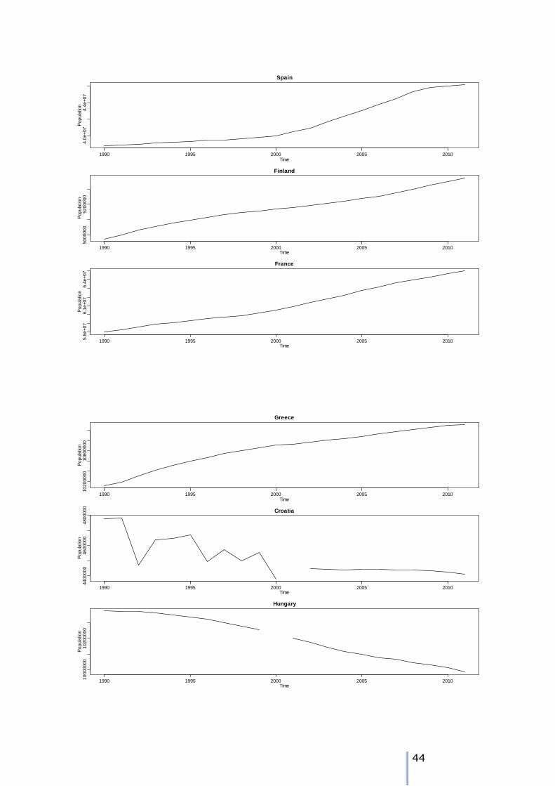
44
Spain
Time
Popula
tion
1990 1995 2000 2005 2010
4.0
e+07
4.4
e+07
Finland
Time
Popula
tion
1990 1995 2000 2005 2010
5000000
5200000
France
Time
Popula
tion
1990 1995 2000 2005 2010
5.8
e+07
6.1
e+07
6.4
e+07
Greece
Time
Popula
tion
1990 1995 2000 2005 2010
10200000
10800000
Croatia
Time
Popula
tion
1990 1995 2000 2005 2010
4400000
4600000
4800000
Hungary
Time
Popula
tion
1990 1995 2000 2005 2010
10000000
10200000
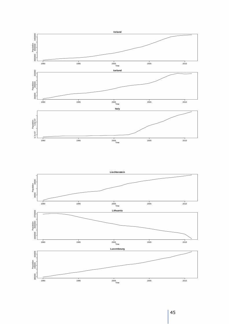
45
Ireland
Time
Popula
tion
1990 1995 2000 2005 2010
3600000
4000000
4400000
Iceland
Time
Popula
tion
1990 1995 2000 2005 2010
260000
290000
320000
Italy
Time
Popula
tion
1990 1995 2000 2005 2010
5.7
e+07
5.9
e+07
Liechtenstein
Time
Popula
tion
1990 1995 2000 2005 2010
30000
34000
Lithuania
Time
Popula
tion
1990 1995 2000 2005 2010
3300000
3500000
3700000
Luxembourg
Time
Popula
tion
1990 1995 2000 2005 2010
380000
440000
500000
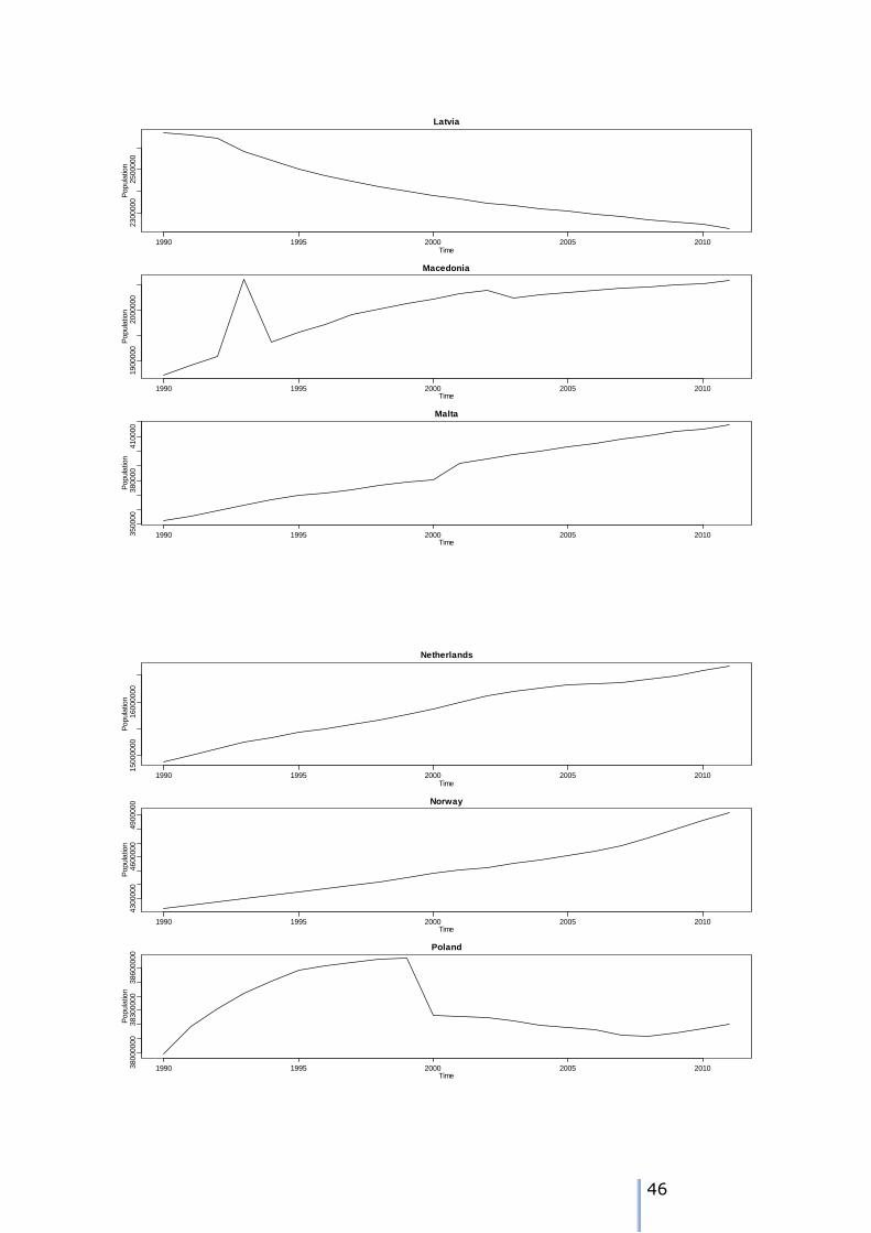
46
Latvia
Time
Popula
tion
1990 1995 2000 2005 2010
2300000
2500000
Macedonia
Time
Popula
tion
1990 1995 2000 2005 2010
1900000
2000000
Malta
Time
Popula
tion
1990 1995 2000 2005 2010350000
380000
410000
Netherlands
Time
Popula
tion
1990 1995 2000 2005 2010
15000000
16000000
Norway
Time
Popula
tion
1990 1995 2000 2005 2010
4300000
4600000
4900000
Poland
Time
Popula
tion
1990 1995 2000 2005 201038000000
38300000
38600000
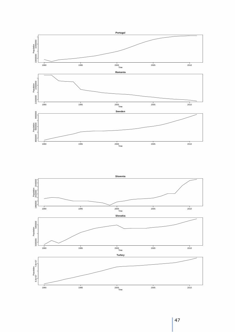
47
Portugal
Time
Popula
tion
1990 1995 2000 2005 2010
10000000
10400000
Romania
Time
Popula
tion
1990 1995 2000 2005 2010
21500000
22500000
Sweden
Time
Popula
tion
1990 1995 2000 2005 2010
8600000
9000000
9400000
Slovenia
Time
Popula
tion
1990 1995 2000 2005 2010
1980000
2010000
2040000
Slovakia
Time
Popula
tion
1990 1995 2000 2005 2010
5300000
5400000
Turkey
Time
Popula
tion
1990 1995 2000 2005 2010
6.0
e+07
7.0
e+07

48
United Kingdom
Time
Popula
tion
1990 1995 2000 2005 2010
5.8
e+07
6.0
e+07
6.2
e+07

49
Appendix 2: Main analysis and imputation R functions
################################################################################
#######################################################################
###### V5
#
# ESPON M4D Multidimensional Database Design and Development
#
# Time Series Estimation
#
# Data Exploration, Estimation, and Coherence functions
#
#
### Authors:
#
# Martin Charlton and Chris Brunsdon
#
### Address:
#
# National Centre for Geocomputation
# National University of Ireland, Maynooth
# Maynooth, Co Kildare, IRELAND
#
# V1.01: June 2014
#
#### (c) ESPON
#
# Code is made avilable under the GNU GENERAL PUBLIC LICENSE, Version 3
# Text of the License is at http://www.gnu.org/licenses/gpl.txt
#
#######################################################################
#########
#######################################################################
#########
###
### Identify a working folder - all data/software in in this folder
###
dsn <- "F:\\Time_Series_Analysis\\Sandbox" # Data stick
setwd(dsn)
###
### Load the libraries needed for the analysis and estimation
###
require(RColorBrewer)
require(gdata)
require(rjags)
#######################################################################
##########
### TASK 1: Read the data, identify the EUROSTAT/NSA data and split
data
### and source indices into separate worksheets

50
#######################################################################
##########
Dataset <- read.xls(paste(dsn,"\\M4D_poptot1990-
2011_20120522.xls",sep=""), sheet=1,header=FALSE)
Indicator <- read.xls(paste(dsn,"\\M4D_poptot1990-
2011_20120522.xls",sep=""), sheet=2,header=FALSE)
Source <- read.xls(paste(dsn,"\\M4D_poptot1990-
2011_20120522.xls",sep=""), sheet=3,header=FALSE)
Data <- read.xls(paste(dsn,"\\M4D_poptot1990-
2011_20120522.xls",sep=""), sheet=4,header=FALSE)
###
### Parse the 'Source' worksheet for the provider index codes and names
###
len3 <- dim(Source)[1]
sourceLabels <- which(Source[,1] == "Label")
sourceProvider <- which(Source[,1] == "Provider")
sourceIndex <-
data.frame(Source[sourceLabels,2],Source[sourceProvider,3])
colnames(sourceIndex) <- c("Label","Provider")
sourceIndex
#############################################
sourcesOK <- sourceIndex[c(1:32),] # These are the rows for which
data is from
# EUROSTAT + Nation al Statistical
Agencies
#############################################
###
### Split 'Data' worksheet into '.data' and '.source' worksheets
###
len2 <- dim(Data)[1] # number
of rows
dataCols <- seq(5,47,2) # columns
with data
Data.data <- Data[4:len2,c(1,2,4,dataCols)] # data
Data.source <- Data[4:len2,c(1,2,4,dataCols+1)] # source
information
colnames(Data.data) <-
c("UnitCode","Level","Name",paste("p",1990:2011,sep=""))
colnames(Data.source) <-
c("UnitCode","Level","Name",paste("s",1990:2011,sep=""))
###
### Create data frame 'Data.estim' which we used as the basis for
subsequent estimation
###
as.numeric.factor <- function(x) {as.numeric(levels(x))[x]} #
convert factors to numeric
Data.estim <- Data.data # Copy
old -> new
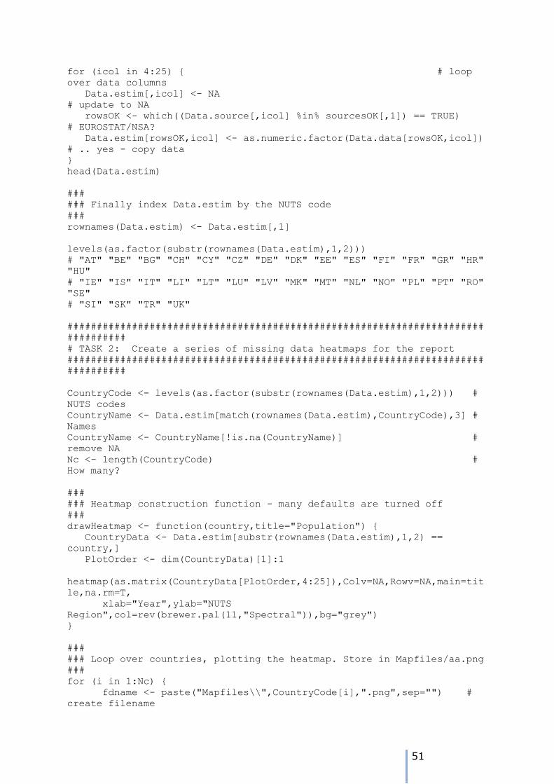
51
for (icol in 4:25) { # loop
over data columns
Data.estim[,icol] <- NA
# update to NA
rowsOK <- which((Data.source[,icol] %in% sourcesOK[,1]) == TRUE)
# EUROSTAT/NSA?
Data.estim[rowsOK,icol] <- as.numeric.factor(Data.data[rowsOK,icol])
# .. yes - copy data
}
head(Data.estim)
###
### Finally index Data.estim by the NUTS code
###
rownames(Data.estim) <- Data.estim[,1]
levels(as.factor(substr(rownames(Data.estim),1,2)))
# "AT" "BE" "BG" "CH" "CY" "CZ" "DE" "DK" "EE" "ES" "FI" "FR" "GR" "HR"
"HU"
# "IE" "IS" "IT" "LI" "LT" "LU" "LV" "MK" "MT" "NL" "NO" "PL" "PT" "RO"
"SE"
# "SI" "SK" "TR" "UK"
#######################################################################
##########
# TASK 2: Create a series of missing data heatmaps for the report
#######################################################################
##########
CountryCode <- levels(as.factor(substr(rownames(Data.estim),1,2))) #
NUTS codes
CountryName <- Data.estim[match(rownames(Data.estim),CountryCode),3] #
Names
CountryName <- CountryName[!is.na(CountryName)] #
remove NA
Nc <- length(CountryCode) #
How many?
###
### Heatmap construction function - many defaults are turned off
###
drawHeatmap <- function(country,title="Population") {
CountryData <- Data.estim[substr(rownames(Data.estim),1,2) ==
country,]
PlotOrder <- dim(CountryData)[1]:1
heatmap(as.matrix(CountryData[PlotOrder,4:25]),Colv=NA,Rowv=NA,main=tit
le,na.rm=T,
xlab="Year",ylab="NUTS
Region",col=rev(brewer.pal(11,"Spectral")),bg="grey")
}
###
### Loop over countries, plotting the heatmap. Store in Mapfiles/aa.png
###
for (i in 1:Nc) {
fdname <- paste("Mapfiles\\",CountryCode[i],".png",sep="") #
create filename
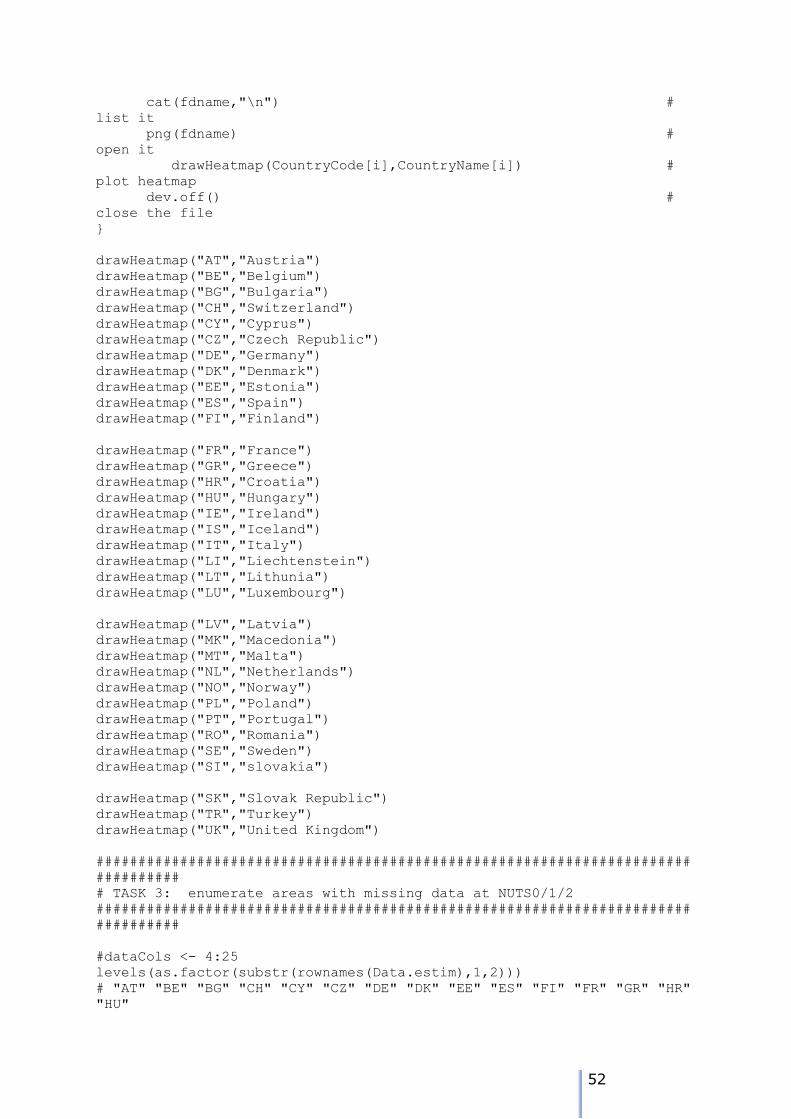
52
cat(fdname,"\n") #
list it
png(fdname) #
open it
drawHeatmap(CountryCode[i],CountryName[i]) #
plot heatmap
dev.off() #
close the file
}
drawHeatmap("AT","Austria")
drawHeatmap("BE","Belgium")
drawHeatmap("BG","Bulgaria")
drawHeatmap("CH","Switzerland")
drawHeatmap("CY","Cyprus")
drawHeatmap("CZ","Czech Republic")
drawHeatmap("DE","Germany")
drawHeatmap("DK","Denmark")
drawHeatmap("EE","Estonia")
drawHeatmap("ES","Spain")
drawHeatmap("FI","Finland")
drawHeatmap("FR","France")
drawHeatmap("GR","Greece")
drawHeatmap("HR","Croatia")
drawHeatmap("HU","Hungary")
drawHeatmap("IE","Ireland")
drawHeatmap("IS","Iceland")
drawHeatmap("IT","Italy")
drawHeatmap("LI","Liechtenstein")
drawHeatmap("LT","Lithunia")
drawHeatmap("LU","Luxembourg")
drawHeatmap("LV","Latvia")
drawHeatmap("MK","Macedonia")
drawHeatmap("MT","Malta")
drawHeatmap("NL","Netherlands")
drawHeatmap("NO","Norway")
drawHeatmap("PL","Poland")
drawHeatmap("PT","Portugal")
drawHeatmap("RO","Romania")
drawHeatmap("SE","Sweden")
drawHeatmap("SI","slovakia")
drawHeatmap("SK","Slovak Republic")
drawHeatmap("TR","Turkey")
drawHeatmap("UK","United Kingdom")
#######################################################################
##########
# TASK 3: enumerate areas with missing data at NUTS0/1/2
#######################################################################
##########
#dataCols <- 4:25
levels(as.factor(substr(rownames(Data.estim),1,2)))
# "AT" "BE" "BG" "CH" "CY" "CZ" "DE" "DK" "EE" "ES" "FI" "FR" "GR" "HR"
"HU"

53
# "IE" "IS" "IT" "LI" "LT" "LU" "LV" "MK" "MT" "NL" "NO" "PL" "PT" "RO"
"SE"
# "SI" "SK" "TR" "UK"
###
### Area code/name information as in TASK 2:
###
CountryCode <- levels(as.factor(substr(rownames(Data.estim),1,2)))
CountryName <- Data.estim[match(rownames(Data.estim),CountryCode),3]
CountryName <- CountryName[!is.na(CountryName)]
NUTSlevel <- nchar(rownames(Data.estim))-2
Nc <- length(CountryCode) #
Countries
Nr <- nrow(Data.estim) #
NUTS regions
for (i in 1:Nr) { #
Loop over NUTS codes
if(NUTSlevel[i] <= 2) {
if (!complete.cases(Data.estim[i,4:25])) { #
Complete case?
nCode <- as.character(Data.estim[i,1]) #
... no, get code
nName <- as.character(Data.estim[i,3]) #
... get name
cat("Missing data for ",nCode,nName,"\n") #
... and report
}
}
}
}
#######################################################################
##########################
### Task 4: Example plots to explore general patterns in the data
#######################################################################
##########################
CountryCode <- levels(as.factor(substr(rownames(Data.estim),1,2)))
year <- 1:22
yearsq <- year^2
###
### Each plot has: base data as dots and a line in grey
### fit from a linear model in lightblue
### fit from the quadratic model in red
###
par(mfrow=c(2,2))
Popdata <- as.numeric(Data.estim["AT",4:25])
plot(1990:2011,Popdata,xlab="Year",ylab="Population",main="Austria",pch
=16,col="grey")
lines(1990:2011,Popdata,col="grey")
lines(1990:2011,(cbind(1,year) %*%
coef(lm(Popdata~year))),col="lightblue")

54
lines(1990:2011,(cbind(1,year,yearsq) %*%
coef(lm(Popdata~year+yearsq))),col="red")
Popdata <- as.numeric(Data.estim["FR",4:25])
plot(1990:2011,Popdata,xlab="Year",ylab="Population",main="France",pch=
16,col="grey")
lines(1990:2011,Popdata,col="grey")
lines(1990:2011,(cbind(1,year) %*%
coef(lm(Popdata~year))),col="lightblue")
lines(1990:2011,(cbind(1,year,yearsq) %*%
coef(lm(Popdata~year+yearsq))),col="red")
Popdata <- as.numeric(Data.estim["NL",4:25])
plot(1990:2011,Popdata,xlab="Year",ylab="Population",main="Netherlands"
,pch=16,col="grey")
lines(1990:2011,Popdata,col="grey")
lines(1990:2011,(cbind(1,year) %*%
coef(lm(Popdata~year))),col="lightblue")
lines(1990:2011,(cbind(1,year,yearsq) %*%
coef(lm(Popdata~year+yearsq))),col="red")
Popdata <- as.numeric(Data.estim["SI",4:25])
plot(1990:2011,Popdata,xlab="Year",ylab="Population",main="Slovenia",pc
h=16,col="grey")
lines(1990:2011,Popdata,col="grey")
lines(1990:2011,(cbind(1,year) %*%
coef(lm(Popdata~year))),col="lightblue")
lines(1990:2011,(cbind(1,year,yearsq) %*%
coef(lm(Popdata~year+yearsq))),col="red")
par(mfrow=c(1,1))
#######################################################################
##########################
### TASK 5: Extract data for Austria as test data *** *** *** ONLY FOR
TESTING *** *** ***
#######################################################################
##########################
Austria <- Data.estim[substr(rownames(Data.estim),1,2) == "AT",]
PlotOrder <- dim(Austria)[1]:1 #
reverse order for the heatmap
heatmap(as.matrix(Austria[PlotOrder,4:25]),Colv=NA,Rowv=NA,main="Austri
a EUROSTAT Population Data",
xlab="Year",ylab="NUTS Region",col=rev(brewer.pal(11,"Spectral")))
parent <- substr(rownames(Austria),1,nchar(rownames(Austria))-1)
parent[1] <- ""
NUTS <- rownames(Austria)
NUTS0 <- which(nchar(rownames(Austria)) == 2)
NUTS1 <- which(nchar(rownames(Austria)) == 3)
NUTS2 <- which(nchar(rownames(Austria)) == 4)
NUTS3 <- which(nchar(rownames(Austria)) == 5)

55
Data.estim <- Austria
#######################################################################
############
#### TASK 6: MCMC estimation of NUTS levels 3 series
#######################################################################
############
# Estimation loop one iteration is about 1.7 minutes for 12 missing
from 22 on
# a Intel Xeon X5460 quad core 3.16GHz processor running Windows XP
Professional
#
# 35 zones for Austria takes about an hour. As a ball park estimate,
the whole of
# Europe should take about 36 hours of computing.
#
# On an Intel Core i7-2640M processor running at 2.80Ghz it's under a
minute per fit.
# This is a 64 bit system running Windows 7 Professional. Austria would
take just
# over 30 minutes so about 18 hours for Europe.
# NUTS3 tool 199418.4 seconds 55h 24m, say ~55.5h
#
#######################################################################
###########
###
### Load the function definition
###
source("ImputeMissingData.R")
###
### Copy start data
###
NUTSData.completed <- Data.estim
nrow <- dim(Data.estim)[1] # number of
regions
NUTS <- rownames(Data.estim) # NUTS codes
NUTSlevel <- nchar(NUTS)-2 # NUTS lebels
total.time <- 0
startrow <- 1 # start at 1 ...
endrow <- nrow # ... and finish
at nrow
for (i in startrow:endrow) {
#if(NUTSlevel[i] < 3 & substr(NUTS[i],1,2) != "UK") {
if(substr(NUTS[i],1,2) != "UK") { # UK separately
if (complete.cases(Data.estim[i,4:25])) { # data complete?
cat(NUTS[i],"is complete\n") # ... yes: ignore
} else {
cat(NUTS[i],"is undergoing imputation\n") # ... no:
imputation needed
Z <- as.numeric(Data.estim[i,4:25]) # data series
Years <- 1990:2011 # time frame
for series

56
N <- length(Z) # length of
the series
missingYears <- which(is.na(Z)) # missing
observations
NM <- length(missingYears) # number of
missing obs
Scale <- 1000 # scale for
populations
tic <- proc.time()[3]
fitted.model <- ImputeMissingData(Z,Years, missingYears,
Scale) # imputation
toc <- proc.time()[3] - tic
total.time <- total.time + toc
cat("Elapsed time: ",toc,"seconds\n") # elapsed
time report
imputedValues <-
summary(fitted.model)$statistics[(5+(1:NM)),1] # extract imputations
NUTSData.completed[i,missingYears+3] <-
round(imputedValues*Scale) # update data vector
}
} else {
cat(NUTS[i],"is NUTS level",NUTSlevel[i],"\n")
}
}
cat("Completed. Total time required was ",total.time," seconds\n")
###
### Write results to a file - this step takes 60 hours!
###
write.csv(NUTSData.completed,"NUTSData_completedN3.csv") # store the
results for later
######################### End of MCMC estimation
#############################################
#######################################################################
#######################
#######################################################################
############
### TASK 6A: Timings for MCMC estimation
### Use Netherlands as an example to get scalbility graphc
### *** Only for report illustrations ***
#######################################################################
############
# Estimation loop one iteration is about 1.7 minutes for 12 missing
from 22 on
# a Intel Xeon X5460 quad core 3.16GHz processor running Windows XP
Professional
#
# 35 zones for Austria takes about an hour. As a ball park estimate,
the whole of
# Europe should take about 36 hours of computing.
#
# On an Intel Core i7-2640M processor running at 2.80Ghz it's under a
minute per fit.

57
# This is a 64 bit system running Windows 7 Professional. Austria would
take just
# over 30 minutes so about 18 hours for Europe.
# NUTS3 tool 199418.4 seconds 55h 24m, say ~55.5h
#
source("ImputeMissingData.R")
#nrow <- dim(Data.estim)[1]
#NUTS <- rownames(Data.estim)
#NUTSlevel <- nchar(NUTS)-2
TestData <- as.numeric(Data.estim["NL",4:25])
timeTaken <- rep(0,20)
for (i in 10:10) {
Z <- TestData # data series
Z[1:i] <- NA # add NAs
Years <- 1990:2011 # time frame
for series
N <- length(Z) # length of
the series
missingYears <- which(is.na(Z)) # missing
observations
NM <- length(missingYears) # number of
missing obs
Scale <- 1000 # scale for
populations
tic <- proc.time()[3]
fitted.model <- ImputeMissingData(Z,Years, missingYears,
Scale, 250000, 100000, chains=2) # imputation
toc <- proc.time()[3] - tic
timeTaken[i] <- toc
cat("Elapsed time: ",toc,"seconds with",i,"missing values\n")
# elapsed time report
}
cat("Completed. Total time required was ",sum(timeTaken)," seconds\n")
timeTaken
gelman.diag(fitted.model) # convergence
diagnostics
gelman.plot(fitted.model) # convergence
plot
#timeTaken2 <- timeTaken * (290/171.52) # laptop relative to office
desktop
timeTaken2 <- timeTaken
proportionMissing <- 100 * (1:20) / 22
plot(proportionMissing,timeTaken2,ylim=c(0,300),
xlab="Proportion Missing (N=22)",ylab="Time (seconds)",
main="Scalability of MCMC Estimation")
58
#######################################################################
#######################
### TASK 7: Spatial Coherence Adjustment
###
#######################################################################
#######################
### Data.estim : raw data from RIATE with only
EUROSTAT/National estimates
### NUTSData.completed : unadjusted MCMC estimates
NUTSData.adjusted <- NUTSData.completed
# Copy the MCMC estimates
NUTSData.RIATE <- Data.estim
# Copy the NA pattern
NUTSlevel <- nchar(rownames(NUTSData.RIATE)) - 2
# recreate just in case
#######################################################################
#######################
### TASK 7A: Manual adjusment for Portugal (PT 1992:1995 missing)
### Data.estim["PT",c("p1992","p1993","p1994","p1995")] is NA
### should be sum of c("PT1","PT2","PT3")
### "PT1" is c("PT11","PT15","PT16","PT17","PT18")
NUTSData.RIATE[substr(rownames(NUTSData.RIATE),1,2) == "PT" & NUTSlevel
<= 2,] # for a look
### Fix PT1
for (year in c("p1992","p1993","p1994","p1995")) {
NUTSData.adjusted["PT1",year] <-
sum(NUTSData.adjusted[c("PT11","PT15","PT16","PT17","PT18"),year])
NUTSData.RIATE["PT1",year] <- NUTSData.adjusted["PT1",year]
# update the NA pattern
}
### Fix PT
for (year in c("p1992","p1993","p1994","p1995")) {
NUTSData.adjusted["PT",year] <-
sum(NUTSData.adjusted[c("PT1","PT2","PT3"),year])
NUTSData.RIATE["PT",year] <- NUTSData.adjusted["PT",year]
# update the NA pattern
}
NUTSData.adjusted[substr(rownames(NUTSData.adjusted),1,2) == "PT" &
NUTSlevel <= 2,] # ... and check
NUTSData.RIATE[substr(rownames(NUTSData.RIATE),1,2) == "PT" & NUTSlevel
<= 2,] # ... and check
#######################################################################
###################
# TASK 7B: Apply spatial constraint for NUTSlevel nodes below
NUTSlevel-1
#######################################################################
###################
#
# parent: vector of parent node codes
59
# basic: matrix of data with NAs
# unadjusted: matrix of totals from MCMC operation
# dataCols: columns in which there are data
#
# adjusted: output: adjusted NUTSlevel node populations
ConstrainTotals2 <- function(basic,unadjusted,dataCols) {
NAPattern <- basic
# working copy
MCMCestimated <- unadjusted
# working copy
MCMCadjusted <- unadjusted
# eventual output from function
### tree strcuture
nodes <- rownames(NAPattern)
# tree nodes
parent <- substr(rownames(NAPattern),1,nchar(rownames(NAPattern))-1)
# backtrack to link children
NUTSlevel <- nchar(rownames(NAPattern))-2
# NUTS level
parent[which(NUTSlevel == 0)] <- ""
# clean up
Ny <- length(dataCols)
# year span
Years <- rep(0,Ny+3)
# create Year list
Years[dataCols] <- 1990:2011
#
# Start from the NUTS0 levels
#
for (Level in 0:2) {
cat("\n\n")
cat("***********************************************************\n")
cat("* Cross-Sectional Time Series Constraint for NUTS
Level",Level,"*\n")
cat("***********************************************************\n")
Levelnodes <- nodes[which(NUTSlevel == Level)]
NL <- length(Levelnodes)
for (i in 1:NL) {
children <- nodes[parent == Levelnodes[i]] #
NUTS1 children of the root
cat("NUTS",(Level+1), "children of", Levelnodes[i], "are",
children,"\n")
Nc <- length(children)
# Number of children
for (year in dataCols){
# loop over the years
any.missing <- which(is.na(NAPattern[children,year]))
# which children have NA
if (length(any.missing) == 0) {
# ... none missing
#cat("** NUTS",(Level+1),"data for",Levelnodes[i],"children
are present in",Years[year],"\n")

60
} else {
# ... missing, so adjust
valueParent <- MCMCestimated[Levelnodes[i],year]
# parent contraint value
childOK <- children
# index of children
if (!is.na(valueParent)) {
# parent value not missing
missingChild <- is.na(NAPattern[children,year])
# missing children
if (sum(missingChild) < Nc) {
ChildOK <- !missingChild
# ... nonmissing children
alreadyOK <-
sum(MCMCestimated[children[ChildOK],year]) # ... total for
nonmissing
valueParent <- valueParent - alreadyOK
# reduce constraint value
}
sumChildren <-
sum(MCMCestimated[children[missingChild],year]) # sum of MCMC
estimates
MCMCadjusted[children[missingChild],year] <-
(valueParent/sumChildren) *
MCMCadjusted[children[missingChild],year]
# adjusted MCMC estimates
cat("** NUTS",(Level+1),"data
for",Levelnodes[i],"children constrained in",Years[year],"\n")
} else {
#cat("** WARNING: missing data
for",Levelnodes[i],"Constraint not possible in",Years[year],"\n")
}
}
}
}
}
MCMCadjusted
}
###
### Undertake adjustment, and report time
###
tic <- proc.time()
NUTSData.final <-
ConstrainTotals2(NUTSData.RIATE,NUTSData.completed,4:25) #### FINAL
OUTPUT ###
toc <- proc.time()-tic
cat("\nTime Required for adjustment was ",toc,"seconds\n\n")
#######################################################################
##############################
#######################################################################
##############################
61
#######################################################################
##############################
CheckConstraint <- function(parents,basic,dataCols) {
NUTSCodes <- rownames(basic) # get the NUTD
codes of the parents
Np <- length(parents) # how many NUTS2
regions
for (parent in 1:Np) { # loop over the
NUTS regions
NUTS3.units <- (nchar(NUTSCodes) == 5) & (substr(NUTSCodes,1,4)
== parents[parent])
NUTS2.basic <- basic[parents[parent],] # just the
data for this parent
NUTS3.basic <- basic[NUTS3.units,]
NUTS3.this.node <- NUTSCodes[NUTS3.units] # NUTS codes for
this parent
#cat(parents[parent],": ",NUTS3.this.node,"\n")
N3 <- length(NUTS3.this.node)
for (i in dataCols) {
Nmiss <- length(which(is.na(NUTS3.basic[,i])))
NUTS2.basic[i] <- round(100 * Nmiss / N3)
}
cat(parents[parent],":", unlist(NUTS2.basic[,dataCols]),"\n")
}
}
CheckCountry <- function(Country,Data.estim) {
CountryData <- Data.estim[substr(rownames(Data.estim),1,2) ==
Country,]
PlotOrder <- dim(CountryData)[1]:1
# reverse order for the heatmap
parent <-
substr(rownames(CountryData),1,nchar(rownames(CountryData))-1)
parent[1] <- ""
NUTS <- rownames(CountryData)
NUTS0 <- which(nchar(rownames(CountryData)) == 2)
NUTS1 <- which(nchar(rownames(CountryData)) == 3)
NUTS2 <- which(nchar(rownames(CountryData)) == 4)
NUTS3 <- which(nchar(rownames(CountryData)) == 5)
CheckConstraint(rownames(CountryData)[NUTS2],CountryData,4:25)
}
CheckCountry("AT",Data.estim)
CheckCountry("SI",Data.estim)
CheckCountry("UK",Data.estim)
#> levels(as.factor(substr(rownames(Data.estim),1,2)))
# "AT" "BE" "BG" "CH" "CY" "CZ" "DE" "DK" "EE" "ES" "FI" "FR" "GR" "HR"
"HU"
# "IE" "IS" "IT" "LI" "LT" "LU" "LV" "MK" "MT" "NL" "NO" "PL" "PT" "RO"
"SE"
# "SI" "SK" "TR" "UK"
CountryList <- levels(as.factor(substr(rownames(Data.estim),1,2)))

62
Nc <- length(CountryList)
#Nc <- 5
for (i in 1:Nc) {
CheckCountry(CountryList[i],Data.estim)
}
CheckTree <- function(Country,Data.estim) {
CountryData <- Data.estim[substr(rownames(Data.estim),1,2) ==
Country,]
nodes <- rownames(CountryData)
parent <-
substr(rownames(CountryData),1,nchar(rownames(CountryData))-1)
parent[1] <- ""
### visit.node
### for each child(visit.node)
ROOT <- which(nodes == Country)
cat("\nTree Walk\n")
root <- nodes[ROOT]
cat("NUTS0 node is ",root,"\n")
children1 <- nodes[parent == root]
cat(" NUTS1 children of", root, "are", children1,"\n")
Nc1 <- length(children1)
for (i in 1:Nc1) {
node2 <- children1[i]
children2 <- nodes[parent == node2]
cat(" NUTS2 children of", node2, "are", children2,"\n")
Nc2 <- length(children2)
for (j in 1:Nc2) {
node3 <- children2[j]
children3 <- nodes[parent == node3]
cat(" NUTS3 children of", node3, "are",
children3,"\n")
}
}
}
CheckTree("AT",Data.estim)
CheckTree("UK",Data.estim)
#######################################################################
#########
#######################################################################
#########
#######################################################################
#########
### Check for singleton missings
CheckMissingPattern <- function(Country,Data,dataCols,verbose=FALSE) {
CountryData <- Data[substr(rownames(Data),1,2) == Country,]
IDInfo <- CountryData[,1:3]
Nc <- dim(IDInfo)[1]
Results <- data.frame(IDInfo[,1:3],matrix(0,Nc,8))
rownames(Results) <- rownames(CountryData)

63
nodes <- rownames(CountryData)
parent <-
substr(rownames(CountryData),1,nchar(rownames(CountryData))-1)
parent[1] <- ""
Nd <- length(dataCols)
### visit.node
### for each child(visit.node)
ROOT <- which(nodes == Country)
cat("\nTree Walk\n")
root <- nodes[ROOT]
if (verbose) cat("NUTS0 node is ",root,"\n")
children1 <- nodes[parent == root]
if (verbose) cat(" NUTS1 children of", root, "are",
children1,"\n")
Nc1 <- length(children1)
CasePattern <- CheckNode(root,children1,Data,dataCols)
#cat("[",Nc1,"] children", CasePattern,"\n")
Results[root,4:11] <- CasePattern
for (i in 1:Nc1) {
node2 <- children1[i]
children2 <- nodes[parent == node2]
if (verbose) cat(" NUTS2 children of", node2, "are",
children2,"\n")
Nc2 <- length(children2)
CasePattern <- CheckNode(node2,children2,Data,dataCols)
#cat("[",Nc2,"] children", CasePattern,"\n")
Results[node2,4:11] <- CasePattern
for (j in 1:Nc2) {
node3 <- children2[j]
children3 <- nodes[parent == node3]
if (verbose) cat(" NUTS3 children of", node3, "are",
children3,"\n")
Nc3 <- length(children3)
CasePattern <- CheckNode(node3,children3,Data,dataCols)
Results[node3,4:11] <- CasePattern
}
}
NUTSlevels <- lapply(Results[,2], as.character)
print(Results[NUTSlevels <= "NUTS2",])
}
#
#
#
CheckNode <- function(parent,children,Data,dataCols){
Nc <- length(children) #
How many children for this parent
MissingParent <- Data[parent,] #
Copy parent record (we'll use data cols)
Result <- Data[parent,] #
Create result record
Cases <- rep(0,8) # 8
possible outcomes
for (i in dataCols) { #
loop over time period for this parent
64
MissingParent[i] <- is.na(Data[parent,i]) #
Is parent missing for this year
Result[i] <- length(which(is.na(Data[children,i]))) #
Number of children missing for this year
if (!MissingParent[i]) {
if (Result[i] == 0) k <- 1 #
Parent present, no children missing - nothing to do!
else if (Result[i] == 1) k <- 3 #
Parent present, 1 child missing (embarassingly estimatable)
else if (Result[i] > 1 & Result[i] < Nc) k <- 4 #
Parent present, some children missing - estimate/constrain
else k <- 5 #
Present present, all children missing - estimate/constrain
} else {
if (Result[i] == 0) k <- 2 #
Parent missing, no children missing (estimate parent!)
else if (Result[i] == 1) k <- 6 #
Parent missing, 1 child missing - awkward
else if (Result[i] > 1 & Result[i] < Nc) k <- 7 #
Parent missing, some children missing - awkward
else k <- 8 #
Parent missing, all children missing - awkward
}
Cases[k] <- Cases[k] + 1 #
update counter
}
Cases
} #
Return counter vector
CheckMissingPattern("AT",Data.estim,4:25)
#> levels(as.factor(substr(rownames(Data.estim),1,2)))
# "AT" "BE" "BG" "CH" "CY" "CZ" "DE" "DK" "EE" "ES" "FI" "FR" "GR" "HR"
"HU"
# "IE" "IS" "IT" "LI" "LT" "LU" "LV" "MK" "MT" "NL" "NO" "PL" "PT" "RO"
"SE"
# "SI" "SK" "TR" "UK"
CountryList <- levels(as.factor(substr(rownames(Data.estim),1,2)))
Nc <- length(CountryList)
for (i in 1:Nc) {
CheckMissingPattern(CountryList[i],Data.estim, 4:25)
}
#######################################################################
##########
### TASK X Austria
#####################################################
#######################################################################
##########

65
nodes <- rownames(Data.estim)
NUTSlevel <- nchar(nodes) - 2
parents <- substr(nodes,1,(NUTSlevel+1))
AT21children <- nodes[which(parents == "AT21")]
Names <- as.character(Data.estim[AT21children,3])
AT21MCMCout <- as.matrix(Austria.final[AT21children,4:25]) #
MCMC outputs
AT21totals <- colSums(AT21MCMCout) #
AT21 totals from MCMC
AT21factor <- as.numeric(Data.estim["AT21",4:25]) / AT21totals #
adjustment factors
AT21adjusted <- round(sweep(AT21MCMCout,2,AT21factor,"*"),0) #
sweep down rows
colSums(AT21adjusted) - Data.estim["AT21",4:25] #
and check
par(mfrow=c(3,1))
for (i in 1:length(AT21children)) {
NUTS3zone <- AT21children[i]
mindata <- min(AT21MCMCout[i,],AT21adjusted[NUTS3zone,]) * 0.95
maxdata <- max(AT21MCMCout[i,],AT21adjusted[NUTS3zone,]) * 1.05
plot(1990:2011,AT21MCMCout[i,],col="darkgrey",type="l",xlab="Year",ylab
=NA,
ylim=c(mindata,maxdata), main=paste(NUTS3zone,Names[i]),lty=2)
lines(1990:2011,AT21adjusted[NUTS3zone,],col="red",lty=1)
lines(1990:2011,Data.estim[NUTS3zone,4:25],col="darkgrey")
points(1990:2011,Data.estim[NUTS3zone,4:25],pch=16,col="darkgrey")
}
par(mfrow=c(1,1))
#######################################################################
##########
### MONTE CARLO VARIABILITY
#####################################################
#######################################################################
##########
### Random normal variates
par(mfrow=c(3,3))
for (i in c(100,500,1000,5000,10000,50000,100000,500000,1000000)) {
hist(rnorm(i,0,1),breaks=100,xlim=c(-
4,4),col="grey",border=NA,main=paste("N=",i,sep=""),xlab=NA,ylab=NA)
}
par(mfrow=c(1,1))
### Random gamma
par(mfrow=c(3,3))
for (i in c(100,500,1000,5000,10000,50000,100000,500000,1000000)) {
hist(rgamma(i,50),breaks=100,xlim=c(20,80),col="grey",border=NA,main=pa
ste("N=",i,sep=""),xlab=NA,ylab=NA)

66
}
par(mfrow=c(1,1))
### random beta
par(mfrow=c(3,3))
for (i in c(100,500,1000,5000,10000,50000,100000,500000,1000000)) {
hist(rbeta(i,1,1),breaks=100,xlim=c(0,1),col="grey",border=NA,main=past
e("N=",i,sep=""),xlab=NA,ylab=NA)
}
par(mfrow=c(1,1))
### mtulivariate normal
Sigma <- matrix(c(10,3,3,2),2,2)
Sigma
par(mfrow=c(3,3))
for (i in c(100,300,750, 1000,3000,7500, 10000,30000,75000)) {
x <- mvrnorm(n=i, c(0,0), Sigma)
plot(x ,col="grey",pch=16, xlim=c(-15,15),ylim=c(-6,6),
main=paste("N=",i,sep=""),xlab=NA,ylab=NA)
lines(lowess(x),col="red")
}
par(mfrow=c(1,1))
### changing precision
par(mfrow=c(3,3))
tau <- c(0.25,1,4, 16,64,256, 1024, 4096, 16384)
for (i in 1:9) {
hist(rnorm(10000,10,1/sqrt(tau[i])),breaks=100,xlim=c(6,14),col="red",b
order="red",main=paste("Tau=",tau[i],sep=""),xlab=NA,ylab=NA)
}
par(mfrow=c(1,1))
### non-informative prior
par(mfrow=c(3,3))
tau <- 4^(-(0:8))
for (i in 1:9) {
hist(rnorm(10000,0,1/sqrt(tau[i])),breaks=100,xlim=c(-
20,20),col="red",border="red",main=paste("Tau=",format(tau[i],digits=3)
,sep=""),xlab=NA,ylab=NA)
}
par(mfrow=c(1,1))
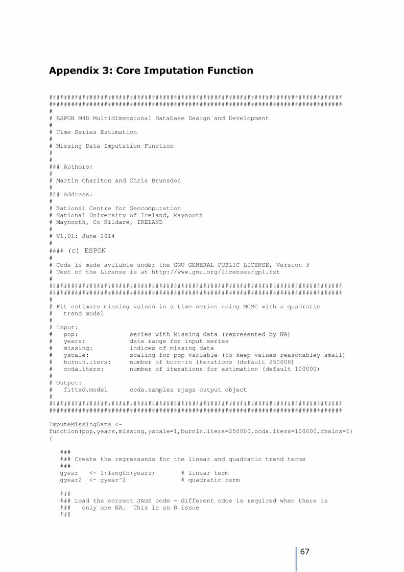
67
Appendix 3: Core Imputation Function
################################################################################
################################################################################
#
# ESPON M4D Multidimensional Database Design and Development
#
# Time Series Estimation
#
# Missing Data Imputation Function
#
#
### Authors:
#
# Martin Charlton and Chris Brunsdon
#
### Address:
#
# National Centre for Geocomputation
# National University of Ireland, Maynooth
# Maynooth, Co Kildare, IRELAND
#
# V1.01: June 2014
#
#### (c) ESPON #
# Code is made avilable under the GNU GENERAL PUBLIC LICENSE, Version 3
# Text of the License is at http://www.gnu.org/licenses/gpl.txt
#
################################################################################
################################################################################
#
# Fit estimate missing values in a time series using MCMC with a quadratic
# trend model
#
# Input:
# pop: series with Missing data (represented by NA)
# years: date range for input series
# missing: indices of missing data
# yscale: scaling for pop variable (to keep values reasonabley small)
# burnin.iters: number of burn-in iterations (default 250000)
# coda.iters: number of iterations for estimation (default 100000)
#
# Output:
# fitted.model coda.samples rjags output object
#
################################################################################
################################################################################
ImputeMissingData <-
function(pop,years,missing,yscale=1,burnin.iters=250000,coda.iters=100000,chains=1)
{
###
### Create the regressands for the linear and quadratic trend terms
###
gyear <- 1:length(years) # linear term
gyear2 <- gyear^2 # quadratic term
###
### Load the correct JAGS code - different cdoe is required when there is
### only one NA. This is an R issue
###
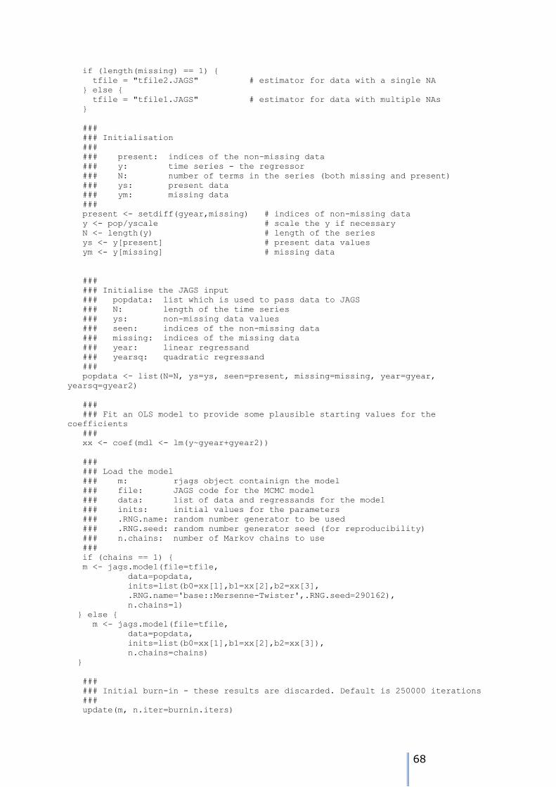
68
if (length(missing) == 1) {
tfile = "tfile2.JAGS" # estimator for data with a single NA
} else {
tfile = "tfile1.JAGS" # estimator for data with multiple NAs
}
###
### Initialisation
###
### present: indices of the non-missing data
### y: time series - the regressor
### N: number of terms in the series (both missing and present)
### ys: present data
### ym: missing data
###
present <- setdiff(gyear,missing) # indices of non-missing data
y <- pop/yscale # scale the y if necessary
N <- length(y) # length of the series
ys <- y[present] # present data values
ym <- y[missing] # missing data
###
### Initialise the JAGS input
### popdata: list which is used to pass data to JAGS
### N: length of the time series
### ys: non-missing data values
### seen: indices of the non-missing data
### missing: indices of the missing data
### year: linear regressand
### yearsq: quadratic regressand
###
popdata <- list(N=N, ys=ys, seen=present, missing=missing, year=gyear,
yearsq=gyear2)
###
### Fit an OLS model to provide some plausible starting values for the
coefficients
###
xx <- coef(mdl <- lm(y~gyear+gyear2))
###
### Load the model
### m: rjags object containign the model
### file: JAGS code for the MCMC model
### data: list of data and regressands for the model
### inits: initial values for the parameters
### .RNG.name: random number generator to be used
### .RNG.seed: random number generator seed (for reproducibility)
### n.chains: number of Markov chains to use
###
if (chains == 1) {
m <- jags.model(file=tfile,
data=popdata,
inits=list(b0=xx[1],b1=xx[2],b2=xx[3],
.RNG.name='base::Mersenne-Twister',.RNG.seed=290162),
n.chains=1)
} else {
m <- jags.model(file=tfile,
data=popdata,
inits=list(b0=xx[1],b1=xx[2],b2=xx[3]),
n.chains=chains)
}
###
### Initial burn-in - these results are discarded. Default is 250000 iterations
###
update(m, n.iter=burnin.iters)

69
###
### Fit the model - output is and mcmc.list object which is returned from the
function
###
coda.samples(m, n.iter=coda.iters, thin=5, variable.names =
c("ym","b0","b1","b2","rho","s2err"))
}
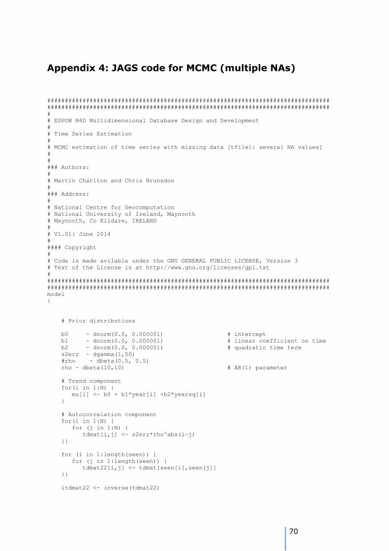
70
Appendix 4: JAGS code for MCMC (multiple NAs)
################################################################################
################################################################################
#
# ESPON M4D Multidimensional Database Design and Development
#
# Time Series Estimation
#
# MCMC estimation of time series with missing data [tfile1: several NA values]
#
#
### Authors:
#
# Martin Charlton and Chris Brunsdon
#
### Address:
#
# National Centre for Geocomputation
# National University of Ireland, Maynooth
# Maynooth, Co Kildare, IRELAND
#
# V1.01: June 2014
#
#### Copyright
#
# Code is made avilable under the GNU GENERAL PUBLIC LICENSE, Version 3
# Text of the License is at http://www.gnu.org/licenses/gpl.txt
#
################################################################################
################################################################################
model
{
# Prior distributions
b0 ~ dnorm(0.0, 0.000001) # intercept
b1 ~ dnorm(0.0, 0.000001) # linear coefficient on time
b2 ~ dnorm(0.0, 0.000001) # quadratic time term
s2err ~ dgamma(1,50)
#rho ~ dbeta(0.5, 0.5)
rho ~ dbeta(10,10) # AR(1) parameter
# Trend component
for(i in 1:N) {
mu[i] <- b0 + b1*year[i] +b2*yearsq[i]
}
# Autocorrelation component
for(i in 1:N) {
for (j in 1:N) {
tdmat[i,j] <- s2err*rho^abs(i-j)
}}
for (i in 1:length(seen)) {
for (j in 1:length(seen)) {
tdmat22[i,j] <- tdmat[seen[i],seen[j]]
}}
itdmat22 <- inverse(tdmat22)
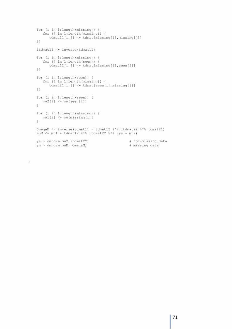
71
for (i in 1:length(missing)) {
for (j in 1:length(missing)) {
tdmat11[i,j] <- tdmat[missing[i],missing[j]]
}}
itdmat11 <- inverse(tdmat11)
for (i in 1:length(missing)) {
for (j in 1:length(seen)) {
tdmat12[i,j] <- tdmat[missing[i],seen[j]]
}}
for (i in 1:length(seen)) {
for (j in 1:length(missing)) {
tdmat21[i,j] <- tdmat[seen[i],missing[j]]
}}
for (i in 1:length(seen)) {
mu2[i] <- mu[seen[i]]
}
for (i in 1:length(missing)) {
mu1[i] <- mu[missing[i]]
}
OmegaM <- inverse(tdmat11 - tdmat12 %*% itdmat22 %*% tdmat21)
muM <- mu1 + tdmat12 %*% itdmat22 %*% (ys - mu2)
ys ~ dmnorm(mu2,itdmat22) # non-missing data
ym ~ dmnorm(muM, OmegaM) # missing data
}

72
Appendix 5: JAGS code for MCMC (single NA)
################################################################################
################################################################################
#
# ESPON M4D Multidimensional Database Design and Development
#
# Time Series Estimation
#
# MCMC estimation of time series with missing data [tfile2: single NA value]
#
#
### Authors:
#
# Martin Charlton and Chris Brunsdon
#
### Address:
#
# National Centre for Geocomputation
# National University of Ireland, Maynooth
# Maynooth, Co Kildare, IRELAND
#
# V1.01: June 2014
#
#### Copyright
#
# Code is made avilable under the GNU GENERAL PUBLIC LICENSE, Version 3
# Text of the License is at http://www.gnu.org/licenses/gpl.txt
#
################################################################################
################################################################################
model
{
# Prior distributions
b0 ~ dnorm(0.0, 0.000001)
b1 ~ dnorm(0.0, 0.000001)
b2 ~ dnorm(0.0, 0.000001)
s2err ~ dgamma(1,50)
#rho ~ dbeta(0.5, 0.5)
rho ~ dbeta(10,10)
# Trend component
for(i in 1:N) {
mu[i] <- b0 + b1*year[i] +b2*yearsq[i]
# mu[i] <- b0 + b1*i
}
# Autocorrelation component
for(i in 1:N) {
for (j in 1:N) {
tdmat[i,j] <- s2err*rho^abs(i-j)
}
}
for (i in 1:length(seen)) {
for (j in 1:length(seen)) {
tdmat22[i,j] <- tdmat[seen[i],seen[j]]
}}
73
itdmat22 <- inverse(tdmat22)
tdmat11 <- tdmat[missing,missing]
itdmat11 <- 1.0/tdmat11
for (j in 1:length(seen)) {
tdmat12[j] <- tdmat[missing,seen[j]]
}
for (i in 1:length(seen)) {
tdmat21[i] <- tdmat[seen[i],missing]
}
for (i in 1:length(seen)) {
mu2[i] <- mu[seen[i]]
}
for (i in 1:length(seen)) {
for (j in 1:length(seen)) {
oprod12[i,j] <- tdmat12[i] * tdmat21[j]
}
}
mu1 <- mu[missing]
OmegaM <- 1.0/(tdmat11 - inprod(tdmat12,itdmat22 %*% tdmat21))
muM <- mu1 + inprod(tdmat12, itdmat22 %*% (ys - mu2))
ys ~ dmnorm(mu2,itdmat22)
ym ~ dnorm(muM, OmegaM)
}
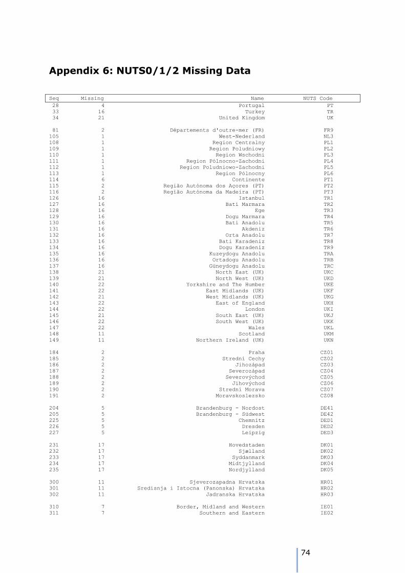
74
Appendix 6: NUTS0/1/2 Missing Data
Seq Missing Name NUTS Code
28 4 Portugal PT
33 16 Turkey TR
34 21 United Kingdom UK
81 2 Départements d'outre-mer (FR) FR9
105 1 West-Nederland NL3
108 1 Region Centralny PL1
109 1 Region Poludniowy PL2
110 1 Region Wschodni PL3
111 1 Region Pólnocno-Zachodni PL4
112 1 Region Poludniowo-Zachodni PL5
113 1 Region Pólnocny PL6
114 6 Continente PT1
115 2 Região Autónoma dos Açores (PT) PT2
116 2 Região Autónoma da Madeira (PT) PT3
126 16 Istanbul TR1
127 16 Bati Marmara TR2
128 16 Ege TR3
129 16 Dogu Marmara TR4
130 16 Bati Anadolu TR5
131 16 Akdeniz TR6
132 16 Orta Anadolu TR7
133 16 Bati Karadeniz TR8
134 16 Dogu Karadeniz TR9
135 16 Kuzeydogu Anadolu TRA
136 16 Ortadogu Anadolu TRB
137 16 Güneydogu Anadolu TRC
138 21 North East (UK) UKC
139 21 North West (UK) UKD
140 22 Yorkshire and The Humber UKE
141 22 East Midlands (UK) UKF
142 21 West Midlands (UK) UKG
143 22 East of England UKH
144 22 London UKI
145 21 South East (UK) UKJ
146 22 South West (UK) UKK
147 22 Wales UKL
148 11 Scotland UKM
149 11 Northern Ireland (UK) UKN
184 2 Praha CZ01
185 2 Strední Cechy CZ02
186 2 Jihozápad CZ03
187 2 Severozápad CZ04
188 2 Severovýchod CZ05
189 2 Jihovýchod CZ06
190 2 Strední Morava CZ07
191 2 Moravskoslezsko CZ08
204 5 Brandenburg - Nordost DE41
205 5 Brandenburg - Südwest DE42
225 5 Chemnitz DED1
226 5 Dresden DED2
227 5 Leipzig DED3
231 17 Hovedstaden DK01
232 17 Sjælland DK02
233 17 Syddanmark DK03
234 17 Midtjylland DK04
235 17 Nordjylland DK05
300 11 Sjeverozapadna Hrvatska HR01
301 11 Sredisnja i Istocna (Panonska) Hrvatska HR02
302 11 Jadranska Hrvatska HR03
310 7 Border, Midland and Western IE01
311 7 Southern and Eastern IE02
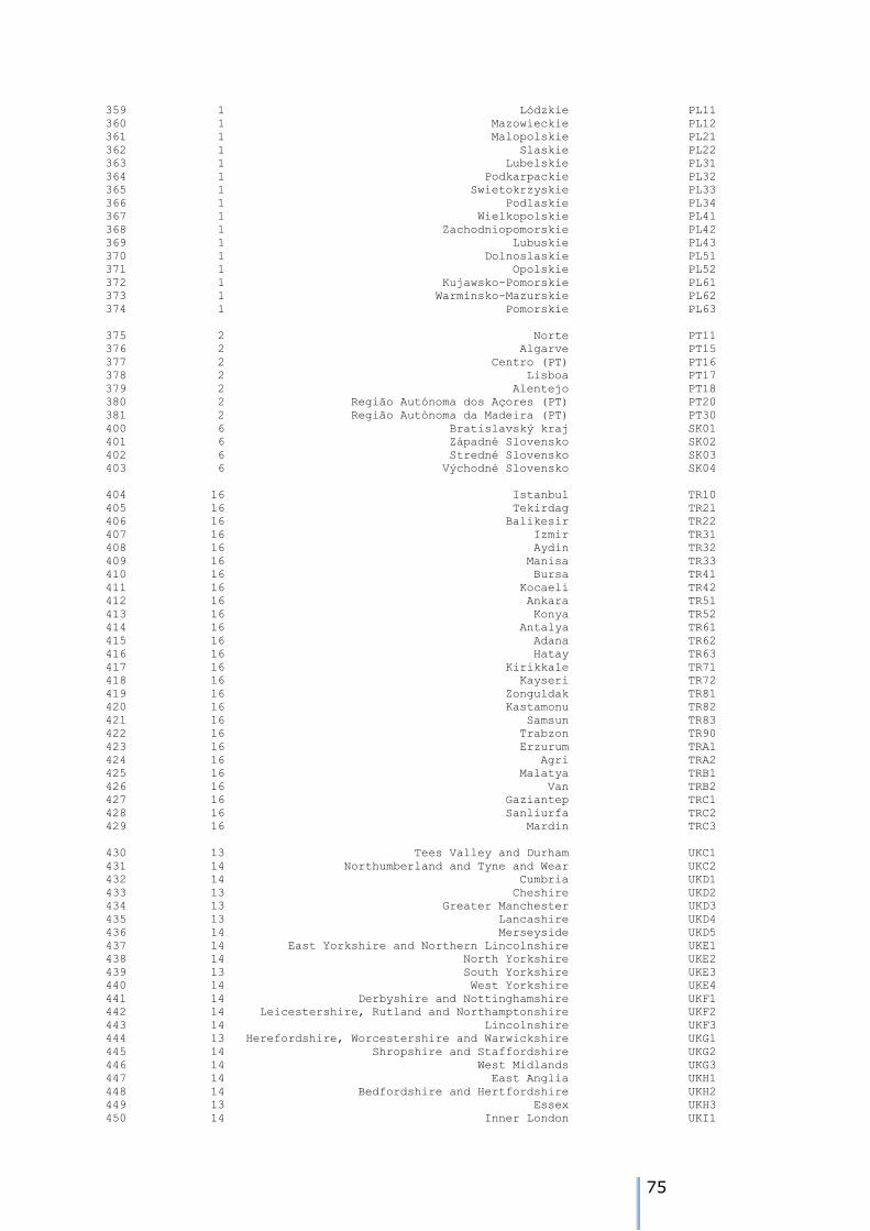
75
359 1 Lódzkie PL11
360 1 Mazowieckie PL12
361 1 Malopolskie PL21
362 1 Slaskie PL22
363 1 Lubelskie PL31
364 1 Podkarpackie PL32
365 1 Swietokrzyskie PL33
366 1 Podlaskie PL34
367 1 Wielkopolskie PL41
368 1 Zachodniopomorskie PL42
369 1 Lubuskie PL43
370 1 Dolnoslaskie PL51
371 1 Opolskie PL52
372 1 Kujawsko-Pomorskie PL61
373 1 Warminsko-Mazurskie PL62
374 1 Pomorskie PL63
375 2 Norte PT11
376 2 Algarve PT15
377 2 Centro (PT) PT16
378 2 Lisboa PT17
379 2 Alentejo PT18
380 2 Região Autónoma dos Açores (PT) PT20
381 2 Região Autónoma da Madeira (PT) PT30
400 6 Bratislavský kraj SK01
401 6 Západné Slovensko SK02
402 6 Stredné Slovensko SK03
403 6 Východné Slovensko SK04
404 16 Istanbul TR10
405 16 Tekirdag TR21
406 16 Balikesir TR22
407 16 Izmir TR31
408 16 Aydin TR32
409 16 Manisa TR33
410 16 Bursa TR41
411 16 Kocaeli TR42
412 16 Ankara TR51
413 16 Konya TR52
414 16 Antalya TR61
415 16 Adana TR62
416 16 Hatay TR63
417 16 Kirikkale TR71
418 16 Kayseri TR72
419 16 Zonguldak TR81
420 16 Kastamonu TR82
421 16 Samsun TR83
422 16 Trabzon TR90
423 16 Erzurum TRA1
424 16 Agri TRA2
425 16 Malatya TRB1
426 16 Van TRB2
427 16 Gaziantep TRC1
428 16 Sanliurfa TRC2
429 16 Mardin TRC3
430 13 Tees Valley and Durham UKC1
431 14 Northumberland and Tyne and Wear UKC2
432 14 Cumbria UKD1
433 13 Cheshire UKD2
434 13 Greater Manchester UKD3
435 13 Lancashire UKD4
436 14 Merseyside UKD5
437 14 East Yorkshire and Northern Lincolnshire UKE1
438 14 North Yorkshire UKE2
439 13 South Yorkshire UKE3
440 14 West Yorkshire UKE4
441 14 Derbyshire and Nottinghamshire UKF1
442 14 Leicestershire, Rutland and Northamptonshire UKF2
443 14 Lincolnshire UKF3
444 13 Herefordshire, Worcestershire and Warwickshire UKG1
445 14 Shropshire and Staffordshire UKG2
446 14 West Midlands UKG3
447 14 East Anglia UKH1
448 14 Bedfordshire and Hertfordshire UKH2
449 13 Essex UKH3
450 14 Inner London UKI1

76
451 14 Outer London UKI2
452 13 Berkshire, Buckinghamshire and Oxfordshire UKJ1
453 14 Surrey, East and West Sussex UKJ2
454 14 Hampshire and Isle of Wight UKJ3
455 13 Kent UKJ4
456 13 Gloucestershire, Wiltshire and Bristol/Bath area UKK1
457 13 Dorset and Somerset UKK2
458 13 Cornwall and Isles of Scilly UKK3
459 13 Devon UKK4
460 13 West Wales and The Valleys UKL1
461 13 East Wales UKL2
462 22 Eastern Scotland UKM2
463 21 South Western Scotland UKM3
464 21 North Eastern Scotland UKM5
465 21 Highlands and Islands UKM6
466 11 Northern Ireland (UK) UKN0

77
Appendix 7: Missing Data HeatMaps
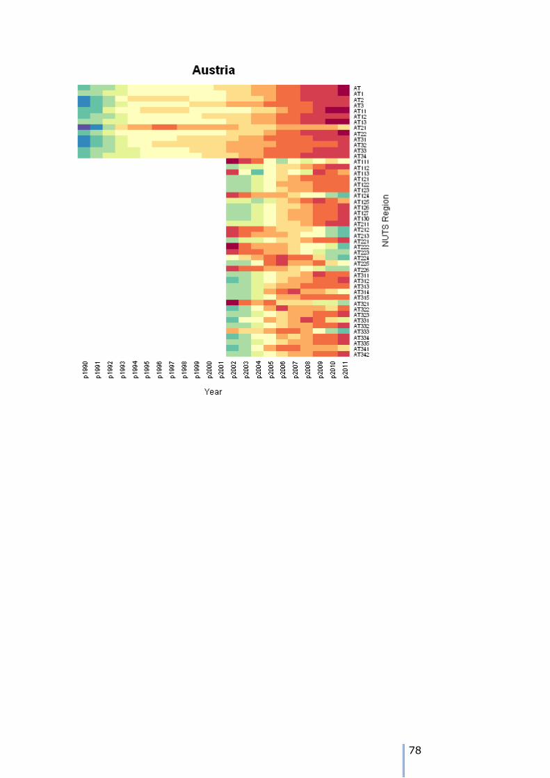
78
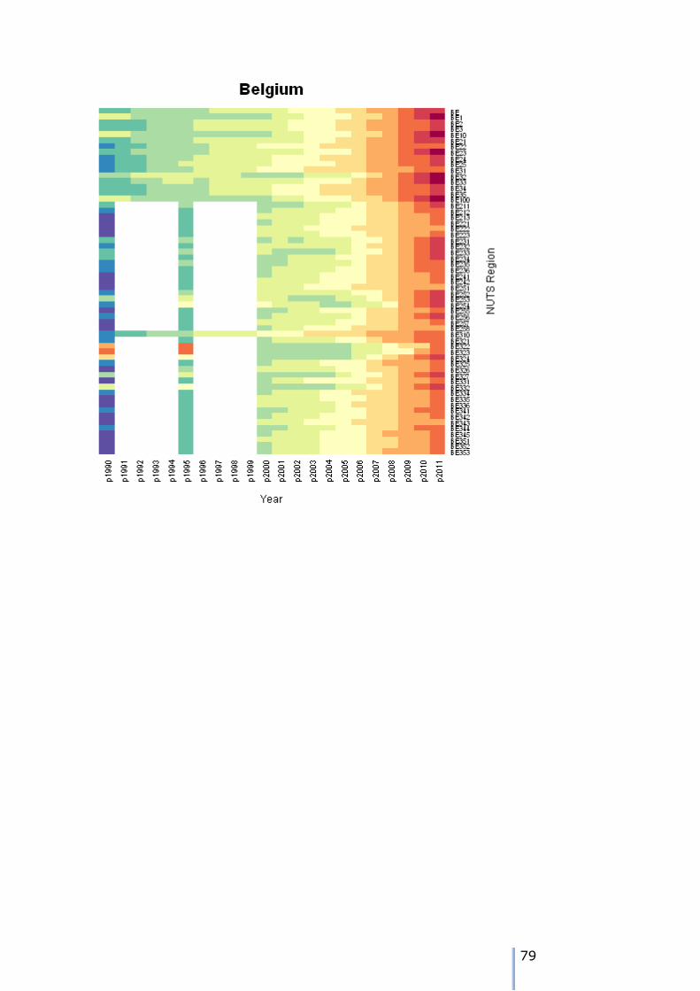
79
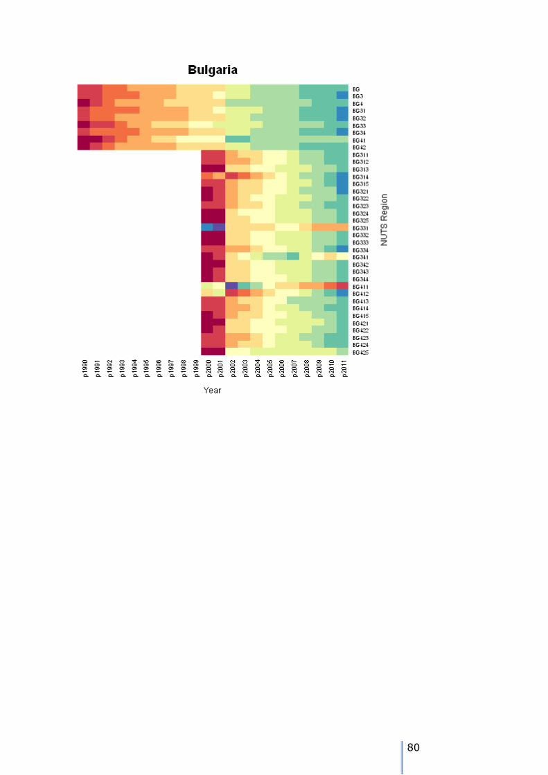
80
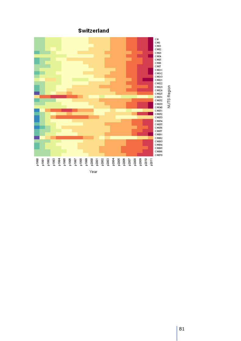
81

82
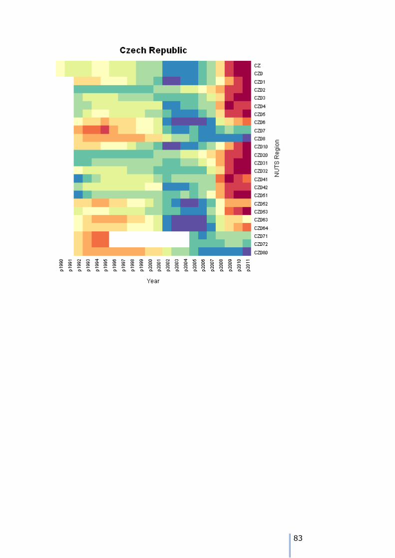
83
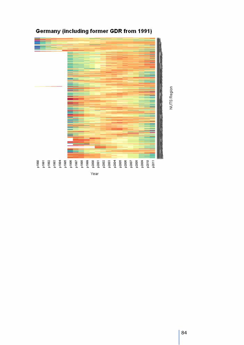
84
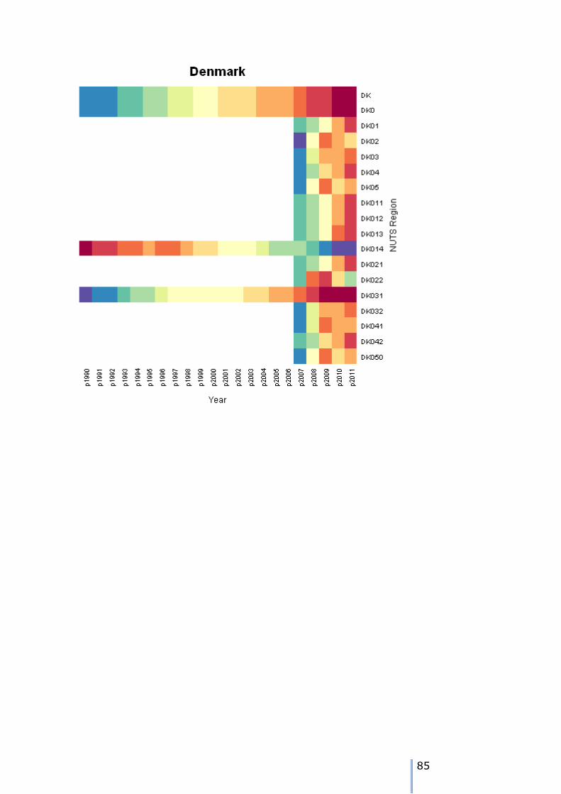
85
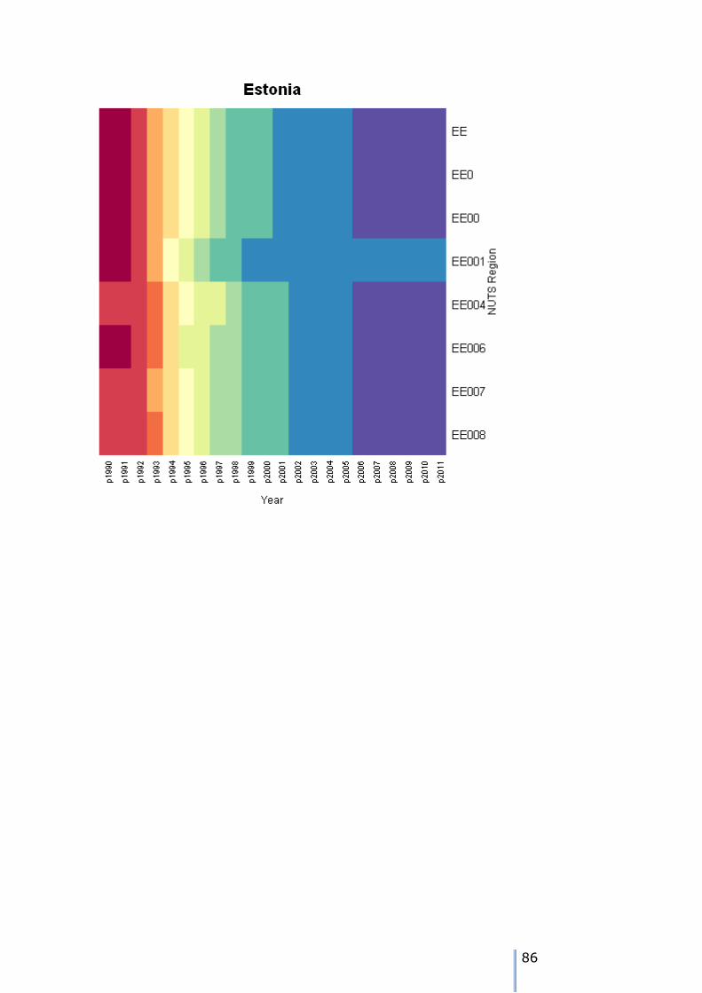
86
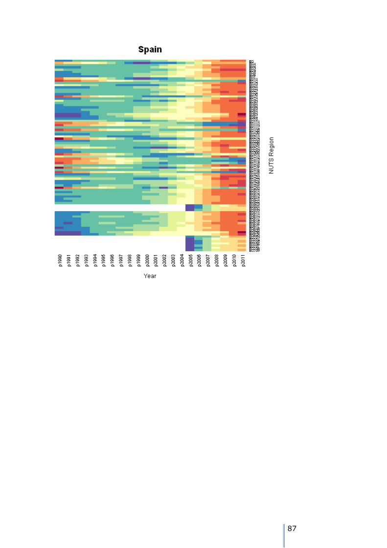
87
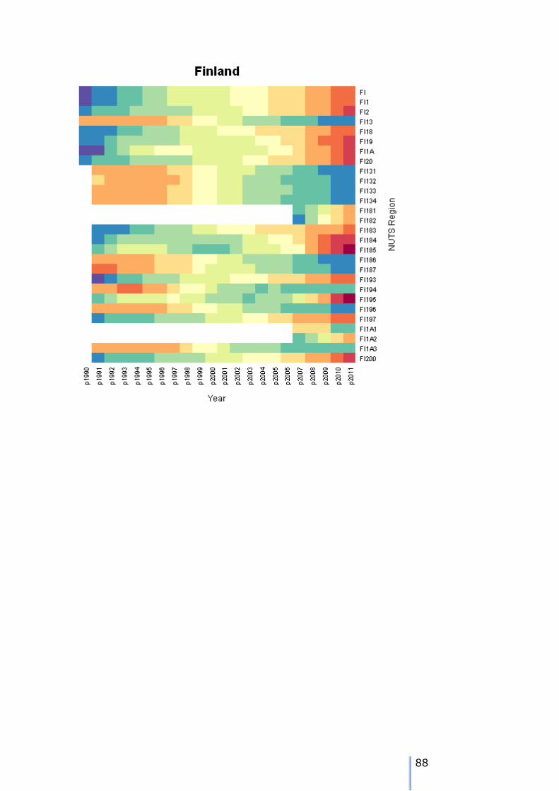
88
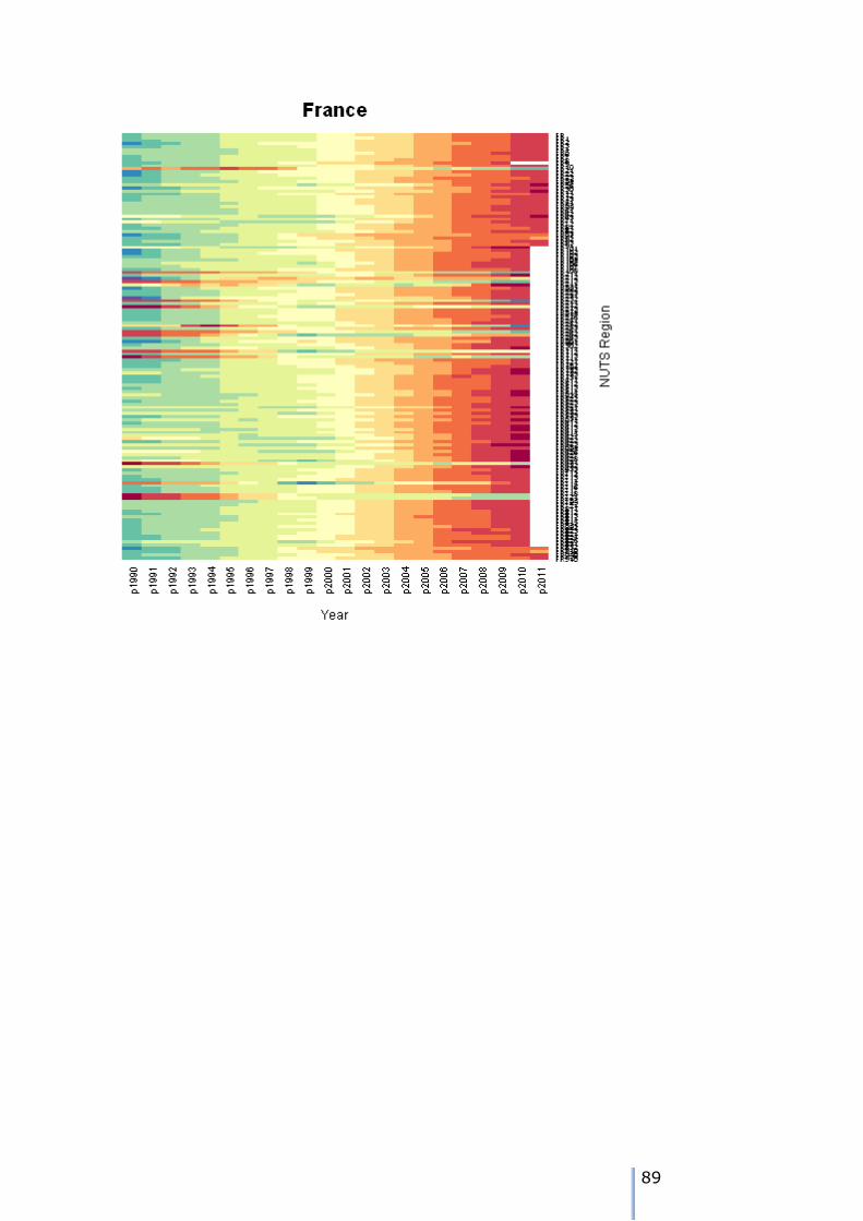
89
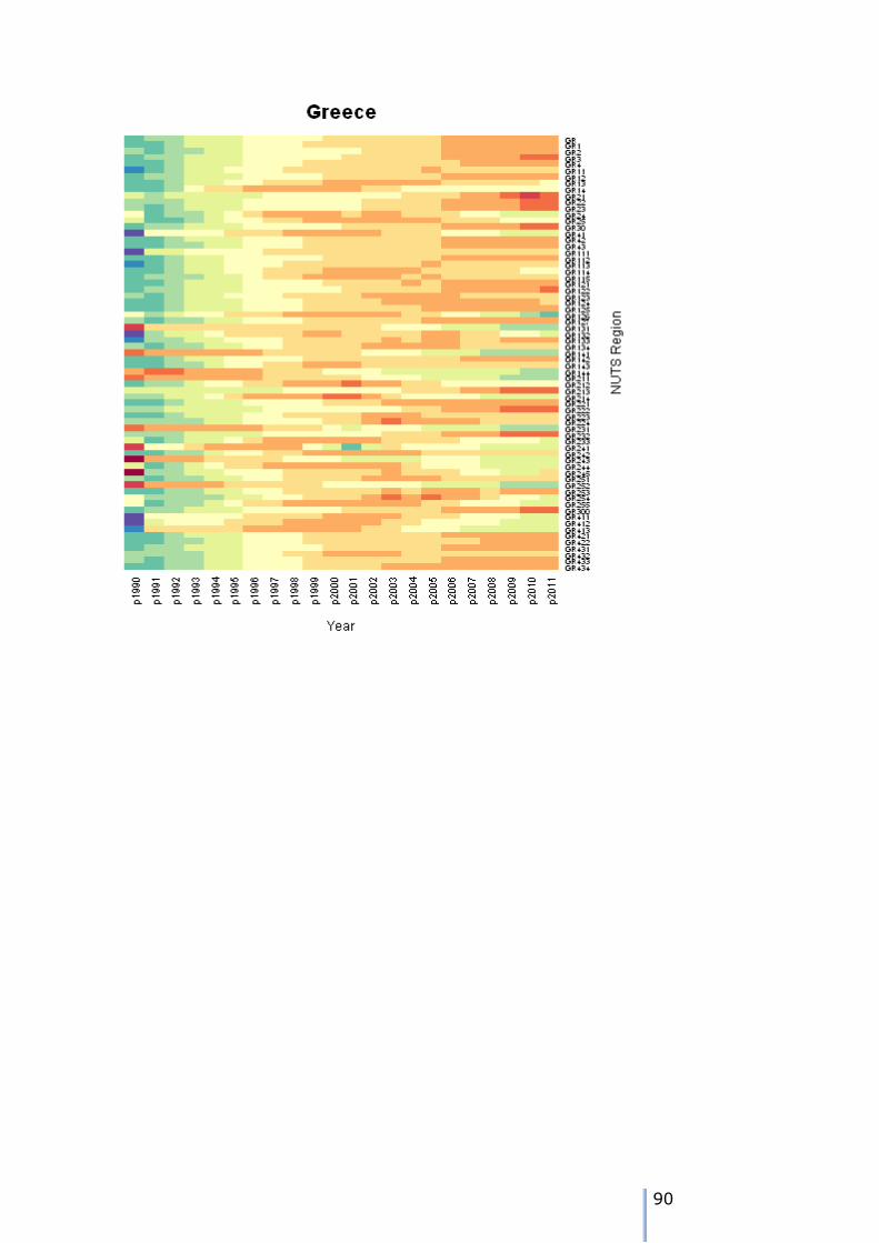
90
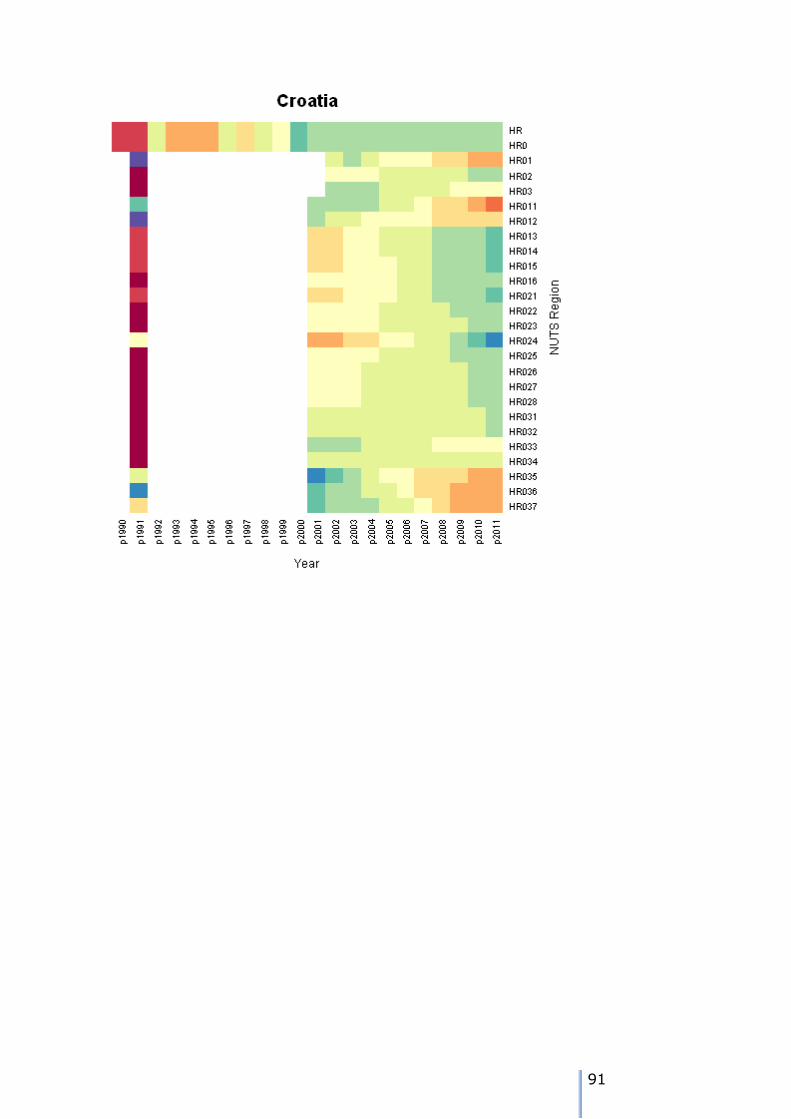
91
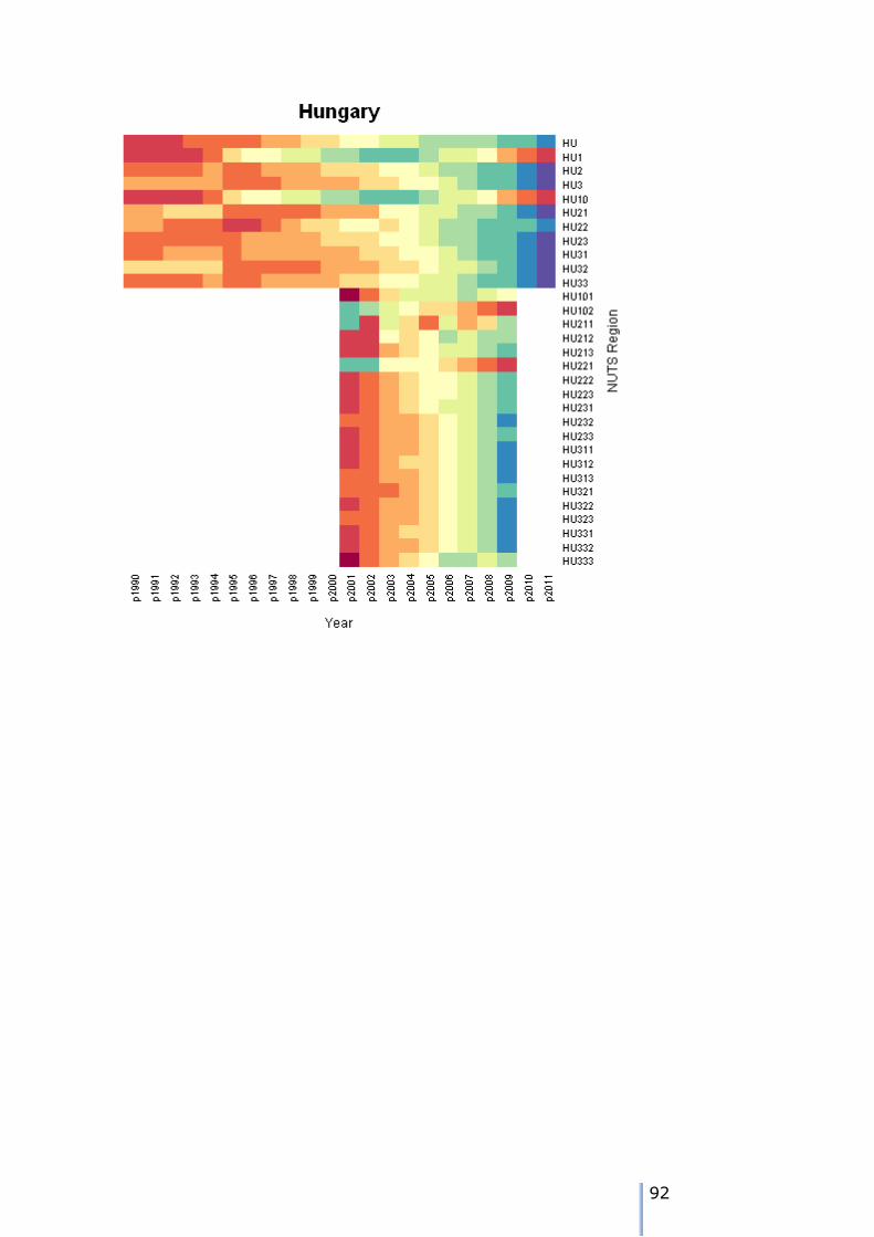
92
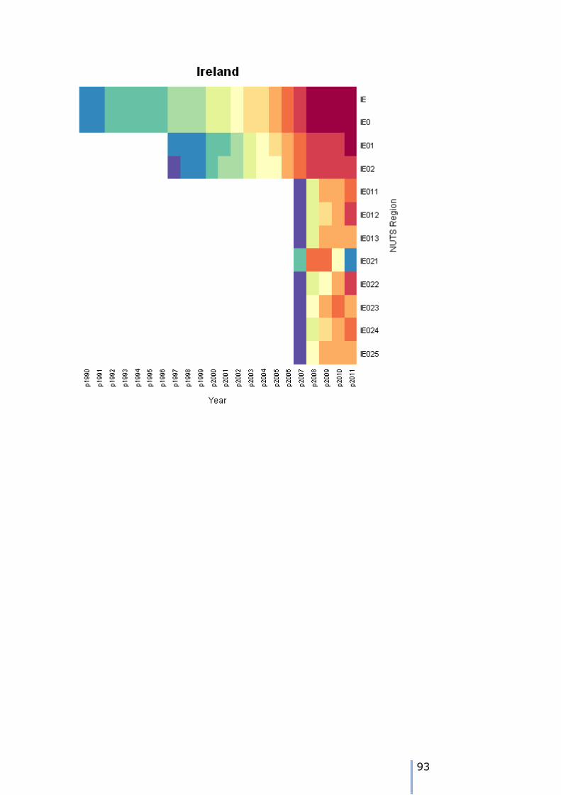
93
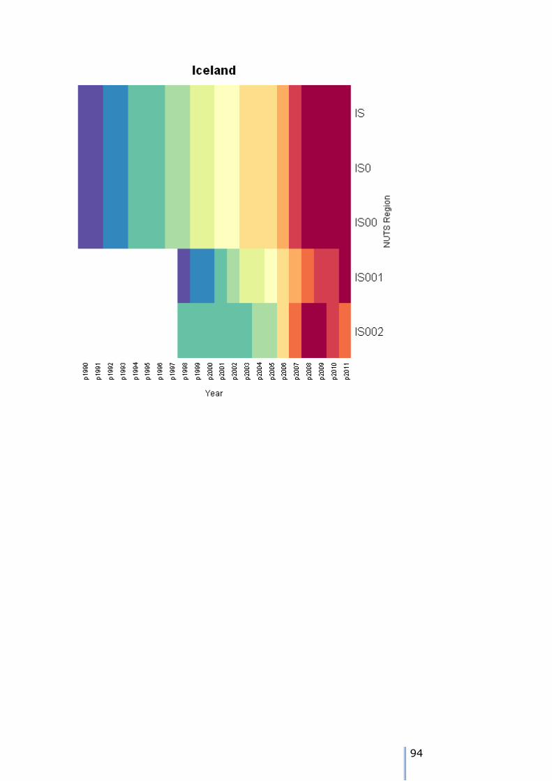
94
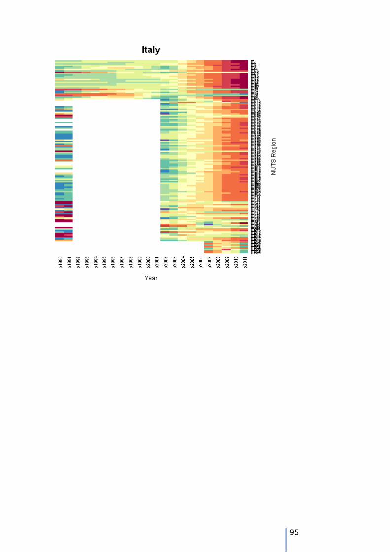
95
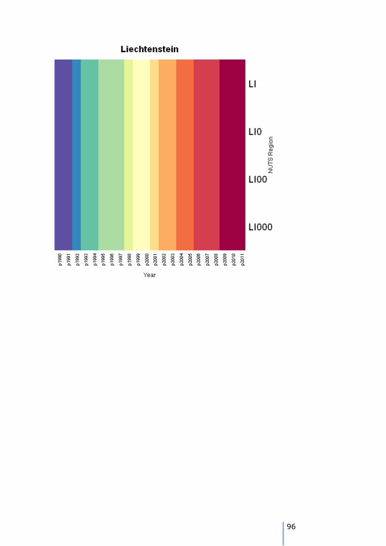
96
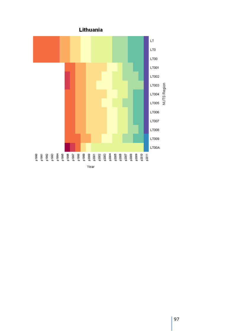
97

98
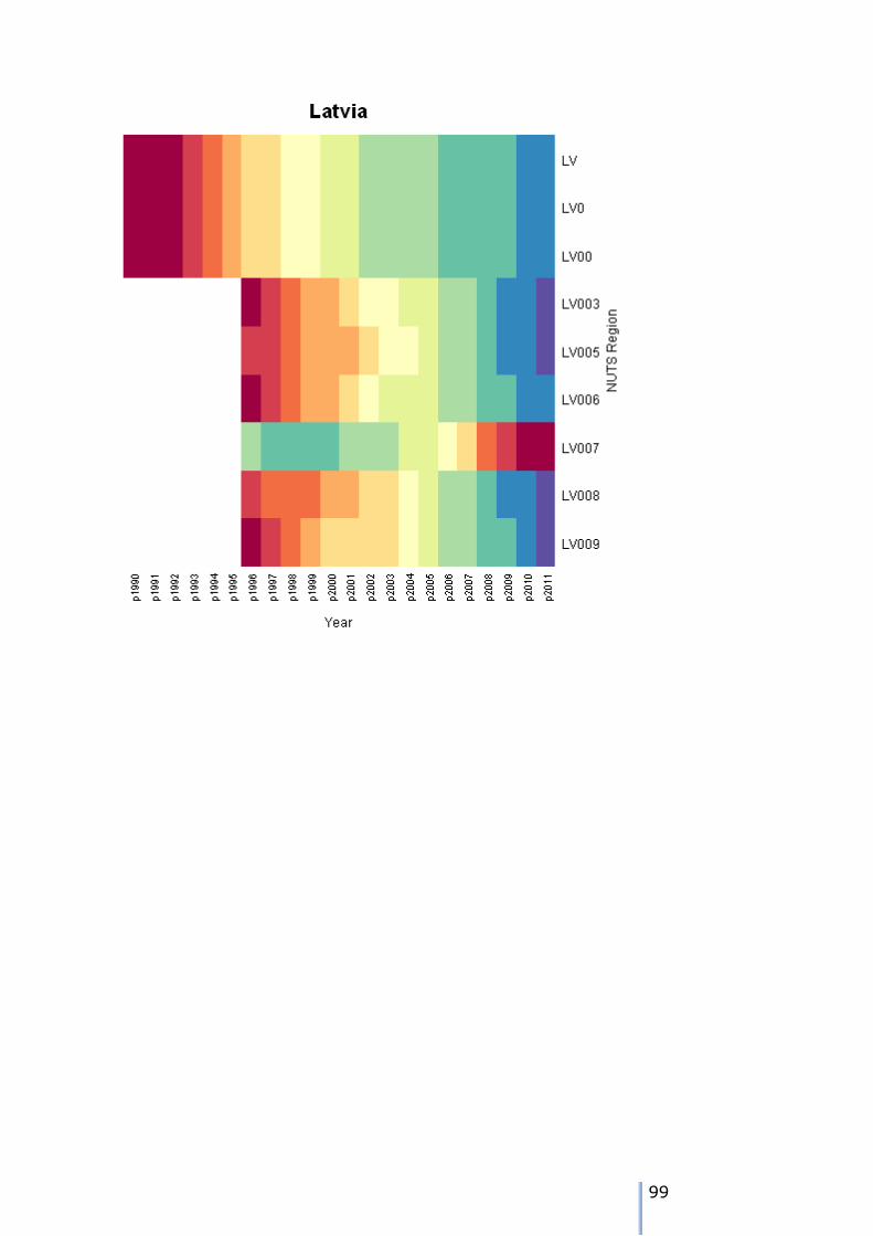
99
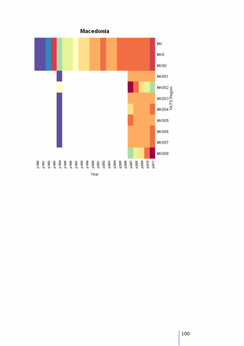
100
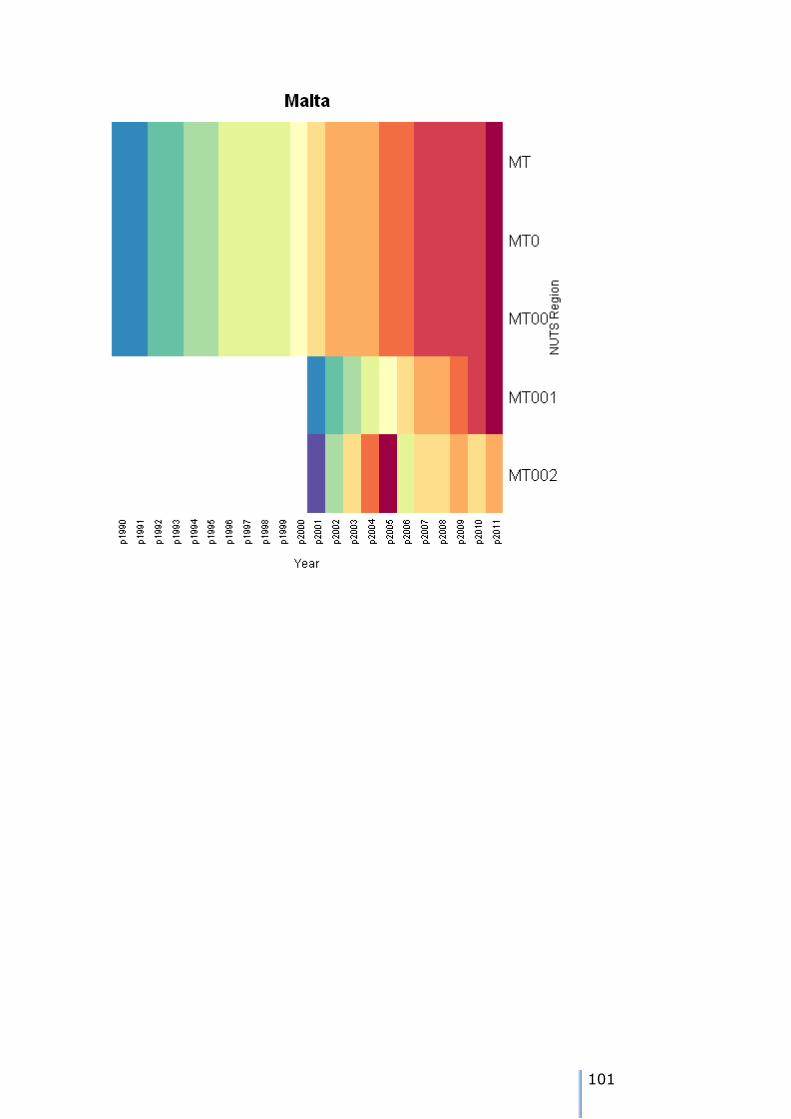
101
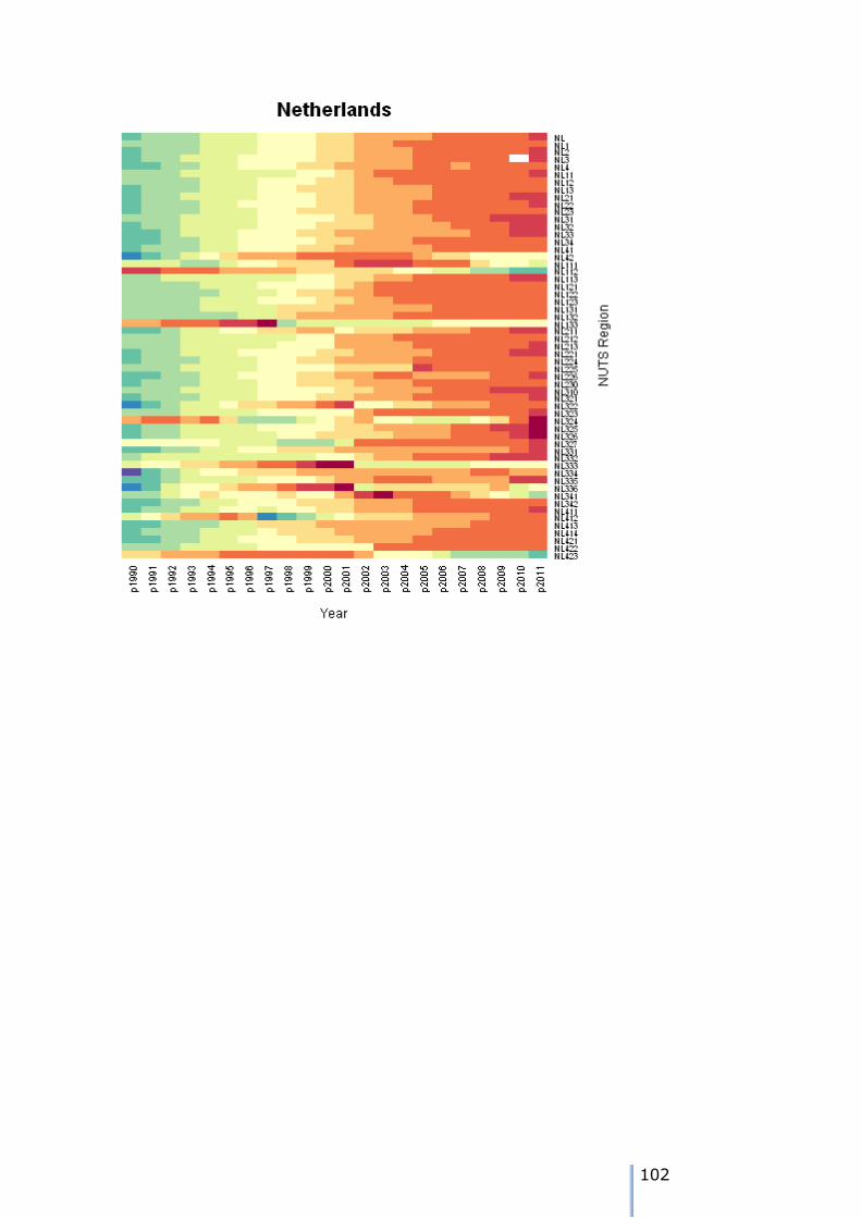
102
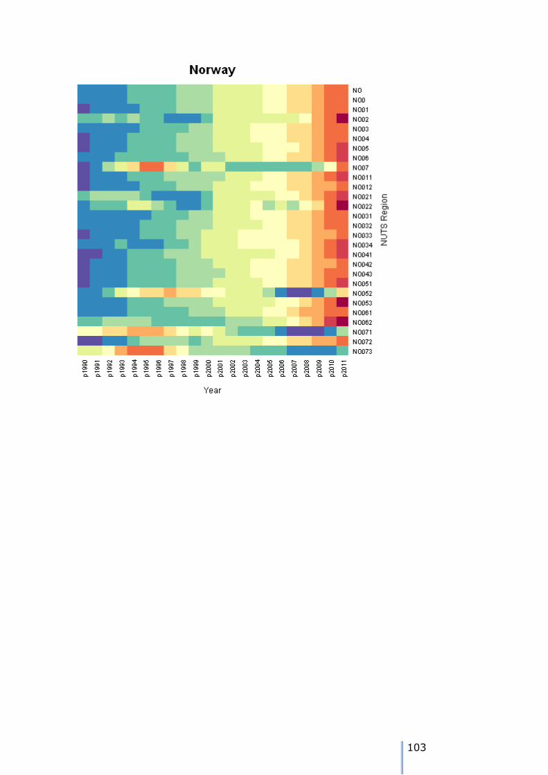
103
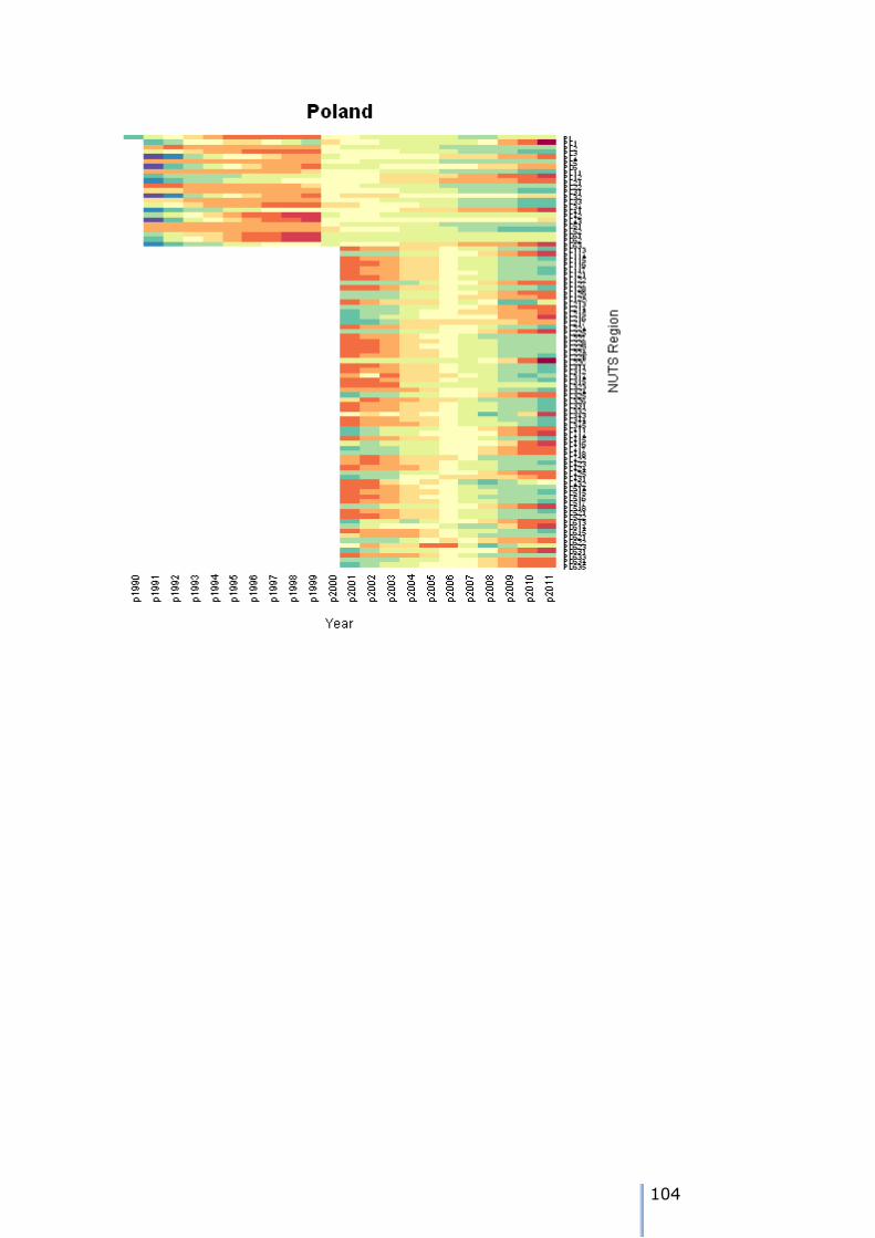
104
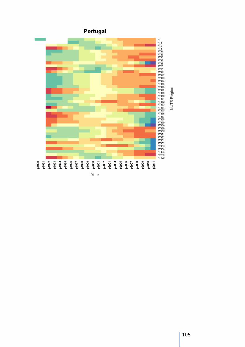
105
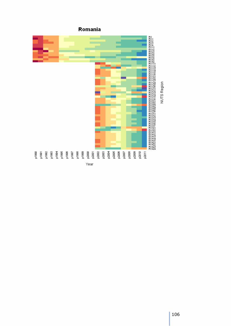
106
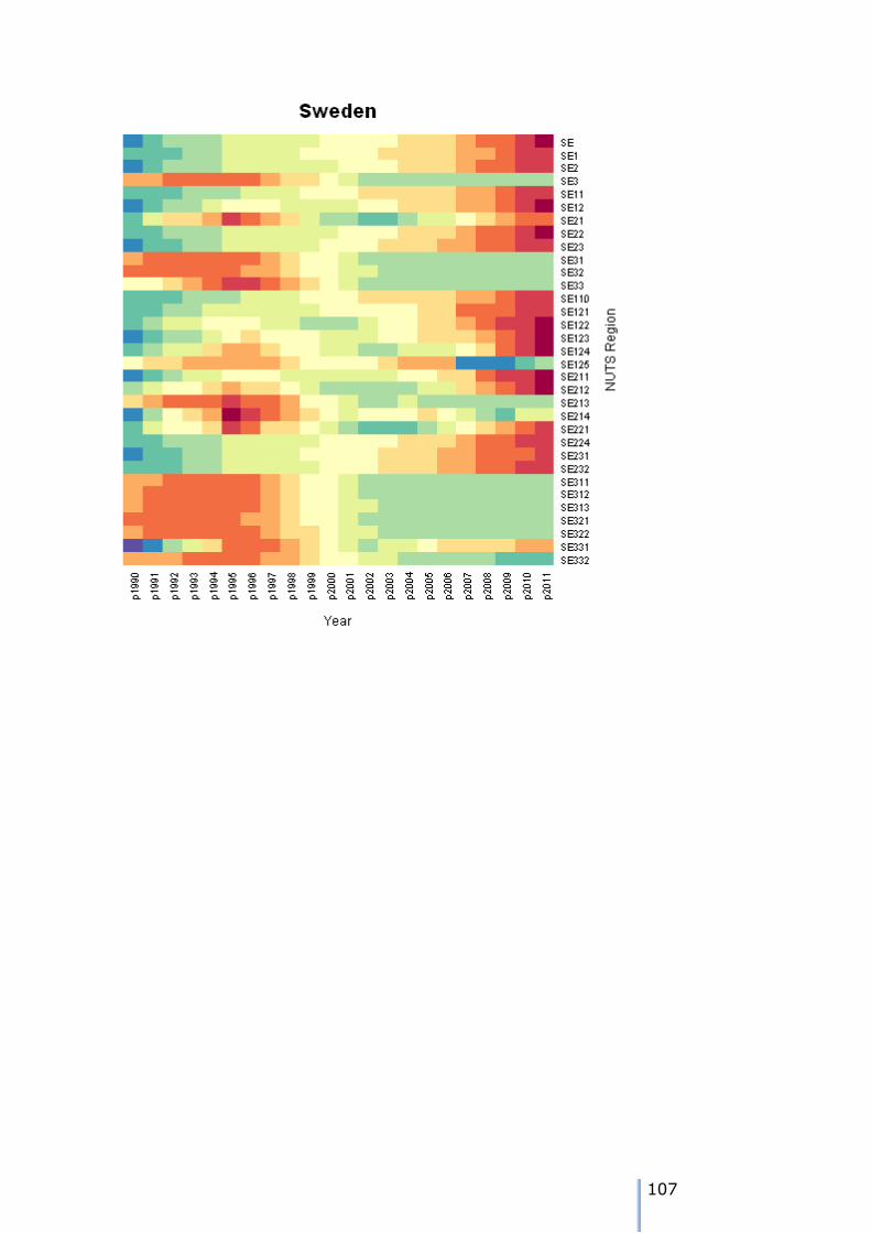
107
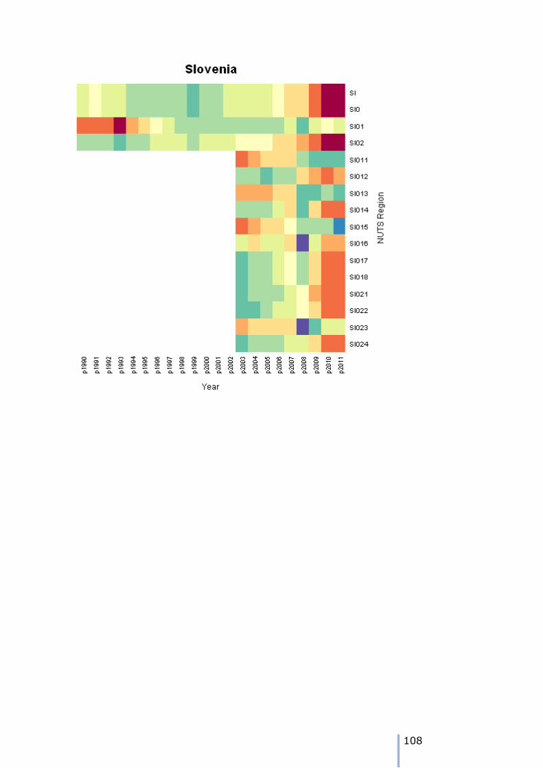
108
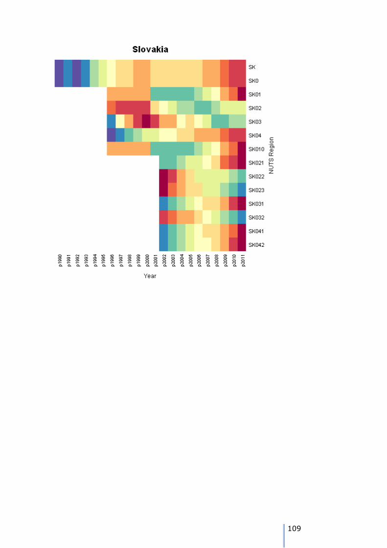
109
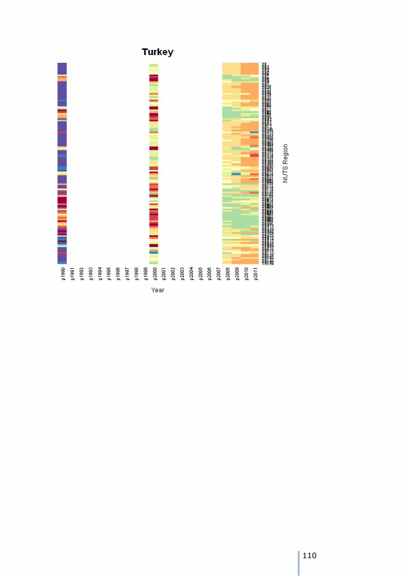
110
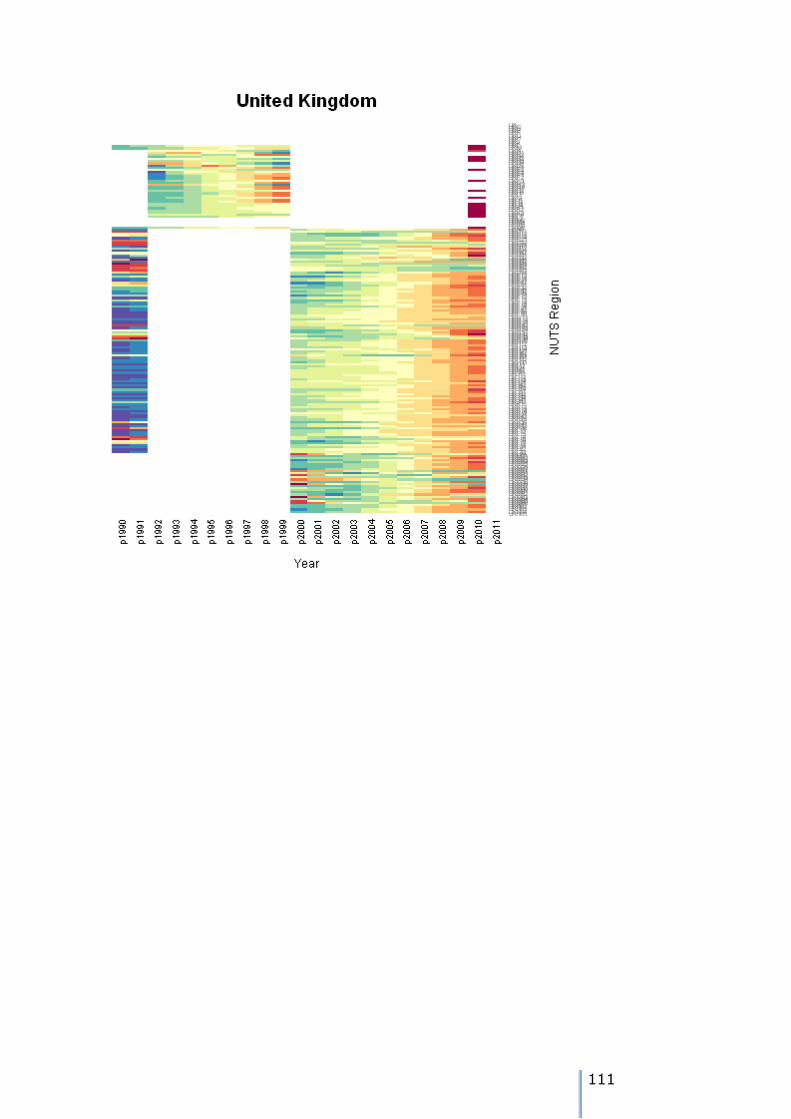
111
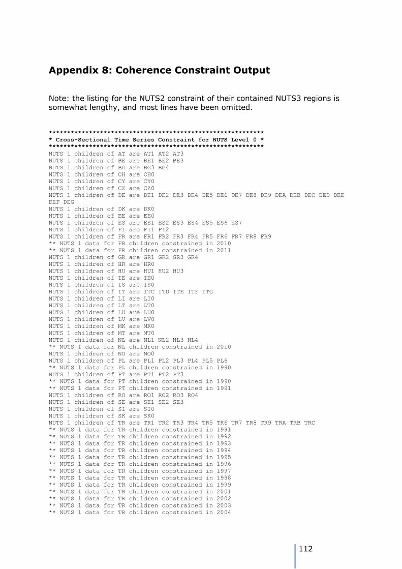
112
Appendix 8: Coherence Constraint Output
Note: the listing for the NUTS2 constraint of their contained NUTS3 regions is somewhat lengthy, and most lines have been omitted.
***********************************************************
* Cross-Sectional Time Series Constraint for NUTS Level 0 *
***********************************************************
NUTS 1 children of AT are AT1 AT2 AT3
NUTS 1 children of BE are BE1 BE2 BE3
NUTS 1 children of BG are BG3 BG4
NUTS 1 children of CH are CH0
NUTS 1 children of CY are CY0
NUTS 1 children of CZ are CZ0
NUTS 1 children of DE are DE1 DE2 DE3 DE4 DE5 DE6 DE7 DE8 DE9 DEA DEB DEC DED DEE
DEF DEG
NUTS 1 children of DK are DK0
NUTS 1 children of EE are EE0
NUTS 1 children of ES are ES1 ES2 ES3 ES4 ES5 ES6 ES7
NUTS 1 children of FI are FI1 FI2
NUTS 1 children of FR are FR1 FR2 FR3 FR4 FR5 FR6 FR7 FR8 FR9
** NUTS 1 data for FR children constrained in 2010
** NUTS 1 data for FR children constrained in 2011
NUTS 1 children of GR are GR1 GR2 GR3 GR4
NUTS 1 children of HR are HR0
NUTS 1 children of HU are HU1 HU2 HU3
NUTS 1 children of IE are IE0
NUTS 1 children of IS are IS0
NUTS 1 children of IT are ITC ITD ITE ITF ITG
NUTS 1 children of LI are LI0
NUTS 1 children of LT are LT0
NUTS 1 children of LU are LU0
NUTS 1 children of LV are LV0
NUTS 1 children of MK are MK0
NUTS 1 children of MT are MT0
NUTS 1 children of NL are NL1 NL2 NL3 NL4
** NUTS 1 data for NL children constrained in 2010
NUTS 1 children of NO are NO0
NUTS 1 children of PL are PL1 PL2 PL3 PL4 PL5 PL6
** NUTS 1 data for PL children constrained in 1990
NUTS 1 children of PT are PT1 PT2 PT3
** NUTS 1 data for PT children constrained in 1990
** NUTS 1 data for PT children constrained in 1991
NUTS 1 children of RO are RO1 RO2 RO3 RO4
NUTS 1 children of SE are SE1 SE2 SE3
NUTS 1 children of SI are SI0
NUTS 1 children of SK are SK0
NUTS 1 children of TR are TR1 TR2 TR3 TR4 TR5 TR6 TR7 TR8 TR9 TRA TRB TRC
** NUTS 1 data for TR children constrained in 1991
** NUTS 1 data for TR children constrained in 1992
** NUTS 1 data for TR children constrained in 1993
** NUTS 1 data for TR children constrained in 1994
** NUTS 1 data for TR children constrained in 1995
** NUTS 1 data for TR children constrained in 1996
** NUTS 1 data for TR children constrained in 1997
** NUTS 1 data for TR children constrained in 1998
** NUTS 1 data for TR children constrained in 1999
** NUTS 1 data for TR children constrained in 2001
** NUTS 1 data for TR children constrained in 2002
** NUTS 1 data for TR children constrained in 2003
** NUTS 1 data for TR children constrained in 2004
113
** NUTS 1 data for TR children constrained in 2005
** NUTS 1 data for TR children constrained in 2006
** NUTS 1 data for TR children constrained in 2007
NUTS 1 children of UK are UKC UKD UKE UKF UKG UKH UKI UKJ UKK UKL UKM UKN
** NUTS 1 data for UK children constrained in 2011
***********************************************************
* Cross-Sectional Time Series Constraint for NUTS Level 1 *
***********************************************************
NUTS 2 children of AT1 are AT11 AT12 AT13
NUTS 2 children of AT2 are AT21 AT22
NUTS 2 children of AT3 are AT31 AT32 AT33 AT34
NUTS 2 children of BE1 are BE10
NUTS 2 children of BE2 are BE21 BE22 BE23 BE24 BE25
NUTS 2 children of BE3 are BE31 BE32 BE33 BE34 BE35
NUTS 2 children of BG3 are BG31 BG32 BG33 BG34
NUTS 2 children of BG4 are BG41 BG42
NUTS 2 children of CH0 are CH01 CH02 CH03 CH04 CH05 CH06 CH07
NUTS 2 children of CY0 are CY00
NUTS 2 children of CZ0 are CZ01 CZ02 CZ03 CZ04 CZ05 CZ06 CZ07 CZ08
** NUTS 2 data for CZ0 children constrained in 1990
** NUTS 2 data for CZ0 children constrained in 1991
NUTS 2 children of DE1 are DE11 DE12 DE13 DE14
NUTS 2 children of DE2 are DE21 DE22 DE23 DE24 DE25 DE26 DE27
NUTS 2 children of DE3 are DE30
NUTS 2 children of DE4 are DE41 DE42
** NUTS 2 data for DE4 children constrained in 1990
** NUTS 2 data for DE4 children constrained in 1991
** NUTS 2 data for DE4 children constrained in 1992
** NUTS 2 data for DE4 children constrained in 1993
** NUTS 2 data for DE4 children constrained in 1994
NUTS 2 children of DE5 are DE50
NUTS 2 children of DE6 are DE60
NUTS 2 children of DE7 are DE71 DE72 DE73
NUTS 2 children of DE8 are DE80
NUTS 2 children of DE9 are DE91 DE92 DE93 DE94
NUTS 2 children of DEA are DEA1 DEA2 DEA3 DEA4 DEA5
NUTS 2 children of DEB are DEB1 DEB2 DEB3
NUTS 2 children of DEC are DEC0
NUTS 2 children of DED are DED1 DED2 DED3
** NUTS 2 data for DED children constrained in 1990
** NUTS 2 data for DED children constrained in 1991
** NUTS 2 data for DED children constrained in 1992
** NUTS 2 data for DED children constrained in 1993
** NUTS 2 data for DED children constrained in 1994
NUTS 2 children of DEE are DEE0
NUTS 2 children of DEF are DEF0
NUTS 2 children of DEG are DEG0
NUTS 2 children of DK0 are DK01 DK02 DK03 DK04 DK05
** NUTS 2 data for DK0 children constrained in 1990
** NUTS 2 data for DK0 children constrained in 1991
** NUTS 2 data for DK0 children constrained in 1992
** NUTS 2 data for DK0 children constrained in 1993
** NUTS 2 data for DK0 children constrained in 1994
** NUTS 2 data for DK0 children constrained in 1995
** NUTS 2 data for DK0 children constrained in 1996
** NUTS 2 data for DK0 children constrained in 1997
** NUTS 2 data for DK0 children constrained in 1998
** NUTS 2 data for DK0 children constrained in 1999
** NUTS 2 data for DK0 children constrained in 2000
** NUTS 2 data for DK0 children constrained in 2001
** NUTS 2 data for DK0 children constrained in 2002
** NUTS 2 data for DK0 children constrained in 2003
** NUTS 2 data for DK0 children constrained in 2004
** NUTS 2 data for DK0 children constrained in 2005
** NUTS 2 data for DK0 children constrained in 2006
NUTS 2 children of EE0 are EE00

114
NUTS 2 children of ES1 are ES11 ES12 ES13
NUTS 2 children of ES2 are ES21 ES22 ES23 ES24
NUTS 2 children of ES3 are ES30
NUTS 2 children of ES4 are ES41 ES42 ES43
NUTS 2 children of ES5 are ES51 ES52 ES53
NUTS 2 children of ES6 are ES61 ES62 ES63 ES64
NUTS 2 children of ES7 are ES70
NUTS 2 children of FI1 are FI13 FI18 FI19 FI1A
NUTS 2 children of FI2 are FI20
NUTS 2 children of FR1 are FR10
NUTS 2 children of FR2 are FR21 FR22 FR23 FR24 FR25 FR26
NUTS 2 children of FR3 are FR30
NUTS 2 children of FR4 are FR41 FR42 FR43
NUTS 2 children of FR5 are FR51 FR52 FR53
NUTS 2 children of FR6 are FR61 FR62 FR63
NUTS 2 children of FR7 are FR71 FR72
NUTS 2 children of FR8 are FR81 FR82 FR83
NUTS 2 children of FR9 are FR91 FR92 FR93 FR94
NUTS 2 children of GR1 are GR11 GR12 GR13 GR14
NUTS 2 children of GR2 are GR21 GR22 GR23 GR24 GR25
NUTS 2 children of GR3 are GR30
NUTS 2 children of GR4 are GR41 GR42 GR43
NUTS 2 children of HR0 are HR01 HR02 HR03
** NUTS 2 data for HR0 children constrained in 1990
** NUTS 2 data for HR0 children constrained in 1992
** NUTS 2 data for HR0 children constrained in 1993
** NUTS 2 data for HR0 children constrained in 1994
** NUTS 2 data for HR0 children constrained in 1995
** NUTS 2 data for HR0 children constrained in 1996
** NUTS 2 data for HR0 children constrained in 1997
** NUTS 2 data for HR0 children constrained in 1998
** NUTS 2 data for HR0 children constrained in 1999
** NUTS 2 data for HR0 children constrained in 2000
** NUTS 2 data for HR0 children constrained in 2001
NUTS 2 children of HU1 are HU10
NUTS 2 children of HU2 are HU21 HU22 HU23
NUTS 2 children of HU3 are HU31 HU32 HU33
NUTS 2 children of IE0 are IE01 IE02
** NUTS 2 data for IE0 children constrained in 1990
** NUTS 2 data for IE0 children constrained in 1991
** NUTS 2 data for IE0 children constrained in 1992
** NUTS 2 data for IE0 children constrained in 1993
** NUTS 2 data for IE0 children constrained in 1994
** NUTS 2 data for IE0 children constrained in 1995
** NUTS 2 data for IE0 children constrained in 1996
NUTS 2 children of IS0 are IS00
NUTS 2 children of ITC are ITC1 ITC2 ITC3 ITC4
NUTS 2 children of ITD are ITD1 ITD2 ITD3 ITD4 ITD5
NUTS 2 children of ITE are ITE1 ITE2 ITE3 ITE4
NUTS 2 children of ITF are ITF1 ITF2 ITF3 ITF4 ITF5 ITF6
NUTS 2 children of ITG are ITG1 ITG2
NUTS 2 children of LI0 are LI00
NUTS 2 children of LT0 are LT00
NUTS 2 children of LU0 are LU00
NUTS 2 children of LV0 are LV00
NUTS 2 children of MK0 are MK00
NUTS 2 children of MT0 are MT00
NUTS 2 children of NL1 are NL11 NL12 NL13
NUTS 2 children of NL2 are NL21 NL22 NL23
NUTS 2 children of NL3 are NL31 NL32 NL33 NL34
NUTS 2 children of NL4 are NL41 NL42
NUTS 2 children of NO0 are NO01 NO02 NO03 NO04 NO05 NO06 NO07
NUTS 2 children of PL1 are PL11 PL12
** NUTS 2 data for PL1 children constrained in 1990
NUTS 2 children of PL2 are PL21 PL22
** NUTS 2 data for PL2 children constrained in 1990
NUTS 2 children of PL3 are PL31 PL32 PL33 PL34
** NUTS 2 data for PL3 children constrained in 1990
115
NUTS 2 children of PL4 are PL41 PL42 PL43
** NUTS 2 data for PL4 children constrained in 1990
NUTS 2 children of PL5 are PL51 PL52
** NUTS 2 data for PL5 children constrained in 1990
NUTS 2 children of PL6 are PL61 PL62 PL63
** NUTS 2 data for PL6 children constrained in 1990
NUTS 2 children of PT1 are PT11 PT15 PT16 PT17 PT18
** NUTS 2 data for PT1 children constrained in 1990
** NUTS 2 data for PT1 children constrained in 1991
NUTS 2 children of PT2 are PT20
** NUTS 2 data for PT2 children constrained in 1990
** NUTS 2 data for PT2 children constrained in 1991
NUTS 2 children of PT3 are PT30
** NUTS 2 data for PT3 children constrained in 1990
** NUTS 2 data for PT3 children constrained in 1991
NUTS 2 children of RO1 are RO11 RO12
NUTS 2 children of RO2 are RO21 RO22
NUTS 2 children of RO3 are RO31 RO32
NUTS 2 children of RO4 are RO41 RO42
NUTS 2 children of SE1 are SE11 SE12
NUTS 2 children of SE2 are SE21 SE22 SE23
NUTS 2 children of SE3 are SE31 SE32 SE33
NUTS 2 children of SI0 are SI01 SI02
NUTS 2 children of SK0 are SK01 SK02 SK03 SK04
** NUTS 2 data for SK0 children constrained in 1990
** NUTS 2 data for SK0 children constrained in 1991
** NUTS 2 data for SK0 children constrained in 1992
** NUTS 2 data for SK0 children constrained in 1993
** NUTS 2 data for SK0 children constrained in 1994
** NUTS 2 data for SK0 children constrained in 1995
NUTS 2 children of TR1 are TR10
** NUTS 2 data for TR1 children constrained in 1991
** NUTS 2 data for TR1 children constrained in 1992
** NUTS 2 data for TR1 children constrained in 1993
** NUTS 2 data for TR1 children constrained in 1994
** NUTS 2 data for TR1 children constrained in 1995
** NUTS 2 data for TR1 children constrained in 1996
** NUTS 2 data for TR1 children constrained in 1997
** NUTS 2 data for TR1 children constrained in 1998
** NUTS 2 data for TR1 children constrained in 1999
** NUTS 2 data for TR1 children constrained in 2001
** NUTS 2 data for TR1 children constrained in 2002
** NUTS 2 data for TR1 children constrained in 2003
** NUTS 2 data for TR1 children constrained in 2004
** NUTS 2 data for TR1 children constrained in 2005
** NUTS 2 data for TR1 children constrained in 2006
** NUTS 2 data for TR1 children constrained in 2007
NUTS 2 children of TR2 are TR21 TR22
** NUTS 2 data for TR2 children constrained in 1991
** NUTS 2 data for TR2 children constrained in 1992
** NUTS 2 data for TR2 children constrained in 1993
** NUTS 2 data for TR2 children constrained in 1994
** NUTS 2 data for TR2 children constrained in 1995
** NUTS 2 data for TR2 children constrained in 1996
** NUTS 2 data for TR2 children constrained in 1997
** NUTS 2 data for TR2 children constrained in 1998
** NUTS 2 data for TR2 children constrained in 1999
** NUTS 2 data for TR2 children constrained in 2001
** NUTS 2 data for TR2 children constrained in 2002
** NUTS 2 data for TR2 children constrained in 2003
** NUTS 2 data for TR2 children constrained in 2004
** NUTS 2 data for TR2 children constrained in 2005
** NUTS 2 data for TR2 children constrained in 2006
** NUTS 2 data for TR2 children constrained in 2007
NUTS 2 children of TR3 are TR31 TR32 TR33
** NUTS 2 data for TR3 children constrained in 1991
** NUTS 2 data for TR3 children constrained in 1992
** NUTS 2 data for TR3 children constrained in 1993
116
** NUTS 2 data for TR3 children constrained in 1994
** NUTS 2 data for TR3 children constrained in 1995
** NUTS 2 data for TR3 children constrained in 1996
** NUTS 2 data for TR3 children constrained in 1997
** NUTS 2 data for TR3 children constrained in 1998
** NUTS 2 data for TR3 children constrained in 1999
** NUTS 2 data for TR3 children constrained in 2001
** NUTS 2 data for TR3 children constrained in 2002
** NUTS 2 data for TR3 children constrained in 2003
** NUTS 2 data for TR3 children constrained in 2004
** NUTS 2 data for TR3 children constrained in 2005
** NUTS 2 data for TR3 children constrained in 2006
** NUTS 2 data for TR3 children constrained in 2007
NUTS 2 children of TR4 are TR41 TR42
** NUTS 2 data for TR4 children constrained in 1991
** NUTS 2 data for TR4 children constrained in 1992
** NUTS 2 data for TR4 children constrained in 1993
** NUTS 2 data for TR4 children constrained in 1994
** NUTS 2 data for TR4 children constrained in 1995
** NUTS 2 data for TR4 children constrained in 1996
** NUTS 2 data for TR4 children constrained in 1997
** NUTS 2 data for TR4 children constrained in 1998
** NUTS 2 data for TR4 children constrained in 1999
** NUTS 2 data for TR4 children constrained in 2001
** NUTS 2 data for TR4 children constrained in 2002
** NUTS 2 data for TR4 children constrained in 2003
** NUTS 2 data for TR4 children constrained in 2004
** NUTS 2 data for TR4 children constrained in 2005
** NUTS 2 data for TR4 children constrained in 2006
** NUTS 2 data for TR4 children constrained in 2007
NUTS 2 children of TR5 are TR51 TR52
** NUTS 2 data for TR5 children constrained in 1991
** NUTS 2 data for TR5 children constrained in 1992
** NUTS 2 data for TR5 children constrained in 1993
** NUTS 2 data for TR5 children constrained in 1994
** NUTS 2 data for TR5 children constrained in 1995
** NUTS 2 data for TR5 children constrained in 1996
** NUTS 2 data for TR5 children constrained in 1997
** NUTS 2 data for TR5 children constrained in 1998
** NUTS 2 data for TR5 children constrained in 1999
** NUTS 2 data for TR5 children constrained in 2001
** NUTS 2 data for TR5 children constrained in 2002
** NUTS 2 data for TR5 children constrained in 2003
** NUTS 2 data for TR5 children constrained in 2004
** NUTS 2 data for TR5 children constrained in 2005
** NUTS 2 data for TR5 children constrained in 2006
** NUTS 2 data for TR5 children constrained in 2007
NUTS 2 children of TR6 are TR61 TR62 TR63
** NUTS 2 data for TR6 children constrained in 1991
** NUTS 2 data for TR6 children constrained in 1992
** NUTS 2 data for TR6 children constrained in 1993
** NUTS 2 data for TR6 children constrained in 1994
** NUTS 2 data for TR6 children constrained in 1995
** NUTS 2 data for TR6 children constrained in 1996
** NUTS 2 data for TR6 children constrained in 1997
** NUTS 2 data for TR6 children constrained in 1998
** NUTS 2 data for TR6 children constrained in 1999
** NUTS 2 data for TR6 children constrained in 2001
** NUTS 2 data for TR6 children constrained in 2002
** NUTS 2 data for TR6 children constrained in 2003
** NUTS 2 data for TR6 children constrained in 2004
** NUTS 2 data for TR6 children constrained in 2005
** NUTS 2 data for TR6 children constrained in 2006
** NUTS 2 data for TR6 children constrained in 2007
NUTS 2 children of TR7 are TR71 TR72
** NUTS 2 data for TR7 children constrained in 1991
** NUTS 2 data for TR7 children constrained in 1992
** NUTS 2 data for TR7 children constrained in 1993
117
** NUTS 2 data for TR7 children constrained in 1994
** NUTS 2 data for TR7 children constrained in 1995
** NUTS 2 data for TR7 children constrained in 1996
** NUTS 2 data for TR7 children constrained in 1997
** NUTS 2 data for TR7 children constrained in 1998
** NUTS 2 data for TR7 children constrained in 1999
** NUTS 2 data for TR7 children constrained in 2001
** NUTS 2 data for TR7 children constrained in 2002
** NUTS 2 data for TR7 children constrained in 2003
** NUTS 2 data for TR7 children constrained in 2004
** NUTS 2 data for TR7 children constrained in 2005
** NUTS 2 data for TR7 children constrained in 2006
** NUTS 2 data for TR7 children constrained in 2007
NUTS 2 children of TR8 are TR81 TR82 TR83
** NUTS 2 data for TR8 children constrained in 1991
** NUTS 2 data for TR8 children constrained in 1992
** NUTS 2 data for TR8 children constrained in 1993
** NUTS 2 data for TR8 children constrained in 1994
** NUTS 2 data for TR8 children constrained in 1995
** NUTS 2 data for TR8 children constrained in 1996
** NUTS 2 data for TR8 children constrained in 1997
** NUTS 2 data for TR8 children constrained in 1998
** NUTS 2 data for TR8 children constrained in 1999
** NUTS 2 data for TR8 children constrained in 2001
** NUTS 2 data for TR8 children constrained in 2002
** NUTS 2 data for TR8 children constrained in 2003
** NUTS 2 data for TR8 children constrained in 2004
** NUTS 2 data for TR8 children constrained in 2005
** NUTS 2 data for TR8 children constrained in 2006
** NUTS 2 data for TR8 children constrained in 2007
NUTS 2 children of TR9 are TR90
** NUTS 2 data for TR9 children constrained in 1991
** NUTS 2 data for TR9 children constrained in 1992
** NUTS 2 data for TR9 children constrained in 1993
** NUTS 2 data for TR9 children constrained in 1994
** NUTS 2 data for TR9 children constrained in 1995
** NUTS 2 data for TR9 children constrained in 1996
** NUTS 2 data for TR9 children constrained in 1997
** NUTS 2 data for TR9 children constrained in 1998
** NUTS 2 data for TR9 children constrained in 1999
** NUTS 2 data for TR9 children constrained in 2001
** NUTS 2 data for TR9 children constrained in 2002
** NUTS 2 data for TR9 children constrained in 2003
** NUTS 2 data for TR9 children constrained in 2004
** NUTS 2 data for TR9 children constrained in 2005
** NUTS 2 data for TR9 children constrained in 2006
** NUTS 2 data for TR9 children constrained in 2007
NUTS 2 children of TRA are TRA1 TRA2
** NUTS 2 data for TRA children constrained in 1991
** NUTS 2 data for TRA children constrained in 1992
** NUTS 2 data for TRA children constrained in 1993
** NUTS 2 data for TRA children constrained in 1994
** NUTS 2 data for TRA children constrained in 1995
** NUTS 2 data for TRA children constrained in 1996
** NUTS 2 data for TRA children constrained in 1997
** NUTS 2 data for TRA children constrained in 1998
** NUTS 2 data for TRA children constrained in 1999
** NUTS 2 data for TRA children constrained in 2001
** NUTS 2 data for TRA children constrained in 2002
** NUTS 2 data for TRA children constrained in 2003
** NUTS 2 data for TRA children constrained in 2004
** NUTS 2 data for TRA children constrained in 2005
** NUTS 2 data for TRA children constrained in 2006
** NUTS 2 data for TRA children constrained in 2007
NUTS 2 children of TRB are TRB1 TRB2
** NUTS 2 data for TRB children constrained in 1991
** NUTS 2 data for TRB children constrained in 1992
** NUTS 2 data for TRB children constrained in 1993
118
** NUTS 2 data for TRB children constrained in 1994
** NUTS 2 data for TRB children constrained in 1995
** NUTS 2 data for TRB children constrained in 1996
** NUTS 2 data for TRB children constrained in 1997
** NUTS 2 data for TRB children constrained in 1998
** NUTS 2 data for TRB children constrained in 1999
** NUTS 2 data for TRB children constrained in 2001
** NUTS 2 data for TRB children constrained in 2002
** NUTS 2 data for TRB children constrained in 2003
** NUTS 2 data for TRB children constrained in 2004
** NUTS 2 data for TRB children constrained in 2005
** NUTS 2 data for TRB children constrained in 2006
** NUTS 2 data for TRB children constrained in 2007
NUTS 2 children of TRC are TRC1 TRC2 TRC3
** NUTS 2 data for TRC children constrained in 1991
** NUTS 2 data for TRC children constrained in 1992
** NUTS 2 data for TRC children constrained in 1993
** NUTS 2 data for TRC children constrained in 1994
** NUTS 2 data for TRC children constrained in 1995
** NUTS 2 data for TRC children constrained in 1996
** NUTS 2 data for TRC children constrained in 1997
** NUTS 2 data for TRC children constrained in 1998
** NUTS 2 data for TRC children constrained in 1999
** NUTS 2 data for TRC children constrained in 2001
** NUTS 2 data for TRC children constrained in 2002
** NUTS 2 data for TRC children constrained in 2003
** NUTS 2 data for TRC children constrained in 2004
** NUTS 2 data for TRC children constrained in 2005
** NUTS 2 data for TRC children constrained in 2006
** NUTS 2 data for TRC children constrained in 2007
NUTS 2 children of UKC are UKC1 UKC2
** NUTS 2 data for UKC children constrained in 2010
NUTS 2 children of UKD are UKD1 UKD2 UKD3 UKD4 UKD5
** NUTS 2 data for UKD children constrained in 2010
NUTS 2 children of UKE are UKE1 UKE2 UKE3 UKE4
NUTS 2 children of UKF are UKF1 UKF2 UKF3
NUTS 2 children of UKG are UKG1 UKG2 UKG3
** NUTS 2 data for UKG children constrained in 2010
NUTS 2 children of UKH are UKH1 UKH2 UKH3
NUTS 2 children of UKI are UKI1 UKI2
NUTS 2 children of UKJ are UKJ1 UKJ2 UKJ3 UKJ4
** NUTS 2 data for UKJ children constrained in 2010
NUTS 2 children of UKK are UKK1 UKK2 UKK3 UKK4
NUTS 2 children of UKL are UKL1 UKL2
NUTS 2 children of UKM are UKM2 UKM3 UKM5 UKM6
** NUTS 2 data for UKM children constrained in 1990
** NUTS 2 data for UKM children constrained in 1991
** NUTS 2 data for UKM children constrained in 1992
** NUTS 2 data for UKM children constrained in 1993
** NUTS 2 data for UKM children constrained in 1994
** NUTS 2 data for UKM children constrained in 1995
** NUTS 2 data for UKM children constrained in 1996
** NUTS 2 data for UKM children constrained in 1997
** NUTS 2 data for UKM children constrained in 1998
** NUTS 2 data for UKM children constrained in 1999
** NUTS 2 data for UKM children constrained in 2010
NUTS 2 children of UKN are UKN0
***********************************************************
* Cross-Sectional Time Series Constraint for NUTS Level 2 *
***********************************************************
NUTS 3 children of AT11 are AT111 AT112 AT113
** NUTS 3 data for AT11 children constrained in 1990
** NUTS 3 data for AT11 children constrained in 1991
** NUTS 3 data for AT11 children constrained in 1992
** NUTS 3 data for AT11 children constrained in 1993
** NUTS 3 data for AT11 children constrained in 1994
119
** NUTS 3 data for AT11 children constrained in 1995
** NUTS 3 data for AT11 children constrained in 1996
** NUTS 3 data for AT11 children constrained in 1997
** NUTS 3 data for AT11 children constrained in 1998
** NUTS 3 data for AT11 children constrained in 1999
** NUTS 3 data for AT11 children constrained in 2000
** NUTS 3 data for AT11 children constrained in 2001
… … … … …
… … … … … [similar lines omitted in this listing]
… … … …
NUTS 3 children of UKM2 are UKM21 UKM22 UKM23 UKM24 UKM25 UKM26 UKM27 UKM28
NUTS 3 children of UKM3 are UKM31 UKM32 UKM33 UKM34 UKM35 UKM36 UKM37 UKM38
NUTS 3 children of UKM5 are UKM50
NUTS 3 children of UKM6 are UKM61 UKM62 UKM63 UKM64 UKM65 UKM66
NUTS 3 children of UKN0 are UKN01 UKN02 UKN03 UKN04 UKN05
** NUTS 3 data for UKN0 children constrained in 1990
** NUTS 3 data for UKN0 children constrained in 1991
** NUTS 3 data for UKN0 children constrained in 1992
** NUTS 3 data for UKN0 children constrained in 1993
** NUTS 3 data for UKN0 children constrained in 1994
** NUTS 3 data for UKN0 children constrained in 1995
** NUTS 3 data for UKN0 children constrained in 1996
** NUTS 3 data for UKN0 children constrained in 1997
** NUTS 3 data for UKN0 children constrained in 1998
** NUTS 3 data for UKN0 children constrained in 1999
>
>
Related Documents