Time Series Analysis of Saudi Arabian Oil Output

Time Series Analysis of Saudi Arabian Oil

Output

WORKING PAPER

Hendrik Blommestein

Abstract: I estimate a VAR system deemed to be representative of oil market reality to analyze the

co-movement of Saudi Arabian oil production within the larger oil market environment. The dynamic

nature of the industry as well as multi variable interdependence within the oil system is accounted

for by VAR methodologies. The dynamic interrelations characterizing the estimated system are

studied in terms of Granger causality statistics, impulse response functions and forecast error

variance decompositions.

Keywords: OPEC, Saudi Arabia, Oil Supply, Dynamic Response

JEL Classification: Q41, Q43, Q47

1

1. Introduction: Research Overview

The entire oil production space is generated by the operations of national oil

companies (NOCs), seven major international oil companies (IOCs) and

independent operators, known simply as independents. These entities control

roughly 80%, 7% and 13% of the world’s proven-plus-probable reserves, respectively

(WEO 2013, pg. 421). Demarcating NOCs from the remainder of the production

space is the fact that these entities are at a minimum majority owned by their host

governments. A substantial fraction of these (in terms of reserves and production)

being completely state-owned and directed.

As a consequence of ownership differences, fully floated producers like Shell or

Exxon are likely to exhibit differences in the drivers of their production and

reinvestment decisions compared with partially floated companies like Statoil or

Rosneft.1 Likewise, a partially floated producer is likely to have different decision

drivers to those of their fully state owned counterparts. An exhaustive study of the

different behavioral drivers along this continuum is beyond the scope of this work.2

However, a description of fully state owned producers within the context of the

workings of the OPEC cartel and then more specifically Saudi Arabia as its lead

producer informs this research in important ways. The research objective being to

model Saudi supply in response to events in the global crude oil market place as

executed through its national oil company Saudi Aramco over the period 1994:Q1-

2013:Q2.

There are numerous approaches that can be taken to model Saudi supply. This

ranges from highly detailed fundamentals based modeling (including taking explicit

account of Saudi budgetary needs) to statistical models which abstract away large

amounts of industry detail. The approach taken here is to estimate a vector

autoregressive system of oil production split between Saudi Arabia and the

remainder of the production space, a representative demand proxy and the oil price

level– allowing us to observe Saudi supply movements in context of movements in

the crude oil market as a whole with a minimum of restriction.

The minimal restrictions characterizing VAR models generally – which allows for

modeling multiple endogenous variables jointly – leads us to observe the dynamic

relations of all variables within the system. Thus the research objective rather

1 Partial here still referring to entities meeting the NOC criterion of being majority owned by their host

government. 2 Tordo (2011) provides a thorough overview of some key differences.

2

forces observations to extend to empirical results of the model in the form of (1)

Granger causality statistics, (2) impulse response functions and (3) forecast error

variance decomposition for all variables within the system. Particular attention

however is paid to Saudi Arabia.

The paper is structured as follows. The literature review is two pronged covering

sections 2 and 3. Each section motivates distinct aspects of the research design.

Section 2 provides background information on the OPEC cartel and the

international pricing system, with implications for the sample period of this study.

Section 3 discusses NOCs more broadly and the reasons for the selection of the

Saudi NOC particularly. Section 4 details some properties of the data introducing

also the econometric model with the discussion of empirical results contained in

section 5. Concluding remarks are offered in section 6. References and the appendix

can be found in sections 7 and 8, respectively.

2. The Evolution of Crude Oil Pricing and OPEC: Implications for Sample

Period

The OPEC pricing system, while not altogether collapsing on a fixed date, had

effectively transitioned to a market based pricing system by 1988. Within little

more than the space of one decade, OPEC had asserted its control over 51% of daily

oil production (1973), presided over two historical price shocks – in the process

realizing unprecedented revenues – before finally succumbing to structural changes

in the world oil market. This culminated in the collapse of OPEC market share to

28% in 1985, and with it the OPEC administered pricing system following within

several years.3

The consolidation of control by OPEC in the 1970s was a historical process

occurring on the back of waves of nationalizations and bids for equity participation

in OPEC member-country producing operations by OPEC member governments.

Prior to the 1970s the majority of OPEC oil had been under the complete control of

multinational IOCs. In fact, from the discovery of oil in the Middle East at the

beginning of the twentieth century until the early 1970s, OPEC member countries

played no role in the production or pricing of crude oil (Fattouh, 2006).4

The two OPEC induced shocks occurring in 1973 (Arab-Israel War) and then 1979

(Iranian Revolution) were responsible for a respective 7.8% and 8.9% drop in world

3 The figures in this paragraph are drawn from Fattouh (2011). 4 A thorough historical account of the nationalization process can be found in Terzian (1985).

3

oil production. The adverse consequences of these supply shocks on the U.S.

economy are well documented by Hamilton (2003). The 1973 shock resulted in a

0.6% drop in U.S. real GDP with the 1979 shock resulting in a 3.2% drop in U.S.

real GDP. Numerous studies have tested and rejected the hypothesis that the

relation between oil prices and output could simply be a statistical coincidence,

including Daniel (1997), Carruth (1998) and Hamilton (2003).

However, while output has been a relatively quick response variable in these

instances, the structural response of the world oil system on both the production

and consumption sides, has played out gradually, with price obviously lagging until

such time as the supply-demand balance changes. On the supply side, a lagged

response by non-OPEC producers to tap sources in the North Sea, Alaska, Mexico

and elsewhere occurred over the course of years. EIA data shows non-OPEC

producers increasing market share from 48% to 71% from 1975 to 1985, with this

supply largely originating from these new producing locations as well as the Soviet

Union. On the demand side, dampened consumption due to efficiency drives and

substitution away from oil also took years to take effect. These demand side effects

served to decrease oil consumption by 13% between 1979-1981, in the United

States, Europe and Japan.5 Starting in 1980, oil prices began a rapid decline, with

the drop-off witnessing the price of oil fall from an average of $78.2 per barrel in

1981 to an average of $26.8 in 1986 – remaining within the (real) range of $20-$40

until 2004.6

The triggering of these lagged responses in production and consumption

demonstrates the misunderstanding the cartel may have had of the dynamic nature

of the oil market. Importantly for this study, leaving this phase (1970-1988) out of

our statistical sample (which covers 1994:Q1-2013:Q4) is done in the argument that

OPEC, with Saudi Arabia as its lead producer, is likely to have learned from this

experience (unprecedented in its history up to that point) and hence can be

hypothesized to incorporate knowledge of these possible response dynamics into any

future production policy choices.

Furthermore, the changes in the oil market meant that the administered pricing

regime made possible by an overwhelming level of control over supplies (as was the

case in the 1970s and earlier, first by a handful of major IOCs and later by OPEC)

was supplanted by a dynamic supply base spreading beyond the reserve base under

the control of the cartel. This had the consequence of inaugurating a market-related

pricing system. As Fattouh (2007) notes, “The adoption of the current market-

5 Energy Information Administration (EIA) data. 6 EIA data.

4

related pricing system represented a new chapter in the history of oil price

determination since it resulted in the abandonment of the administered oil pricing

system that had dominated the oil market from the 1950s until the mid-1980s.”

The emergence of suppliers outside of OPEC and the growth of new buyers

increased the prevalence of arm’s-length deals forming a reference for market

determined spot oil prices or barrels priced at the margin.7 Reference crude oil spot

prices sprang up near the source of physically traded volumes including Brent

which has its physical base in the North Sea and is processed at the Sullom Voe

terminal in the Shetlands Island, UK. The Brent market assumes a central stage in

the current oil pricing system, on the basis of which 70% of internationally traded

oil is directly or indirectly priced, including all export cargoes to Europe from Saudi

Arabia (Fattouh 2007, 2011).8 The Brent crude price is hence used as the

benchmark price in this study. Thus the approximate date of collapse of the OPEC

pricing regime (roughly 1988), which was followed by a market-related pricing

regime based on a larger supply base serves as the second motivation for analyzing

a sample period spanning 1994:Q1-2013:Q4.9

3. NOCs in General and in Specific: the Unique Role of Saudi Aramco in

World Oil

The existence of NOCs lends teeth to the notion that oil is a strategic commodity.

Control of 80% of crude oil reserves and a comparable percentage of daily

production draws attention to the behavioral drivers of these nationalized

producing entities. Their behavior, though varied, is rooted in common features of

NOCs as Tordo (2011) notes: “NOCs differ on a number of very important variables,

including the level of competition in the market in which they operate, their

business profile along the value chain, and their degree of commercial orientation

and internationalization. One thus needs to be mindful of possible over-

generalizations. On the other hand, most NOCs share at least some core

characteristics: for example, they are usually tied to the ‘national purpose’ and

serve political and economic goals other than maximizing the firm’s profits.” The

7 Arm’s-length deals are referenced by price reporting agencies to provide a price for a benchmark

crude oil. Today many more transaction layers are referenced by price reporting agencies including

the forward market. 8 Along with Saudi Arabia, Kuwait and Iran also rely on the Brent benchmark using the so called

Brent Weighted Average (BWAVE), which is the weighted average of all futures price quotations

that arise for a given contract during the trading day. 9 Dating the sample series from 1994:Q1 rather than 1988 is due to constraints in data availability

from the U.S. Department of Energy. See Appendix A.1 for further data discussion.

5

consequences of being tied to a ‘national purpose’ for operations however are

themselves highly variegated and differ a great deal from country to country and

hence from NOC to NOC. Large producing individual country NOCs have been the

subject of numerous studies including Norway (Al Kassim, 2006), China (IEA,

2011), Mexico (Moodys, 2003) and Russia (Victor, 2008). Studies covering NOCs

generally include Stevens (2008) and Tordo (2011).

OPEC NOCs are in a class of their own within the NOC production block given their

cartel affiliation. They are hence often studied in context of cartel theory.10 These

studies span classic textbook cartel to two-block cartel (Hnyilicza, 1976), to

dominant firm (Salant, 1976), to clumsy cartel (Adelman, 1980), to residual firm

monopolist (Adelman, 1982) to bureaucratic cartel (Smith, 2005). The question is

not whether OPEC (still) restricts output, as this is evident in spare capacity

buildups allowed by relatively lower per-barrel marginal production costs, but the

reasons behind these restrictions.11 This distinction puts the onus on studying

OPEC behavior with regard to output choices as is done in the referenced cartel

literature.

However, there are material challenges to treating OPEC as a coherent decision

making unit as is done in the aforementioned studies. This stems from the fact that

countries within the cartel have at times militarily engaged one another (Iraq and

Iran 1981, Iraq and Kuwait 1990) and have collapsed production for reasons not in

line with cartel rationale but rather in relation to internal problems. This includes

Venezuela in 2002, Iraq in 2003, Libya in 2011, Iran in 2012, and Nigeria in 2013,

whose concerns in many cases persist. What’s more, traditional number 2 and 3

producers within OPEC (Iran and Iraq), are effectively outside of the cartel quota

system due to longstanding production complications (Iraq) or due to present

sanction (Iran), limiting their ability to be regarded as enforcing OPEC policy.

This study therefore opts to focus on Saudi Arabia in particular given the fact that

the country has never been under sanction nor has it experienced an internal-

instability related cut in production. Its sole political maneuver with respect to

output adjustment is outside of our time series (the 1973 Arab-Israel War) –

allowing us to focus on other explanations for variable movement. OPEC countries

10 OPEC member countries are, in order of joining, Saudi Arabia (1960), Iraq (1960), Iran (1960),

Kuwait (1960), Venezuela (1960), Qatar (1961), Libya (1962), the United Arab Emirates (1967),

Algeria (1969), Nigeria (1971), Ecuador (1973), and Angola (2007). 11 See chart in Appendix A.4 for OPEC spare capacity since 2004 and estimated OPEC marginal cost

per barrel chart out to 2020 in Appendix A.4.

6

comparable to Saudi Arabia in these dimensions play markedly smaller roles in

world oil. These include Qatar and the UAE, countries shouldering only 2.06 mbd

and 3.21 mbd of total production burdens respectively.12

Saudi Arabia led world (and OPEC) production with an average of 11.72 mbd of oil

produced in 2012 with the cartels second largest producer, Iran, producing 4 mbd in

2011 (prior to sanction imposition; EIA, 2014). Moreover, spare capacity, the

primary instrument in OPEC policy has historically been held in vast majority by

Saudi Arabia (see chart in Appendix A.4). Saudi Arabia is the significant swing

producer within the cartel and therefore world oil. For the purposes of this paper,

the remainder of the production space (which includes private producers, other

NOCs and marginal OPEC NOCs) is treated as a separate aggregate producing

entity, responding in a manner hypothesized to be distinct from Saudi Arabia.13

4. VAR Approach: Joint Behavior of Selected Time Series

The former sections have motivated the 1994:Q1-2013:Q4 sample period selection as

well as the justification for singling out Saudi Arabia as a unique player in global oil

markets. To account for the dynamic character of responses in the oil markets we

introduce a vector autoregressive (VAR) model to study Saudi Arabia in context of

the broader oil market environment.

Treating variables specific to the Kingdom of Saudi Arabia (denoted KSA) and those

concerning the rest of the world (denoted ROW) jointly – which allows for dynamic

adjustment and the role of expectations – lends itself to a vector autoregressive

approach. This approach, like much of the VAR literature, builds on Sims’s (1980a,

1980b) criticism of the then prevailing econometric identification methodologies and

the alternative identification logic resting on solving a macroeconomic system with

active expectations formations.

Similar to Sims (1980b), we here introduce a four-variable dynamic system as a

reasonable approximation of oil market reality. The time series used in the model –

12 Mbd denotes million barrels per day. World oil production in 2012 was roughly 90 mbd. EIA data

for 2012. 13 The tradeoff in this construction is that ROW production will contain some degree of OPEC (and

therefore Saudi, due to leadership) response. On the other hand, omitting the marginal producers

that largely track Saudi production will detract from analyses of variable response to ROW

production movements. For this research the gain associated with excluding marginal OPEC (non-

Saudi) production from ROW data is taken to be less than the gains associated with having complete

data on ROW production for modeling ROW interactions with variables in the larger system.

7

crude oil production split between KSA and ROW (denoted 𝑞𝑡𝐾𝑆𝐴 𝑎𝑛𝑑 𝑞𝑡

𝑅𝑂𝑊), a proxy

for ROW demand movements which is the percentage change in G20 GDP(denoted

∆𝐺𝐷𝑃𝑡𝐺20, excluding Saudi Arabia) and the price of Brent crude oil (denoted 𝑃𝑡

𝑤𝑜𝑟𝑙𝑑) –

are described and charted in appendix A.1 with statistical summaries provided in

appendix B.1.14 These variables are taken to be relevant drivers of Saudi production

adjustments.

By separating Saudi Arabia out from the rest of the world we place its relationship

with the broader oil system at the center of the study. The selection of quarterly

data is based on Saudi Arabia’s demonstrated ability to swing production on a

quarter-to-quarter basis in response to information available on similar – and

smaller – time horizons which includes price, ROW production and GDP change. In

using a dynamic model, the gradual response of production and demand, as

discussed in section 2, and the separating out of Saudi Arabian production from

total production – as motivated in section 3 – are hence all addressed in this

dynamic framework which also takes account of interrelations.

4.1 Stability, Lag Length and Dynamics

Visual inspection of our production data (see Appendix A.1) suggests a linear trend

in ROW production adding some 20 million bpd of production to world supply

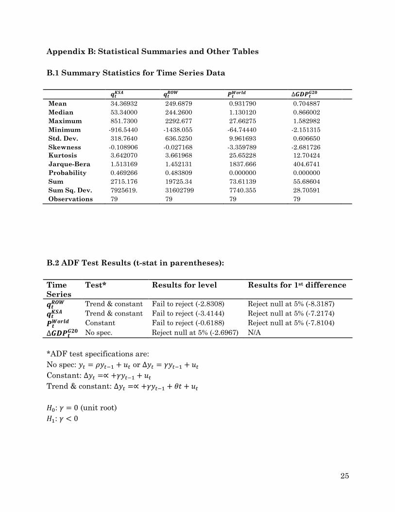
between 1994 and 2013. The non-stationarity of this series is reflected in failure to

reject the null hypothesis of a unit root via an Augmented Dickey-Fuller (ADF)

test.15 Saudi production behaves markedly different displaying far larger

percentage swings in production. This reflects Saudi’s role in world oil markets as a

swing producer actively targeting price. Nevertheless total additions of 3 million

bpd over the sample period fail to belie the presence of a unit root identified in the

series vis-à-vis an ADF test.

The real price series demonstrates a positive trend, especially as concerns the

increase in the per-barrel price after the year 2000, reflecting structural change in

world oil markets. This structural change is hypothesized to occur as a consequence

of consistent increases in the marginal cost of barrels outside of OPEC and other

large conventional reserve regions, serving new demand growth (Hamilton, 2014).

An ADF test rejects the null hypothesis of no unit root in the series.

14 Note: The statistical summaries are provided for 1st differenced data for those series found to be

non-stationary. See subsection 4.1. 15 Complete descriptions of test results for each series are available in Appendix B.2.

8

The identification of the stationarity of the % change in G20 (minus KSA) data

series rules out the possibility of estimating a vector error correction model (VECM)

as our set of series are not integrated of the same order.16 Instead, all series except

the I(0) process are transformed by taking first differences before estimating the

VAR.

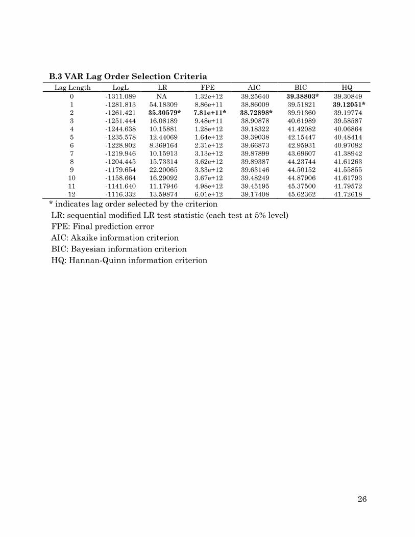
According to VAR lag order selection criteria and allowing for the possibility of up to

12 lags (12 quarters) we find the recommended optimal lag specification of 3

quarters according to sequential modified LR test statistic (each test at 5% level),

FPE (final prediction error) and the AIC (Akaike Information Criterion).17

Identification beyond restrictions on lag length includes restrictions on the entry of

contemporaneous interactions into the VAR structure to sort out causality,

introduced in the following section.

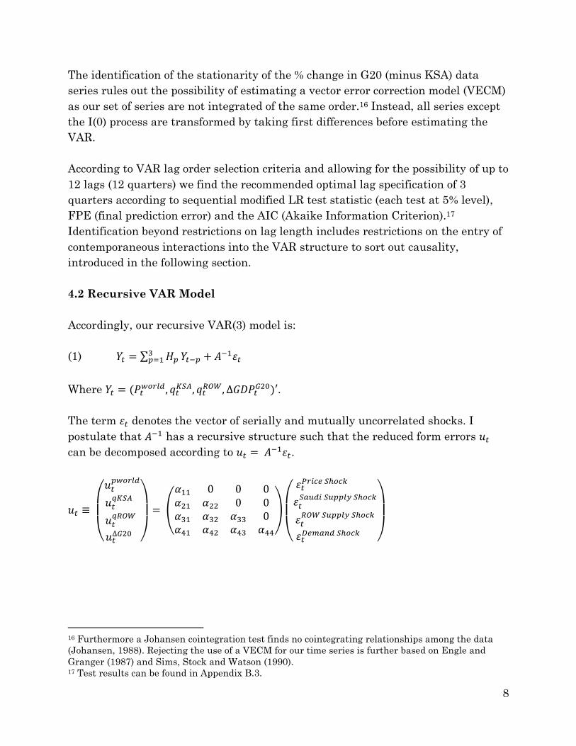
4.2 Recursive VAR Model

Accordingly, our recursive VAR(3) model is:

(1) 𝑌𝑡 = ∑ 𝐻𝑝3𝑝=1 𝑌𝑡−𝑝 + 𝐴

−1𝜀𝑡

Where 𝑌𝑡 = (𝑃𝑡𝑤𝑜𝑟𝑙𝑑, 𝑞𝑡

𝐾𝑆𝐴, 𝑞𝑡𝑅𝑂𝑊, ∆𝐺𝐷𝑃𝑡

𝐺20)′.

The term 𝜀𝑡 denotes the vector of serially and mutually uncorrelated shocks. I

postulate that 𝐴−1 has a recursive structure such that the reduced form errors 𝑢𝑡

can be decomposed according to 𝑢𝑡 = 𝐴−1𝜀𝑡.

𝑢𝑡 ≡

(

𝑢𝑡𝑝𝑤𝑜𝑟𝑙𝑑

𝑢𝑡𝑞𝐾𝑆𝐴

𝑢𝑡𝑞𝑅𝑂𝑊

𝑢𝑡∆𝐺20 )

= (

𝛼11 0 0 0𝛼21 𝛼22 0 0𝛼31 𝛼32 𝛼33 0𝛼41 𝛼42 𝛼43 𝛼44

)

(

𝜀𝑡𝑃𝑟𝑖𝑐𝑒 𝑆ℎ𝑜𝑐𝑘

𝜀𝑡𝑆𝑎𝑢𝑑𝑖 𝑆𝑢𝑝𝑝𝑙𝑦 𝑆ℎ𝑜𝑐𝑘

𝜀𝑡𝑅𝑂𝑊 𝑆𝑢𝑝𝑝𝑙𝑦 𝑆ℎ𝑜𝑐𝑘

𝜀𝑡𝐷𝑒𝑚𝑎𝑛𝑑 𝑆ℎ𝑜𝑐𝑘

)

16 Furthermore a Johansen cointegration test finds no cointegrating relationships among the data

(Johansen, 1988). Rejecting the use of a VECM for our time series is further based on Engle and

Granger (1987) and Sims, Stock and Watson (1990). 17 Test results can be found in Appendix B.3.

9

As a VAR can be considered to be the reduced form of a dynamic structural equation

(DSE) model, choosing 𝐴−1 is equivalent to imposing a recursive structure on the

corresponding DSE model.18 Following Kilian (2008) a recursive identification

structure is ordered based on assumptions regarding how quickly the different

variables respond.19 The ordering of the variables in 𝑌𝑡 (where also the matrix 𝐴−1 is

argued to be lower triangular) is based on the assumption that benchmark prices

for oil, reflecting the value of the marginal barrel, is taken to be the most quickly

updated variable in the system being the outcome of trades covering spot and

forward markets. Saudi Arabia, in contrast to ROW producers, quickly responds to

the price environment maintaining swing production capacity for this purpose.20

ROW producers, while certainly responsive to the price environment, react as more

conventional business entities hence responding more slowly than the OPEC cartel-

leader who is actively targeting price. Finally, as is documented by Hamilton (1983,

2003), GDP responds relatively sluggishly to oil price changes, hence occupies the

last place in the recursive structure.

5. Empirical Results

The model estimates are summarized in the following three sub-sections with

Granger-causality tests reported in 5.1, impulse responses functions (IRFs) in 5.2

and forecast error variance decompositions (FEVDs) reported in 5.3. Following

Stock and Watson (2001), these statistics are taken to be more informative than the

estimated VAR regression coefficients or 𝑅2statistics given the complicated

dynamics in the VAR.

5.1 Granger-Causality Statistics

Causality as defined by Granger (1969) is dealt with in the context of the estimated

VAR(3). The idea being if series 1 affects series 2, the former should help improving

the predictions of the latter variable. Granger causality thus reflects predictive

causality (as opposed to ‘real’ causality) given past values of the interrelated time

series. The null hypothesis in the following test results is that the lagged regressors

(three lags taken together) do not help predict the dependent variable in the

regression. 18 The centrality of the identification problem for sound empirical interpretation of estimation results

warrants a summary discussion of some of the mathematics of the Cholesky decomposition and its

relation to structural VARs which is hence provided in section D of the Appendix. 19 For brevity we will at times refer to the recursive identification structure imposed on the VAR as

the ‘Wold causal ordering’. See Appendix D for more information. 20 The response of Saudi swing production to price movement is further analyzed in Appendix A.3.

10

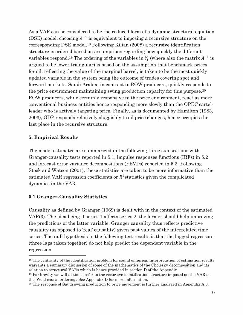
Table 5.1: Granger Causality Tests | Regressors (lag 3), 𝜒(76)2 test p-values reported

Dependent Variable 𝑷𝒕𝑾𝒐𝒓𝒍𝒅 𝒒𝒕

𝑲𝑺𝑨 𝒒𝒕𝑹𝑶𝑾 ∆𝑮𝑫𝑷𝒕

𝑮𝟐𝟎 All21

𝑷𝒕𝑾𝒐𝒓𝒍𝒅 N/A .99 .98 .01* .17

𝒒𝒕𝑲𝑺𝑨 .00* N/A .25 .94 .00*

𝒒𝒕𝑹𝑶𝑾 .11 .25 N/A .00* .00*

∆𝑮𝑫𝑷𝒕𝑮𝟐𝟎 .00* .78 .94 N/A .00*

The results in Table 5.1 suggest GDP helps to predict price, but that production in

KSA and ROW do not help to predict price. Price helps to predict KSA production

but ROW production and GDP do not help to predict KSA production. Neither price

nor KSA production help to predict ROW production. GDP however does help to

predict ROW production. Finally, price helps to predict GDP but KSA and ROW

production does not. Only production in KSA and ROW, as well as GDP, treated

jointly fails to predict price yielding a p-value equal to .17 versus .00 for the other

joint tests.

5.2 Orthoganalized IRFs: Dynamic Responses

Granger-causality may not tell us the complete story about the interactions between

the variables in the system. It is therefore of interest to know the time path

response of one variable to an impulse in another variable in the 4-dimensional oil

market system. Beyond estimated coefficients, impulse response functions or IRFs

show the size of the impact of the shock plus the rate at which the shock dissipates,

allowing for interdependencies.22 The dynamic character of the oil system has

motivated the VAR specification and as such is substantively analyzed in context of

IRFs.

Simple IRFs have a drawback in that they give the effect over time of a one-time

unit increase to one of the shocks, holding all else constant. But to the extent the

shocks are contemporaneously correlated, the other shocks cannot be held constant,

adversely affecting the causal interpretation of the VAR model. This drawback is

overcome with the recursive identification structure or Wold causal ordring

introduced in subsection 4.2 which yields orthoganalized IRFs (See Appendix D for

a more extensive discussion).

21 The statistic in the last column (All) is the statistic for joint significance of all other lagged

endogenous variables in the equation. 22 Shock here is defined as a one S.D. innovation with the error bands denoting ±2 S.E.

11

Further, for IRFs to be computed, the VAR must be stable. Tests reveal the inverse

roots of the characteristic AR polynomial are all less than 1 ensuring stability of the

estimated model. Given the importance of stability conditions for our empirical

results, Appendix C expands on VAR(3) stability.

As expected, Saudi Arabia responds to price within one quarter by increasing

production as seen in the left panel of figure 5.1. Production increases yet again

before leveling off and decreasing by the 4th quarter. There is no evidence of

persistence which is consistent with Saudi role of continually adjusting production

to target the price level.

Figure 5.1: Production responses to price shocks.

The immediate effect of a shock in price to ROW production appears to initially

decrease followed by a two period increase, continuing a dampening and mildly

oscillating pattern before the effect is eliminated. Lagged response in ROW

production may reflect the time required to realize new production after making

decisions related to new capital expenditures.

Saudi control over the price level is, by definition of the recursive scheme imposed

on the VAR, zero in the first period as seen in the left panel of figure 5.2. Beyond

that the time path of price response moves below zero (by period 3) for several

periods before the effect dies out, suggesting that Saudi supply affects price with a 3

period lag persisting for several quarters. Intuitively, inventory accumulation can

be hypothesized to delay the period in which Saudi production swings can affect

price which may explain the 3 period delay in response.

-200

-100

0

100

200

300

400

1 2 3 4 5 6 7 8 9 10 11 12

Response of DQ_KSA to DREAL_P_WORLD

-400

-200

0

200

400

600

800

1 2 3 4 5 6 7 8 9 10 11 12

Response of DQ_ROW to DREAL_P_WORLD

12

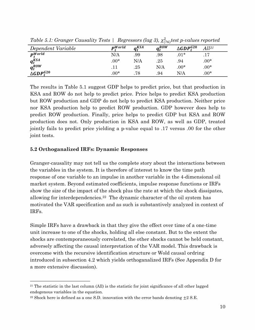
Figure 5.2: Price level responses to production shocks.

A positive shock in ROW production exercises no demonstrable effect on price as is

evidenced in the IRF in the left panel of figure 5.2.

Saudi production response to movements in ROW production is initially zero (due to

the ordering of contemporaneous relations) before increasing over the course of

three periods, mildly dipping below 0 in the sixth period. There is no persistence

evident. This response path may be due to ROW production responding to upward

movements in price with Saudi Arabia following.

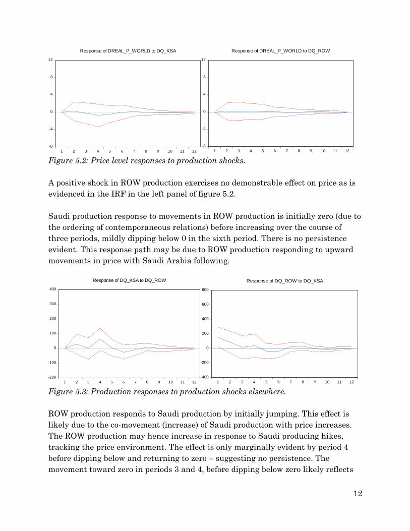
Figure 5.3: Production responses to production shocks elsewhere.

ROW production responds to Saudi production by initially jumping. This effect is

likely due to the co-movement (increase) of Saudi production with price increases.

The ROW production may hence increase in response to Saudi producing hikes,

tracking the price environment. The effect is only marginally evident by period 4

before dipping below and returning to zero – suggesting no persistence. The

movement toward zero in periods 3 and 4, before dipping below zero likely reflects

-8

-4

0

4

8

12

1 2 3 4 5 6 7 8 9 10 11 12

Response of DREAL_P_WORLD to DQ_KSA

-8

-4

0

4

8

12

1 2 3 4 5 6 7 8 9 10 11 12

Response of DREAL_P_WORLD to DQ_ROW

-200

-100

0

100

200

300

400

1 2 3 4 5 6 7 8 9 10 11 12

Response of DQ_KSA to DQ_ROW

-400

-200

0

200

400

600

800

1 2 3 4 5 6 7 8 9 10 11 12

Response of DQ_ROW to DQ_KSA

13

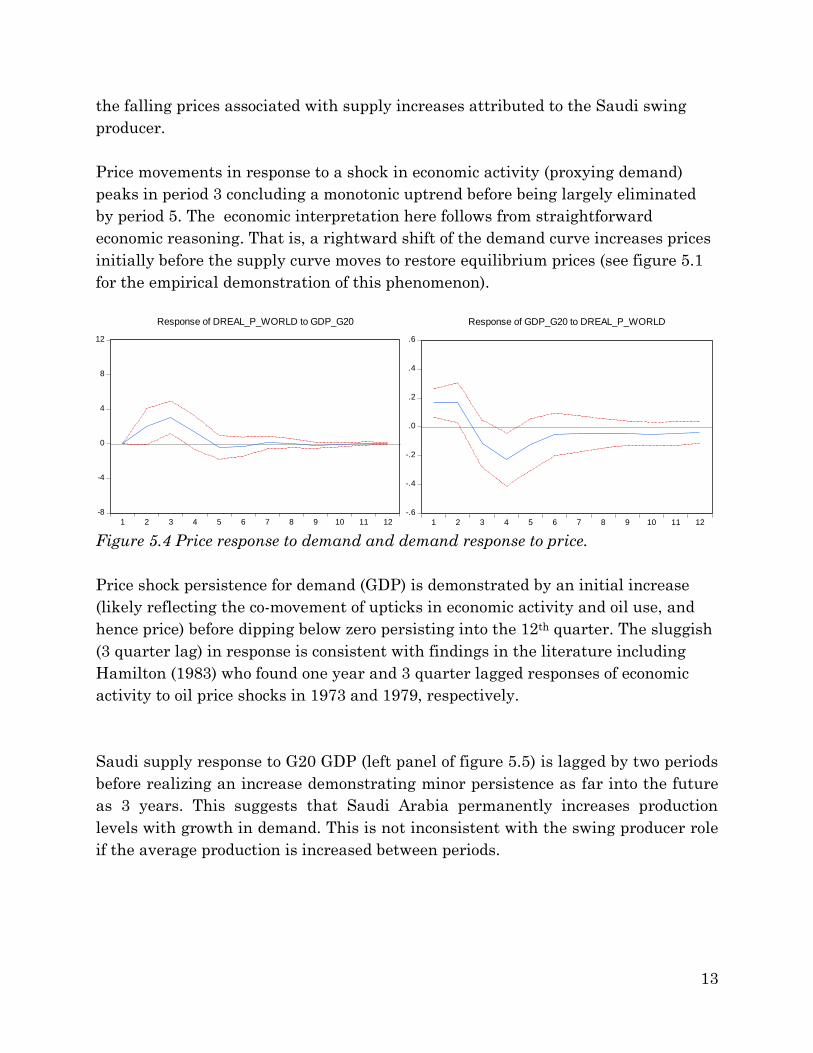
the falling prices associated with supply increases attributed to the Saudi swing

producer.

Price movements in response to a shock in economic activity (proxying demand)

peaks in period 3 concluding a monotonic uptrend before being largely eliminated

by period 5. The economic interpretation here follows from straightforward

economic reasoning. That is, a rightward shift of the demand curve increases prices

initially before the supply curve moves to restore equilibrium prices (see figure 5.1

for the empirical demonstration of this phenomenon).

Figure 5.4 Price response to demand and demand response to price.

Price shock persistence for demand (GDP) is demonstrated by an initial increase

(likely reflecting the co-movement of upticks in economic activity and oil use, and

hence price) before dipping below zero persisting into the 12th quarter. The sluggish

(3 quarter lag) in response is consistent with findings in the literature including

Hamilton (1983) who found one year and 3 quarter lagged responses of economic

activity to oil price shocks in 1973 and 1979, respectively.

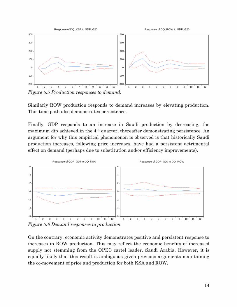
Saudi supply response to G20 GDP (left panel of figure 5.5) is lagged by two periods

before realizing an increase demonstrating minor persistence as far into the future

as 3 years. This suggests that Saudi Arabia permanently increases production

levels with growth in demand. This is not inconsistent with the swing producer role

if the average production is increased between periods.

-8

-4

0

4

8

12

1 2 3 4 5 6 7 8 9 10 11 12

Response of DREAL_P_WORLD to GDP_G20

-.6

-.4

-.2

.0

.2

.4

.6

1 2 3 4 5 6 7 8 9 10 11 12

Response of GDP_G20 to DREAL_P_WORLD

14

Figure 5.5 Production responses to demand.

Similarly ROW production responds to demand increases by elevating production.

This time path also demonstrates persistence.

Finally, GDP responds to an increase in Saudi production by decreasing, the

maximum dip achieved in the 4th quarter, thereafter demonstrating persistence. An

argument for why this empirical phenomenon is observed is that historically Saudi

production increases, following price increases, have had a persistent detrimental

effect on demand (perhaps due to substitution and/or efficiency improvements).

Figure 5.6 Demand responses to production.

On the contrary, economic activity demonstrates positive and persistent response to

increases in ROW production. This may reflect the economic benefits of increased

supply not stemming from the OPEC cartel leader, Saudi Arabia. However, it is

equally likely that this result is ambiguous given previous arguments maintaining

the co-movement of price and production for both KSA and ROW.

-200

-100

0

100

200

300

400

1 2 3 4 5 6 7 8 9 10 11 12

Response of DQ_KSA to GDP_G20

-400

-200

0

200

400

600

800

1 2 3 4 5 6 7 8 9 10 11 12

Response of DQ_ROW to GDP_G20

-.6

-.4

-.2

.0

.2

.4

.6

1 2 3 4 5 6 7 8 9 10 11 12

Response of GDP_G20 to DQ_KSA

-.6

-.4

-.2

.0

.2

.4

.6

1 2 3 4 5 6 7 8 9 10 11 12

Response of GDP_G20 to DQ_ROW

15

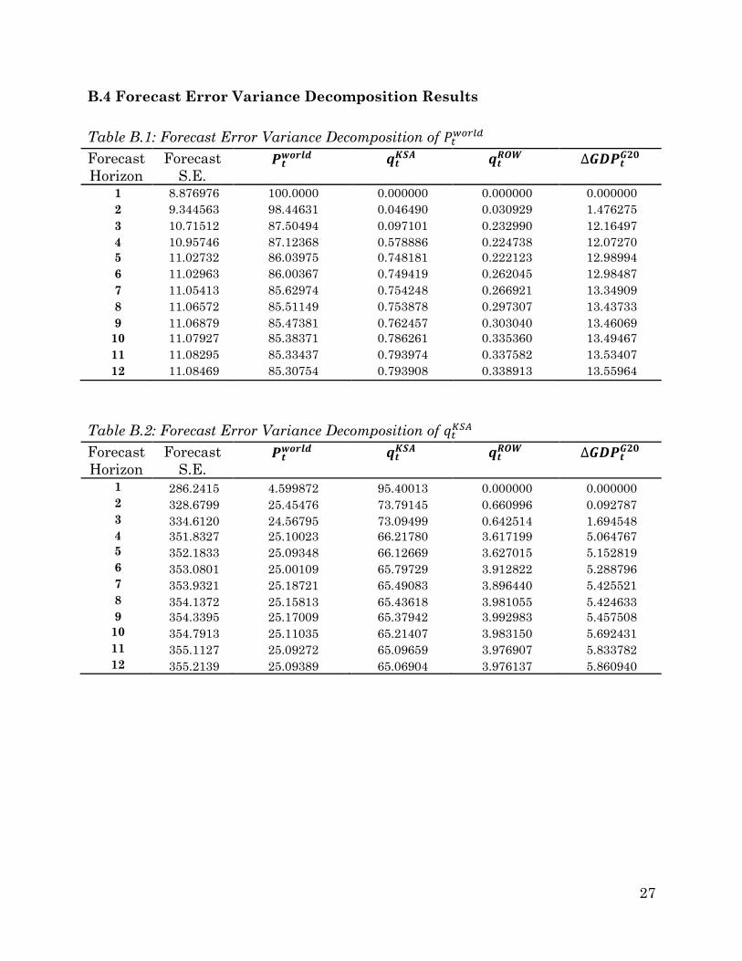
5.3 Forecast Error Variance Decomposition

The idea behind constructing forecast error variance decompositions or FEVD is to

determine the proportion of the variability of the errors in forecasting 𝑌𝑡 at time

𝑡 + 𝑠 based on information available at time 𝑡 that is due to variability in the

structural shocks 𝜀𝑡 between times 𝑡 and 𝑡 + 𝑠. The typical use of the variance

decomposition is to make statements regarding the percentage of the variance

explained by innovations/shocks in a given variable. Just as when we discussed

IRFs, this statement is only sensible if we can attach some structural meaning to

the shock under consideration. Thus identification of the structural shocks requires

the same assumptions imposed on the transformation matrix A as we made in the

preceding sections. The 4 charts below display FEVD results for 𝑃𝑡𝑤𝑜𝑟𝑙𝑑 , 𝑞𝑡

𝐾𝑆𝐴, 𝑞𝑡𝑅𝑂𝑊

and ∆𝐺𝐷𝑃𝑡𝐺20. What is striking is the dominance of two variables in each case for

explaining the said forecast error.23 The primacy of 2 variables in each FEVD is

consistent with the Granger causality statistics computed in subsection 5.1 in so far

as only 1 variable (excluding itself) was found to predictively cause the associated

dependent variable. The consistency across time of the relative proportions of

explained forecast error variance is nearly constant in all 4 FEVDs after

approximately the 3rd or 4th period.

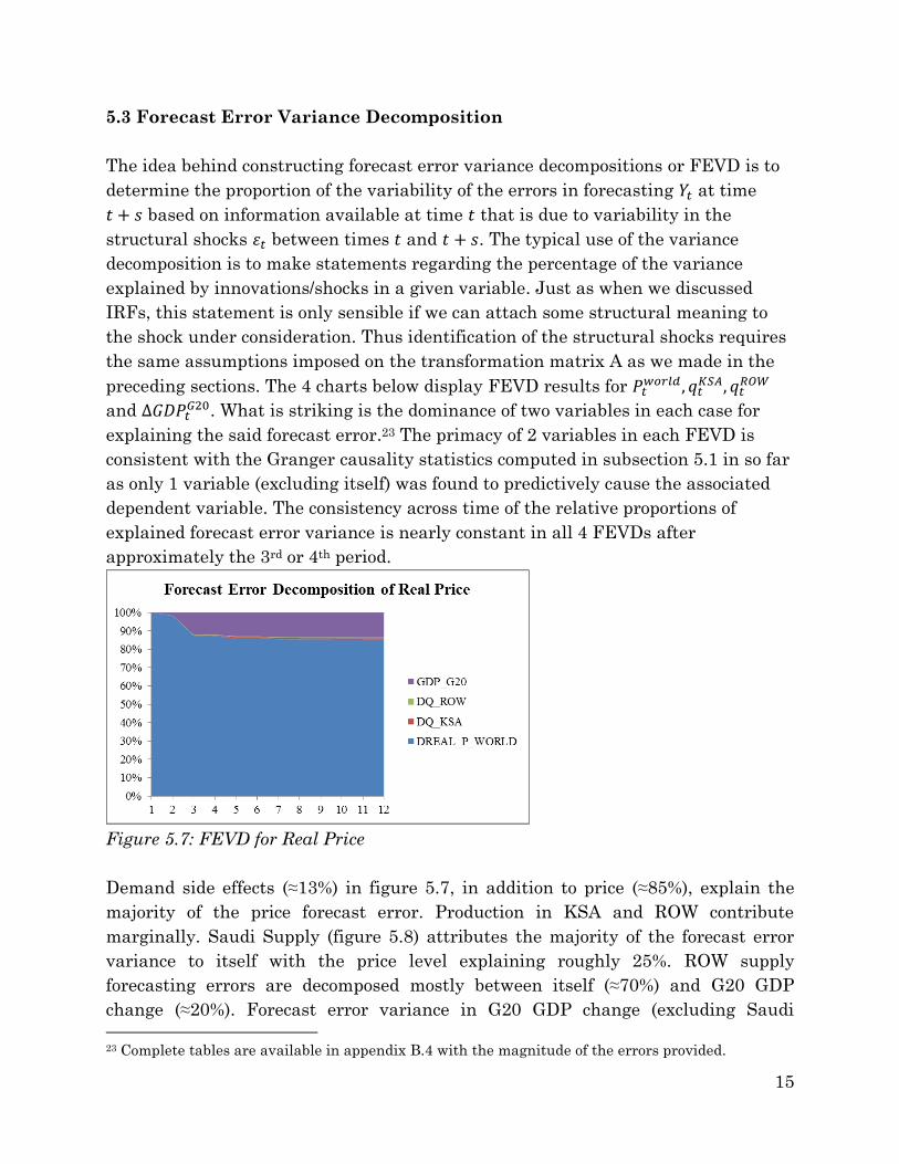
Figure 5.7: FEVD for Real Price

Demand side effects (≈13%) in figure 5.7, in addition to price (≈85%), explain the

majority of the price forecast error. Production in KSA and ROW contribute

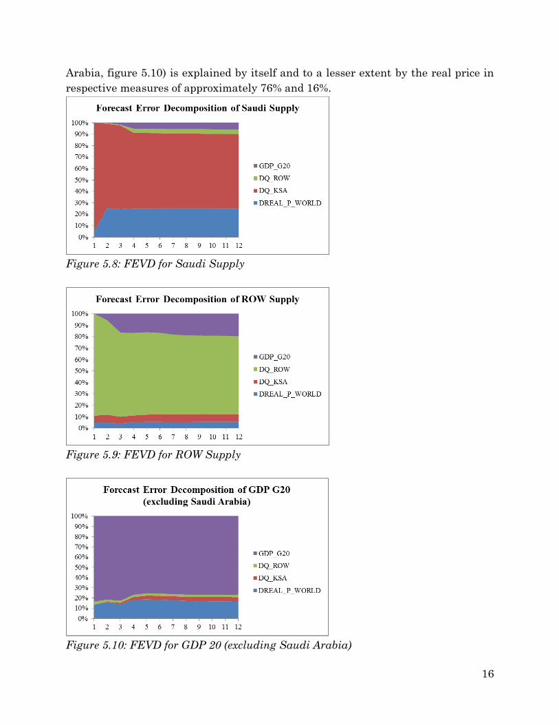
marginally. Saudi Supply (figure 5.8) attributes the majority of the forecast error

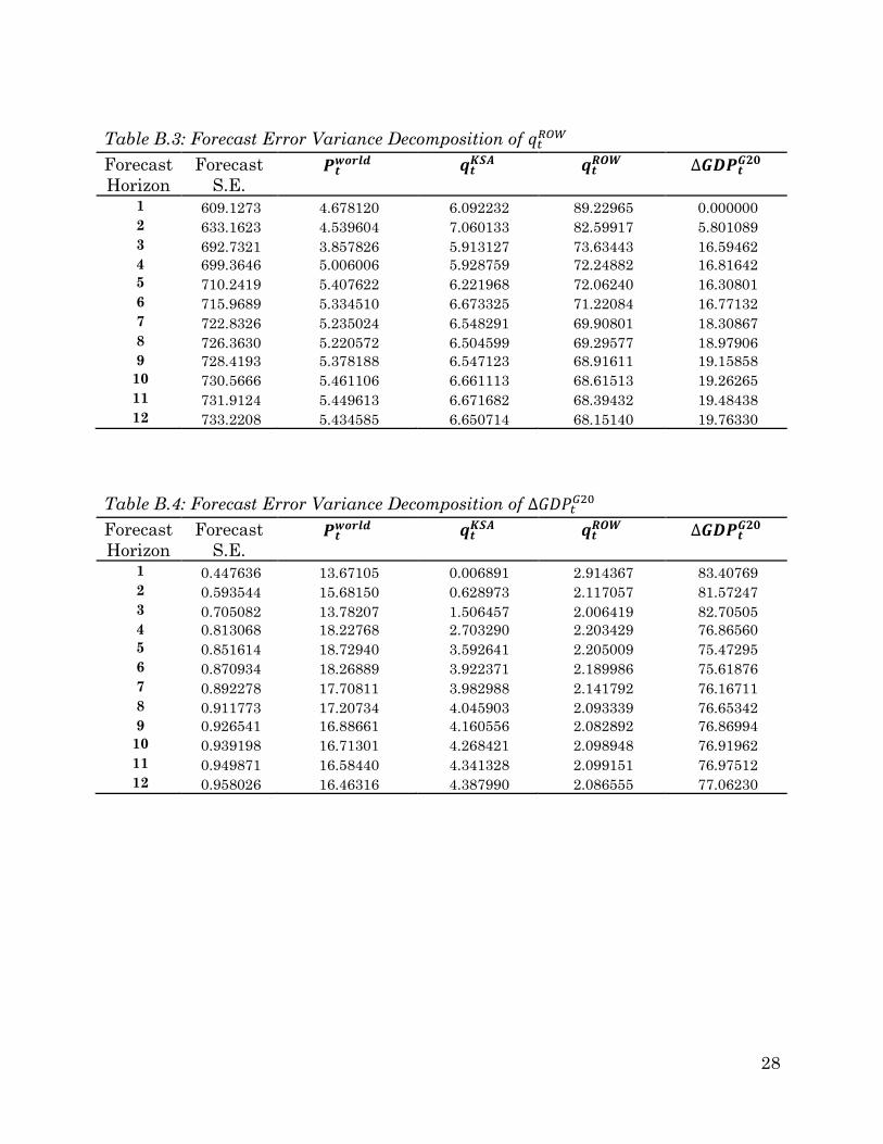
variance to itself with the price level explaining roughly 25%. ROW supply

forecasting errors are decomposed mostly between itself (≈70%) and G20 GDP

change (≈20%). Forecast error variance in G20 GDP change (excluding Saudi

23 Complete tables are available in appendix B.4 with the magnitude of the errors provided.

16

Arabia, figure 5.10) is explained by itself and to a lesser extent by the real price in

respective measures of approximately 76% and 16%.

Figure 5.8: FEVD for Saudi Supply

Figure 5.9: FEVD for ROW Supply

Figure 5.10: FEVD for GDP 20 (excluding Saudi Arabia)

17

6. Tentative Conclusions

The central pillar of the research approach taken here maintains that Saudi Arabia

generates unique data points in the oil production space, given its unique presence

in the international oil order. Its role in world oil was hence empirically evaluated

in context of a vector autoregression, separating out Saudi production from the

remainder of the production space. However, given the numerous dynamic

interrelations characterizing the multivariate model, no specific hypotheses were

advanced. Rather the research emphasis has been on observing estimated Granger

causality statistics, the time paths produced through the IRFs, and FEVDs for all

variables in a system deemed to be relevant for modeling oil market reality.

Nevertheless, the empirical findings, especially as concerns the time paths obtained

through the IRFs, suggest that certain questions can be asked of the data upon

conclusion with regard to Saudi supply. Of particular interest are questions related

to the dynamic responses of production reflecting medium term, i.e. investment-

cycle effects given their importance in offsetting field decline and expanding

capacity to meet future market demand. It was found that Saudi production

demonstrates persistence in response to shocks in demand. However, no persistence

was demonstrated in response to shocks stemming from production increases in the

remainder of the production space – or from price increases. The practical

implication suggests that Saudi Arabia responds with long run responses to demand

changes but no long run consequences arise from production movements outside of

Saudi Arabia. Surprisingly, no long run consequences regarding Saudi production

are found to arise from price shocks.

The price level has figured prominently in all these statistical tests. This reflects its

place within the Wold causal ordering imposed on the VAR but also its central

importance to all variable movements in the estimated system. ∆𝐺𝐷𝑃𝑡𝐺20, serving as

a proxy for demand has also been an influential variable in our empirical findings.

The supply side on the other hand has been less important reflecting perhaps the

relative stability of energy supplies over the sample period. Potential caveats can

include (1) potentially faulty identification in the Wold causal ordering and (2)

whether the estimated model is inclusive of oil market reality (omitted variable

bias, incorrectly specified lag length). Nevertheless, variable inclusion is based on

careful consideration of oil markets and lag length is selected on the basis of well-

regarded statistical tests. The recursive ordering is similarly introduced on the

basis of careful consideration of the oil markets and the oil industry.

18

7. References

Adelman, M. (1980), “The Clumsy Cartel”, The Energy Journal Vol. 1

Adelman, M. (1982), “OPEC as a Cartel”, in OPEC Behavior and World Oil Price

London: Allen & Unwin

Al-Kasim, F. (2006), “Managing Petroleum Resources: The Norwegian Model in a

Broad Perspective”, Oxford Institute for Energy Studies, Publication

Carruth, A., Hooker, M., and Oswald, A. (1998), “Unemployment Equilibria and

Input Prices: Theory and Evidence from the United States,” Review of

Economics and Statistics 80

Daniel, B. (1997), “International Interdependence of National Growth Rates: A

Structural Trends Analysis,” Journal of Monetary Economics 40

Engle, F. and Granger, C., (1987), “Co-integration and Error Correction:

Representation, Estimation and Testing”, Econometrica Vol. 55

EIA (2014), “Country Analysis Brief: Saudi Arabia” Washington, DC

“Country Analysis Brief: Iran” Washington, DC

Johansen, S. (1988), “Statistical Analysis of Cointegrating Vectors”, Journal of

Economic Dynamics and Control, Vol. 12

Hnyilicza, E. and Pindyck, R. (1976), “Pricing Policies for a Two-Part Exhaustible

Resource Cartel: The Case of OPEC” European Economic Review Vol. 8

Fattouh, B. (2006), “The Origons and Evolution of the Current International Oil

Pricing System: A Critical Assessment” in Oil in the Twenty First Century:

Issues, Challenges, and Opportunities. Oxford: Oxford University Press

Fattouh, B. (2007), “OPEC Pricing Power: The Need for a New Perspective”, Oxford

Institute for Energy Studies, Oxford

Fattouh, B. (2011), “An Anatomy of the Crude Oil Pricing System”, Oxford Institute

for Energy Studies, Oxford

19

Granger, C. (1969), “Investigating Causal Relations by Econometric Models and

Crossspectral Methods”, Econometrica, Vol. 37, No. 3

Hamilton, J. D. (1983), “Oil and the Macroeconomy since World War II”, The

Journal of Political Economy Vol. 91

Hamilton, J. D. (1994). “Time Series Analysis”, Princeton University Press

Hamilton, J. D. (2003), “What is an Oil Shock”, Journal of Econometrics Vol. 113

Hamilton, J. D. (2014), “The Changing Face of World Oil Markets”, Working Paper

IEA (2011), “Overseas Investments by Chinese National Oil Companies: Assessing

the Drivers and Impacts”, International Energy Agency, Paris

IEA (2013), “World Energy Outlook 2013”: International Energy Agency, Paris

IEA (2014), “Medium Term Oil Market Report 2014”: International Energy Agency,

Paris

Kilian, L. (2008), “Not all Oil Price Shocks Are Alike: Disentangling Demand and

Supply Shocks in the Crude Oil Market”, Working Paper

Kshirsagar, A. (1962), “Prediction from Simultaneous Equation Systems and Wold’s

Implicit Casual Chain Model”, Econometrica, Vol. 30

Lütkepohl, H. (2005) “New Introduction to Multiple Time Series Analysis”,

Springer.

Mabro, R. (1998), “OPEC Behavior 1960-1998: A Review of the Literature”, The

Journal of Energy Literature

Moody’s (2003), “Petroleos Mexicanos (PEMEX): Lack of Fiscal Autonomy

Constrains Production Growth and Raises Financial Leverage.” Special

Comment, Moody’s Investor Service

Salant, S. (1976) “Exhaustible Resources and Industrial Structure: A Nash-Cournot

Approach to the World Oil Market”, Journal of Political Economy Vol. 84

20

Sims, C. A., (1980a), “Comparison of Interwar and Postwar Business Cycles:

Monetarism Reconsidered”, American Economic Review Vol. 70

Sims, C. A., (1980b), “Macroeconomics and Reality”, Econometrica Vol. 48

Sims, C. A., (1986), “Are Forecasting Models Usable for Policy Analysis?”,

Minneapolis Federal Reserve Bank Quarterly Review Vol. 10

Sims, C. A., (1992), “Interpreting the Macroeconomic Time Series Facts: The Effect

of Monetary Policy”, European Economic Review Vol. 36

Sims, C. A., Stock, J., and Watson, M., (1990), “Inference in Linear Time Series

Models with Some Unit Roots”, Econometrica Vol. 58

Smith, J. (2005), “Inscrutable OPEC? Behavioral Tests of the Cartel Hypothesis”,

The Energy Journal Vol. 16

Stevens, P. (2008), “A Methodology for Assessing the Performance of National Oil

Companies.” Background Paper for a Study on National Oil Companies and

Value Creation, World Bank, Washington DC

Stock, J. and Watson, M. (2001), “Vector Autoregressions”, Journal of Economic

Perspectives, Vol. 15, No. 4

Terzian, P., (1985), “OPEC: The Inside Story”, London: Zed Books

Tordo, S. (2011), “National Oil Companies and Value Creation” Working Paper

No. 218, World Bank, Washington DC

Victor, N. (2008), “Gazprom: Gas Giant under Strain” Working Paper 71, Program

on Energy and Sustainable Development, Stanford University

Wold, H. (1960), “A Generalization of Causal Chain Models”, Econometrica, Vol. 28

21

8. Appendices

Appendix A: Select Time Series and Other Charts

A.1 The Data

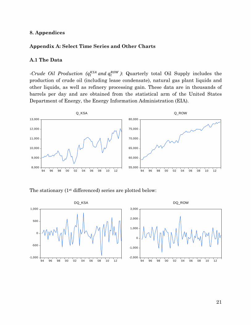
-Crude Oil Production (𝑞𝑡𝐾𝑆𝐴 𝑎𝑛𝑑 𝑞𝑡

𝑅𝑂𝑊 ): Quarterly total Oil Supply includes the

production of crude oil (including lease condensate), natural gas plant liquids and

other liquids, as well as refinery processing gain. These data are in thousands of

barrels per day and are obtained from the statistical arm of the United States

Department of Energy, the Energy Information Administration (EIA).

The stationary (1st differenced) series are plotted below:

8,000

9,000

10,000

11,000

12,000

13,000

94 96 98 00 02 04 06 08 10 12

Q_KSA

55,000

60,000

65,000

70,000

75,000

80,000

94 96 98 00 02 04 06 08 10 12

Q_ROW

-1,000

-500

0

500

1,000

94 96 98 00 02 04 06 08 10 12

DQ_KSA

-2,000

-1,000

0

1,000

2,000

3,000

94 96 98 00 02 04 06 08 10 12

DQ_ROW

22

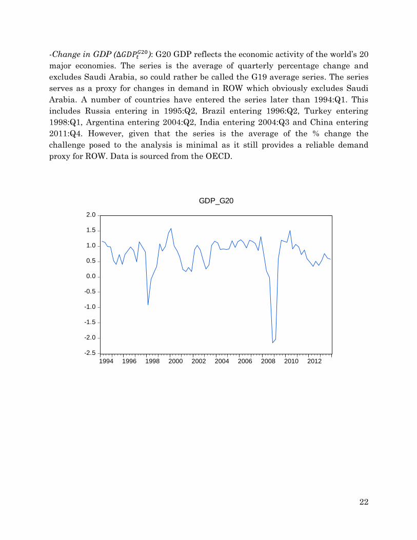
-Change in GDP (∆𝐺𝐷𝑃𝑡𝐺20): G20 GDP reflects the economic activity of the world’s 20

major economies. The series is the average of quarterly percentage change and

excludes Saudi Arabia, so could rather be called the G19 average series. The series

serves as a proxy for changes in demand in ROW which obviously excludes Saudi

Arabia. A number of countries have entered the series later than 1994:Q1. This

includes Russia entering in 1995:Q2, Brazil entering 1996:Q2, Turkey entering

1998:Q1, Argentina entering 2004:Q2, India entering 2004:Q3 and China entering

2011:Q4. However, given that the series is the average of the % change the

challenge posed to the analysis is minimal as it still provides a reliable demand

proxy for ROW. Data is sourced from the OECD.

-2.5

-2.0

-1.5

-1.0

-0.5

0.0

0.5

1.0

1.5

2.0

1994 1996 1998 2000 2002 2004 2006 2008 2010 2012

GDP_G20

23

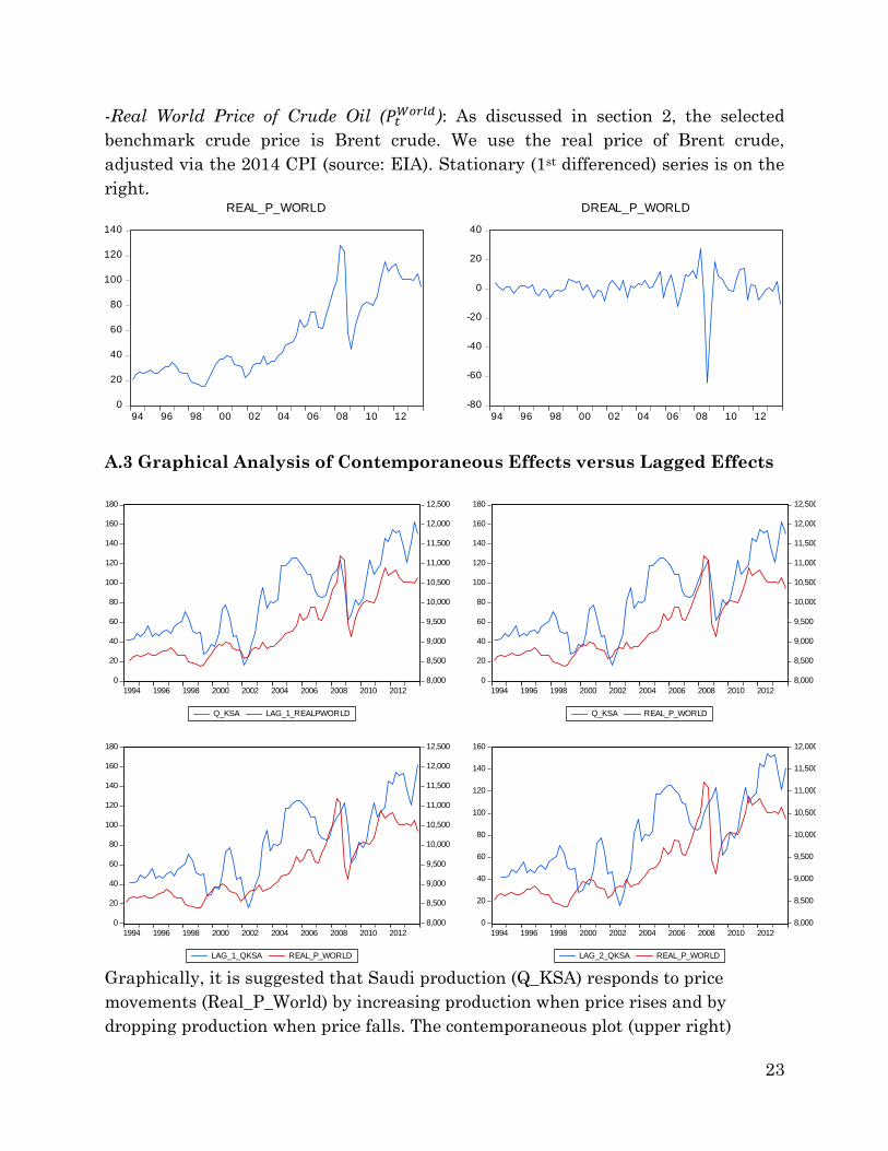
-Real World Price of Crude Oil (𝑃𝑡𝑊𝑜𝑟𝑙𝑑): As discussed in section 2, the selected

benchmark crude price is Brent crude. We use the real price of Brent crude,

adjusted via the 2014 CPI (source: EIA). Stationary (1st differenced) series is on the

right.

A.3 Graphical Analysis of Contemporaneous Effects versus Lagged Effects

Graphically, it is suggested that Saudi production (Q_KSA) responds to price

movements (Real_P_World) by increasing production when price rises and by

dropping production when price falls. The contemporaneous plot (upper right)

0

20

40

60

80

100

120

140

94 96 98 00 02 04 06 08 10 12

REAL_P_WORLD

-80

-60

-40

-20

0

20

40

94 96 98 00 02 04 06 08 10 12

DREAL_P_WORLD

0

20

40

60

80

100

120

140

160

180

8,000

8,500

9,000

9,500

10,000

10,500

11,000

11,500

12,000

12,500

1994 1996 1998 2000 2002 2004 2006 2008 2010 2012

Q_KSA LAG_1_REALPWORLD

0

20

40

60

80

100

120

140

160

180

8,000

8,500

9,000

9,500

10,000

10,500

11,000

11,500

12,000

12,500

1994 1996 1998 2000 2002 2004 2006 2008 2010 2012

Q_KSA REAL_P_WORLD

0

20

40

60

80

100

120

140

160

180

8,000

8,500

9,000

9,500

10,000

10,500

11,000

11,500

12,000

12,500

1994 1996 1998 2000 2002 2004 2006 2008 2010 2012

LAG_1_QKSA REAL_P_WORLD

0

20

40

60

80

100

120

140

160

8,000

8,500

9,000

9,500

10,000

10,500

11,000

11,500

12,000

1994 1996 1998 2000 2002 2004 2006 2008 2010 2012

LAG_2_QKSA REAL_P_WORLD

24

suggests production tracks price with a lag of one. Furthermore, lagging price by

one period appears to show production tracking price contemporaneously (upper left

plot). The economic interpretation of this is that Saudi production seeks to increase

revenues on price increases and boost prices during downturns, but cannot respond

instantaneously. The graphical analysis suggests production follows price and not

the other way around, informing our choice of setting price as the first causal

variable in the recursive structure.

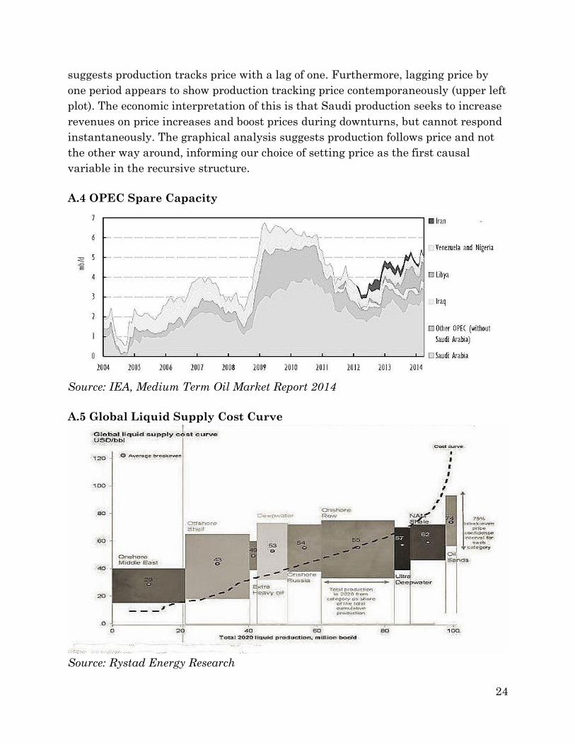
A.4 OPEC Spare Capacity

Source: IEA, Medium Term Oil Market Report 2014

A.5 Global Liquid Supply Cost Curve

Source: Rystad Energy Research

25

Appendix B: Statistical Summaries and Other Tables

B.1 Summary Statistics for Time Series Data

𝒒𝒕𝑲𝑺𝑨 𝒒𝒕

𝑹𝑶𝑾 𝑷𝒕𝑾𝒐𝒓𝒍𝒅 ∆𝑮𝑫𝑷𝒕

𝑮𝟐𝟎

Mean 34.36932 249.6879 0.931790 0.704887

Median 53.34000 244.2600 1.130120 0.866002

Maximum 851.7300 2292.677 27.66275 1.582982

Minimum -916.5440 -1438.055 -64.74440 -2.151315

Std. Dev. 318.7640 636.5250 9.961693 0.606650

Skewness -0.108906 -0.027168 -3.359789 -2.681726

Kurtosis 3.642070 3.661968 25.65228 12.70424

Jarque-Bera 1.513169 1.452131 1837.666 404.6741

Probability 0.469266 0.483809 0.000000 0.000000

Sum 2715.176 19725.34 73.61139 55.68604

Sum Sq. Dev. 7925619. 31602799 7740.355 28.70591

Observations 79 79 79 79

B.2 ADF Test Results (t-stat in parentheses):

Time

Series

Test* Results for level Results for 1st difference

𝒒𝒕𝑹𝑶𝑾 Trend & constant Fail to reject (-2.8308) Reject null at 5% (-8.3187)

𝒒𝒕𝑲𝑺𝑨 Trend & constant Fail to reject (-3.4144) Reject null at 5% (-7.2174)

𝑷𝒕𝑾𝒐𝒓𝒍𝒅 Constant Fail to reject (-0.6188) Reject null at 5% (-7.8104)

∆𝑮𝑫𝑷𝒕𝑮𝟐𝟎 No spec. Reject null at 5% (-2.6967) N/A

*ADF test specifications are:

No spec: 𝑦𝑡 = 𝜌𝑦𝑡−1 + 𝑢𝑡 or ∆𝑦𝑡 = 𝛾𝑦𝑡−1 + 𝑢𝑡

Constant: ∆𝑦𝑡 =∝ +𝛾𝑦𝑡−1 + 𝑢𝑡

Trend & constant: ∆𝑦𝑡 =∝ +𝛾𝑦𝑡−1 + 𝜃𝑡 + 𝑢𝑡

𝐻0: 𝛾 = 0 (unit root)

𝐻1: 𝛾 < 0

26

B.3 VAR Lag Order Selection Criteria

Lag Length LogL LR FPE AIC BIC HQ

0 -1311.089 NA 1.32e+12 39.25640 39.38803* 39.30849

1 -1281.813 54.18309 8.86e+11 38.86009 39.51821 39.12051*

2 -1261.421 35.30579* 7.81e+11* 38.72898* 39.91360 39.19774

3 -1251.444 16.08189 9.48e+11 38.90878 40.61989 39.58587

4 -1244.638 10.15881 1.28e+12 39.18322 41.42082 40.06864

5 -1235.578 12.44069 1.64e+12 39.39038 42.15447 40.48414

6 -1228.902 8.369164 2.31e+12 39.66873 42.95931 40.97082

7 -1219.946 10.15913 3.13e+12 39.87899 43.69607 41.38942

8 -1204.445 15.73314 3.62e+12 39.89387 44.23744 41.61263

9 -1179.654 22.20065 3.33e+12 39.63146 44.50152 41.55855

10 -1158.664 16.29092 3.67e+12 39.48249 44.87906 41.61793

11 -1141.640 11.17946 4.98e+12 39.45195 45.37500 41.79572

12 -1116.332 13.59874 6.01e+12 39.17408 45.62362 41.72618

* indicates lag order selected by the criterion

LR: sequential modified LR test statistic (each test at 5% level)

FPE: Final prediction error

AIC: Akaike information criterion

BIC: Bayesian information criterion

HQ: Hannan-Quinn information criterion

27

B.4 Forecast Error Variance Decomposition Results

Table B.1: Forecast Error Variance Decomposition of 𝑃𝑡𝑤𝑜𝑟𝑙𝑑

Forecast

Horizon

Forecast

S.E. 𝑷𝒕𝒘𝒐𝒓𝒍𝒅

𝒒𝒕𝑲𝑺𝑨

𝒒𝒕𝑹𝑶𝑾

∆𝑮𝑫𝑷𝒕𝑮𝟐𝟎

1 8.876976 100.0000 0.000000 0.000000 0.000000

2 9.344563 98.44631 0.046490 0.030929 1.476275

3 10.71512 87.50494 0.097101 0.232990 12.16497

4 10.95746 87.12368 0.578886 0.224738 12.07270

5 11.02732 86.03975 0.748181 0.222123 12.98994

6 11.02963 86.00367 0.749419 0.262045 12.98487

7 11.05413 85.62974 0.754248 0.266921 13.34909

8 11.06572 85.51149 0.753878 0.297307 13.43733

9 11.06879 85.47381 0.762457 0.303040 13.46069

10 11.07927 85.38371 0.786261 0.335360 13.49467

11 11.08295 85.33437 0.793974 0.337582 13.53407

12 11.08469 85.30754 0.793908 0.338913 13.55964

Table B.2: Forecast Error Variance Decomposition of 𝑞𝑡𝐾𝑆𝐴

Forecast

Horizon

Forecast

S.E. 𝑷𝒕𝒘𝒐𝒓𝒍𝒅

𝒒𝒕𝑲𝑺𝑨

𝒒𝒕𝑹𝑶𝑾

∆𝑮𝑫𝑷𝒕𝑮𝟐𝟎

1 286.2415 4.599872 95.40013 0.000000 0.000000

2 328.6799 25.45476 73.79145 0.660996 0.092787

3 334.6120 24.56795 73.09499 0.642514 1.694548

4 351.8327 25.10023 66.21780 3.617199 5.064767

5 352.1833 25.09348 66.12669 3.627015 5.152819

6 353.0801 25.00109 65.79729 3.912822 5.288796

7 353.9321 25.18721 65.49083 3.896440 5.425521

8 354.1372 25.15813 65.43618 3.981055 5.424633

9 354.3395 25.17009 65.37942 3.992983 5.457508

10 354.7913 25.11035 65.21407 3.983150 5.692431

11 355.1127 25.09272 65.09659 3.976907 5.833782

12 355.2139 25.09389 65.06904 3.976137 5.860940

28

Table B.3: Forecast Error Variance Decomposition of 𝑞𝑡𝑅𝑂𝑊

Forecast

Horizon

Forecast

S.E. 𝑷𝒕𝒘𝒐𝒓𝒍𝒅

𝒒𝒕𝑲𝑺𝑨

𝒒𝒕𝑹𝑶𝑾

∆𝑮𝑫𝑷𝒕𝑮𝟐𝟎

1 609.1273 4.678120 6.092232 89.22965 0.000000

2 633.1623 4.539604 7.060133 82.59917 5.801089

3 692.7321 3.857826 5.913127 73.63443 16.59462

4 699.3646 5.006006 5.928759 72.24882 16.81642

5 710.2419 5.407622 6.221968 72.06240 16.30801

6 715.9689 5.334510 6.673325 71.22084 16.77132

7 722.8326 5.235024 6.548291 69.90801 18.30867

8 726.3630 5.220572 6.504599 69.29577 18.97906

9 728.4193 5.378188 6.547123 68.91611 19.15858

10 730.5666 5.461106 6.661113 68.61513 19.26265

11 731.9124 5.449613 6.671682 68.39432 19.48438

12 733.2208 5.434585 6.650714 68.15140 19.76330

Table B.4: Forecast Error Variance Decomposition of ∆𝐺𝐷𝑃𝑡𝐺20

Forecast

Horizon

Forecast

S.E. 𝑷𝒕𝒘𝒐𝒓𝒍𝒅

𝒒𝒕𝑲𝑺𝑨

𝒒𝒕𝑹𝑶𝑾

∆𝑮𝑫𝑷𝒕𝑮𝟐𝟎

1 0.447636 13.67105 0.006891 2.914367 83.40769

2 0.593544 15.68150 0.628973 2.117057 81.57247

3 0.705082 13.78207 1.506457 2.006419 82.70505

4 0.813068 18.22768 2.703290 2.203429 76.86560

5 0.851614 18.72940 3.592641 2.205009 75.47295

6 0.870934 18.26889 3.922371 2.189986 75.61876

7 0.892278 17.70811 3.982988 2.141792 76.16711

8 0.911773 17.20734 4.045903 2.093339 76.65342

9 0.926541 16.88661 4.160556 2.082892 76.86994

10 0.939198 16.71301 4.268421 2.098948 76.91962

11 0.949871 16.58440 4.341328 2.099151 76.97512

12 0.958026 16.46316 4.387990 2.086555 77.06230

29

Appendix C: VAR(3) Model Stability

Recursive substitution in the VAR(1) model yields:

𝑌1 = 𝐴1𝑌𝑜 + 𝑢1

𝑌2 = 𝐴12𝑌0 + 𝐴1𝑢1 + 𝑢2

⋮

𝑌𝑡 = 𝐴1𝑡𝑌0 +∑𝐴1

𝑡

𝑡−1

𝑖=0

𝑢𝑡−𝑖

Hence all 𝑌𝑡 can be viewed as a function of one starting value 𝑌0 and the errors

𝑢1,…, 𝑢𝑡. If the eigenvalues of 𝐴1 have modulus less than one, the sequence 𝐴1𝑡 ,

𝑡 = 1, 2, …, is summable, 𝐴1𝑡𝑌0 converges to zero as 𝑡 → ∞ and 𝑌𝑡 is the well-defined

stochastic process:

𝑌𝑡 =∑𝐴1𝑡

∞

𝑖=0

𝑢𝑡−𝑖

A stationary stable VAR(P) can hence be represented in the convergent infinite-

order MA form, so:24

𝒀𝑡 =∑𝑨𝑗∞

𝑗=0

𝑼𝑡−𝑗

= ∑𝑨𝑗∞

𝑗=0

𝑷𝑷−1𝑼𝑡−𝑗

= ∑𝛷𝑗

∞

𝑗=0

𝑷−1𝑼𝑡−𝑗

= ∑𝛷𝑗

∞

𝑗=0

𝑾𝑡−𝑗

Incidentally, Sims (1980b) suggests that P can be written as the Cholesky

decomposition of the variance-covariance matrix (see Appendix D). Rewriting the

MA(∞) representation using the lag operator:

𝛷(𝐿) = ∑ 𝛷𝑗∞𝑗=0 𝐿𝑗 and 𝒀𝑡 = 𝛷(𝐿)𝑾𝑡−𝑗 → 𝛷(𝐿)

−𝟏𝒀𝑡 = 𝑾𝑡−𝑗

The bearing stability has on impulse response functions is illustrated by:

𝒀𝑡+𝑛 = ∑ 𝛷𝑗∞𝑗=0 𝐿𝑗𝑾𝑡+𝑛−𝑗 , defining a shock n-periods in the future.

24 See the final portion of Appendix C for the method of transforming a VAR(P) to VAR(1), which

permits us using VAR(1) results for the general VAR(P).

30

Testing our VAR(3) for stability, as understood in the VAR(1), VAR(P) and MA(∞)

representations above, we note:

(D.1) 𝑌𝑡 = 𝐴1𝑌𝑡−1 + 𝐴2𝑌𝑡−2 + 𝐴3𝑌𝑡−3 + 𝑢𝑡

Using lag operator notation:

(D.2) 𝐴(𝐿)𝑌𝑡= (𝐼𝑛 − A1𝐿 − A2𝐿2 − A3𝐿

3) 𝑌𝑡= 𝑢𝑡

The moving average weights must decay to zero eventually, otherwise the linear

combination of past shocks will explode. The VAR is stationary if its first and

second moments 𝐸(𝑌𝑡) and 𝐸(𝑌𝑡𝑌𝑡−𝑗′) do not depend on t, so we can write:

𝜇 = A1𝜇 − A2𝜇 − A3𝜇

𝜇 =(𝐼𝑛 − A1 − A2 − A3)−1

𝜇 = Π−1

The problem arises if 𝐼𝑛 − A1 − A2 − A2or Π is not invertible. Thus the characteristic

polynomial associated with the model is defined as:

Π(z) = (𝐼𝑛 − A1𝑧 − A2𝑧2 − A3𝑧

3)

The stability requirement is hence:

det(𝐼𝑛 − A1𝑧 − A2𝑧2 − A3𝑧

3) ≠ 0

The roots of |Π (z)|≠0 give the necessary information about the stationarity or

nonstationarity of the process. Thus, the VAR(3) is stable if the roots of lie outside

the complex unit circle (have modulus (absolute value) greater than one).

Equivalently, the inverse roots must lie strictly inside that circle. The solution to

the equation below yields roots which must lie strictly inside the unit circle for

model stability.

A3𝑧3 − A2𝑧

2 − A1𝑧 = 0

31

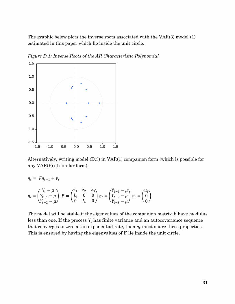
The graphic below plots the inverse roots associated with the VAR(3) model (1)

estimated in this paper which lie inside the unit circle.

Figure D.1: Inverse Roots of the AR Characteristic Polynomial

Alternatively, writing model (D.3) in VAR(1) companion form (which is possible for

any VAR(P) of similar form):

𝜂𝑡 = 𝐹𝜂𝑡−1 + 𝑣𝑡

𝜂𝑡 = (

Y𝑡 − 𝜇𝑌𝑡−1 − 𝜇𝑌𝑡−2 − 𝜇

) 𝐹 = (

z1 z2 z3𝐼4 0 00 𝐼4 0

) 𝜂𝑡 = (

Y𝑡−1 − 𝜇𝑌𝑡−2 − 𝜇𝑌𝑡−3 − 𝜇

) 𝑣𝑡 = (𝑢𝑡00)

The model will be stable if the eigenvalues of the companion matrix F have modulus

less than one. If the process Y𝑡 has finite variance and an autocovariance sequence

that converges to zero at an exponential rate, then 𝜂𝑡 must share these properties.

This is ensured by having the eigenvalues of F lie inside the unit circle.

-1.5

-1.0

-0.5

0.0

0.5

1.0

1.5

-1.5 -1.0 -0.5 0.0 0.5 1.0 1.5

Inverse Roots of AR Characteristic Polynomial

32

Appendix D: Cholesky Decomposition & the Identification Problem

Properties of the VAR(1) bivariate dynamic system generalizes to VAR(p) k-variable

systems and serves to illustrate the identification problem associated with the

VAR(3), or model (1), of this paper with implications for IRFs (see subsection 5.2):

(C.1) 𝑌𝑡 = 𝐻𝑌𝑡−1 + 𝑢𝑡 , where 𝑌𝑡 = (𝑌1, 𝑌2)′

Has properties:

𝐸(𝑢𝑡) = 0 and 𝐸(𝑢𝑡𝑢𝑡′) = Ω 𝑓𝑜𝑟 𝑠 = 𝑡0 𝑓𝑜𝑟 𝑠 ≠ 𝑡

The variance-covariance matrix Ω is assumed to be positive definite and the errors

are not serially uncorrelated but can be contemporaneously correlated (discussed

below). Model (C.1) with contemporaneous interactions (the structural VAR) is

represented:

(C.2) 𝐴𝑌𝑡 = 𝐵𝑌𝑡−1 + 𝜀𝑡

The model is structural since the special case of: 𝐴 = 𝐼 = (1 𝛼21𝛼12 1

) where 𝛼12 =

𝛼21 = 0 doesn’t hold. Written in reduced form:

𝑌𝑡 = 𝐴−1𝐵𝑌𝑡−1 + 𝐴

−1𝜀𝑡

Matrix 𝐴−1 appears in:

𝐻 = 𝐴−1𝐵 and 𝑢𝑡 = 𝐴−1𝜀𝑡

Assuming momentarily that 𝛼12 = 1.

(C.3) 𝐻𝑌𝑡−1 = (1 01 1

) (𝛽1 𝛽2𝛽3 𝛽4

) (𝑌1,𝑡−1𝑌2,𝑡−1

)=(𝛽1 𝛽2

𝛽1 + 𝛽3 𝛽2 + 𝛽4) (𝑌1,𝑡−1𝑌2,𝑡−1

)

From (C.3) it is evident that the lower triangular matrix 𝐴−1 causes the

contemporaneous values of the endogenous variables to enter the VAR model

recursively. More generally:

When 𝛼21 = 0 matrix A is lower triangular: 𝐴 = (1 0

−𝛼12 1) → 𝐴−1 = (

1 0𝛼12 1

)

33

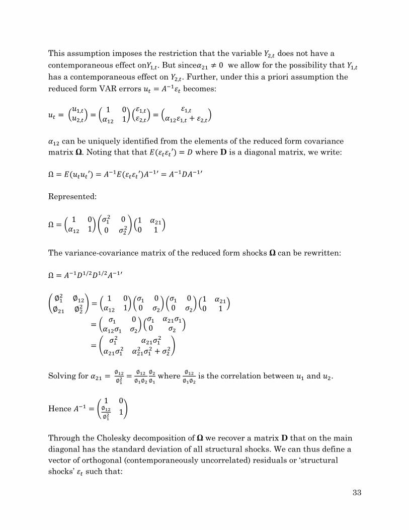
This assumption imposes the restriction that the variable 𝑌2,𝑡 does not have a

contemporaneous effect on𝑌1,𝑡. But since𝛼21 ≠ 0 we allow for the possibility that 𝑌1,𝑡

has a contemporaneous effect on 𝑌2,𝑡. Further, under this a priori assumption the

reduced form VAR errors 𝑢𝑡 = 𝐴−1𝜀𝑡 becomes:

𝑢𝑡 = (𝑢1,𝑡𝑢2,𝑡) = (

1 0𝛼12 1

) (𝜀1,𝑡𝜀2,𝑡) = (

𝜀1,𝑡𝛼12𝜀1,𝑡 + 𝜀2,𝑡

)

𝛼12 can be uniquely identified from the elements of the reduced form covariance

matrix Ω. Noting that that 𝐸(𝜀𝑡𝜀𝑡′) = 𝐷 where D is a diagonal matrix, we write:

Ω = 𝐸(𝑢𝑡𝑢𝑡′) = 𝐴−1𝐸(𝜀𝑡𝜀𝑡′)𝐴

−1′ = 𝐴−1𝐷𝐴−1′

Represented:

Ω = (1 0𝛼12 1

) (𝜎12 0

0 𝜎22) (

1 𝛼210 1

)

The variance-covariance matrix of the reduced form shocks Ω can be rewritten:

Ω = 𝐴−1𝐷1/2𝐷1/2𝐴−1′

(∅12 ∅12

∅21 ∅22 ) = (

1 0𝛼12 1

) (𝜎1 00 𝜎2

) (𝜎1 00 𝜎2

) (1 𝛼210 1

)

= (𝜎1 0𝛼12𝜎1 𝜎2

) (𝜎1 𝛼21𝜎10 𝜎2

)

= (𝜎12 𝛼21𝜎1

2

𝛼21𝜎12 𝛼21

2 𝜎12 + 𝜎2

2)

Solving for 𝛼21 = ∅12

∅12 =

∅12

∅1∅2

∅2

∅1 where

∅12

∅1∅2 is the correlation between 𝑢1 and 𝑢2.

Hence 𝐴−1 = (1 0∅12

∅12 1)

Through the Cholesky decomposition of Ω we recover a matrix D that on the main

diagonal has the standard deviation of all structural shocks. We can thus define a

vector of orthogonal (contemporaneously uncorrelated) residuals or ‘structural

shocks’ 𝜀𝑡 such that:

34

𝐸(𝜀𝑡𝜀𝑡′) = 𝐸(𝐴−1𝑢𝑡𝑢𝑡′𝐴

−1′) = 𝐴−1(𝐴𝐷𝐴′)𝐴−1′= 𝐷

The object of orthogonalizing the reduced form residuals therefore consists of

finding a transformation matrix A that expresses the structural residuals in terms

of linear combinations of the reduced form residuals. Thus the ordering of the

recursive structure is that imposed in the Cholesky decomposition. The uniqueness

of the Cholesky decomposition is with respect to the ordering within the vector 𝑌𝑡. In

the econometrics literature such a system is called a recursive model. Wold (1960)

has advocated these models where the researcher has to specify the instantaneous

causal ordering of the variables. This type of causality is therefore sometimes

referred to as Wold-causality or Wold causal ordering.

Furthermore, correlation of the error terms may indicate that a shock in one

variable is likely to be accompanied by a shock in another variable. In that case,

setting all other errors to zero may provide a misleading picture of the actual

dynamic relationships between the variables adversely affecting IRF results. This

can be overcome by structural identification through a recursive model such as

estimated in subsection 4.2. Giving the contemporaneous correlations a hierarchical

structure maintains Wold casual ordering.