Time Series Analysis and Forecasting CONTENTS STATISTICS IN PRACTICE: NEVADA OCCUPATIONAL HEALTH CLINIC 15.1 TIME SERIES PATTERNS Horizontal Pattern Trend Pattern Seasonal Pattern Trend and Seasonal Pattern Cyclical Pattern Using Excel’s Chart Tools to Construct a Time Series Plot Selecting a Forecasting Method 15.2 FORECAST ACCURACY 15.3 MOVING AVERAGES AND EXPONENTIAL SMOOTHING Moving Averages Using Excel’s Moving Average Tool Weighted Moving Averages Exponential Smoothing Using Excel’s Exponential Smoothing Tool 15.4 TREND PROJECTION Linear Trend Regression Using Excel’s Regression Tool to Compute a Linear Trend Equation Nonlinear Trend Regression Using Excel’s Regression Tool to Compute a Quadratic Trend Equation Using Excel’s Chart Tools for Trend Projection 15.5 SEASONALITY AND TREND Seasonality Without Trend Seasonality and Trend Models Based on Monthly Data 15.6 TIME SERIES DECOMPOSITION Calculating the Seasonal Indexes Deseasonalizing the Time Series Using the Deseasonalized Time Series to Identify Trend Seasonal Adjustments Models Based on Monthly Data Cyclical Component CHAPTER 15 © 2012 Cengage Learning. All Rights Reserved. May not be scanned, copied or duplicated, or posted to a publicly accessible website, in whole or in part.

Welcome message from author
This document is posted to help you gain knowledge. Please leave a comment to let me know what you think about it! Share it to your friends and learn new things together.
Transcript
Time Series Analysis and Forecasting
CONTENTS
STATISTICS IN PRACTICE:NEVADA OCCUPATIONAL HEALTH CLINIC
15.1 TIME SERIES PATTERNSHorizontal PatternTrend PatternSeasonal PatternTrend and Seasonal PatternCyclical PatternUsing Excel’s Chart Tools
to Construct a Time Series Plot
Selecting a Forecasting Method
15.2 FORECAST ACCURACY
15.3 MOVING AVERAGES AND EXPONENTIALSMOOTHINGMoving AveragesUsing Excel’s Moving
Average ToolWeighted Moving AveragesExponential SmoothingUsing Excel’s Exponential
Smoothing Tool
15.4 TREND PROJECTIONLinear Trend RegressionUsing Excel’s Regression Tool
to Compute a LinearTrend Equation
Nonlinear Trend RegressionUsing Excel’s Regression Tool
to Compute a QuadraticTrend Equation
Using Excel’s Chart Tools forTrend Projection
15.5 SEASONALITY AND TRENDSeasonality Without TrendSeasonality and TrendModels Based on Monthly Data
15.6 TIME SERIESDECOMPOSITIONCalculating the Seasonal IndexesDeseasonalizing the Time SeriesUsing the Deseasonalized Time
Series to Identify TrendSeasonal AdjustmentsModels Based on Monthly DataCyclical Component
CHAPTER 15
© 2012 Cengage Learning. All Rights Reserved. May not be scanned, copied or duplicated, or posted to a publicly accessible website, in whole or in part.

15-2 Chapter 15 Time Series Analysis and Forecasting
Nevada Occupational Health Clinic is a privately ownedmedical clinic in Sparks, Nevada. The clinic specializesin industrial medicine. Operating at the same site formore than 20 years, the clinic had been in a rapid growthphase. Monthly billings increased from $57,000 to morethan $300,000 in 26 months, when the main clinic build-ing burned to the ground.
The clinic’s insurance policy covered physical prop-erty and equipment as well as loss of income due to theinterruption of regular business operations. Settling theproperty insurance claim was a relatively straightforwardmatter of determining the value of the physical propertyand equipment lost during the fire. However, determiningthe value of the income lost during the seven months thatit took to rebuild the clinic was a complicated matterinvolving negotiations between the businessownersandtheinsurance company. No preestablished rules could helpcalculate “what would have happened” to the clinic’sbillings if the fire had not occurred. To estimate the lost in-come, the clinic used a forecasting method to project thegrowth in business that would have been realized duringthe seven-month lost-business period. The actual history ofbillings prior to the fire provided the basis for a forecastingmodel with linear trend and seasonal components as
discussed in this chapter. This forecasting model enabledthe clinic to establish an accurate estimate of the loss,which was eventually accepted by the insurance company.
NEVADA OCCUPATIONAL HEALTH CLINIC*SPARKS, NEVADA
STATISTICS in PRACTICE
*The authors are indebted to Bard Betz, Director of Operations, andCurtis Brauer, Executive Administrative Assistant, Nevada OccupationalHealth Clinic, for providing this Statistics in Practice.
The purpose of this chapter is to provide an introduction to time series analysis and fore-casting. Suppose we are asked to provide quarterly forecasts of sales for one of our com-pany’s products over the coming one-year period. Production schedules, raw materialpurchasing, inventory policies, and sales quotas will all be affected by the quarterly fore-casts we provide. Consequently, poor forecasts may result in poor planning and increasedcosts for the company. How should we go about providing the quarterly sales forecasts?Good judgment, intuition, and an awareness of the state of the economy may give us a roughidea or “feeling” of what is likely to happen in the future, but converting that feeling into anumber that can be used as next year’s sales forecast is difficult.
Forecasting methods can be classified as qualitative or quantitative. Qualitative meth-ods generally involve the use of expert judgment to develop forecasts. Such methods areappropriate when historical data on the variable being forecast are either not applicable orunavailable. Quantitative forecasting methods can be used when (1) past information aboutthe variable being forecast is available, (2) the information can be quantified, and (3) it isreasonable to assume that the pattern of the past will continue into the future. In such cases,
A physician checks a patient’s blood pressure at the Nevada Occupational Health Clinic.
©B
ob P
ardu
e–M
edic
al L
ifes
tyle
/Ala
my.
A forecast is simply aprediction of what willhappen in the future.Managers must learn toaccept that regardless ofthe technique used, theywill not be able to developperfect forecasts.
© 2012 Cengage Learning. All Rights Reserved. May not be scanned, copied or duplicated, or posted to a publicly accessible website, in whole or in part.

15.1 Time Series Patterns 15-3
a forecast can be developed using a time series method or a causal method. We will focusexclusively on quantitative forecasting methods in this chapter.
If the historical data are restricted to past values of the variable to be forecast, the fore-casting procedure is called a time series method and the historical data are referred to as atime series. The objective of time series analysis is to discover a pattern in the historicaldata or time series and then extrapolate the pattern into the future; the forecast is basedsolely on past values of the variable and/or on past forecast errors.
Causal forecasting methods are based on the assumption that the variable we are fore-casting has a cause-effect relationship with one or more other variables. In the discussionof regression analysis in Chapters 12 and 13, we showed how one or more independent vari-ables could be used to predict the value of a single dependent variable. Looking atregression analysis as a forecasting tool, we can view the time series value that we want toforecast as the dependent variable. Hence, if we can identify a good set of related indepen-dent, or explanatory, variables, we may be able to develop an estimated regression equationfor predicting or forecasting the time series. For instance, the sales for many products areinfluenced by advertising expenditures, so regression analysis may be used to develop anequation showing how sales and advertising expenditures are related. Once the advertisingbudget for the next period is determined, we could substitute this value into the equation todevelop a prediction or forecast of the sales volume for that period. Note that if a time se-ries method were used to develop the forecast, advertising expenditures would not be con-sidered; that is, a time series method would base the forecast solely on past sales.
By treating time as the independent variable and the time series variable as a dependentvariable, regression analysis can also be used as a time series method. To help differentiatethe application of regression analysis in these two cases, we use the terms cross-sectional regression and time series regression. Thus, time series regression refers to the use of regression analysis when the independent variable is time. Because our focus in this chapteris on time series methods, we leave the discussion of the application of regression analysisas a causal forecasting method to more advanced texts on forecasting.
Time Series PatternsA time series is a sequence of observations on a variable measured at successive points intime or over successive periods of time. The measurements may be taken every hour, day,week, month, or year, or at any other regular interval.1 The pattern of the data is an impor-tant factor in understanding how the time series has behaved in the past. If such behavior canbe expected to continue in the future, we can use the past pattern to guide us in selecting anappropriate forecasting method.
To identify the underlying pattern in the data, a useful first step is to construct a timeseries plot. A time series plot is a graphical presentation of the relationship between timeand the time series variable; time is on the horizontal axis and the time series values areshown on the vertical axis. Let us review some of the common types of data patterns thatcan be identified when examining a time series plot.
Horizontal PatternA horizontal pattern exists when the data fluctuate around a constant mean. To illustrate atime series with a horizontal pattern, consider the 12 weeks of data in Table 15.1. These data
15.1
fileWEBGasoline
1We limit our discussion to time series in which the values of the series are recorded at equal intervals. Cases in which theobservations are made at unequal intervals are beyond the scope of this text.
TABLE 15.1GASOLINE SALESTIME SERIES
Sales (1000sWeek of gallons)
1 172 213 194 235 186 167 208 189 22
10 2011 1512 22
© 2012 Cengage Learning. All Rights Reserved. May not be scanned, copied or duplicated, or posted to a publicly accessible website, in whole or in part.

show the number of gallons of gasoline sold by a gasoline distributor in Bennington, Vermont,over the past 12 weeks. The average value or mean for this time series is 19.25 or 19,250 gallons per week. Figure 15.1 shows a time series plot for these data. Note how the data fluctuate around the sample mean of 19,250 gallons. Although random variability is present,we would say that these data follow a horizontal pattern.
The term stationary time series2 is used to denote a time series whose statistical prop-erties are independent of time. In particular this means that
1. The process generating the data has a constant mean.2. The variability of the time series is constant over time.
A time series plot for a stationary time series will always exhibit a horizontal pattern. Butsimply observing a horizontal pattern is not sufficient evidence to conclude that the timeseries is stationary. More advanced texts on forecasting discuss procedures for determiningif a time series is stationary and provide methods for transforming a time series that is notstationary into a stationary series.
Changes in business conditions can often result in a time series that has a horizontalpattern shifting to a new level. For instance, suppose the gasoline distributor signs a con-tract with the Vermont State Police to provide gasoline for state police cars located insouthern Vermont. With this new contract, the distributor expects to see a major increasein weekly sales starting in week 13. Table 15.2 shows the number of gallons of gasoline soldfor the original time series and for the 10 weeks after signing the new contract. Figure 15.2 shows the corresponding time series plot. Note the increased level of the timeseries beginning in week 13. This change in the level of the time series makes it more dif-ficult to choose an appropriate forecasting method. Selecting a forecasting method thatadapts well to changes in the level of a time series is an important consideration in manypractical applications.
15-4 Chapter 15 Time Series Analysis and Forecasting
Sale
s (1
000s
of
gallo
ns)
0
20
15
10
5
04 7 9
Week
25
1 2 3 65 8 10 1211
FIGURE 15.1 GASOLINE SALES TIME SERIES PLOT
2For a formal definition of stationary, see G. E. P., Box, G. M. Jenkins, and G. C. Reinsell, Time Series Analysis: Forecastingand Control, 3rd ed. Englewood Cliffs, NJ: Prentice Hall, 1994, p. 23.
TABLE 15.2GASOLINE SALESTIME SERIES AFTEROBTAINING THECONTRACT WITHTHE VERMONT STATE POLICE
Sales (1000sWeek of gallons)
1 172 213 194 235 186 167 208 189 22
10 2011 1512 2213 3114 3415 3116 3317 2818 3219 3020 2921 3422 33
fileWEBGasolineRevised
© 2012 Cengage Learning. All Rights Reserved. May not be scanned, copied or duplicated, or posted to a publicly accessible website, in whole or in part.

15.1 Time Series Patterns 15-5
Trend PatternAlthough time series data generally exhibit random fluctuations, a time series may also showgradual shifts or movements to relatively higher or lower values over a longer period of time.If a time series plot exhibits this type of behavior, we say that a trend pattern exists. A trendis usually the result of long-term factors such as population increases or decreases, changingdemographic characteristics of the population, technology, and/or consumer preferences.
To illustrate a time series with a trend pattern, consider the time series of bicycle salesfor a particular manufacturer over the past 10 years, as shown in Table 15.3 and Figure 15.3.Note that 21,600 bicycles were sold in year one, 22,900 were sold in year two, and so on.In year 10, the most recent year, 31,400 bicycles were sold. Visual inspection of the timeseries plot shows some up and down movement over the past 10 years, but the time seriesalso seems to have a systematically increasing or upward trend.
The trend for the bicycle sales time series appears to be linear and increasing over time,but sometimes a trend can be described better by other types of patterns. For instance, thedata in Table 15.4 and the corresponding time series plot in Figure 15.4 show the sales fora cholesterol drug since the company won FDA approval for it 10 years ago. The time series increases in a nonlinear fashion; that is, the rate of change of revenue does not increaseby a constant amount from one year to the next. In fact, the revenue appears to be growingin an exponential fashion. Exponential relationships such as this are appropriate when thepercentage change from one period to the next is relatively constant.
Seasonal PatternThe trend of a time series can be identified by analyzing multiyear movements in historicaldata. Seasonal patterns are recognized by seeing the same repeating patterns over succes-sive periods of time. For example, a manufacturer of swimming pools expects low sales
Sale
s (1
000s
of
gallo
ns)
0
15
20
25
30
35
10
5
04 7 9
Week
40
1 2 3 65 8 10 12 13 14 15 16 17 18 19 20 21 22 23 2411
FIGURE 15.2 GASOLINE SALES TIME SERIES PLOT AFTER OBTAINING THE CONTRACT WITH THE VERMONT STATE POLICE
TABLE 15.3BICYCLE SALESTIME SERIES
Year Sales (1000s)1 21.62 22.93 25.54 21.95 23.96 27.57 31.58 29.79 28.6
10 31.4
fileWEBBicycle
© 2012 Cengage Learning. All Rights Reserved. May not be scanned, copied or duplicated, or posted to a publicly accessible website, in whole or in part.

activity in the fall and winter months, with peak sales in the spring and summer months.Manufacturers of snow removal equipment and heavy clothing, however, expect just theopposite yearly pattern. Not surprisingly, the pattern for a time series plot that exhibits a re-peating pattern over a one-year period due to seasonal influences is called a seasonal pat-tern. While we generally think of seasonal movement in a time series as occurring withinone year, time series data can also exhibit seasonal patterns of less than one year in dura-tion. For example, daily traffic volume shows within-the-day “seasonal” behavior, withpeak levels occurring during rush hours, moderate flow during the rest of the day and earlyevening, and light flow from midnight to early morning.
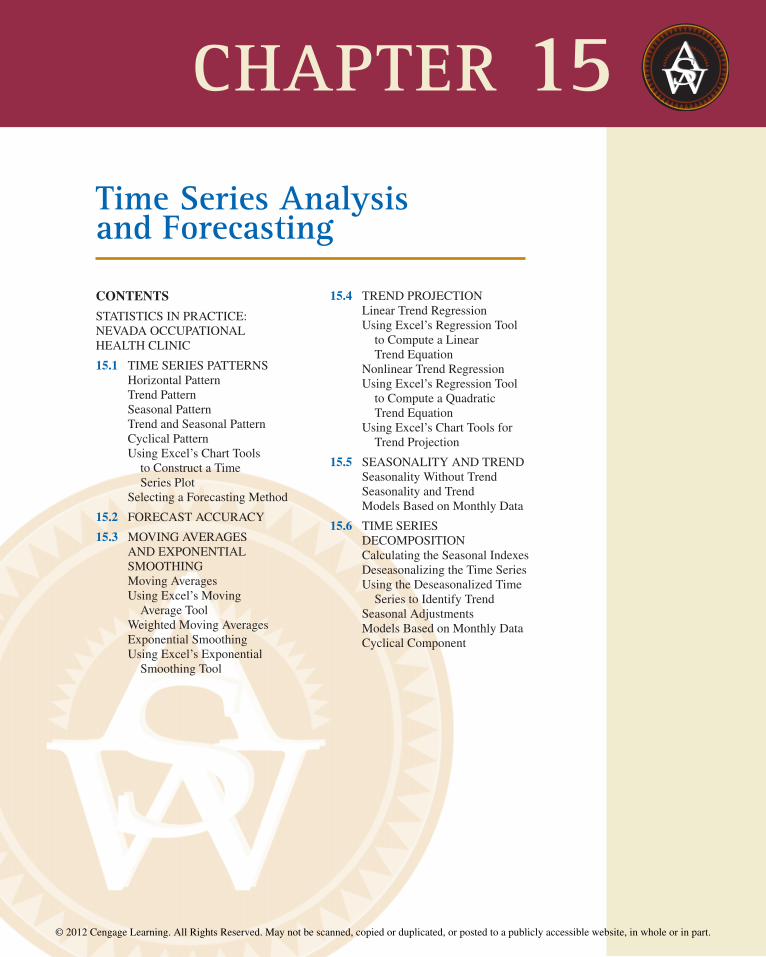
As an example of a seasonal pattern, consider the number of umbrellas sold at aclothing store over the past five years. Table 15.5 shows the time series and Figure 15.5shows the corresponding time series plot. The time series plot does not indicate anylong-term trend in sales. In fact, unless you look carefully at the data, you might con-clude that the data follow a horizontal pattern. But closer inspection of the time seriesplot reveals a regular pattern in the data. That is, the first and third quarters have mod-erate sales, the second quarter has the highest sales, and the fourth quarter tends to havethe lowest sales volume. Thus, we would conclude that a quarterly seasonal pattern ispresent.
Trend and Seasonal PatternSome time series include a combination of a trend and seasonal pattern. For instance, thedata in Table 15.6 and the corresponding time series plot in Figure 15.6 show television setsales for a particular manufacturer over the past four years. Clearly, an increasing trend ispresent. But Figure 15.6 also indicates that sales are lowest in the second quarter of eachyear and increase in quarters 3 and 4. Thus, we conclude that a seasonal pattern also existsfor television set sales. In such cases we need to use a forecasting method that has the capability to deal with both trend and seasonality.
15-6 Chapter 15 Time Series Analysis and Forecasting
Sale
s (1
000s
)
0
22
24
26
28
30
32
204 7 9
Year
34
1 2 3 65 8 10 1211
FIGURE 15.3 BICYCLE SALES TIME SERIES PLOT
TABLE 15.4CHOLESTEROLREVENUETIME SERIES ($MILLIONS)
Year Revenue1 23.12 21.33 27.44 34.65 33.86 43.27 59.58 64.49 74.2
10 99.3
fileWEBCholesterol
© 2012 Cengage Learning. All Rights Reserved. May not be scanned, copied or duplicated, or posted to a publicly accessible website, in whole or in part.

15.1 Time Series Patterns 15-7
Cyclical PatternA cyclical pattern exists if the time series plot shows an alternating sequence of pointsbelow and above the trend line lasting more than one year. Many economic time seriesexhibit cyclical behavior with regular runs of observations below and above the trend line.
Rev
enue
0
20
40
60
80
100
04 7 9
Year
120
1 2 3 65 8 10
FIGURE 15.4 CHOLESTEROL REVENUE TIMES SERIES PLOT ($MILLIONS)
Year Quarter Sales1 1 125
2 1533 1064 88
2 1 1182 1613 1334 102
3 1 1382 1443 1134 80
4 1 1092 1373 1254 109
5 1 1302 1653 1284 96
TABLE 15.5 UMBRELLA SALES TIME SERIES
fileWEBUmbrella
© 2012 Cengage Learning. All Rights Reserved. May not be scanned, copied or duplicated, or posted to a publicly accessible website, in whole or in part.
Often, the cyclical component of a time series is due to multiyear business cycles. For ex-ample, periods of moderate inflation followed by periods of rapid inflation can lead to timeseries that alternate below and above a generally increasing trend line (e.g., a time series forhousing costs). Business cycles are extremely difficult, if not impossible, to forecast. As a result, cyclical effects are often combined with long-term trend effects and referred to astrend-cycle effects. In this chapter we do not deal with cyclical effects that may be presentin the time series.
15-8 Chapter 15 Time Series Analysis and Forecasting
Sale
s
60
80
100
120
160
140
40
20
0
180
1 2 3 4 1 2 3 4 1 2 3 4 1 2 3 4
Year 1 Year 2 Year 3 Year 4
1 2 3 4
Year 5
Year/Quarter
FIGURE 15.5 UMBRELLA SALES TIME SERIES PLOT
Year Quarter Sales (1000s)1 1 4.8
2 4.13 6.04 6.5
2 1 5.82 5.23 6.84 7.4
3 1 6.02 5.63 7.54 7.8
4 1 6.32 5.93 8.04 8.4
TABLE 15.6 QUARTERLY TELEVISION SET SALES TIME SERIES
fileWEBTVSales
© 2012 Cengage Learning. All Rights Reserved. May not be scanned, copied or duplicated, or posted to a publicly accessible website, in whole or in part.

15.1 Time Series Patterns 15-9
Using Excel’s Chart Tools to Construct a Time Series PlotWe can use Excel’s chart tools to construct a time series plot. The following steps show howto construct a time series plot for the gasoline time series in Table 15.1. Refer to Figure 15.7as we describe the tasks involved.
Step 1. Select cells A2:B13Step 2. Click the Insert tab on the Excel RibbonStep 3. In the Charts group, click ScatterStep 4. When the list of scatter diagram subtypes appears,
Click Scatter with Straight Lines and Markers (the second chart in column 2)
Step 5. In the Chart Layouts group, click Layout 1Step 6. Select the Chart Title and replace it with Time Series Plot for the Gasoline
Sales Time SeriesStep 7. Select the Horizontal (Value) Axis Title and replace it with WeekStep 8. Select the Vertical (Value) Axis Title and replace it with Sales (1000s of
gallons)Step 9. Right-click the Series 1 Legend Entry and click Delete
The worksheet displayed in Figure 15.7 shows the time series plot produced by Excel.
Selecting a Forecasting MethodThe underlying pattern in the time series is an important factor in selecting a forecast-ing method. Thus, a time series plot should be one of the first things developed whentrying to determine what forecasting method to use. If we see a horizontal pattern, thenwe need to select a method appropriate for this type of pattern. Similarly, if we observe
Qua
rter
ly T
elev
isio
n Se
t Sa
les
(100
0s)
9.0
1
3.0
4.0
5.0
6.0
7.0
8.0
0.0
1.0
2.0
2 3 4 1 2 3 4 1 2 3 4 1 2 3 4
Year 1 Year 2 Year 3 Year 4
Year/Quarter
FIGURE 15.6 QUARTERLY TELEVISION SET SALES TIME SERIES PLOT
A time series plot is simplya scatter diagram with linesconnecting the points. Weshowed how construct ascatter diagram in Sections2.4 and 12.2.
© 2012 Cengage Learning. All Rights Reserved. May not be scanned, copied or duplicated, or posted to a publicly accessible website, in whole or in part.

a trend in the data, then we need to use a forecasting method that has the capability tohandle trend effectively. The next two sections illustrate methods that can be used in sit-uations where the underlying pattern is horizontal; in other words, no trend or seasonaleffects are present. We then consider methods appropriate when trend and/or seasonal-ity are present in the data.
Forecast AccuracyIn this section we begin by developing forecasts for the gasoline time series shown inTable 15.1 using the simplest of all the forecasting methods: an approach that uses the mostrecent week’s sales volume as the forecast for the next week. For instance, the distributorsold 17 thousand gallons of gasoline in week 1; this value is used as the forecast for week 2.Next, we use 21, the actual value of sales in week 2, as the forecast for week 3, and so on.The forecasts obtained for the historical data using this method are shown in Table 15.7 inthe column labeled Forecast. Because of its simplicity, this method is often referred to as anaive forecasting method.
How accurate are the forecasts obtained using this naive forecasting method? To answer this question we will introduce several measures of forecast accuracy. These measuresare used to determine how well a particular forecasting method is able to reproduce the timeseries data that are already available. By selecting the method that has the best accuracy forthe data already known, we hope to increase the likelihood that we will obtain better fore-casts for future time periods.
The key concept associated with measuring forecast accuracy is forecast error,defined as
Forecast Error � ActualValue � Forecast
15.2
15-10 Chapter 15 Time Series Analysis and Forecasting
FIGURE 15.7 TIME SERIES PLOT FOR THE GASOLINE SALES TIME SERIES USING EXCEL’S CHART TOOLS
© 2012 Cengage Learning. All Rights Reserved. May not be scanned, copied or duplicated, or posted to a publicly accessible website, in whole or in part.

15.2 Forecast Accuracy 15-11
For instance, because the distributor actually sold 21 thousand gallons of gasoline in week 2and the forecast, using the sales volume in week 1, was 17 thousand gallons, the forecasterror in week 2 is
The fact that the forecast error is positive indicates that in week 2 the forecasting methodunderestimated the actual value of sales. Next, we use 21, the actual value of sales in week2, as the forecast for week 3. Since the actual value of sales in week 3 is 19, the forecast error for week 3 is 19 � 21 � �2. In this case, the negative forecast error indicates that inweek 3 the forecast overestimated the actual value. Thus, the forecast error may be positiveor negative, depending on whether the forecast is too low or too high. A complete summaryof the forecast errors for this naive forecasting method is shown in Table 15.7 in the columnlabeled Forecast Error.
A simple measure of forecast accuracy is the mean or average of the forecast errors.Table 15.7 shows that the sum of the forecast errors for the gasoline sales time series is 5;thus, the mean or average forecast error is 5/11 � .45. Note that although the gasoline timeseries consists of 12 values, to compute the mean error we divided the sum of the forecasterrors by 11 because there are only 11 forecast errors. Because the mean forecast error ispositive, the method is underforecasting; in other words, the observed values tend to begreater than the forecasted values. Because positive and negative forecast errors tend to off-set one another, the mean error is likely to be small; thus, the mean error is not a very use-ful measure of forecast accuracy.
The mean absolute error, denoted MAE, is a measure of forecast accuracy thatavoids the problem of positive and negative forecast errors offsetting one another. As youmight expect given its name, MAE is the average of the absolute values of the forecasterrors. Table 15.7 shows that the sum of the absolute values of the forecast errors is 41;thus,
MAE � average of the absolute value of forecast errors �41
11� 3.73
Forecast Error in week 2 � 21 � 17 � 4
Time Absolute Value Squared Absolute ValueSeries Forecast of Forecast Forecast Percentage of Percentage
Week Value Forecast Error Error Error Error Error1 172 21 17 4 4 16 19.05 19.053 19 21 �2 2 4 �10.53 10.534 23 19 4 4 16 17.39 17.395 18 23 �5 5 25 �27.78 27.786 16 18 �2 2 4 �12.50 12.507 20 16 4 4 16 20.00 20.008 18 20 �2 2 4 �11.11 11.119 22 18 4 4 16 18.18 18.18
10 20 22 �2 2 4 �10.00 10.0011 15 20 �5 5 25 �33.33 33.3312 22 15 7 7 49 31.82 31.82
Totals 5 41 179 1.19 211.69
TABLE 15.7 COMPUTING FORECASTS AND MEASURES OF FORECAST ACCURACY USING THEMOST RECENT VALUE AS THE FORECAST FOR THE NEXT PERIOD
In regression analysis, aresidual is defined as thedifference between theobserved value of thedependent variable and theestimated value. Theforecast errors areanalogous to the residualsin regression analysis.
© 2012 Cengage Learning. All Rights Reserved. May not be scanned, copied or duplicated, or posted to a publicly accessible website, in whole or in part.

Another measure that avoids the problem of positive and negative forecast errors off-setting each other is obtained by computing the average of the squared forecast errors. Thismeasure of forecast accuracy, referred to as the mean squared error, is denoted MSE.From Table 15.7, the sum of the squared errors is 179; hence,
The size of MAE and MSE depends upon the scale of the data. As a result, it is dif-ficult to make comparisons for different time intervals, such as comparing a method offorecasting monthly gasoline sales to a method of forecasting weekly sales, or to makecomparisons across different time series. To make comparisons like these we need towork with relative or percentage error measures. The mean absolute percentage error,denoted MAPE, is such a measure. To compute MAPE we must first compute the per-centage error for each forecast. For example, the percentage error corresponding to theforecast of 17 in week 2 is computed by dividing the forecast error in week 2 by the ac-tual value in week 2 and multiplying the result by 100. For week 2 the percentage erroris computed as follows:
Thus, the forecast error for week 2 is 19.05% of the observed value in week 2. A completesummary of the percentage errors is shown in Table 15.7 in the column labeled PercentageError. In the next column, we show the absolute value of the percentage error.
Table 15.7 shows that the sum of the absolute values of the percentage errors is211.69; thus,
Summarizing, using the naive (most recent observation) forecasting method, we obtainedthe following measures of forecast accuracy:
MAE � 3.73
MSE � 16.27
MAPE � 19.24%
These measures of forecast accuracy simply measure how well the forecasting methodis able to forecast historical values of the time series. Now, suppose we want to forecastsales for a future time period, such as week 13. In this case the forecast for week 13 is 22,the actual value of the time series in week 12. Is this an accurate estimate of sales forweek 13? Unfortunately, there is no way to address the issue of accuracy associated withforecasts for future time periods. But if we select a forecasting method that works well forthe historical data, and we think that the historical pattern will continue into the future, weshould obtain results that will ultimately be shown to be good.
Before closing this section, let’s consider another method for forecasting the gasolinesales time series in Table 15.1. Suppose we use the average of all the historical data avail-able as the forecast for the next period. We begin by developing a forecast for week 2. Sincethere is only one historical value available prior to week 2, the forecast for week 2 is just
MAPE � average of the absolute value of percentage forecast errors �211.69
11� 19.24%
Percentage error for week 2 �4
21(100) � 19.05%
MSE � average of the sum of squared forecast errors �179
11� 16.27
15-12 Chapter 15 Time Series Analysis and Forecasting
In regression analysis, themean square error (MSE) isthe residual sum of squaresdivided by its degrees offreedom. In forecasting,MSE is the average of thesum of squared forecasterrors.
An Excel worksheet canfacilitate making thecalculations in Table 15.7.
© 2012 Cengage Learning. All Rights Reserved. May not be scanned, copied or duplicated, or posted to a publicly accessible website, in whole or in part.

15.2 Forecast Accuracy 15-13
the time series value in week 1; thus, the forecast for week 2 is 17 thousand gallons of gaso-line. To compute the forecast for week 3, we take the average of the sales values in weeks1 and 2. Thus,
Similarly, the forecast for week 4 is
The forecasts obtained using this method for the gasoline time series are shown in Table 15.8 in the column labeled Forecast. Using the results shown in Table 15.8, we obtained the following values of MAE, MSE, and MAPE:
We can now compare the accuracy of the two forecasting methods we have consid-ered in this section by comparing the values of MAE, MSE, and MAPE for each method.
MAPE �141.34
11� 12.85%
MSE �89.07
11� 8.10
MAE �26.81
11� 2.44
Forecast for week 4 �17 � 21 � 19
3� 19
Forecast for week 3 �17 � 21
2� 19
Time Absolute Value Squared Absolute ValueSeries Forecast of Forecast Forecast Percentage of Percentage
Week Value Forecast Error Error Error Error Error1 172 21 17.00 4.00 4.00 16.00 19.05 19.053 19 19.00 0.00 0.00 0.00 0.00 0.004 23 19.00 4.00 4.00 16.00 17.39 17.395 18 20.00 �2.00 2.00 4.00 �11.11 11.116 16 19.60 �3.60 3.60 12.96 �22.50 22.507 20 19.00 1.00 1.00 1.00 5.00 5.008 18 19.14 �1.14 1.14 1.31 �6.35 6.359 22 19.00 3.00 3.00 9.00 13.64 13.64
10 20 19.33 0.67 0.67 0.44 3.33 3.3311 15 19.40 �4.40 4.40 19.36 �29.33 29.3312 22 19.00 3.00 3.00 9.00 13.64 13.64
Totals 4.53 26.81 89.07 2.76 141.34
TABLE 15.8 COMPUTING FORECASTS AND MEASURES OF FORECAST ACCURACY USING THEAVERAGE OF ALL THE HISTORICAL DATA AS THE FORECAST FOR THE NEXT PERIOD
Naive Method Average of Past Values
MAE 3.73 2.44MSE 16.27 8.10MAPE 19.24% 12.85%
© 2012 Cengage Learning. All Rights Reserved. May not be scanned, copied or duplicated, or posted to a publicly accessible website, in whole or in part.

For every measure, the average of past values provides more accurate forecasts thanusing the most recent observation as the forecast for the next period. In general, if theunderlying time series is stationary, the average of all the historical data will always pro-vide the best results.
But suppose that the underlying time series is not stationary. In Section 15.1 we men-tioned that changes in business conditions can often result in a time series that has a hor-izontal pattern shifting to a new level. We discussed a situation in which the gasolinedistributor signed a contract with the Vermont State Police to provide gasoline for statepolice cars located in southern Vermont. Table 15.2 shows the number of gallons of gaso-line sold for the original time series and the 10 weeks after signing the new contract, andFigure 15.2 shows the corresponding time series plot. Note the change in level in week 13for the resulting time series. When a shift to a new level like this occurs, it takes a longtime for the forecasting method that uses the average of all the historical data to adjust tothe new level of the time series. But, in this case, the simple naive method adjusts veryrapidly to the change in level because it uses the most recent observation available as theforecast.
Measures of forecast accuracy are important factors in comparing different forecastingmethods, but we have to be careful not to rely upon them too heavily. Good judgment andknowledge about business conditions that might affect the forecast also have to be carefullyconsidered when selecting a method. And historical forecast accuracy is not the only con-sideration, especially if the time series is likely to change in the future.
In the next section we will introduce more sophisticated methods for developingforecasts for a time series that exhibits a horizontal pattern. Using the measures of forecastaccuracy developed here, we will be able to determine if such methods provide moreaccurate forecasts than we obtained using the simple approaches illustrated in this section.The methods that we will introduce also have the advantage of adapting well in situationswhere the time series changes to a new level. The ability of a forecasting method to adaptquickly to changes in level is an important consideration, especially in short-termforecasting situations.
Exercises
Methods1. Consider the following time series data.
Week 1 2 3 4 5 6
Value 18 13 16 11 17 14
Using the naive method (most recent value) as the forecast for the next week, compute thefollowing measures of forecast accuracy.a. Mean absolute errorb. Mean squared errorc. Mean absolute percentage errord. What is the forecast for week 7?
2. Refer to the time series data in exercise 1. Using the average of all the historical data as aforecast for the next period, compute the following measures of forecast accuracy.a. Mean absolute errorb. Mean squared error
15-14 Chapter 15 Time Series Analysis and Forecasting
testSELF
testSELF
© 2012 Cengage Learning. All Rights Reserved. May not be scanned, copied or duplicated, or posted to a publicly accessible website, in whole or in part.

15.3 Moving Averages and Exponential Smoothing 15-15
c. Mean absolute percentage errord. What is the forecast for week 7?
3. Exercises 1 and 2 used different forecasting methods. Which method appears to providethe more accurate forecasts for the historical data? Explain.
4. Consider the following time series data.
Month 1 2 3 4 5 6 7
Value 24 13 20 12 19 23 15
a. Compute MSE using the most recent value as the forecast for the next period. What isthe forecast for month 8?
b. Compute MSE using the average of all the data available as the forecast for the nextperiod. What is the forecast for month 8?
c. Which method appears to provide the better forecast?
Moving Averages and ExponentialSmoothingIn this section we discuss three forecasting methods that are appropriate for a time serieswith a horizontal pattern: moving averages, weighted moving averages, and exponentialsmoothing. These methods also adapt well to changes in the level of a horizontal patternsuch as we saw with the extended gasoline sales time series (Table 15.2 and Figure 15.2).However, without modification they are not appropriate when significant trend, cyclical, orseasonal effects are present. Because the objective of each of these methods is to “smoothout” the random fluctuations in the time series, they are referred to as smoothing methods.These methods are easy to use and generally provide a high level of accuracy for short-rangeforecasts, such as a forecast for the next time period.
Moving AveragesThe moving averages method uses the average of the most recent k data values in the timeseries as the forecast for the next period. Mathematically, a moving average forecast of order k is as follows:
15.3
testSELF
MOVING AVERAGE FORECAST OF ORDER k
(15.1)
where
Ft�1 � forecast of the times series for period t � 1
Yt � actual value of the time series in period t
Ft�1 �� (most recent k data values)
k�
Yt � Yt�1 � . . . � Yt�k�1
k
© 2012 Cengage Learning. All Rights Reserved. May not be scanned, copied or duplicated, or posted to a publicly accessible website, in whole or in part.

The term moving is used because every time a new observation becomes available for the time series, it replaces the oldest observation in the equation and a new average is com-puted. As a result, the average will change, or move, as new observations become available.
To illustrate the moving averages method, let us return to the gasoline sales data inTable 15.1 and Figure 15.1. The time series plot in Figure 15.1 indicates that the gasolinesales time series has a horizontal pattern. Thus, the smoothing methods of this section areapplicable.
To use moving averages to forecast a time series, we must first select the order, or number of time series values, to be included in the moving average. If only the most recentvalues of the time series are considered relevant, a small value of k is preferred. If more pastvalues are considered relevant, then a larger value of k is better. As mentioned earlier, a timeseries with a horizontal pattern can shift to a new level over time. A moving average willadapt to the new level of the series and resume providing good forecasts in k periods. Thus,a smaller value of k will track shifts in a time series more quickly. But larger values of k willbe more effective in smoothing out the random fluctuations over time. So managerial judg-ment based on an understanding of the behavior of a time series is helpful in choosing agood value for k.
To illustrate how moving averages can be used to forecast gasoline sales, we will use athree-week moving average (k � 3). We begin by computing the forecast of sales in week4 using the average of the time series values in weeks 1–3.
1–3
Thus, the moving average forecast of sales in week 4 is 19 or 19,000 gallons of gasoline.Because the actual value observed in week 4 is 23, the forecast error in week 4 is 23 � 19 � 4.
Next, we compute the forecast of sales in week 5 by averaging the time series values inweeks 2–4.
2–4
Hence, the forecast of sales in week 5 is 21 and the error associated with this forecast is18 � 21 � �3. A complete summary of the three-week moving average forecasts forthe gasoline sales time series is provided in Table 15.9. Figure 15.8 shows the originaltime series plot and the three-week moving average forecasts. Note how the graph of themoving average forecasts has tended to smooth out the random fluctuations in the timeseries.
To forecast sales in week 13, the next time period in the future, we simply compute theaverage of the time series values in weeks 10, 11, and 12.
10–12
Thus, the forecast for week 13 is 19 or 19,000 gallons of gasoline.
Using Excel’s Moving Average ToolThe following steps describe how to use Excel’s Moving Average tool to develop the three-week moving average forecasts for the gasoline sales time series in Table 15.1. Refer toFigure 15.9 as we describe the tasks involved.
Step 1. Click the Data tab on the RibbonStep 2. In the Analysis group, click Data Analysis
�20 � 15 � 22
3� 19F13 � average of weeks
�21 � 19 � 23
3� 21F5 � average of weeks
�17 � 21 � 19
3� 19F4 � average of weeks
15-16 Chapter 15 Time Series Analysis and Forecasting
© 2012 Cengage Learning. All Rights Reserved. May not be scanned, copied or duplicated, or posted to a publicly accessible website, in whole or in part.

15.3 Moving Averages and Exponential Smoothing 15-17
Step 3. Choose Moving Average from the list of Analysis ToolsStep 4. When the Moving Average dialog box appears,
Enter B2:B13 in the Input Range boxEnter 3 in the Interval boxEnter C3 in the Output Range boxSelect Chart OutputClick OK
Time Absolute Value Squared Absolute ValueSeries Forecast of Forecast Forecast Percentage of Percentage
Week Value Forecast Error Error Error Error Error1 172 213 194 23 19 4 4 16 17.39 17.395 18 21 �3 3 9 �16.67 16.676 16 20 �4 4 16 �25.00 25.007 20 19 1 1 1 5.00 5.008 18 18 0 0 0 0.00 0.009 22 18 4 4 16 18.18 18.18
10 20 20 0 0 0 0.00 0.0011 15 20 �5 5 25 �33.33 33.3312 22 19 3 3 9 13.64 13.64
Totals 0 24 92 �20.79 129.21
TABLE 15.9 SUMMARY OF THREE-WEEK MOVING AVERAGE CALCULATIONS
Sale
s (1
000s
of
gallo
ns)
0
20
15
10
5
04 7 9
Week
25
1 2 3 65 8 10 1211
Three-week movingaverage forecasts
FIGURE 15.8 GASOLINE SALES TIME SERIES PLOT AND THREE-WEEK MOVINGAVERAGE FORECASTS
© 2012 Cengage Learning. All Rights Reserved. May not be scanned, copied or duplicated, or posted to a publicly accessible website, in whole or in part.

The three-week moving average forecasts appear in column C of the worksheet. Forecasts forperiods of other length can be computed easily by entering a different value in the interval box.
Forecast accuracy In Section 15.2 we discussed three measures of forecast accuracy:MAE, MSE, and MAPE. Using the three-week moving average calculations in Table 15.9,the values for these three measures of forecast accuracy are
In Section 15.2 we also showed that using the most recent observation as the forecast for the next week (a moving average of order k � 1) resulted in values of MAE � 3.73,MSE � 16.27, and MAPE � 19.24%. Thus, in each case the three-week moving averageapproach provided more accurate forecasts than simply using the most recent observationas the forecast.
To determine if a moving average with a different order k can provide more accurateforecasts, we recommend using trial and error to determine the value of k that minimizesMSE. For the gasoline sales time series, it can be shown that the minimum value of MSEcorresponds to a moving average of order k � 6 with MSE � 6.79. If we are willing to assume that the order of the moving average that is best for the historical data will also be
MAPE �129.21
9� 14.36%
MSE �92
9� 10.22
MAE �24
9� 2.67
15-18 Chapter 15 Time Series Analysis and Forecasting
FIGURE 15.9 THREE-WEEK MOVING AVERAGE FORECASTS FOR THE GASOLINE TIME SERIES USING EXCEL’S MOVING AVERAGE TOOL
In situations where youneed to compareforecasting methods fordifferent time periods, suchas comparing a forecast ofweekly sales to a forecast ofmonthly sales, relativemeasures such as MAPEare preferred.
© 2012 Cengage Learning. All Rights Reserved. May not be scanned, copied or duplicated, or posted to a publicly accessible website, in whole or in part.

15.3 Moving Averages and Exponential Smoothing 15-19
best for future values of the time series, the most accurate moving average forecasts of gaso-line sales can be obtained using a moving average of order k � 6.
Weighted Moving AveragesIn the moving averages method, each observation in the moving average calculation receives the same weight. One variation, known as weighted moving averages, involvesselecting a different weight for each data value and then computing a weighted average ofthe most recent k values as the forecast. In most cases, the most recent observation receivesthe most weight, and the weight decreases for older data values. Let us use the gasoline salestime series to illustrate the computation of a weighted three-week moving average. We assign a weight of 3/6 to the most recent observation, a weight of 2/6 to the second most recent observation, and a weight of 1/6 to the third most recent observation. Using thisweighted average, our forecast for week 4 is computed as follows:
Note that for the weighted moving average method the sum of the weights is equal to 1.
Forecast accuracy To use the weighted moving averages method, we must first select thenumber of data values to be included in the weighted moving average and then chooseweights for each of the data values. In general, if we believe that the recent past is a betterpredictor of the future than the distant past, larger weights should be given to the more recent observations. However, when the time series is highly variable, selecting approxi-mately equal weights for the data values may be best. The only requirement in selecting theweights is that their sum must equal 1. To determine whether one particular combination ofnumber of data values and weights provides a more accurate forecast than another combi-nation, we recommend using MSE as the measure of forecast accuracy. That is, if we as-sume that the combination that is best for the past will also be best for the future, we woulduse the combination of number of data values and weights that minimizes MSE for the his-torical time series to forecast the next value in the time series.
Exponential SmoothingExponential smoothing also uses a weighted average of past time series values as a fore-cast; it is a special case of the weighted moving averages method in which we select onlyone weight—the weight for the most recent observation. The weights for the other data val-ues are computed automatically and become smaller as the observations move farther intothe past. The exponential smoothing equation follows.
Forecast for week 4 � 1�6(17) � 2�6(21) � 3�6(19) � 19.33
A moving average forecastof order k � 3 is just aspecial case of the weightedmoving averages method inwhich each weight is equalto 1/3.
There are a number ofexponential smoothingprocedures. The methodpresented here is oftenreferred to as singleexponential smoothing. Inthe next section we showhow an exponentialsmoothing method that usestwo smoothing constantscan be used to forecast atime series with a lineartrend.
EXPONENTIAL SMOOTHING FORECAST
(15.2)
where
Ft�1 �
Yt �
Ft �
α �
forecast of the time series for period t � 1
actual value of the time series in period t
forecast of the time series for period t
smoothing constant (0 � α � 1)
Ft�1 � αYt � (1 � α)Ft
© 2012 Cengage Learning. All Rights Reserved. May not be scanned, copied or duplicated, or posted to a publicly accessible website, in whole or in part.

Equation (15.2) shows that the forecast for period t � 1 is a weighted average of theactual value in period t and the forecast for period t. The weight given to the actual value inperiod t is the smoothing constant α and the weight given to the forecast in period t is 1 – α.It turns out that the exponential smoothing forecast for any period is actually a weighted average of all the previous actual values of the time series. Let us illustrate by working witha time series involving only three periods of data: Y1, Y2, and Y3.
To initiate the calculations, we let F1 equal the actual value of the time series in period 1;that is, F1 � Y1. Hence, the forecast for period 2 is
We see that the exponential smoothing forecast for period 2 is equal to the actual value ofthe time series in period 1.
The forecast for period 3 is
Finally, substituting this expression for F3 in the expression for F4, we obtain
We now see that F4 is a weighted average of the first three time series values. The sum ofthe coefficients, or weights, for Y1, Y2, and Y3 equals 1. A similar argument can be made toshow that, in general, any forecast Ft�1 is a weighted average of all the previous time seriesvalues.
Despite the fact that exponential smoothing provides a forecast that is a weightedaverage of all past observations, all past data do not need to be saved to compute theforecast for the next period. In fact, equation (15.2) shows that once the value forthe smoothing constant α is selected, only two pieces of information are needed to com-pute the forecast: Yt, the actual value of the time series in period t, and Ft, the forecastfor period t.
To illustrate the exponential smoothing approach, let us again consider the gasolinesales time series in Table 15.1 and Figure 15.1. As indicated previously, to start the calcu-lations we set the exponential smoothing forecast for period 2 equal to the actual value ofthe time series in period 1. Thus, with Y1 � 17, we set F2 � 17 to initiate the computations.Referring to the time series data in Table 15.1, we find an actual time series value in period 2of Y2 � 21. Thus, period 2 has a forecast error of 21 � 17 � 4.
Continuing with the exponential smoothing computations using a smoothing constantof α � .2, we obtain the following forecast for period 3:
F3 � .2Y2 � .8F2 � .2(21) � .8(17) � 17.8
F4 �
�
�
αY3 � (1 � α)F3
αY3 � (1 � α)[αY2 � (1 � α)Y1]αY3 � α(1 � α)Y2 � (1 � α)2Y1
F3 � αY2 � (1 � α)F2 � αY2 � (1 � α)Y1
F2 �
�
�
αY1 � (1 � α)F1
αY1 � (1 � α)Y1
Y1
15-20 Chapter 15 Time Series Analysis and Forecasting
The term exponentialsmoothing comes from theexponential nature of theweighting scheme for thehistorical values.
© 2012 Cengage Learning. All Rights Reserved. May not be scanned, copied or duplicated, or posted to a publicly accessible website, in whole or in part.
15.3 Moving Averages and Exponential Smoothing 15-21
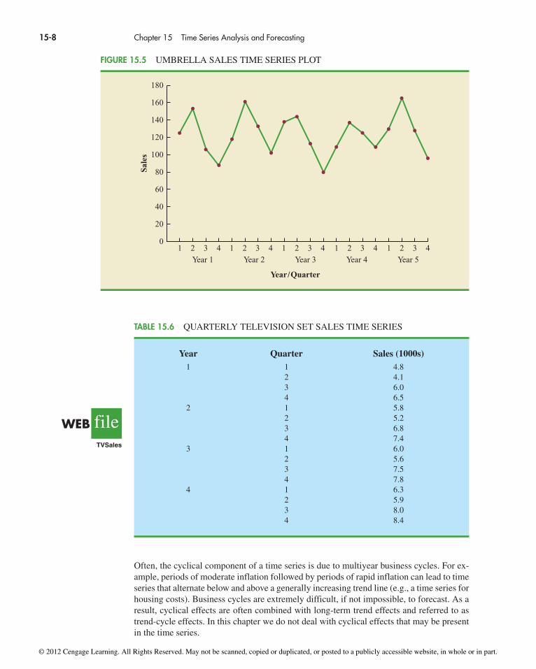
Once the actual time series value in period 3, Y3 � 19, is known, we can generate a fore-cast for period 4 as follows:
Continuing the exponential smoothing calculations, we obtain the weekly forecast val-ues shown in Table 15.10. Note that we have not shown an exponential smoothing forecastor a forecast error for week 1 because no forecast was made. For week 12, we have Y12 � 22and F12 � 18.48. We can we use this information to generate a forecast for week 13.
Thus, the exponential smoothing forecast of the amount sold in week 13 is 19.18, or 19,180 gallons of gasoline. With this forecast, the firm can make plans and decisionsaccordingly.
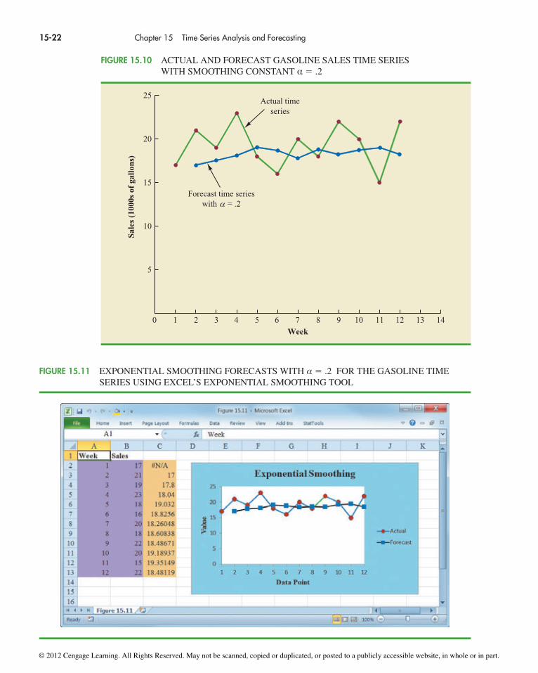
Figure 15.10 shows the time series plot of the actual and forecast time series values.Note in particular how the forecasts “smooth out” the irregular or random fluctuations inthe time series.
Using Excel’s Exponential Smoothing ToolThe following steps describe how to use Excel’s Exponential Smoothing tool to developforecasts for the gasoline sales time series in Table 15.1 using a smoothing constant of α � .2. Refer to Figure 15.11 as we describe the tasks involved.
Step 1. Click the Data tab on the RibbonStep 2. In the Analysis group, click Data Analysis
F13 � .2Y12 � .8F12 � .2(22) � .8(18.48) � 19.18
F4 � .2Y3 � .8F3 � .2(19) � .8(17.8) � 18.04
Forecast SquaredWeek Time Series Value Forecast Error Forecast Error
1 172 21 17.00 4.00 16.003 19 17.80 1.20 1.444 23 18.04 4.96 24.605 18 19.03 �1.03 1.066 16 18.83 �2.83 8.017 20 18.26 1.74 3.038 18 18.61 �0.61 0.379 22 18.49 3.51 12.32
10 20 19.19 0.81 0.6611 15 19.35 �4.35 18.9212 22 18.48 3.52 12.39
Totals 10.92 98.80
TABLE 15.10 SUMMARY OF THE EXPONENTIAL SMOOTHING FORECASTS AND FORECAST ERRORS FOR THE GASOLINE SALES TIME SERIESWITH SMOOTHING CONSTANT α � .2
© 2012 Cengage Learning. All Rights Reserved. May not be scanned, copied or duplicated, or posted to a publicly accessible website, in whole or in part.
15-22 Chapter 15 Time Series Analysis and Forecasting
Sale
s (1
000s
of
gallo
ns)
0
20
15
10
5
4 7 9
Week
25
1 2 3 65 8 10 1211 13 14
Actual timeseries
Forecast time serieswith = .2α
FIGURE 15.10 ACTUAL AND FORECAST GASOLINE SALES TIME SERIES WITH SMOOTHING CONSTANT α � .2
FIGURE 15.11 EXPONENTIAL SMOOTHING FORECASTS WITH α � .2 FOR THE GASOLINE TIMESERIES USING EXCEL’S EXPONENTIAL SMOOTHING TOOL
© 2012 Cengage Learning. All Rights Reserved. May not be scanned, copied or duplicated, or posted to a publicly accessible website, in whole or in part.

15.3 Moving Averages and Exponential Smoothing 15-23
Step 3. Choose Exponential Smoothing from the list of Analysis ToolsStep 4. When the Exponential Smoothing dialog box appears,
Enter B2:B13 in the Input Range boxEnter .8 in the Damping factor boxEnter C3 in the Output Range boxSelect Chart OutputClick OK
The exponential smoothing forecasts appear in column C of the worksheet. Note that thevalue we entered in the Damping factor box is 1 – α; forecasts for other smoothing constantscan be computed easily by entering a different value for 1 – α in the Damping factor box.
Forecast accuracy In the preceding exponential smoothing calculations, we used asmoothing constant of α � .2. Although any value of α between 0 and 1 is acceptable, somevalues will yield better forecasts than others. Insight into choosing a good value for α canbe obtained by rewriting the basic exponential smoothing model as follows:
(15.3)
Thus, the new forecast Ft�1 is equal to the previous forecast Ft plus an adjustment, whichis the smoothing constant α times the most recent forecast error, Yt � Ft. That is, the fore-cast in period t � 1 is obtained by adjusting the forecast in period t by a fraction of theforecast error. If the time series contains substantial random variability, a small value of thesmoothing constant is preferred. The reason for this choice is that if much of the forecasterror is due to random variability, we do not want to overreact and adjust the forecasts tooquickly. For a time series with relatively little random variability, forecast errors are morelikely to represent a change in the level of the series. Thus, larger values of the smoothingconstant provide the advantage of quickly adjusting the forecasts; this allows the forecaststo react more quickly to changing conditions.
The criterion we will use to determine a desirable value for the smoothing constantα is the same as the criterion we proposed for determining the order or number of peri-ods of data to include in the moving averages calculation. That is, we choose the valueof α that minimizes the MSE. A summary of the MSE calculations for the exponentialsmoothing forecast of gasoline sales with α � .2 is shown in Table 15.10. Note that thereis one less squared error term than the number of time periods because we had no pastvalues with which to make a forecast for period 1. The value of the sum of squaredforecast errors is 98.80; hence MSE � 98.80/11 � 8.98. Would a different value of αprovide better results in terms of a lower MSE value? Perhaps the most straightforwardway to answer this question is simply to try another value for α. We will then compareits mean squared error with the MSE value of 8.98 obtained by using a smoothingconstant of α � .2.
The exponential smoothing results with α � .3 are shown in Table 15.11. The value ofthe sum of squared forecast errors is 102.83; hence MSE � 102.83/11 � 9.35. WithMSE � 9.35, we see that, for the current data set, a smoothing constant of α � .3 resultsin less forecast accuracy than a smoothing constant of α � .2. Thus, we would be inclinedto prefer the original smoothing constant of α � .2. Using a trial-and-error calculation withother values of α, we can find a “good” value for the smoothing constant. This value can beused in the exponential smoothing model to provide forecasts for the future. At a later date,after new time series observations are obtained, we can analyze the newly collected timeseries data to determine whether the smoothing constant should be revised to providebetter forecasting results.
Ft�1 � αYt � (1 � α)Ft
Ft�1 � αYt � Ft � αFt
Ft�1 � Ft � α(Yt � Ft)
© 2012 Cengage Learning. All Rights Reserved. May not be scanned, copied or duplicated, or posted to a publicly accessible website, in whole or in part.

Exercises
Methods5. Consider the following time series data.
Week 1 2 3 4 5 6
Value 18 13 16 11 17 14
a. Construct a time series plot. What type of pattern exists in the data?b. Develop the three-week moving average forecasts for this time series. Compute MSE
and a forecast for week 7.
15-24 Chapter 15 Time Series Analysis and Forecasting
Forecast SquaredWeek Time Series Value Forecast Error Forecast Error
1 172 21 17.00 4.00 16.003 19 18.20 0.80 0.644 23 18.44 4.56 20.795 18 19.81 �1.81 3.286 16 19.27 �3.27 10.697 20 18.29 1.71 2.928 18 18.80 �0.80 0.649 22 18.56 3.44 11.83
10 20 19.59 0.41 0.1711 15 19.71 �4.71 22.1812 22 18.30 3.70 13.69
Totals 8.03 102.83
TABLE 15.11 SUMMARY OF THE EXPONENTIAL SMOOTHING FORECASTS ANDFORECAST ERRORS FOR THE GASOLINE SALES TIME SERIES WITHSMOOTHING CONSTANT α � .3
NOTES AND COMMENTS
1. Spreadsheet packages are an effective aid inchoosing a good value of α for exponentialsmoothing. With the time series data and theforecasting formulas in a spreadsheet, you canexperiment with different values of α andchoose the value that provides the smallest fore-cast error using one or more of the measures offorecast accuracy (MAE, MSE, or MAPE).
2. We presented the moving average and exponen-tial smoothing methods in the context of a
stationary time series. These methods can alsobe used to forecast a nonstationary time serieswhich shifts in level but exhibits no trend or sea-sonality. Moving averages with small values ofk adapt more quickly than moving averages withlarger values of k. Exponential smoothing mod-els with smoothing constants closer to one adaptmore quickly than models with smaller valuesof the smoothing constant.
testSELF
© 2012 Cengage Learning. All Rights Reserved. May not be scanned, copied or duplicated, or posted to a publicly accessible website, in whole or in part.

15.3 Moving Averages and Exponential Smoothing 15-25
c. Use α � .2 to compute the exponential smoothing forecasts for the time series. Com-pute MSE and a forecast for week 7.
d. Compare the three-week moving average approach with the exponential smoothingapproach using α � .2. Which appears to provide more accurate forecasts based onMSE? Explain.
e. Use a smoothing constant of α � .4 to compute the exponential smoothing forecasts.Does a smoothing constant of .2 or .4 appear to provide more accurate forecasts basedon MSE? Explain.
6. Consider the following time series data.
Month 1 2 3 4 5 6 7
Value 24 13 20 12 19 23 15
Construct a time series plot. What type of pattern exists in the data?a. Develop the three-week moving average forecasts for this time series. Compute MSE
and a forecast for week 8.b. Use α � .2 to compute the exponential smoothing forecasts for the time series. Com-
pute MSE and a forecast for week 8.c. Compare the three-week moving average approach with the exponential smoothing
approach using α � .2. Which appears to provide more accurate forecasts based on MSE?d. Use a smoothing constant of α � .4 to compute the exponential smoothing forecasts.
Does a smoothing constant of .2 or .4 appear to provide more accurate forecasts basedon MSE? Explain.
7. Refer to the gasoline sales time series data in Table 15.1.a. Compute four-week and five-week moving averages for the time series.b. Compute the MSE for the four-week and five-week moving average forecasts.c. What appears to be the best number of weeks of past data (three, four, or five) to use
in the moving average computation? Recall that MSE for the three-week moving average is 10.22.
8. Refer again to the gasoline sales time series data in Table 15.1.a. Using a weight of 1/2 for the most recent observation, 1/3 for the second most recent
observation, and 1/6 for third most recent observation, compute a three-week weightedmoving average for the time series.
b. Compute the MSE for the weighted moving average in part (a). Do you prefer thisweighted moving average to the unweighted moving average? Remember that theMSE for the unweighted moving average is 10.22.
c. Suppose you are allowed to choose any weights as long as they sum to 1. Could youalways find a set of weights that would make the MSE at least as small for aweighted moving average than for an unweighted moving average? Why or whynot?
9. With the gasoline time series data from Table 15.1, show the exponential smoothing fore-casts using α � .1.a. Applying the MSE measure of forecast accuracy, would you prefer a smoothing con-
stant of α � .1 or α � .2 for the gasoline sales time series?b. Are the results the same if you apply MAE as the measure of accuracy?c. What are the results if MAPE is used?
10. With a smoothing constant of α � .2, equation (15.2) shows that the forecast for week 13of the gasoline sales data from Table 15.1 is given by F13 � .2Y12 + .8F12. However, theforecast for week 12 is given by F12 � .2Y11 + .8F11. Thus, we could combine these tworesults to show that the forecast for week 13 can be written
F13 � .2Y12 � .8(.2Y11 � .8F11) � .2Y12 � .16Y11 � .64Y11 � .64F11
fileWEBGasoline
fileWEBGasoline
fileWEBGasoline
© 2012 Cengage Learning. All Rights Reserved. May not be scanned, copied or duplicated, or posted to a publicly accessible website, in whole or in part.

a. Making use of the fact that F11 � .2Y10 + .8F10 (and similarly for F10 and F9), continueto expand the expression for F13 until it is written in terms of the past data values Y12,Y11, Y10, Y9, Y8, and the forecast for period 8.
b. Refer to the coefficients or weights for the past values Y12, Y11, Y10, Y9, Y8. Whatobservation can you make about how exponential smoothing weights past data valuesin arriving at new forecasts? Compare this weighting pattern with the weighting patternof the moving averages method.
Applications11. For the Hawkins Company, the monthly percentages of all shipments received on time
over the past 12 months are 80, 82, 84, 83, 83, 84, 85, 84, 82, 83, 84, and 83.a. Construct a time series plot. What type of pattern exists in the data?b. Compare the three-month moving average approach with the exponential smooth-
ing approach for α � .2. Which provides more accurate forecasts using MSE as themeasure of forecast accuracy?
c. What is the forecast for next month?
12. Corporate triple-A bond interest rates for 12 consecutive months follow.
9.5 9.3 9.4 9.6 9.8 9.7 9.8 10.5 9.9 9.7 9.6 9.6
a. Construct a time series plot. What type of pattern exists in the data?b. Develop three-month and four-month moving averages for this time series. Does the
three-month or four-month moving average provide more accurate forecasts basedon MSE? Explain.
c. What is the moving average forecast for the next month?
13. The values of Alabama building contracts (in $ millions) for a 12-month period follow.
240 350 230 260 280 320 220 310 240 310 240 230
a. Construct a time series plot. What type of pattern exists in the data?b. Compare the three-month moving average approach with the exponential smoothing
forecast using α � .2. Which provides more accurate forecasts based on MSE?c. What is the forecast for the next month?
14. The following time series shows the sales of a particular product over the past 12 months.
15-26 Chapter 15 Time Series Analysis and Forecasting
Month Sales Month Sales
1 105 7 1452 135 8 1403 120 9 1004 105 10 805 90 11 1006 120 12 110
a. Construct a time series plot. What type of pattern exists in the data?b. Use α � .3 to compute the exponential smoothing forecasts for the time series.c. Use a smoothing constant of α � .5 to compute the exponential smoothing forecasts.
Does a smoothing constant of .3 or .5 appear to provide more accurate forecasts basedon MSE?
15. Ten weeks of data on the Commodity Futures Index are 7.35, 7.40, 7.55, 7.56, 7.60, 7.52,7.52, 7.70, 7.62, and 7.55.a. Construct a time series plot. What type of pattern exists in the data?b. Compute the exponential smoothing forecasts for α � .2.
testSELF
© 2012 Cengage Learning. All Rights Reserved. May not be scanned, copied or duplicated, or posted to a publicly accessible website, in whole or in part.

15.4 Trend Projection 15-27
c. Compute the exponential smoothing forecasts for α � .3.d. Which exponential smoothing constant provides more accurate forecasts based on
MSE? Forecast week 11.
16. The Nielsen ratings (percentage of U.S. households that tuned in) for the Masters GolfTournament from 1997 through 2008 follow (Golf Magazine, January 2009).
fileWEBMasters
Year Rating
1997 11.21998 8.61999 7.92000 7.62001 10.72002 8.12003 6.92004 6.72005 8.02006 6.92007 7.62008 7.3
The rating of 11.2 in 1997 indicates that 11.2% of U.S. households tuned in to watch TigerWoods win his first major golf tournament and become the first African American to winthe Masters. Tiger Woods also won the Masters in 2001 and 2005. a. Construct a time series plot. What type of pattern exists in the data? Discuss some of
the factors that may have resulted in the pattern exhibited in the time series plot forthis time series.
b. Given the pattern of the time series plot developed in part (a), do you think the fore-casting methods discussed in this section are appropriate to develop forecasts for thistime series? Explain.
c. Would you recommend using the Nielsen ratings for only 2002–2008 to forecast therating for 2009, or should the entire time series from 1997–2008 be used? Explain.
Trend ProjectionWe present forecasting methods in this section that are appropriate for time series ex-hibiting a trend pattern. First, we show how simple linear regression can be used to fore-cast a time series with a linear trend. We then show how the curve-fitting capability ofregression analysis can also be used to forecast time series with a curvilinear or nonlineartrend.
Linear Trend RegressionIn Section 15.1 we used the bicycle sales time series in Table 15.3 and Figure 15.3 toillustrate a time series with a trend pattern. Let us now use this time series to illustrate howsimple linear regression can be used to forecast a time series with a linear trend. The datafor the bicycle time series are repeated in Table 15.12 and Figure 15.12.
Although the time series plot in Figure 15.12 shows some up and down movement overthe past 10 years, we might agree that the linear trend line shown in Figure 15.13 provides areasonable approximation of the long-run movement in the series. We can use the methods
15.4
fileWEBBicycle
TABLE 15.12BICYCLE SALESTIME SERIES
Year Sales (1000s)1 21.62 22.93 25.54 21.95 23.96 27.57 31.58 29.79 28.6
10 31.4
© 2012 Cengage Learning. All Rights Reserved. May not be scanned, copied or duplicated, or posted to a publicly accessible website, in whole or in part.
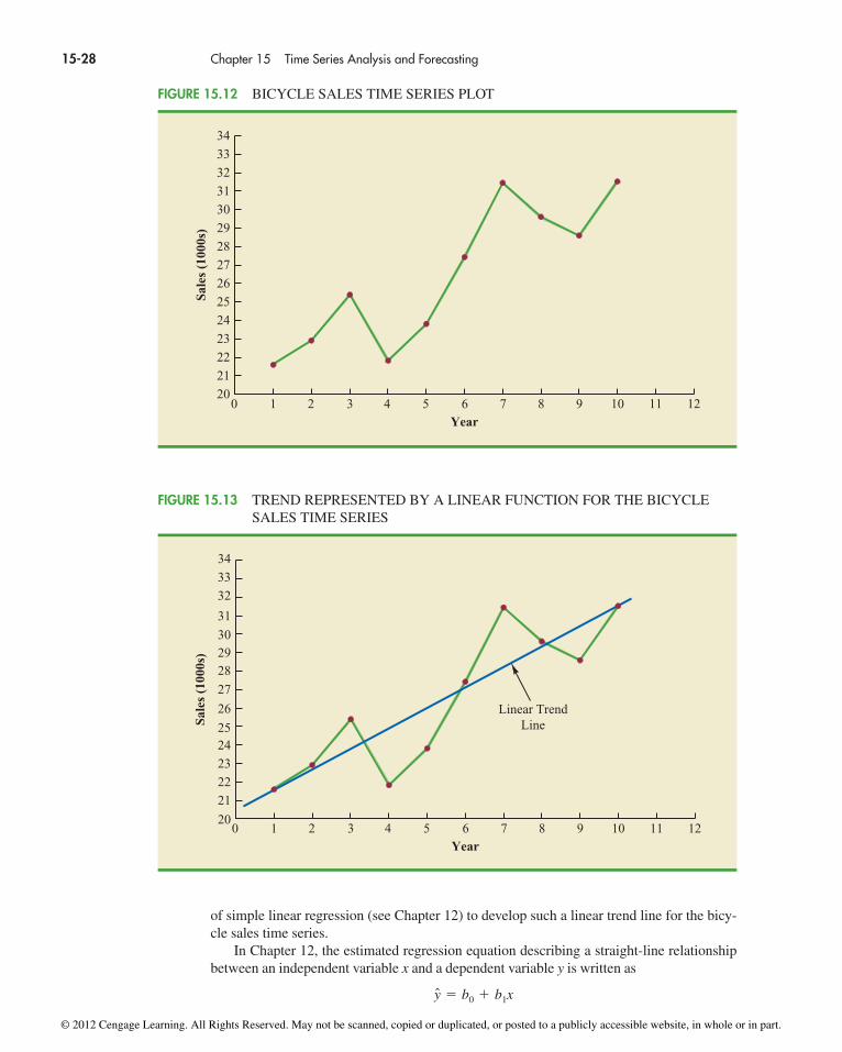
of simple linear regression (see Chapter 12) to develop such a linear trend line for the bicy-cle sales time series.
In Chapter 12, the estimated regression equation describing a straight-line relationshipbetween an independent variable x and a dependent variable y is written as
y � b0 � b1x
15-28 Chapter 15 Time Series Analysis and Forecasting
Sale
s (1
000s
)
0
32
33
34
27
25
4 7 9Year
1 2 3 65 8 10 11 12
31
30
29
28
26
24
23
22
21
20
FIGURE 15.12 BICYCLE SALES TIME SERIES PLOT
Sale
s (1
000s
)
0
32
33
34
27
25
4 7 9Year
1 2 3 65 8 10 11 12
31
30
2928
26
24
23
22
21
20
Linear TrendLine
FIGURE 15.13 TREND REPRESENTED BY A LINEAR FUNCTION FOR THE BICYCLESALES TIME SERIES
© 2012 Cengage Learning. All Rights Reserved. May not be scanned, copied or duplicated, or posted to a publicly accessible website, in whole or in part.

15.4 Trend Projection 15-29
where is the predicted value of y. To emphasize the fact that in forecasting the independentvariable is time, we will replace x with t and with Tt to emphasize that we are estimatingthe trend for a time series. Thus, for estimating the linear trend in a time series we will usethe following estimated regression equation.
yy
LINEAR TREND EQUATION
(15.4)
where
Tt �
b0 �
b1 �
t �
linear trend forecast in period t
intercept of the linear trend line
slope of the linear trend line
time period
Tt � b0 � b1t
In equation (15.4), the time variable begins at t � 1 corresponding to the first time seriesobservation (year 1 for the bicycle sales time series) and continues until t � n correspond-ing to the most recent time series observation (year 10 for the bicycle sales time series).Thus, for the bicycle sales time series t � 1 corresponds to the oldest time series value andt � 10 corresponds to the most recent year.
Formulas for computing the estimated regression coefficients (b1 and b0) in equation(15.4) follow.
COMPUTING THE SLOPE AND INTERCEPT FOR A LINEAR TREND*
where
*An alternate formula for b1 is
This form of equation (15.5) is often recommended when using a calculator to compute b1.
b1 ��
n
t�1
tYt � � �n
t�1
t �n
t�1
Yt� �n
�n
t�1
t 2 � � �n
t�1
t�2
�n
Yt �
n �
Y �
t �
value of the time series in period t
number of time periods (number of observations)
average value of the time series
average value of t
(15.5)
(15.6)
b1 ��(
n
t�1
t � t )(Yt � Y)
�n
t�1
(t � t )2
b0 � Y � b1t
© 2012 Cengage Learning. All Rights Reserved. May not be scanned, copied or duplicated, or posted to a publicly accessible website, in whole or in part.

To compute the linear trend equation for the bicycle sales time series, we begin the cal-culations by computing and using the information in Table 15.12.
Using these values, and the information in Table 15.13, we can compute the slope andintercept of the trend line for the bicycle sales time series.
Therefore, the linear trend equation is
The slope of 1.1 indicates that over the past 10 years the firm experienced an averagegrowth in sales of about 1100 units per year. If we assume that the past 10-year trend insales is a good indicator of the future, this trend equation can be used to develop forecastsfor future time periods. For example, substituting t � 11 into the equation yields next year’strend projection or forecast, T11.
Thus, using trend projection, we would forecast sales of 32,500 bicycles next year.
T11 � 20.4 � 1.1(11) � 32.5
Tt � 20.4 � 1.1t
b0 � Y � b1t � 26.45 � 1.1(5.5) � 20.4
b1 ��
n
t�1
(t � t )(Yt � Y )
�n
t�1
(t � t )2
�90.75
82.5� 1.1
Y ��
n
t�1
Yt
n�
264.5
10� 26.45
t ��
n
t�1
t
n�
55
10� 5.5
Yt
15-30 Chapter 15 Time Series Analysis and Forecasting
t Y1 t � Yt � (t � )(Yt � ) (t � )2
1 21.6 �4.5 �4.85 21.825 20.252 22.9 �3.5 �3.55 12.425 12.253 25.5 �2.5 �0.95 2.375 6.254 21.9 �1.5 �4.55 6.825 2.255 23.9 �0.5 �2.55 1.275 0.256 27.5 0.5 1.05 0.525 0.257 31.5 1.5 5.05 7.575 2.258 29.7 2.5 3.25 8.125 6.259 28.6 3.5 2.15 7.525 12.25
10 31.4 4.5 4.95 22.275 20.25
Totals 55 264.5 90.750 82.50
tYtYt
TABLE 15.13 SUMMARY OF LINEAR TREND CALCULATIONS FOR THE BICYCLE SALESTIME SERIES
© 2012 Cengage Learning. All Rights Reserved. May not be scanned, copied or duplicated, or posted to a publicly accessible website, in whole or in part.

15.4 Trend Projection 15-31
To compute the accuracy associated with the trend projection forecasting method, we willuse the MSE. Table 15.14 shows the computation of the sum of squared errors for the bicyclesales time series. Thus, for the bicycle sales time series,
Using Excel’s Regression Tool to Compute a Linear Trend EquationIn Section 12.7 we showed how Excel’s Regression tool can be used to perform a completeregression analysis. The same procedure can be used to compute a linear trend equation. Weillustrate using the bicycle sales time series in Table 15.12. Refer to Figure 15.14 as we describethe tasks involved.
Step 1. Click the Data tab on the RibbonStep 2. In the Analysis group, click Data AnalysisStep 3. Choose Regression from the list of Analysis ToolsStep 4. When the Regression dialog box appears,
Enter B1:B11 in the Input Y Range boxEnter A1:A11 in the Input X Range boxSelect LabelsSelect Confidence LevelEnter 99 in the Confidence Level boxSelect Output RangeEnter A13 in the Output Range box (to identify the upper left corner of the
section of the worksheet where the output will appear)Click OK
The Excel Regression tool output shows that the value of the intercept of the trend line is 20.4(cell B29) and that the slope of the trend line is 1.1 (cell B30), the same values we obtainedusing hand caclulation. But in the regression output the value of MSE (cell D25) is
MSE �Sum of Squares Due to Error
Degrees of Freedom�
30.7
8� 3.8375
MSE ��
n
t�1(Yt � Ft )2
n�
30.7
10� 3.07
fileWEBBicycle
SquaredYear Sales (1000s) Yt Forecast Tt Forecast Error Forecast Error
1 21.6 21.5 0.1 0.012 22.9 22.6 0.3 0.093 25.5 23.7 1.8 3.244 21.9 24.8 �2.9 8.415 23.9 25.9 �2.0 4.006 27.5 27.0 0.5 0.257 31.5 28.1 3.4 11.568 29.7 29.2 0.5 0.259 28.6 30.3 �1.7 2.89
10 31.4 31.4 0.0 0.00
Total 30.70
TABLE 15.14 SUMMARY OF THE LINEAR TREND FORECASTS AND FORECASTERRORS FOR THE BICYCLE SALES TIME SERIES
© 2012 Cengage Learning. All Rights Reserved. May not be scanned, copied or duplicated, or posted to a publicly accessible website, in whole or in part.
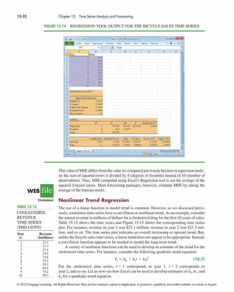
This value of MSE differs from the value we computed previously because in regression analy-sis the sum of squared errors is divided by 8 (degrees of freedom) instead of 10 (number ofobservations). Thus, MSE computed using Excel’s Regression tool is not the average of thesquared forecast errors. Most forecasting packages, however, compute MSE by taking theaverage of the forecast errors.
Nonlinear Trend RegressionThe use of a linear function to model trend is common. However, as we discussed previ-ously, sometimes time series have a curvilinear or nonlinear trend. As an example, considerthe annual revenue in millions of dollars for a cholesterol drug for the first 10 years of sales.Table 15.15 shows the time series and Figure 15.15 shows the corresponding time seriesplot. For instance, revenue in year 1 was $23.1 million; revenue in year 2 was $21.3 mil-lion; and so on. The time series plot indicates an overall increasing or upward trend. But,unlike the bicycle sales time series, a linear trend does not appear to be appropriate. Instead,a curvilinear function appears to be needed to model the long-term trend.
A variety of nonlinear functions can be used to develop an estimate of the trend for thecholesterol time series. For instance, consider the following quadratic trend equation:
(15.7)
For the cholesterol time series, t � 1 corresponds to year 1, t � 2 corresponds to year 2, and so on. Let us now see how Excel can be used to develop estimates of b0, b1, andb2 for a quadratic trend equation.
Tt � b0 � b1t � b2t2
15-32 Chapter 15 Time Series Analysis and Forecasting
FIGURE 15.14 REGRESSION TOOL OUTPUT FOR THE BICYCLE SALES TIME SERIES
TABLE 15.15CHOLESTEROLREVENUETIME SERIES($MILLIONS)
Year Revenue(t) ($millions)
1 23.12 21.33 27.44 34.65 33.86 43.27 59.58 64.49 74.2
10 99.3
fileWEBCholesterol
© 2012 Cengage Learning. All Rights Reserved. May not be scanned, copied or duplicated, or posted to a publicly accessible website, in whole or in part.

15.4 Trend Projection 15-33
Using Excel’s Regression Tool to Compute a QuadraticTrend EquationWe can use Excel’s Regression tool to compute a quadratic trend equation by creating amultiple regression model consisting of two independent variables, year and yearsquared. We illustrate using the cholesterol revenue time series in Table 15.15. Refer toFigure 15.16 as we describe the tasks involved. Note that Column A contains the valuesfor year, in column B we have computed the values of year squared, and column C con-tains the values of the dependent variable, sales revenue in millions of dollars. Thus, thefirst observation is 1, 1, 23.1; the second observation is 2, 4, 21.3; the third observationis 3, 9, 27.4; and so on.
Step 1. Click the Data tab on the RibbonStep 2. In the Analysis group, click Data AnalysisStep 3. Choose Regression from the list of Analysis ToolsStep 4. When the Regression dialog box appears,
Enter C1:C11 in the Input Y Range boxEnter A1:B11 in the Input X Range box
Select LabelsSelect Confidence LevelEnter 99 in the Confidence Level boxSelect Output RangeEnter A13 in the Output Range box (to identify the upper left corner of
the section of the worksheet where the output will appear)Click OK
The Excel Regression tool output shows that the values of b0, b1, and b2 are 24.1817(cell B29), �2.1060 (cell B30), and 0.9216 (cell B31). Thus, the estimated regressionequation is
Tt � 24.1817 � 2.1060t � 0.9216t2
Rev
enue
120
4 7 9Year
0 1 2 3 65 8 10
100
80
60
40
20
0
FIGURE 15.15 CHOLESTEROL REVENUE TIMES SERIES PLOT ($MILLIONS)
© 2012 Cengage Learning. All Rights Reserved. May not be scanned, copied or duplicated, or posted to a publicly accessible website, in whole or in part.

Thus, a forecast of sales revenue for year 11 is
Tt � 24.1817 � 2.1060(11) � 0.9216(11)2 � 112.53
or approximately $112.5 million.
Using Excel’s Chart Tools for Trend ProjectionIn closing this section we show how Excel’s chart tools can be used to develop a variety oftrend equations, including linear, polynomial, and exponential. We illustrate by computinga quadratic trend equation for the cholesterol drug revenue time series in Table 15.15.
First, we create a time series plot (without lines connecting the points) for the choles-terol time series. The resulting Excel chart is shown in Figure 15.17. Refer to Figure 15.17as we describe the tasks involved in developing a quadratic trend line.
Step 1. Position the mouse pointer over any data point in the scatter diagram and right-click to display a list of options; choose Add Trendline
Step 2. When the Format Trendline dialog box appears (see Figure 15.18),Select Trendline Options and then
Choose Polynomial from the Trend/Regression Type listEnter 2 in the Order boxChoose Display Equation on chart Click Close
15-34 Chapter 15 Time Series Analysis and Forecasting
FIGURE 15.16 REGRESSION TOOL OUTPUT FOR THE CHOLESTEROL REVENUE TIME SERIES
© 2012 Cengage Learning. All Rights Reserved. May not be scanned, copied or duplicated, or posted to a publicly accessible website, in whole or in part.

15.4 Trend Projection 15-35
FIGURE 15.17 USING EXCEL’S CHART TOOLS TO COMPUTE A TIME SERIES PLOT FORTHE CHOLESTEROL REVENUE TIME SERIES
FIGURE 15.18 EXCEL’S FORMAT TRENDLINE DIALOG BOX FOR THE CHOLESTEROLREVENUE TIME SERIES
© 2012 Cengage Learning. All Rights Reserved. May not be scanned, copied or duplicated, or posted to a publicly accessible website, in whole or in part.

Figure 15.18 shows that there are six options for the type of trend line. Choosing the polyno-mial option with order 2 indicates that we want to fit a quadratic trend equation (a second-degree polynomial) to the data. The worksheet displayed in Figure 15.19 shows the timeseries plot, the quadratic trend equation, and the graph of the trend equation.
Except for rounding, the trend equation computed using Excel’s chart tools is the sameas the trend equation we computed using Excel’s Regression tool. And it is much easier tofit a variety of trend lines to a time series using this approach. However, the advantage ofusing Excel’s Regression tool for trend projection is that it provides additional output thatcan be used to determine the statistical significance of the trend equation as well as deter-mine how good a fit the estimated regression equation provides.
Exercises
Methods17. Consider the following time series data.
t 1 2 3 4 5
Yt 6 11 9 14 15
a. Construct a time series plot. What type of pattern exists in the data?b. Develop the linear trend equation for this time series.c. What is the forecast for t � 6?
15-36 Chapter 15 Time Series Analysis and Forecasting
A quadratic trend equationis simply a second-degreepolynomial function.
FIGURE 15.19 USING EXCEL’S CHART TOOLS TO COMPUTE A QUADRATIC TREND EQUATION FOR THE CHOLESTEROL REVENUE TIME SERIES
testSELF
© 2012 Cengage Learning. All Rights Reserved. May not be scanned, copied or duplicated, or posted to a publicly accessible website, in whole or in part.
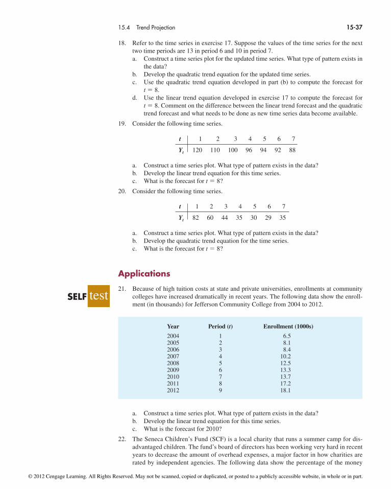
15.4 Trend Projection 15-37
18. Refer to the time series in exercise 17. Suppose the values of the time series for the nexttwo time periods are 13 in period 6 and 10 in period 7.a. Construct a time series plot for the updated time series. What type of pattern exists in
the data?b. Develop the quadratic trend equation for the updated time series.c. Use the quadratic trend equation developed in part (b) to compute the forecast for
t � 8.d. Use the linear trend equation developed in exercise 17 to compute the forecast for
t � 8. Comment on the difference between the linear trend forecast and the quadratictrend forecast and what needs to be done as new time series data become available.
19. Consider the following time series.
t 1 2 3 4 5 6 7
Yt 120 110 100 96 94 92 88
a. Construct a time series plot. What type of pattern exists in the data?b. Develop the linear trend equation for this time series.c. What is the forecast for t � 8?
20. Consider the following time series.
t 1 2 3 4 5 6 7
Yt 82 60 44 35 30 29 35
a. Construct a time series plot. What type of pattern exists in the data?b. Develop the quadratic trend equation for the time series.c. What is the forecast for t � 8?
Applications
21. Because of high tuition costs at state and private universities, enrollments at communitycolleges have increased dramatically in recent years. The following data show the enroll-ment (in thousands) for Jefferson Community College from 2004 to 2012.
testSELF
Year Period (t) Enrollment (1000s)
2004 1 6.52005 2 8.12006 3 8.42007 4 10.22008 5 12.52009 6 13.32010 7 13.72011 8 17.22012 9 18.1
a. Construct a time series plot. What type of pattern exists in the data?b. Develop the linear trend equation for this time series.c. What is the forecast for 2010?
22. The Seneca Children’s Fund (SCF) is a local charity that runs a summer camp for dis-advantaged children. The fund’s board of directors has been working very hard in recentyears to decrease the amount of overhead expenses, a major factor in how charities arerated by independent agencies. The following data show the percentage of the money
© 2012 Cengage Learning. All Rights Reserved. May not be scanned, copied or duplicated, or posted to a publicly accessible website, in whole or in part.

SCF has raised that was spent on administrative and fund-raising expenses for2006–2012.
15-38 Chapter 15 Time Series Analysis and Forecasting
Year Cost/Unit ($) Year Cost/Unit ($)
1 20.00 5 26.602 24.50 6 30.003 28.20 7 31.004 27.50 8 36.00
Year Period (t) Expense (%)
2006 1 13.92007 2 12.22008 3 10.52009 4 10.42010 5 11.52011 6 10.02012 7 8.5
a. Construct a time series plot. What type of pattern exists in the data?b. Develop the linear trend equation for this time series.c. Forecast the percentage of administrative expenses for 2013.d. If SCF can maintain its current trend in reducing administrative expenses, how long
will it take it to achieve a level of 5% or less?
23. The president of a small manufacturing firm is concerned about the continual increase inmanufacturing costs over the past several years. The following figures provide a time seriesof the cost per unit for the firm’s leading product over the past eight years.
a. Construct a time series plot. What type of pattern exists in the data?b. Develop the linear trend equation for this time series.c. What is the average cost increase that the firm has been realizing per year?d. Compute an estimate of the cost/unit for next year.
24. FRED® (Federal Reserve Economic Data), a database of more than 3000 U.S. economictime series, contains historical data on foreign exchange rates. The following data show the foreign exchange rate for the United States and China (Federal Reserve Bank ofSt. Louis website). The units for Rate are the number of Chinese yuan to one U.S. dollar.
Year Month Rate
2007 October 7.50192007 November 7.42102007 December 7.36822008 January 7.24052008 February 7.16442008 March 7.07222008 April 6.99972008 May 6.97252008 June 6.89932008 July 6.8355
fileWEBExchangeRate
© 2012 Cengage Learning. All Rights Reserved. May not be scanned, copied or duplicated, or posted to a publicly accessible website, in whole or in part.

15.4 Trend Projection 15-39
a. Construct a time series plot. Does a linear trend appear to be present?b. Develop the linear trend equation for this time series. c. Use the trend equation to forecast the exchange rate for August 2008.d. Would you feel comfortable using the trend equation to forecast the exchange rate for
December 2008?
25. Automobile unit sales at B. J. Scott Motors, Inc., provided the following 10-year timeseries.
Year Sales Year Sales
1 400 6 2602 390 7 3003 320 8 3204 340 9 3405 270 10 370
a. Construct a time series plot. Comment on the appropriateness of a linear trend. b. Develop a quadratic trend equation that can be used to forecast sales.c. Using the trend equation developed in part (b), forecast sales in year 11.d. Suggest an alternative to using a quadratic trend equation to forecast sales. Explain.
26. Giovanni Food Products produces and sells frozen pizzas to public schools throughout theeastern United States. Using a very aggressive marketing strategy they have been able toincrease their annual revenue by approximately $10 million over the past 10 years. Butincreased competition has slowed their growth rate in the past few years. The annual revenue,in millions of dollars, for the previous 10 years is shown.
Year Revenue
1 8.532 10.843 12.984 14.115 16.316 17.217 18.378 18.459 18.40
10 18.43
fileWEBPasta
a. Construct a time series plot. Comment on the appropriateness of a linear trend. b. Develop a quadratic trend equation that can be used to forecast revenue.c. Using the trend equation developed in part (b), forecast revenue in year 11.
27. Forbes magazine ranks NFL teams by value each year. The following data are the value ofthe Indianapolis Colts from 1998 to 2008 (Forbes website).
Year Period Value ($millions)
1998 1 2271999 2 3052000 3 3322001 4 3672002 5 419
fileWEBNFLValue
© 2012 Cengage Learning. All Rights Reserved. May not be scanned, copied or duplicated, or posted to a publicly accessible website, in whole or in part.

a. Construct a time series plot. What type of pattern exists in the data?b. Develop a linear trend equation that can be used to forecast the team’s value.c. Develop a quadratic trend equation that can be used to forecast the team’s value.d. Which equation would you recommend using to estimate the team’s value in 2009?e. Use the model you recommended in part (d) to forecast the value of the Colts in 2009.
Seasonality and TrendIn this section we show how to develop forecasts for a time series that has a seasonal pattern.To the extent that seasonality exists, we need to incorporate it into our forecasting models toensure accurate forecasts. We begin by considering a seasonal time series with no trend andthen discuss how to model seasonality with trend.
Seasonality Without TrendAs an example, consider the number of umbrellas sold at a clothing store over the past fiveyears. Table 15.16 shows the time series and Figure 15.20 shows the corresponding time series plot. The time series plot does not indicate any long-term trend in sales. In fact, unless you look carefully at the data, you might conclude that the data follow a horizontalpattern and that single exponential smoothing could be used to forecast sales. But closerinspection of the time series plot reveals a pattern in the data. That is, the first and third quarters have moderate sales, the second quarter has the highest sales, and the fourth quar-ter tends to be the lowest quarter in terms of sales volume. Thus, we would conclude that aquarterly seasonal pattern is present.
In Chapter 13 we showed how dummy variables can be used to deal with categoricalindependent variables in a multiple regression model. We can use the same approach tomodel a time series with a seasonal pattern by treating the season as a categorical vari-able. Recall that when a categorical variable has k levels, k � 1 dummy variables arerequired. So, if there are four seasons, we need three dummy variables. For instance, inthe umbrella sales time series season is a categorical variable with four levels: quarter 1,quarter 2, quarter 3, and quarter 4. Thus, to model the seasonal effects in the umbrellatime series we need 4 � 1 � 3 dummy variables. The three dummy variables can be codedas follows:
Using to denote the estimated or forecasted value of sales, the general form of thepredicted regression equation relating the number of umbrellas sold to the quarter the salestake place follows:
Y � b0 � b1 Qtr1 � b2 Qtr2 � b3 Qtr3
Y
Qtr3 � �1 if Quarter 3
0 otherwiseQtr2 � �1 if Quarter 2
0 otherwiseQtr1 � �1 if Quarter 1
0 otherwise
15.5
15-40 Chapter 15 Time Series Analysis and Forecasting
Year Period Value ($millions)
2003 6 5472004 7 6092005 8 7152006 9 8372007 10 9112008 11 1076
fileWEBUmbrella
TABLE 15.16UMBRELLA SALESTIME SERIES
Year Quarter Sales1 1 125
2 1533 1064 88
2 1 1182 1613 1334 102
3 1 1382 1443 1134 80
4 1 1092 1373 1254 109
5 1 1302 1653 1284 96
© 2012 Cengage Learning. All Rights Reserved. May not be scanned, copied or duplicated, or posted to a publicly accessible website, in whole or in part.

15.5 Seasonality and Trend 15-41
Table 15.17 is the umbrella sales time series with the coded values of the dummy variablesshown. Using the data in Table 15.17 and Excel’s Regression tool, we obtained the computeroutput shown in Figure 15.21. The estimated multiple regression equation obtained is
We can use this equation to forecast quarterly sales for next year.
It is interesting to note that we could have obtained the quarterly forecasts for next yearsimply by computing the average number of umbrellas sold in each quarter, as shown in thefollowing table.
Quarter 1: Sales � 95.0 � 29.0(1) � 57.0(0) � 26.0(0) � 124
Quarter 2: Sales � 95.0 � 29.0(0) � 57.0(1) � 26.0(0) � 152
Quarter 3: Sales � 95.0 � 29.0(0) � 57.0(0) � 26.0(1) � 121
Quarter 4: Sales � 95.0 � 29.0(0) � 57.0(1) � 26.0(0) � 95
Sales � 95.0 � 29.0 Qtr1 � 57.0 Qtr2 � 26.0 Qtr3
Year Quarter 1 Quarter 2 Quarter 3 Quarter 4
1 125 153 106 882 118 161 133 1023 138 144 113 804 109 137 125 1095 130 165 128 96
Average 124 152 121 95
Sale
s
180
160
4 3 1 2 3 4 1 2 3 4 1 2 3 41 2 3 21 4
140
100
120
80
60
40
20
0
Year 1 Year 2 Year 3 Year 4 Year 5
Year/Quarter
FIGURE 15.20 UMBRELLA SALES TIME SERIES PLOT
Nonetheless, the regression output shown in Figure 15.21 provides additional informationthat can be used to assess the accuracy of the forecast and determine the significance of the
© 2012 Cengage Learning. All Rights Reserved. May not be scanned, copied or duplicated, or posted to a publicly accessible website, in whole or in part.
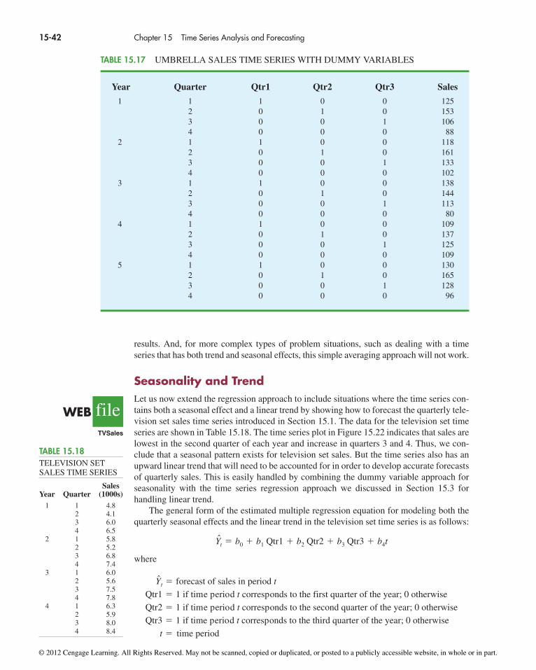
15-42 Chapter 15 Time Series Analysis and Forecasting
Year Quarter Qtr1 Qtr2 Qtr3 Sales
1 1 1 0 0 1252 0 1 0 1533 0 0 1 1064 0 0 0 88
2 1 1 0 0 1182 0 1 0 1613 0 0 1 1334 0 0 0 102
3 1 1 0 0 1382 0 1 0 1443 0 0 1 1134 0 0 0 80
4 1 1 0 0 1092 0 1 0 1373 0 0 1 1254 0 0 0 109
5 1 1 0 0 1302 0 1 0 1653 0 0 1 1284 0 0 0 96
TABLE 15.17 UMBRELLA SALES TIME SERIES WITH DUMMY VARIABLES
results. And, for more complex types of problem situations, such as dealing with a time series that has both trend and seasonal effects, this simple averaging approach will not work.
Seasonality and TrendLet us now extend the regression approach to include situations where the time series con-tains both a seasonal effect and a linear trend by showing how to forecast the quarterly tele-vision set sales time series introduced in Section 15.1. The data for the television set timeseries are shown in Table 15.18. The time series plot in Figure 15.22 indicates that sales arelowest in the second quarter of each year and increase in quarters 3 and 4. Thus, we con-clude that a seasonal pattern exists for television set sales. But the time series also has anupward linear trend that will need to be accounted for in order to develop accurate forecastsof quarterly sales. This is easily handled by combining the dummy variable approach forseasonality with the time series regression approach we discussed in Section 15.3 forhandling linear trend.
The general form of the estimated multiple regression equation for modeling both thequarterly seasonal effects and the linear trend in the television set time series is as follows:
where
Yt � forecast of sales in period t
Qtr1 � 1 if time period t corresponds to the first quarter of the year; 0 otherwise
Qtr2 � 1 if time period t corresponds to the second quarter of the year; 0 otherwise
Qtr3 � 1 if time period t corresponds to the third quarter of the year; 0 otherwise
t � time period
Yt � b0 � b1 Qtr1 � b2 Qtr2 � b3 Qtr3 � b4t
fileWEBTVSales
TABLE 15.18TELEVISION SETSALES TIME SERIES
SalesYear Quarter (1000s)
1 1 4.82 4.13 6.04 6.5
2 1 5.82 5.23 6.84 7.4
3 1 6.02 5.63 7.54 7.8
4 1 6.32 5.93 8.04 8.4
© 2012 Cengage Learning. All Rights Reserved. May not be scanned, copied or duplicated, or posted to a publicly accessible website, in whole or in part.
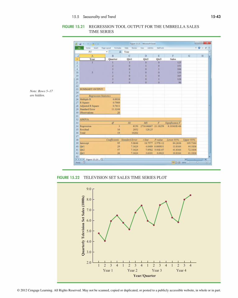
15.5 Seasonality and Trend 15-43
FIGURE 15.21 REGRESSION TOOL OUTPUT FOR THE UMBRELLA SALES TIME SERIES
Note: Rows 5–17are hidden.
Qua
rter
ly T
elev
isio
n Se
t Sa
les
(100
0s)
9.0
4 3 1 2 3 4 1 2 3 41 2 3 21 4
7.0
8.0
6.0
5.0
4.0
3.0
2.0
Year 1 Year 2 Year 3 Year 4
Year/Quarter
FIGURE 15.22 TELEVISION SET SALES TIME SERIES PLOT
© 2012 Cengage Learning. All Rights Reserved. May not be scanned, copied or duplicated, or posted to a publicly accessible website, in whole or in part.

15-44 Chapter 15 Time Series Analysis and Forecasting
Table 15.19 is the revised television set sales time series that includes the coded valuesof the dummy variables and the time period t. Using the data in Table 15.19 and Excel’sRegression tool, we obtained the computer output shown in Figure 15.23. After rounding,the estimated multiple regression equation is
(15.8)
We can now use equation (15.8) to forecast quarterly sales for next year. Next year isyear 5 for the television set sales time series; that is, time periods 17, 18, 19, and 20.
Forecast for Time Period 17 (Quarter 1 in Year 5)
Forecast for Time Period 18 (Quarter 2 in Year 5)
Forecast for Time Period 19 (Quarter 3 in Year 5)
Forecast for Time Period 20 (Quarter 4 in Year 5)
Thus, accounting for the seasonal effects and the linear trend in television set sales, theforecasts of quarterly sales in year 5 are 7190, 6670, 8540, and 8990.
The dummy variables in the estimated multiple regression equation actually providefour estimated multiple regression equations, one for each quarter. For instance, if timeperiod t corresponds to quarter 1, the estimate of quarterly sales is
Quarter 1: Sales � 6.07 � 1.36(1) � 2.03(0) � .304(0) � .146t � 4.71 � .146t
Sales � 6.07 � 1.36(0) � 2.03(0) � .304(0) � .146(20) � 8.99
Sales � 6.07 � 1.36(0) � 2.03(0) � .304(1) � .146(19) � 8.54
Sales � 6.07 � 1.36(0) � 2.03(1) � .304(0) � .146(18) � 6.67
Sales � 6.07 � 1.36(1) � 2.03(0) � .304(0) � .146(17) � 7.19
Sales � 6.07 � 1.36 Qtr1 � 2.03 Qtr2 � .304 Qtr3 � .146t
Year Quarter Qtr1 Qtr2 Qtr3 Period Sales (1000s)
1 1 1 0 0 1 4.82 0 1 0 2 4.13 0 0 1 3 6.04 0 0 0 4 6.5
2 1 1 0 0 5 5.82 0 1 0 6 5.23 0 0 1 7 6.84 0 0 0 8 7.4
3 1 1 0 0 9 6.02 0 1 0 10 5.63 0 0 1 11 7.54 0 0 0 12 7.8
4 1 1 0 0 13 6.32 0 1 0 14 5.93 0 0 1 15 8.04 0 0 0 16 8.4
TABLE 15.19 TELEVISION SET SALES TIME SERIES WITH DUMMY VARIABLES AND TIME PERIOD
© 2012 Cengage Learning. All Rights Reserved. May not be scanned, copied or duplicated, or posted to a publicly accessible website, in whole or in part.
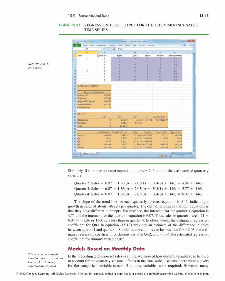
15.5 Seasonality and Trend 15-45
Similarly, if time period t corresponds to quarters 2, 3, and 4, the estimates of quarterlysales are
The slope of the trend line for each quarterly forecast equation is .146, indicating agrowth in sales of about 146 sets per quarter. The only difference in the four equations isthat they have different intercepts. For instance, the intercept for the quarter 1 equation is4.71 and the intercept for the quarter 4 equation is 6.07. Thus, sales in quarter 1 are 4.71 �6.07 � �1.36 or 1360 sets less than in quarter 4. In other words, the estimated regressioncoefficient for Qtr1 in equation (15.12) provides an estimate of the difference in salesbetween quarter 1 and quarter 4. Similar interpretations can be provided for �2.03, the esti-mated regression coefficient for dummy variable Qtr2, and �.304, the estimated regressioncoefficient for dummy variable Qtr3.
Models Based on Monthly DataIn the preceding television set sales example, we showed how dummy variables can be usedto account for the quarterly seasonal effects in the time series. Because there were 4 levelsfor the categorical variable season, 3 dummy variables were required. However, many
Quarter 2: Sales � 6.07 � 1.36(0) � 2.03(1) � .304(0) � .146t � 4.04 � .146t
Quarter 3: Sales � 6.07 � 1.36(0) � 2.03(0) � .304(1) � .146t � 5.77 � .146t
Quarter 4: Sales � 6.07 � 1.36(0) � 2.03(0) � .304(0) � .146t � 6.07 � .146t
FIGURE 15.23 REGRESSION TOOL OUTPUT FOR THE TELEVISION SET SALES TIME SERIES
Note: Rows 6–13are hidden.
Whenever a categoricalvariable such as season hask levels, k � 1 dummyvariables are required.
© 2012 Cengage Learning. All Rights Reserved. May not be scanned, copied or duplicated, or posted to a publicly accessible website, in whole or in part.

15-46 Chapter 15 Time Series Analysis and Forecasting
businesses use monthly rather than quarterly forecasts. For monthly data, season is a cate-gorical variable with 12 levels and thus 12 � 1 � 11 dummy variables are required. For ex-ample, the 11 dummy variables could be coded as follows:
.
.
.
Other than this change, the multiple regression approach for handling seasonality remainsthe same.
Exercises
Methods28. Consider the following time series.
Month11 � �1 if November
0 otherwise
Month2 � �1 if February
0 otherwise
Month1 � �1 if January
0 otherwise
Quarter Year 1 Year 2 Year 3
1 71 68 622 49 41 513 58 60 534 78 81 72
testSELF
Quarter Year 1 Year 2 Year 3
1 4 6 72 2 3 63 3 5 64 5 7 8
a. Construct a time series plot. What type of pattern exists in the data?b. Use the following dummy variables to develop an estimated regression equation to
account for seasonal effects in the data: Qtr1 � 1 if Quarter 1, 0 otherwise; Qtr2 � 1if Quarter 2, 0 otherwise; Qtr3 � 1 if Quarter 3, 0 otherwise.
c. Compute the quarterly forecasts for next year.
29. Consider the following time series data.
a. Construct a time series plot. What type of pattern exists in the data?b. Use the following dummy variables to develop an estimated regression equation to
account for any seasonal and linear trend effects in the data: Qtr1 � 1 if Quarter 1, 0otherwise; Qtr2 � 1 if Quarter 2, 0 otherwise; Qtr3 � 1 if Quarter 3, 0 otherwise.
c. Compute the quarterly forecasts for next year.
© 2012 Cengage Learning. All Rights Reserved. May not be scanned, copied or duplicated, or posted to a publicly accessible website, in whole or in part.

15.5 Seasonality and Trend 15-47
a. Construct a time series plot. What type of pattern exists in the data?b. Use the following dummy variables to develop an estimated regression equation to
account for any seasonal effects in the data: Qtr1 � 1 if Quarter 1, 0 otherwise;Qtr2 � 1 if Quarter 2, 0 otherwise; Qtr3 � 1 if Quarter 3, 0 otherwise.
c. Compute the quarterly forecasts for next year.d. Let t � 1 to refer to the observation in quarter 1 of year 1; t � 2 to refer to the obser-
vation in quarter 2 of year 1; . . . and t � 12 to refer to the observation in quarter 4 ofyear 3. Using the dummy variables defined in part (b) and t, develop an estimated regression equation to account for seasonal effects and any linear trend in the time series. Based upon the seasonal effects in the data and linear trend, compute the quar-terly forecasts for next year.
31. Air pollution control specialists in southern California monitor the amount of ozone, car-bon dioxide, and nitrogen dioxide in the air on an hourly basis. The hourly time series dataexhibit seasonality, with the levels of pollutants showing patterns that vary over the hoursin the day. On July 15, 16, and 17, the following levels of nitrogen dioxide were observedfor the 12 hours from 6:00 A.M. to 6:00 P.M.
July 15: 25 28 35 50 60 60 40 35 30 25 25 20July 16: 28 30 35 48 60 65 50 40 35 25 20 20July 17: 35 42 45 70 72 75 60 45 40 25 25 25
a. Construct a time series plot. What type of pattern exists in the data?b. Use the following dummy variables to develop an estimated regression equation to ac-
count for the seasonal effects in the data.
Hour1 � 1 if the reading was made between 6:00 A.M. and 7:00 A.M.;0 otherwiseHour2 � 1 if if the reading was made between 7:00 A.M. and 8:00 A.M.;0 otherwise...Hour11 � 1 if the reading was made between 4:00 P.M. and 5:00 P.M.;0 otherwise.
Note that when the values of the 11 dummy variables are equal to 0, the observation cor-responds to the 5:00 P.M. to 6:00 P.M. hour.c. Using the estimated regression equation developed in part (a), compute estimates of
the levels of nitrogen dioxide for July 18.d. Let t � 1 to refer to the observation in hour 1 on July 15; t � 2 to refer to the obser-
vation in hour 2 of July 15; . . . and t � 36 to refer to the observation in hour 12 of July 17. Using the dummy variables defined in part (b) and t, develop an estimatedregression equation to account for seasonal effects and any linear trend in the timeseries. Based upon the seasonal effects in the data and linear trend, compute estimatesof the levels of nitrogen dioxide for July 18.
Quarter Year 1 Year 2 Year 3
1 1690 1800 18502 940 900 11003 2625 2900 29304 2500 2360 2615
Applications30. The quarterly sales data (number of copies sold) for a college textbook over the past three
years follow.
fileWEBPollution
© 2012 Cengage Learning. All Rights Reserved. May not be scanned, copied or duplicated, or posted to a publicly accessible website, in whole or in part.

15-48 Chapter 15 Time Series Analysis and Forecasting
Quarter Year 1 Year 2 Year 3 Year 4 Year 5
1 20 37 75 92 1762 100 136 155 202 2823 175 245 326 384 4454 13 26 48 82 181
fileWEBSouthShore
32. South Shore Construction builds permanent docks and seawalls along the southern shoreof Long Island, New York. Although the firm has been in business only five years, rev-enue has increased from $308,000 in the first year of operation to $1,084,000 in the mostrecent year. The following data show the quarterly sales revenue in thousands of dollars.
a. Construct a time series plot. What type of pattern exists in the data?b. Use the following dummy variables to develop an estimated regression equation to
account for seasonal effects in the data. Qtr1 � 1 if Quarter 1, 0 otherwise; Qtr2 � 1if Quarter 2, 0 otherwise; Qtr3 � 1 if Quarter 3, 0 otherwise. Based only on the sea-sonal effects in the data, compute estimates of quarterly sales for year 6.
c. Let Period � 1 to refer to the observation in quarter 1 of year 1; Period = 2 to refer tothe observation in quarter 2 of year 1; . . . and Period � 20 to refer to the observationin quarter 4 of year 5. Using the dummy variables defined in part (b) and Period,develop an estimated regression equation to account for seasonal effects and any lineartrend in the time series. Based upon the seasonal effects in the data and linear trend,compute estimates of quarterly sales for year 6.
33. Electric power consumption is measured in kilowatt-hours (kWh). The local utility com-pany offers an interrupt program whereby commercial customers that participate receivefavorable rates but must agree to cut back consumption if the utility requests them to doso. Timko Products has agreed to cut back consumption from noon to 8:00 P.M. on Thurs-day. To determine Timko’s savings, the utility must estimate Timko’s normal power usagefor this period of time. Data on Timko’s electric power consumption for the previous72 hours are shown below.
Time Period Monday Tuesday Wednesday Thursday
12–4 A.M. — 19,281 31,209 27,3304–8 A.M — 33,195 37,014 32,7158–12 noon — 99,516 119,968 152,46512–4 P.M. 124,299 123,666 156,0334–8 P.M. 113,545 111,717 128,8898–12 midnight 41,300 48,112 73,923
fileWEBPower
a. Construct a time series plot. What type of pattern exists in the data?b. Use the following dummy variables to develop an estimated regression equation to
account for any seasonal effects in the data.
Time1 � 1 for time period 12–4 A.M.; 0 otherwiseTime2 � 1 for time period 4–8 A.M.; 0 otherwiseTime3 � 1 for time period 8–12 noon; 0 otherwiseTime4 � 1 for time period 12–4 P.M.; 0 otherwiseTime5 � 1 for time period 4–8 P.M.; 0 otherwise
c. Use the estimated regression equation developed in part (b) to estimate Timko’s nor-mal usage over the period of interrupted service.
d. Let Period � 1 to refer to the observation for Monday in the time period 12–4 P.M.;Period � 2 to refer to the observation for Monday in the time period 4–8 P.M.; . . . andPeriod � 18 to refer to the observation for Thursday in the time period 8–12 noon. Using
© 2012 Cengage Learning. All Rights Reserved. May not be scanned, copied or duplicated, or posted to a publicly accessible website, in whole or in part.

15.6 Time Series Decomposition 15-49
the dummy variables defined in part (b) and Period, develop an estimated regressionequation to account for seasonal effects and any linear trend in the time series.
e. Using the estimated regression equation developed in part (d), estimate Timko’snormal usage over the period of interrupted service.
34. Three years of monthly lawn-maintenance expenses ($) for a six-unit apartment house insouthern Florida follow.
Month Year 1 Year 2 Year 3
January 170 180 195February 180 205 210March 205 215 230April 230 245 280May 240 265 290June 315 330 390July 360 400 420August 290 335 330September 240 260 290October 240 270 295November 230 255 280December 195 220 250
fileWEBAptExp
a. Construct a time series plot. What type of pattern exists in the data?b. Develop an estimated regression equation that can be used to account for any seasonal
and linear trend effects in the data. Use the following dummy variables to account forthe seasonal effects in the data: Jan � 1 if January, 0 otherwise; Feb � 1 if February,0 otherwise; Mar � 1 if March, 0 otherwise; . . . Nov � 1 if November, 0 otherwise.Note that using this coding method, when all the 11 dummy variables are 0, the ob-servation corresponds to an expense in December.
c. Compute the monthly forecasts for next year based upon both trend and seasonal effects.
Time Series DecompositionIn this section we turn our attention to what is called time series decomposition. Timeseries decomposition can be used to separate or decompose a time series into seasonal,trend, and irregular components. While this method can be used for forecasting, its primaryapplicability is to get a better understanding of the time series. Many business and economictime series are maintained and published by government agencies such as the CensusBureau and the Bureau of Labor Statistics. These agencies use time series decompositionto create deseasonalized time series.
Understanding what is really going on with a time series often depends upon the use ofdeseasonalized data. For instance, we might be interested in learning whether electricalpower consumption is increasing in our area. Suppose we learn that electric powerconsumption in September is down 3% from the previous month. Care must be exercised inusing such information, because whenever a seasonal influence is present, such comparisonsmay be misleading if the data have not been deseasonalized. The fact that electric powerconsumption is down 3% from August to September might be only the seasonal effect asso-ciated with a decrease in the use of air conditioning and not because of a long-term declinein the use of electric power. Indeed, after adjusting for the seasonal effect, we might evenfind that the use of electric power increased. Many other time series, such as unemploymentstatistics, home sales, and retail sales, are subject to strong seasonal influences. It is impor-tant to deseasonalize such data before making a judgment about any long-term trend.
15.6
© 2012 Cengage Learning. All Rights Reserved. May not be scanned, copied or duplicated, or posted to a publicly accessible website, in whole or in part.
15-50 Chapter 15 Time Series Analysis and Forecasting
Time series decomposition methods assume that Yt, the actual time series value atperiod t, is a function of three components: a trend component; a seasonal component; andan irregular or error component. How these three components are combined to generate theobserved values of the time series depends upon whether we assume the relationship is bestdescribed by an additive or a multiplicative model.
An additive decomposition model takes the following form:
(15.9)
where
In an additive model the values for the three components are simply added together to obtain the actual time series value Yt. The irregular or error component accounts for the vari-ability in the time series that cannot be explained by the trend and seasonal components.
An additive model is appropriate in situations where the seasonal fluctuations do notdepend upon the level of the time series. The regression model for incorporating seasonaland trend effects in Section 15.5 is an additive model. If the sizes of the seasonal fluctua-tions in earlier time periods are about the same as the sizes of the seasonal fluctuations inlater time periods, an additive model is appropriate. However, if the seasonal fluctuationschange over time, growing larger as the sales volume increases because of a long-term lin-ear trend, then a multiplicative model should be used. Many business and economic timeseries follow this pattern.
A multiplicative decomposition model takes the following form:
(15.10)
where
In this model, the trend and seasonal and irregular components are multiplied to give thevalue of the time series. Trend is measured in units of the item being forecast. However,the seasonal and irregular components are measured in relative terms, with values above1.00 indicating effects above the trend and values below 1.00 indicating effects belowthe trend.
Because this is the method most often used in practice, we will restrict our discussionof time series decomposition to showing how to develop estimates of the trend and sea-sonal components for a multiplicative model. As an illustration we will work with the quar-terly television set sales time series introduced in Section 15.5; the quarterly sales data areshown in Table 15.18 and the corresponding time series plot is presented in Figure 15.22.After demonstrating how to decompose a time series using the multiplicative model, wewill show how the seasonal indices and trend component can be recombined to develop aforecast.
Calculating the Seasonal IndexesFigure 15.22 indicates that sales are lowest in the second quarter of each year and increasein quarters 3 and 4. Thus, we conclude that a seasonal pattern exists for the television setsales time series. The computational procedure used to identify each quarter’s seasonal
Trendt � trend value at time period t
Seasonalt � seasonal index at time period t
Irregulart � irregular index at time period t
Y t � Trendt � Seasonalt � Irregulart
Trendt � trend value at time period t
Seasonalt � seasonal value at time period t
Irregulart � irregular value at time period t
Y t � Trendt � Seasonalt � Irregulart
The irregular componentcorresponds to the errorterm � in the simple linearregression model wediscussed in Chapter 12.
The Census Bureau uses amultiplicative model inconjunction with itsmethodology fordeseasonalizing time series.
© 2012 Cengage Learning. All Rights Reserved. May not be scanned, copied or duplicated, or posted to a publicly accessible website, in whole or in part.

15.6 Time Series Decomposition 15-51
influence begins by computing a moving average to remove the combined seasonal andirregular effects from the data, leaving us with a time series that contains only trend and anyremaining random variation not removed by the moving average calculations.
Because we are working with a quarterly series, we will use four data values in eachmoving average. The moving average calculation for the first four quarters of the televisionset sales data is
Note that the moving average calculation for the first four quarters yields the average quar-terly sales over year 1 of the time series. Continuing the moving average calculations, wenext add the 5.8 value for the first quarter of year 2 and drop the 4.8 for the first quarter ofyear 1. Thus, the second moving average is
Similarly, the third moving average calculation is (6.0 � 6.5 � 5.8 � 5.2)/4 � 5.875.Before we proceed with the moving average calculations for the entire time series, let
us return to the first moving average calculation, which resulted in a value of 5.35. The5.35 value is the average quarterly sales volume for year 1. As we look back at the calcu-lation of the 5.35 value, associating 5.35 with the “middle” of the moving average groupmakes sense. Note, however, that with four quarters in the moving average, there is no mid-dle period. The 5.35 value really corresponds to period 2.5, the last half of quarter 2 andthe first half of quarter 3. Similarly, if we go to the next moving average value of 5.60, themiddle period corresponds to period 3.5, the last half of quarter 3 and the first half ofquarter 4.
The two moving average values we computed do not correspond directly to the origi-nal quarters of the time series. We can resolve this difficulty by computing the average ofthe two moving averages. Since the center of the first moving average is period 2.5 (half aperiod or quarter early) and the center of the second moving average is period 3.5 (half aperiod or quarter late), the average of the two moving averages is centered at quarter 3,exactly where it should be. This moving average is referred to as a centered moving average.Thus, the centered moving average for period 3 is (5.35 � 5.60)/2 � 5.475. Similarly, thecentered moving average value for period 4 is (5.60 � 5.875)/2 � 5.738. Table 15.20 showsa complete summary of the moving average and centered moving average calculations forthe television set sales data.
What do the centered moving averages in Table 15.20 tell us about this time series?Figure 15.24 shows a time series plot of the actual time series values and the centered mov-ing average values. Note particularly how the centered moving average values tend to“smooth out” both the seasonal and irregular fluctuations in the time series. The centeredmoving averages represent the trend in the data and any random variation that was not removed by using moving averages to smooth the data.
Previously we showed that the multiplicative decomposition model is
By dividing each side of this equation by the trend component Tt, we can identify the com-bined seasonal-irregular effect in the time series.
Yt � Trendt � Seasonalt � Irregulart
Second moving average �4.1 � 6.0 � 6.5 � 5.8
4�
22.4
4� 5.60
First moving average �4.8 � 4.1 � 6.0 � 6.5
4�
21.4
4� 5.35
© 2012 Cengage Learning. All Rights Reserved. May not be scanned, copied or duplicated, or posted to a publicly accessible website, in whole or in part.
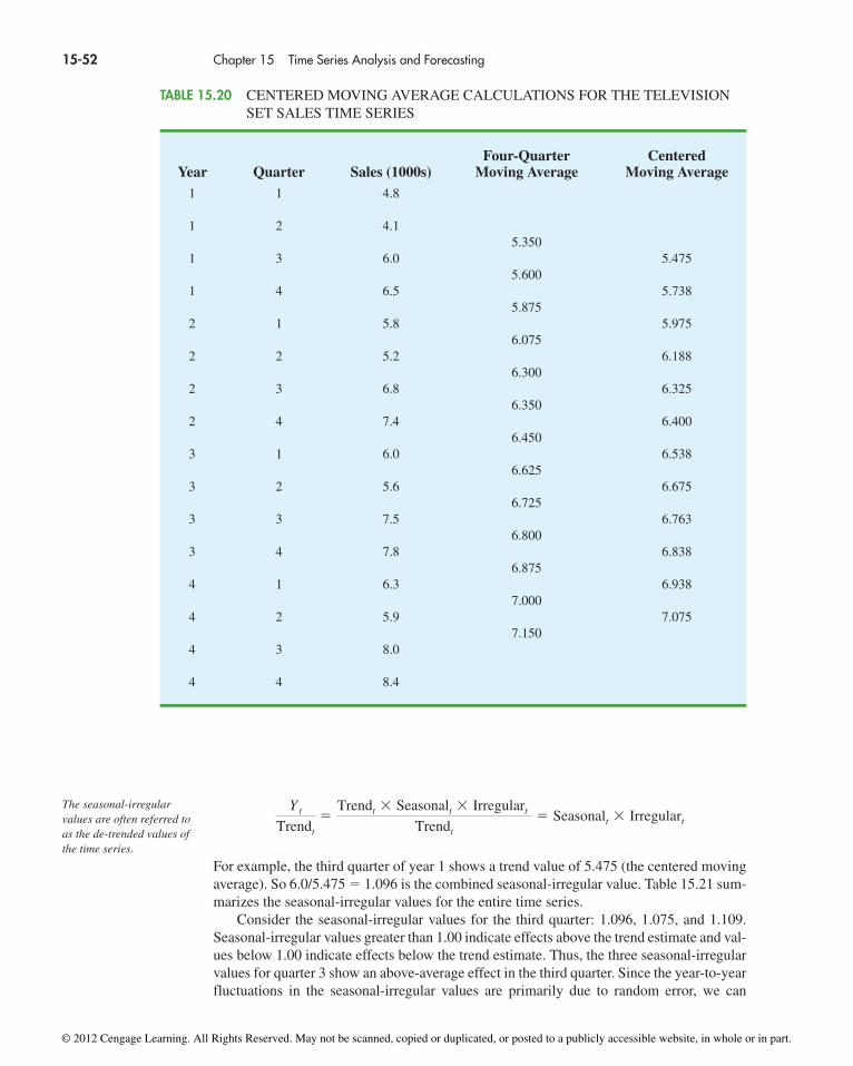
For example, the third quarter of year 1 shows a trend value of 5.475 (the centered movingaverage). So 6.0/5.475 � 1.096 is the combined seasonal-irregular value. Table 15.21 sum-marizes the seasonal-irregular values for the entire time series.
Consider the seasonal-irregular values for the third quarter: 1.096, 1.075, and 1.109.Seasonal-irregular values greater than 1.00 indicate effects above the trend estimate and val-ues below 1.00 indicate effects below the trend estimate. Thus, the three seasonal-irregularvalues for quarter 3 show an above-average effect in the third quarter. Since the year-to-yearfluctuations in the seasonal-irregular values are primarily due to random error, we can
Yt
Trendt
�Trendt � Seasonalt � Irregulart
Trendt
� Seasonalt � Irregulart
15-52 Chapter 15 Time Series Analysis and Forecasting
The seasonal-irregularvalues are often referred toas the de-trended values ofthe time series.
Four-Quarter CenteredYear Quarter Sales (1000s) Moving Average Moving Average
1 1 4.8
1 2 4.15.350
1 3 6.0 5.4755.600
1 4 6.5 5.7385.875
2 1 5.8 5.9756.075
2 2 5.2 6.1886.300
2 3 6.8 6.3256.350
2 4 7.4 6.4006.450
3 1 6.0 6.5386.625
3 2 5.6 6.6756.725
3 3 7.5 6.7636.800
3 4 7.8 6.8386.875
4 1 6.3 6.9387.000
4 2 5.9 7.0757.150
4 3 8.0
4 4 8.4
TABLE 15.20 CENTERED MOVING AVERAGE CALCULATIONS FOR THE TELEVISIONSET SALES TIME SERIES
© 2012 Cengage Learning. All Rights Reserved. May not be scanned, copied or duplicated, or posted to a publicly accessible website, in whole or in part.

15.6 Time Series Decomposition 15-53
Qua
rter
ly T
elev
isio
n Se
t Sa
les
(100
0s)
9.0
4 3 1 2 3 4 1 2 3 41 2 3 21 4
7.0
8.0
6.0
5.0
4.0
3.0
2.0
1.0
0.0
Centeredmoving average
time series
Year 1 Year 2 Year 3 Year 4
Year/Quarter
FIGURE 15.24 QUARTERLY TELEVISION SET SALES TIME SERIES AND CENTEREDMOVING AVERAGE
Centered Seasonal-IrregularYear Quarter Sales (1000s) Moving Average Value
1 1 4.81 2 4.11 3 6.0 5.475 1.0961 4 6.5 5.738 1.1332 1 5.8 5.975 0.9712 2 5.2 6.188 0.8402 3 6.8 6.325 1.0752 4 7.4 6.400 1.1563 1 6.0 6.538 0.9183 2 5.6 6.675 0.8393 3 7.5 6.763 1.1093 4 7.8 6.838 1.1414 1 6.3 6.938 0.9084 2 5.9 7.075 0.8344 3 8.04 4 8.4
TABLE 15.21 SEASONAL IRREGULAR VALUES FOR THE TELEVISION SET SALES TIME SERIES
© 2012 Cengage Learning. All Rights Reserved. May not be scanned, copied or duplicated, or posted to a publicly accessible website, in whole or in part.

average the computed values to eliminate the irregular influence and obtain an estimate ofthe third-quarter seasonal influence.
We refer to 1.09 as the seasonal index for the third quarter. Table 15.22 summarizes thecalculations involved in computing the seasonal indexes for the television set sales timeseries. The seasonal indexes for the four quarters are .93, .84, 1.09, and 1.14.
Interpretation of the seasonal indexes in Table 15.22 provides some insight about theseasonal component in television set sales. The best sales quarter is the fourth quarter, withsales averaging 14% above the trend estimate. The worst, or slowest, sales quarter is thesecond quarter; its seasonal index of .84 shows that the sales average is 16% below thetrend estimate. The seasonal component corresponds clearly to the intuitive expectationthat television viewing interest and thus television purchase patterns tend to peak in thefourth quarter because of the coming winter season and reduction in outdoor activities. Thelow second-quarter sales reflect the reduced interest in television viewing due to the springand presummer activities of potential customers.
One final adjustment is sometimes necessary in obtaining the seasonal indexes. Be-cause the multiplicative model requires that the average seasonal index equal 1.00, the sumof the four seasonal indexes in Table 15.22 must equal 4.00. In other words, the seasonaleffects must even out over the year. The average of the seasonal indexes in our example isequal to 1.00, and hence this type of adjustment is not necessary. In other cases, a slightadjustment may be necessary. To make the adjustment, multiply each seasonal index bythe number of seasons divided by the sum of the unadjusted seasonal indexes. For instance,for quarterly data, multiply each seasonal index by 4/(sum of the unadjusted seasonalindexes). Some of the exercises will require this adjustment to obtain the appropriateseasonal indexes.
Deseasonalizing the Time SeriesA time series that has had the seasonal effects removed is referred to as a deseasonalizedtime series, and the process of using the seasonal indexes to remove the seasonal effectsfrom a time series is referred to as deseasonalizing the time series. Using a multiplicativedecomposition model, we deseasonalize a time series by dividing each observation by itscorresponding seasonal index. The multiplicative decomposition model is
So, when we divide each time series observation (Yt) by its corresponding seasonal index,the resulting data show only trend and random variability (the irregular component). The
Yt � Trendt � Seasonalt � Irregulart
Seasonal effect of quarter 3 �1.096 � 1.075 � 1.109
3� 1.09
15-54 Chapter 15 Time Series Analysis and Forecasting
Quarter Seasonal-Irregular Values Seasonal Index1 0.971 0.918 0.908 0.932 0.840 0.839 0.834 0.843 1.096 1.075 1.109 1.094 1.133 1.156 1.141 1.14
TABLE 15.22 SEASONAL INDEX CALCULATIONS FOR THE TELEVISION SET SALES TIME SERIES
Economic time seriesadjusted for seasonalvariations are oftenreported in publicationssuch as the Survey ofCurrent Business, The WallStreet Journal, andBloomberg Businessweek.
© 2012 Cengage Learning. All Rights Reserved. May not be scanned, copied or duplicated, or posted to a publicly accessible website, in whole or in part.

15.6 Time Series Decomposition 15-55
deseasonalized time series for television set sales is summarized in Table 15.23. A graph ofthe deseasonalized time series is shown in Figure 15.25.
Using the Deseasonalized Time Series to Identify TrendThe graph of the deseasonalized television set sales time series shown in Figure 15.25appears to have an upward linear trend. To identify this trend, we will fit a linear trend
Time Sales Seasonal Deseasonalized Year Quarter Period (1000s) Index Sales
1 1 1 4.8 0.93 5.162 2 4.1 0.84 4.883 3 6.0 1.09 5.504 4 6.5 1.14 5.70
2 1 5 5.8 0.93 6.242 6 5.2 0.84 6.193 7 6.8 1.09 6.244 8 7.4 1.14 6.49
3 1 9 6.0 0.93 6.452 10 5.6 0.84 6.673 11 7.5 1.09 6.884 12 7.8 1.14 6.84
4 1 13 6.3 0.93 6.772 14 5.9 0.84 7.023 15 8.0 1.09 7.344 16 8.4 1.14 7.37
TABLE 15.23 DESEASONALIZED VALUES FOR THE TELEVISION SET SALES TIME SERIES
Des
easo
naliz
ed S
ales
(10
00s)
8.0
4 3 1 2 3 4 1 2 3 41 2 3 21 4
7.0
6.0
5.0
4.0
3.0
2.0
1.0
0.0
Year 1 Year 2 Year 3 Year 4
FIGURE 15.25 DESEASONALIZED TELEVISION SET SALES TIME SERIES
© 2012 Cengage Learning. All Rights Reserved. May not be scanned, copied or duplicated, or posted to a publicly accessible website, in whole or in part.

equation to the deseasonalized time series using the same method shown in Section 15.4.The only difference is that we will be fitting a trend line to the deseasonalized data insteadof the original data.
Recall that for a linear trend the estimated regression equation can be written as
where
In Section 15.4 we provided formulas for computing the values of b0 and b1. To fit a lineartrend line to the deseasonalized data in Table 15.23, the only change is that the deseasonal-ized time series values are used instead of the observed values Yt in computing b0 and b1.Using Excel’s Regression tool, the estimated linear trend equation is
The slope of 0.148 indicates that over the past 16 quarters, the firm averaged a desea-sonalized growth in sales of about 148 sets per quarter. If we assume that the past 16-quartertrend in sales data is a reasonably good indicator of the future, this equation can be used todevelop a trend projection for future quarters. For example, substituting t � 17 into theequation yields next quarter’s deseasonalized trend projection, T17.
Thus, using the deseasonalized data, the linear trend forecast for next quarter (period 17) is7616 television sets. Similarly, the deseasonalized trend forecasts for the next three quar-ters (periods 18, 19, and 20) are 7764, 7912, and 8060 television sets, respectively.
Seasonal AdjustmentsThe final step in developing the forecast when both trend and seasonal components are pres-ent is to use the seasonal indexes to adjust the deseasonalized trend projections. Returningto the television set sales example, we have a deseasonalized trend projection for the nextfour quarters. Now we must adjust the forecast for the seasonal effect. The seasonal indexfor the first quarter of year 5 (t � 17) is 0.93, so we obtain the quarterly forecast by multi-plying the deseasonalized forecast based on trend (T17 � 7616) by the seasonal index (0.93).Thus, the forecast for the next quarter is 7616(0.93) � 7083. Table 15.24 shows the quar-terly forecast for quarters 17 through 20. The high-volume fourth quarter has a 9188-unitforecast, and the low-volume second quarter has a 6522-unit forecast.
Models Based on Monthly DataIn the preceding television set sales example, we used quarterly data to illustrate the com-putation of seasonal indexes. However, many businesses use monthly rather than quarterlyforecasts. In such cases, the procedures introduced in this section can be applied with
T17 � 5.10 � 0.148(17) � 7.616
Deseasonalized Sales � 5.10 � 0.148t
Tt � linear trend forecast in period t
b0 � intercept of the linear trend line
b1 � slope of the trend line
t � time period
Tt � b0 � b1t
15-56 Chapter 15 Time Series Analysis and Forecasting
© 2012 Cengage Learning. All Rights Reserved. May not be scanned, copied or duplicated, or posted to a publicly accessible website, in whole or in part.

15.6 Time Series Decomposition 15-57
minor modifications. First, a 12-month moving average replaces the four-quarter movingaverage; second, 12 monthly seasonal indexes, rather than four quarterly seasonal indexes,must be computed. Other than these changes, the computational and forecasting proceduresare identical.
Cyclical ComponentMathematically, the multiplicative model of equation (15.14) can be expanded to include acyclical component.
(15.11)
The cyclical component, like the seasonal component, is expressed as a percentage of trend.As mentioned in Section 15.1, this component is attributable to multiyear cycles in the timeseries. It is analogous to the seasonal component, but over a longer period of time. How-ever, because of the length of time involved, obtaining enough relevant data to estimate thecyclical component is often difficult. Another difficulty is that cycles usually vary in length.Because it is so difficult to identify and/or separate cyclical effects from long-term trend effects, in practice these effects are often combined and referred to as a combined trend-cycle component. We leave further discussion of the cyclical component to specialized textson forecasting methods.
Yt � Trendt � Cyclicalt � Seasonalt � Irregulart
DeseasonalizedYear Quarter Trend Forecast Seasonal Index Quarterly Forecast
5 1 7616 0.93 (7616)(0.93) � 70832 7764 0.84 (7764)(0.84) � 65223 7912 1.09 (7912)(1.09) � 86244 8060 1.14 (8060)(1.14) � 9188
TABLE 15.24 QUARTERLY FORECASTS FOR THE TELEVISION SET SALES TIME SERIES
NOTES AND COMMENTS
1. There are a number of different approaches tocomputing the seasonal indexes. In this sectioneach seasonal index was computed by averag-ing the corresponding seasonal-irregular val-ues. Another approach is to use the median ofthe seasonal-irregular values as the seasonalindex.
2. Calendar adjustments are often made before de-seasonalizing a time series. For example, if atime series consists of monthly sales values, thevalue for February sales may be less than for
another month simply because there are fewerdays in February. To account for this factor, wewould first divide each month’s sales value bythe number of days in the month to obtain adaily average. Since the average number of daysin a month is approximately 365/12 � 30.4167,we then multiply the daily averages by 30.4167to obtain adjusted monthly values. For theexamples and exercises in this chapter, you canassume that any required calendar adjustmentshave already been made.
© 2012 Cengage Learning. All Rights Reserved. May not be scanned, copied or duplicated, or posted to a publicly accessible website, in whole or in part.

Exercises
Methods35. Consider the following time series data.
15-58 Chapter 15 Time Series Analysis and Forecasting
Quarter Year 1 Year 2 Year 3
1 4 6 72 2 3 63 3 5 64 5 7 8
testSELF
Quarter Year 1 Year 2 Year 3
1 1690 1800 18502 940 900 11003 2625 2900 29304 2500 2360 2615
fileWEBTextSales
a. Construct a time series plot. What type of pattern exists in the data?b. Show the four-quarter and centered moving average values for this time series.c. Compute seasonal indexes and adjusted seasonal indexes for the four quarters.
36. Refer to exercise 35. a. Deseasonalize the time series using the adjusted seasonal indexes computed in part (c)
of exercise 35.b. Compute the linear trend regression equation for the deseasonalized data.c. Compute the deseasonalized quarterly trend forecast for Year 4.d. Use the seasonal indexes to adjust the deseasonalized trend forecasts computed in
part (c).
Applications37. The quarterly sales data (number of copies sold) for a college textbook over the past three
years follow.
a. Construct a time series plot. What type of pattern exists in the data?b. Show the four-quarter and centered moving average values for this time series.c. Compute the seasonal and adjusted seasonal indexes for the four quarters.d. When does the publisher have the largest seasonal index? Does this result appear rea-
sonable? Explain.e. Deseasonalize the time series.f. Compute the linear trend equation for the deseasonalized data and forecast sales
using the linear trend equation.g. Adjust the linear trend forecasts using the adjusted seasonal indexes computed in
part (c).
© 2012 Cengage Learning. All Rights Reserved. May not be scanned, copied or duplicated, or posted to a publicly accessible website, in whole or in part.

15.6 Time Series Decomposition 15-59
38. Three years of monthly lawn-maintenance expenses ($) for a six-unit apartment house insouthern Florida follow.
Month Year 1 Year 2 Year 3
January 170 180 195February 180 205 210March 205 215 230April 230 245 280May 240 265 290June 315 330 390July 360 400 420August 290 335 330September 240 260 290October 240 270 295November 230 255 280December 195 220 250
fileWEBAptExp
fileWEBPollution
a. Construct a time series plot. What type of pattern exists in the data?b. Identify the monthly seasonal indexes for the three years of lawn-maintenance
expenses for the apartment house in southern Florida as given here. Use a 12-monthmoving average calculation.
c. Deseasonalize the time series.d. Compute the linear trend equation for the deseasonalized data. e. Compute the deseasonalized trend forecasts and then adjust the trend forecasts using
the seasonal indexes to provide a forecast for monthly expenses in year 4.
39. Air pollution control specialists in southern California monitor the amount of ozone,carbon dioxide, and nitrogen dioxide in the air on an hourly basis. The hourly time seriesdata exhibit seasonality, with the levels of pollutants showing patterns over the hours in theday. On July 15, 16, and 17, the following levels of nitrogen dioxide were observed in thedowntown area for the 12 hours from 6:00 A.M. to 6:00 P.M.
July 15: 25 28 35 50 60 60 40 35 30 25 25 20
July 16: 28 30 35 48 60 65 50 40 35 25 20 20
July 17: 35 42 45 70 72 75 60 45 40 25 25 25
a. Construct a time series plot. What type of pattern exists in the data?b. Identify the hourly seasonal indexes for the 12 readings each day.c. Deseasonalize the time series.d. Compute the linear trend equation for the deseasonalized data. e. Compute the deseasonalized trend forecasts for the 12 hours for July 18 and then
adjust the trend forecasts using the seasonal indexes computed in part (b).
40. Electric power consumption is measured in kilowatt-hours (kWh). The local utility com-pany offers an interrupt program whereby commercial customers that participate receivefavorable rates but must agree to cut back consumption if the utility requests them to doso. Timko Products cut back consumption at 12:00 noon Thursday. To assess the savings,the utility must estimate Timko’s usage without the interrupt. The period of interruptedservice was from noon to 8:00 P.M. Data on electric power consumption for the previous72 hours are available.
© 2012 Cengage Learning. All Rights Reserved. May not be scanned, copied or duplicated, or posted to a publicly accessible website, in whole or in part.
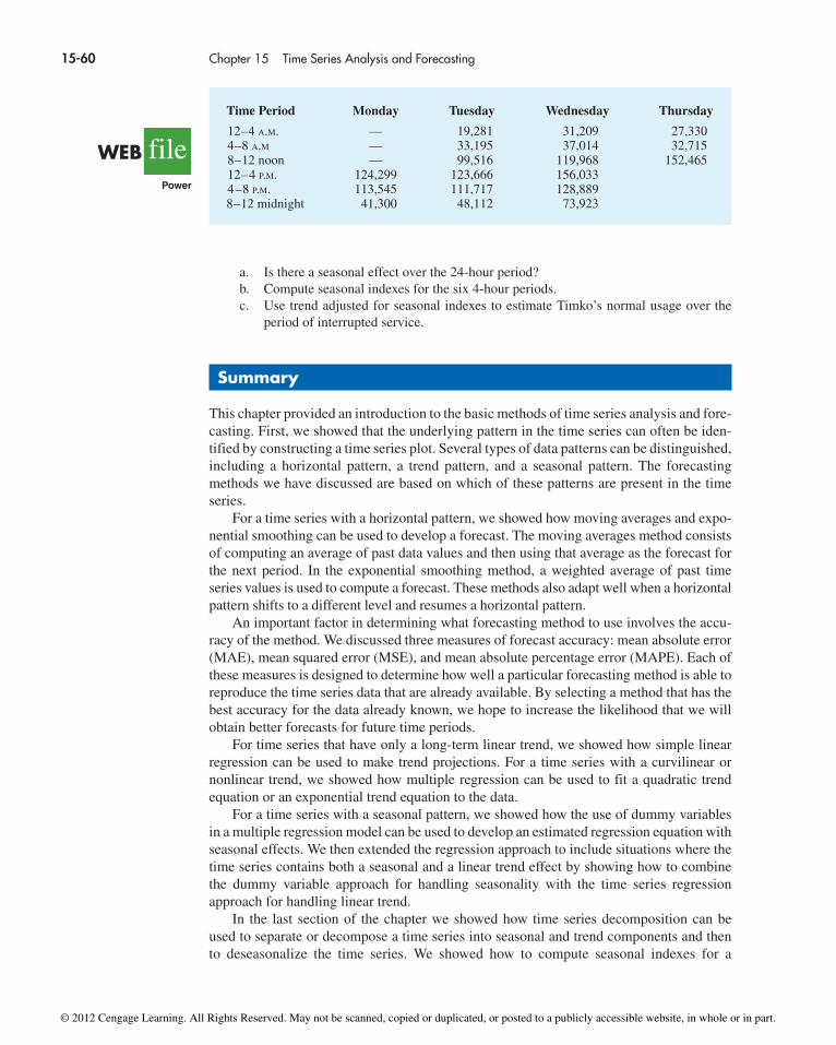
a. Is there a seasonal effect over the 24-hour period? b. Compute seasonal indexes for the six 4-hour periods.c. Use trend adjusted for seasonal indexes to estimate Timko’s normal usage over the
period of interrupted service.
Summary
This chapter provided an introduction to the basic methods of time series analysis and fore-casting. First, we showed that the underlying pattern in the time series can often be iden-tified by constructing a time series plot. Several types of data patterns can be distinguished, including a horizontal pattern, a trend pattern, and a seasonal pattern. The forecastingmethods we have discussed are based on which of these patterns are present in the timeseries.
For a time series with a horizontal pattern, we showed how moving averages and expo-nential smoothing can be used to develop a forecast. The moving averages method consistsof computing an average of past data values and then using that average as the forecast forthe next period. In the exponential smoothing method, a weighted average of past time series values is used to compute a forecast. These methods also adapt well when a horizontalpattern shifts to a different level and resumes a horizontal pattern.
An important factor in determining what forecasting method to use involves the accu-racy of the method. We discussed three measures of forecast accuracy: mean absolute error(MAE), mean squared error (MSE), and mean absolute percentage error (MAPE). Each ofthese measures is designed to determine how well a particular forecasting method is able toreproduce the time series data that are already available. By selecting a method that has thebest accuracy for the data already known, we hope to increase the likelihood that we willobtain better forecasts for future time periods.
For time series that have only a long-term linear trend, we showed how simple linearregression can be used to make trend projections. For a time series with a curvilinear ornonlinear trend, we showed how multiple regression can be used to fit a quadratic trendequation or an exponential trend equation to the data.
For a time series with a seasonal pattern, we showed how the use of dummy variablesin a multiple regression model can be used to develop an estimated regression equation withseasonal effects. We then extended the regression approach to include situations where thetime series contains both a seasonal and a linear trend effect by showing how to combinethe dummy variable approach for handling seasonality with the time series regressionapproach for handling linear trend.
In the last section of the chapter we showed how time series decomposition can beused to separate or decompose a time series into seasonal and trend components and thento deseasonalize the time series. We showed how to compute seasonal indexes for a
15-60 Chapter 15 Time Series Analysis and Forecasting
Time Period Monday Tuesday Wednesday Thursday
12–4 A.M. — 19,281 31,209 27,3304–8 A.M — 33,195 37,014 32,7158–12 noon — 99,516 119,968 152,46512–4 P.M. 124,299 123,666 156,0334–8 P.M. 113,545 111,717 128,8898–12 midnight 41,300 48,112 73,923
fileWEBPower
© 2012 Cengage Learning. All Rights Reserved. May not be scanned, copied or duplicated, or posted to a publicly accessible website, in whole or in part.

Glossary 15-61
multiplicative model, how to use the seasonal indexes to deseasonalize the time series, andhow to use regression analysis on the deseasonalized data to estimate the trend component.The final step in developing a forecast when both trend and seasonal components are present is to use the seasonal indexes to adjust the trend projections.
Glossary
Time series A sequence of observations on a variable measured at successive points in timeor over successive periods of time.Time series plot A graphical presentation of the relationship between time and the timeseries variable. Time is shown on the horizontal axis and the time series values are shownon the verical axis.Horizontal pattern A horizontal pattern exists when the data fluctuate around a constantmean.Stationary time series A time series whose statistical properties are independent of time.For a stationary time series the process generating the data has a constant mean and the vari-ability of the time series is constant over time.Trend pattern A trend pattern exists if the time series plot shows gradual shifts or move-ments to relatively higher or lower values over a longer period of time.Seasonal pattern A seasonal pattern exists if the time series plot exhibits a repeating pat-tern over successive periods. The successive periods are often one-year intervals, which iswhere the name seasonal pattern comes from.Cyclical pattern A cyclical pattern exists if the time series plot shows an alternatingsequence of points below and above the trend line lasting more than one year.Forecast error The difference between the actual time series value and the forecast.Mean absolute error (MAE) The average of the absolute values of the forecast errors.Mean squared error (MSE) The average of the sum of squared forecast errors.Mean absolute percentage error (MAPE) The average of the absolute values of the per-centage forecast errors.Moving averages A forecasting method that uses the average of the most recent k data val-ues in the time series as the forecast for the next period.Weighted moving averages A forecasting method that involves selecting a different weightfor the most recent k data values values in the time series and then computing a weightedaverage of the values. The sum of the weights must equal one.Exponential smoothing A forecasting method that uses a weighted average of past timeseries values as the forecast; it is a special case of the weighted moving averages method inwhich we select only one weight—the weight for the most recent observation.Smoothing constant A parameter of the exponential smoothing model that provides theweight given to the most recent time series value in the calculation of the forecast value.Time series decompostition A time series method that is used to separate or decompose atime series into seasonal and trend components.Additive model In an additive model the actual time series value at time period t is ob-tained by adding the values of a trend component, a seasonal component, and an irregularcomponent.Multiplicative model In a multiplicative model the actual time series value at time periodt is obtained by multiplying the values of a trend component, a seasonal component, and anirregular component.Deseasonalized time series A time series from which the effect of season has been removedby dividing each original time series observation by the corresponding seasonal index.
© 2012 Cengage Learning. All Rights Reserved. May not be scanned, copied or duplicated, or posted to a publicly accessible website, in whole or in part.
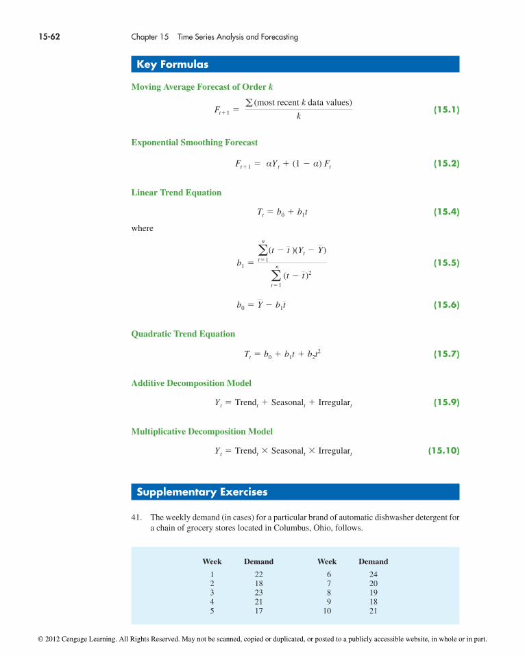
Key Formulas
Moving Average Forecast of Order k
(15.1)
Exponential Smoothing Forecast
(15.2)
Linear Trend Equation
(15.4)
where
(15.5)
(15.6)
Quadratic Trend Equation
(15.7)
Additive Decomposition Model
(15.9)
Multiplicative Decomposition Model
(15.10)
Supplementary Exercises
41. The weekly demand (in cases) for a particular brand of automatic dishwasher detergent fora chain of grocery stores located in Columbus, Ohio, follows.
Yt � Trendt � Seasonalt � Irregulart
Yt � Trendt � Seasonalt � Irregulart
Tt � b0 � b1t � b2t2
b0 � Y � b1t
b1 ��
n
t�1
(t � t )(Yt � Y )
�n
t�1
(t � t )2
Tt � b0 � b1t
Ft�1 � αYt � (1 � α) Ft
Ft�1 �� (most recent k data values)
k
15-62 Chapter 15 Time Series Analysis and Forecasting
Week Demand Week Demand
1 22 6 242 18 7 203 23 8 194 21 9 185 17 10 21
© 2012 Cengage Learning. All Rights Reserved. May not be scanned, copied or duplicated, or posted to a publicly accessible website, in whole or in part.

Supplementary Exercises 15-63
a. Construct a time series plot. What type of pattern exists in the data?b. Use a three-week moving average to develop a forecast for week 11.c. Use exponential smoothing with a smoothing constant of α � .2 to develop a forecast
for week 11.d. Which of the two methods do you prefer? Why?
42. The following table reports the percentage of stocks in a portfolio for nine quarters from2007 to 2009.
Quarter Stock %
1st—2007 29.82nd—2007 31.03rd—2007 29.94th—2007 30.11st—2008 32.2
2nd—2008 31.53rd—2008 32.04th—2008 31.91st—2009 30.0
Week Sales Week Sales
1 2750 7 33002 3100 8 31003 3250 9 29504 2800 10 30005 2900 11 32006 3050 12 3150
a. Construct a time series plot. What type of pattern exists in the data?b. Use exponential smoothing to forecast this time series. Consider smoothing constants
of α � .2, .3, and .4. What value of the smoothing constant provides the most accu-rate forecasts?
c. What is the forecast of the percentage of stocks in a typical portfolio for the secondquarter of 2009?
43. United Dairies, Inc., supplies milk to several independent grocers throughout DadeCounty, Florida. Managers at United Dairies want to develop a forecast of the number ofhalf-gallons of milk sold per week. Sales data for the past 12 weeks follow.
a. Construct a time series plot. What type of pattern exists in the data?b. Use exponential smoothing withf α � .4 to develop a forecast of demand for week 13.
44. To avoid a monthly service fee in an interest-bearing checking account, customers mustmaintain a minimum average daily balance. Bankrate’s 2008 survey of 249 banks andthrifts in the top 25 metropolitan areas showed that you need to maintain an average bal-ance of $3462 to avoid a monthly service fee. With an average fee of $11.97 and an aver-age interest rate of only 0.24 percent, customers with interest-bearing checking accountsare not getting much value for basically providing the bank with a line of credit equal tothe average monthly balance required to avoid the monthly service fee (Bankrate website,October 27, 2008). The following table shows the minimum average balance required toavoid paying a monthly service fee from 2001 to 2008.
© 2012 Cengage Learning. All Rights Reserved. May not be scanned, copied or duplicated, or posted to a publicly accessible website, in whole or in part.

a. Construct a time series plot. What type of pattern exists in the data?b. Compute the linear trend equation for the time series. Compute an estimate of the
average balance required to avoid a monthly service fee for 2009.c. Compute the quadratic trend equation for the time series. Compute an estimate of the
average balance required to avoid a monthly service fee for 2009.d. Using MSE, which approach provides the most accurate forecasts for the historical
data?e. For these data would you recommend that the forecast for 2009 be developed using
the linear trend equation or the quadratic trend equation? Explain.
45. The Garden Avenue Seven sells CDs of its musical performances. The following tablereports sales (in units) for the past 18 months. The group’s manager wants an accuratemethod for forecasting future sales.
15-64 Chapter 15 Time Series Analysis and Forecasting
Year Balance ($)
2001 24352002 25932003 22582004 20872005 22942006 26602007 33172008 3462
Month Sales Month Sales Month Sales
1 293 7 381 13 5492 283 8 431 14 5443 322 9 424 15 6014 355 10 433 16 5875 346 11 470 17 6446 379 12 481 18 660
fileWEBCDSales
a. Construct a time series plot. What type of pattern exists in the data?b. Use exponential smoothing with α � .3, .4, and .5. Which value of α provides the
most accurate forecasts?c. Use trend projection to provide a forecast. What is the value of MSE?d. Which method of forecasting would you recommend to the manager? Why?
46. The Mayfair Department Store in Davenport, Iowa, is trying to determine the amount ofsales lost while it was shut down during July and August because of damage caused by theMississippi River flood. Sales data for January through June follow.
Month Sales ($1000s) Month Sales ($1000s)
January 185.72 April 210.36February 167.84 May 255.57March 205.11 June 261.19
© 2012 Cengage Learning. All Rights Reserved. May not be scanned, copied or duplicated, or posted to a publicly accessible website, in whole or in part.

Supplementary Exercises 15-65
a. Use exponential smoothing, with α � .4, to develop a forecast for July and August.(Hint: Use the forecast for July as the actual sales in July in developing the Augustforecast.) Comment on the use of exponential smoothing for forecasts more than oneperiod into the future.
b. Use trend projection to forecast sales for July and August.c. Mayfair’s insurance company proposed a settlement based on lost sales of $240,000
in July and August. Is this amount fair? If not, what amount would you recommendas a counteroffer?
47. Canton Supplies, Inc., is a service firm that employs approximately 100 individuals.Managers of Canton Supplies are concerned about meeting monthly cash obligations and wantto develop a forecast of monthly cash requirements. Because of a recent change in operatingpolicy, only the past seven months of data that follow are considered to be relevant.
Month 1 2 3 4 5 6 7
Cash Required ($1000s) 205 212 218 224 230 240 246
a. Construct a time series plot. What type of pattern exists in the data?b. Compute the linear trend equation to forecast cash requirements for each of the next
two months.
48. The Costello Music Company has been in business for five years. During that time, salesof pianos increased from 12 units in the first year to 76 units in the most recent year. FredCostello, the firm’s owner, wants to develop a forecast of piano sales for the coming year.The historical data follow.
Year 1 2 3 4 5
Sales 12 28 34 50 76
a. Construct a time series plot. What type of pattern exists in the data?b. Develop the linear trend equation for the time series. What is the average increase in
sales that the firm has been realizing per year?c. Forecast sales for years 6 and 7.
49. Consider the Costello Music Company problem in exercise 48. The quarterly sales datafollow.
Total YearlyYear Quarter 1 Quarter 2 Quarter 3 Quarter 4 Sales
1 4 2 1 5 122 6 4 4 14 283 10 3 5 16 344 12 9 7 22 505 18 10 13 35 76
fileWEBPianoSales
a. Use the following dummy variables to develop an estimated regression equation to account for any seasonal and linear trend effects in the data: Qtr1 � 1 if Quarter 1, 0otherwise; Qtr2 � 1 if Quarter 2, 0 otherwise; and Qtr3 � 1 if Quarter 3, 0 otherwise.
b. Compute the quarterly forecasts for next year.
50. Refer to the Costello Music Company problem in exercise 49. a. Using time series decomposition, compute the seasonal indexes for the four quarters.b. When does Costello Music experience the largest seasonal effect? Does this result
appear reasonable? Explain.
© 2012 Cengage Learning. All Rights Reserved. May not be scanned, copied or duplicated, or posted to a publicly accessible website, in whole or in part.

51. Refer to the Costello Music Company time series in exercise 49.a. Deseasonalize the data and use the deseasonalized time series to identify the trend.b. Use the results of part (a) to develop a quarterly forecast for next year based on trend.c. Use the seasonal indexes developed in exercise 50 to adjust the forecasts developed in
part (b) to account for the effect of season.
52. Hudson Marine has been an authorized dealer for C&D marine radios for the past sevenyears. The following table reports the number of radios sold each year.
Year 1 2 3 4 5 6 7
Number Sold 35 50 75 90 105 110 130
a. Construct a time series plot. Does a linear trend appear to be present?b. Compute the linear trend equation for this time series.c. Use the linear trend equation developed in part (b) to develop a forecast for annual
sales in year 8.
53. Refer to the Hudson Marine problem in exercise 52. Suppose the quarterly sales values forthe seven years of historical data are as follows.
15-66 Chapter 15 Time Series Analysis and Forecasting
Total YearlyYear Quarter 1 Quarter 2 Quarter 3 Quarter 4 Sales
1 6 15 10 4 352 10 18 15 7 503 14 26 23 12 754 19 28 25 18 905 22 34 28 21 1056 24 36 30 20 1107 28 40 35 27 130
fileWEBHudsonMarine
a. Use the following dummy variables to develop an estimated regression equation toaccount for any season and linear trend effects in the data: Qtr1 � 1 if Quarter 1, 0otherwise; Qtr2 � 1 if Quarter 2, 0 otherwise; and Qtr3 � 1 if Quarter 3, 0 otherwise.
b. Compute the quarterly forecasts for next year.
54. Refer to the Hudson Marine problem in exercise 53. a. Compute the centered moving average values for this time series.b. Construct a time series plot that also shows the centered moving average and original
time series on the same graph. Discuss the differences between the original time series plot and the centered moving average time series.
c. Compute the seasonal indexes for the four quarters.d. When does Hudson Marine experience the largest seasonal effect? Does this result
seem reasonable? Explain.
55. Refer to the Hudson Marine data in exercise 53.a. Deseasonalize the data and use the deseasonalized time series to identify the trend.b. Use the results of part (a) to develop a quarterly forecast for next year based on trend.c. Use the seasonal indexes developed in exercise 54 to adjust the forecasts developed in
part (b) to account for the effect of season.
Case Problem 1 Forecasting Food and Beverage SalesThe Vintage Restaurant, on Captiva Island near Fort Myers, Florida, is owned and operatedby Karen Payne. The restaurant just completed its third year of operation. Since openingher restaurant, Karen has sought to establish a reputation for the Vintage as a high-quality
© 2012 Cengage Learning. All Rights Reserved. May not be scanned, copied or duplicated, or posted to a publicly accessible website, in whole or in part.

Case Problem 2 Forecasting Lost Sales 15-67
dining establishment that specializes in fresh seafood. Through the efforts of Karen and herstaff, her restaurant has become one of the best and fastest growing restaurants on the island.
To better plan for future growth of the restaurant, Karen needs to develop a system thatwill enable her to forecast food and beverage sales by month for up to one year in advance.Table 15.25 shows the value of food and beverage sales ($1000s) for the first three years ofoperation.
Managerial ReportPerform an analysis of the sales data for the Vintage Restaurant. Prepare a report for Karenthat summarizes your findings, forecasts, and recommendations. Include the following:
1. A time series plot. Comment on the underlying pattern in the time series.2. An analysis of the seasonality of the data. Indicate the seasonal indexes for each
month, and comment on the high and low seasonal sales months. Do the seasonalindexes make intuitive sense? Discuss.
3. Deseasonalize the time series. Does there appear to be any trend in the deseasonal-ized time series?
4. Using the time series decomposition method, forecast sales for January through December of the fourth year.
5. Using the dummy variable regression approach, forecast sales for January throughDecember of the fourth year.
6. Provide summary tables of your calculations and any graphs in the appendix of yourreport.
Assume that January sales for the fourth year turn out to be $295,000. What was yourforecast error? If this error is large, Karen may be puzzled about the difference betweenyour forecast and the actual sales value. What can you do to resolve her uncertainty in theforecasting procedure?
Case Problem 2 Forecasting Lost SalesThe Carlson Department Store suffered heavy damage when a hurricane struck on August31. The store was closed for four months (September through December), and Carlson isnow involved in a dispute with its insurance company about the amount of lost sales
Month First Year Second Year Third YearJanuary 242 263 282February 235 238 255March 232 247 265April 178 193 205May 184 193 210June 140 149 160July 145 157 166August 152 161 174September 110 122 126October 130 130 148November 152 167 173December 206 230 235
TABLE 15.25 FOOD AND BEVERAGE SALES FOR THE VINTAGE RESTAURANT ($1000S)
fileWEBVintage
© 2012 Cengage Learning. All Rights Reserved. May not be scanned, copied or duplicated, or posted to a publicly accessible website, in whole or in part.

during the time the store was closed. Two key issues must be resolved: (1) the amount ofsales Carlson would have made if the hurricane had not struck and (2) whether Carlsonis entitled to any compensation for excess sales due to increased business activity afterthe storm. More than $8 billion in federal disaster relief and insurance money cameinto the county, resulting in increased sales at department stores and numerous otherbusinesses.
Table 15.26 gives Carlson’s sales data for the 48 months preceding the storm. Table 15.27reports total sales for the 48 months preceding the storm for all department stores in the county,as well as the total sales in the county for the four months the Carlson Department Store wasclosed. Carlson’s managers asked you to analyze these data and develop estimates of the lostsales at the Carlson Department Store for the months of September through December. Theyalso asked you to determine whether a case can be made for excess storm-related sales duringthe same period. If such a case can be made, Carlson is entitled to compensation for excesssales it would have earned in addition to ordinary sales.
15-68 Chapter 15 Time Series Analysis and Forecasting
Month Year 1 Year 2 Year 3 Year 4 Year 5January 1.45 2.31 2.31 2.56February 1.80 1.89 1.99 2.28March 2.03 2.02 2.42 2.69April 1.99 2.23 2.45 2.48May 2.32 2.39 2.57 2.73June 2.20 2.14 2.42 2.37July 2.13 2.27 2.40 2.31August 2.43 2.21 2.50 2.23September 1.71 1.90 1.89 2.09October 1.90 2.13 2.29 2.54November 2.74 2.56 2.83 2.97December 4.20 4.16 4.04 4.35
TABLE 15.26 SALES FOR CARLSON DEPARTMENT STORE ($MILLIONS)
fileWEBCarlsonSales
Month Year 1 Year 2 Year 3 Year 4 Year 5January 46.80 46.80 43.80 48.00February 48.00 48.60 45.60 51.60March 60.00 59.40 57.60 57.60April 57.60 58.20 53.40 58.20May 61.80 60.60 56.40 60.00June 58.20 55.20 52.80 57.00July 56.40 51.00 54.00 57.60August 63.00 58.80 60.60 61.80September 55.80 57.60 49.80 47.40 69.00October 56.40 53.40 54.60 54.60 75.00November 71.40 71.40 65.40 67.80 85.20December 117.60 114.00 102.00 100.20 121.80
TABLE 15.27 DEPARTMENT STORE SALES FOR THE COUNTY ($MILLIONS)
fileWEBCountySales
© 2012 Cengage Learning. All Rights Reserved. May not be scanned, copied or duplicated, or posted to a publicly accessible website, in whole or in part.

Appendix Forecasting Using StatTools 15-69
Managerial ReportPrepare a report for the managers of the Carlson Department Store that summarizes yourfindings, forecasts, and recommendations. Include the following:
1. An estimate of sales for Carlson Department Store had there been no hurricane2. An estimate of countywide department store sales had there been no hurricane3. An estimate of lost sales for the Carlson Department Store for September through
December
In addition, use the countywide actual department stores sales for September through December and the estimate in part (2) to make a case for or against excess storm-relatedsales.
Appendix Forecasting Using StatToolsIn this appendix we show how StatTools can be used to develop forecasts using two fore-casting methods: moving averages and exponential smoothing.
Moving AveragesTo show how StatTools can be used to develop forecasts using the moving averages methodwe will develop a forecast for the gasoline sales time series in Table 15.1 and Figure 15.1.Begin by using the Data Set Manager to create a StatTools data set for these data usingthe procedure described in the appendix in Chapter 1. The following steps will generate athree-week moving average forecast for week 13.
Step 1. Click the StatTools tab on the RibbonStep 2. In the Analyses group, click Time Series and ForecastingStep 3. Choose the Forecast optionStep 4. When the StatTools - Forecast dialog box appears,
In the Variables section, select SalesSelect the Forecast Settings tabIn the Method section, select Moving AverageIn the Parameters section, enter 3 in the Span boxSelect the Time Scale tabIn the Seasonal Period section, select NoneIn the Label Style section, select IntegerClick OK
The following output will appear in a new worksheet: three measures of forecast accuracy;time series plots showing the original data, the forecasts, and the forecast errors; and a tableshowing the forecasts and forecast errors. Note that StatTools uses the term “Mean Abs Err”to identify the value of MAE; “Root Mean Sq Err” to identify the square root of the valueof MSE; and “Mean Abs Per% Err” to identify the value of MAPE.
Exponential SmoothingTo show how StatTools can be used to develop an exponential smoothing forecast, we willagain develop a forecast of sales in week 13 for the gasoline time series shown in Table 15.1and Figure 15.1. Begin by using the Data Set Manager to create a StatTools data set for thesedata using the procedure described in the appendix in Chapter 1. The following steps willproduce a forecast using a smoothing constant of α � .2.
fileWEBGasoline
fileWEBGasoline
© 2012 Cengage Learning. All Rights Reserved. May not be scanned, copied or duplicated, or posted to a publicly accessible website, in whole or in part.

Step 1. Click the StatTools tab on the RibbonStep 2. In the Analyses group, click Time Series and ForecastingStep 3. Choose the Forecast optionStep 4. When the StatTools - Forecast dialog box appears,
In the Variables section, select SalesSelect the Forecast Settings tabIn the Method section, select Exponential Smoothing (Simple)Remove the check mark in the Optimize Parameters boxIn the Parameters section, enter .2 in the Level (a) boxSelect the Time Scale tabIn the Seasonal Period section, select NoneIn the Label Style section, select IntegerClick OK
The following output will appear in a new worksheet: three measures of forecast accuracy;time series plots showing the original data, the forecasts, and the forecast errors; and a tableshowing the forecasts and forecast errors. Note that StatTools uses the term “Mean Abs Err”to identify the value of MAE; “Root Mean Sq Err” to identify the square root of the valueof MSE; and “Mean Abs Per% Err” to identify the value of MAPE.
15-70 Chapter 15 Time Series Analysis and Forecasting
© 2012 Cengage Learning. All Rights Reserved. May not be scanned, copied or duplicated, or posted to a publicly accessible website, in whole or in part.
Related Documents