TIME SERIES ANALYSIS AND FORECASTING OF CRIME DATA A ...

TIME SERIES ANALYSIS AND FORECASTING OF CRIME DATA

A Project

Presented to the faculty of the Department of Computer Science

California State University, Sacramento

Submitted in partial satisfaction of the requirements for the degree of

MASTER OF SCIENCE

in

Computer Science

by

Divya Sindhuri Devarakonda

SPRING 2019

ii

© 2019

Divya Sindhuri Devarakonda

ALL RIGHTS RESERVED

iii

TIME SERIES ANALYSIS AND FORECASTING OF CRIME DATA

A Project

by

Divya Sindhuri Devarakonda Approved by: __________________________________, Committee Chair Dr. Scott Gordon __________________________________, Second Reader Dr. Meiliu Lu ____________________________ Date

iv

Student: Divya Sindhuri Devarakonda

I certify that this student has met the requirements for format contained in the University

format manual, and that this project is suitable for shelving in the Library and credit is to

be awarded for the project.

__________________________, Graduate Coordinator ___________________ Dr. Jingsong Ouyang Date Department of Computer Science

v

Abstract

of

TIME SERIES ANALYSIS AND FORECASTING OF CRIME DATA

by

Divya Sindhuri Devarakonda

USA has been grappling with crime for decades now and had made significant

improvement. However, crime remains to be one of the core societal problems. To build

a safer society, we need to take advantage of 21st century’s technology. With current

technologies and data availability it is possible to analyze crime patterns and forecast fu-

ture occurrences of crime. This information is useful for police to increase safety

measures and alert the local residents. ‘Predictive policing’ is one such aspect under im-

plementation in few states by the government of USA. This project analyzes and com-

pares the patterns of ‘Chicago’ and ‘Los Angeles’ crime based on history and forecasts

future crime rate. These results potentially could help immigrants to choose their area of

residence and can help tourists, students and travelers to plan their trips in safer months.

In this project, ARIMA, Auto ARIMA, Holts winter and Facebook prophet forecasting

models are experimented on Chicago and Los Angeles crime Data.

vi

Experimental results show that Holt’s winter and Facebook prophet models give

accurate forecasting with Mean Absolute Percentage Error(MAPE) of 9 on one year

ahead forecasts.

_______________________, Committee Chair Dr. Scott Gordon _______________________ Date

vii

DEDICATION

To My husband & Parents

viii

ACKNOWLEDGEMENTS

I thank my professor, Dr. Meiliu Lu, for her guidance and encouragement throughout

the project. I thank her for helping me to shape my project idea and giving me good feed-

back at every step of the project.

I thank professor, Dr. Scott Gordon for reviewing my report and encouraging me.

Lastly, I would like to thank my parents for trusting me and encouraging me to achieve

my goals.

ix

TABLE OF CONTENTS Page

Dedication .................................................................................................................. vii

Acknowledgements ................................................................................................... viii

List of Figures ............................................................................................................... x

Chapter

1. INTRODUCTION ……………………………………………………………… 1

1.2 Overview ..................................................................................................... 1

1.2 Process Flow ............................................................................................... 2

2. LITERATURE REVIEW ....................................................................................... 4

3. TECHNOLOGIES USED ....................................................................................... 6

4. DATA PROCESSING ............................................................................................ 9

5. ANALYSIS OF CRIME DATA ........................................................................... 13

6. TIME SERIES FORECASTING OF CRIME DATA .......................................... 22

6.1 ARIMA ......................................................................................................23

6.2 Auto ARIMA .............................................................................................26

6.3 Holt’s Winter .............................................................................................27

6.4 Facebook Prophet .......................................................................................31

7. ERROR MEASUREMENT .................................................................................. 35

8. CONCLUSION ..................................................................................................... 38

References ................................................................................................................... 40

x

LIST OF TABLES Tables Page

1. Error comparisons of forecasting models ...............................................................36

xi

LIST OF FIGURES Figures Page

1. Design Architecture ..................................................................................................3

2. Raw data before pre-processing ..............................................................................10

3. Crime data after preprocessing ...............................................................................11

4. Crime count at 4-hour time interval of a day ..........................................................13

5. Weekly occurrences of crime of Chicago ...............................................................14

6. Weekly occurrences of crime of Los Angeles ........................................................15

7. Monthly crime rate of Chicago ...............................................................................16

8. Monthly crime rate of Los Angeles .......................................................................16

9. Seasonal crime rate of Chicago ..............................................................................17

10. Seasonal crime rate of Los Angeles .......................................................................18

11. Heat Map of Chicago Crime ..................................................................................19

12. Heat Map of Los Angeles Crime ...........................................................................19

13. Top 10 Crime Types in Chicago ............................................................................20

14. Top 10 Crime happening Locations in Chicago ....................................................21

15. Chicago Crime Time Series ...................................................................................24

16. Dicky Fullers stationarity test on Chicago time series data. ..................................24

17. Dicky Fuller’s stationary test results on Chicago crime Data ................................25

18. ARIMA forecasting with Chicago crime data .......................................................26

xii

19. Chicago crime forecasting with Auto ARIMA ......................................................27

20. Train, Test and Forecasting of Chicago Crime Data .............................................30

21. Future forecasting (2019 to 2012) of Chicago Crime ............................................30

22. Future forecasting (2019 to 2012) of Los Angeles crime ......................................31

23. Forecasting with Facebook prophet library on Chicago data ................................32

24. Components of trend in Chicago crime data ..........................................................33

25. Forecasting with Facebook prophet library on Los Angeles data ..........................33

26. Components of trend in Chicago crime data ..........................................................34

27. Example to illustrate MAPE calculation ................................................................36

1

Chapter 1

Introduction

1.1 Overview

‘Time Series Analysis and Forecasting’ states that any information periodically

recorded with time can be used for forecasting a future event related to the information.

As a Data Analytics intern at company 8x8 Inc., I learned concepts of time series analy-

sis. My project work at that company involved in forecasting and analyzing call data of

their customers. This motivated me to start my Masters project to analyze and forecast

crime data of Chicago and Los Angeles. Chicago and Los Angeles are two cities in USA

where criminal activities take place more frequently. According the website

‘https://www.neighborhoodscout.com’ [1] Chicago crime index is 8 and Los Angeles

crime index 14 (crime index 100 is considered safest). By applying modern technology

forecasting techniques to these cities crime data, future crime rates can be forecasted.

This project analyzes crime data and gives various visualizations for easy understanding

of the results. It also uses past 8 years’ crime data from United States government website

[2] to forecast future crime rate.

This crime analysis helps the government, police and residents of the cities in var-

ious ways. This project’s analysis and forecasting could be leveraged by law enforcement

agencies to gain a pulse on the future occurrences of crime up to a year ahead, there by

2

contributing to enhancement of security. As the project analyzes crime over past 8 years,

results reveal that summers have higher rate of crime than winters in Chicago. Analysis

also highlights that Fridays and late evenings have greater odds for criminal activities.

This information could help communities in different ways, say, alerting the neighbor-

hood watch or patrol departments during the time of high probability for a crime or sug-

gesting students or business travelers to plan their stay a bit safer.

For Time Series Forecasting in this project forecasting methods like ‘ARIMA’

(Auto Regressive Integrated Moving Average), ‘Auto ARIMA’, ‘Holt’s Winter Exponen-

tial Smoothening’ and ‘Facebook Prophet Library’ are used. ARIMA model is observed

to be a bit more complicated as it includes the accurate derivation of p, d, q values. Auto

ARIMA, Holt’s Winter and Facebook prophet library resulted in better predictions.

Holt’s Winter forecasting is good for data with high seasonality and trend. This project

observed that Facebook prophet and Holt’s winter forecasting model resulted in accurate

forecast with Mean Absolute Percentage Error (MAPE) less than 10.

1.2 Process Flow

In this report chapter 2 states ‘Literature Review’ of the Time Series Analysis and

Forecasting of Crime Data. Various papers published in this area are discussed along with

their implementation methods and results. Chapter 3 is all about technologies used for the

project implementation. Chapter 4 discusses about the data sets used for the project and

preprocessing techniques implemented for the data analysis. Chapter 5 talks about the

3

crime analysis and illustrates different visualizations on Chicago and Los Angeles crime

patterns. Chapter 6 and 7 states different forecasting methods, their results and error

measurement techniques. Chapter 8 and 9 has conclusion and future work for this project.

Comprehensive design architecture of this project is described in figure 1. Da-

tasets collected for the project are cleaned and preprocessed as mentioned in chapter 4.

The preprocessed data is used to create visualizations and to forecast crime rate using dif-

ferent forecasting models mentioned in chapter 6. Later the forecast model error is calcu-

lated using Mean Absolute Percentage Error(MAPE) and the results of crime forecasting

for Chicago and Los Angeles are discussed.

Figure 1: Design Architecture

4

Chapter 2

Literature Review

In recent times, data analytics became instrumental in addressing a lot of modern

world problems. Using data analytics, we can identify patterns in crime data, analyze and

visualize them to gain different perspectives on criminal activity. forecasting can help us

equip our self-better to tackle crime. This chapter mentions a few ‘Crime Forecasting and

Analysis’ articles and states their implementation methods with results.

An IEEE paper ‘Forecasting Crimes Using Autoregressive Models’ [3] forecasts

Chicago crime over a year with the help of past 5 years’ data with 84% of accuracy using

ARIMA model. Another article ‘Short time forecasting of crime’ [4] uses Pittsburgh data

to forecast crime over a month data. The study compares the accuracy of forecasting of

models proposed in paper with traditional methods commonly used by patrol. It states

that Holt’s Exponential Smoothing with monthly seasonality is more accurate forecast

model for precinct level time series. Another article named ‘Using Machine Learning Al-

gorithm to Analyze Crime Data’ [5] uses WEKA tool for data analytics to compare crime

patterns. The study implemented Linear Regression, Additive Regression and Decision

Stump algorithms for predicting crime patterns. An official government website

‘http://www.predpol.com/’ [6] is a predictive policing website, which uses machine

learning techniques and mathematical statistics to predict the crimes. Another IEEE arti-

cle ‘Survey of Data Mining Techniques for Analyzing Crime Patterns’ [7] gives the brief

5

reviews of researches on various implementation of data mining and the guidelines to

solve the crimes by using data mining techniques. An article from IEEE internal confer-

ence, ‘A multivariate time series clustering approach for crime trends prediction’ [8] pro-

poses dynamic time warping and parametric Minkowski model to find similar crime

trends among various crime sequences of different crime locations and subsequently use

this information for future crime trends prediction. The algorithm has been tested on real-

world datasets provided by Indian National Crime Records Bureau performing a separat-

ed analysis for various types of crimes (i.e., murder, kidnapping, etc.).

Out of all the mentioned work in the area of crime forecasting, IEEE article

‘Forecasting Crimes Using Autoregressive Models’ [1] with ARIMA stands closer to this

project work. This project results observes that Facebook prophet and Holt’s winter are

good models for forecasting crime data with Mean Absolute Percentage Error(MAPE) of

8.9 and 4.2. This is a good improvement in forecasting compared to ‘Forecasting Crimes

Using Autoregressive Models’ with MAPE of 16. Next chapter in this report discuss

about the technologies used to implement the analysis and forecasting.

6

Chapter 3

Technologies Used

This chapter mentions about the technologies installed and used for implementing

models and visualizations. Technical programming is performed in ‘Python’ using its AI

and Machine Learning libraries.

Python:

Python is a high level, Object Oriented Programming language. It is a general-

purpose programming language with rich library support for machine learning models

and stat models. Forecasting models discussed in this project are imported from ‘stats-

models’ python library. Next important library for the project is ‘pandas’, which has mul-

tiple methods to work with big data.

Pandas:

Python Pandas is one of the most reliable library when it comes to handling large

data sets. Its performance and intuitiveness has made it one of the most popular libraries

available for data analysis. There might be other libraries out there but ‘pandas’ is very

easy to use and work with.

7

Statsmodels:

Python libraries include ‘statsmodels’ which gives capacity for the evaluation and

estimation of different statistical models, for performing statistical tests and data explora-

tion. ‘Auto Regressive Moving Window’ (ARIMA), Auto ARIMA, Holt’s Winter Expo-

nential smoothing models discussed in this project from statsmodel library.

Facebook Prophet:

Prophet is open source software by Facebook for Time Series Forecasting. Proph-

et works good with data with high seasonality and is capable for handling missing values

and duplicate records. It applies holidays effects for data for forecasting purposes [10].

Anaconda:

Anaconda is free and easy to install package manager for python. It created envi-

ronment to run python files with various machine learning libraries. As it can maintain all

the required libraries, packages for programmer, it is much simpler for a programmer to

maintain the development environment.

Jupyter Notebook:

Jupyter notebook is open source web application that allows a programmer to

maintain code, description, comments, visualizations at a single place. It is very useful

8

for Machine Learning projects as developers can see the visualizations and code at the

same place. It is user friendly and easy to start with.

After installing all the required technologies, the next step is to clean the data dataset and

preprocess the data. Data preprocessing involves data extraction and dimensionality re-

duction. Chapter 4 discuss about the preprocessing techniques performed for this project.

9

Chapter 4

Data Processing

Data Sets considered for this project are crime data information of Chicago and

Los Angeles cities in United States. Government public website [2] gives information

about various crimes in different cities at USA. In this project two cities with different

time zone and highest crime index are selected. Chicago crime data from January 2001 to

October 2018 is taken from government website city of Chicago [11] and Los Angeles

crime from 2010 is extracted from government website data catalog [12]. This chapter

talks about the preprocessing techniques performed on these datasets.

Data Preprocessing is the important stage in any analytics/machine learning pro-

ject. After extracting the required data, it is a crucial step to get the important attributes

from the data set. This project analyzes and takes data from 2010 to forecast future crime.

So, first step of preprocessing is to extract data of both the cities from 2010 to October

2018. Python ‘Pandas’ library helps to deal with huge volume of data sets. Crime Data

from Chicago is available since 2001 but for this project, data is truncated to get records

from 2010 using python Pandas library. This data truncation gives data from 2011 in both

the cities which consists of 2.2 million records. Figure 2 shows a few records of Chicago

crime data before preprocessing.

10

Figure 2: Raw data before pre-processing

Different attributes present in Chicago data set are Date with time stamp, Case

number of crime, Description, Location, Arrest, Block, Ward, Community Area, Primary

Type, Latitude and Longitude information of location. Out of these, Date and Case num-

ber are at most useful attributes for the study. Counting the case number with respective

to day, week and month gives the daily, weekly and monthly crime rate.

The other information that can be extracted from Date attribute is month, year,

season, time period of the day, day of the week. Analyzing crime count with respective to

these attributes gives us interesting insights about the crime information of the city. Pan-

das library helps to extract time out of Date Time Stamp attribute. Time extracted from

the day can be divided into four-hour time periods. Such time periods are labeled as T1,

T2, T3, T4, T5, T6 on Chicago crime dataset. Morning 12 am to 4 am is identified as T1,

4 am to 8 am is identified as T2, 8 am to 12 pm is identified as T3, 12pm to 4 pm is iden-

tified as T4, 4pm to 8 pm is identified as T5 and 8pm to 12 am is identified as T6.

11

Python pandas has methods to extract day of the week from Date. This gives

enough information to analyze weekly trends in data. With the help of Pandas ‘Mat-

plotlib’ library visualizations, crime count for Monday to Sunday can be analyzed. This

information gives residents to take safety measures on the week days with high crime

count at peek crime rate hours of the day. Extracting months from Date gives the under-

standing about monthly tread of crimes. These months can be divided into 4 seasons

Spring, Summer, Fall and Winter. In this project, December to February is labeled as

‘Winter’, March to May is labeled as ‘Spring’, June to August is marked as ‘Summer’

and furthermore September to November is marked as ‘Fall’. This helps in understanding

seasonal trends of the data and how climatic conditions effect crime rate.

After extracting different attributes from date, removing null and duplicate values

Figure 3 shows the clean crime data of Chicago.

Figure 3: Crime data after preprocessing

12

Preprocessed data in figure 3 has ‘Date’, ‘Case Number’, ‘Season’, ‘day_of_week’,

‘Time Interval’ as the important attributes for analyzation of crime. Chapter 5 illustrates

various visualizations which helps to understand the patterns and trends in Chicago and

Los Angeles crime data.

13

Chapter 5

Analysis of Crime Data

Crime data analysis gives meaningful details about crime patterns and trends. Py-

thon has rich library content which offers scripting to create Visualizations. This chapter

compares Chicago and Los Angeles Crime activities with Visualizations. After prepro-

cessing and diving the time of the day into different 4 hour intervals, the next step in

analysis is to create Visualizations to understand the hourly occurrence of crime. Figure

4 shows the crime at different time intervals of a day.

Figure 4: Crime count at 4-hour time interval of a day

14

In figure 4, T1 is from 12 am to 4 am, T2 is time from 4 am to 8 am, T3 from 8

am to 12 pm, T4 from 12 pm to 4 pm, T5 from 4 pm to 8 pm, T6 from 8 pm to 12 am.

Figure 4 shows that there are more number of crimes happening in late evenings from 4

pm to 8 pm. This illustration helps to understand that residents of Chicago need to be safe

during evenings.

Another interesting aspect that can be analyzed with preprocessed data is weekly

occurrence of crime. To do this, crime count is aggregated by considering weekly crime

frequency. Python ‘Pandas’ makes weekly data aggregation simple on large datasets.

‘Matplotlib’ library in python is used to create visualizations with aggregated data.

Figure 5: Weekly occurrences of crime of Chicago

15

This weekly analysis is generated on Chicago and Los Angeles Crime datasets.

Figure 5 shows the weekly crime Analysis of Chicago. Figure 6 shows the weekly crime

analysis of city Los Angeles. In Chicago Crime occurrence is slightly high on Fridays.

On the remaining days, almost every day has equal distribution of crime. On the other

hand, Los Angeles crime is also relatively high on Fridays and remains constant on the

other days of the week. These plots make clear that crime is not highly dependent on day

of the week but its occurrences on Friday is relatively high in both the cities.

Figure 6: Weekly occurrences of crime of Los Angeles

On continuing the analysis next similar visualization to day of the week is about

month of a year. This project utilizes 8 years of data to analyze the crime. With the step

of preprocessing ‘Month’ is extracted from date of crime occurrence.

16

Figure 7: Monthly crime rate of Chicago

Figure 8: Monthly crime rate of Los Angeles

17

Aggregating the monthly crime count illustrates the dangerous months is Chicago

and Los Angeles. Figure 7 and 8 shows the Monthly crime count of both the cities. Figure

7 illustrates that there are more number of crimes occurring in the Months of July and

August and crime rate is decreasing towards the end of the year from October to Decem-

ber in Chicago. Los Angeles has high crime count in the Months January, October. Tour-

ists are suggested to be conscious before their travel during the months with high crime

rate.

These monthly Analysis gives raise to another observation i.e., seasonal crime

rate. After the data preprocessing months are divided into four seasons. Seasonality crime

rate plot could help students and visitors to choose safer months to travel. Figure 9 shows

that Chicago has high number of crimes in summer and spring. In contrast from Figure 10

it is observed that Los Angeles has slightly high crime rate in Winter. Tourists of these

two cities can plan their vacations in safer months according to these results.

Figure 9: Seasonal crime rate of Chicago

18

Figure 10: Seasonal crime rate of Los Angeles

To understand the complexity in numbers, trend in the data and to observe the en-

tire data through a single visualization, ‘Heat maps’ are very useful. Monthly crime count

in each year over the period of eight years for both the cities is represented as heat map in

figures 11 and 12. Darker color shades of blue represents high crime count in each month

and lighter color shades represents lower crime count. X axis contains months 1-12 repre-

senting months from January to December. These Heat maps gives clear understanding to

Police about the crime history of a city in a single glance.

19

Figure 11: Heat Map of Chicago Crime

Figure 12: Heat Map of Los Angeles Crime

20

Dataset of Chicago has the attribute ‘Primary Type’ which gives the information

about type of crime happened. This helps to find the top 10 crimes over the period of 8

years as shown in Figure 13. With this understanding, residents of Chicago can be aware

of highest crime type happening over years and police of Chicago can take safety

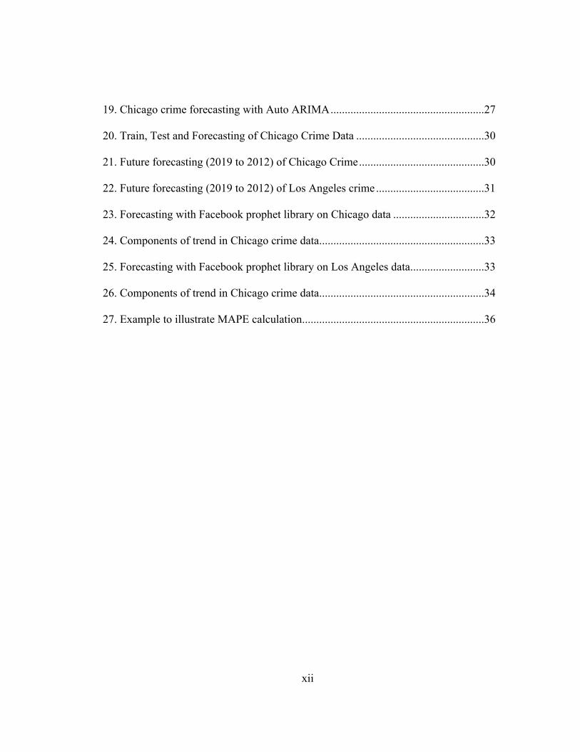
measures to prevent the occurrence of this type of crime. Figure 14 shows the top 10

dangerous areas in Chicago. According to the observation, crimes happening on streets,

residence and apartments is very high. These visualizations can help to create awareness

to the immigrants and visitors of these cities to take necessary steps against the occur-

rence of crime.

Figure 13: Top 10 Crime Types in Chicago

21

Figure 14: Top 10 Crime happening Locations in Chicago

This chapter summarizes the weekly, monthly and yearly trend of crimes with

visualizations. It is identified that Summers have high crime rate in Chicago and winters

have high crime rate in Los Angeles. Both cities have high crime rates on Friday eve-

nings. Identifying the trends and seasonality of the data, next chapter in this report de-

scribes different forecasting techniques to forecast crime for next one year.

22

Chapter 6

Time Series Forecasting of crime Data

Time Series is the succession of estimations of same variable gathered after some

time [13]. Time Series Analysis help in understanding the underlying trends, seasonality

and patterns in the data. As the variable is time dependent, trends and seasonality change

along with time. Forecasting of future events can be performed on such data which is de-

pendent on Time.

In this chapter, crime data is forecasted using previous events that are dependent

on time. To demonstrate this with an example, next month sales of a grocery store is an

unknown random variable. But this value can be relatively closer to last month sales data.

So, to forecast next month sales we consider past few months sales information. But to

forecast sales after a month in next year, we need to observe the trends and patterns in the

sales data for this year and last year. Here the assumption is January 2020 sales can be

like January 2019 and January 2018. But forecasting sales for next three years is even

more random as variables change along with time and last year data is less likely to be

useful. So, the further in future we try to forecast the more uncertain it is to predict [14].

This chapter discusses time series forecasting methods such as Auto Regressive

Integrated Moving Average (ARIMA), Auto ARIMA, Exponential Smoothing Model

23

(Holt’s Winter) and Facebook open source API prophet. This project compares the fore-

casting results of different methods and compares the forecasting results between Chica-

go and Los Angeles.

6.1 ARIMA:

ARIMA is a forecasting technique that estimates the future values of a time series

based completely on its own latency. [15]. ARIMA is general model which is accurate

enough to remove residual autocorrelation. The input time series to ARIMA model

should be a stationary time series and this stationarity is achieved by either differencing

or logging. A time series is said to be stationary if its mean (average), standard deviation,

variance, auto correlation etc. are standard with time [16].

The first step for implementing ARIMA is to make the series stationary. It is im-

portant to find that given series is stationary or non-stationary. As mentioned, stationary

series have constant mean, variance with time. They are just random series like white

noise. On the other hand, non-stationary series have trend and seasonality. Figure 15

shows Chicago Time series with weekly crime count.

24

Figure 15: Chicago Crime Time Series

Chicago data shows a decreasing downward trend and high seasonality during summers.

To analyze stationarity of data, Dicky Fuller stationary test is performed using python as

shown in figure 16.

Figure 16: Dicky Fullers stationarity test on Chicago time series data.

Differencing and de trending makes series stationary. After differencing the data,

Dicky Fullers test is again conducted to check stationary, constant mean and standard de-

25

viation on time series and results shows that the series are stationary now. Figure 17

shows the results of Dicky Fullers test after differencing. Differencing made the data sta-

tionary.

Figure 17: Dicky Fuller’s stationary test results on Chicago crime Data

The most important step in ARIMA is choosing the order of the ARIMA model.

In general, it is said that p, d, q values specifies the order of ARIMA [17]. ‘p’ indicates

AR (Auto Regressive) component, it describes number of previous values used to fore-

cast the future value. ‘d’ is the level of logging or differencing in the component. This

degree of differencing makes the series stationary. ‘q’ states the error in the model as ag-

gregation of past error values. Auto regressive, differencing and moving average make up

non-seasonal ARIMA model as a linear equation

X t = a + Ф1 xd t-1 + Фp xd t-p + ...+ θ1 e t-1+ θq e t-q +e t

26

Where X t represents the series in time, xd is X differenced d times, a is constant, Ф and θ

are model parameters [17].

In this project ARIMA model is implemented by using ARIMA package from

‘statsmodel’. p, d, q values are discovered with hyper parameter optimization. ARIMA

forecasting gives the lower and upper limit for the future crime and average crimes that

might occur in future. This forecasting a bit complicated for me to implement by deriving

the p, d, q values. Figure 18 shows ARIMA forecasting with Chicago data. The derived p,

d, q values are not good enough to make the model accurate for forecasting.

Figure 18: ARIMA forecasting with Chicago crime data

6.2 Auto ARIMA:

Auto ARIMA found to be a useful solution for this project. ARIMA requires lot

of processing such as making series stationary and determination of p, d, q vales. As this

27

project data set has 2 million records hyper parameter optimizations of ‘p, d, q values’ is

time consuming. Auto ARIMA eliminates the process of calculating p, d, q values. It can

directly fit the data into model and do forecasting. Python has libraries to import Auto

ARIMA. ‘pmdarima’ package from ‘Anaconda’ package installer is installed to imple-

ment this model. Weekly crime count is given as input to the model. Figure 19 shows the

test and forecasting results of the Chicago crime data.

figure 19: Chicago crime forecasting with Auto ARIMA

6.3 Holt’s Winter Forecasting:

This method is also known as ‘Triple Exponential Smoothing’. Simple Exponen-

tial Smoothing, double exponential smoothing can be used to forecast time series. Triple

Exponential Smoothing is more suitable for data with high seasonality and trend. Engi-

neering Statistics handbook says that past observations are weighted equally in single

moving averages. In contrast in exponential higher value weights are assigned to recent

values. This summarizes that older observations have relatively less weights than new

observations [18]. The equal of Single Exponential Smoothing is given as

28

St = αyt−1+ (1−α)St−1 0< α ≤ 1 t≥3.

Si stands for smoothing observation, y stands of original observation

Subscripts are time periods 1,2, 3...n.

α is the smoothing constant

This single Exponential Smoothing is for time series data with no trend and seasonality.

To deal with trends in the data, two constants are required in equation. The two equations

in double exponential smoothing are

St = αyt + (1−α)(St−1+bt−1) 0≤α≤1

Bt = γ(St−St−1) + ( 1−γ)bt−1 0≤γ≤1

α, γ are the smoothing constants. [18]

The first equation adjusts St directly for the trend of the previous period, bt−1, by

adding it to the previous smoothed value, St−1. This contributes to removal of lag and so

that St is now an appropriate current value. The second equation improves the trend,

which is showed as the difference between the last and its previous value. This equation

is different from basic single exponential smoothing as the trend is included here [18].

There are many cases where data shows trend and seasonality. In figure 15, Chi-

cago time series data observed as high downward trend and high seasonality. Every year

crime count is increasing in summer and decreasing in winter showing seasonality. For

data like this to forecast future crimes, both trend and seasonality need to be considered.

There comes the need of third level of Exponential Smoothing [18].

29

St= α yt/ It−L +(1−α) (St−1+bt−1) complete Smoothing

bt = γ(St−St−1) + (1−γ) bt−1 Trend Smoothing

It = β (yt / St) +(1−β) It−L Seasonal Smoothing

Ft+m = (St+mbt) + It-L+m Forecast

‘y’ is the observation, ‘S’ is the smoothed value, ‘b’ is the trend indicator

‘I’ is the represents seasonality, ‘F’ is m periods a head prediction, ‘t’ represents a time

interval. α, β, and γ are time intervals. [18]

In this project, Holt’s Winter (Triple exponential Smoothing) is considered for

crime forecasting. Project implements Holt’s Winter in python. From python library

‘statsmodels’ Hots and Exponential Smoothing packages need to be imported. Data is

divided into train and test samples in such a way that 2011 to early 2016 is considered for

training and mid 2016 to 2018 October is considered for testing. Holt’s winter model is

applied on training data and plotted with ‘matplotlib’ library for forecasting.

30

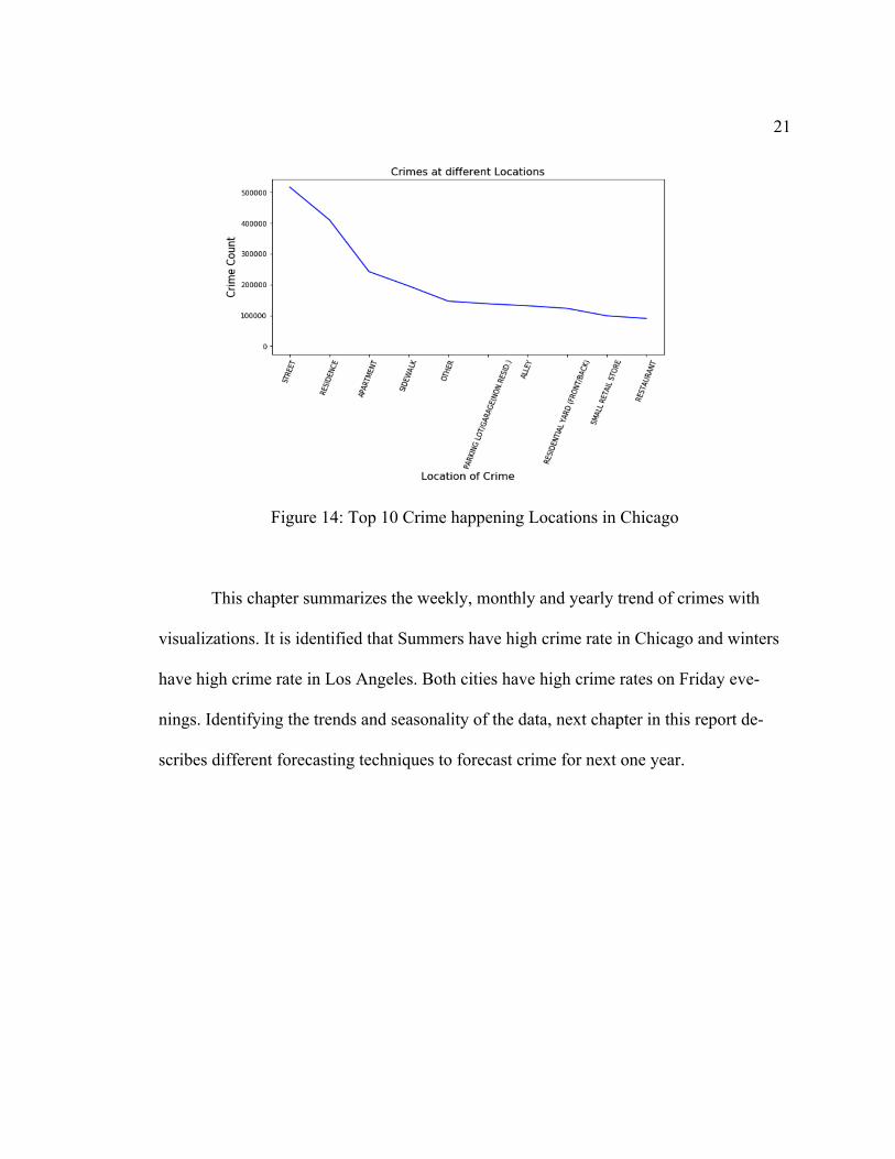
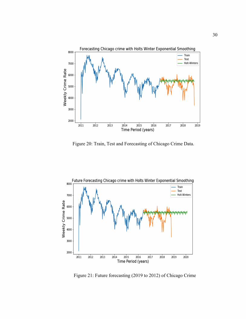
Figure 20: Train, Test and Forecasting of Chicago Crime Data.

Figure 21: Future forecasting (2019 to 2012) of Chicago Crime

31

Figure 22: Future forecasting (2019 to 2012) of Los Angeles crime

Holt’s Winter model is applied on Los Angeles Crime data to forecast the future

crime. Figure 20 shows the train, test and forecasting of Chicago crime per week with

available data. Figure 21 shows the future crime forecasting on Chicago crime data for

2019 to 2020. Figure 9 and 10 represents the same with Los Angeles crime data. Fore-

casting shows that there are around 5500 crimes per week in Chicago for next one year.

6.4 Facebook Prophet:

Prophet is forecasting model for time series data which can handle yearly, weekly,

and daily seasonality including holiday effects. When the data is time dependent and has

high history for seasonality prophet is the best model to forecast [10]. According to

Prophet documentation in GitHub, Facebook uses prophet for many reliable forecasts and

32

robust to outliers and missing data. Prophet API is available both is R and Python for

forecasting. It is an open source library and can be installed used Anaconda.

In this project, monthly weekly and daily data forecasting is performed on Chica-

go and Los Angeles crime Data. Forecasting for future time is mentioned in the model.

Facebook prophet also gives, yearly weekly and monthly trend of crimes. These insights

from visualizations gives the understanding of underlying patterns in the data.

Figure 23: Forecasting with Facebook prophet library on Chicago data

33

Figure 24: Components of trend in Chicago crime data

Figure 25: Forecasting with Facebook prophet library on Los Angeles data

34

Figure 26: Components of trend in Chicago crime data

In this report, chapter 7 mentions the model correctness and error measurement

techniques for the forecasting models. Results of the project work are discussed with pre-

vious work results mentioned in chapter 2.

35

Chapter 7

Error Measurement

This project forecasts the crime rate with different methods such as Auto ARIMA,

Holt’s Winter and Facebook prophet. The crucial step here is to verify the model correct-

ness by doing error measurement. It is important to know the deviation of forecasting to

the actual data. For this process, initially data is divided in training and testing and the

error analysis is performed on testing data. Later, the model is applied to future dates to

predict the crime rate. This chapter describes the error measurement technique used for

this project.

One of the better ways to measure error for forecasting techniques is Mean Abso-

lute Percentage Error (MAPE). [19] Good forecasting models have low values of MAPE.

In forecasting, forecasting value can be less than or greater than the actual value. For ex-

ample, in this project if the number of actual crimes are 570 per week, forecasting value

can be either 540 or 600. In both the cases the absolute error |570-600| or |570-540| is 30.

Mean of all such absolute errors is calculated and percentage is taken of such Mean Ab-

solute Errors in MAPE. Figure 27 gives an example to understand MAPE.

36

Figure 27 Example to illustrate MAPE calculation [20]

MAPE for the models is calculated using python ‘sklearn mean absolute error’ li-

brary. Error comparisons of forecasting models with MAPE is shown in Table 1. MAPE

for one year ahead forecasting on Chicago data with Auto ARIMA is 31 and with Los

Angeles is 6.5. MAPE with Holt’s winter for one year forecasting is 8.9 with Chicago

data and 5.5 with Los Angeles data. Facebook prophet has given better results compared

to Holt’s winter and ARIMA with MAPE of 4 and 4.02 with Chicago and Los Angeles

data. Even though in this project, Facebook prophet worked well, in practical cases it is a

bit difficult to do parameter tuning with it.

Table 1: Error comparisons of forecasting models

Model MAPE with Chicago

weekly data

MAPE with Los An-

geles weekly data

Auto ARIMA 31 6.5

Holt’s Winter 8.9 5.5

Facebook Prophet 4.2 4.02

37

‘Forecasting Crimes Using Autoregressive Models’, mentioned in Literature Re-

view chapter states ARIMA is the best model to forecast Chicago crime data in 2015 with

MAPE of 16 over 6 months forecasting. In this project, Holt’s winter and Facebook

prophet libraries are better with one year forecasting on Chicago data with MAPE 8 and

4. This shows an improvement in forecasting compared to the ARIMA model mentioned

in ‘Forecasting Crimes Using Autoregressive Models’.

38

Chapter 8

Conclusion

Time Series Analysis and Forecasting is performed with several visualizations

and statistical models in this project. Holt’s winter and Facebook prophet forecasting

models gave good forecasting for next one year with less MAPE. According to forecast-

ing results for the year 2019 Chicago crimes are slightly decreasing with high around

5000 crimes per week in summer and low around 1000 crimes per week in winter. Re-

sults show that Los Angeles crime vary around 4000 per week. This forecasting results

can help police to take necessary precautions according to the crime rate.

Crime Data analyzing with visualizations states that Summers are dangerous in

Chicago and Friday evenings from 4 pm to 8 pm have high crime occurrences. This helps

tourists, students and immigrants to plan safer travels and stay safe during their stay. Los

Angeles have slightly high crimes during winter and Friday evenings compared to other

seasons and days. The overall trend with crime data is decreasing in both the cities from

2011 to 2018. There are more thefts in Chicago on streets from past 8 years. Government

of USA can utilize these results to increase more police force during hotter months and

weekends in Chicago.

With this project work, I want to let the reader know that data analysis, visualiza-

tion and forecasting could be used for a large variety of data sets, which could reveal

39

things that haven’t been observed before. This could help the targeted audience in under-

standing of how things are going to be for the foreseeable future with some confidence

backed by the algorithms developed by geniuses. In my experience analyzing crime data,

I developed a positive hope for safer future after observing a downward trend in the

crime rate. This project excited me about the possible constructive impact it might create

in future. Future work with this analysis is to predict the location of crime and tag the

crime activities to a geographical map.

40

REFERENCES

[1] Crime Rates. [Online]. Available: https://www.neighborhoodscout.com/il/chicago/crime [Accessed 2-March-2019].

[2] Chicago and Los Angeles Crime Datasets. [Online]. Available:

https://catalog.data.gov/dataset [Accessed 2-March-2019]. [3] E. Cesario, C. Catlett and D. Talia, “Forecasting Crimes Using Autoregressive Mod-

els,” IEEE 14th Intl Conf on Dependable, Autonomic and Secure Computing, 14th Intl Conf on Pervasive Intelligence and Computing, 2nd Intl Conf on Big Data In-telligence and Computing and Cyber Science and Technology Con-gress(DASC/PiCom/DataCom/CyberSciTech), pp. 795-802, Auckland, 2016.

[4] G. Wilpen, O.Andreas and T.Yvonne, “Short-term forecasting of crime,” Internation-

al Journal of Forecasting, Volume 19, Issue 4, pp. 579-594, October–December 2003.

[4] L. McClendon and N. Meghanathan, “Using Machine Learning Algorithms to Ana-

lyze Crime Data,” Machine Learning and Applications: An International Journal (MLAIJ), Vol.2, No.1, March 2015. [Online]. Available: http://airccse.org/journal/mlaij/papers/2115mlaij01.pdf [Accessed 10-March-2019].

[6] Proven Crime Reduction Results. [online]. Available:

http://www.predpol.com/results/ [Accessed 6-March-2019]. [7] U. Thongsatapornwatana, “A survey of data mining techniques for analyzing crime

patterns,” the 2nd Asian Conference on Defence Technology (ACDT), Chiang Mai, 2016. pp. 123-128.

[8] B. Chandra, M. Gupta and M. P. Gupta, “A multivariate time series clustering ap-

proach for crime trends prediction,” IEEE International Conference on Systems, Man and Cybernetics, Singapore, 2008. pp. 892-896.

[9] S. Seabold and J. Perktold, “Statsmodels: Econometric and statistical modeling with

python,” proceedings of the 9th Python in Science Conference, 2010. [10] Forecasting at Scale. [Online]. Available: https://facebook.github.io/prophet/ [Ac-

cessed 6-April-2019]. [11] Chicago Crimes from 2001 to present [Online]. Available:

https://data.cityofchicago.org/Public-Safety/Crimes-2001-to-present/ijzp-q8t2 [Accessed 6-April-2019].

41

[12] Los Angeles Crimes from 2010 to present [Online]. Available:

https://catalog.data.gov/dataset/crime-data-from-2010-to-present [Accessed 6-April-2019].

[13] Overview of Time Series Characteristics. [Online]. Available:

https://newonlinecourses.science.psu.edu/stat510/node/47/ [Accessed 1-April-2019].

[14] H. Robin John and A. George, Forecasting Principles and Practice, 2nd ed, May

2018. [E-book]. Available: https://otexts.com/fpp2/ [Accessed 1-April-2019]. [15] Auto Regressive Integrated Moving Average Models. [Online]. Available:

http://www.forecastingsolutions.com/arima.html [Accessed 7- April-2019]. [16] Madhav Mishra, “Unboxing ARIMA models”. [Online]. Available:

https://towardsdatascience.com/unboxing-arima-models-1dc09d2746f8 [Accessed 5-April-2019].

[17] Ruslana Dalinina, “Introduction to Forecasting with ARIMA in R”. [Online]. Avila-

ble: https://www.datascience.com/blog/introduction-to-forecasting-with-arima-in-r-learn-data-science-tutorials [Accessed 8-April-2019].

[18] NIST/SEMATECH e-Handbook of Statistical Methods, April 2012. [E-book]. Avail-

able: https://www.itl.nist.gov/div898/handbook [Accessed 30-March-2019]. [19] H. Chen and L. Wu, “A new measure of forecast accuracy,” the 2nd IEEE Interna-

tional Conference on Information and Financial Engineering, Chongqing, 2010. pp. 710-712.

[20] A Guide to Forecast Error Measurement Statistics and How to Use Them. [Online].

Available: http://www.forecastpro.com/Trends/forecasting101August2011.html [Accessed 5- April-2019].