Time Response Chapter Learning Outcomes After completing this chapter the student will be able to: • Use poles and zeros of transfer functions to determine the time response of a control system (Sections 4.1–4.2) • Describe quantitatively the transient response of first-order systems (Section 4.3) • Write the general response of second-order systems given the pole location (Section 4.4) • Find the damping ratio and natural frequency of a second-order system (Section 4.5) • Find the settling time, peak time, percent overshoot, and rise time for an underdamped second-order system (Section 4.6) • Approximate higher-order systems and systems with zeros as first- or second- order systems (Sections 4.7–4.8) • Describe the effects of nonlinearities on the system time response (Section 4.9) • Find the time response from the state-space representation (Sections 4.10–4.11) Case Study Learning Outcomes You will be able to demonstrate your knowledge of the chapter objectives with case studies as follows: • Given the antenna azimuth position control system shown on the front endpapers, you will be able to (1) predict, by inspection, the form of the open-loop angular velocity response of the load to a step voltage input to 4 157

Welcome message from author
This document is posted to help you gain knowledge. Please leave a comment to let me know what you think about it! Share it to your friends and learn new things together.
Transcript

Time Response
Chapter Learning Outcomes
After completing this chapter the student will be able to:
• Use poles and zeros of transfer functions to determine the time response of a
control system (Sections 4.1–4.2)
• Describe quantitatively the transient response of first-order systems (Section 4.3)
• Write the general response of second-order systems given the pole location
(Section 4.4)
• Find the damping ratio and natural frequency of a second-order system (Section 4.5)
• Find the settling time, peak time, percent overshoot, and rise time for an
underdamped second-order system (Section 4.6)
• Approximate higher-order systems and systems with zeros as first- or second-
order systems (Sections 4.7–4.8)
• Describe the effects of nonlinearities on the system time response (Section 4.9)
• Find the time response from the state-space representation (Sections 4.10–4.11)
Case Study Learning Outcomes
You will be able to demonstrate your knowledge of the chapter objectives with case
studies as follows:
• Given the antenna azimuth position control system shown on the front
endpapers, you will be able to (1) predict, by inspection, the form of the
open-loop angular velocity response of the load to a step voltage input to
�4157

the power amplifier; (2) describe quantitatively the transient responseof the open-loop system; (3) derive the expression for the open-loop
angular velocity output for a step voltage input; (4) obtain the open-loop
state-space representation; (5) plot the open-loop velocity step response
using a computer simulation.
• Given the block diagram for the Unmanned Free-Swimming Submersible (UFSS)vehicle’s pitch control system shown on the back endpapers, you will be able to
predict, find, and plot the response of the vehicle dynamics to a step input
command. Further, you will be able to evaluate the effect of system zeros and
higher-order poles on the response. You also will be able to evaluate the roll
response of a ship at sea.
4.1 Introduction
In Chapter 2, we saw how transfer functions can represent linear, time-invariant systems.
In Chapter 3, systems were represented directly in the time domain via the state and output
equations. After the engineer obtains a mathematical representation of a subsystem,
the subsystem is analyzed for its transient and steady-state responses to see if these
characteristics yield the desired behavior. This chapter is devoted to the analysis of system
transient response.
It may appear more logical to continue with Chapter 5, which covers the modeling
of closed-loop systems, rather than to break the modeling sequence with the analysis
presented here in Chapter 4. However, the student should not continue too far into system
representation without knowing the application for the effort expended. Thus, this chapter
demonstrates applications of the system representation by evaluating the transient
response from the system model. Logically, this approach is not far from reality, since
the engineer may indeed want to evaluate the response of a subsystem prior to inserting it
into the closed-loop system.
After describing a valuable analysis and design tool, poles and zeros, we begin
analyzing our models to find the step response of first- and second-order systems. The order
refers to the order of the equivalent differential equation representing the system—the
order of the denominator of the transfer function after cancellation of common factors
in the numerator or the number of simultaneous first-order equations required for the
state-space representation.
4.2 Poles, Zeros, and System Response
The output response of a system is the sum of two responses: the forced response and the
natural response.1 Although many techniques, such as solving a differential equation or
taking the inverse Laplace transform, enable us to evaluate this output response, these
techniques are laborious and time-consuming. Productivity is aided by analysis and design
techniques that yield results in a minimum of time. If the technique is so rapid that we feel
we derive the desired result by inspection, we sometimes use the attribute qualitative to
describe the method. The use of poles and zeros and their relationship to the time response of
a system is such a technique. Learning this relationship gives us a qualitative “handle” on
problems. The concept of poles and zeros, fundamental to the analysis and design of control
1The forced response is also called the steady-state response or particular solution. The natural response is also
called the homogeneous solution.
158 Chapter 4 Time Response

systems, simplifies the evaluation of a system’s response. The reader is encouraged to
master the concepts of poles and zeros and their application to problems throughout this
book. Let us begin with two definitions.
Poles of a Transfer FunctionThe poles of a transfer function are (1) the values of the Laplace transform variable, s, that
cause the transfer function to become infinite or (2) any roots of the denominator of the
transfer function that are common to roots of the numerator.
Strictly speaking, the poles of a transfer function satisfy part (1) of the definition.
For example, the roots of the characteristic polynomial in the denominator are values of
s that make the transfer function infinite, so they are thus poles. However, if a factor of
the denominator can be canceled by the same factor in the numerator, the root of this
factor no longer causes the transfer function to become infinite. In control systems, we
often refer to the root of the canceled factor in the denominator as a pole even though
the transfer function will not be infinite at this value. Hence, we include part (2) of the
definition.
Zeros of a Transfer FunctionThe zeros of a transfer function are (1) the values of the Laplace transform variable, s, that
cause the transfer function to become zero, or (2) any roots of the numerator of the transfer
function that are common to roots of the denominator.
Strictly speaking, the zeros of a transfer function satisfy part (1) of this definition. For
example, the roots of the numerator are values of s that make the transfer function zero and
are thus zeros. However, if a factor of the numerator can be canceled by the same factor in
the denominator, the root of this factor no longer causes the transfer function to become
zero. In control systems, we often refer to the root of the canceled factor in the numerator as
a zero even though the transfer function will not be zero at this value. Hence, we include part
(2) of the definition.
Poles and Zeros of a First-Order System: An ExampleGiven the transfer function G(s) in Figure 4.1(a), a pole exists at s � �5, and a zero exists at�2. These values are plotted on the complex s-plane in Figure 4.1(b), using an× for the pole
and a ○ for the zero. To show the properties of the poles and zeros, let us find the unit
step response of the system. Multiplying the transfer function of Figure 4.1(a) by a step
function yields
C�s� � �s � 2�s�s � 5� � A
s� B
s � 5� 2=5
s� 3=5
s � 5�4.1�
where
A � �s � 2��s � 5�
s®0
� 2
5
B � �s � 2�s
s®�5� 3
5
Thus,
c�t� � 2
5� 3
5e�5t �4.2�
4.2 Poles, Zeros, and System Response 159

From the development summarized in Figure 4.1(c), we draw the following
conclusions:
1. A pole of the input function generates the form of the forced response (that is, the pole at
the origin generated a step function at the output).
2. A pole of the transfer function generates the form of the natural response (that is, the pole
at �5 generated e�5t).
3. A pole on the real axis generates an exponential response of the form e�αt, where �α is
the pole location on the real axis. Thus, the farther to the left a pole is on the negative real
axis, the faster the exponential transient response will decay to zero (again, the pole at�5generated e�5t; see Figure 4.2 for the general case).
G(s)
C(s)1s
(b)(a)
jω
s-plane
1s
s + 2
jω jω jω
Input pole System zero System pole
Outputtransform
2/5+
3/5
s + 5
2
5
3
5e–5t
Outputtime
response+
Forced response Natural response
(c)
–5
R(s) = s + 2
1
s + 5
C(s) =
c(t) =
s
–2 –5
s-planes-planes-plane
s + 5–2
σ
σ
σσ
FIGURE 4.1 a. System showing input and output; b. pole-zero plot of the system; c. evolution of a
system response. Follow blue arrows to see the evolution of the response component generated by the
pole or zero.
Pole at – α generatesresponse Ke– αt
s-plane
jω
– α
σ
FIGURE 4.2 Effect of a real-axis pole upon transient response.
160 Chapter 4 Time Response

4. The zeros and poles generate the amplitudes for both the forced and natural responses
(this can be seen from the calculation of A and B in Eq. (4.1)).
Let us now look at an example that demonstrates the technique of using poles to obtain
the form of the system response. We will learn to write the form of the response by
inspection. Each pole of the system transfer function that is on the real axis generates an
exponential response that is a component of the natural response. The input pole generates
the forced response.
Example 4.1
Evaluating Response Using PolesEvaluating Response Using Poles
PROBLEM: Given the system of Figure 4.3, write the output, c(t), in
general terms. Specify the forced and natural parts of the solution.
SOLUTION: By inspection, each system pole generates an exponential
as part of the natural response. The input’s pole generates the forced
response. Thus,
C s� � � K1
s
Forcedresponse
� K2
s � 2� K3
s � 4� K4
s � 5
Naturalresponse
�4.3�
Taking the inverse Laplace transform, we get
c�t� � K1
Forcedresponse
�K2e�2t � K3e
�4t � K4e�5t
Naturalresponse
�4.4�
(s + 2)(s + 4)(s + 5)
C(s)1sR(s) = (s + 3)
FIGURE 4.3 System for Example 4.1
Skill-Assessment Exercise 4.1
PROBLEM: A system has a transfer function, G�s� � 10�s � 4��s � 6��s � 1��s � 7��s � 8��s � 10�.
Write, by inspection, the output, c(t), in general terms if the input is a unit step.
ANSWER: c�t� � A � Be�t � Ce�7t � De�8t � Ee�10t
In this section, we learned that poles determine the nature of the time response:
Poles of the input function determine the form of the forced response, and poles
of the transfer function determine the form of the natural response. Zeros and poles
of the input or transfer function contribute to the amplitudes of the component
parts of the total response. Finally, poles on the real axis generate exponential
responses.
4.2 Poles, Zeros, and System Response 161

4.3 First-Order Systems
We now discuss first-order systems without zeros to define a performance
specification for such a system. A first-order system without zeros can be
described by the transfer function shown in Figure 4.4(a). If the input is a
unit step, where R�s� � 1=s, the Laplace transform of the step response is
C(s), where
C�s� � R�s�G�s� � a
s�s � a� �4.5�
Taking the inverse transform, the step response is given by
c�t� � cf �t� � cn�t� � 1 � e�at �4.6�
where the input pole at the origin generated the forced response cf �t� � 1, and the system
pole at �a, as shown in Figure 4.4(b), generated the natural response cn�t� � �e�at .Equation (4.6) is plotted in Figure 4.5.
Let us examine the significance of parameter a, the only parameter needed to describe
the transient response. When t � 1=a,
e�at j t�1=a � e�1 � 0:37 �4.7�or
c�t�j t�1=a � 1 � e�at j t�1=a � 1 � 0:37 � 0:63 �4.8�
We now use Eqs. (4.6), (4.7), and (4.8) to define three transient response performance
specifications.
Time ConstantWe call 1/a the time constant of the response. From Eq. (4.7), the time constant can be
described as the time for e�at to decay to 37% of its initial value. Alternately, from Eq. (4.8)
the time constant is the time it takes for the step response to rise to 63% of its final value
(see Figure 4.5).
aR(s)
(a)
jω
–a
(b)
s + a
G(s)
C(s)
s-plane
σ
FIGURE 4.4 a. First-order system; b. pole plot
Virtual Experiment 4.1
First-Order
Transfer Function
Put theory into practice and find
a first-order transfer function
representing the Quanser
Rotary Servo. Then validate the
model by simulating it in
LabVIEW. Such a servo motor
is used in mechatronic gadgets
such as cameras.
Virtual experiments are found
on Learning Space.
t
1.0
0.9
0.8
0.7
0.6
0.5
0.4
0.3
0.2
0.1
0
Ts
Tr
a1
a2
a3
a4
a5
Initial slope =
c(t)1
time constant
63% of Hnal valueat t = one time constant
= a
FIGURE 4.5 First-order system response to a unit step
162 Chapter 4 Time Response

The reciprocal of the time constant has the units (1/seconds), or frequency. Thus, we
can call the parameter a the exponential frequency. Since the derivative of e�at is �a when
t � 0, a is the initial rate of change of the exponential at t � 0. Thus, the time constant can be
considered a transient response specification for a first-order system, since it is related to the
speed at which the system responds to a step input.
The time constant can also be evaluated from the pole plot (see Figure 4.4(b)). Since
the pole of the transfer function is at �a, we can say the pole is located at the reciprocal of
the time constant, and the farther the pole from the imaginary axis, the faster the transient
response.
Let us look at other transient response specifications, such as rise time, T r, and settling
time, T s, as shown in Figure 4.5.
Rise Time,TrRise time is defined as the time for the waveform to go from 0.1 to 0.9 of its final value. Rise
time is found by solving Eq. (4.6) for the difference in time at c�t� � 0:9 and c�t� � 0:1.Hence,
Tr � 2:31
a� 0:11
a� 2:2
a�4.9�
Settling Time,TsSettling time is defined as the time for the response to reach, and stay within, 2% of its
final value.2 Letting c�t� � 0:98 in Eq. (4.6) and solving for time, t, we find the settling
time to be
T s � 4
a�4.10�
First-Order Transfer Functions via TestingOften it is not possible or practical to obtain a system’s transfer function analytically.
Perhaps the system is closed, and the component parts are not easily identifiable. Since the
transfer function is a representation of the system from input to output, the system’s step
response can lead to a representation even though the inner construction is not known. With
a step input, we can measure the time constant and the steady-state value, from which the
transfer function can be calculated.
Consider a simple first-order system, G�s� � K=�s � a�, whose step response is
C�s� � K
s�s � a� � K=a
s� K=a
�s � a� �4.11�
If we can identify K and a from laboratory testing, we can obtain the transfer function of the
system.
For example, assume the unit step response given in Figure 4.6. We determine that it
has the first-order characteristics we have seen thus far, such as no overshoot and nonzero
initial slope. From the response, we measure the time constant, that is, the time for the
amplitude to reach 63% of its final value. Since the final value is about 0.72, the time
constant is evaluated where the curve reaches 0:63 � 0:72 � 0:45, or about 0.13 second.
Hence, a � 1=0:13 � 7:7.
2 Strictly speaking, this is the definition of the 2% setting time. Other percentages, for example 5%, also can be used.
We will use settling time throughout the book to mean 2% settling time.
4.3 First-Order Systems 163

To find K, we realize from Eq. (4.11) that the forced response reaches a steady-state
value of K=a � 0:72. Substituting the value of a, we find K � 5:54. Thus, the transfer
function for the system is G�s� � 5:54=�s � 7:7�. It is interesting to note that the response ofFigure 4.6 was generated using the transfer function G�s� � 5=�s � 7�.
4.4 Second-Order Systems: Introduction
Let us now extend the concepts of poles and zeros and transient response to second-order
systems. Compared to the simplicity of a first-order system, a second-order system exhibits
a wide range of responses that must be analyzed and described. Whereas varying a
first-order system’s parameter simply changes the speed of the response, changes in the
parameters of a second-order system can change the form of the response. For example, a
second-order system can display characteristics much like a first-order system, or, depending
on component values, display damped or pure oscillations for its transient response.
To become familiar with the wide range of responses before formalizing our
discussion in the next section, we take a look at numerical examples of the second-order
system responses shown in Figure 4.7. All examples are derived from Figure 4.7(a), the
general case, which has two finite poles and no zeros. The term in the numerator is simply a
scale or input multiplying factor that can take on any value without affecting the form of the
derived results. By assigning appropriate values to parameters a and b, we can show all
possible second-order transient responses. The unit step response then can be found using
0 0.1 0.2 0.3 0.4 0.5 0.6 0.7 0.8
0.1
0.2
0.3
0.4
0.5
0.6
0.7
0.8
Time (seconds)
Am
pli
tude
FIGURE 4.6 Laboratory results of a system step response test
Skill-Assessment Exercise 4.2
PROBLEM: A system has a transfer function, G�s� � 50
s � 50. Find the time constant, Tc,
settling time, Ts, and rise time, T r.
ANSWER: Tc � 0:02 s; T s � 0:08 s; and T r � 0:044 s:
The complete solution is located at www.wiley.com/college/nise.
164 Chapter 4 Time Response

C�s� � R�s�G�s�, where R�s� � 1=s, followed by a partial-fraction expansion and the inverseLaplace transform. Details are left as an end-of-chapter problem, for which you may want to
review Section 2.2.
We now explain each response and show how we can use the poles to determine the
nature of the response without going through the procedure of a partial-fraction expansion
followed by the inverse Laplace transform.
Overdamped Response, Figure 4.7(b)For this response,
C�s� � 9
s�s2 � 9s � 9� � 9
s�s � 7:854��s � 1:146� �4.12�
This function has a pole at the origin that comes from the unit step input and two real poles
that come from the system. The input pole at the origin generates the constant forced
response; each of the two system poles on the real axis generates an exponential natural
response whose exponential frequency is equal to the pole location. Hence, the output
initially could have been written as c�t� � K1 � K2e�7:854t � K3e
�1:146t. This response,
b
s2 + as + b
1 2 3 4 5t
0.5
1.0
c(t) c(t) = 1 + 0.171e–7.854t –
9
G(s)
C(s)
General
System
(a)
(b)
(c)
(d)
(e)
Overdamped
Pole-zero plot
G(s)
–7.854 –1.146
0
0.8
1.2
c(t) = 1–e–t(cos 8t + sin 8t)
9
G(s)
C(s)
Underdamped
s-plane
–1 0.4
=1–1.06e–t cos( 8t–19.47°)
1 2 3 4 5t
0
1
2
c(t)
c(t) = 1 – cos 3t
9
G(s)
C(s)
Undamped
j3
1 2 3 4 5t
0
1.0
c(t)
c(t) = 1 – 3te–3t – e–3t
9
G(s)
C(s)
Critically damped
–3
0.80.60.40.2
Response
jω
jω
jω
s-plane
s-plane
s-plane
s2 + 9s + 9
s2 + 2s + 9
s2 + 9
s2 + 6s + 9
jω
–j3
c(t)
C(s)
88
0.2
1.0
1.4
0.6
R(s) =1s
R(s) =1s
R(s) =1s
R(s) =1s
R(s) =1s
8
8
1 2 3 4 5t
j
j
0
1.171e–1.146t
–
σ
σ
σ
σ
FIGURE 4.7 Second-order
systems, pole plots, and step
responses
4.4 Second-Order Systems: Introduction 165

shown in Figure 4.7(b), is called overdamped.3 We see that the poles tell us the form of the
response without the tedious calculation of the inverse Laplace transform.
Underdamped Response, Figure 4.7 (c)For this response,
C�s� � 9
s�s2 � 2s � 9� �4.13�
This function has a pole at the origin that comes from the unit step input and two complex poles
that come from the system. We now compare the response of the second-order system to the
poles that generated it. First wewill compare the pole location to the time function, and thenwe
will compare the pole location to the plot. FromFigure 4.7(c), the poles that generate the natural
response are at s � �1� jffiffiffi
8p
. Comparing these values to c(t) in the samefigure,we see that the
real part of the polematches the exponential decay frequencyof the sinusoid’s amplitude,while
the imaginary part of the pole matches the frequency of the sinusoidal oscillation.
Let us now compare the pole location to the plot. Figure 4.8
shows a general, damped sinusoidal response for a second-order
system. The transient response consists of an exponentially decaying
amplitudegeneratedbytherealpartof thesystempole timesasinusoidal
waveformgenerated by the imaginary part of the systempole. The time
constant of the exponential decay is equal to the reciprocal of the real
part of the system pole. The value of the imaginary part is the actual
frequency of the sinusoid, as depicted in Figure 4.8. This sinusoidal
frequency is given the name damped frequency of oscillation, ωd.
Finally, the steady-state response (unit step) was generated by the
input pole located at the origin. We call the type of response shown in
Figure 4.8 an underdamped response, one which approaches a steady-
state value via a transient response that is a damped oscillation.
The following example demonstrates how a knowledge of the
relationship between the pole location and the transient response
can lead rapidly to the response form without calculating the inverse
Laplace transform.
c(t)
Exponential decay generated by real part of complex pole pair
Sinusoidal oscillation generated byimaginary part of complex pole pair
t
FIGURE 4.8 Second-order step response components
generated by complex poles
Example 4.2
Form of Underdamped Response Using PolesForm of Underdamped Response Using Poles
PROBLEM: By inspection, write the form of the step response of the system in Figure 4.9.
SOLUTION: First we determine that the form of the forced response is a step.
Next we find the form of the natural response. Factoring the denominator of the
transfer function in Figure 4.9, we find the poles to be s � �5� j13:23. The realpart, �5, is the exponential frequency for the damping. It is also the reciprocal
of the time constant of the decay of the oscillations. The imaginary part, 13.23,
is the radian frequency for the sinusoidal oscillations. Using our previous discussion
and Figure 4.7(c) as a guide, we obtain c�t� � K1 � e�5t �K2 cos 13:23t �K3 sin 13:23t� �K1 � K4e
�5t�cos 13:23t � ϕ�, where ϕ � tan�1K3=K2; K4 �ffiffiffiffiffiffiffiffiffiffiffiffiffiffiffiffiffi
K22 � K2
3
p, and c(t) is a
constant plus an exponentially damped sinusoid.
200C(s)
s2 + 10s + 200
1s
R(s) =
FIGURE 4.9 System for
Example 4.2
3 So named because overdamped refers to a large amount of energy absorption in the system, which inhibits the
transient response from overshooting and oscillating about the steady-state value for a step input. As the energy
absorption is reduced, an overdamped system will become underdamped and exhibit overshoot.
166 Chapter 4 Time Response

We will revisit the second-order underdamped response in Sections 4.5 and 4.6,
where we generalize the discussion and derive some results that relate the pole position to
other parameters of the response.
Undamped Response, Figure 4.7(d)For this response,
C�s� � 9
s�s2 � 9� �4.14�
This function has a pole at the origin that comes from the unit step input and two imaginary
poles that come from the system. The input pole at the origin generates the constant forced
response, and the two system poles on the imaginary axis at � j3 generate a sinusoidal
natural response whose frequency is equal to the location of the imaginary poles. Hence, the
output can be estimated as c�t� � K1 � K4 cos�3t � ϕ�. This type of response, shown in
Figure 4.7(d), is called undamped. Note that the absence of a real part in the pole pair
corresponds to an exponential that does not decay. Mathematically, the exponential is
e�0t � 1.
Critically Damped Response, Figure 4.7 (e)For this response,
C�s� � 9
s�s2 � 6s � 9� � 9
s�s � 3�2 �4.15�
This function has a pole at the origin that comes from the unit step input and two multiple
real poles that come from the system. The input pole at the origin generates the constant
forced response, and the two poles on the real axis at �3 generate a natural response
consisting of an exponential and an exponential multiplied by time, where the exponential
frequency is equal to the location of the real poles. Hence, the output can be estimated as
c�t� � K1 � K2e�3t � K3te
�3t. This type of response, shown in Figure 4.7(e), is called
critically damped. Critically damped responses are the fastest possible without the over-
shoot that is characteristic of the underdamped response.
We now summarize our observations. In this section we defined the following natural
responses and found their characteristics:
1. Overdamped responses
Poles: Two real at �σ1; �σ2Natural response: Two exponentials with time constants equal to the reciprocal of the
pole locations, or
c�t� � K1e�σ1t � K2e
�σ2t
2. Underdamped responses
Poles: Two complex at �σd � jωd
Natural response: Damped sinusoid with an exponential envelope whose time
constant is equal to the reciprocal of the pole’s real part. The radian frequency of
the sinusoid, the damped frequency of oscillation, is equal to the imaginary part of the
poles, or
c�t� � Ae�σd t cos�ωdt � ϕ�
4.4 Second-Order Systems: Introduction 167

3. Undamped responses
Poles: Two imaginary at � jω1
Natural response: Undamped sinusoid with radian frequency equal to the imaginary part
of the poles, or
c�t� � A cos�ω1t � ϕ�4. Critically damped responses
Poles: Two real at �σ1Natural response: One term is an exponential whose time constant is equal to the
reciprocal of the pole location. Another term is the product of time, t, and an exponential
with time constant equal to the reciprocal of the pole location, or
c�t� � K1e�σ1t � K2te
�σ1t
The step responses for the four cases of damping discussed in this section are
superimposed in Figure 4.10. Notice that the critically damped case is the division between
the overdamped cases and the underdamped cases and is the fastest response without
overshoot.
0.5 1 1.5 2 2.5 3 3.5 40
0.2
0.4
0.6
0.8
1.0
1.2
1.4
1.6
1.8
2.0
Under-damped
Criticallydamped
Overdamped
c(t)
t
Undamped
FIGURE 4.10 Step responses for second-order system damping cases
Skill-Assessment Exercise 4.3
PROBLEM: For each of the following transfer functions, write, by inspection, the
general form of the step response:
a. G�s� � 400
s2 � 12s � 400
b. G�s� � 900
s2 � 90s � 900
c. G�s� � 225
s2 � 30s � 225
d. G�s� � 625
s2 � 625
168 Chapter 4 Time Response

In the next section, we will formalize and generalize our discussion of second-
order responses and define two specifications used for the analysis and design of
second-order systems. In Section 4.6, we will focus on the underdamped case and
derive some specifications unique to this response that we will use later for analysis and
design.
4.5 The General Second-Order System
Now that we have become familiar with second-order systems and their responses, we
generalize the discussion and establish quantitative specifications defined in such a way that
the response of a second-order system can be described to a designer without the need for
sketching the response. In this section, we define two physically meaningful specifications
for second-order systems. These quantities can be used to describe the characteristics of the
second-order transient response just as time constants describe the first-order system
response. The two quantities are called natural frequency and damping ratio. Let us
formally define them.
Natural Frequency, ωn
The natural frequency of a second-order system is the frequency of oscillation of the system
without damping. For example, the frequency of oscillation of a series RLC circuit with the
resistance shorted would be the natural frequency.
Damping Ratio, ζBefore we state our next definition, some explanation is in order. We have already seen
that a second-order system’s underdamped step response is characterized by damped
oscillations. Our definition is derived from the need to quantitatively describe this
damped oscillation regardless of the time scale. Thus, a system whose transient
response goes through three cycles in a millisecond before reaching the steady state
would have the same measure as a system that went through three cycles in a
millennium before reaching the steady state. For example, the underdamped curve
in Figure 4.10 has an associated measure that defines its shape. This measure
remains the same even if we change the time base from seconds to microseconds or
to millennia.
A viable definition for this quantity is one that compares the exponential decay
frequency of the envelope to the natural frequency. This ratio is constant regardless of the
time scale of the response. Also, the reciprocal, which is proportional to the ratio of
the natural period to the exponential time constant, remains the same regardless of the
time base.
ANSWERS:
a. c�t� � A � Be�6t cos�19:08t � ϕ�b. c�t� � A � Be�78:54t � Ce�11:46t
c. c�t� � A � Be�15t � Cte�15t
d. c�t� � A � B cos�25t � ϕ�
The complete solution is located at www.wiley.com/college/nise.
4.5 The General Second-Order System 169

We define the damping ratio, ζ, to be
ζ � Exponential decay frequency
Natural frequency �rad=second� � 1
2π
Natural period �seconds�Exponential time constant
Let us now revise our description of the second-order system to reflect the new
definitions. The general second-order system shown in Figure 4.7(a) can be transformed to
show the quantities ζ and ωn. Consider the general system
G�s� � b
s2 � as � b�4.16�
Without damping, the poles would be on the jω-axis, and the response would be an
undamped sinusoid. For the poles to be purely imaginary, a � 0. Hence,
G�s� � b
s2 � b�4.17�
By definition, the natural frequency, ωn, is the frequency of oscillation of this system. Since
the poles of this system are on the jω-axis at � jffiffiffi
bp
,
ωn �ffiffiffi
bp
�4.18�
Hence,
b � ω2n �4.19�
Now what is the term a in Eq. (4.16)? Assuming an underdamped system, the
complex poles have a real part, σ, equal to �a=2. The magnitude of this value is then the
exponential decay frequency described in Section 4.4. Hence,
ζ � Exponential decay frequency
Natural frequency �rad=second� � jσ jωn
� a=2
ωn
�4.20�
from which
a � 2ζωn �4.21�
Our general second-order transfer function finally looks like this:
G�s� � ω2n
s2 � 2ζωns � ω2n
�4.22�
In the following example we find numerical values for ζ and ωn by matching the
transfer function to Eq. (4.22).
170 Chapter 4 Time Response
Now that we have defined ζ and ωn, let us relate these quantities to the pole location.
Solving for the poles of the transfer function in Eq. (4.22) yields
s1; 2 � �ζωn �ωn
ffiffiffiffiffiffiffiffiffiffiffiffi
ζ2 � 1
q
�4.24�
From Eq. (4.24) we see that the various cases of second-order response are a function of ζ;
they are summarized in Figure 4.11.4
Example 4.3
Finding ζ and ωn For a Second-Order SystemFinding ζ and ωn For a Second-Order System
PROBLEM: Given the transfer function of Eq. (4.23), find ζ and ωn.
G�s� � 36
s2 � 4:2s � 36�4.23�
SOLUTION: Comparing Eq. (4.23) to (4.22), ω2n � 36, from which ωn � 6. Also,
2ζωn � 4:2. Substituting the value of ωn; ζ � 0:35.
Poles Step response
FIGURE 4.11 Second-order
response as a function of
damping ratio
4The student should verify Figure 4.11 as an exercise.
4.5 The General Second-Order System 171
In the following example we find the numerical value of ζ and determine the nature
of the transient response.
This section defined two specifications, or parameters, of second-order systems:
natural frequency,ωn, and damping ratio, ζ. We saw that the nature of the response obtained
was related to the value of ζ. Variations of damping ratio alone yield the complete range of
overdamped, critically damped, underdamped, and undamped responses.
Skill-Assessment Exercise 4.4
PROBLEM: For each of the transfer functions in Skill-Assessment Exercise 4.3, do the
following: (1) Find the values of ζ and ωn; (2) characterize the nature of the response.
ANSWERS:
a. ζ � 0:3; ωn � 20; system is underdamped
b. ζ � 1:5; ωn � 30; system is overdamped
c. ζ � 1; ωn � 15; system is critically damped
d. ζ � 0; ωn � 25; system is undamped
The complete solution is located at www.wiley.com/college/nise.
Example 4.4
Characterizing Response from theValue of ζCharacterizing Response from theValue of ζ
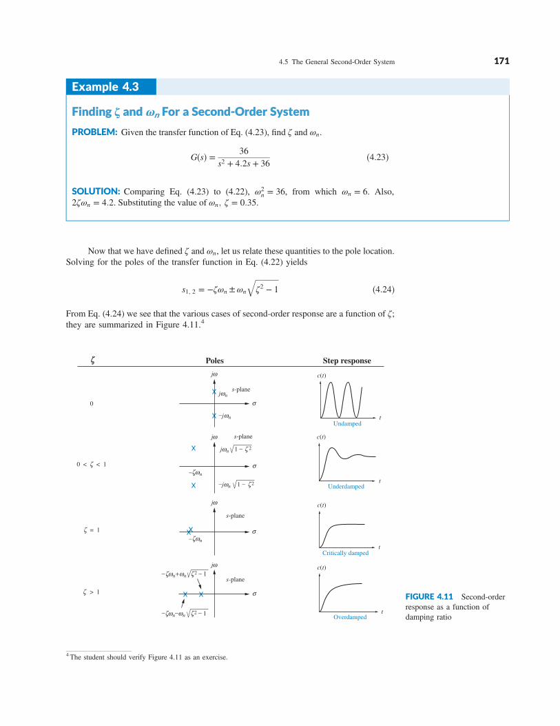
PROBLEM: For each of the systems shown in Figure 4.12, find the value of ζ and report
the kind of response expected.
SOLUTION: First match the form of these systems to the forms shown in Eqs. (4.16) and
(4.22). Since a � 2ζωn and ωn �ffiffiffi
bp
,
ζ � a
2ffiffiffi
bp �4.25�
Using the values of a and b from each of the systems of Figure 4.12, we find
ζ � 1:155 for system (a), which is thus overdamped, since ζ > 1; ζ � 1 for system (b),
which is thus critically damped; and ζ � 0:894 for system (c), which is thus underdamped,
since ζ < 1.
12
(a)
16
(b)
20 C(s)
(c)
s2 + 8s + 12
C(s)C(s)
R(s)
R(s)R(s)
s2 + 8s + 16
s2 + 8s + 20
FIGURE 4.12 Systems for Example 4.4
172 Chapter 4 Time Response

4.6 Underdamped Second-Order Systems
Now that we have generalized the second-order transfer function in terms of ζ and ωn, let us
analyze the step response of an underdamped second-order system. Not only will this
response be found in terms of ζ and ωn, but more specifications indigenous to the
underdamped case will be defined. The underdamped second-order system, a common
model for physical problems, displays unique behavior that must be itemized; a detailed
description of the underdamped response is necessary for both analysis and design. Our first
objective is to define transient specifications associated with underdamped responses. Next
we relate these specifications to the pole location, drawing an association between pole
location and the form of the underdamped second-order response. Finally, we tie the pole
location to system parameters, thus closing the loop: Desired response generates required
system components.
Let us begin by finding the step response for the general second-order system of
Eq. (4.22). The transform of the response, C(s), is the transform of the input times the
transfer function, or
C�s� � ω2n
s�s2 � 2ζωns � ω2n�
� K1
s� K2s � K3
s2 � 2ζωns � ω2n
�4.26�
where it is assumed that ζ < 1 (the underdamped case). Expanding by partial fractions,
using the methods described in Section 2.2, Case 3, yields
C�s� � 1
s�
�s � ζωn� � ζffiffiffiffiffiffiffiffiffiffiffiffi
1 � ζ2p ωn
ffiffiffiffiffiffiffiffiffiffiffiffi
1 � ζ2q
�s � ζωn�2 � ω2n�1 � ζ2� �4.27�
Taking the inverse Laplace transform, which is left as an exercise for the student,
produces
c�t� � 1 � e�ζωnt cosωn
ffiffiffiffiffiffiffiffiffiffiffiffi
1 � ζ2p
t � ζffiffiffiffiffiffiffiffiffiffiffiffi
1 � ζ2p sinωn
ffiffiffiffiffiffiffiffiffiffiffiffi
1 � ζ2q
t
!
� 1 � 1ffiffiffiffiffiffiffiffiffiffiffiffi
1 � ζ2p e�ζωnt cos�ωn
ffiffiffiffiffiffiffiffiffiffiffiffi
1 � ζ2q
t � ϕ��4.28�
where ϕ � tan�1�ζ=ffiffiffiffiffiffiffiffiffiffiffiffi
1 � ζ2p
�.A plot of this response appears in Figure 4.13 for various values of ζ, plotted along a
time axis normalized to the natural frequency. We now see the relationship between the
value of ζ and the type of response obtained: The lower the value of ζ, the more oscillatory
the response. The natural frequency is a time-axis scale factor and does not affect the nature
of the response other than to scale it in time.
We have defined two parameters associated with second-order systems, ζ and ωn.
Other parameters associated with the underdamped response are rise time, peak time,
percent overshoot, and settling time. These specifications are defined as follows (see also
Figure 4.14):
1. Rise time, T r. The time required for the waveform to go from 0.1 of the final value to 0.9
of the final value.
2. Peak time, TP. The time required to reach the first, or maximum, peak.
4.6 Underdamped Second-Order Systems 173

3. Percent overshoot, %OS. The amount that the waveform overshoots the steady-state, or
final, value at the peak time, expressed as a percentage of the steady-state value.
4. Settling time, Ts. The time required for the transient’s damped oscillations to reach and
stay within � 2% of the steady-state value.
Notice that the definitions for settling time and rise time are basically the same as the
definitions for the first-order response. All definitions are also valid for systems of order
higher than 2, although analytical expressions for these parameters cannot be found unless
the response of the higher-order system can be approximated as a second-order system,
which we do in Sections 4.7 and 4.8.
Rise time, peak time, and settling time yield information about the speed of the
transient response. This information can help a designer determine if the speed and
the nature of the response do or do not degrade the performance of the system. For
example, the speed of an entire computer system depends on the time it takes for a hard
drive head to reach steady state and read data; passenger comfort depends in part on the
1 2 3 4 5 6 7 8 9 10 11 12 13 14 15 16 17
0.2
0.4
0.6
0.8
1.0
1.2
1.4
1.6
1.8
c(ωnt)
nt
ζ = .1
0
.2
.4
.5
.6
.8
ω
FIGURE 4.13 Second-order underdamped responses for damping ratio values
Tr Tp Ts
t
0.1c.nal
0.9c.nal
0.98c.nal
c.nal
1.02c.nal
cmax
c(t)
FIGURE 4.14 Second-order underdamped response specifications
174 Chapter 4 Time Response

suspension system of a car and the number of oscillations it goes through after hitting
a bump.
We now evaluate Tp, %OS, and T s as functions of ζ and ωn. Later in this chapter we
relate these specifications to the location of the system poles. A precise analytical expression
for rise time cannot be obtained; thus, we present a plot and a table showing the relationship
between ζ and rise time.
Evaluation of TpTp is found by differentiating c(t) in Eq. (4.28) and finding the first zero crossing after t � 0.
This task is simplified by “differentiating” in the frequency domain by using Item 7 of
Table 2.2. Assuming zero initial conditions and using Eq. (4.26), we get
ℒ� _c�t�� � sC�s� � ω2n
s2 � 2ζωns � ω2n
�4.29�
Completing squares in the denominator, we have
ℒ� _c�t�� � ω2n
�s � ζωn�2 � ω2n�1 � ζ2� �
ωnffiffiffiffiffiffiffiffiffiffiffiffi
1 � ζ2p ωn
ffiffiffiffiffiffiffiffiffiffiffiffi
1 � ζ2q
�s � ζωn�2 � ω2n�1 � ζ2� �4.30�
Therefore,
_c�t� � ωnffiffiffiffiffiffiffiffiffiffiffiffi
1 � ζ2p e�ζωntsinωn
ffiffiffiffiffiffiffiffiffiffiffiffi
1 � ζ2q
t �4.31�
Setting the derivative equal to zero yields
ωn
ffiffiffiffiffiffiffiffiffiffiffiffi
1 � ζ2q
t � nπ �4.32�or
t � nπ
ωn
ffiffiffiffiffiffiffiffiffiffiffiffi
1 � ζ2p �4.33�
Each value of n yields the time for local maxima or minima. Letting n � 0 yields t � 0, the
first point on the curve in Figure 4.14 that has zero slope. The first peak, which occurs at the
peak time, Tp, is found by letting n � 1 in Eq. (4.33):
Tp � π
ωn
ffiffiffiffiffiffiffiffiffiffiffiffi
1 � ζ2p �4.34�
Evaluation of %OSFrom Figure 4.14 the percent overshoot, %OS, is given by
%OS � cmax � cfinal
cfinal� 100 �4.35�
The term cmax is found by evaluating c(t) at the peak time, c(Tp). Using Eq. (4.34) for Tp and
substituting into Eq. (4.28) yields
cmax � c �Tp� � 1 � e��ζπ=ffiffiffiffiffiffiffiffi
1�ζ2p
� cos π � ζffiffiffiffiffiffiffiffiffiffiffiffi
1 � ζ2p sin π
!
� 1 � e��ζπ=ffiffiffiffiffiffiffiffi
1�ζ2p
��4.36�
For the unit step used for Eq. (4.28),
cfinal � 1 �4.37�
4.6 Underdamped Second-Order Systems 175

Substituting Eqs. (4.36) and (4.37) into Eq. (4.35), we finally obtain
%OS � e��ζπ=ffiffiffiffiffiffiffiffi
1�ζ2p
� � 100 �4.38�
Notice that the percent overshoot is a function only of the damping ratio, ζ.
Whereas Eq. (4.38) allows one to find%OS given ζ, the inverse of the equation allows
one to solve for ζ given %OS. The inverse is given by
ζ � �ln �%OS=100�ffiffiffiffiffiffiffiffiffiffiffiffiffiffiffiffiffiffiffiffiffiffiffiffiffiffiffiffiffiffiffiffiffiffiffiffiffiffiffi
π2 � ln2�%OS=100�q �4.39�
The derivation of Eq. (4.39) is left as an exercise for the student. Equation (4.38) (or,
equivalently, (4.39)) is plotted in Figure 4.15.
Evaluation of TsIn order to find the settling time, we must find the time for which c(t) in Eq. (4.28) reaches
and stays within � 2% of the steady-state value, cfinal. Using our definition, the settling time
is the time it takes for the amplitude of the decaying sinusoid in Eq. (4.28) to reach 0.02, or
e�ζωnt1ffiffiffiffiffiffiffiffiffiffiffiffi
1 � ζ2p � 0:02 �4.40�
This equation is a conservative estimate, since we are assuming that
cos�ωn
ffiffiffiffiffiffiffiffiffiffiffiffi
1 � ζ2p
t � ϕ� � 1 at the settling time. Solving Eq. (4.40) for t, the settling time is
Ts � �ln�0:02ffiffiffiffiffiffiffiffiffiffiffiffi
1 � ζ2p
�ζωn
�4.41�
You can verify that the numerator of Eq. (4.41) varies from 3.91 to 4.74 as ζ varies from
0 to 0.9. Let us agree on an approximation for the settling time that will be used for all values
of ζ; let it be
Ts � 4
ζωn
�4.42�
Evaluation of TrA precise analytical relationship between rise time and damping ratio, ζ, cannot be found.
However, using a computer and Eq. (4.28), the rise time can be found.We first designateωnt
0.90.80.70.60.50.40.30.20.10
10
20
30
40
50
60
70
80
90
100
Damping ratio, ζP
erce
nt
over
shoot,
%OS
FIGURE 4.15 Percent
overshoot versus damping ratio
176 Chapter 4 Time Response

as the normalized time variable and select a value for ζ. Using the computer, we solve for the
values of ωnt that yield c�t� � 0:9 and c�t� � 0:1. Subtracting the two values of ωnt yields
the normalized rise time, ωnTr, for that value of ζ. Continuing in like fashion with other
values of ζ, we obtain the results plotted in Figure 4.16.5 Let us look at an example.
0.2 0.3 0.4 0.5 0.6 0.7 0.8 0.90.11.0
1.2
1.4
1.6
1.8
2.0
2.2
2.4
2.6
2.8
3.0
Damping ratio
Damping
ratio
Normalized
rise time
0.1
0.2
0.3
0.4
0.5
0.6
0.7
0.8
0.9
1.104
1.203
1.321
1.463
1.638
1.854
2.126
2.467
2.883
Ris
e ti
me
× N
atura
l fr
equen
cy
FIGURE 4.16 Normalized rise time versus damping ratio for a second-order underdamped response
Example 4.5
Finding Tp , %OS,Ts , and Tr from a Transfer FunctionFinding Tp , %OS,Ts , and Tr from a Transfer Function
PROBLEM: Given the transfer function
G�s� � 100
s2 � 15s � 100�4.43�
find Tp, %OS, T s, and Tr.
SOLUTION: ωn and ζ are calculated as 10 and 0.75, respectively. Now substitute
ζ and ωn into Eqs. (4.34), (4.38), and (4.42) and find, respectively, that Tp � 0:475second, %OS � 2:838, and T s � 0:533 second. Using the table in Figure 4.16, the
normalized rise time is approximately 2.3 seconds. Dividing by ωn yields T r � 0:23second. This problem demonstrates that we can find Tp, %OS, T s, and T r without the
tedious task of taking an inverse Laplace transform, plotting the output response, and
taking measurements from the plot.
Virtual Experiment 4.2
Second-Order
System Response
Put theory into practice studying
the effect that natural frequency
and damping ratio have on
controlling the speed response
of the Quanser Linear Servo in
LabVIEW. This concept is
applicable to automobile cruise
controls or speed controls of
subways or trucks.
Virtual experiments are found
on Learning Space.
5 Figure 4.16 can be approximated by the following polynomials: ωnT r � 1:76ζ3 � 0:417ζ2 � 1:039ζ � 1 (maximum
error less than 12% for 0 < ζ < 0:9), and ζ � 0:115�ωnT r�3 � 0:883�ωnT r�2 � 2:504�ωnT r� � 1:738 (maximum error
less than 5% for 0:1 < ζ < 0:9). The polynomials were obtained using MATLAB’s polyfit function.
4.6 Underdamped Second-Order Systems 177

We now have expressions that relate peak time, percent overshoot,
and settling time to the natural frequency and the damping ratio. Now let
us relate these quantities to the location of the poles that generate these
characteristics.
The pole plot for a general, underdamped second-order system,
previously shown in Figure 4.11, is reproduced and expanded in
Figure 4.17 for focus. We see from the Pythagorean theorem that the
radial distance from the origin to the pole is the natural frequency,ωn, and
the cos θ � ζ.
Now, comparing Eqs. (4.34) and (4.42) with the pole location, we
evaluate peak time and settling time in terms of the pole location. Thus,
Tp � π
ωn
ffiffiffiffiffiffiffiffiffiffiffiffi
1 � ζ2p � π
ωd
�4.44�
T s � 4
ζωn
� π
σd�4.45�
where ωd is the imaginary part of the pole and is called the damped frequency of
oscillation, and σd is the magnitude of the real part of the pole and is the exponential
damping frequency.
Equation (4.44) shows that Tp is inversely proportional to the imaginary part of
the pole. Since horizontal lines on the s-plane are lines of constant imaginary value, they
are also lines of constant peak time. Similarly, Eq. (4.45) tells us that settling time is
inversely proportional to the real part of the pole. Since vertical lines on the s-plane are
lines of constant real value, they are also lines of constant settling time. Finally, since
ζ � cos θ, radial lines are lines of constant ζ. Since percent overshoot is only a function
of ζ, radial lines are thus lines of constant percent overshoot, %OS. These concepts
are depicted in Figure 4.18, where lines of constant Tp, T s, and %OS are labeled on the
s-plane.
At this point, we can understand the significance of Figure 4.18 by examining the
actual step response of comparative systems. Depicted in Figure 4.19(a) are the step
responses as the poles are moved in a vertical direction, keeping the real part the same.
n dσ
ωn
θ
ζ–
–jω 1 – ζ2n
jω 1 – ζ 2n
σ
jω
s-plane
+
= –
= –jωd
= jωd
ω
FIGURE 4.17 Pole plot for an underdamped
second-order system
%OS2
%OS1
jω
s-plane
Ts2Ts1
Tp2
Tp1
σ
FIGURE 4.18 Lines of
constant peak time, Tp, settling
time, T s, and percent overshoot,
%OS. Note: T s2 < Ts1 ;
Tp2 < Tp1; %OS1 < %OS2.
178 Chapter 4 Time Response

As the poles move in a vertical direction, the frequency increases, but the envelope remains
the same since the real part of the pole is not changing. The figure shows a constant
exponential envelope, even though the sinusoidal response is changing frequency. Since all
curves fit under the same exponential decay curve, the settling time is virtually the same for
all waveforms. Note that as overshoot increases, the rise time decreases.
Let us move the poles to the right or left. Since the imaginary part is now
constant, movement of the poles yields the responses of Figure 4.19(b). Here the
frequency is constant over the range of variation of the real part. As the poles move to
the left, the response damps out more rapidly, while the frequency remains the same.
Notice that the peak time is the same for all waveforms because the imaginary part
remains the same.
Moving the poles along a constant radial line yields the responses shown in
Figure 4.19(c). Here the percent overshoot remains the same. Notice also that the responses
look exactly alike, except for their speed. The farther the poles are from the origin, the more
rapid the response.
We conclude this section with some examples that demonstrate the relationship
between the pole location and the specifications of the second-order underdamped
response. The first example covers analysis. The second example is a simple design problem
consisting of a physical systemwhose component valueswewant to design tomeet a transient
Frequency the same
12
t
c(t)
Polemotion
t
c(t)
Polemotion
t
c(t)
Same overshoot
Polemotion
s-plane
s-plane
s-plane
(a)
(c)
jω
jω
jω
(b)
12
3
3
2
1
12
12
1
2
3
12
3
1
2
3
Envelope the same
1
2
3
σ
σ
σ
FIGURE 4.19 Step responses
of second-order underdamped
systems as poles move: a. with
constant real part; b. with
constant imaginary part; c. with
constant damping ratio
4.6 Underdamped Second-Order Systems 179

response specification. An animation PowerPoint presentation (PPT) demonstrating
second-order principles is available for instructors at www.wiley.com/college/nise. See
Second-Order Step Response.
Example 4.6
Finding Tp , %OS, and Ts from Pole LocationFinding Tp , %OS, and Ts from Pole Location
PROBLEM: Given the pole plot shown in Figure 4.20, findζ; ωn; Tp;%OS, and T s.
SOLUTION: The damping ratio is given by ζ � cos θ � cos�arctan �7=3�� �0:394. The natural frequency,ωn, is the radial distance from the origin to the
pole, or ωn �ffiffiffiffiffiffiffiffiffiffiffiffiffiffiffi
72 � 32p
� 7:616. The peak time is
Tp �π
ωd
� π7� 0:449 second �4.46�
The percent overshoot is
%OS � e��ζπ=ffiffiffiffiffiffiffiffi
1�ζ2p
� � 100 � 26% �4.47�
The approximate settling time is
Ts �4
σd� 4
3� 1:333 seconds �4.48�
Students who are using MATLAB should now run ch4p1 in Appendix B.You will learn how to generate a second-order polynomial from twocomplex poles as well as extract and use the coefficients of thepolynomial to calculate Tp, %OS, and Ts. This exercise uses MATLABto solve the problem in Example 4.6.
s-plane
θ
d
j7 = jωd
–j7 = –jωd
jω
3– = –σ
σ
FIGURE 4.20 Pole plot for Example 4.6
Example 4.7
Transient Response Through Component DesignTransient Response Through Component Design
PROBLEM: Given the system shown in Figure 4.21, find J and D to yield 20%
overshoot and a settling time of 2 seconds for a step input of torque T(t).
J
D
T(t) θ
K = 5 N-m/rad
(t)
FIGURE 4.21 Rotational mechanical system for Example 4.7
180 Chapter 4 Time Response

Second-Order Transfer Functions via TestingJust as we obtained the transfer function of a first-order system experimentally, we can do
the same for a system that exhibits a typical underdamped second-order response. Again, we
can measure the laboratory response curve for percent overshoot and settling time, from
which we can find the poles and hence the denominator. The numerator can be found, as in
the first-order system, from a knowledge of the measured and expected steady-state values.
A problem at the end of the chapter illustrates the estimation of a second-order transfer
function from the step response.
SOLUTION: First, the transfer function for the system is
G�s� � 1=J
s2 � D
Js � K
J
�4.49�
From the transfer function,
ωn �ffiffiffiffi
K
J
r
�4.50�
and
2ζωn �D
J�4.51�
But, from the problem statement,
Ts � 2 � 4
ζωn
�4.52�
or ζωn � 2. Hence,
2ζωn � 4 � D
J�4.53�
Also, from Eqs. (4.50) and (4.52),
ζ � 4
2ωn
� 2
ffiffiffiffi
J
K
r
�4.54�
From Eq. (4.39), a 20% overshoot implies ζ � 0:456. Therefore, from Eq. (4.54),
ζ � 2
ffiffiffiffi
J
K
r
� 0:456 �4.55�
Hence,
J
K� 0:052 �4.56�
From the problem statement, K � 5 N-m/rad. Combining this value with Eqs. (4.53) and
(4.56), D= 1.04 N-m-s/rad, and J � 0:26 kg-m2.
4.6 Underdamped Second-Order Systems 181

Now that we have analyzed systems with two poles, how does the addition of another
pole affect the response? We answer this question in the next section.
4.7 System Response with Additional Poles
In the last section, we analyzed systems with one or two poles. It must be emphasized that
the formulas describing percent overshoot, settling time, and peak time were derived
only for a system with two complex poles and no zeros. If a system such as that shown in
Figure 4.22 has more than two poles or has zeros, we cannot use the formulas to calculate the
performance specifications that we derived. However, under certain conditions, a system
with more than two poles or with zeros can be approximated as a second-order system that
has just two complex dominant poles. Once we justify this approximation, the formulas for
percent overshoot, settling time, and peak time can be applied to these higher-order systems
by using the location of the dominant poles. In this section, we investigate the effect of an
additional pole on the second-order response. In the next section, we analyze the effect of
adding a zero to a two-pole system.
Let us now look at the conditions that would have to exist in order to approximate the
behavior of a three-pole system as that of a two-pole system. Consider a three-pole system
with complex poles and a third pole on the real axis. Assuming that the complex poles are at
�ζωn � jωn
ffiffiffiffiffiffiffiffiffiffiffiffi
1 � ζ2p
and the real pole is at �αr, the step response of the system can be
determined from a partial-fraction expansion. Thus, the output transform is
C�s� � A
s� B�s � ζωn� � Cωd
�s � ζωn�2 � ω2d
� D
s � αr�4.57�
or, in the time domain,
c�t� � Au�t� � e�ζωnt�B cosωdt � C sin ωdt� � De�αr t �4.58�The component parts of c(t) are shown in Figure 4.23 for three cases of αr. For Case I,
αr � αr1 and is not much larger than ζωn; for Case II, αr � αr2 and is much larger than ζωn;
and for Case III, αr � ∞:
Skill-Assessment Exercise 4.5
PROBLEM: Find ζ; ωn; T s; Tp; Tr, and %OS for a system whose transfer
function is G�s� � 361
s2 � 16s � 361.
ANSWERS:
ζ � 0:421; ωn � 19; Ts � 0:5 s; Tp � 0:182 s; T r � 0:079 s; and%OS � 23:3%:
The complete solution is located at www.wiley.com/college/nise.
TryIt 4.1
Use the following MATLAB
statements to calculate the
answers to Skill-Assessment
Exercise 4.5. Ellipses mean
code continues on next line.
numg=361;deng=[1 16 361];omegan=sqrt(deng(3).../deng(1))
zeta=(deng(2)/deng(1)).../(2*omegan)
Ts=4/(zeta*omegan)Tp=pi/(omegan*sqrt...(1-zeta^2))
pos=100*exp(-zeta*...pi/sqrt(1-zeta^2))
Tr=(1.768*zeta^3 -...0.417*zeta^2+1.039*...zeta+1)/omegan
182 Chapter 4 Time Response

FIGURE 4.22 Robot follows
input commands from a human
trainer
Au(t) + e– nt(B cos d t + C sin d t)
α– r1– n
p2
p1
p3s-plane
Case I Case II
(a)
Case III
α– r2ζ– n
p2
p1
p3
ζ– n
p2
p1
s-plane s-plane
II
Case I
III
II
Case I
Response
Time
(b)
0
jω jω jω
De–αrit
ζω ω ω
ζω ω ω
σ σ σ
FIGURE 4.23 Component
responses of a three-pole
system: a. pole plot;
b. component responses:
Nondominant pole is near
dominant second-order
pair (Case I), far from the
pair (Case II), and at infinity
(Case III)
4.7 System Response with Additional Poles 183

Let us direct our attention to Eq. (4.58) and Figure 4.23. If αr � ζωn (Case II), the
pure exponential will die out much more rapidly than the second-order underdamped step
response. If the pure exponential term decays to an insignificant value at the time of the
first overshoot, such parameters as percent overshoot, settling time, and peak time will be
generated by the second-order underdamped step response component. Thus, the total
response will approach that of a pure second-order system (Case III).
If αr is not much greater than ζωn (Case I), the real pole’s transient response will not
decay to insignificance at the peak time or settling time generated by the second-order pair.
In this case, the exponential decay is significant, and the system cannot be represented as a
second-order system.
The next question is, How much farther from the dominant poles does the third pole
have to be for its effect on the second-order response to be negligible? The answer of course
depends on the accuracy for which you are looking. However, this book assumes that the
exponential decay is negligible after five time constants. Thus, if the real pole is five times
farther to the left than the dominant poles, we assume that the system is represented by its
dominant second-order pair of poles.
What about the magnitude of the exponential decay? Can it be so large that its
contribution at the peak time is not negligible? We can show, through a partial-fraction
expansion, that the residue of the third pole, in a three-pole system with dominant
second-order poles and no zeros, will actually decrease in magnitude as the third pole is
moved farther into the left half-plane. Assume a step response, C(s), of a three-pole
system:
C�s� �bc
s�s2 � as � b��s � c��A
s�
Bs � C
s2 � as � b�
D
s � c�4.59�
where we assume that the nondominant pole is located at �c on the real axis and that the
steady-state response approaches unity. Evaluating the constants in the numerator of
each term,
A � 1; B �ca � c2
c2 � b � ca(4.60a)
C �ca2 � c2a � bc
c2 � b � ca; D �
�b
c2 � b � ca(4.60b)
As the nondominant pole approaches ∞; or c®∞,
A � 1; B � �1; C � �a; D � 0 �4.61�
Thus, for this example, D, the residue of the nondominant pole and its response, becomes
zero as the nondominant pole approaches infinity.
The designer can also choose to forgo extensive residue analysis, since all system
designs should be simulated to determine final acceptance. In this case, the control systems
engineer can use the “five times” rule of thumb as a necessary but not sufficient condition to
increase the confidence in the second-order approximation during design, but then simulate
the completed design.
Let us look at an example that compares the responses of two different three-pole
systems with that of a second-order system.
184 Chapter 4 Time Response

Example 4.8
Comparing Responses of Three-Pole SystemsComparing Responses of Three-Pole Systems
PROBLEM: Find the step response of each of the transfer functions shown in Eqs. (4.62)
through (4.64) and compare them.
T1�s� �24:542
s2 � 4s � 24:542(4.62)
T2�s� �245:42
�s � 10��s2 � 4s � 24:542��4.63�
T3�s� �73:626
�s � 3��s2 � 4s � 24:542��4.64�
SOLUTION: The step response, Ci�s�, for the transfer function, T i�s�, can be found by
multiplying the transfer function by 1/s, a step input, and using partial-fraction expansion
followed by the inverse Laplace transform to find the response, ci�t�. With the details left
as an exercise for the student, the results are
c1�t� � 1 � 1:09e�2tcos �4:532t � 23:8°� �4.65�
c2�t� � 1 � 0:29e�10t � 1:189e�2tcos �4:532t � 53:34°� �4.66�
c3�t� � 1 � 1:14e�3t � 0:707e�2tcos �4:532t � 78:63°� �4.67�
The three responses are plotted in Figure 4.24. Notice that c2�t�, with its third pole at
�10 and farthest from the dominant poles, is the better approximation of c1�t�, the pure
second-order system response; c3�t�, with a third pole close to the dominant poles,
yields the most error.
1.4
1.2
1.0
0.8
0.6
0.4
0.2
0 0.5 2.0 2.5 3.0
Time (seconds)
Norm
aliz
ed r
esponse
c1(t)
c2(t)
c3(t)
1.0 1.5
FIGURE 4.24 Step responses of system T1�s�, system T2�s�, and system T3�s�
4.7 System Response with Additional Poles 185

4.8 System Response with Zeros
Now that we have seen the effect of an additional pole, let us add a zero to the second-order
system. In Section 4.2, we saw that the zeros of a response affect the residue, or amplitude,
of a response component but do not affect the nature of the response—exponential, damped
sinusoid, and so on. In this section, we add a real-axis zero to a two-pole system. The zero
Students who are using MATLAB should now run ch4p2 in Appendix B.You will learn how to generate a step response for a transferfunction and how to plot the response directly or collect thepoints for future use. The example shows how to collect the pointsand then use them to create a multiple plot, title the graph, andlabel the axes and curves to produce the graph in Figure 4.24 tosolve Example 4.8.System responses can alternately be obtained using Simulink.Simulink is a software package that is integrated with MATLABto provide a graphical user interface (GUI) for defining systemsand generating responses. The reader is encouraged to studyAppendix C, which contains a tutorial on Simulink as well as someexamples. One of the illustrative examples, Example C.1, solvesExample 4.8 using Simulink.Another method to obtain systems responses is through the use ofMATLAB's LTI Viewer. An advantage of the LTI Viewer is that itdisplays the values of settling time, peak time, rise time, maximumresponse, and the final value on the step response plot. The readeris encouraged to study Appendix E at www.wiley.com/college/nise,which contains a tutorial on the LTI Viewer as well as someexamples. Example E.1 solves Example 4.8 using the LTI Viewer.
Skill-Assessment Exercise 4.6
PROBLEM: Determine the validity of a second-order approximation for each of these
two transfer functions:
a. G�s� �700
�s � 15��s2 � 4s � 100�
b. G�s� �360
�s � 4��s2 � 2s � 90�
ANSWERS:
a. The second-order approximation is valid.
b. The second-order approximation is not valid.
The complete solution is located at www.wiley.com/college/nise.
TryIt 4.2
Use the following MATLAB
and Control System Toolbox
statements to investigate the
effect of the additional pole
in Skill-Assessment
Exercise 4.6(a). Move the
higher-order pole originally
at �15 to other values by
changing “a” in the code.
a=15numga=100*a;denga=conv([1 a],...[1 4 100]);Ta=tf (numga,denga);numg=100;deng=[1 4 100];T=tf (numg,deng);step(Ta,'.',T,'-')
186 Chapter 4 Time Response

will be added first in the left half-plane and then in the right half-plane and its effects noted
and analyzed. We conclude the section by talking about pole-zero cancellation.
Starting with a two-pole system with poles at ��1� j 2:828�, we consecutively add
zeros at �3, �5, and �10. The results, normalized to the steady-state value, are plotted in
Figure 4.25.We can see that the closer the zero is to the dominant poles, the greater its effect on
the transient response. As the zero moves away from the dominant poles, the response
approaches that of the two-pole system. This analysis can be reasoned via the partial-fraction
expansion. If we assume a group of poles and a zero far from the poles, the residue of each pole
will be affected the same by the zero. Hence, the relative amplitudes remain appreciably the
same. For example, assume the partial-fraction expansion shown in Eq. (4.68):
T�s� ��s � a�
�s � b��s � c��
A
s � b�
B
s � c
���b � a�=��b � c�
s � b���c � a�=��c � b�
s � c�4.68�
If the zero is far from the poles, then a is large compared to b and c, and
T�s�≈ a1=��b � c�
s � b�1=��c � b�
s � c
!
�a
�s � b��s � c��4.69�
Hence, the zero looks like a simple gain factor and does not change the relative amplitudes of
the components of the response.
Another way to look at the effect of a zero, which is more general, is as follows
(Franklin, 1991): Let C(s) be the response of a system, T(s), with unity in the numerator. If
we add a zero to the transfer function, yielding �s � a�T�s�, the Laplace transform of the
response will be
�s � a�C�s� � sC�s� � aC�s� �4.70�
Thus, the response of a system with a zero consists of two parts: the derivative of the original
response and a scaled version of the original response. If a, the negative of the zero, is very
large, the Laplace transform of the response is approximately aC(s), or a scaled version of
the original response. If a is not very large, the response has an additional component
consisting of the derivative of the original response. As a becomes smaller, the derivative
term contributes more to the response and has a greater effect. For step responses, the
derivative is typically positive at the start of a step response. Thus, for small values of a,
we can expect more overshoot in second-order systems because the derivative term will be
additive around the first overshoot. This reasoning is borne out by Figure 4.25.
TryIt 4.3
Use the following MATLAB and
Control System Toolbox
statements to generate
Figure 4.25.
deng=[1 2 9];Ta=tf([1 3]*9/3,deng);Tb=tf([1 5]*9/5,deng);Tc=tf([1 10]*9/10,deng);T=tf(9,deng);step(T,Ta,Tb,Tc)text(0.5,0.6,'no zero')text(0.4,0.7,...'zero at �10')text(0.35,0.8,...'zero at �5')text(0.3,0.9,'zero at �3')
1.4
1.2
1.0
0.8
0.6
0.4
0.2
0 2.0 4.0 6.0
Time (seconds)
1.6
zero at –3
zero at –5
zero at –10
no zero
No
rmal
ized
c(t
)
FIGURE 4.25 Effect of adding a zero to a two-pole system
4.8 System Response with Zeros 187
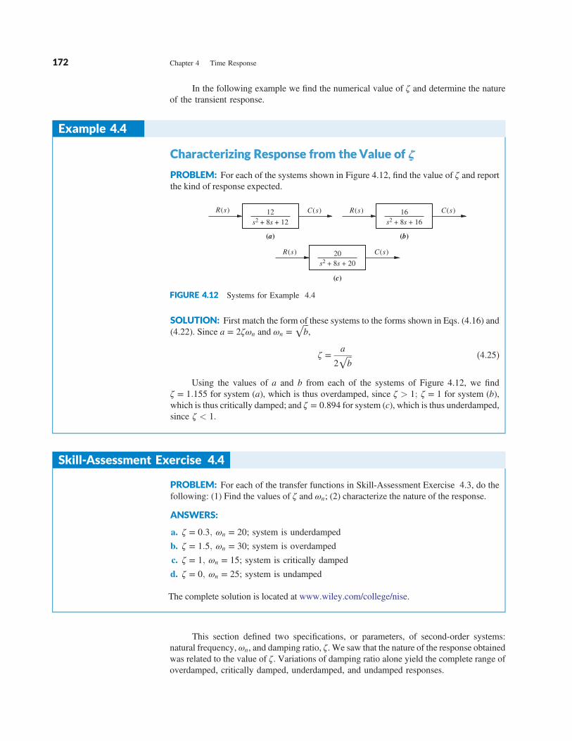
An interesting phenomenon occurs if a is negative, placing the zero in the right
half-plane. From Eq. (4.70) we see that the derivative term, which is typically positive
initially, will be of opposite sign from the scaled response term. Thus, if the derivative term,
sC(s), is larger than the scaled response, aC(s), the response will initially follow the
derivative in the opposite direction from the scaled response. The result for a second-order
system is shown in Figure 4.26, where the sign of the input was reversed to yield a positive
steady-state value. Notice that the response begins to turn toward the negative direction even
though the final value is positive. A system that exhibits this phenomenon is known as a
nonminimum-phase system. If a motorcycle or airplane was a nonminimum-phase system, it
would initially veer left when commanded to steer right.
Let us now look at an example of an electrical nonminimum-phase network.
1.5
1.0 3.0 4.0 5.0
Time (seconds)
c(t)
–0.5
2.0 6.0
1.0
0.5
0
FIGURE 4.26 Step response of a nonminimum-phase system
Example 4.9
Transfer Function of a Nonminimum-PhaseSystemTransfer Function of a Nonminimum-PhaseSystem
PROBLEM:
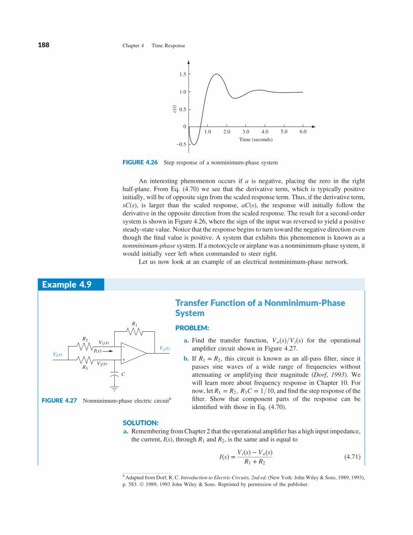
a. Find the transfer function, Vo�s�=V i�s� for the operational
amplifier circuit shown in Figure 4.27.
b. If R1 � R2, this circuit is known as an all-pass filter, since it
passes sine waves of a wide range of frequencies without
attenuating or amplifying their magnitude (Dorf, 1993). We
will learn more about frequency response in Chapter 10. For
now, let R1 � R2; R3C � 1=10, and find the step response of thefilter. Show that component parts of the response can be
identified with those in Eq. (4.70).
SOLUTION:a. Remembering fromChapter 2 that the operational amplifier has a high input impedance,
the current, I(s), through R1 and R2, is the same and is equal to
I�s� �V i�s� � Vo�s�
R1 � R2
�4.71�
Vi(s)
R2V1(s)
R1
I(s)
R3
V2(s)
Vo(s)
C
+
–
FIGURE 4.27 Nonminimum-phase electric circuit6
6Adapted from Dorf, R. C. Introduction to Electric Circuits, 2nd ed. (New York: JohnWiley & Sons, 1989, 1993),
p. 583. 1989, 1993 John Wiley & Sons. Reprinted by permission of the publisher.
188 Chapter 4 Time Response
Also,
Vo�s� � A V2�s� � V1�s�� � �4.72�
But,
V1�s� � I�s�R1 � Vo�s� �4.73�
Substituting Eq. (4.71) into (4.73),
V1�s� �1
R1 � R2
R1V i�s� � R2V0 �s�� � �4.74�
Using voltage division,
V2�s� � V i�s�1=Cs
R3 �1
Cs
�4.75�
Substituting Eqs. (4.74) and (4.75) into Eq. (4.72) and simplifying yields
Vo�s�
V i�s��
A�R2 � R1R3Cs�
�R3Cs � 1��R1 � R2�1 � A���4.76�
Since the operational amplifier has a large gain,A, let A approach infinity. Thus, after
simplification
Vo�s�
V i�s��R2 � R1R3Cs
R2R3Cs � R2
� �R1
R2
s �R2
R1R3C
" #
s �1
R3C
" # �4.77�
b. Letting R1 � R2 and R3C � 1=10,
Vo�s�
V i�s��
s �1
R3C
" #
s �1
R3C
" # � ��s � 10�
�s � 10��4.78�
For a step input, we evaluate the response as suggested by Eq. (4.70):
C�s� � ��s � 10�
s�s � 10�� �
1
s � 10� 10
1
s�s � 10�� sCo�s� � 10Co�s� �4.79�
where
Co�s� � �1
s�s � 10��4.80�
is the Laplace transform of the response without a zero. Expanding Eq. (4.79) into
partial fractions,
C�s� � �1
s � 10� 10
1
s�s � 10�� �
1
s � 10�1
s�
1
s � 10�1
s�
2
s � 10�4.81�
4.8 System Response with Zeros 189

We conclude this section by talking about pole-zero cancellation and its effect on our
ability to make second-order approximations to a system. Assume a three-pole system with
a zero as shown in Eq. (4.85). If the pole term, �s � p3�, and the zero term, �s � z�, cancel out,
we are left with
T�s� �K�s � z�
�s � p3��s2 � as � b�
�4.85�
as a second-order transfer function. From another perspective, if the zero at �z is very close
to the pole at �p3, then a partial-fraction expansion of Eq. (4.85) will show that the residue
of the exponential decay is much smaller than the amplitude of the second-order response.
Let us look at an example.
or the response with a zero is
c�t� � �e�10t � 1 � e�10t � 1 � 2e�10t �4.82�
Also, from Eq. (4.80),
Co�s� � �1=10
s�
1=10
s � 10�4.83�
or the response without a zero is
co�t� � �1
10�
1
10e�10t �4.84�
The normalized responses are plotted in Figure 4.28. Notice the immediate reversal
of the nonminimum-phase response, c(t).
–0.5
–1.0
0.1 0.2 0.3 0.4 0.5
Time (seconds)
Res
ponse
–10co(t)
c (t)
1.0
0.5
00
FIGURE 4.28 Step response of the nonminimum-phase network of Figure 4.27 (c(t)) and
normalized step response of an equivalent network without the zero (�10 co�t�)
Example 4.10
Evaluating Pole-Zero Cancellation Using ResiduesEvaluating Pole-Zero Cancellation Using Residues
PROBLEM: For each of the response functions in Eqs. (4.86) and (4.87), determine
whether there is cancellation between the zero and the pole closest to the zero. For any
function for which pole-zero cancellation is valid, find the approximate response.
C1�s� �26:25�s � 4�
s�s � 3:5��s � 5��s � 6��4.86�
190 Chapter 4 Time Response

In this section, we have examined the effects of additional transfer function poles and
zeros upon the response. In the next section we add nonlinearities of the type discussed in
Section 2.10 and see what effects they have on system response.
C2�s� �26:25�s � 4�
s�s � 4:01��s � 5��s � 6��4.87�
SOLUTION: The partial-fraction expansion of Eq. (4.86) is
C1�s� �1
s�
3:5
s � 5�
3:5
s � 6�
1
s � 3:5�4.88�
The residue of the pole at �3.5, which is closest to the zero at �4, is equal to 1 and is not
negligible compared to the other residues. Thus, a second-order step response approxi-
mation cannot be made for C1�s�. The partial-fraction expansion for C2�s� is
C2�s� �0:87
s�
5:3
s � 5�
4:4
s � 6�
0:033
s � 4:01�4.89�
The residue of the pole at �4.01, which is closest to the zero at �4, is equal to 0.033, about
two orders of magnitude below any of the other residues. Hence, we make a second-order
approximation by neglecting the response generated by the pole at �4.01:
C2�s�≈0:87
s�
5:3
s � 5�
4:4
s � 6�4.90�
and the response c2�t� is approximately
c2�t�≈ 0:87 � 5:3e�5t � 4:4e�6t �4.91�
TryIt 4.4
Use the following MATLAB
and Symbolic Math Toolbox
statements to evaluate the effect
of higher-order poles by finding
the component parts of the time
response of c1�t� and c2�t� in
Example 4.10.
syms sC1=26.25*(s+4)/...(s*(s+3.5)*...(s+5)*(s+6));
C2=26.25*(s+4)/...(s*(s+4.01)*...(s+5)*(s+6));
c1=ilaplace(C1);'c1'c1=vpa(c1,3)c2=ilaplace(C2);'c2'c2=vpa(c2,3)
Skill-Assessment Exercise 4.7
PROBLEM: Determine the validity of a second-order step-response approximation for
each transfer function shown below.
a. G�s� �185:71�s � 7�
�s � 6:5��s � 10��s � 20�
b. G�s� �197:14�s � 7�
�s � 6:9��s � 10��s � 20�
ANSWERS:
a. A second-order approximation is not valid.
b. A second-order approximation is valid.
The complete solution is located at www.wiley.com/college/nise.
4.8 System Response with Zeros 191

4.9 Effects of Nonlinearities upon Time Response
In this section, we qualitatively examine the effects of nonlinearities upon the time response
of physical systems. In the following examples, we insert nonlinearities, such as saturation,
dead zone, and backlash, as shown in Figure 2.46, into a system to show the effects of these
nonlinearities upon the linear responses.
The responses were obtained using Simulink, a simulation software package that is
integrated with MATLAB to provide a graphical user interface (GUI). Readers who would
like to learn how to use Simulink to generate nonlinear responses should consult the
Simulink tutorial in Appendix C. Simulink block diagrams are included with all responses
that follow.
Let us assume the motor and load from the Antenna Control Case Study of Chapter 2
and look at the load angular velocity, ωo�s�, where ωo�s� � 0:1 sθm�s� � 0:2083 Ea�s�=�s � 1:71� from Eq. (2.208). If we drive the motor with a step input through an amplifier of
unity gain that saturates at � 5 volts, Figure 4.29 shows that the effect of amplifier saturation
is to limit the obtained velocity.
Load
angula
r vel
oci
ty (
rad/s
econd)
0 2 4 6 8 100
0.5
1
1.5
With saturation
Without saturation
Time (seconds)
(a)
Step
10 volts
Saturation
±5 voltsMotor, load,
& gears
Mux Scope
Motor, load,
& gears(b)
0.2083
s + 1.71
0.2083
s + 1.71
FIGURE 4.29 a. Effect of amplifier saturation on load angular velocity response; b. Simulink block
diagram
192 Chapter 4 Time Response

The effect of dead zone on the output shaft driven by a motor and gears is shown in Figure
4.30. Here we once again assume the motor, load, and gears from Antenna Control Case
Study of Chapter 2. Dead zone is present when the motor cannot respond to small voltages.
The motor input is a sinusoidal waveform chosen to allow us to see the effects of dead zone
vividly. The response begins when the input voltage to the motor exceeds a threshold. We
notice a lower amplitude when dead zone is present.
The effect of backlash on the output shaft driven by a motor and gears is shown in
Figure 4.31. Again we assume the motor, load, and gears from the Antenna Control Case
Study of Chapter 2. The motor input is again a sinusoidal waveform, which is chosen to allow
us to see vividly the effects of backlash in the gears driven by themotor. As themotor reverses
direction, the output shaft remains stationary while the motor begins to reverse. When the
gearsfinally connect, the output shaft itself begins to turn in the reverse direction. The resulting
response is quite different from the linear response without backlash.
0 5 10 15 20 250
0.2
0.4
0.6
0.8
1
1.2
Time (seconds)
(a)
Load angular displacement (radians)
Without dead zone
With dead zone
MuxScope
Sine wave
Amplitude = 5
Frequency = 1 rad/s
Dead zone
–2 to +2
(b)
Motor, load,
& gears
Motor, load,
& gears
Integrator
Integrator
1s
1s
0.2083
s + 1.71
0.2083
s + 1.71
FIGURE 4.30 a. Effect of dead zone on load angular displacement response; b. Simulink block
diagram
4.9 Effects of Nonlinearities upon Time Response 193

Now that we have seen the effects of nonlinearities on the time response, let us return
to linear systems. Our coverage so far for linear systems has dealt with finding the time
response by using the Laplace transform in the frequency domain. Another way to solve for
the response is to use state-space techniques in the time domain. This topic is the subject of
the next two sections.
4.10 Laplace Transform Solution of State Equations
In Chapter 3, systems were modeled in state space, where the state-space representation
consisted of a state equation and an output equation. In this section, we use the Laplace
transform to solve the state equations for the state and output vectors.
0 5 10 15 20 250
0.05
0.1
0.15
0.2
0.25
Time (seconds)
(a)
Load angular displacement (radians)
With backlash
Without backlash
(b)
0.2083
s + 1.71
0.2083
s + 1.71
Motor, load,and gears
Motor, load,and gears
Scope
1s
1s
Integrator
Integrator
Sine waveAmplitude = 5
Frequency = 1 rad/s
Backlashdeadband width
0.15 Mux
FIGURE 4.31 a.Effect of backlash on load angular displacement response;b. Simulink blockdiagram
Skill-Assessment Exercise 4.8
PROBLEM: Use MATLAB's Simulink to reproduce Figure 4.31.ANSWER: See Figure 4.31.
194 Chapter 4 Time Response

Consider the state equation
_x � Ax � Bu �4.92�
and the output equation
y � Cx � Du �4.93�
Taking the Laplace transform of both sides of the state equation yields
sX�s� � x�0� � AX�s� � BU�s� �4.94�
In order to separateX(s), replace sX(s) with sIX(s), where I is an n � n identity matrix, and n
is the order of the system. Combining all of the X(s) terms, we get
�sI � A�X�s� � x�0� � BU�s� �4.95�
Solving for X(s) by premultiplying both sides of Eq. (4.95) by �sI � A��1, the final solution
for X(s) is
X�s� � �sI � A��1x�0� � �sI � A��1BU�s�
�adj�sI � A�
det�sI � A��x�0� � BU�s��
�4.96�
Taking the Laplace transform of the output equation yields
Y�s� � CX�s� � DU�s� �4.97�
Eigenvalues and Transfer Function PolesWe saw that the poles of the transfer function determine the nature of the transient
response of the system. Is there an equivalent quantity in the state-space representation
that yields the same information? Section 5.8 formally defines the roots of det�sI � A� � 0
(see the denominator of Eq. (4.96) to be eigenvalues of the system matrix, A.7 Let us
show that the eigenvalues are equal to the poles of the system’s transfer function. Let the
output, Y(s), and the input, U(s), be scalar quantities Y(s) and U(s), respectively. Further,
to conform to the definition of a transfer function, let x(0), the initial state vector, equal 0,
the null vector. Substituting Eq. (4.96) into Eq. (4.97) and solving for the transfer
function, Y�s�=U�s�, yields
Y�s�
U�s�� C
adj�sI � A�
det�sI � A�
!
B � D
�C adj�sI � A�B � D det�sI � A�
det�sI � A�
�4.98�
The roots of the denominator of Eq. (4.98) are the poles of the system. Since the denominators
of Eqs. (4.96) and (4.98) are identical, the system poles equal the eigenvalues. Hence, if a
system is represented in state-space, we can find the poles from det�sI � A� � 0. We will be
more formal about these facts when we discuss stability in Chapter 6.
The following example demonstrates solving the state equations using the Laplace
transform as well as finding the eigenvalues and system poles.
7 Sometimes the symbol λ is used in place of the complex variable s when solving the state equations without using
the Laplace transform. Thus, it is common to see the characteristic equation also written as det�λI � A� � 0.
4.10 Laplace Transform Solution of State Equations 195

Example 4.11
Laplace Transform Solution; Eigenvalues and PolesLaplace Transform Solution; Eigenvalues and Poles
PROBLEM: Given the system represented in state space by Eqs. (4.99),
_x �
0 1 0
0 0 1
�24 �26 �9
2
4
3
5x �
0
0
1
2
4
3
5e�t (4.99a)
y � � 1 1 0 � x (4.99b)
x�0� �
1
0
2
2
4
3
5 (4.99c)
do the following:
a. Solve the preceding state equation and obtain the output for the given exponential
input.
b. Find the eigenvalues and the system poles.
SOLUTION:a. We will solve the problem by finding the component parts of Eq. (4.96), followed by
substitution into Eq. (4.97). First obtainA andB by comparing Eq. (4.99a) to Eq. (4.92).
Since
sI �
s 0 0
0 s 0
0 0 s
2
4
3
5 �4.100�
then
�sI � A� �
s �1 0
0 s �1
24 26 s � 9
2
4
3
5 �4.101�
and
�sI � A��1 �
�s2 � 9s � 26� �s � 9� 1
�24 s2 � 9s s
�24s ��26s � 24� s2
2
6
4
3
7
5
s3 � 9s2 � 26s � 24�4.102�
Since U(s) is 1=�s � 1� (the Laplace transform for e�t), X�s� can be calculated.
Rewriting Eq. (4.96) as
X�s� � �sI � A��1�x�0� � BU�s�� �4.103�
and using B and x(0) from Eqs. (4.99a) and (4.99c), respectively, we get
X1�s� ��s3 � 10s2 � 37s � 29�
�s � 1��s � 2��s � 3��s � 4�(4.104a)
196 Chapter 4 Time Response

X2�s� ��2s2 � 21s � 24�
�s � 1��s � 2��s � 3��s � 4�(4.104b)
X3�s� �s�2s2 � 21s � 24�
�s � 1��s � 2��s � 3��s � 4�(4.104c)
The output equation is found from Eq. (4.99b). Performing the indicated addition
yields
Y�s� � 1 1 0* +
X1�s�
X2�s�
X3�s�
2
4
3
5 � X1�s� � X2�s� �4.105�
or
Y�s� ��s3 � 12s2 � 16s � 5�
�s � 1��s � 2��s � 3��s � 4�
��6:5
s � 2�
19
s � 3�
11:5
s � 4
�4.106�
where the pole at �1 canceled a zero at �1. Taking the inverse Laplace transform,
y�t� � �6:5e�2t � 19e�3t � 11:5e�4t �4.107�
b. The denominator of Eq. (4.102), which is det�sI � A�, is also the denominator of the
system’s transfer function. Thus, det�sI � A� � 0 furnishes both the poles of the system
and the eigenvalues �2; � 3, and �4.
Students who are performing the MATLAB exercises and want toexplore the added capability of MATLAB's Symbolic Math Toolboxshould now run ch4sp1 in Appendix F at www.wiley.com/college/nise. You will learn how to solve state equations for the outputresponse using the Laplace transform. Example 4.11 will be solvedusing MATLAB and the Symbolic Math Toolbox.
Skill-Assessment Exercise 4.9
PROBLEM: Given the system represented in state space by Eqs. (4.108),
_x �0 2
�3 �5
!
x �0
1
!
e�t (4.108a)
y � � 1 3 �x (4.108b)
x�0� �2
1
!
(4.108c)
do the following:
a. Solve for y(t) using state-space and Laplace transform techniques.
b. Find the eigenvalues and the system poles.
TryIt 4.5
Use the following MATLAB
and Symbolic Math Toolbox
statements to solve Skill-
Assessment Exercise 4.9 .
syms sA=[0 2;�3 �5]; B=[0;1];C=[1 3];X0=[2;1];U=1/(s+1);I=[1 0;0 1];X=((s*I-A)^�1)*...(X0+B*U);Y=C*X; Y=simplify(Y);y=ilaplace(Y);pretty(y)eig(A)
4.10 Laplace Transform Solution of State Equations 197

4.11 Time Domain Solution of State Equations
We now look at another technique for solving the state equations. Rather than using the
Laplace transform, we solve the equations directly in the time domain using a method
closely allied to the classical solution of differential equations. We will find that the final
solution consists of two parts that are different from the forced and natural responses.
The solution in the time domain is given directly by
x�t� � eAtx�0� �
Z t
0
eA�t�τ�Bu�τ�dτ
� Φ�t�x�0� �
Z t
0
Φ�t � τ�Bu�τ�dτ
�4.109�
where Φ�t� � eAt by definition, and which is called the state-transition matrix. Eq. (4.109)
is derived in Appendix I located at www.wiley.com/college/nise. Readers who are not
familiar with this equation or who may want to refresh their memory should consult
Appendix I before proceeding.
Notice that the first term on the right-hand side of the equation is the response due to
the initial state vector, x(0). Notice also that it is the only term dependent on the initial state
vector and not the input. We call this part of the response the zero-input response, since it is
the total response if the input is zero. The second term, called the convolution integral, is
dependent only on the input, u, and the input matrix, B, not the initial state vector. We call
this part of the response the zero-state response, since it is the total response if the initial
state vector is zero. Thus, there is a partitioning of the response different from the forced/
natural response we have seen when solving differential equations. In differential equations,
the arbitrary constants of the natural response are evaluated based on the initial conditions
and the initial values of the forced response and its derivatives. Thus, the natural response’s
amplitudes are a function of the initial conditions of the output and the input. In Eq. (4.109),
the zero-input response is not dependent on the initial values of the input and its derivatives.
It is dependent only on the initial conditions of the state vector. The next example vividly
shows the difference in partitioning. Pay close attention to the fact that in the final result the
zero-state response contains not only the forced solution but also pieces of what we
previously called the natural response.We will see in the solution that the natural response is
distributed through the zero-input response and the zero-state response.
Before proceeding with the example, let us examine the form the elements of Φ�t�
take for linear, time-invariant systems. The first term of Eq. (4.96), the Laplace transform of
the response for unforced systems, is the transform of�t�x�0�, the zero-input response from
Eq. (4.109). Thus, for the unforced system
ℒ�x�t�� � ℒ�Φ�t�x�0�� � �sI � A��1x�0� �4.110�
from which we can see that �sI � A��1 is the Laplace transform of the state-transition
matrix, �t�. We have already seen that the denominator of �sI � A��1 is a polynomial
ANSWERS:
a. y�t� � �0:5e�t � 12e�2t � 17:5e�3t
b. �2; � 3
The complete solution is located at www.wiley.com/college/nise.
198 Chapter 4 Time Response

in s whose roots are the system poles. This polynomial is found from the equation
det�sI � A� � 0. Since
ℒ�1��sI � A��1� � ℒ
�1 adj�sI � A�det�sI � A�
!
� Φ�t� �4.111�
each term of Φ�t� would be the sum of exponentials generated by the system’s poles.
Let us summarize the concepts with two numerical examples. The first example solves
the state equations directly in the time domain. The second example uses the Laplace
transform to solve for the state-transition matrix by finding the inverse Laplace transform of
�sI � A��1.
Example 4.12
Time Domain SolutionTime Domain Solution
PROBLEM: For the state equation and initial state vector shown in Eqs. (4.112), where
u(t) is a unit step, find the state-transition matrix and then solve for x(t).
_x�t� � 0 1
�8 �6
!
x�t� � 0
1
!
u�t� (4.112a)
x�0� � 1
0
!
(4.112b)
SOLUTION: Since the state equation is in the form
_x�t� � Ax�t� � Bu�t� �4.113�
find the eigenvalues using det�sI � A� � 0. Hence, s2 � 6s � 8 � 0, from which
s1 � �2 and s2 � �4. Since each termof the state-transitionmatrix is the sumof responses
generated by the poles (eigenvalues), we assume a state-transition matrix of the form
�t� ��K1e
�2t � K2e�4t� �K3e
�2t � K4e�4t�
�K5e�2t � K6e
�4t� �K7e�2t � K8e
�4t�
" #
�4.114�
In order to find the values of the constants, we make use of the properties of the
state-transition matrix derived in Appendix J located at www.wiley.com/college/nise.
Since
Φ�0� � I �4.115�
then
K1 � K2 � 1 (4.116a)
K3 � K4 � 0 (4.116b)
K5 � K6 � 0 (4.116c)
K7 � K8 � 1 (4.116d)
4.11 Time Domain Solution of State Equations 199
And, since
_Φ�0� � A �4.117�then
�2K1 � 4K2 � 0 (4.118a)
�2K3 � 4K4 � 1 (4.118b)
�2K5 � 4K6 � �8 (4.118c)
�2K7 � 4K8 � �6 (4.118d)
The constants are solved by taking two simultaneous equations four times. For
example, Eq. (4.116a) can be solved simultaneously with Eq. (4.118a) to yield the
values of K1 and K2. Proceeding similarly, all of the constants can be found. Therefore,
Φ�t� � �2e�2t � e�4t� 1
2e�2t � 1
2e�4t
$ %
��4e�2t � 4e�4t� ��e�2t � 2e�4t�
2
4
3
5 �4.119�
Also,
Φ�t � τ�B �1
2e�2�t�τ� � 1
2e�4�t�τ�
$ %
*
� e�2�t�τ� � 2e�4�t�τ�+
2
6
4
3
7
5�4.120�
Hence, the first term of Eq. (4.109) is
�t�x�0� � �2e�2t � e�4t���4e�2t � 4e�4t�
!
�4.121�
The last term of Eq. (4.109) is
Z t
0
Φ�t � τ�Bu�τ�dτ �
1
2e�2t
Z t
0
e2τdτ � 1
2e�4t
Z t
0
e4τdτ
�e�2tZ t
0
e2τdτ � 2e�4tZ t
0
e4τdτ
2
6
6
6
4
3
7
7
7
5
�
1
8� 1
4e�2t � 1
8e�4t
1
2e�2t � 1
2e�4t
2
6
6
4
3
7
7
5
�4.122�
Notice, as promised, that Eq. (4.122), the zero-state response, contains not only the forced
response, 1/8, but also terms of the form Ae�2t and Be�4t that are part of what we
previously called the natural response. However, the coefficients, A and B, are not
dependent on the initial conditions.
The final result is found by adding Eqs. (4.121) and (4.122). Hence,
x�t� � Φ�t�x�0� �Z t
0
Φ�t � τ�Bu�τ�dτ �
1
8� 7
4e�2t � 7
8e�4t
� 7
2e�2t � 7
2e�4t
2
6
6
4
3
7
7
5
�4.123�
200 Chapter 4 Time Response

Systems represented in state space can be simulated on the digital computer. Programs
such as MATLAB can be used for this purpose. Alternately, the user can write specialized
programs, as discussed in Appendix H.1 at www.wiley.com/college/nise.
Students who are using MATLAB should now run ch4p3 in Appendix B.This exercise uses MATLAB to simulate the step response of systemsrepresented in state space. In addition to generating the stepresponse, you will learn how to specify the range on the time axisfor the plot.
Example 4.13
State-Transition Matrix via Laplace TransformState-Transition Matrix via Laplace Transform
PROBLEM: Find the state-transition matrix of Example 4.12, using �sI � A��1.
SOLUTION: We use the fact that �t� is the inverse Laplace transform of �sI � A��1.Thus, first find �sI � A� as
�sI � A� �s �18 �s � 6�
" #
�4.124�
from which
�sI � A��1 �
s � 6 1
�8 s
" #
s2 � 6s � 8�
s � 6
s2 � 6s � 8
1
s2 � 6s � 8
�8s2 � 6s � 8
s
s2 � 6s � 8
2
6
6
4
3
7
7
5
�4.125�
Expanding each term in the matrix on the right by partial fractions yields
�sI � A��1 �
2
s � 2� 1
s � 4
$ %
1=2
s � 2� 1=2
s � 4
$ %
�4s � 2
� 4
s � 4
$ %
�1s � 2
� 2
s � 4
$ %
2
6
6
6
4
3
7
7
7
5
�4.126�
Finally, taking the inverse Laplace transform of each term, we obtain
�t� ��2e�2t � e�4t� 1
2e�2t � 1
2e�4t
$ %
��4e�2t � 4e�4t� ��e�2t � 2e�4t�
2
6
4
3
7
5�4.127�
Students who are performing the MATLAB exercises and want toexplore the added capability of MATLAB's Symbolic Math Toolboxshould now run ch4sp2 in Appendix F at www.wiley.com/college/nise. You will learn how to solve state equations for the outputresponse using the convolution integral. Examples 4.12 and 4.13will be solved using MATLAB and the Symbolic Math Toolbox.
4.11 Time Domain Solution of State Equations 201
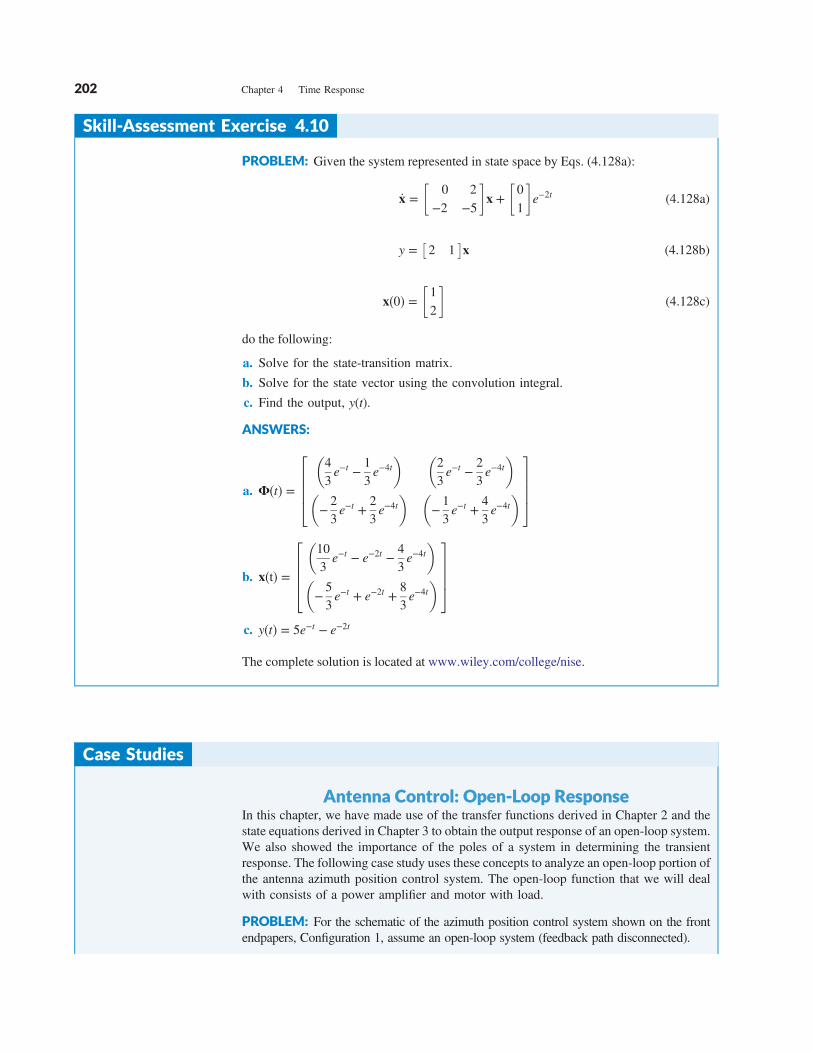
Skill-Assessment Exercise 4.10
PROBLEM: Given the system represented in state space by Eqs. (4.128a):
_x � 0 2
�2 �5
!
x � 0
1
!
e�2t (4.128a)
y � 2 1/ 0
x (4.128b)
x�0� � 1
2
!
(4.128c)
do the following:
a. Solve for the state-transition matrix.
b. Solve for the state vector using the convolution integral.
c. Find the output, y(t).
ANSWERS:
a. Φ�t� �
4
3e�t � 1
3e�4t
$ %
2
3e�t � 2
3e�4t
$ %
� 2
3e�t � 2
3e�4t
$ %
� 1
3e�t � 4
3e�4t
$ %
2
6
6
6
4
3
7
7
7
5
b. x�t� �
10
3e�t � e�2t � 4
3e�4t
$ %
� 5
3e�t � e�2t � 8
3e�4t
$ %
2
6
6
6
4
3
7
7
7
5
c. y�t� � 5e�t � e�2t
The complete solution is located at www.wiley.com/college/nise.
Case Studies
Antenna Control: Open-Loop ResponseAntenna Control: Open-Loop ResponseIn this chapter, we have made use of the transfer functions derived in Chapter 2 and the
state equations derived in Chapter 3 to obtain the output response of an open-loop system.
We also showed the importance of the poles of a system in determining the transient
response. The following case study uses these concepts to analyze an open-loop portion of
the antenna azimuth position control system. The open-loop function that we will deal
with consists of a power amplifier and motor with load.
PROBLEM: For the schematic of the azimuth position control system shown on the front
endpapers, Configuration 1, assume an open-loop system (feedback path disconnected).
202 Chapter 4 Time Response

a. Predict, by inspection, the form of the open-loop angular velocity response of the load
to a step-voltage input to the power amplifier.
b. Find the damping ratio and natural frequency of the open-loop system.
c. Derive the complete analytical expression for the open-loop angular velocity response
of the load to a step-voltage input to the power amplifier, using transfer functions.
d. Obtain the open-loop state and output equations.
e. Use MATLAB to obtain a plot of the open-loop angular velocityresponse to a step-voltage input.
SOLUTION: The transfer functions of the power amplifier, motor, and load as shown on
the front endpapers, Configuration 1, were discussed in the Chapter 2 case study. The two
subsystemsare shown interconnected inFigure 4.32(a).Differentiating the angular position
of themotor and loadoutputbymultiplyingby s,weobtain theoutput angularvelocity,ωo, as
shown in Figure 4.32(a). The equivalent transfer function representing the three
blocks in Figure 4.32(a) is the product of the individual transfer functions and is shown
in Figure 4.32(b).8
a. Using the transfer function shown in Figure 4.32(b), we can predict the nature of the
step response. The step response consists of the steady-state response generated by the
step input and the transient response, which is the sum of two exponentials generated
by each pole of the transfer function. Hence, the form of the response is
ωo�t� � A � Be�100t � Ce�1:71t �4.129�b. The damping ratio and natural frequency of the open-loop system can be found by
expanding the denominator of the transfer function. Since the open-loop transfer
function is
G�s� � 20:83
s2 � 101:71s � 171�4.130�
ωn �ffiffiffiffiffiffiffiffi
171p
� 13:08; and ζ � 3:89 (overdamped).
c. In order to derive the angular velocity response to a step input, we multiply the transfer
function of Eq. (4.130) by a step input, 1/s, and obtain
ωo�s� � 20:83
s�s � 100��s � 1:71� �4.131�
Motor and load
s
Power ampConvert to
angular velocity
Vp(s) 0.2083
s(s +1.71)
( )
( )
θ
a
b
Ea(s) o(s) ωo(s)100
(s +100)
20.83
(s +100)(s +1.71)
Vp(s) ωo(s)
FIGURE 4.32 Antenna azimuth position control system for angular velocity: a. forward path;
b. equivalent forward path
8This product relationship will be derived in Chapter 5.
Case Studies 203
Expanding into partial fractions, we get
ωo�s� � 0:122
s� 2:12 � 10�3
s � 100� 0:124
s � 1:71�4.132�
Transforming to the time domain yields
ωo�t� � 0:122 � �2:12 � 10�3�e�100t � 0:124e�1:71t �4.133�
d. First convert the transfer function into the state-space representation. Using
Eq. (4.130), we have
ωo�s�Vp�s�
� 20:83
s2 � 101:71s � 171�4.134�
Cross-multiplying and taking the inverse Laplace transform with zero initial
conditions, we have
_ωo � 101:71 _ωo � 171ωo � 20:83vp �4.135�
Defining the phase variables as
x1 � ωo (4.136a)
x2 � _ωo (4.136b)
and using Eq. (4.135), the state equations are written as
_x1 � x2 (4.137a)
_x2 � �171x1 � 101:71x2 � 20:83vp (4.137b)
where vp � 1, a unit step. Since x1 � ωo is the output, the output equation is
y � x1 �4.138�
Equations (4.137) and (4.138) can be programmed to obtain the step response
using MATLAB or alternative methods described in Appendix H.1 at www.wiley
.com/college/nise.
e. Students who are using MATLAB should now run ch4p4 in AppendixB. This exercise uses MATLAB to plot the step response.
CHALLENGE: You are now given a problem to test your knowledge of this chapter’s
objectives. Refer to the antenna azimuth position control system shown on the front
endpapers, Configuration 2. Assume an open-loop system (feedback path disconnected)
and do the following:
a. Predict the open-loop angular velocity response of the power amplifier, motor, and
load to a step voltage at the input to the power amplifier.
b. Find the damping ratio and natural frequency of the open-loop system.
204 Chapter 4 Time Response

c. Derive the open-loop angular velocity response of the power amplifier, motor, and load
to a step-voltage input using transfer functions.
d. Obtain the open-loop state and output equations.
e. Use MATLAB to obtain a plot of the open-loop angular velocityresponse to a step-voltage input.
Unmanned Free-Swimming SubmersibleVehicle: Open-Loop Pitch Response
Unmanned Free-Swimming SubmersibleVehicle: Open-Loop Pitch Response
An Unmanned Free-Swimming Submersible (UFSS) vehicle is shown in Figure 4.33. The
depth of the vehicle is controlled as follows. During forward motion, an elevator surface
on the vehicle is deflected by a selected amount. This deflection causes the vehicle to
rotate about the pitch axis. The pitch of the vehicle creates a vertical force that causes the
vehicle to submerge or rise. The pitch control system for the vehicle is used here and in
subsequent chapters as a case study to demonstrate the covered concepts. The block
diagram for the pitch control system is shown in Figure 4.34 and on the back endpapers for
future reference (Johnson, 1980). In this case study, we investigate the time response of
the vehicle dynamics that relate the pitch angle output to the elevator deflection input.
Cou
rtesy o
f th
e N
ava
l R
esearc
h L
abora
tory
.
FIGURE 4.33 Unmanned Free-Swimming Submersible (UFSS) vehicle
Pitch gain
–K1
Pitch
command
θc(s)
Commanded
elevator
de6ection
ec(s) 2
s +2
Elevator
actuator
Elevator
de6ection
e(s)
Vehicle
dynamics
–0.125(s +0.435)
(s +1.23)(s2+ 0.226s + 0.0169)
Pitch
θ(s)
Pitch rate
sensor
–K2s
+
–
+
–
δ δ
FIGURE 4.34 Pitch control loop for the UFSS vehicle
Case Studies 205

PROBLEM: The transfer function relating pitch angle, θ�s�, to elevator surface angle,
δe�s�, for the UFSS vehicle is
θ�s�δe�s�
� �0:125�s � 0:435��s � 1:23��s2 � 0:226s � 0:0169� �4.139�
a. Using only the second-order poles shown in the transfer function, predict percent
overshoot, rise time, peak time, and settling time.
b. Using Laplace transforms, find the analytical expression for the response of the pitch
angle to a step input in elevator surface deflection.
c. Evaluate the effect of the additional pole and zero on the validity of the second-order
approximation.
d. Plot the step response of the vehicle dynamics and verify your conclusions found in (c).
An animation PowerPoint presentation (PPT) demonstrating this system is available for
instructors at www.wiley.com/college/nise. See UFSS Vehicle.
SOLUTION:
a. Using thepolynomial s2 � 0:226s � 0:0169,wefind thatω2n � 0:0169 and2ζωn � 0:226.
Thus, ωn � 0:13 rad/s and ζ � 0:869. Hence, %OS � e�ζπ=ffiffiffiffiffiffiffiffi
1�ζ2p
100 � 0:399%.
From Figure 4.16, ωnT r � 2:75, or T r � 21:2 s. To find peak time, we use
Tp � π=ωn
ffiffiffiffiffiffiffiffiffiffiffiffi
1 � ζ2p
� 48:9 s. Finally, settling time is Ts � 4=ζωn � 35:4 s.
b. In order to display a positive final value in Part d. we find the response of the system to a
negative unit step, compensating for the negative sign in the transfer function. Using
partial-fraction expansion, the Laplace transform of the response, θ�s�, is
θ s� � � 0:125 s � 0:435� �s s � 1:23� � s2 � 0:226s � 0:0169� �
� 2:6161
s� 0:0645
1
s � 1:23
� 2:68 s � 0:113� � � 3:478ffiffiffiffiffiffiffiffiffiffiffiffiffiffiffiffi
0:00413p
s � 0:113� �2 � 0:00413�4.140�
Taking the inverse Laplace transform,
θ�t� � 2:616 � 0:0645e�1:23t
� e�0:113t�2:68 cos 0:0643t � 3:478 sin 0:0643t�
� 2:616 � 0:0645e�1:23t � 4:39e�0:113tcos�0:0643t � 52:38°� �4.141�
c. Looking at the relative amplitudes between the coefficient of the e�1:23t term and the
cosine term in Eq. (4.165), we see that there is pole-zero cancellation between
the pole at �1.23 and the zero at �0.435. Further, the pole at �1.23 is more than
five times farther from the jω axis than the second-order dominant poles at
�0:113� j 0:0643. We conclude that the response will be close to that predicted.
d. Plotting Eq. (4.141) or using a computer simulation, we obtain the step response shown
in Figure 4.35. We indeed see a response close to that predicted.
206 Chapter 4 Time Response

Students who are using MATLAB should now run ch4p5 in Appendix B.This exercise uses MATLAB to find ζ, ω, Ts, Tp, and Tr and plot a stepresponse. Table lookup is used to find Tr. The exercise applies theconcepts to the problem above.
CHALLENGE: You are now given a problem to test your
knowledge of this chapter’s objectives. This problem uses
the same principles that were applied to the Unmanned
Free-Swimming Submersible vehicle: Ships at sea undergo
motion about their roll axis, as shown in Figure 4.36. Fins
called stabilizers are used to reduce this rolling motion. The
stabilizers can be positioned by a closed-loop roll control
system that consists of components, such as fin actuators
and sensors, as well as the ship’s roll dynamics.
Assume the roll dynamics, which relates the roll-angle
output, θ�s�, to a disturbance-torque input, TD(s), is
θ�s�TD�s� � 2:25
�s2 � 0:5s � 2:25� �4.142�
Do the following:
a. Find the natural frequency, damping ratio, peak time, settling time, rise time, and percent
overshoot.
b. Find the analytical expression for the output response to a unit step input in voltage.
c. Use MATLAB to solve a and b and to plot the response found in b.
5 10 15 20 25 30 35 40 45 500
0.5
1.0
1.5
2.0
2.5
3.0
Negative pitch angle response (radians)
Time (seconds)
FIGURE 4.35 Negative step response of pitch control for UFSS vehicle
θTD(t)
Roll axis
(t)
FIGURE 4.36 A ship at sea, showing roll axis
Case Studies 207

Summary
In this chapter, we took the system models developed in Chapters 2 and 3 and found the
output response for a given input, usually a step. The step response yields a clear picture of
the system’s transient response. We performed this analysis for two types of systems, first
order and second order, which are representative of many physical systems. We then
formalized our findings and arrived at numerical specifications describing the responses.
For first-order systems having a single pole on the real axis, the specification of
transient response that we derived was the time constant, which is the reciprocal of the
real-axis pole location. This specification gives us an indication of the speed of the transient
response. In particular, the time constant is the time for the step response to reach 63% of its
final value.
Second-order systems are more complex. Depending on the values of system
components, a second-order system can exhibit four kinds of behavior:
1. Overdamped
2. Underdamped
3. Undamped
4. Critically damped
We found that the poles of the input generate the forced response, whereas the system
poles generate the transient response. If the system poles are real, the system exhibits
overdamped behavior. These exponential responses have time constants equal to the reciprocals
of the pole locations. Purely imaginary poles yield undamped sinusoidal oscillations whose
radian frequency is equal to the magnitude of the imaginary pole. Systems with complex poles
display underdamped responses. The real part of the complex pole dictates the exponential
decayenvelope, and the imaginarypart dictates the sinusoidal radian frequency.Theexponential
decay envelope has a time constant equal to the reciprocal of the real part of the pole, and the
sinusoid has a radian frequency equal to the imaginary part of the pole.
For all second-order cases, we developed specifications called the damping ratio, ζ,
and natural frequency, ωn. The damping ratio gives us an idea about the nature of the
transient response and how much overshoot and oscillation it undergoes, regardless of time
scaling. The natural frequency gives an indication of the speed of the response.
We found that the value of ζ determines the form of the second-order natural response:
� If ζ � 0, the response is undamped.
� If ζ < 1, the response is underdamped.
� If ζ � 1, the response is critically damped.
� If ζ > 1, the response is overdamped.
The natural frequency is the frequency of oscillation if all damping is removed. It acts
as a scaling factor for the response, as can be seen from Eq. (4.28), in which the independent
variable can be considered to be ωnt.
For the underdamped case we defined several transient response specifications,
including these:
� Percent overshoot, %OS
� Peak time, Tp
� Settling time, T s
� Rise time, T r
208 Chapter 4 Time Response

The peak time is inversely proportional to the imaginary part of the complex pole. Thus,
horizontal lines on the s-plane are lines of constant peak time. Percent overshoot is a
function of only the damping ratio. Consequently, radial lines are lines of constant percent
overshoot. Finally, settling time is inversely proportional to the real part of the complex
pole. Hence, vertical lines on the s-plane are lines of constant settling time.
We found that peak time, percent overshoot, and settling time are related to pole location.
Thus,we can design transient responses by relating a desired response to a pole locationand then
relating that pole location to a transfer function and the system’s components.
The effects of nonlinearities, such as saturation, dead zone, and backlash, were
explored using MATLAB’s Simulink.
In this chapter, we also evaluated the time response using the state-space approach.
The response found in this way was separated into the zero-input response, and the
zero-state response, whereas the frequency response method yielded a total response
divided into natural response and forced response components.
In the next chapter we will use the transient response specifications developed here
to analyze and design systems that consist of the interconnection of multiple subsystems.
We will see how to reduce these systems to a single transfer function in order to apply the
concepts developed in Chapter 4.
Review Questions
1. Name the performance specification for first-order systems.
2. What does the performance specification for a first-order system tell us?
3. In a system with an input and an output, what poles generate the steady-state response?
4. In a system with an input and an output, what poles generate the transient response?
5. The imaginary part of a pole generates what part of a response?
6. The real part of a pole generates what part of a response?
7. What is the difference between the natural frequency and the damped frequency of
oscillation?
8. If a pole is moved with a constant imaginary part, what will the responses have in
common?
9. If a pole is moved with a constant real part, what will the responses have in common?
10. If a pole is moved along a radial line extending from the origin, what will the responses
have in common?
11. List five specifications for a second-order underdamped system.
12. For Question 11 how many specifications completely determine the response?
13. What pole locations characterize (1) the underdamped system, (2) the overdamped
system, and (3) the critically damped system?
14. Name two conditions under which the response generated by a pole can be neglected.
15. How can you justify pole-zero cancellation?
16. Does the solution of the state equation yield the output response of the system? Explain.
17. What is the relationship between �sI � A�, which appeared during the Laplace transfor-
mation solution of the state equations, and the state-transition matrix, which appeared
during the classical solution of the state equation?
18. Name a major advantage of using time-domain techniques for the solution of the
response.
19. Name a major advantage of using frequency-domain techniques for the solution of the
response.
Review Questions 209
Related Documents