Time-Optimal Interpolation of CNC Machines along ...xgao/papernc/29-09.pdf · Time-Optimal Interpolation of CNC Machines ... @mmrc.iss.ac.cn. ... optimal velocity planning method

Mathematics Mechanization Research PreprintsKLMM, Chinese Academy of SciencesVol. 29, 165–188, September 2010 165

Time-Optimal Interpolation of CNC Machines

along Parametric Path with Chord Error and

Tangential Acceleration Bounds

Chun-Ming Yuan, Xiao-Shan GaoKLMM, Institute of Systems Science, Chinese Academy of Sciences

E-mail: (cmyuan,xgao)@mmrc.iss.ac.cn.

Abstract. Interpolation and velocity planning for parametric curves are crucial prob-lems in CNC machining. In this paper, a time-optimal velocity planning algorithm undera given chord error bound and a tangential acceleration bound is proposed. The key ideais to reduce the chord error bound to a centripetal acceleration bound which leads toa velocity limit curve, called the chord error velocity limit curve (CEVLC). Then, thevelocity planning is to find the time-optimal velocity curve governed by the tangentialacceleration bound “under” the CEVLC. For two types of simple splines, explicit for-mulas for the optimal velocity curve are given. We implement the methods in these twocases and use curved segments from real machining parts to show the feasibility of themethods.

Keywords. Parametric curve interpolation, time-optimal velocity planning, chord error,velocity limit curve.

1 introduction

In modern CAD systems, the standard representation for free form surfaces is parametricfunctions. While the conventional computed numerically controlled (CNC) systems mainlyuse micro line segments (G01 codes) to represent the machining path. To convert the para-metric curves into line segments is not only time consuming but also leads to problems suchas large data storage, speed fluctuation, and poor machining accuracy. In the seminal work[5, 18, 22], Chou, Yang, and Shpitalni et al proposed to use parametric curves generated inCAD/CAM systems directly in the CNC systems to overcome these drawbacks.

An interpolation algorithm usually consists of two phases: velocity planning and parame-ter computation. Let C(u) be the manufacturing path. The phase to determine the feed-ratev(u) along C(u) is called velocity planning. When the feed-rate v(u) is known, the way tocompute the next interpolation point at ui+1 = ui +4u during one sampling time period iscalled parameter computation.

This paper focuses on velocity planning along a spatial parametric path. For the param-eter computation phase, please refer to [4, 9, 21] and the literatures in them. Two types ofacceleration modes can be used in the velocity planning: the tangential acceleration and themulti-axis acceleration where each axis accelerates independently.

Due to its conceptual simplicity, the tangential acceleration is widely used in CNC in-terpolations. Bedi et al[1] and Yang-Kong[22] used a uniform parametric feed-rate without

166 C.M. Yuan and X.S. Gao

considering the chord error. Yeh and Hsu used a chord error bound to control the feed-rate ifneeded and used a constant feedarte in other places [23]. However, the machine accelerationcapabilities were not considered. Narayanaswami and Yong [24] gave a velocity planningmethod based on tangential acceleration bounds by computing maximal passing velocitiesat sensitive corners. Cheng and Tsai [4] gave an interpolation method based on differentvelocity profiles for tangential ACC/DCC feed-rate planning. Velocity planning methodswith tangential acceleration and jerk bounds were considered by several research groups[7, 11, 13, 14, 12]. In particular, Emami and Arezoo [6], Lai et al[10] proposed velocityplanning methods with confined acceleration, jerk, and chord error constraints by checkingthese values at every sampling point and using backtracking to adjust the velocity if anyof the bounds is violated. In all the above methods besides [6, 10, 23], the chord error isconsidered only at some special points, and there is no guarantee that the chord error issatisfied at all points. Furthermore, all these methods are not proved to be time-optimal.

In the multi-axis acceleration case, Borow [3] and Shiller et al [16, 15] presented a time-optimal velocity planning method for a robot moving along a curved path with accelerationbounds for each axis. Farouki and Timar [19, 20] proposed a time-optimal velocity planningalgorithm in CNC machining under the same acceleration constraints. Following the methodin [19, 20], Zhang et at gave a simplified time-optimal velocity planning method for quadraticB-splines and realized real-time manufacturing on industrial CNC machines [26]. Zhang etal[25] gave a greedy algorithm for velocity planning under multi-axis jerk constraints. Theseoptimal methods use the “Bang-Bang” control strategy, that is, at least one of the axesreaches its acceleration bound all the time. But they do not consider the chord error whichis an important factor for CNC-machining.

In this paper, we give a time-optimal velocity planning algorithm along a parametriccurve path C(u) under a given chord error bound and a tangential acceleration bound. Themain contribution of the paper is the introduction of the chord error velocity limit curve(abbr. CEVLC) and the velocity planning algorithm.

We show that the chord error bound can be approximately reduced to a centripetalacceleration bound. Furthermore, if the centripetal acceleration reaches its maximal bound,the velocity can be written as an algebraic function in the parameter u of the curve pathC(u). The graph of this function is called the CEVLC. The CEVLC is significant because thefinal velocity curve must be “under” this curve or be part of this curve, which narrows therange of velocity planning. Also, certain key points on the CEVLC, such as the discontinuouspoints, play an important role in the velocity planning.

Similar to the previous work on time-optimal velocity planning, our algorithm also usesthe “Bang-Bang” control strategy, which is a necessary condition for time optimal in ourcase. Then the final velocity curve is governed either by the centripetal acceleration boundor by the tangential acceleration bound, and the later one is called the integration velocitycurve. The main task of the velocity planning is to find the switching points between theintegration velocity curve and the CELVC.

Two main results on the optimal velocity curve are given in this paper. Firstly, as atheoretical result, we show that the final velocity is the minimum of the CEVLC and allthe integration velocity curves passing through the initial point, the termination point, andthe key points of the CEVLC. We also give a practical algorithm to compute the optimal

Time-Optimal Control of CNC Machines with Chord Error 167

velocity curve incrementally. For quadratic splines and cubic PH curves, the integrationvelocity curve can be given by explicit formulas. We implement our algorithm in these twocases and conduct experiments using curved pathes from real manufacturing parts.

Moreover, we also give a simple and real-time feed-rate override algorithm based on ourvelocity planning curve. For multi-axis velocity planning algorithms, feed-rate override iscomplicated and not suitable for real time interpolation.

As a final remark, we want to mention that by combining the CEVLC proposed in thispaper and the method proposed in [19, 20], it is possible to give a time optimal velocityplanning method under a given chord error bound and multi-axis acceleration bounds.

The rest of the paper will be organized as follows. Section 2 gives the time-optimalvelocity planning algorithm for a parametric curve. Section 3 gives the details for computingthe time optimal velocity curves for quadratic B-spline and cubic PH-spline. Section 4 givesa feed-rate override algorithm for CNC-machining. Section 5 concludes the paper.

2 Time-optimal velocity planning under chord error and tan-gential acceleration bound

The time-optimal velocity planning algorithm will be presented in this section. We consider aspatial piecewise parametric curve C(u), u = 0..1 with C1 continuity, such as splines, Nurbs,etc. We further assume that each piece of the curve is differentiable to the third order andhas left and right limitations at the endpoints.

2.1 Problem

In order to control the machine tools, we need to know the velocity of the movement at eachpoint on the curve, which is denoted as a function v(u) in the parameter u and is called thevelocity curve. The procedure to compute the velocity curve v(u) is called velocity planning.In this subsection, we will show that the chord error bound can be reduced to the centripetalacceleration bound and formulate the velocity planning problem as an optimization problemwith tangential and centripetal acceleration bounds.

For a parametric curve C(u), we denote its parametric speed to be:

σ(u) =ds

du= |C ′(u)|,

where ′ is the derivative w.r.t. u. The curvature and radius of curvature are defined to be:

k(u) =|C ′(u)× C ′′(u)|

σ(u)3, ρ(u) =

1k(u)

.

|PQ|: chord error

P

Q

Fig. 1. The chord error


The cutter moves in a line segment between two adjacent points on the curve C(u) andthe distance between the line segment and the curve segment is called the chord error whichis the main source of the manufacturing error (Fig 1). Firstly, we will show that the chorderror bound can be reduced to the centripetal acceleration bound.

Let T be the sampling period, δ the error constraint, and ±A the tangential accelerationbounds. In practice, the chord error bound is much less than the radius of curvature at eachpoint on the curve. By the chord error formula [23], at each parametric value u,

q(u) = v2(u) ≤ 8δρ(u)− 4δ2

T 2≈

8δρ(u)T 2

=8δ

k(u)T 2.

If we denote by d(u) the interpolating chord error at u with feed-rate v(u), then d(u) =T 2v(u)2

8ρ(u) ≤ δ. LetaN (u) = v(u)2/ρ(u) = k(u)v(u)2 = k(u)q(u) (1)

be the centripetal acceleration and

B =8δ

T 2. (2)

Then, the chord error bound is transformed to the centripetal acceleration bound:

d(u) ≤ δ ⇐⇒ aN (u) ≤ B.

Sinced

dt=

ds

dt

du

ds

d

du=

v

σ

d

du, (3)

The tangential acceleration is:

aT (u) =dv(u)

dt=

v(u)v′(u)σ(u)

=q′(u)2σ(u)

. (4)

From (3), the time optimal velocity planning problem becomes the following optimizationproblem: to find a velocity curve v(u) such that

minv(u)

t =∫ 1

0

σ(u)v(u)

du, (5)

with the tangential and centripetal acceleration constraints

|aT (u)| ≤ A, aN (u) ≤ B, u = 0..1, (6)

where (aT (u), aN (u)) are the tangential and centripetal accelerations and (A,B) are theirbounds respectively. Note that B can be derived from the chord error bound from (2).


2.2 The main result

In this section, we present the main result of the paper about the time optimal velocityplanning problem (5). We will give a velocity planning algorithm in section 2.4 and provethe correctness of the result in section 2.5.

Before giving the main result, we need to introduce several basic concepts. We use“Bang-Bang” control, that is, at least one of “=” holds among the inequalities in (6). Thiswill lead to two cases.

If the centripetal acceleration reaches its bound B, then from (1) we have q(u) = Bk(u) ,

which defines a curve

qlim(u) = v2lim(u) = B/k(u), u ∈ [0, 1] or (7)

vlim(u) =√

B/k(u), u ∈ [0, 1],

in the u-v plane with v as the vertical axis. We call this curve the velocity limit curve with thechord error constraint, denoted by CEVLC. If C(u) is a piecewise curve with C1 continuity,then its CEVLC is the combination of the CEVLCs of its components. From the constraintaN ≤ B, the velocity curve must be “under” the CEVLC in the v direction.

Example 2.1 If C(u) = ( 2u1+u2 , 1−u2

1+u2 , 0) and B = 100, then vlim(u) = 10, u ∈ [0, 1].

If C(u) = (u2+u+1, u2+2u−1, 2u+1) and B = 600, then vlim(u) = 10(8u2+12u+9)34 , u ∈

[0, 1].If C(u) = (1

3u3 − 4u2 − 8u, 23u3 + 3u2 − 8u,−2

3u3 − 2u2 − 14u) and B = 1000, thenvlim(u) = 30u2 + 40u + 180, u ∈ [0, 1].

If the tangential acceleration reaches its bound, then from (4) the square of the velocityq(u) = v(u)2 can be obtained by solving the differential equation q′(u) = ±2Aσ(u), whosesolution is

q = ±2Aπ(u) + c, (8)

where π(u) =∫

σdu is the primitive function of σ(u) and c a constant which can be deter-mined by an initial point (u∗, q(u∗)):

c = q(u∗)∓ 2Aπ(u∗).

The curve (8) is called the integration curve or the integration trajectory.Let vP (u) be the integration trajectory with tangential acceleration A starting from an

initial point P = (uP , vlim(uP )) both for the forward (the +u) and the backward (the−u) directions. Let v0(u) be the forward integration trajectory with tangential accelerationA from the initial point P0 = (0, 0) and v1(u) the backward integration trajectory withtangential acceleration A from the initial point P1 = (1, 0). Of curse, all the curves mentionedabove are defined in [0, 1].

Then, the solution to the optimization problem (5) is given below.

Theorem 2.2 Let K be the finite set of key points of the CEVLC to be defined in the nextsection. Then

v(u) = minP∈K

(vlim(u), vP (u), v0(u), v1(u)). (9)

Then, v(u) is the solution to the optimal problem (5).


Obviously, v(u) is a piecewise continuous curve for u ∈ [0, 1]. We will prove the theorem inSection 2.5.

2.3 Key points of the CEVLC

There exist three types of special points on the CEVLC, which are called switching pointsor key points.

The first type switching points are the discontinuous points of the CEVLC. These pointscorrespond to the curvature discontinuous points of the original curve. They must be thesingular points of the parametric curve or the connection points of two curve segments. Ifwe denote by C(u) the curve segment, then the singular points of C(u) can be computedby solving the equations C ′(u)× C ′′(u) = 0. From (7), the limit velocity vlim is ∞ at thesepoints and the real velocity curve can not reach it, so we can omit the singular points fromthe key points. Thus, only the connection points need to be considered.

At a first type key point, the velocity is not continuous and we call the smaller one ofthe left and right side velocities as the minimal velocity or simply the velocity of this point.

The second type switching points are the continuous but non-differentiable points of theCEVLC (slope discontinuity). These points correspond to the curvature continuous but non-differentiable points of the original curve. Hence, they must be the connection points of twocurve segments.

For a differentiable segment of the CEVLC divided by the above two types of key points,we can divide it according to whether the tangential acceleration of the CEVLC is ±A, whereA is from (6). A point on the CEVLC is called a key point of the third type if the tangentialacceleration along the CEVLC at this point is ±A. We can find the third type key pointsby solving the following algebraic equation in u

aT (u) =qlim(u)2σ(u)

=Bσ(u)2

2|C ′(u)× C ′′(u)| = ±A.

With these switching points, the CEVLC is divided into two types of segments:

1. A curve segment is called feasible if the absolution values of tangential acceleration atall points are bounded by A. A feasible CEVLC segment can be a part of the finalvelocity curve.

2. A curve segment is called unfeasible if the absolution values of tangential accelerationat all points are larger than A. An unfeasible CEVLC segment cannot be a part of thefinal velocity curve. In other words, the final velocity curve must be strictly under it.

If the curve segments on the left and right sides of a second type key point are bothfeasible, we delete this key point.

2.4 The time optimal velocity planning algorithm

We use the “Bang-Bang” control strategy. Then the real velocity curve is governed eitherby the maximal centripetal acceleration or by the maximal tangential acceleration. Sincethe velocity curve must be under or be a part of the CEVLC, we need to find the proper


integration trajectory under the CEVLC. We first give the main idea of the velocity planningalgorithm.

Firstly, we compute the CEVLC, find the key points and their speeds. Compute theforward integration trajectory vs from the starting point (0, 0) with tangential accelerationA. Find the intersection point (ul, vs(ul)) of vs and the CEVLC. Compute the backwardintegration trajectory ve from the ending point (1, 0) with tangential acceleration A. Findthe intersection point (ur, ve(ur)) of ve and the CEVLC.

Secondly, if (ul, vs(ul)) = (ur, ve(ur)), then return the combination of vs and ve as thefinal velocity curve. If ul > ur, find the intersection point of vs and ve and return thecombination of vs and ve as the final velocity curve. Otherwise, set Pc = (ul, vs(ul)) to bethe current point and consider the following three cases.

If the next segment of CEVLC from point Pc in the forward direction (the +u direction)is feasible, then we merge this feasible segment into vs and set the current point (ul, vs(ul))to be the end point of this segment.

If the next segment of CEVLC from point Pc in the forward direction is not feasible andthe forward integration trajectory vf with initial point Pc is under the CEVLC, then let(ui, vf (ui)) be the intersection point of vf and the CEVLC. Merge vf (u), u ∈ [ur, ui] into vs.Let ul = ui and Pc = (ul, vf (ul)).

If the next segment of CEVLC from point Pc in the forward direction is not feasible andthe integration trajectory vf with initial point Pc is above the CEVLC, then we find thenext key point Pn on the right hand side of Pc. From Pn, compute the backward integrationtrajectory vb, find the intersection point of vb with vs, and merge vb and vs as the new vs.Set Pn as the new current point.

Finally, with the new current point, we can repeat the procedure from the second stepuntil the velocity curve is found.

Here by saying a forward curve v1(u) is under or above another curve v2(u) from a pointP = v1(u∗), we mean that v1(u) is under or above v2(u) in a neighborhood of u∗ in theforward direction.

To describe our algorithm precisely, we need the following notations. For a discontinuouscurve f1(x), we denote by f+

1 (x∗) and f−1 (x∗) the limitations of f1(x) at x∗ from the leftand right hand sides respectively, and define f1(x∗) = min(f+

1 (x∗), f−1 (x∗)). Let f2(x) bea curve with C0 continuity. If f2(x∗) = f1(x∗) or f2(x∗) is between the left and rightlimitations of f1(x) at x∗, then define (x∗, f2(x∗)) to be the intersect point of the curves(x, f2(x)) and (x, f1(x)).

We now give the velocity planning algorithm.

Algorithm VP CETA. The input of the algorithm is the curve C(u), u ∈ [0, 1], a chorderror bound d, and a tangential acceleration bound A. The output is the velocity curvevc(u), u ∈ [0, 1] which is the solution to the optimization problem (5).

1 Compute the CEVLC in (7) and its key points as shown in section 2.3. Denote by Uf theparametric intervals where the corresponding segments of the CEVLC are feasible.

2 From the starting point (0, 0), compute the forward integration trajectory vs using thetangential acceleration A. Compute the first intersection point (ul, vs(ul)) of vs andthe CEVLC. If there exists no intersection, denote ul = 1.


3 From the ending point (1, 0), compute the backward integration trajectory ve using thetangential acceleration A. Compute the first intersection point (ur, ve(ur)) of ve andthe CEVLC. If there exists no intersection, denote ur = 0.

4 If (ul, vs(ul)) = (ur, ve(ur)), then return the combination of vs and ve as the final velocitycurve. If ul > ur, find the intersection point (ui, vs(ui)) of vs and ve, return v(u),where

v(u) =

{vs, 0 ≤ u ≤ ui

ve, ui < u ≤ 1.(10)

5 If (ul, vlim(ul)) is a discontinuous point on the CEVLC, there are three possibilities.

(a1) If v+lim(ul) > vs(ul) = v−lim(ul), goto step 6.

(a2) If v+lim(ul) = vs(ul) < v−lim(ul), goto step 8.

(a3) If v+lim(ul) ≥ vs(ul) > v−lim(ul), let un = ul and goto step 9.

6 Now, (ul, vs(ul)) is the starting point of the next segment of CEVLC. There exist threecases.

(b1) If the next segment of the CEVLC is feasible, goto step 7

(b2) If a−T (ul) ≥ A, goto step 8.

(b3) If a−T (ul) ≤ −A, then find the next key point (un, vlim(un)) along the +u directionand goto step 9.

7 Let un > ul be the parameter of the next key point. Then, (ul, un) ⊂ Uf . Update vs tobe

vs(u) =

{vs(u), 0 ≤ u < ul

vlim(u), ul ≤ u ≤ un.

Let ul = un, goto step 4.

u=ulvlim

vlim

vf

(a) Case (a2)

vlim

vlim

vf

u=ul

(b) Case (b2)

Fig. 2. Two cases of step 8: computation of forward integration curve

8 Starting from (ul, vs(ul)), compute the forward integration trajectory vf with tangentialacceleration A. Find the first intersection point (ui, vf (ui)) of vf and the CEVLC (Fig.2). If there exists no intersection, denote ul = 1. Update vs to be

vs(u) =

{vs(u), 0 ≤ u < ul

vf (u), ul ≤ u ≤ ui.


u=un

vlim

vs

vb

vlim

(a) Case (a3)

vb

u=un

vlim

vs

(b) Case (b3)

Fig. 3. Two cases of step 9: computation of backward integration curve

Let ul = ui, goto step 4.

9 Starting from point (un, vlim(un)), compute the backward integration trajectory vb in the−u direction with tangential acceleration A. Find the intersection point1) (ui, vb(ui))of vb and vs. See Fig. 3 for an illustration. Update vs to be

vs(u) =

{vs(u), 0 ≤ u < ui

vb(u), ui ≤ u ≤ un.

Let ul = un, goto step 4.

The correctness proof of the algorithm is given in Section 2.5. Further improvements ofthe algorithm are given in Section 2.6.

The flow chart of the above algorithm is given in Fig. 5. The details of the algorithm isomitted in the figure.

40

50

60

70

80

90

100

110

0 0.2 0.4 0.6 0.8 1

x

(a) CEVLC and key points

0

20

40

60

80

100

0.2 0.4 0.6 0.8 1

I

II

III

IV

V

VI

VII

(b) velocity curve

Fig. 4. An illustrative example of velocity planning

Figure 4 is an illustrative example of the algorithm.Compute the CEVLC vlim and the key points as shown in Figure 4(a), where ◦ represents

the key points of first type and the corresponding parameters are 0.2, 0.7; ¦ represents thekey point of second type, and the corresponding parameter is 0.4; and ¤ represents the keypoints of third type. The gray parts are feasible segments.

1)We will show that there exists a unique intersection point.


Starting from point (u, v) = (0, 0), compute the forward integration trajectory vs whichintersects the CEVLC at u = 0.2. Starting from (u, v) = (1, 0), compute the backwardintegration trajectory ve which intersects the CEVLC at u = 0.7.

In step 5, the current point Pc is a discontinues point and case (a3) is executed. Instep 9, starting from the first ◦ point, compute the backward integration trajectory vb whichintersects vs at the first point marked by +. Update vs to be the piecewise curve marked byI, II in Figure 4(b).

From the first point marked by ◦, the CEVLC is feasible. Hence, update vs to be thepiecewise curve marked by I, II and the first gray part of the CEVLC(III).

Let the key point marked by ¦ be the current point. From the current point, the CEVLCis not feasible and case (b3) is executed. In step 9, we select the next key point which isthe first point marked by ¤. Starting from this point, compute the backward integrationtrajectory vb which intersects vs at the second point marked by +. Update vs to be thepiecewise curve marked by I, II, III, IV in the figure.

Starting from the first point marked by ¤, the CEVLC is feasible. Hence, update vs tobe the piecewise curve marked by I, II, III, IV,V in the figure.

Let the second point marked by ¤ to be the current point. Starting from this point, theCEVLC is not feasible and case (b2) is executed. In step 8, compute the forward integrationtrajectory vf which intersects ve at the third point marked by +. The final velocity curveconsists of seven pieces marked by I, II, III, IV,V,VI, and VII in the figure.

Note that the CEVLC can be parts of the final velocity curve quite often, while in [19, 20],the VLC is rarely a part of the final velocity curve.

Remark 2.3 In the above algorithm, we need to compute the CEVLC and its key points, theintegration trajectory, the intersection points of the integration trajectory and the CEVLC,and the intersection points of two integration trajectories. In principle, these computationscan be reduced to computing integrations and solving algebraic equations. In Section 3, wewill show how to give explicit formulas for the integration curve for two types of special typesof curves.

2.5 The correctness of the algorithm

In this section, we will show that the velocity curve given by the algorithm in the precedingsubsection is the only solution to the optimization problem (5). The proof is divided intotwo parts. We will first show that the velocity curve computed by the algorithm is the curvedefined in (9) and then prove that this velocity curve is the solution to the problem (5). Inorder to prove this, we need the following result.

Theorem 2.4 [2][p.24-26] Let y, z be solutions of the following differential equations

y′ = F (x, y), z′ = G(x, z),

respectively, where F (x, y) ≤ G(x, y), a ≤ x ≤ b, and F or G satisfies Lipschitz’s condition.If y(a) = z(a), then y(x) ≤ z(x) for any x ∈ [a, b].

In our case, the above theorem implies the following result.


Fig. 5. Flow chart of the velocity planning


Lemma 2.5 Let v1(u) and v2(u) be two velocity curves for the curve C(u) and [u1, u2] ⊂[0, 1]. If v1(u1) ≤ v2(u1) and aT1(u) ≤ aT2(u) for u ∈ [u1, u2], then v1(u) ≤ v2(u) foru ∈ [u1, u2]. Furthermore, if v1(u1) < v2(u1), then v1(u) < v2(u) for u ∈ [u1, u2].

Proof. We may assume that v1(u1) = v2(u2), since if v1(u1) < v2(u1), we may considerv̄2(u) = v2(u)− v2(u1) + v1(u1) which still satisfies the conditions in the lemma. Since C(u)is differentiable to the order of three, σ(u) and aT1(u) must be bounded in [u1, u2]. From(4), q′1(u) = 2σ(u)aT2(u) and q′2(u) = 2σ(u)aT2(u). Then, we have q1(u1) = v1(u1)2 =q2(u1) = v2(u1)2, 2σ(u)aT2(u) ≤ 2σ(u)aT2(u) for u ∈ [u1, u2], and 2σ(u)aT1(u) satisfies theLipschitz’s condition. Using Theorem 2.4, we have v1(u) ≤ v2(u) for u ∈ [u1, u2]. The secondpart of the lemma can be proved similarly.

Before giving the correctness proof, we first explain the key steps of the algorithm.Besides the in initial steps, new velocity trajectories are generated in Steps 7, 8, 9. Wewill show that these steps are correct in the sense that they will really generate new velocitytrajectories. Step 7 is obvious, since we will use the next feasible CEVLC segment as thevelocity trajectory. Two cases lead to step 8: cases (a2) and (b2). In case (a2), we havev+lim(ul) = vs(ul) < v−lim(ul), which means there exists a parameter un > ul such that

vlim(u) > vs(ul) for u ∈ (ul, un). As a consequence, starting at (ul, vs(ul)), we can usethe tangential acceleration A to generate a piece of integration trajectory without violatethe CEVLC (See Fig. 2(a)). In case (b2), there exists a parameter un > ul such that thetangential acceleration of the CEVLC must be strictly larger than A for u ∈ (ul, un). ByLemma 2.5, starting from point (ul, vs(ul)), we can use the tangential acceleration A withoutviolate the CEVLC (See Fig. 2(b)). We thus prove the correctness of step 8. The correctnessstep 9 can be proved in a similar way. Furthermore, we have

Lemma 2.6 In step 9 of the algorithm, the backward integration trajectory vb intersects vs

only once if there exist no overlap curve segments.

Proof. Two situations lead to the execution of step 9: step (a3) and step (b3). In case(a3), the key point at ul is of the first type and v+

lim(ul) ≥ vs(ul) > v−lim(ul). Then vs

and vb must intersect because vb decreasing with the acceleration −A and vs is boundedby ±A. By Lemma 2.5, vs and vc can intersects only once if there exist no overlap curvesegments. Moreover, if there exists an overlap curve segment of vb and vs, then there existsno intersection point of vb and vs except the overlap curve segment by Lemma 2.5. Case(b3) can be proved similarly.

Similarly, we can show that vs and ve in step 4 of the algorithm only intersect once ifthere exist no overlap curve segments. And we can use the bisection method to compute theintersection point.

We now prove the main result of the paper.

Theorem 2.7 The velocity curve computed with Algorithm VP CTEA is the velocity curvedefined in equation (9) and is the only solution to the optimization problem (5).

Proof. Let v(u) be the velocity curve computed with the algorithm. It is clear that v(u)is below the CEVLC and the tangential acceleration aT (u) of v(u) satisfies |aT (u)| ≤ A.


Also, if |aT (u)| 6= A, the corresponding v(u) must be a segment of feasible CEVLC. As aconsequence, v(u) satisfies conditions (6) and is bang-bang.

From the algorithm, it is clear that v(u) consists of pieces of vP (u) for all key points Pof the CEVLC including the start point (0, 0) and the ending point (1, 0). To prove (9), itsuffices to show that for each key point P , if vP (u∗) 6= v(u∗) for a parametric value u∗, thenvP (u∗) > v(u∗). From the algorithm, it is clear that all key points including the startingand ending points are on or above v(u). Let P = (u0, v0) be a key point. Then v0 ≥ v(u0).In [u0, 1], the tangential acceleration of vP (u) is A. Then by lemma 2.5, vP (u) ≥ v(u) foru ∈ [u0, 1]. In [0, u0], if we consider the movement from u0 to 0, then the acceleration ofvP (u) is also A, and hence vP (u) ≥ v(u) for u ∈ [0, u0]. As a consequence, vP (u) cannot bestrictly under v(u) at any u. We thus prove that v(s) is the curve in (9).

We now prove that v(s) is an optimal solution. We will prove a stronger result, that is,the velocity curve q(u) = v2(u) obtained by the algorithm is the maximally possible velocityat each parametric value u. To prove this, we assume that there exists another velocitycurve v∗(u) satisfying the constraints listed in (6), and there exists a u∗ ∈ [0, 1] such thatv∗(u∗) > v(u∗). Let q∗(u) = v2∗(u).

The parametric interval [0, 1] is divided into sub-intervals by the key points of CEVLCon the final velocity curve and intersection points in steps 4, 8, 9 of the algorithm. From thealgorithm, we can see that on each of these intervals, v(u) could be a segment of the CEVLC,an integration trajectory with tangential acceleration A in the +u direction, which is calledan increasing interval, or an integration trajectory with tangential acceleration −A in the+u direction, which is called a decreasing interval. Furthermore, if [u1, u2] is an increasinginterval, the starting point (u1, v(u1)) must be a key point of the CEVLC; if [u1, u2] is adecreasing interval, the end point (u2, v(u2)) must be a key point of the CEVLC.

According to the definition of the CEVLC, u∗ cannot be on the CEVLC and thus mustbe in an increasing or decreasing interval. Firstly, let u∗ be in an increasing interval [u1, u2].Since (u1, v(u1)) is a key point on the CEVLC, we have v∗(u1) ≤ v(u1). Since v∗(u∗) > v(u∗)and v∗, v are continuous curves, there exists a u0 ∈ [u1, u∗] such that v∗(u0) = v(u0). On[u0, u∗], using Lemma 2.5, we obtain a contradiction. Secondly, let u∗ ∈ [u1, u2] and [u1, u2]be a decreasing interval. We can consider the movement from u2 to u1 and the accelerationof v becomes A and the theorem can be proved similarly to the case of increasing intervals.

2.6 Further improvements of the algorithm

In this section, we present modifications to Algorithm VP CETA to improve its efficiencyby getting rid of some unnecessary computations.

We first prove a lemma.

Lemma 2.8 Let (ul, vlim(ul)) and (un, vlim(un)) be two adjacent key points of the CEVLC.Then an integration trajectory intersects the curve segment vlim(u), u ∈ (ul, un) once at most.

Proof. We denote by i(u) an integration trajectory. Without loss of generality, we assumethat the tangential acceleration of i(u) is A; otherwise, consider the −u direction. Since thetwo key points are adjacent, there are three cases: (a): aT (u) > A, (b): aT (u) < −A, or (c):


−A < aT (u) < A2) for u ∈ (ul, un).Case (a). Since i(ul) ≤ vlim(ul), we have i(u) < vlim(u) for u ∈ (ul, un) by Lemma 2.5.

That is, if they interest, they must intersect at u = ul.Case (b). There are two cases. If v+

lim(un) < i(un), then they must intersect once sincei(ul) ≤ vlim(ul) and the two curve segments are continuous. Due to Lemma 2.5, they cannotintersect more than one time. If v+

lim(un) > i(un), then follow the −u direction, aT (u) > A,by Lemma 2.5 we have i(u) < vlim(u) for u ∈ (ul, un), thus they do not intersect.

Case (c). There are two cases. If v+lim(un) < i(un) then vlim(u) and i(u) must intersect.

Assuming that (u∗, i(u∗)) is an intersection point. Then, from this point in the +u direction,we have aT (u) < A, hence, vlim(u) < i(u) for u ∈ (u∗, un) by Lemma 2.5. From this pointin the −u direction, we have vlim(u) > i(u) for u ∈ (ul, u∗). So i(u) intersects vlim(u), u ∈(ul, un) only once. If v+

lim(un) > i(un), we have aT (u) > −A in the −u direction. ByLemma 2.5, we have i(u) < vlim(u) for u ∈ (ul, un) and they do not intersect.

Remark 2.9 Step 8 of Algorithm VP CETA can be modified as follows. Let ul be thecurrent parametric value, un the parametric value for the next key point of the CEVLC, andvf (u) the forward integration trajectory starting from point (ul, vs(ul)). Then the tangentialacceleration of vf (u) is A in the +u direction. We can modify step 8 as follows:

8.1 If vf (un) < vlim(un), by Lemma 2.8, vf does not meet the CEVLC in (ul, un] and wecan repeat this step for the next segment of CEVLC until either un = 1 or vf (un) ≥vlim(un).

8.2 If v+lim(un) ≥ vf (un) ≥ v−lim(un) or v+

lim(un) = vf (un) ≤ v−lim(un), then vf meets theCEVLC at (un, vf (un)).

8.3 Otherwise, we have vf (un) > v+lim(un) and vf meets the CEVLC in (ul, un) at a unique

point P by Lemma 2.8. Furthermore, if the current CEVLC segment is not feasible, weneed not to compute this intersection point. Because, in the next step, we will executestep 9 by computing the backward integration curve vb from u = un and compute theintersection point Q of vf and vb. Point P is above vb and will not be a part of thefinal velocity curve (Fig. 6(a)).

P

vbu=un

u=ul

vlim

Qvf

(a) Case 8.3: point P is not needed.

vb

P

u=un

u=ul

vlim

Qvf

vlim

u=unnvbn

R

(b) Step 9’: vb is not needed.

Fig. 6. Modifications of steps 8 and 9

In step 8.3, we need to compute the intersection point between an integration curve anda feasible CEVLC or between a backward integration curve and a forward integration curve.

2)In this case, the curve segment is feasible.


We can use numerical method to compute it. A simple but useful method to compute thesepoints is the bisection method, since the intersection point is unique.

Steps 2 and 3 of the algorithm can be modified similarly as step 8.

Remark 2.10 Step 9 can be simplified as follows. We call a parameter un useless ifv+lim(un) ≥ v−lim(un), a−T (un) ≤ −A, and the next CEVLC segment is not feasible. Note

that the second and third conditions mentioned above are equivalent to the following condi-tion: aT (u) < −A, u ∈ (un, unn), where unn is the parametric value for the next key pointafter un. If un is useless, then we need not to compute the backward integration trajectoryvb from point (un, vlim(un)). Because the backward integration trajectory vbn starting fromunn will be strictly under vb due to Lemma 2.5 (Fig. 6(b)), and as a consequence vb willnot be a part of the final velocity curve due to Theorem 2.2. So, step 9 can be modified asfollows.

Step 9’. If un is useless, we will choose the next key point as un and repeat this stepuntil either un = 1 or un is not useless. Use this un to compute the backward integrationtrajectory and update vs.

Remark 2.11 Due to Theorem 2.2 and Lemma 2.5, we can give the following simpler andmore efficient algorithm. The input and output of the algorithm are the same as that ofAlgorithm VP CETA. After computing the CEVLC and its key points, we compute thevelocity curve as follows.

1 Let P be the set of key points of the CEVLC and the starting and ending points (0, 0)and (1, 0). Set the velocity curve to be the empty set.

2 Repeat the following steps until P = ∅.3 Let P = (u, vlim(u)) ∈ P be a point with the smallest velocity vlim(u) and remove P from

P.

4 Let V fP and V b

P be the forward and backward integration trajectories starting from pointP respectively, which can be computed with the methods in Remark 2.9. If, startingfrom point P , the left (right) CEVLC segment is feasible, V b

P (V fP ) is set to be this

segment. Find the intersection points of V bP (V f

P ) and the existence velocity curve ifneeded. Update the velocity curve using V f

P and V bP .

5 Remove the points in P, which are above the curve V fP or V b

P . This step is correct due toTheorem 2.2 and Lemma 2.5.

The main advantage of the above algorithm is that many key points are above theseintegration trajectories and we do not need to compute the integration trajectories startingfrom these points. Also, all the integration trajectories computed in this new algorithm willbe part of the output velocity curve, because each of them starts from the key point whichare not processed and has the smallest velocity.


3 Time optimal velocity planning of quadratic B-splines andcubic PH-splines

In Algorithm VP CETA, we assume that∫

σdu is computable. In this section, we will showthat for quadratic B-splines and cubic B-splines, we can have a complete and efficient timeoptimal velocity planning algorithm by giving explicit formulas for

∫σdu. We implemented

our algorithm in these two cases in Maple and used examples from real manufacturing partsto show the feasibility of our algorithm.

3.1 Velocity planning for quadratic B-splines

Let C(u), u = 0..1 be a quadratic B-spline. Since C(u) has only C1 continuity and a quadraticcurve has no singular points, the connection points of the spline are all the key points of firstor second type. To compute the key points of third type, consider a piece of the spline:

C(u) = (x(u), y(u), z(u))= (a0 + a1u + a2u

2, b0 + b1u + b2u2, c0 + c1u + c2u

2),

where a0, a1, a2, b0, b1, b2, c0, c1, c2 are constants. The curvature of C(u) is k(u) = |C′×C′′|σ3 ,

where σ = |C ′| =√

x′2 + y′2 + z′2. For quadratic curves,

|C ′ × C ′′| =√

(b1c2 − c1b2)2 + (c1a2 − a1c2)2 + (a1b2 − b1 ∗ a2)2

is a constant. Hence the CEVLC is

q = v2 =B

|k(u)| =Bσ3

|C ′ × C ′′| = Dσ3,

where D is a constant. The tangential acceleration along the CEVLC is aT = (Dσ3)′2σ =

32Dσσ′ = 3

4D(σ2)′. Hence, aT (u) is a linear function in the parameter u. Then, the keypoints of third type can be computed by solving linear equations aT = ±A. From theequations, we can see that for each piece of the quadratic B-splines, there are two key pointsof third type at most.

Now, we show how to compute the integration trajectory. When the tangential acceler-ation reaches its bounds ±A, we need to compute the solution of the differential equation:

q′ = ±2Aσ, (11)

where σ =√

au2 + bu + c. Let i(u) = ±2A[1/4 (2 au+b)√

au2+bu+ca +1/2 ln( 1/2 b+au√

a+√

au2 + bu + c)

c 1√a]−1/8 ln( 1/2 b+au√

a+√

au2 + bu + c)b2a−3/2. Then, q(u) = i(u)−i(u∗)+q(u∗) is the solutionof the differential equation (11) with initial value (u∗, q(u∗)).

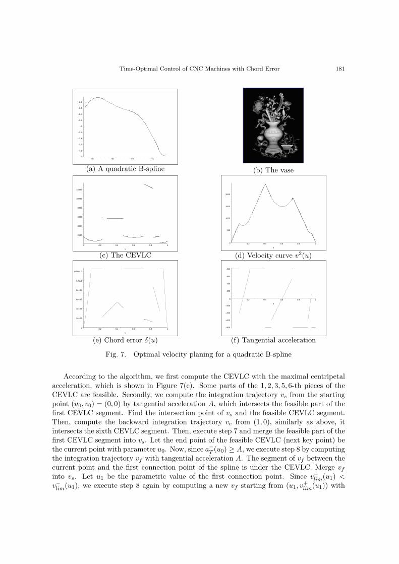
We use an example to illustrate the algorithm. The curve in Figure 7(a) is a quadraticB-spline consisting of six pieces of quadratic curve segments, which is from the tool path ofthe vase in Figure 7(b). Details of the G-codes and splines generated from the G-codes forthe vase can be found in [26]. We set the tangential and centripetal acceleration bounds tobe A = 800 mm/s2 and B = 1000 mm/s2 respectively.


–4

–3.8

–3.6

–3.4

–3.2

–3

–2.8

–2.6

–2.4

–2.2

48 49 50 51

(a) A quadratic B-spline (b) The vase

2000

4000

6000

8000

10000

12000

0 0.2 0.4 0.6 0.8 1

u

(c) The CEVLC

0

500

1000

1500

2000

0.2 0.4 0.6 0.8 1

u

(d) Velocity curve v2(u)

0

2e–05

4e–05

6e–05

8e–05

0.0001

0.00012

0.2 0.4 0.6 0.8 1

u

(e) Chord error δ(u)

–800

–600

–400

–200

0

200

400

600

800

0.2 0.4 0.6 0.8 1

u

(f) Tangential acceleration

Fig. 7. Optimal velocity planing for a quadratic B-spline

According to the algorithm, we first compute the CEVLC with the maximal centripetalacceleration, which is shown in Figure 7(c). Some parts of the 1, 2, 3, 5, 6-th pieces of theCEVLC are feasible. Secondly, we compute the integration trajectory vs from the startingpoint (u0, v0) = (0, 0) by tangential acceleration A, which intersects the feasible part of thefirst CEVLC segment. Find the intersection point of vs and the feasible CEVLC segment.Then, compute the backward integration trajectory ve from (1, 0), similarly as above, itintersects the sixth CEVLC segment. Then, execute step 7 and merge the feasible part of thefirst CEVLC segment into vs. Let the end point of the feasible CEVLC (next key point) bethe current point with parameter u0. Now, since a−T (u0) ≥ A, we execute step 8 by computingthe integration trajectory vf with tangential acceleration A. The segment of vf between thecurrent point and the first connection point of the spline is under the CEVLC. Merge vf

into vs. Let u1 be the parametric value of the first connection point. Since v+lim(u1) <

v−lim(u1), we execute step 8 again by computing a new vf starting from (u1, v+lim(u1)) with


tangential acceleration A. vf intersects the CEVLC at the second connection point of thespline. Merge vf into vs. Let u2 be the parametric value of the second connection point.Since vs(u2) > v−lim(u2), according to the algorithm, we execute step 9 of by computing thebackward integration trajectory vb from (u2, v

−lim(u2)), which intersects vs only once. Update

vs accordingly. In this way, we can obtain the final velocity curve shown in Figure 7(d),which consists of eleven pieces, where the 1, 3, 4, 5, 7, 8, 9, 11-th pieces are controlled by thetangential acceleration, and the 2, 6, 10-th pieces are feasible CEVLC segments. Figure 7(e)is the chord error of the optimal velocity curve with a sampling period T = 1ms, whichmeans d = 1.25µm. Figure 7(f) is its tangential acceleration. From these two figures, wecan see that the control is “Bang-Bang.”

Now, we give a more complicated example shown in Figure 8(a), which is a complete toolpath segment C(u) = (x(u), y(u)) of the vase in Figure 7(b) from top to bottom and consistsof 57 quadratic B-spline curve segments and 5 long straight line segments. Figure 8(b) isits velocity limited curve with centripetal acceleration B = 1000 mm/s2. Figure 8(c) isthe optimal velocity curve computed with our algorithm with tangential acceleration A =800 mm/s2 and centripetal acceleration B = 1000 mm/s2, which consists of 127 curvesegments. Figure 8(d) is the chord error of the optimal velocity curve with a samplingperiod T = 1ms, which means d = 1.25µm. Figure 8(e) is its tangential acceleration. Notethat in the connection point of a straight line segment and a quadratic B-spline, the velocitydecreases to zero.

3.2 Velocity planning for cubic PH-splines

Let C(u), u = 0..1 be a cubic PH-spline. Since a cubic PH-spline only has C1 continuity,the connection points of the PH-spline are all the key points of first or second type of theCEVLC. Let r(u) be a piece of cubic PH-curve of C(u). Then, r′(u) has the followingrepresentation [8]:

r′(u) =(f(u)2 + g(u)2 −m(u)2 − n(u)2,2(f(u)n(u) + g(u)m(u)), (12)2(g(u)n(u)− f(u)m(u))).

where f(u), g(u),m(u), n(u) are linear functions in u.The curvature of r(u) is k(u) = |r′×r′′|

σ3 = Eσ2 , where σ = |r′| = f(u)2 + g(u)2 + m(u)2 +

n(u)2 and E is a constant. The CEVLC of r(u) is

q = v2 =B

|k(u)| = Gσ2,

where G is a constant. The tangential acceleration along the CEVLC is: aT = (Gσ2)′2σ = Gσ′.

Since σ is of degree two, aT (u) is a linear function in the parameter u. The key points ofthe third type can be computed by solving linear equations aT = ±A directly.

For a cubic PH-curve, when the velocity is controlled by the tangential acceleration, theintegration trajectory is a polynomial in u with degree three. The integration trajectory isthe solution of the following differential equation:

q′ = ±2Aσ = ±2A(au2 + bu + c), (13)


(a) quadratic B-splines r(u) = (x(u), y(u))

(b) Velocity limited curve qlim(u) = v2lim(u)

(c) Velocity curve q = v2(u)

(d) Chord error δ(u)

(e) Tangential acceleration aT (u)

Fig. 8. Optimal velocity planing for quadratic B-splines from a vase

where a, b, c are constants. Let i(u) = ±2A(1/3 au3 + 1/2 bu2 + cu). Then, q(u) = i(u) −


–2

0

2

4

6

8

10

5 10 15 20 25

(a) Cubic PH-spline

5000

10000

15000

20000

25000

0 0.2 0.4 0.6 0.8 1

t

(b) The CEVLC

0

5000

10000

15000

20000

0.2 0.4 0.6 0.8 1

u

(c) Velocity q = v2(u)

0

2e–05

4e–05

6e–05

8e–05

0.0001

0.00012

0.2 0.4 0.6 0.8 1

u

(d) Chord error δ(u)

–3000

–2000

–1000

0

1000

2000

3000

0.2 0.4 0.6 0.8 1

u

(e) Tangential accelerationof velocity curve

Fig. 9. Optimal velocity planning for a cubic PH-spline

i(u∗) + q(u∗) is the solution of the differential equation (13) with initial value (u∗, q(u∗)).Now, we give an illustrative example for a cubic PH-spline (Fig. 9(a)).The cubic PH-spline consists of two pieces of PH-curves and has C1 continuity. Let the

tangential and centripetal acceleration bounds be A = 3000mm/s2 and B = 1000mm/s2

respectively. Here are the details to get the velocity curve. Firstly, we compute the CEVLCof the curve which consists of two feasible segments. So the key points are the startingpoint, the ending point, and the connection point of the spline. Let u∗ be the parametricvalue of the connection point of the spline. Secondly, we compute the integration tra-jectory vs from the starting point (u0, v0) = (0, 0) by tangential acceleration A. Sincevs(u∗) > vlim(u∗), we see that it must intersect the first CEVLC segment. Find the inter-section point (u1, vlim(u1)) of vs and the first CEVLC segment. Let [0, u1] be the defininginterval of vs. Compute the backward integration trajectory ve from the ending point (1, 0).Since v+

lim(u∗) < ve(u∗) < v−lim(u∗), ve does not intersect the second CEVLC segment. Let(u∗, ve(u∗)) be the intersection point of ve and the CEVLC and [u∗, 1] be the defining inter-val of ve. Starting from (u1, vlim(u1)), the CEVLC is feasible, we merge this feasible partof CEVLC into vs. Let (u∗, vs(u∗)) be the current point. Since vs(u∗) = v+

lim(u∗) < ve(u∗),execute step 8 by computing the integration trajectory vf which intersects ve at (u2, vf (u2)).The final velocity curve has four segments, where the 1, 3, 4-th segments are controlled bythe tangential acceleration and the 2-th piece is a feasible CEVLC segment.

The CEVLC, velocity curve , chord error and tangential acceleration of the velocity curveare shown in Figure 9, where the sampling period is T = 1ms.


4 Feed-rate override in NC-machining

During the NC-machining, there exists another constraint: the maximal feed-rate vmax. Inthis situation, all we need to do is to change the velocity curve to q∗(u) = min(q(u), vmax),where q(u) is the optimal velocity curve obtained in the preceding section. The procedureof the interpolation is as follows.

Algorithm 4.1 Interpolation algorithmInput: current parameter ui, the velocity curve q(u), maximum feed-rate vmax, and the

sampling time TOutput: the parameter of the next interpolation point ui+1

1. According to the velocity curve and the maximum feed-rate, let vi = min(√

q(ui), vmax).The step size is ∆L = vi · T .

2. According to the step size ∆L, compute the parameter of the next interpolation pointui+1([4, 21]).

Since for any parametric value u, whenever the value of q∗(u) is taken from q(u) or vmax,the left and right limitations of the tangential acceleration are satisfied. Hence, q∗(u) satisfiesthe maximum feed-rate, chord error, and tangential acceleration bounds. Furthermore, inCNC-machining, the users can change the maximum feed-rate during manufacturing, whichis called feed-rate override. Although the new feed-rate limitation is not required to respondimmediately, the real velocity should decrease to the new lower speed as soon as possible.The following algorithm solves the feed-rate override problem efficiently.

Algorithm 4.2 Feed-rate override algorithmInput: the velocity curve q(u), current parameter ui, the current feed-rate v∗, the modified

feed-rate limitation v′max;Output: the parametric values ui+1, ui+2, . . . of the interpolation points.

1 If v∗ > v′max, then let v′i = v∗ − AT , v′′i = max(v′i, v′max), vi = min(v′′i ,

√q(ui)). Find

the next interpolation point ui+1 according to Algorithm 4.1, i = i + 1, v∗ = vi, andrepeat step 1;

2 If v∗ ≤ v′max, then let vi = min(√

q(ui), v′max, v∗ + AT ). Find the next interpolationpoint ui+1 according to Algorithm 4.1. If ui+1 > 1, then let ui+1 = 1 and terminate;else let i = i + 1, v∗ = vi, and repeat step 2.

Since the final velocity is under the CEVLC, the error bound is satisfied. Step 1 of theabove algorithm is to slow down feed-rate as soon as possible when the current feed-rate islarger than the modified feed-rate. Step 2 of the above algorithm is exactly Algorithm 4.1,where the maximum feed-rate is replaced by the modified feed-rate.

One advantage of the algorithm presented in this paper is that feed-rate override can becarried out easily. In the case of multi-axis acceleration mode, when the maximal feed-rateis changed to vmax, we cannot simply take q∗(u) = min(q(u), vmax) to be the new velocitycurve.


5 Conclusion

In this paper, we give the first time-optimal velocity planning method for parametric curveswith confined chord error. We adopt the simplest acceleration mode: the linear accelerationfor tangential accelerations. With the method introduced in this paper, it is not difficultto give time-optimal velocity planning method with confined chord error and multi-axisacceleration modes.

The key idea is to reduce the chord error bound to a centripetal acceleration bound.When the centripetal acceleration reaches its bound, the velocity curve is an algebraic curveand is called the CEVLC. With the CEVLC, the final velocity curve is the minimum ofall the integration velocity curves starting from the key points of the CEVLC the startingpoint, and the ending point. We also give a practical algorithm to compute the time-optimalvelocity curve and implemented the algorithm for two types of curves.

References

[1] D. Bedi, I. Ali, N. Quan. Advanced techniques for CNC machines, Journal of Enginerringfor Industry, 115, 329-336, 1993.

[2] G. Birkhoff, G. Rota. Ordinary differential equations. Newyork, Blaisdell, 1969.

[3] J.E. Bobrow, S. Dubowsky, J.S. Gibson. Time-optimal control of robotic manipulatorsalong specified paths. Int. J. Robot. Res., 4(3), 3-17, 1985.

[4] C.W. Cheng, M.C. Tsai. Real-time variable feed rate NURBS curve interpolator for CNCmachining. Int. J. Adv. Manuf. Technol., 23, 865-873, 2004.

[5] J.J. Chou and D.C.H. Yang. Command generation for three-axis CNC machining. Journalof Engineering for Industry, 113, 305-310, 1991.

[6] M.M. Emami, B. Arezoo. A look-ahead command generator with control over trajectoryand chord error for NURBS curve with unknown arc length. Computer-Aided Design,4(7), 625-632, 2010.

[7] K. Erkorkmaz, Y. Altintas. High speed CNC system design. Part I: jerk limited trajectorygeneration and quintic spline interpolation. Int. J. of Mach. Tools and Manu., 41, 1323-1345, 2001.

[8] R.T. Farouki. Pythagorean-hodograph curves, Springer, Berlin, 2008.

[9] R.T. Farouki, Y.F. Tsai. Exact Taylor series coefficients for variable-feedrate CNC curveinterpolators. Computer-Aided Design, 33(2), 155-165, 2001.

[10] J.Y. Lai, K.Y. Lin, S.J. Tseng, W.D. Ueng. On the development of a parametric inter-polator with confined chord error, feedrate, acceleration and jerk. Int. J. Adv. Manuf.Technol. , 37: 104C121, 2008.


[11] M.T. Lin, M.S. Tsai, H.T. Yau. Development of a dynamics-based NURBS interpolatorwith real-time look-ahead algorithm. Int. J. of Mach. Tools and Manu., 47(15), 2246-2262, 2007.

[12] S. Macfarlane, E.A. Croft. Jerk-bounded manipulator trajectory planning: design forreal-time applications. IEEE Trans. on Robot. and Automa., 19: 42-52, 2003.

[13] S.H. Nam, M.Y. Yang. A study on a generalized parametric interpolator with real-timejerk-limited acceleration. Computer-Aided Design 36, 27-36, 2004.

[14] J. Park, S.H. Nam, M.Y. Yang. Development of a real-time trajectory generator forNURBS interpolation based on the two-stage interpolation method. Int. J. Adv. Manuf.Technol., 26: 359-365, 2005.

[15] Z. Shiller. On singular time-optimal control along specified paths. IEEE Trans. Robot.Autom., 10, 561-566, 1994.

[16] Z. Shiller, H.H. Lu. Robust computation of path constrained time optimal motions.Proc., IEEE Inter. Conf. on Robot. Autom., Cincinnati, OH, 144-149, 1990.

[17] K.G. Shin, N.D. McKay. Minimum-time control of robotic manipulators with geometricpath contraints. IEEE Trans. on Automatic Control, 30(6), 531-541, 1985.

[18] M. Shpitalni, Y. Koren, C.C. Lo. Realtime curve interpolators. Computer-Aided Design26(1), 832-838, 1994.

[19] S.D. Timar, R.T. Farouki, T.S. Smith, C.L. Boyadjieff. Algorithms for time-optimalcontrol of CNC machines along curved tool paths. Robotics and Computer-IntegratedManufacturing, 21(1), 37-53, 2005.

[20] S.D. Timar, R.T. Farouki. Time-optimal traversal of curved paths by Cartesian CNCmachines under both constant and speed-dependent axis acceleration bounds. Roboticsand Computer-Integrated Manufacturing, 23(5), 563-579, 2007.

[21] Z.M. Xu, J.C Chen and Z.J Feng. Performance Evaluation of a Real-Time InterpolationAlgorithm for NURBS Curves. Int. J. Adv. Manuf. Technol., 20: 270-276, 2002.

[22] D.C.H. Yang, T. Kong. Parametric interpolator versus linear interpolator for precisionCNC machining. Computer-Aided Design, 26(3), 225-234, 1994.

[23] S.S. Yeh, P.L. Hsu. Adaptive-feedrate interpolation for parametric curves with a confinedchord error. Computer-Aided Design, 34, 229-237, 2002.

[24] T. Yong, R. Narayanaswami. A parametric interpolator with confined chord errors,acceleration and deceleration for NC machining. Computer-Aided Design, 35, 1249-1259,2003.

[25] K. Zhang, X.S. Gao, H. Li, C.M. Yuan. A greedy algorithm for feed-rate planning ofCNC machines along curved tool paths with jerk constraints. MM Research Preprints,29, 189-205, 2010.


[26] M. Zhang, W. Yan, C.M. Yuan, D. Wang, X.S. Gao. Curve fitting and optimal in-terpolation on CNC machines based on quadratic B-splines(in Chinese). MM ResearchPreprints, 29, 71-91, 2010.

Time-Optimal Interpolation of CNC Machines along ...xgao/papernc/29-09.pdf · Time-Optimal Interpolation of CNC Machines ... @mmrc.iss.ac.cn. ... optimal velocity planning method

Documents