Time of Events in Quantum Theory1 - CORE

Preprint No BiBoS 720/1/96

Time of Events in Quantum Theory1

Ph. Blanchard[2 and A. Jadczyk]3

[ Faculty of Physics and BiBoS, University of Bielefeld

Universit�atstr. 25, D-33615 Bielefeld] Institute of Theoretical Physics, University of Wroc law

Pl. Maxa Borna 9, PL-50 204 Wroc law

Abstract

We enhance elementary quantum mechanics with three simple pos-

tulates that enable us to de�ne time observable. We discuss shortly

justi�cation of the new postulates and illustrate the concept with the

detailed analysis of a delta function counter.

1This paper is dedicated to Klaus Hepp and to Walter Hunziker on the occasion of

their sixtieth anniversary2e-mail: [email protected]: [email protected]

brought to you by COREView metadata, citation and similar papers at core.ac.uk

provided by CERN Document Server

Zeit ist nur dadurch, da� etwas geschieht

und nur dort wo etwas geschiecht.

(E.Bloch)

1 Introduction

Time plays a peculiar role in Quantum Mechanics. It di�ers from other

physical quantities like position or momentum. When discussing position a

dialogue may look like this: 4

SP: What is the position?

SG: Position of what?

SP: Of the particle.

SG: When?

SP: At t=t1.

SG: The answer depends on how you are going to measure this position.

Are you sure you have detectors put everywhere that interact with the par-

ticle only during the time interval (t-dt,t+dt) and not before?

When talking about time we will have something like this:

SP: What is time?

SG: Time of what?

SP: Time of a particle.

SG: Time of your particle doing what?

SP: Time of my particle leaving the box where it was trapped. Or time

at which my particle enters the box.

SG: Well, it depends on the box and it depends on the method you want

to apply to ascertain that the event has happened.

SP: Why can't we simply put clocks everywhere, as it is common in

discussions of special relativity? And let these clocks note the time at which

the particle passes them?

SG: Putting clocks disturbs the system. The more clocks you put - the

more you disturb. If you put them everywhere - you force wave packet

reductions a'la GRW. If you increase their time resolution more and more

- you increase the frequency of reductions. When the clocks have in�nite

4We use the method chosen by Galileo in his great book "Dialogues Concerning Two

New Sciences"[1]. Galileo is often refered to as the founder of modern physics. The most

far{reaching of his achievements was his counsel's speech for mathematical rationalism

against Aristotle's logico{verbal approach, and his insistence for combining mathematical

analysis with experimentation.

In the dialog SG=Sagredo, SV=Salviati, SP=Simplicio

1

resolutions - then the particle stops moving - this is the Quantum Zeno e�ect

[2].

SP: I do not believe these wave packet reductions. Zeh published a

convincing paper whose title tells its content: "There are no quantum jumps

nor there are particles" [3], and Ballentine [4, 5], proved that the projection

postulate is wrong.

SG I remember these papers. They had provocative titles...

SV. First of all Ballentine did not claim that the projection postulate is

wrong. He said that if incorrectly applied - then it leads to incorrect results.

And indeed he showed how incorrect application of the projection postulate

to the particle tracks in a cloud chamber leads to inconsistency. What he

said is this: "According to the projection postulate, a position measurement

should "collapse" the state to a position eigenstate, which is spherically

symmetric and would spread in all directions, and so there would be no

tendency to subsequently ionize only atoms that lie in the direction of the

incident momentum. An approximate position measurement would similarly

yield a spherically symmetric wave packet, so the explanation fails." This is

exactly what he said. And this is correct. This shows how careful one has to

be with the projection postulate. If the projection postulate is understood

as operating with an operator on a state vector: �! R =kR k, then the

argument does not apply. Thus a correct application would be to multiply

the moving Gaussian of the particle, something like:

(x; t) = exp(ip(x� a(t)) exp(�(x� a(t))2=�(t))

which is spherically symmetric, but only up to the phase, by a static Gaus-

sian modelling a detector localized around a:

f(x) = exp(��(x� a)2)

The result is again a moving Gaussian. And in fact, such a projection pos-

tulate is not a postulate at all. It can be derived from the simplest possible

Liouville equation.

SP: Has this "correct", as you claim, cloud chamber model been pub-

lished? Have its predictions been experimentally veri�ed?

SV: A general theory of coupling between quantum system and a clas-

sical one is now rather well understood [6]. The cloud chamber model has

been published quite recently, you can take a look at [7, 8]. Belavkin and

Melsheimer [9] tried to derive somewhat similar result from a pure unitary

evolution, but I am not able to say what assumptions they used, what ap-

proximations they made and what exactly are their results.

SP: Didn't the problem was solved long ago in the classical paper by

Mott [10]?

2

SV Mott did not even attempted to derive the timing of the tracks. In the

cloud chamber model of Refs. [7, 8], that I understand rather well, because

I participated in its construction, it is interesting that the detectors { even if

they do not "click" { in uence the continuous evolution of the wave packet

between reductions. They leave a kind of a "shadow". This is another case

of a "interaction-free" experiment discussed by Dicke [11, 12], and then by

Elitzur and Vaidman [13] in their "bomb{test" allegory, and also by Kwiat,

Weinfurter, Herzog and Zeilinger [14]. The shadowing e�ect predicted by

EEQT 5 may be tested experimentally. I believe it will �nd many applica-

tions in the future, and I hope these will be not only the military ones! Yet

we must now not digress upon this particular topic since you are waiting

to hear what I think about the problem of time in quantum theory. We

already know that "time" must be "time of something". Time of something

that happens. Time of some event.6But in quantum theory events are not

simply space-time events as it is in relativity. Quantum theory is speci�c in

the sense that there are no events unless there is something external to the

quantum system that "causes" these events. And this something external

must not be just another quantum system. If it is just another quantum

system - then nothing happens, only the state vector continuously evolves

in parameter time.

SP But is it not so that there are no sharp events? Nothing is sharp,

nothing really sudden. All is continuous. All is approximate.

SG How nothing is sharp, do we not register "clicks" when detecting

particles?

SP I do not know what clicks are you talking about ...

SG How you don't know? Ask the experimentalist.

SP I am an experimentalist!

SV The problem you are discussing is not an easy one to answer. I

pondered on it many times, but did not arrive at a clear conclusion. Never-

theless something can be said with certainty. First of all you both agree that

in physics we always have to deal with idealizations. For instance one can

argue that there are no real numbers, that the only, so to say, experimental

numbers are the natural numbers. Or at most rational numbers. But real

numbers proved to be useful and today we are open to both possibilities: of

a completely discrete world, and of a continuous one. Perhaps there is also

a third possibility: of a fuzzy world. Similarly there are di�erent options

for modelling the events. One can rightly argue that they are never sharp.

But do they happen or not? Do we need counting them? Do we need a

5Salviatti refers here to "Event Enhanced Quantum Theory" of reference [6] - paper

apparently well know to the participants of the dialog.6Heisenberg proposed the word "event" to replace the word "measurement", the latter

word carrying a suggestion of human involvement.

3

theory that describes these counts? We do. So, what to do? We have no

other choice but to try di�erent mathematical models and to see which of

them better �t the experiment, better �t the rest of our knowledge, better

explain what makes Nature tick. In the cloud chamber model that we were

talking about just a while ago the events are unsharp in space but they are

sharp in time. And the model works quite well. However, if you try to work

out a relativistic cloud chamber model, then you see that the events must

be also smeared out in the coordinate time.7 Nevertheless they can still be

sharp in a di�erent "time", called "proper time" after Fock and Schwinger.

If time allows I will tell you more about this relativistic theory, but now let

us agree that in a nonrelativistic theory sharp localization of events in time

does not contradict any known principles. We will remember at the same

time that we are dealing here with yet another idealization that is good as

long as it works for us. And we must not hesitate to abandon it the moment

it starts to lead us astray. The principal idea of EEQT is the same as that

expressed in a recent paper by Haag [16]. Let me quote only this: "... we

come almost unavoidably to an evolutionary picture of physics. There is an

evolving pattern of events with causal links connecting them. At any stage

the `past' consists of the part which has been realized, the `future' is open

and allows possibilities of new events ..."

SG Let me interrupt you. Perhaps we should remember what Bohr was

telling us. Bohr insisted that the apparatus has to be described in terms

of classical physics; this point of view is a common{place for experimental

physicists. Indeed any experimental article observes this rule. This principle

of Bohr is not in any way a contradiction but simply the recognition of the

fact that any physical theory is always the expression of an approximation

and an idealization. Physics is always a little bit false. Epistemology must

also play role in the labs. Physics is a system of analogies and metaphors.

But these metaphors are helping us to understand how Nature does what it

does.

SP I agree with this. So what is your proposal? How to describe time

of events in a nonrelativistic quantum theory? Do one �rst have to learn

EEQT - your "Event Enhanced Quantum Theory" that you are so proud

of? I know many theoretical physicists dislike your explicit introduction of a

classical system. They prefer to keep everything classical in the background.

Never put it into the equations.

SV Here we have a particularly lucky situation. For this particular purpose

of discussing time of events it is not necessary to learn EEQT. It is possible

to describe time observation with simple rules. This is normal in standard

quantum mechanics. You are told the rules, and you are told that they

7Cf. an illuminating discussion of this point in [15].

4

work. So you believe them and you are happy that you were told them. In

EEQT Schr�odinger's evolution and reduction of the wave function appear

as special cases of a single law of motion which governs all systems equally.

EEQT is one of the few approaches that allow you to derive quantum me-

chanical postulates and to see that these postulates re ect only part of the

truth. Here, when discussing time of events we do not need the full predic-

tive power of EEQT. This is so because after an event has been registered

the experiment is over. We are not interested here in what happens to our

system after that. Therefore we need not to speak about jumps and wave

packet reductions. It is only if you want to derive the postulates for time

measurements, only then you will have to look at EEQT. But instead of

deriving the rules, it is even better to see if they give experimentally valid

predictions. We know too many cases where good formulas were produced

by doubtful methods and bad formulas with seemingly good ones. Using

the right tool makes the job easier.

SP I become impatient to see your postulates, and to see if I can accept

them as reasonable even before any experimental testing. Only if I see that

they are reasonable, only then I will have any motivation to see whether

they really be derived from EEQT, or perhaps in some other way.

2 Time of Events

We start our discussion on quite a general and somewhat abstract level.

Only later on, in examples, we will specialize both: our system and the

monitoring device. We consider quantum system described by a Hilbert

space H. 8 To answer the question "time of what?", we must select a prop-

erty of the system that we are going to monitor. It must give only "yes-no",

or one-zero answers. We denote this binary variable with the letter �. In our

case, starting at t = 0, when the monitoring begins, we will get continuously

� = 0 reading on the scale, until at a certain time, say t = t1, the reading

will change into "yes". Our aim is to get the statistics of these "�rst hitting

times", and to �nd out its dependence of the initial state of the system and

on its dynamics.

Speaking of the "time of events" one can also think that "events" are tran-

sitions which occur; sometimes the system is changing its state randomly

- and these changes are registered. There are two kinds of probabilities in

Quantum Mechanics the transition probabilities and another probabilities

- those that tell us when the transitions occur. It is this second kind of

8More generally we would need two Hilbert spaces: Hno and Hyes that can be di�erent,

but for the present discussion we need not be pedantic, so we will assume them to be

identi�ed.

5

probabilities that we will discuss now.

2.1 First Postulate - the Coupling

Our �rst postulate reads: the coupling to a "yes-no" monitoring device is

described by an operator � � 0 in the Hilbert space H. In general � may

explicitly depend on time but here, for simplicity, we will assume that this is

not the case. That means: to any real experimental device there corresponds

a �. In practice it may be di�cult to produce the � that describes exactly

a given device. Like it is di�cult to �nd the Hamiltonian that takes into

account exactly all the forces that act in a system. Nevertheless we believe

that an exact Hamiltonian exists, even if it is hard to �nd or impractical

to apply. Similarly our postulate states that an exact � exists, although it

may be hard to �nd or impractical to apply. Then we use an approximate

one, a model one.

It should be noticed that we do not assume that � is an orthogonal

projection. This re ects the fact that our device - although giving de�nite

"yes-no" answers, gives them acting upon possibly fuzzy criteria. In the

limit when the criteria become sharp one should think of � as � �! �E,

where � is a coupling constant of physical dimension t�1 and E a projection

operator. In general case it is usually convenient to write � = ��0; where

�0 is dimensionless.

It is also important to notice that the property that is being monitored

by the device need not be an elementary one. Using the concepts of quantum

logic (cf. [17, 18]) the property need not be atomic - it can be a composite

property. In such a case, when thinking about physical implementation of

the procedure determining whether the property holds or no, there are two

extreme cases. Roughly speaking the situation here is similar to that occur-

ring in discussion of superpositions of state preparation procedures. Some

procedures lead to a coherent superpositions, some other lead to mixtures.

Similarly with composite detectors: one possibility is that we have a dis-

tributed array of detectors that can act independently one of another, and

our event consists on activating one of them. Another possibility is that we

have a coherent distributed detector like a solid state lattice that acts as

one detector. In the �rst case (called incoherent) � will be of the form

� =X�

g?�g�;

while in the second coherent case:

� = (X�

g�)?(X�

g�);

6

where g� are operators associated to individual constituents of the detector's

array. More can be said about this important topic, but we will not need to

analyze it in more details for the present purpose.

2.2 Second Postulate - the Probability

We assume that, apart of the monitoring device, our system evolves under

time evolution described by the Schr�odinger equation with a self{adjoint

Hamiltonian H0 = H?0 . We denote by K0(t) = exp(�iH0t) the correspond-

ing unitary propagator. Again, for simplicity, we will assume that H0 does

not depend explicitly on time.

Our second postulate reads: assuming that the monitoring started at

time t = 0, when the system was described by a Hilbert space vector 0,

k 0k = 1, and when the monitoring device was recording the logical value

"no", the probability P (t) that the change no ! yes will happen before

time t is given by the formula:

P (t) = 1� k tk2; (1)

where

t = K(t) 0 (2)

and

K(t) = exp(�iH0t ��t

2): (3)

Remark: The factor 12in the formula above is put here for consistency with

the notation used in our previous papers.

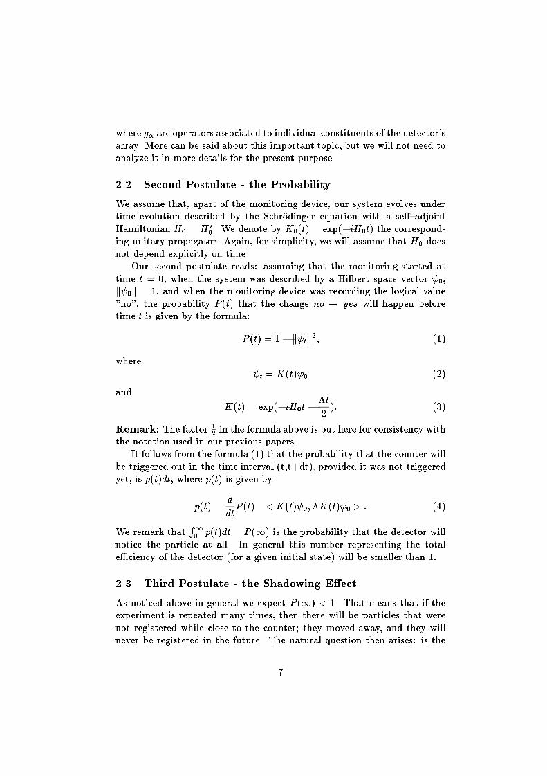
It follows from the formula (1) that the probability that the counter will

be triggered out in the time interval (t,t+dt), provided it was not triggered

yet, is p(t)dt, where p(t) is given by

p(t) =d

dtP (t) =< K(t) 0;�K(t) 0 > : (4)

We remark thatR10 p(t)dt = P (1) is the probability that the detector will

notice the particle at all. In general this number representing the total

e�ciency of the detector (for a given initial state) will be smaller than 1:

2.3 Third Postulate - the Shadowing E�ect

As noticed above in general we expect P (1) < 1. That means that if the

experiment is repeated many times, then there will be particles that were

not registered while close to the counter; they moved away, and they will

never be registered in the future. The natural question then arises: is the

7

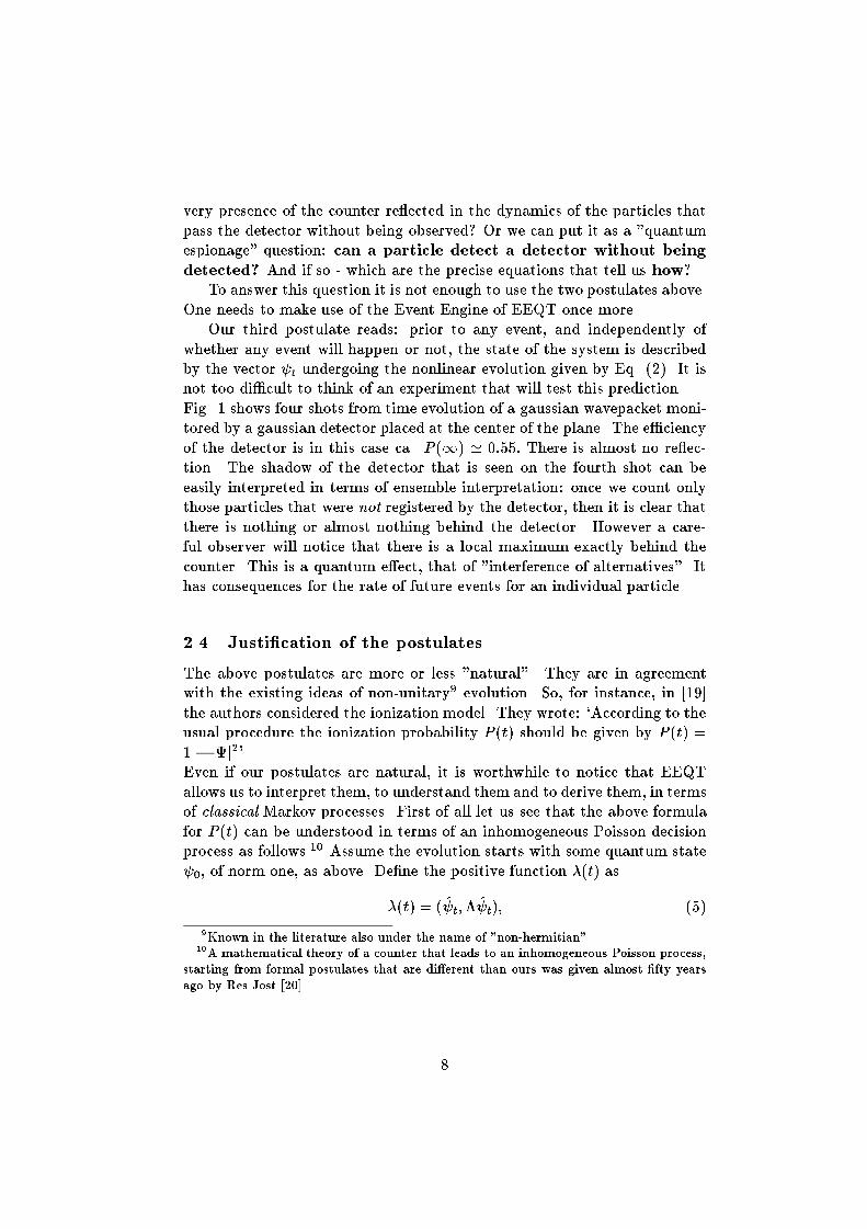
very presence of the counter re ected in the dynamics of the particles that

pass the detector without being observed? Or we can put it as a "quantum

espionage" question: can a particle detect a detector without being

detected? And if so - which are the precise equations that tell us how?.

To answer this question it is not enough to use the two postulates above.

One needs to make use of the Event Engine of EEQT once more.

Our third postulate reads: prior to any event, and independently of

whether any event will happen or not, the state of the system is described

by the vector t undergoing the nonlinear evolution given by Eq. (2). It is

not too di�cult to think of an experiment that will test this prediction.

Fig. 1 shows four shots from time evolution of a gaussian wavepacket moni-

tored by a gaussian detector placed at the center of the plane. The e�ciency

of the detector is in this case ca. P (1) ' 0:55: There is almost no re ec-

tion. The shadow of the detector that is seen on the fourth shot can be

easily interpreted in terms of ensemble interpretation: once we count only

those particles that were not registered by the detector, then it is clear that

there is nothing or almost nothing behind the detector. However a care-

ful observer will notice that there is a local maximum exactly behind the

counter. This is a quantum e�ect, that of "interference of alternatives". It

has consequences for the rate of future events for an individual particle.

2.4 Justi�cation of the postulates

The above postulates are more or less "natural". They are in agreement

with the existing ideas of non-unitary9 evolution. So, for instance, in [19]

the authors considered the ionization model. They wrote: `According to the

usual procedure the ionization probability P (t) should be given by P (t) =

1� jj2'.Even if our postulates are natural, it is worthwhile to notice that EEQT

allows us to interpret them, to understand them and to derive them, in terms

of classical Markov processes. First of all let us see that the above formula

for P (t) can be understood in terms of an inhomogeneous Poisson decision

process as follows.10 Assume the evolution starts with some quantum state

0, of norm one, as above. De�ne the positive function �(t) as

�(t) = ( t;� t); (5)

9Known in the literature also under the name of "non-hermitian"10A mathematical theory of a counter that leads to an inhomogeneous Poisson process,

starting from formal postulates that are di�erent than ours was given almost �fty years

ago by Res Jost [20] .

8

where

t = t

k tk; : (6)

Then P (t) above happens to be nothing but the �rst-jump probability of

the inhomogeneous Poisson process with intensity �(t). It is instructive to

see that this is indeed the case. To this end let us divide the interval (0; t)

into n subintervals of length �t = t=n. Denote tk = (k� 1)�t; k = 1; : : : ; n:

The inhomogeneous Poisson process of intensity �(t) consists then of taking

independent decisions `jump{or{not{jump' in each time subinterval.

Probability for jumping in the k-th subinterval is assumed to be pk =

�(tk�1)�t (that is why � is called the intensity of the process). Thus the

probability Pnot(t) of not jumping up to time t is

Pnot(t) = limn!1

nYk=1

(1� pk) = exp(�Z t

0

�(s)ds): (7)

Let us show that 1 � Pnot(t) can be identi�ed with P (t) given by Eq. (7).

To this end notice that

d

dt(1� P (t)) = � < t;� t >= ��(t)k tk2

= ��(t)(1� P (t)):

Thus 1 � P (t), given by Eq. (1) satis�es the same di�erential equation

as Pnot(t) given by Eq. (7). Because 1 � P (0) = Pnot(0) = 1, it follows

that 1 � P (t) = Pnot(t), and so P (t) = 1� Pnot(t) indeed is the �rst jump

probability of the inhomogeneous Poisson process with intensity �(t).

This observation is useful but rather trivial. It can not yet stand for a

justi�cation of the formula (1) - this for the simple reason that the jump

process above, based upon a continuous observation of the variable � and

registering the time instant of its jump, is not a Markovian process. It

would become Markovian if we know �(t), but to know �(t) we must know

t. This leads us to consider pairs xt = ( t; �t), where t is the Hilbert

space vector describing quantum state, and �t is the yes-no state of the

counter. Then t evolves deterministically according to the formula (2), the

intensity function �(t) is computed on the spot, and the Poisson decision

process described above is responsible for the jump of value of � - in our

case it corresponds to a "click" of the counter. The time of the click is a

random variable T1, well de�ned and computable by the above prescription.

This prescription sheds some light onto the meaning of the quantum state

vector . We see that codes in itself information that is being used

by a decision mechanism working in an entirely classical way - the only

9

randomness we need is that of a biased (by �(t)) classical roulette. Until we

ask why the bias is determined by this particular functional of the quantum

state, until then we do not have to invoke more esoteric concepts of quantum

probability { whatever they mean. But, in fact, it is possible to understand

somewhat more, still in pure classical terms. We will not need this extra

knowledge in the rest of this paper, but we think it is worthwhile to sketch

here at least the idea.

In the reasoning above we were interested only in what governs the time of

the �rst jump, when the counter clicks. But in reality nothing ends with this

click. Photon, for instance, when detected, is transformed into another form

of energy. So, if we want to continue our process in time, after T1, we must

feed it with an extra information: how is the quantum state transformed as

the result of the jump. So, in general, we have a classical variable � that

can take �nitely many, denumerably many, a continuum, or more, possible

values, and to each ordered pair (� ! �) there corresponds an operator

g��. The transition (� ! �) is called an event, and to each event there

corresponds a transformation of the quantum state ! g�� kg�� k

. In the case

of a counter there is only one �. In general, when there are several �-s, we

need to tell not only when to jump, but also where to jump. One obtains

in this way a piecewise deterministic Markov process on pure states of the

total system: (quantum object, classical monitoring device). It can be then

shown [6, 21] that this process, including the jump rate formula (5) follows

uniquely from the simplest possible Liouville equation that couples the two

systems.

3 The Time of Arrival

As the most natural application of the above concept of "time of event"

we consider the notion of "time of arrival" of a particle to a certain state.

There are several methods available for computing the "time of arrival"

distribution given our postulates. We shall take the approach that seems to

us to be the simplest one. One by one we shall specialize our assumptions

about �.

3.1 One elementary detector

Let K(t) be given by Eq. (3), and let

K0(t) = exp(�iH0t): (8)

Then K(t) satis�es the Schr�odinger equation

_K = �iH0K(t)� �

2K(t): (9)

10

This di�erential equation, together with initial data K(0) = I , is easily

seen to be equivalent to the following integral equation:

K(t) = K0(t)�1

2

Z t

0

K0(t � s)�K(s)ds: (10)

By taking the Laplace transform and by the convolution theorem we get the

Laplace transformed equation:

~K = ~K0 �1

2~K0� ~K: (11)

Let us consider the case of a maximally sharp measurement. In this case we

would take � = ja >< aj, where ja > is some Hilbert space vector. It is not

assumed to be normalized; in fact its norm stands for the strength of the

coupling (notice that < aja > must have physical dimension t�1). Taking

look at the formula (4) we see that now p(t) = j < aj t > j2 and so we need

to know < ajK(t) 0 > rather than the full propagator K(t). Multiplying

Eq. (11) from the left by < aj and from the right by j 0 > we obtain:

< aj ~ >= 2 < aj ~K0j 0 >2 + < aj ~K0ja >

(12)

where ~ is the Laplace transform of t! (t) :

~ (z) =

Z 1

0

e�tz (t)dt = ~K(z) 0; <(z) � 0: (13)

3.2 Composite detector

We consider now the simplest case of a composite detector. It will be an

incoherent composition of two simple ones. Thus we will take:

� = ja1 >< a1j+ ja2 >< a2j: (14)

Remark Notice that if < a1ja2 >= 0, then coherent and incoherent compo-

sitions are indistinguishable, as in this case, with gi = jai >< aij; we havethat

Pi gi

?gi = (Pi gi)

?(Pi gi):

For p(t) we have now the formula:

p(t) =Xi

j < aij t > j2; (15)

and to compute the complex amplitudes < aij t > we will use the Laplace

transform method as in the case of one detector. To this end one applies

11

< aij from the left and j 0 > from the right to Eq. (11) and solves the

resulting system of two linear equations to obtain:

< a1j ~ > = 2�

((2 + (22)) < a1j ~ 0 > �(12) < a2j ~ 0 > )

< a2j ~ > = 2�

((2 + (11)) < a2j ~ 0 > �(21) < a1j ~ 0 > )

9>=>; (16)

where we used the notation

(ij) =< aij ~K0jaj >; (17)

j ~ 0 >= ~K0j 0 >; (18)

and where � stands for

� = 4+ 2((11)+ (22))+ ((11)(22)� (12)(21)): (19)

The probability density p(t) is then given by

p(t) =Xi

j�i(t)j2; (20)

where �i is the inverse Fourier transform

�i(t) =1

2�

Z 1

�1eity ~�i(iy)dy (21)

of~�i(iy) = lim

x=0+< aij ~ (x+ iy) > : (22)

By the Parseval formula we have that P (1) is given by:

P (1) =1

2�

Xi

Z 1

�1j~�i(iy)j2dy : (23)

3.3 Example: Dirac's � counter for ultra-relativistic particle

Let us now specialize the model by assuming that we consider a particle in

R1 and that the Hilbert space vector ja > approaches the improper position

eigenvectorp��(x�a) localized at the point a. This corresponds to a point{

like detector of strength � placed at a.11 We see from the equation (4) that

p(t) is in this case given by:

p(t) = j�(t)j2; (24)

11The case of Hermitian singular delta{function perturbation was discussed by many

authors - see [22, 23, 24, 25, 26, 27, 28] and references therein

12

where the complex amplitude �(t) of the particle arriving at a is:

�(t) =< aj (t) >; (25)

or, from Eq. (12)

~� =2p�

2 + � ~K0(a; a)~ 0(a) (26)

where ~ 0 stands for the Laplace transform of K0(t) 0.

Let us now consider the simplest explicitly solvable example - that of an

ultra{relativistic particle on a line. For H0 we take H0 = �ic ddx ; then the

propagator K0 is given by K0(x; x0; t) = �(x0 � x + ct); and its Laplace

transform reads ~K0(x; x0; z) = 1

c e(x�x0)z=c. In particular ~K0(a; a; z) =

1c and

from Eq. (26) we see that the amplitude for arriving at the point a is given

by the "almost evident" formula:

�(t) = const(�)� (a� ct); (27)

where const(�) =p�=(1 + �

2c): It follows that probability that the particle

will be registered is equal to

P (1) =�=c

(1 + �2c)

2

Z a

�1dxj 0(x)j2 (28)

which has a maximum P (1) = 1=2 for � = 2c if the support of 0 is left

to the counter position a: We notice that in this example the shape of the

arrival time probability distribution p(t) does not depend on the value of

the coupling constant - only the e�ectiveness of the detector depends on it.

For a counter corresponding to a superpositionPip�i�(x � ai) we obtain

for P (1) exactly the same expression as for one counter but with � replaced

withPi �i:

3.4 Example: Dirac's � counter for Schr�odinger's particle

We consider now another example corresponding to a free Schr�odinger's

particle on a line. We will study response of a Dirac's delta counter ja >=p��(x� a), placed at x = a, to a Gaussian wave packet whose initial shape

at t = 0 is given by:

0(x) =1

(2�)1=4�1=2exp

�(x � x0)2

4�2+ 2ik(x� x0)

!: (29)

In the following it will be convenient to use dimensionless variables for mea-

suring space, time and the strength of the coupling:

� =x

2�; � =

�ht

2m�2; � =

m��

�h(30)

13

We denote

�0 = x0=2�; �a = a=2�; v = 2�k (31)

In these new variables we have:

0(�) =�2�

�1=4e�(���0)

2+2iv(���0) (32)

K0(�0; �; �) =

�1�i�

�1=2exp

�i(�0��)2

�

�(33)

~K0(�0; �; z) = (iz)�

1

2 exp��2p�iz j�0 � �j

�(34)

We can compute now explicitly ~ (z) of Eq. (13):

~ 0(a; z) =

��

2

�1=4(iz)�1=2e�d

2�2ivd [w(u+) + w(u�)] (35)

where

u� = ip�iz � (v � id); d = �0 � �a; (36)

and the amplitude ~� of Eq. (26) reads

~�(z) =1

2(2�)1=4�1=2e�d

2�2ivd w(u+) + w(u�)

2piz + �

(37)

with the function w(z) de�ned by

w(u) = e�u2

erfc(�iu) (38)

(see Ref. [29], Ch. 7.1.1 { 7.1.2). We have also used the formula

Z 1

0

exp��ax2 + 2bx+ c

�dx =

1

2

r�

aexp

b2 � aca

!erfc

�bpa

�(39)

valid for <(a) > 0 (see [29], Ch. 7.4.2).

To compute p(t) from Eqs. (20,21) the correct boundary values of the com-

plex square root must be taken. Thus for z = x + iy; x = 0+ we should

take

piz =

(ipy y � 0p�y y � 0

(40)

p�iz =

( py y � 0

�ip�y y � 0(41)

The time of arrival probability curves of the counter for several values of

the coupling constant are shown in Fig.2. The incoming wave packet starts

14

at t = 0, x = �4, with velocity v = 4: It is seen from the plot that the

average time at which the counter, placed at x = 0, is triggered is about

one time unit, independently of the value of the coupling constant. This

numerical example shows that our model of a counter serves can be used for

measurements of time of arrival. It is to be noticed that the shape of the

response curve is almost insensitive to the value of the coupling constant.

Fig.3 shows the curves of Fig.2, but rescaled in such a way that the proba-

bility P (1) = 1. The only e�ect of the increase of the coupling constant in

the interval 0:01�100 is a slight shift of the response time to the left - which

is intuitively clear. Notice that the shape of the curve in time corresponds

well to the shape of the initial wave packet in space.

For a given velocity of the packet there is an optimal value of the cou-

pling constant. In our dimensionless units it is �opt � 2v. Figure 4 shows

this asymptotically linear dependence. At the optimal coupling the total

response probability P (1) approaches the value 0:5; - the same as in the

ultra{relativistic case.

By numerical calculations we have found that the maximal value of P (1)

that can be obtained for a single Dirac's delta counter and Schr�odinger's

particle is slightly higher than 0:7; that corresponds to the value � = 1:3 of

the coupling constant. The dependence of P (1) on the coupling constant

for a static wave packet (that is v = 0) centered exactly over the detector is

shown in Fig.5. Fig.6 shows the dependence of P (1) on both variables: v

and �:

The value 0:7 for the maximal response probability P (1) of a detector

may appear to be rather strange. It is however connected with the point{

like structure of the detector in our simple model. For a composite detector,

for instance already for a two{point detector, this restriction does not apply

and P (1) arbitrarily close to 1:0 can be obtained. Our method applies as

well to detectors continuously distributed in space. In this case the e�ciency

of the detector (for a given initial wavepacket) will depend on the shape of

the function �(x). The absorptive complex potentials studied in [30, 31] are

natural candidates for providing maximal e�ciency as measured by P (1)

de�ned at the end of Sec. 2.2.

4 Concluding Remarks

Our approach to the quantum mechanical measurement problem was origi-

nally shaped to a large extent by the important paper by Klaus Hepp [32].

He wrote there, in the concluding section: `The solution of the problem of

measurement is closely connected with the yet unknown correct description

of irreversibility in quantum mechanics...'Our approach does not pretend to

15

give an ultimate solution. But it attempts to show that this "correct de-

scription" is, perhaps, not too far away.

In the present paper we have only been able to scratch the surface of some

of the new mathematical techniques and physical ideas that are enhancing

quantum theory in the framework of EEQT, that free the quantum the-

ory from the limitations of the standard formulation. For a long time it

was considered that quantum theory is only about averages. Its numerical

predictions ware supposed to come only from expectation values of linear

operators. On the other hand in his 1973 paper [33] Wigner wrote: `It seems

unlikely, therefore, that the superposition principle applies in full force to

beings with consciousness. If it does not, or if the linearity of the equations

of motion should be invalid for systems in which life plays a signi�cant role,

the determinants of such systems may play the role which proponents of

the hidden variable theories attribute to such variables. All proofs of the

unreasonable nature of hidden variable theories are based on the linearity

of the equations ...'. Weinberg [34] attempted to revive and to implement

Wigner's idea of non-linear quantum mechanics. He proposed a nonlinear

framework and also methods of testing for linearity. Warnings against po-

tential dangers of nonlinearity are well known, they were summarized in a

recent paper by Gisin and Rigo [35]. The scheme of EEQT avoids these pit-

falls and presents a consistent and coherent theory. It introduces necessary

nonlinearity in the algorithm for generating sample histories of individual

systems, but preserve linearity on the ensemble level. It is not only about

averages but also about individual events (cf. the event generating PDP

algorithm of ref. [6]). Thus it explains more, it predicts more and it opens

a new gateway leading beyond today's framework and towards new applica-

tions of Quantum Theory. These new applications may involve the problems

of consciousness. But in our opinion (supported in the all quoted papers on

EEQT, and also in the present one) quantum theory does not need neither

consciousness nor human observers - at least not more than any other prob-

abilistic theory. On the other hand, to understand mind and consciousness

we may need Enhanced Quantum Theory. And more.

In the abstract to the present paper we stated that we "enhance elemen-

tary quantum mechanics with three simple postulates". In fact the PDP

algorithm replaces the standard measurement postulates and enables us to

derive them in a re�ned form. This is because EEQT de�nes precisely what

measurement and experiment is - without any involvement of consciousness

or of human observers. It is only for the purpose of the present paper -

to introduce time observable into elementary quantum mechanics as simply

as possible - that we have chosen to present our three postulates as postu-

lates rather than theorems. The time observable that we introduced and

investigated in the present paper is just one (but important) trace of this

16

nonlinearity.12 Time of arrival, time of detector response, is an "observ-

able", is a random variable whose probability distribution function can be

computed according to the prescription that we gave in the previous section.

But its probability distribution is not a bilinear functional of the state and

as a result "time of arrival" can not be represented by a linear operator, be

it Hermitian or not. Nevertheless our "time" of arrival is a "safe" nonlinear

observable. Its safety follows from the fact that what we called "postulates"

in the present paper are in fact "theorems" of the general scheme EEQT.

And EEQT is the minimal extension of quantum mechanics that accounts

for events: no extra unnecessary hidden variables, and linear Liouville equa-

tion for ensembles.

Our de�nition of time of arrival bears some similarity to the one proposed

long ago by Allcock [37]. Although we disagree in several important points

with the premises and conclusions of this paper, nevertheless the detailed

analysis of some aspects of the problem given by Allcock was prompting us

to formulate and to solve it using the new perspective and the new tools

that EEQT endowed us with. Our approach to the problem of time of ar-

rival goes in a similar direction as the one discussed in an (already quoted)

interesting recent paper by Muga and co{workers [31]. We share many of

his views. The di�erence being that what the authors of [31] call "oper-

ational model" we promote to the role of a fundamental new postulate of

quantum theory. We justify it and point out that it is a theorem of a more

fundamental theory - EEQT. Moreover we take the non{unitary evolution

before the detection event seriously and point out that the new theory is

experimentally falsi�able.

Once the time of arrival observable has been de�ned, it is rather straightfor-

ward to apply it. In particular our time observable solves Mielnik's "wait-

ing screen problem" [38]. But not only that; with our precise de�nition

at hand, one can approach again the old puzzle of time{energy uncertainty

relation in the spirit of Wigner's analysis [39] (cf. also [40, 41]. One can also

approach afresh the other old problem: that of decay times (see [42] and ref-

erences therein) and of tunneling times ([43, 44, 45] and references therein).

This last problem needs however more than just one detector. We need to

analyse joint distribution probability for two separated detector. We must

also know how to describe the unavoidable disturbance of the wave function

when the �rst detector is being triggered. For this the simple postulates of

this paper does not su�ce. But the answer is in fact quite easy if using the

event generating algorithm of EEQT.

More investigations needs also our "shadowing e�ect" of section 2.3. Every

12This is why our time observable does not fall into the family analysed axiomatically

by Kijowski [36].

17

"real" detector acts not only as an information exchange channel, but also

as an energy{momentum exchange channel. Every real detector has not

only its "information temperature" described by our coupling constant �

(cf. Sec. 2.1), but also ordinary temperature. Experiments to test the e�ect

must take care in separating these di�erent contributions to the overall phe-

nomenon. This is not easy. But the theory is falsi�able in the laboratory

and critical experiments might be feasible within the next couple of years.

In the introductory chapter the problem of extension of the present frame-

work to the relativistic case has been shortly mentioned. Work in this direc-

tion is well advanced and we hope to be able to report its result soon. But

this will not be end of the story. At the very least we have much to learn

about the nature and the mechanism of the coupling between Q and C.13

Acknowledgements

One of us (A.J) acknowledges with thanks support of A. von Humboldt

Foundation. He also thanks Larry Horwitz for encouragement, Rick Leavens

for his interest and pointing out the relevance of Muga's group papers and

to Gonzalo Muga for critical comments. We thank Walter Schneider for

his interest, critical reading of the manuscript and for supplying us with

relevant informations.

References

[1] Galileo Galilei, "Dialogues Concerning Two New Sciences, Dover Publ.,

New York 1954

[2] Blanchard, Ph. and Jadczyk, A.: `Strongly coupled quantum and clas-

sical systems and Zeno's e�ect', Phys. Lett. A 183 (1993) 272{276, and

references therein

[3] Zeh, H.D.: `There are no quantum jumps nor there are particles', Phys.

Lett. A 172 (1993) 189{192

[4] Ballentine, L.E.: `Limitation of the Projection Postulate', Found. Phys

11 (1990) 1329{1343

[5] Ballentine, L.E.: `Failure of Some Theories of State Reduction', Phys.

Rev. A 43 (1991) 9{12

[6] Blanchard, Ph., and A. Jadczyk.: `Event{Enhanced{Quantum The-

ory and Piecewise Deterministic Dynamics', Ann. der Physik 4 (1995)

13More comments in this direction can be found in [6] and also under WWW address

of the Quantum Future Project: http://www.ift.uni.wroc. pl/~ajad/qf.htm

18

583{599, hep-th 9409189; see also the short version: `Event and Piece-

wise Deterministic Dynamics in Event{Enhanced Quantum Theory' ,

Phys.Lett. A 203 (1995) 260{266

[7] Jadczyk, A.: `Particle Tracks, Events and Quantum Theory', Progr.

Theor. Phys. 93 (1995) 631{646, hep-th/9407157

[8] Jadczyk, A.: `On Quantum Jumps, Events and Spontaneous Localiza-

tion Models', Found. Phys. 25 (1995) 743{762, hep-th/9408020

[9] Belavkin, V.P., Melsheimer, O.: `A Hamiltonian Approach to Quantum

Collapse, State Di�usion and Spontaneous Localization', in Quantum

Communications and Measurement, Ed. V.P. Belavkin et al, Plenum

Press, New York 1995

[10] Mott, N.F.: `The Wave Mechanics of �{Ray Tracks', Proc. Roy. Soc.

(A 125(1929) 79{884

[11] Dicke, R.H.: `Interaction{free quantum measurements: A paradox? ',

Am. J. Phys 49 (1981) 925{930

[12] Dicke, R.H.: `On Observing the Absence of an Atom', in Between

Quantum and Chaos, Ed. Zurek, W. et al., Princeton University Press,

Princeton, pp. 400{407

[13] Elitzur, A., Vaidman, L.: `Quantum Mechanical Interaction{Free Mea-

surements', Found. Phys 23 (1993) 987{997

[14] Kwiat, P., Weinfurter, H., Herzog, T, Zeilinger, A.: `Interaction{Free

Measurement', Phys. Rev. Lett. 74 (1995) 4763{4766

[15] Bialynicki{Birula, I.: `Is Time Sharp or Di�used', in Physical Origins

of Time Asymmetry , Ed. Halliwell, J.J. et al., Cambridge University

Press 1994

[16] Haag, R.: `An evolutionary picture for Quantum Physics', to appear,

1996

[17] Jauch, J.M.: Foundations of Quantum Mechanics, Addison{Wesley,

Reading, Ma. 1968

[18] Piron, C.: Foundations of Quantum Physics, W.A. Benjamin, London

1976

[19] Dattoli, G., Torre, A., Mignani, R.: `Non{Hermitian evolution of two{

level quantum systems', Phys. Rev. A 42 (1990) 1467{1475

19

[20] Jost, R.: `Bemerkungen zur mathematischen Theorie der Z�ahler ', Helv.

Phys. Acta 20 (1947) 173{182

[21] Jadczyk, A., Kondrat, G., and Olkiewicz, R.: `On uniqueness of

the jump process in quantum measurement theory', Preprint BiBoS

711/12/95, quant-ph/9512002

[22] Bauch, D.: `The Path Integral for a Particle Moving in a �-Function

Potential', Nuovo Cim. 85 B (1985) 118{123

[23] Gaveau, B., and Schulman, L.S.: `Explicit time dependent Schr�odinger

propagators', J. Phys. A 19 (1986) 1833{1846

[24] Blinder, S.M.: `Green's function and propagator for the one{

dimensional �{function potential', Phys. Rev. A 37 (1987) 973{976

[25] Lavande, S.V. and Bhagwat, K.V.: `Feynman propagator for the �-

function potential', Phys. Lett. A 131 (1988) 8{10

[26] Albeverio, S., Gesztesy, F., H�egh{Krohn, R., Holden, H. Solvable Mod-

els in Quantum Mechanics, Springer, New York 1988,

[27] Manoukian, E.B.: `Explicit derivation for a Dirac � potential'J. Phys.

A 22 (1989) 67{70

[28] Grosche, C.: `Path integrals for potential problems with �{function

perturbation', J. Phys A 23 (1990) 5205{5234

[29] Abramowitz, M., Stegun, I.: Handbook of Mathematical Functions,

Dover, New York 1972S

[30] Brouard, S., Macias, D. and Muga, J.G.: `Perfect absorbers for station-

ary and wavepacket scattering', J. Phys. A 27 (1994) L439{L445

[31] Muga, J.G., Brouard, S., and Macias, D.: `Time of Arrival in Quantum

Mechanics', Ann. Phys. 240 (1995) 351{366

[32] Hepp, K.: `Quantum Theory of Measurement and Macroscopic Observ-

ables', Helv. Phys. Acta 45 (1972) 237{248

[33] Wigner, E.P.: `Epistemological Perspective on Quantum Theory', in

Contemporary Research in the Foundations and Philosophy of Quantum

Theory , Hooker (ed.), Reidel Publ. Comp., Dordrecht 1973

[34] Weinberg, S.: `Testing Quantum Mechanics', Ann. Phys. 194 (1989)

336{386

20

[35] Gisin, N., Rigo, M.: `Relevant and irrelevant nonlinear Schr"odinger

equations', J. Phys. A 28 (1995) 7375{7390

[36] Kijowski, J.:`On the time operator in quantum mechanics and the

Heisenberg uncertainty relation for energy and time', Rep. Math. Phys.

(6 (1974) 361{386

[37] Allcock, G.R.: `The Time Arrival in Quantum Mechanics: I. Formal

Considerations', Ann. Phys. 53 (1969) 252{285

[38] Mielnik, B.: `The Screen Problem', Found. Phys. 24 (1994) (1113{1129

[39] Wigner, E.P.: `On the Time{Energy Uncertainty Relation', in Aspects

of Quantum Theory, Ed. Salam, E., and Wigner, E.P. , Cambridge

University Press, Cambridge 1972

[40] Recami, E.: `A Time Operator and the Time{Energy Uncertainty Re-

lation', in The Uncertainty Principle and Foundations of Quantum Me-

chanics, Ed. Price, W.C. et al., Wiley, London 1977

[41] Pfeifer, P., and Fr�ohlich, J.: `Generalized Time{EnergyUncertainty Re-

lations and Bounds on Life Times Resonances', Preprint ETH-TH/94-

31

[42] Eisenberg, E., and Horwitz, L.P.: `Time, Irreversibility and Unstable

Systems in Quantum Physics', Adv. Chem. Phys., to appear

[43] Olkhowsky, V.S., and Recami, E.: `Recent Developments in the Time

Analysis of Tunelling Processes', Phys. Rep. 214 (1992) 339{356

[44] Landauer, R.: `Barrier interaction time in tunneling', Rev. Mod. Phys.

66 (1994) 217{228

[45] Leavens, C.R.: `The "tunneling time problem": fundamental incom-

patibility of the Bohm trajectory approach with the projector and con-

ventional probability current approaches', Phys. Lett. A 197 (1995)

88{94

21

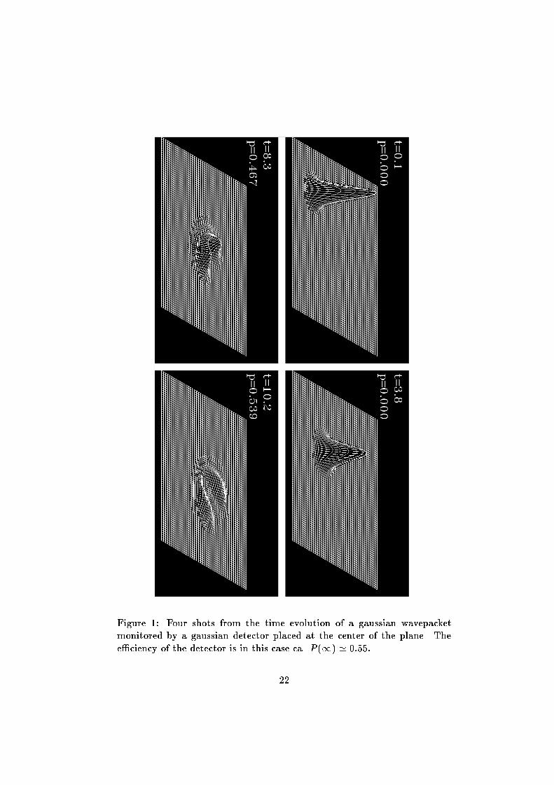
Figure 1: Four shots from the time evolution of a gaussian wavepacket

monitored by a gaussian detector placed at the center of the plane. The

e�ciency of the detector is in this case ca. P (1) ' 0:55:

22

0.0 0.5 1.0 1.5 2.0 2.5 3.00.0

0.5

1.0

Probability density p(t)

alpha=4.0

alpha=16.0

alpha=2.0

alpha=1.0

alpha=0.01

alpha=100.0

Figure 2: Probability density of time of arrival for a Dirac's delta counter

placed at x = 0, coupling constant alpha. The incoming wave packet starts

at t = 0, x = �4, with velocity v = 4

0.0 1.0 2.00.000

0.500

1.000

1.500

2.000

2.500

Rescaled probability density p(t)

Figure 3: Rescaled probability densities of Fig.1

23

0.0 1.0 2.0 3.0 4.0wave packet velocity v

0.0

1.0

2.0

3.0

4.0

5.0

6.0

7.0

8.0

coup

ling

cons

tant

alp

ha

Optimal coupling constant

Figure 4: Optimal coupling constant as a function of velocity of the incoming

wave packet. The dependence pretty soon saturates to a linear one. At the

saturation value P (1) � 0:5:

0.0 1.0 2.0 3.0 4.0 5.0 6.0 7.0 8.0 9.0 10.0coupling constant alpha

0.0

0.1

0.2

0.3

0.4

0.5

0.6

0.7

0.8

P(in

finity

)

Static wave packet over the counter

Figure 5: P (1) as a function of � for a static wave packet centered over the

counter. The maximum, of P (1) = 0:725448 is reached for � = 1:3216:

24

0

1

2

3

4

5

v

0

2

4

6

8

alpha

0

0.1

0.2

0.3

0.4

0.5

0.6

0.7

P(inf)

Figure 6: P (1) as a function of velocity v and coupling constant � for a

static wave packet centered over the detector.

25