Time horizon trading and the idiosyncratic risk puzzle

Electronic copy available at: http://ssrn.com/abstract=1891985

TIME HORIZON TRADING AND THE IDIOSYNCRATIC RISK PUZZLE∗

JULIANA MALAGON, DAVID MORENO and ROSA RODRÍGUEZ

University Carlos III- Department of Business Administration

JEL-classification: G12

November, 2011

∗ We are grateful for helpful comments and suggestions on Wavelets Multiresolution Analysis by Agnieska Jack. David Moreno ([email protected]) acknowledges financial support from Ministerio de Ciencia y Tecnología grant ECO2010-17158. Rosa Rodríguez ([email protected]) acknowledges financial support from Ministerio de Ciencia y Tecnología grant ECO2009-10796. Corresponding autor: Juliana Malagón ([email protected]) acknowledges financial support from Comunidad de Madrid grant CCG10-UC3M/HUM-5237. University Carlos III. Department of Business Administration. C/ Madrid, 126, 28903- Getafe – Madrid –Spain.

Electronic copy available at: http://ssrn.com/abstract=1891985

2

Time Horizon Trading and the Idiosyncratic Risk Puzzle

ABSTRACT

We analyze if the idiosyncratic risk puzzle pointed out by Ang et al., (2006, 2009) can be explained by the existence of market participants with different investment horizons. We adopt a Wavelet Multiresolution Analysis to decompose returns distribution in different time-scales. Our approach splits the nonlinear link between expected returns and idiosyncratic risk into two linear relationships: a positive one for long run investors and a negative one for short run agents indicating that the puzzle disappears as the wavelet scale increases (log-term horizons). Our results are robust to several types of wavelets, different definitions of short-term investors and to various measures of idiosyncratic risk.

JEL-classification: G12

Keywords: idiosyncratic risk, wavelets, time-scaling risk

Electronic copy available at: http://ssrn.com/abstract=1891985

3

1. Introduction

The relationship between idiosyncratic volatility and expected returns has become a

major issue in recent research. 1

Maybe because of its controversial nature literature was reactionary to the idiosyncratic

volatility – expected returns puzzle, this is, the concept of idiosyncratic risk’s pricing

ability. Thus, after the publication of the paper most of the literature focused on showing

that the puzzle was somehow mistaken and discussed the robustness of Ang et al., (2006)

results. For example, Bali and Cakici (2008) argued that the negative relationship either

disappears or is not significant depending on data frequency, on the weighting scheme used

to calculate average portfolio returns, on breakpoints used to sort portfolios’ quintiles and

on the inclusion of small illiquid stocks in the sample. A similar result was obtained by Fu

(2009) who argued that Ang et al., (2006) mistakenly conclude the link between

idiosyncratic risk and expected returns is negative because they assumed that idiosyncratic

volatility is persistent. Using an EGARCH model to take into account heterocedasticity in

idiosyncratic volatility he finds a positive and significant result.

The current debate surrounds the evidence shown by Ang

et al., (2006) who, creating quintile portfolios sorted by stocks based on idiosyncratic risk

levels, found that the portfolio with the highest level of idiosyncratic risk has significantly

lower returns than the one with the lowest level. This negative liaison is indeed a

controversial idea since it challenges both modern portfolio theory and under-

diversification models (Merton, 1987). The former virtually assumes no link at all and the

later assume a positive link driven by lack of investors’ diversification capacity.

After the initial criticisms, Ang et al., (2009) proved the robutness of their puzzle

basically by examining not only American data but also data from all other countries from

the G7 (Canada, France, Italy, Germany, Japan, U.S and UK). Again, they found the same

negative and significant relation between idiosyncratic volatility and expected returns for

all countries. Furthemore, the American data results were shown to be robust to different

1 Even if the recent debate has put the discussion on returns’ predictability using idiosyncratic risk back on the picture, the issue has long been discussed in the past. Both Douglas (1969) and Lintner (1965) find a significant explanatory power of the variance of the residuals from a market model in the cross-section of average stocks returns. Later Miller and Scholes (1972) and Fama-Macbeth (1973) argue some statistical problems. And finally Lehmann (1990) reaffirms Douglas’ results after a careful econometrical revision.

4

weighthing portfolios’ formation and also to the use of different periods to compute

idyosincratic risk. This second paper marked a breaking point in literature. Indeed, after its

publication the puzzle gained credibility so that lately the discussion has turn to find

possible answers to the question of why the relationship is found. Our paper is part of this

literature trying to provide new insights to this puzzle.

One of the relatively recent hypotheses is that the so called volatility - returns puzzle is

driven by investors heterogeneity in the financial markets. In this sense, Brandt et al.,

(2008) argue that the puzzle is driven by retail investors, which have a special preference

for stocks with high idiosyncratic volatility, compared with institutional investors, which

tend to minimize their exposure to this type of assets. However, some authors argue

mutuals funds’ managers have a preference for stocks with high idiosyncratic risk

(Falkenstein, 1996) and that, when willing to increase their risk they increment their

portfolio exposure to idiosyncratic one (Huang et al., 2011). In this paper we assume the

perspective of heterogeneity of market players focusing specifically on heterogeneity in

investors’ time horizons. Financial markets are comprised of investors and traders with

different investment time horizons: market makers, intraday investors, day investors, short-

term traders and finally long-term traders. The aggregation of the activities of all them is

what ultimately generates prices. The implication of the heterogeneity assumption is that

the true dynamic relationship between the various aspects of market activity will only be

revealed when the market prices are decomposed by the different time scales or different

investment horizons.

Both heterogeneity of investors and time horizons are by themselves important concepts

for asset pricing. On the one side, financial empirical stylized facts such as fat tails and

volatility clusters are difficult to explain in the context of homogeneous investors while

they naturally arise in computational markets with different types of investors (Lévy et al.,

2000, Gil-Bazo et al., 2007). On the other side, empirical tests of risk loadings depend

largerly on time interval and systematic risk is biased when using a shorter investor’s time

horizon than the true one (e.g. Levhari and Levy, 1977). By extension, considering

heterogeneous investors in the sense of differences in time horizons should impact

5

idiosyncratic volatility estimation and thus can be expected to enhace the study of the

puzzle we are interested in. However, this approach entails the problematic issue of

separating investors classes and their influence on idiosyncratic volatility and returns.

Wavelet Multiresolution Analysis (WMRA) is very useful to tackle time horizons

differentiation problem. It allows the decomposition of a time series into different time

horizons, called time scales, each corresponding to a particular frequency. Since different

investors have different trading frequencies, the first scale should yield information on

short-term investors while the higher scale should provide information about long-term

investors (Müller et al., 1997, Gençay et al., 2005 and 2010 and In and Kim 2006 and

2009). In this context asset pricing models could yield different results on each time scale,

as it is in fact the case (Gençay et al., 2003, 2005), and the negative risk-return link shown

by Ang et al., (2006, 2009) might not be valid for all investors.2

Alternative explanations state the puzzle is observed given that stocks with the highest

levels of idiosyncratic risk are difficult to short-sale so that pessimistic information does

not flow to these stock prices (Boehme et al., 2004, Asquith et al., 2005). An additional

proposal by Boyer et al., (2010) argues stocks with higher idiosyncratic risk offer larger

probabilities of an extreme positive return and thus have lower returns. Finally, in Berrada

and Hugonnier (2010) the puzzle is related to firms’ cash flow growth rate. While these authors

suggest that explanations for the observation of the puzzle are related to the specific

characteristics of the stocks or the firms with the highest level of idiosyncratic risk, we

argue investors’ characteristics are also relevant.

The main goal of this paper is to separate short-term investors and long-term investors

through a WMRA, using daily data to study separately their influence in monthly stock

prices. We can therefore, analyze the puzzle for each group separately. This approach has

2 Wavelet analysis is relatively new in economics and finance, although the literature on wavelets is growing rapidly. Applications in these fields include the study of systematic risk in the capital asset pricing model (Gençay et al. 2003 and N. Rhaiem et al., 2007), the multi-scale relationship between stock returns and inflation (Kim and In, 2005), the relation between returns and systematic co-kurtosis and co-skewness (Galagedera and Maharaja, 2008), a multiscale hedge ratio (In and Kim 2000), studies in portfolio management (In et al. 2008 and Bowdena and Zhub, 2010) portfolio allocation (In and Kim 2010), the analysis of co-movements in stock markets (Rua and Nunes, 2009), Value at Risk measures ( Fernandez, 2005) and credit portfolio losses (Masdemont and Ortiz-Gracia, 2009).

6

not, to the best of our knowledge, been applied before to the idiosyncratic volatility –

expected returns puzzle. We conjecture the negative relationship is driven by short-term

investors who do not necessarily follow the typical mean-variance logic for which Ang et

al., (2006, 2009) result is puzzling. Our results confim that the puzzle disappears as the

wavelet scale increases; idiosincratic risk – returns relationship turns positive at larger

scales indicating that investors with long run horizons should not worry about the puzzle as

compared to those with short-term horizons. Moreover, our approach provides an

explanation covering all the stocks (not only the riskiest ones) and are robust to changes in

wavelet family, idiosyncratic risk estimators and co-skewness or liquidity factors.

The remainder of the paper is organized as follows. Section 2 gives a general discussion

of empirical asset pricing models tests that justifies the use of wavelets decomposition for

this particular analysis. Preliminary evidence of the puzzle in our sample is given in section

3. Section 4 describes the Wavelets and Multiresolution Analysis methodology and the

empirical results. Section 6 analyzes the robustness of our findings and Section 7

concludes.

2. Empirical tests of asset pricing models, time horizons and wavelets

Given the continuous nature of price formation it is mainly impossible to determine the

correct time interval to empirically test asset pricing models. This is one of the reasons why

basically any empirical study is subject to critiques on data frequency such as the ones

made to Ang et al., (2006, 2009) by Bali and Caciki (2008), who show that using monthly

instead of daily data achieves different conclusions about the idiosyncratic risk – expected

returns relationship. Nevertheless, it is well known that systematic risk depends largely on

the interval over which returns are measured (Levhari and Levy, 1977, Hawawini, 1983,

Handa et al., 1993, Brailsford and Josev, 1997, Brailsford and Faff, 1997, among others) 3

3 In particular beta of thinly traded securities increases as the return interval rises while the one of frequently traded securities falls. Also the estimated beta of high capitalized firms decreases as the return interval increases while the beta of low cap firms increases.

.

Also, the so-called Epps effect (Epps, 1979) shows that stock return correlations decrease

as return interval increases. As risk measures change with return interval (i.e. implied

7

investor time horizon), the idiosyncratic risk estimation is also expected to change

introducing the necessity of studying the puzzle for different time horizons.

From a statistical point of view, a possible reason for the mixed evidence on empirical

tests of asset pricing models might be the divergence between theoretical assumptions used

in models’ construction and the empirical evidence itself. In an efficient market, asset

prices reflect all relevant and available information and any news affecting them is

simultaneously and immediately incorporated into prices. New information has to be

independent and random in order not to be anticipated and immediately translated to prices.

Thus, the instanteneous adjusment implies independence of price increments and a sigular

time horizon. However, stylized facts such as volatility clustering and fat tails contradict

this i.i.d assumption. In this context, Heterogeneous Agents Models state that the market is

formed by investors with different characteristics who judge which information is relevant

according to their nature.4 We specifically consider the case of market participants with

different time horizons. Under this perspective, information is diffused unevenly,

independence of price increments does not hold and asset prices reflect a combination of

long and short-term valuation processes. 5

So far, we have introduced three concepts namely, time-horizons, frequency and scale.

As shown before, time-horizons determine frequencies. On the other hand, scale and

frequency are directly related so that time-scaling risk corresponds to the notion of risk

being differently assessed by investors with various time-horizons. Differing investment

horizons violate the independence assumptions and thus introduce global (in opposition to

serial) dependences on the return series. These are very difficult to assess with ARMA or

In this case, financial risk depends not only on

time but also on the particular investment horizon; financial risk is both time-varying and

time-scaling (Los, 2003).

4 Heterogeneous Agents Models (Müller et al., 1993, 1997, LeBaron, 2000) are theoretical explanations for empirical stylized facts based on the existence of differences in investors. Müller argues that differences can be observed in perceptions, institutional constraints, risk profiles, prior beliefs or geographical location. We focus on the idea of differences in time horizons since it offers the possibility of the mathematical treatment we show herein. 5 O’Hara (2003) discusses the impact of diverging information within the classical asset pricing models assumptions. Her main conclusion is that asymmetric information derives into a group of uninformed (noise) traders that, even if they systematically lose to better-informed ones, make portfolio choices so that their risk exposure to wins of informed investors is lower.

8

GARCH family models since correlations are only transient or have varying frequencies. In

turn, to analyze risk in this framework it is necessary to change the analytical tools used in

most of finance literature to allow for different time-scales. A major recent development

dealing with the time-scales issue in financial data is Multiresolution Analysis from

Wavelet decomposition (Mallat, 1989) appeared in the late 1980s. Next section summarizes

the main features of this statistical tool that provides an additive decomposition in which,

instead of differentiating a trend, a seasonal and a cyclic component, a time series is viewed

as a sum of time-scales each of them able to account for local changes.

2.1.Wavelets methodology and Multiresolution Analysis

Considering global (long-term) dependence in market returns is to say that returns

series are non-stationary and that financial risk’s assessment involves more than the first

two moments of the distribution (Mandelbrot, 1972). In order to obtain evidence for any

form of time dependence it is necessary to have both the distributional and the time-

localized evidence at the same time.

The first technique known to build information on frequencies for a given time series

was Fourier analysis. Fourier transform is not suitable for financial data since it is only

meaningful when the time series is stationary and does not have sudden changes. Also, the

transform loses all time-dependence information so that global dependences are impossible

to isolate using this technique.

Wavelet transform is similar to Fourier transform but does not lose time information

because wavelets are localized both in time and frequency. In addition, wavelets are

functions with finite time support so that they are able to cope with sudden changes in

signals. We are interested in a particular feature of Wavelet Analysis: The Wavelet

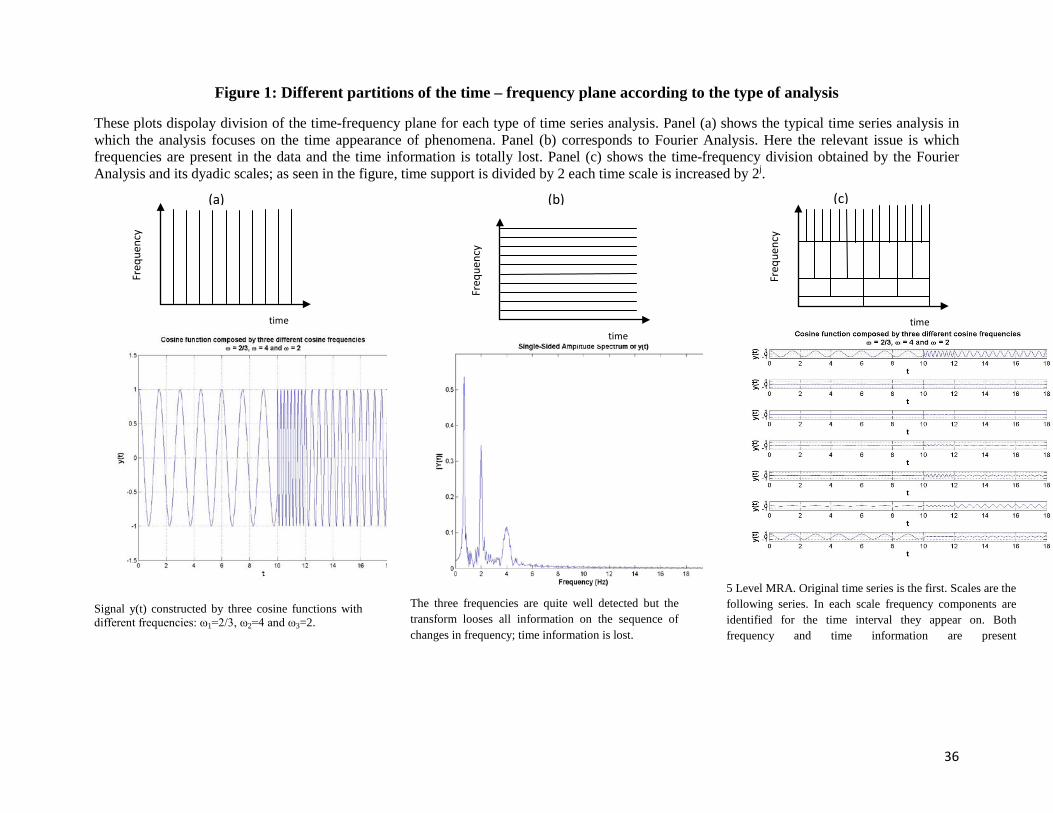
Multiresolution Analysis (WMRA). This technique divides the time-frequency space into

frequency bands separated by multiples of 2j and which time support is divided by 2 as

frequency increases. In Figure 1, we can observe the division of the time-frequency plane

for each type of time series analysis followed by a plotted example using a cosine function.

Panel (a) shows the typical time series analysis which focuses on the time appearance of

9

phenomena; the plot considered here corresponds to a signal constructed using three cosine

functions with frequencies 2/3, 4 and 2. Panel (b) corresponds to Fourier analysis. Here the

relevant issue is which frequencies are present in the data and the time information is

totally lost. Therefore the plot shown only provides information on frequencies. The three

frequencies are detected but time information is lost; it is impossible to know when a

change of frequency appeared or the order of their appearance. Panel (c) shows the time-

frequency division obtained by the Fourier analysis and its dyadic scales; as seen in the

figure, time support is divided by 2 each time scale is increased by 2j. The plot displays a 5-

level WMRA in which both time and frequency information are present; in each time scale,

frequency components are identified for the time interval they appear on.

[Figure 1]

Performing a WMRA, a time series S0 is decomposed into a blurred approximation Si

(long run horizon) and the remaining details Di (short run horizons), where Si and Di are

orthogonal from each other. The resulting series in the time domain are the contribution of

frequency i to the original series or the component of the original series that has frequency j

(Norsworthy et al., 2000).

Mallat (1989) developed a method to perform the WMRA of a signal through simple

linear filters that separate its high frequency elements (corresponding to the details) from its

low frequency ones (corresponding to the blurred approximation). Frequency separation is

done using two linear filters, each blocking a particular frequency (high or low) while

letting the other (low or high) pass through. The series are recomposed into the time

domain using the corresponding quadrature mirror filters. There are many Wavelet

Transform classes and Wavelets families with particular properties. We use the Maximum

Overlapped Discrete Wavelet Transform (MODWT) and the Haar Wavelet Family (Haar,

1910) for which filter coefficients are 𝐻0 = � 1√2

, 1√2� for the low pass filter and 𝐺0 =

�− 1√2

, 1√2� for the high pass filter. Both the scale series and the details series are obtained

using the quadrature mirror filters 𝐻0���� = � 1√2

, 1√2� and 𝐺0���� = � 1

√2,− 1

√2�.

10

3. Data Description and Preliminary Evidence

In this section we follow Ang et al., (2006) procedure to confirm the idiosyncratic

volatility – expected returns puzzle for our sample before addressing any time horizon issue

using wavelets. Our database includes daily returns of all stocks in the CRSP (Chicago

Research Stock Prices) with more than 17 observations in a month for NYSE, AMEX and

NASDAQ markets from July 1963 to December 2009. For each month, we sort stocks

according to their idiosyncratic volatility, defined as the standard deviation of the residuals

in the Fama and French (1993) three factor model (σεti ),

rti = αi + βMKTi MKTt + βSMBi SMBt + βHMLi HMLt + εti , [5]

where, rti is the stock returns in excess of the risk free rate and {𝑀𝐾𝑇𝑡, 𝑆𝑀𝐵𝑡,𝐻𝑀𝐿𝑡}

represent the market, size and book to market factors.6 Once we have sorted the stocks into

quintiles, where the first one contains stocks with the lowest risk and the last one those with

the highest risk, we form portfolios and hold them for one month. The corresponding

portfolios are value-weighted and rebalanced month by month.7

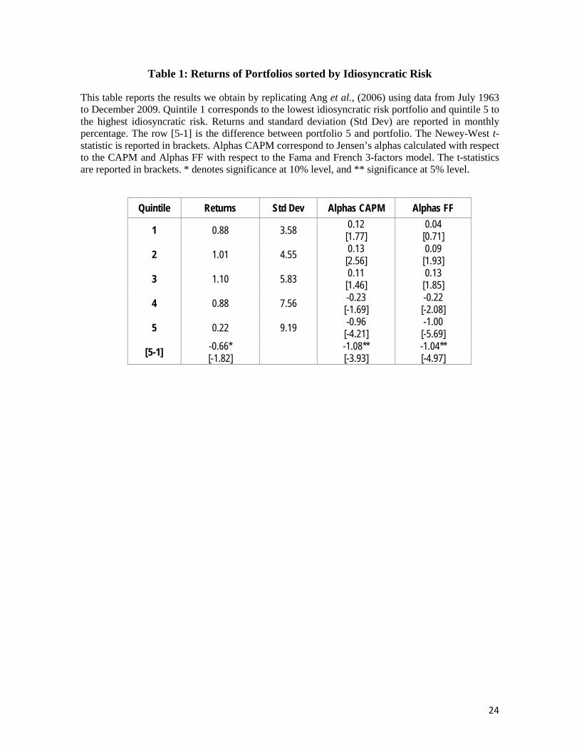
Table 1 reports the results obtained by replicating Ang et al (2006) process using data

from July 1963 to December 2009. In columns we present the average returns, standard

deviation, and alphas for portfolios sorted on idiosyncratic volatility. All of them are

reported in monthly percentage. Alphas CAPM correspond to Jensen’s alphas calculated

with respect to the CAPM and Alphas FF with respect to the Fama and French three-factor

model. The t-statistics are reported in brackets. The row [5-1] is the difference between

portfolio 5 and portfolio 1 where Newey-West t-statistic is also reported in brackets.

[Table 1]

Main patterns reported by Ang et al., (2006) appear on our sample. Average returns of

portfolios sorted on idiosyncratic volatility display an inverse U-shaped form increasing in

the middle quintiles; returns rise from 0.88% in quintile 1 to 1.10% in quintile 3, then drop

6 They have been obtained from Kenneth French’s website http://mba.tuck.dartmouth.edu/pages/faculty/ken.french/data_library.html 7 We also verify the puzzle using 6 months for the regression in equation [5] in order to address the critique of error-in-variance exposed by Malkiel and Xu (2002). Results don’t change. They are available upon request.

11

to 0.22% in quintile 5. The difference [5-1] is in average -0.66% per month. It is negatively

significant at 10% when using Newey-West t-statistic and at 5% when using White

Heteroskedasticity-Consistent t-statistic. Moreover, Jensen’s alphas are positive for the

initial three portfolios and change sign to negative from the fourth. Both [5-1] differences

in CAPM alphas and in FF alphas are negative, -1.08% the former and -1.04% the latter,

showing the puzzle appears even after controlling for risk. Having similar patterns in our

results provides evidence of the robustness of Ang et al., (2006, 2009)’s results; their main

conclusions hold for a longer period and are not modified by the particularly unstable times

characterizing the lately years of our sample.

Since asset pricing models impact idiosyncratic volatility estimation, a remaining

question is if the puzzle is robust to different models. We replace the Fama and French

three-factor model by the Carhart (1997) model so that the idiosyncratic volatility used to

sort the stocks is the standard deviation of the residuals from the following equation:

𝑟𝑡𝑖 = 𝛼𝑖 + 𝛽𝑀𝐾𝑇𝑖 𝑀𝐾𝑇𝑡 + 𝛽𝑆𝑀𝐵𝑖 𝑆𝑀𝐵𝑡 + 𝛽𝐻𝑀𝐿𝑖 𝐻𝑀𝐿𝑡 + 𝛽𝑀𝑂𝑀𝑖 𝑀𝑂𝑀𝑡 + 𝜀𝑡𝑖, [6]

where, 𝑟𝑡𝑖 is the stock excess returns and {𝑀𝐾𝑇𝑡, 𝑆𝑀𝐵𝑡,𝐻𝑀𝐿𝑡,𝑀𝑂𝑀𝑡} represents the

market , size, book to market and momentum factors.

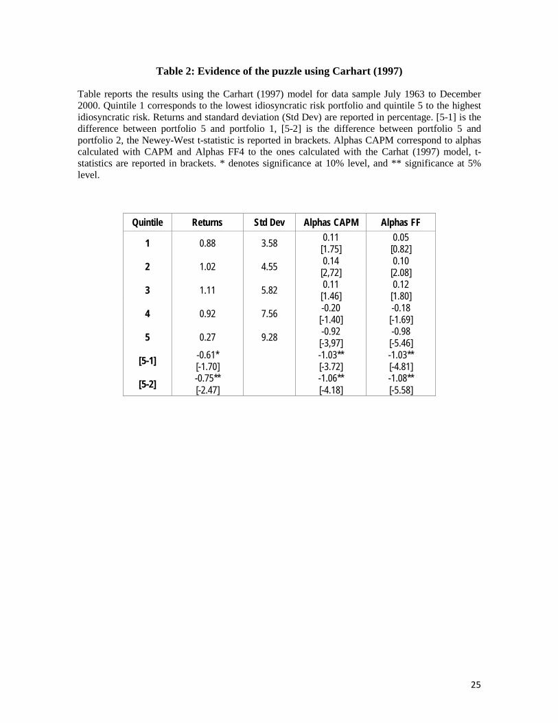
Table 2 illustrates the results under Carhart’s model. As in the previous table, returns

and standard deviations are monthly averages in percentages and alphas for CAPM and

Carhart’s model are tabulated. All t-statistics are in brackets.

[Table 2]

Qualitatively results in alphas, returns and standard deviations are similar and the [5-1]

returns difference is equal to -0.61% but only significant at the 10% level. However, the

puzzle can be verified using the second quintile portfolio since the fact that a riskier

portfolio yields lower returns also appears for the fifth and second quintiles. The negative

link is significant at the 5% level if one considers the [5-2] returns difference.8

8 Although not reported here, the significance of the [5-1] difference is sensitive to the time period considered. Only for three months in the sample ending in months from November 1990 to December 2009 the difference is not significant either at 5% or at 10% levels. These results are available upon request.

Therefore,

12

controlling for momentum is not relevant to explain the puzzle.9

At this point we have

proven the puzzle is present in our sample together with its robustness to changes in

idiosyncratic risk estimation. We can now turn to time horizons implications on

idiosyncratic risk – expected returns relationship.

4. Methodology and Empirical results

In this section we briefly describe the process followed for the wavelet approach to

shed some light into the expected return – idiosyncratic risk puzzle. We distinguish several

time-scales, each corresponding to a group of investors with a particular and homogeneous

time horizon. Our hypothesis is that investors value information according to their

investment horizon so that for each group a different idiosyncratic risk – expected return

link might be observed.

Theoretically, once the Efficient Market Hypothesis is dropped by introducing

differing time-horizons, the number of investors groups to be taken into account is not

limited. Neither is this number limited by the WMRA nature. Therefore, the first stage of

the analysis is to decide the number of time-scales to be considered. Many articles

including portfolio rebalancing limit the number of time-scales to the maximum possible

number before the rebalancing (Gençay et al., 2003, 2005). With daily data, an one level-

MRA divides the data into two investment horizons (2 to 4 days and more than 4), a two

level-MRA divides the data into three investment horizons (2 to 4 days, 4 to 8 days and

more than 8), a three level-MRA divides the data into four investment horizons (2 to 4

days, 4 to 8 days, 8 to 16 days and more than 16).10

For each level-MRA and time-scale we calculate the Fama and French 3-Factor model

and sort the stocks according to the standard deviation of the residuals. Then, we compute

the five portfolio quintiles and focus our attention on the difference in the returns from the

Then, the maximum number of time-

scales is three since our rebalancing is done monthly (i.e. approximately 17 to 20 days).

9 The same conclusion was already found by by Ang et al., (2006) through another methodology. They included a double sorting control for momentum after which the puzzle still yields. 10 Notice that, as said before, time-scale increases by multiples of 2j and we are working with daily data. Therefore time-scale increases in 2j days each time; 2-4 days, 4-8 days, 8-16 days and so on.

13

fifth to the first quintile. This procedure produces two time-scales (D1 and S1) for the one

level-MRA, three time-scales (D1, D2 and S2) for the two level-MRA and, four time-scales

(D1, D2, D3 and S3) for the three level-MRA. Since WMRA is performed recursively, both

D1 and D2 time-scales are the same for any level-MRA.

It can be expected to isolate short-term investors’ (e.g. technical analysts) behavior on

the finer scale of the MRA.11

We begin by the simplest case in which there are only two groups of investment

horizons, short-term (2 to 4 days) and long-term (more than 4 days), corresponding to D1

and S1 respectively. The decomposition linked to this hypothesis is the one level – MRA

for which results are reported in Table 3. The structure of this table is analogous to the

initial tables but duplicates columns in order to display information for both investors’

groups. The first four columns correspond to the analysis for short-term investors (D1).

Returns and standard deviations are average monthly percentages across portfolios and last

two columns for each group display CAPM and FF alphas. The last four columns illustrate

the results for long-term investors. All t-statistic values are tabulated in brackets.

By extension, fundamentalists’ behavior should be reflected

at a coarser scale. Because idiosyncratic risk - expected returns puzzle can’t be explained

by classical portfolio theory, financial data empirical characteristics provide evidence

supporting the hypothesis of multiple types of investors in the market, and long-term

investors are expected to follow fundamentals (i.e. they are close to the representative agent

in classical asset pricing models). This is consistent with the findings of Gençay et al.

(2005) that the relationship between the return of a portfolio and the systematic risk

measure becomes stronger as the investment horizon increases. Then, we expect the

negative idiosyncratic volatility – expected returns liaisons disappear at coarser scale.

[Table 3]

Results back up our hypothesis in that the puzzle is only present for short-term

investors. For this group (D1) the [5-1] returns difference is significantly negative and

11 It has been shown that technical analysis is mostly used for short-term forecasting (Frankel and Froot, 1990). However, we prefer to let the exact nature of investors an open issue and limit our classification to the relative frequency of trading of each group of investors considered in the MRA. This is because we consider that investors use all tools available for decision making no matter how frequently they trade.

14

equal to -0.96%. Also, the puzzle remains after controlling for CAPM and FF risk factors;

[5-1] differences in both models’ alphas are negative; -0.009 and -0.004 respectively. For

long-term investors (S1) the puzzle disappears and the [5-1] difference takes a positive and

significant value of 0.90%.

A noteworthy result is that average monthly returns sorted by idiosyncratic risk do not

longer exhibit an inverse U-shaped form. For short-term horizons, returns decrease linearly

from -0.09% in the first quintile to -1.04% in the last one. In the case of long-term horizons,

returns increase from 1.01% for the portfolio with the lowest idiosyncratic risk to 1.91% for

the riskiest one. These patterns support the idea of an asset price formation resulting from

two heterogeneous groups. In this sense, the inverse U-shaped pattern in returns indicates a

nonlinear relationship between idiosyncratic risk and expected returns that we argue to be

caused by the interaction of investors with dissimilar time horizons. Alternatively, returns’

U-shaped form could be the result of a missing risk factor. However, we think our results

back up our working hypothesis in the fact that a non-linear liaison related to a missing risk

factor should be reflected for both short and long-term investors. In addition, our results are

corroborated by a recent study by Cao and Xu (2010) who decomposing the idiosyncratic

volatility into long-run and short-rum components find the existence of a negative short-run

effect.

Another significant but challenging fact is that for short-term horizons all portfolios

have negative returns (-0.09%, -0.15%, -0.26%, -0.47% and -1.04%). We conjecture that

the highest frequency scale is isolating short-term strategies which objectives differ from

the typical mean-variance strategy and that the negative results are random. Alternative

explanations can be provided by O’Hara’s idea of a group of investors (uninformed)

persistently losing to the other group (informed) while rationally minimizing their risk

exposure (O’Hara, 2003) or by Fractal Hypothesis Market in which the negative signs can

be understood as evidence of the higher likeliness of crowd behavior in short-term

movements.12

12 Adopting O’Hara’s idea would require identifying short-term investors with uninformed ones. However our evidence is not enough to do it. Fractal Market Hypothesis proposes that information is more related to

15

On the other hand, before the decomposition into time horizons the negative link

between expected returns and idiosyncratic risk is driven by a notorious drop of -75% (this

is 0.22 - 0.88) in returns from the fourth to the fifth quintile. In this sense Brandt et al.,

(2008) and Han and Kumar (2009) report the negative idiosyncratic volatility – expected

returns tie is stronger for small low priced stocks typically hold by retail investors.13

However, in our analysis retail investors might perfectly be in any of the two categories of

investors, most likely they are represented in both groups, and for short-term investors the

notorious drop in the last quintile portfolio return remains. Other explanations of the puzzle

relate this notorious drop to the type of stocks classified in the fifth quintile (e.g. Asquith et

al., 2005, Boehme et al., 2006). Given that in the case of short-term investors changes from

quintile to quintile are similar (increases of 100% approximately), showing the linear

relationship described earlier, the idea that the puzzle is determined by stocks with special

features being classified into the fifth quintile is not supported. These stocks are represented

both in the short-term series (Di) and in the long term ones (Si) so that if they were driving

the puzzle it should be observed in both groups. Even if these stocks might be related to the

puzzle because of some special feature they offer, only the movements of short-term

investors explain the appearance of a negative relationship between idiosyncratic risk and

returns.

5. Robustness

In this section we study if our main result (that the puzzle is present in the short

horizon but not in long horizons) is robust to several estimators of idiosyncratic risk, and

different definitions of short-term investors.

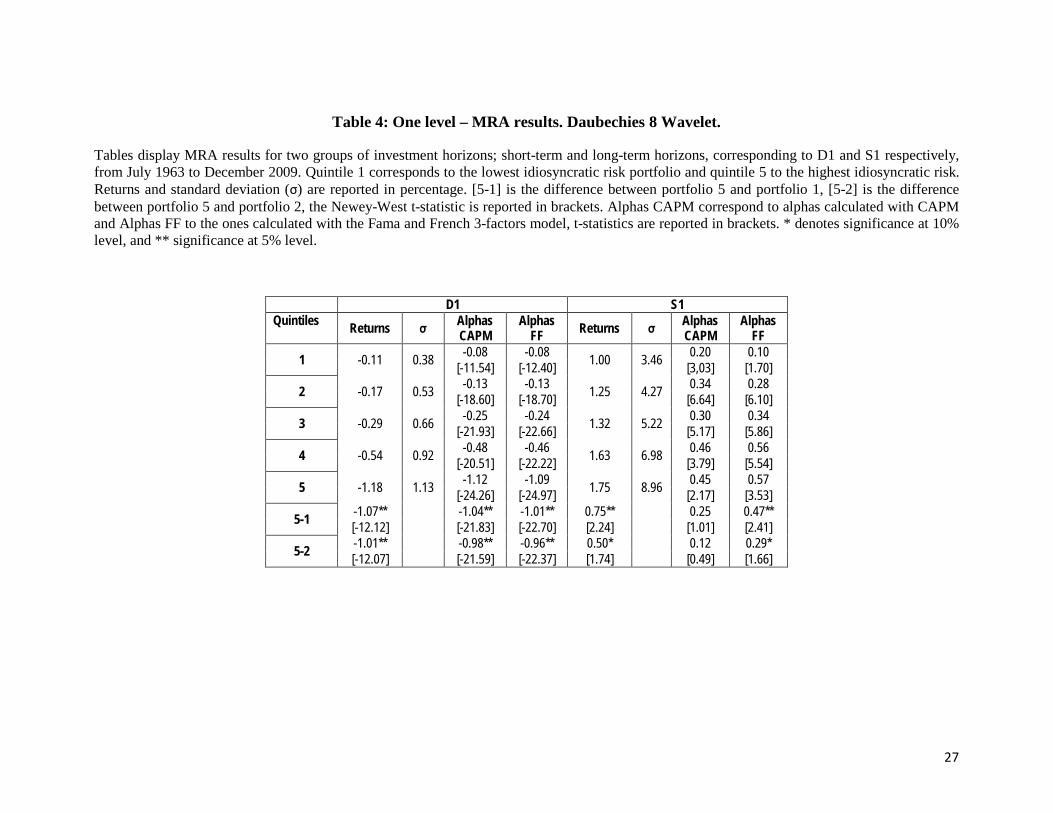
Wavelet family might have an influence on the results since it imposes the length of

the MRA filter. A longer filter implies a larger adaptability to complex time series in the

WMRA. In Table 4 we display the one level MRA for two groups of investors, short-term

market sentiment and technical factors in the short-term than in the long term, and that short-term price movements are likely to be the result of crowd behavior (Blackledge, 2010). 13 Authors argue retail investors are especially interested in these stocks because of their speculative character: high skewness and high volatility.

16

and long term investors, corresponding to D1 and S1 respectively, for a Daubechies 8

wavelet.14

[Table 4]

Figures reported on Table 4 show a [5-1] returns’ difference significant and

negative for short-term investors (-1.07%) but significant and positive (0.75%) for long-

term ones. Also, for both groups, idiosyncratic risk and returns are linearly related; returns

monotonically decrease from -0.11% to -1.18% for D1 and monotonically increase from

1.00% to 1.75% for S1. Consistency of results across different wavelet families leads us to

the conclusion that wavelet family is not driving our conclusions.

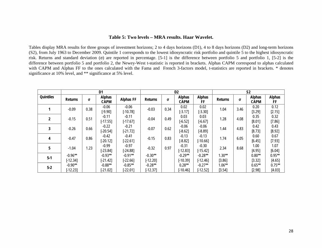
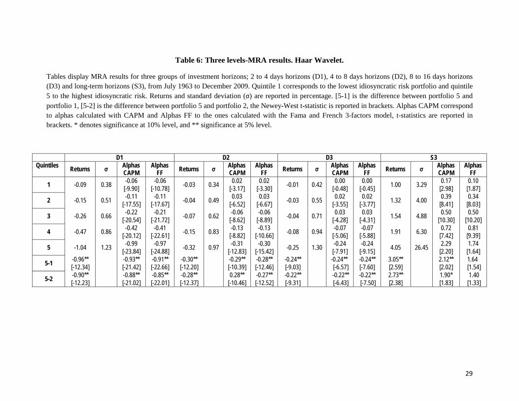
In Tables 5 and 6 we present a two-level and a three-level MRA respectively in

order to include more investors groups. As explained in section 4, D1 represents the 2 to 4 days

investors. D2 the 4 to 8 days investors, D3 the 8 to 16 days investors and S2 and S3 represent

long-term investors. The tables follow the same structure of the previous ones but include

additional columns with the information for D2, D3, S2 and S3 accordingly with the MRA-

level considered.

For alternative definitions of short-run the puzzle remains; risk and returns are

significantly and negatively related both for D2 (-0.30%) and D3 (-0.24%). In these cases

portfolios’ returns are also negative for all short-term horizons definitions. However, both

the magnitude of the negative relationship constituting the puzzle and its significance level

diminishes as investment horizon increases.

[Tables 5 and 6]

In addition, we build a monthly S1 series for stocks with no missing values over the

sample period and determine short-term investors influence by comparing it to the monthly

original series. We find that, even if in the daily decomposition short-term movements are

relevant, compounding the daily long-term series (S1) produces basically the same series

than the original. In fact, over the whole period only 21% of the stocks have points outside 14 Although many other possibilities exist, in this paper we consider only the Haar and the Daubechies wavelet families. We consider the Haar family as our benchmark because many of the previous literature available on risk loadings in asset pricing models use it. Keeping the same family allow comparisons. Daubechies family is a natural extension in that Haar wavelets is the Daubechies wavelet of minimum length. It is also a common wavelet family when it comes to studies in economics and finance. See for example Yanqin and Gençay (2010) or Huang and Wu (2008)

17

the one standard deviation interval. From these, 73% have only one point and 100% have 4

or less points outside it. Monthly S1 and the original series are very similar in terms of

mean and standard deviation and have very large correlations (0.99 in mean) but there are

marked differences in terms of skewness and kurtosis for some of the stocks.15

In order to discard this alternative explanation we introduce a coskewness factor into

the asset pricing model used to estimate idiosyncratic volatility. Using all stocks with more

than 220 daily observations available, we calculate a daily coskewness factor. For each

stock and year we calculate the Harvey and Siddique (2000) coskewness measure,

Then, it is

possible that stocks in the highest quintile are stocks with higher coskewness values so that

the lower returns in the last quintile are explained by stocks offering a larger probability of

extreme values.

𝐶𝑜𝑠𝑘𝑖 = 𝐸�𝜀𝑖,𝑡+1𝜀𝑀,𝑡+12 �

�𝐸�𝜀𝑖,𝑡+12 �𝐸�𝜀𝑀,𝑡+1

2 �, [7]

where, for each stock 𝜀𝑖,𝑡+1 are the residuals from the regression of the excess return on the

contemporaneous market excess return and 𝜀𝑀,𝑡+1 are the residuals of the excess market return over

its mean.

Then we sort stocks into three portfolios, cutting at 30% and 70%, and consider the

two extreme ones. Factor’s value weighted returns are calculated for the next day as the

difference between the return on the lowest coskewness portfolio and the highest

coskewness portfolio. The procedure is repeated by rolling the initial window by one day.

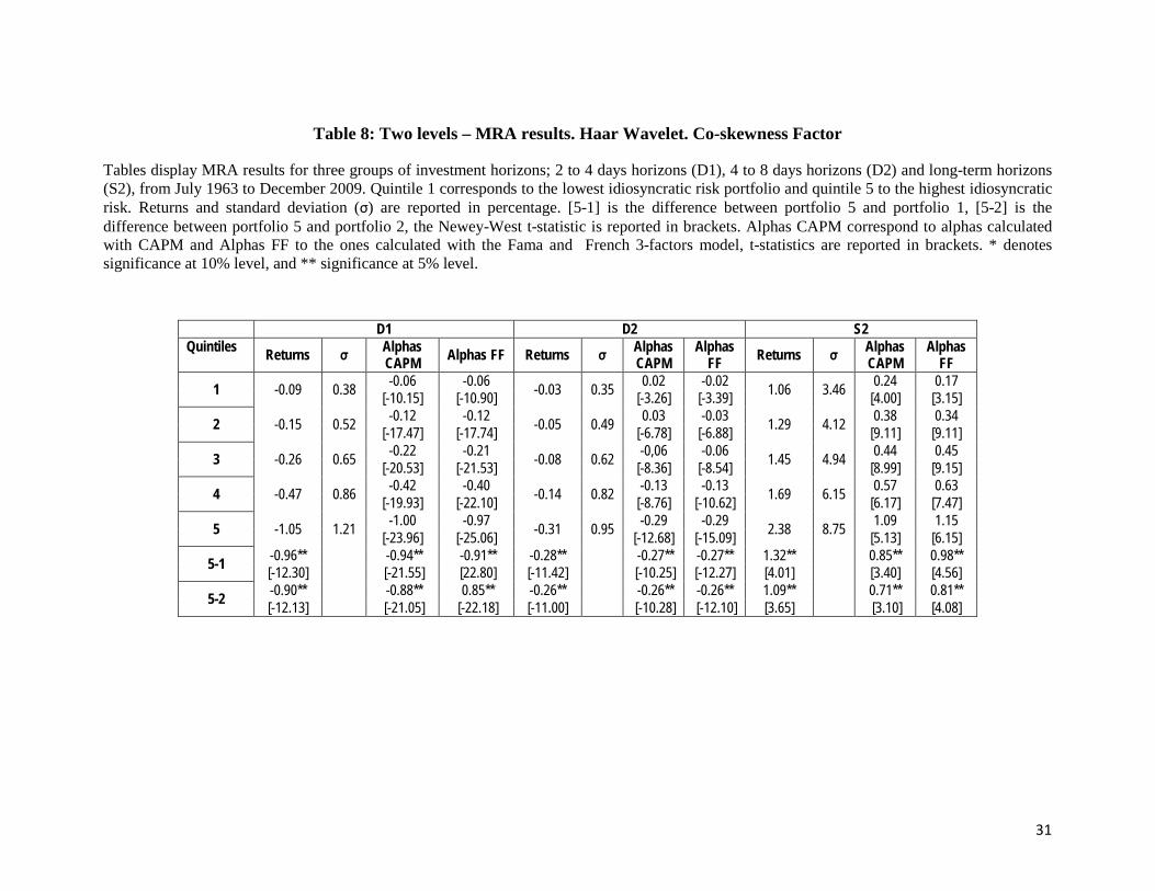
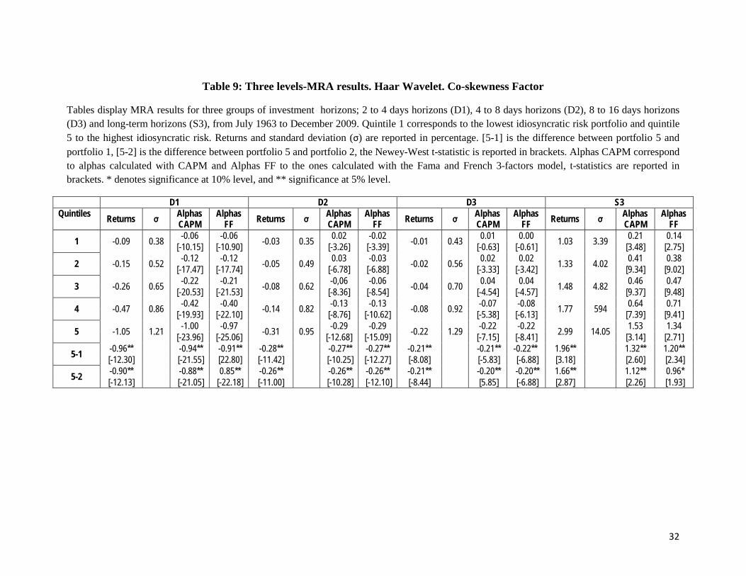
Despite the promising elements that lead us introducing the coskewness factor into

our analysis, Tables 7 to 9 provide evidence against its relevance in explaining the puzzle

existence for short-term investors. Introducing the factor virtually has not impact on D1’s

[5-1] returns, equal to -0.96% and significant both considering and dropping coskewness.

Differences decreases are meaningless also for D2 and D3; from a significant -0.30% to a

significant 0.28% in the case of D2 and from a significant 0.24% to a significant -0.21% for

D3. Also, controlling for risk CAPM or FF factors do not alter results and linearity in

returns decrease is again observed. Moreover, the drop in returns for the fifth portfolio 15 Results are available upon request.

18

remains unchanged so that coskewness can be ruled out as an explanation for that

phenomenon.

[Tables 7, 8 and 9]

In the same vein we introduce an illiquidity factor given that literature has constantly

signaled it as a possible cause for the puzzle to be observed. Ang et al., (2006) control both

for illiquidity and coskewness separately but their approach did not include controlling for

both at the same time. We use Amihud’s illiquidity measure defined in equation [8] to build

a factor for illiquidity.

𝐴𝑚𝑖ℎ𝑡𝑖 = �𝑟𝑒𝑡𝑡𝑖�𝑉𝑜𝑙𝑡𝑖� , [8]

For all stocks having more than 200 observations each year Amihud’s measure is

calculated. Stocks are then sorted according to annual Amihud mean measure and are

assigned one of three portfolios. Factor’s value weighted returns are calculated for the next

day as the difference between the return on the highest illiquidity portfolio and the lowest

illiquidity portfolio. Here the cuts were also introduced so that each of the portfolios

contains 30% of the stocks. The procedure is repeated by rolling the initial window by one

day.

As shown on Tables 10 to 12 the inclusion of both factors into the analysis does not

account for the puzzle. As in the previous case decreases in [5-1] returns are small and the

negative relationship is still significant for all short-term investors.

[Tables 10, 11 and 12]

6. Conclusions

For classical asset pricing theory, the negative link between idiosyncratic risk and

expected returns established by Ang et al., (2006, 2009) is challenging so that its own

nature derives on the necessity of a radically different approach. We propose a

19

heterogeneous market framework that provides a possible theoretical explanation for the

puzzle and seems to fit empirical data features better. Our main conclusion is that the

puzzle reported above disappears for long-term horizons while holds for the short-term

ones. Our findings points out the relevance of the puzzle only for investors with short run

horizons as compared to those with short time horizons. This result holds when controlling

for different wavelet families and different idiosyncratic risk estimators including illiquidity

and coskewness effects. Moreover, adding several definitions of short-term investors

provides corroborating evidence to our hypothesis that the puzzle is related to investors’

time horizon. This is because the link between idiosyncratic risk and returns becomes

weaker as we increase the number of short-term investors groups.

References

Ang, A., Hodrick, R., Xing, Y., and Zhang, X. (2009). High idiosyncratic volatility and low returns: International and further U.S. evidence. Journal of Financial Economics (91), 1-23.

Ang, A., Hodrick, R., Xing, Y., and Zhang, X. (2006). The Cross-Section of Volatility and Expected Returns. The Journal of Finance , LXI (1), 259-299.

Asquith, P., Pathak, P., and Ritter, J. (2005). Short interest, institutional ownership and stock returns. Journal of Financial Economics (78), 2, 243-276

Bali, T., and Cakici, N. (2008). Idiosyncratic Volatility and the Cross-Section of Expected Returns? Journal of Financial and Quantitative Analysis (43), 29-58.

Berrada, T., and Hugonnier, J. (2010). Incomplete information, idiosyncratic volatility and stock returns. Swiss Finance Institute Research Paper Series N°08 – 23.

Blackledge, J. (2010). Systemic Risk Assessment using a Non-stationary Fractional Dynamic Stochastic Model for the Analysis of Economic Signals. ISAST Transactions on Computers and Intelligent Systems, (2), 1, 76 – 94.

Boehme, R., Danielsen, B., and Sorescu, S. (2006). Short sale constraints, difference of opinions and overvaluation. Journal of Financial and Quantitative Analysis, 41, 455-487.

Boyer, B., Mitton, T., and Vorkink, K. (2010). Expected idiosyncratic skewness. The Review of Financial Studies (23), 1, 169-202.

Bowdena, R.J. and Zhub, J. (2010). Multi-scale variation, path risk and long-term portfolio management. Quantitative Finance, 10 (7), 783-796.

Brailsford, T., and Faff, R. (1997). Testing the Conditional CAPM and the effect of intervalling: A note. Pacific-Basin Finance Journal (5), 527-537.

Brailsford, T., and Josev, T. (1997). The impact of the return interval on the estimation of systematic risk. Pacific-Basin Finance Journal (5), 357-376.

Brandt, M., Brav, A., Graham, J. and Kumar, A. (2008). The Idiosyncratic Volatility Puzzle: Time Trend or Speculative Episodes? McCombs Research Paper Series No. FIN-02-09.

Cao, X. and Xu, Y. (2010). Long-run Idiosyncratic Volatilities and Cross-Sectional Stock Returns. Working Paper Series. University of Texas.

Douglas, George W., 1969, Risk in the Equity Markets: An Empirical Appraisal of Market Efficiency, Yale Economic Essays (9), 3–45.

Epps, T. (1979). Comovements in the stock price in the very short time. Journal of the American Statistical Association , 74, 291-298.

21

Falkenstein, E. (1996). Preferences for Stock Characteristics as Revealed by Mutual Fund Portfolio Holdings. The Journal of Finance, 51 (1), 111-135.

Fama, E. and Macbeth, J. (1973). Risk, Return and Equilibrium: Empirical Tests, Journal of Political Economy (81), 607–636.

Fernandez, V. (2005). The International CAPM and a wavelet-based decomposition of Value at Risk?, Studies of Nonlinear Dynamics and Econometrics 9(4).

Frankel, J and Froot, K. (1990). Chartists, Fundamentalists and Trading in the Foreign Exchange Market, The American Economic Review, 80 (2), 181-185

Fu, F. (2009). Idiosyncratic risk and the cross-section of expected stock returns. Journal of Financial Economics, XCI, 24-37.

Galagedera D.U. and Maharaja E. (2008) , Wavelet timescales and conditional relationship between higher-order systematic co-moments and portfolio returns, Quantitative Finance 8 (2) 201-215

Gençay, R., Selcuk, F., and Whicher, B. (2003). Systematic risk and time scales. Quantitative Finance, 3, 108-116.

Gençay, R., Selcuk, F., and Whicher, B. (2005). Multiscale systematic risk. Journal of International Money and Finance, 24, 55-70.

Gençay, R., Selcuk, F., and Whicher, B. (2010). Assymetry of information flow between volatilities across time scales. Quantitative Finance, X , 8, 895-915.

Gil-Bazo, J., Moreno, J. D. and Tapia, M. (2007). Price Dynamics, Informational Efficiency and Wealth Distribution in Continuous Double Auction Markets. Computational Intelligence, 23 (2), 176-196.

Han, B. and Kumar, A. (2009). Speculation. Realization Utility, and Asset Prices. Working Paper. McCombs School of Business, University of Texas.

Handa, P., Kothari, S. and Wasley, C. (1993). Sensitivity of multivariate tests of the capital asset-pricing model to the return measurement interval. Journal of Finance 48, 1543-1551.

Hawawini, G. (1983). Why beta shifts as the return interval changes. Financial Analysts Journal , 39, 73-77.

Huang, S. and Wu, T. (2008). Wavelet-Based Relevance Vector Machines for Stock Index Forecasting. Expert Systems

Huang, J., Sialm, and Zhang, H. (2011). Risk shifting and mutual fund performance. Review of

Financial Studies

22

In F., Kim S., Marisetty V. and Faff R., (2008). Analyzing the performance of managed funds using the wavelet multiscaling method, Review Quantitative Finance Accounting 31(1):55-70

Kim, S., and In, F. (2005). The relationship between stock returns and inflation: new evidence from wavelet analysis. Journal of Empirical Finance 12 (3), 435–444hhr001

Kim, S., and In, F. (2010). Portfolio allocation and the investment horizon: a multiscaling approach, Quantitative Finance 10(4) 443-453

LeBaron, B. (2000). Agent-based computational finance: Suggested readings and early research. Journal of Economics Dynamics and Control, 24, 679-702.

Lehmann, B. N. (1990). Residual Risk Revisited, Journal of Econometrics (45), 71–97.

Levhari, D. and Levy, H. (1977). The Capital Asset Pricing Model and the Investment Horizon. The Review of Economics and Statistics, (59), 1, 92 – 104.

Lévy, M., Lévy, H and Solomon, S. (2000). Microscopic Simulation of Financial Markets : From Investor Behavior to Market Phenomena. Academic Press.

Lintner, J. (1965). Security Prices and Risk: The Theory and Comparative Analysis of A.T.andT. and Leading Industrials, presented at the Conference on “The Economics of Regulated Public Utilities” at the University of Chicago Business School.

Los, C.,A. (2003). Financial Market Risk: Measurement and analysis. Routledge.

Malkiel, B. and Xu, Y. (2002). Idiosyncratic risk and security returns. AFA 2001 New Orleans Meetings.

Mallat, S. (1989). A Theory for Multiresolution Signal Decomposition: the Wavelet Representation. IEEE Transactions on Pattern Analysis and Machine Intelligence (11), 674-693.

Mandelbrot, Benoit B. (1972). Statistical Methodology for Nonperiodic Cycles: From the Covariance to the R/S Analysis. Annals of Economic and Social Measurement 1(3), 259-290.

Masdemont J. and Ortiz-Gracia L., (2009). Haar Wavelets-Based Approach for Quantifying Credit Portfolio Losses, Quantitative Finance.

Merton, R. (1987). Presidential address: a simple model of capital market equilibrium with incomplete information. Journal of Finance (42), 483-510.

Miller, M., and Myron Scholes. (1972). Rates and Return in Relationship to Risk: A Re-examination of Some Recent Findings, in Michael C. Jensen, ed.: Studies in the Theory of Capital Markets, 47–78

23

Müller, U., Dacorogna, M., Davé, R., Olsen, R., Pictet, O., and Weiszäcker, J. (1997). Volatilities of dfifferent time resolutions - Analyzing the dynamics of market components. Journal of Empirical Finance , 4, 213-239.

Müller, U., Dacorogna, M., Davé, R., Pictet, O., Olsen, R., and Ward, J. (October 14-15th, 1993). Fractals and Intrinsic Time - A challenge to econometricians. XXXIXth Int AEA Conference on Real Time Econometrics. Luxembourg

Rhaiem, N., S. Ben Ammou and A. Ben Mabrouk, (2007). Wavelet Estimation of Systematic Risk at Different Time Scales Application to French Stock Market. The International Journal of Applied Economics and Finance, 1: 113-119

O’Hara, M. (2003). Liquidity and Price Discovery. The Journal of Finance. 58, 1335-1354.

Rua, A. and Nunes, Luís C., (2009). International comovement of stock market returns: A wavelet analysis, Journal of Empirical Finance, 16(4), 632-639.

Yanqin, F. and Gençay, S. (2010). Unit root tests with wavelets. Econometric Theory, 26, 1305-1331.

24

Table 1: Returns of Portfolios sorted by Idiosyncratic Risk

This table reports the results we obtain by replicating Ang et al., (2006) using data from July 1963 to December 2009. Quintile 1 corresponds to the lowest idiosyncratic risk portfolio and quintile 5 to the highest idiosyncratic risk. Returns and standard deviation (Std Dev) are reported in monthly percentage. The row [5-1] is the difference between portfolio 5 and portfolio. The Newey-West t-statistic is reported in brackets. Alphas CAPM correspond to Jensen’s alphas calculated with respect to the CAPM and Alphas FF with respect to the Fama and French 3-factors model. The t-statistics are reported in brackets. * denotes significance at 10% level, and ** significance at 5% level.

Quintile Returns Std Dev Alphas CAPM Alphas FF

1 0.88 3.58 0.12 0.04 [1.77] [0.71]

2 1.01 4.55 0.13 0.09 [2.56] [1.93]

3 1.10 5.83 0.11 0.13 [1.46] [1.85]

4 0.88 7.56 -0.23 -0.22 [-1.69] [-2.08]

5 0.22 9.19 -0.96 -1.00 [-4.21] [-5.69]

[5-1] -0.66* -1.08** -1.04** [-1.82] [-3.93] [-4.97]

25

Table 2: Evidence of the puzzle using Carhart (1997)

Table reports the results using the Carhart (1997) model for data sample July 1963 to December 2000. Quintile 1 corresponds to the lowest idiosyncratic risk portfolio and quintile 5 to the highest idiosyncratic risk. Returns and standard deviation (Std Dev) are reported in percentage. [5-1] is the difference between portfolio 5 and portfolio 1, [5-2] is the difference between portfolio 5 and portfolio 2, the Newey-West t-statistic is reported in brackets. Alphas CAPM correspond to alphas calculated with CAPM and Alphas FF4 to the ones calculated with the Carhat (1997) model, t-statistics are reported in brackets. * denotes significance at 10% level, and ** significance at 5% level.

Quintile Returns Std Dev Alphas CAPM Alphas FF

1 0.88 3.58 0.11 0.05 [1.75] [0.82]

2 1.02 4.55 0.14 0.10 [2,72] [2.08]

3 1.11 5.82 0.11 0.12 [1.46] [1.80]

4 0.92 7.56 -0.20 -0.18 [-1.40] [-1.69]

5 0.27 9.28 -0.92 -0.98 [-3,97] [-5.46]

[5-1] -0.61* -1.03** -1.03** [-1.70] [-3.72] [-4.81]

[5-2] -0.75** -1.06** -1.08** [-2.47] [-4.18] [-5.58]

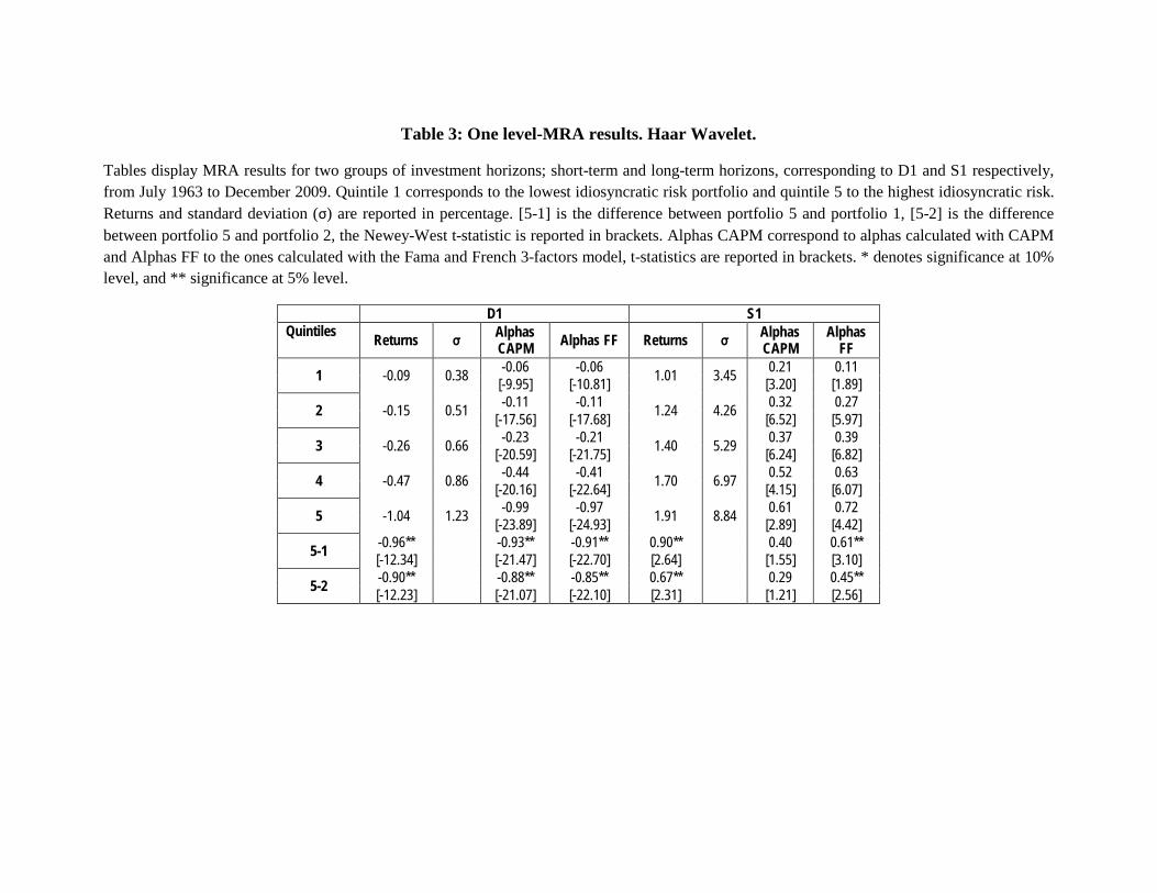
Table 3: One level-MRA results. Haar Wavelet.

Tables display MRA results for two groups of investment horizons; short-term and long-term horizons, corresponding to D1 and S1 respectively, from July 1963 to December 2009. Quintile 1 corresponds to the lowest idiosyncratic risk portfolio and quintile 5 to the highest idiosyncratic risk. Returns and standard deviation (σ) are reported in percentage. [5-1] is the difference between portfolio 5 and portfolio 1, [5-2] is the difference between portfolio 5 and portfolio 2, the Newey-West t-statistic is reported in brackets. Alphas CAPM correspond to alphas calculated with CAPM and Alphas FF to the ones calculated with the Fama and French 3-factors model, t-statistics are reported in brackets. * denotes significance at 10% level, and ** significance at 5% level.

D1 S1 Quintiles Returns σ Alphas

CAPM Alphas FF Returns σ Alphas CAPM

Alphas FF

1 -0.09 0.38 -0.06 -0.06 1.01 3.45 0.21 0.11 [-9.95] [-10.81] [3.20] [1.89]

2 -0.15 0.51 -0.11 -0.11 1.24 4.26 0.32 0.27 [-17.56] [-17.68] [6.52] [5.97]

3 -0.26 0.66 -0.23 -0.21 1.40 5.29 0.37 0.39 [-20.59] [-21.75] [6.24] [6.82]

4 -0.47 0.86 -0.44 -0.41 1.70 6.97 0.52 0.63 [-20.16] [-22.64] [4.15] [6.07]

5 -1.04 1.23 -0.99 -0.97 1.91 8.84 0.61 0.72 [-23.89] [-24.93] [2.89] [4.42]

5-1 -0.96** -0.93** -0.91** 0.90** 0.40 0.61** [-12.34] [-21.47] [-22.70] [2.64] [1.55] [3.10]

5-2 -0.90** -0.88** -0.85** 0.67** 0.29 0.45** [-12.23] [-21.07] [-22.10] [2.31] [1.21] [2.56]

27

Table 4: One level – MRA results. Daubechies 8 Wavelet.

Tables display MRA results for two groups of investment horizons; short-term and long-term horizons, corresponding to D1 and S1 respectively, from July 1963 to December 2009. Quintile 1 corresponds to the lowest idiosyncratic risk portfolio and quintile 5 to the highest idiosyncratic risk. Returns and standard deviation (σ) are reported in percentage. [5-1] is the difference between portfolio 5 and portfolio 1, [5-2] is the difference between portfolio 5 and portfolio 2, the Newey-West t-statistic is reported in brackets. Alphas CAPM correspond to alphas calculated with CAPM and Alphas FF to the ones calculated with the Fama and French 3-factors model, t-statistics are reported in brackets. * denotes significance at 10% level, and ** significance at 5% level.

D1 S1 Quintiles Returns σ Alphas

CAPM Alphas

FF Returns σ Alphas CAPM

Alphas FF

1 -0.11 0.38 -0.08 -0.08 1.00 3.46 0.20 0.10 [-11.54] [-12.40] [3,03] [1.70]

2 -0.17 0.53 -0.13 -0.13 1.25 4.27 0.34 0.28 [-18.60] [-18.70] [6.64] [6.10]

3 -0.29 0.66 -0.25 -0.24 1.32 5.22 0.30 0.34 [-21.93] [-22.66] [5.17] [5.86]

4 -0.54 0.92 -0.48 -0.46 1.63 6.98 0.46 0.56 [-20.51] [-22.22] [3.79] [5.54]

5 -1.18 1.13 -1.12 -1.09 1.75 8.96 0.45 0.57 [-24.26] [-24.97] [2.17] [3.53]

5-1 -1.07** -1.04** -1.01** 0.75** 0.25 0.47** [-12.12] [-21.83] [-22.70] [2.24] [1.01] [2.41]

5-2 -1.01** -0.98** -0.96** 0.50* 0.12 0.29* [-12.07] [-21.59] [-22.37] [1.74] [0.49] [1.66]

28

Table 5: Two levels – MRA results. Haar Wavelet.

Tables display MRA results for three groups of investment horizons; 2 to 4 days horizons (D1), 4 to 8 days horizons (D2) and long-term horizons (S2), from July 1963 to December 2009. Quintile 1 corresponds to the lowest idiosyncratic risk portfolio and quintile 5 to the highest idiosyncratic risk. Returns and standard deviation (σ) are reported in percentage. [5-1] is the difference between portfolio 5 and portfolio 1, [5-2] is the difference between portfolio 5 and portfolio 2, the Newey-West t-statistic is reported in brackets. Alphas CAPM correspond to alphas calculated with CAPM and Alphas FF to the ones calculated with the Fama and French 3-factors model, t-statistics are reported in brackets. * denotes significance at 10% level, and ** significance at 5% level.

D1 D2 S2 Quintiles Returns σ Alphas

CAPM Alphas FF Returns σ Alphas CAPM

Alphas FF Returns σ Alphas

CAPM Alphas

FF

1 -0.09 0.38 -0.06 -0.06 -0.03 0.34 0.02 0.02 1.04 3.46 0.20 0.12 [-9.90] [-10.78] [-3.17] [-3.30] [3.29] [2.15]

2 -0.15 0.51 -0.11 -0.11 -0.04 0.49 0.03 0.03 1.28 4.08 0.35 0.32 [-17.55] [-17.67] [-6.52] [-6.67] [8.01] [7.86]

3 -0.26 0.66 -0.22 -0.21 -0.07 0.62 -0.06 -0.06 1.44 4.83 0.42 0.43 [-20.54] [-21.72] [-8.62] [-8.89] [8.73] [8.92]

4 -0.47 0.86 -0.42 -0.41 -0.15 0.83 -0.13 -0.13 1.74 6.05 0.60 0.67 [-20.12] [-22.61] [-8.82] [-10.66] [6.45] [7.93]

5 -1.04 1.23 -0.99 -0.97 -0.32 0.97 -0.31 -0.30 2.34 8.68 1.00 1.07 [-23.84] [-24.88] [-12.83] [-15.42] [4.95] [6.04]

5-1 -0.96** -0.93** -0.91** -0.30** -0.29** -0.28** 1.30** 0.80** 0.95** [-12.34] [-21.42] [-22.66] [-12.20] [-10.39] [-12.46] [3.86] [3.32] [4.65]

5-2 -0.90** -0.88** -0.85** -0.28** 0.28** -0.27** 1.06** 0.65** 0.75** [-12.23] [-21.02] [-22.01] [-12.37] [-10.46] [-12.52] [3.54] [2.98] [4.03]

29

Table 6: Three levels-MRA results. Haar Wavelet.

Tables display MRA results for three groups of investment horizons; 2 to 4 days horizons (D1), 4 to 8 days horizons (D2), 8 to 16 days horizons (D3) and long-term horizons (S3), from July 1963 to December 2009. Quintile 1 corresponds to the lowest idiosyncratic risk portfolio and quintile 5 to the highest idiosyncratic risk. Returns and standard deviation (σ) are reported in percentage. [5-1] is the difference between portfolio 5 and portfolio 1, [5-2] is the difference between portfolio 5 and portfolio 2, the Newey-West t-statistic is reported in brackets. Alphas CAPM correspond to alphas calculated with CAPM and Alphas FF to the ones calculated with the Fama and French 3-factors model, t-statistics are reported in brackets. * denotes significance at 10% level, and ** significance at 5% level.

D1 D2 D3 S3 Quintiles Returns σ Alphas

CAPM Alphas

FF Returns σ Alphas CAPM

Alphas FF Returns σ Alphas

CAPM Alphas

FF Returns σ Alphas CAPM

Alphas FF

1 -0.09 0.38 -0.06 -0.06 -0.03 0.34 0.02 0.02 -0.01 0.42 0.00 0.00 1.00 3.29 0.17 0.10 [-9.90] [-10.78] [-3.17] [-3.30] [-0.48] [-0.45] [2.98] [1.87]

2 -0.15 0.51 -0.11 -0.11 -0.04 0.49 0.03 0.03 -0.03 0.55 0.02 0.02 1.32 4.00 0.39 0.34 [-17.55] [-17.67] [-6.52] [-6.67] [-3.55] [-3.77] [8.41] [8.03]

3 -0.26 0.66 -0.22 -0.21 -0.07 0.62 -0.06 -0.06 -0.04 0.71 0.03 0.03 1.54 4.88 0.50 0.50 [-20.54] [-21.72] [-8.62] [-8.89] [-4.28] [-4.31] [10.30] [10.20]

4 -0.47 0.86 -0.42 -0.41 -0.15 0.83 -0.13 -0.13 -0.08 0.94 -0.07 -0.07 1.91 6.30 0.72 0.81 [-20.12] [-22.61] [-8.82] [-10.66] [-5.06] [-5.88] [7.42] [9.39]

5 -1.04 1.23 -0.99 -0.97 -0.32 0.97 -0.31 -0.30 -0.25 1.30 -0.24 -0.24 4.05 26.45 2.29 1.74 [-23.84] [-24.88] [-12.83] [-15.42] [-7.91] [-9.15] [2.20] [1.64]

5-1 -0.96** -0.93** -0.91** -0.30** -0.29** -0.28** -0.24** -0.24** -0.24** 3.05** 2.12** 1.64 [-12.34] [-21.42] [-22.66] [-12.20] [-10.39] [-12.46] [-9.03] [-6.57] [-7.60] [2.59] [2.02] [1.54]

5-2 -0.90** -0.88** -0.85** -0.28** 0.28** -0.27** -0.22** -0.22** -0.22** 2.73** 1.90* 1.40 [-12.23] [-21.02] [-22.01] [-12.37] [-10.46] [-12.52] [-9.31] [-6.43] [-7.50] [2.38] [1.83] [1.33]

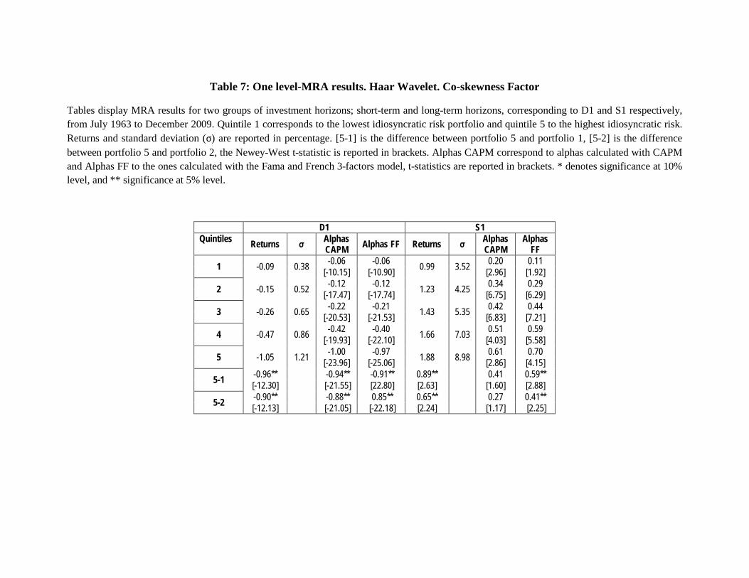
Table 7: One level-MRA results. Haar Wavelet. Co-skewness Factor

Tables display MRA results for two groups of investment horizons; short-term and long-term horizons, corresponding to D1 and S1 respectively, from July 1963 to December 2009. Quintile 1 corresponds to the lowest idiosyncratic risk portfolio and quintile 5 to the highest idiosyncratic risk. Returns and standard deviation (σ) are reported in percentage. [5-1] is the difference between portfolio 5 and portfolio 1, [5-2] is the difference between portfolio 5 and portfolio 2, the Newey-West t-statistic is reported in brackets. Alphas CAPM correspond to alphas calculated with CAPM and Alphas FF to the ones calculated with the Fama and French 3-factors model, t-statistics are reported in brackets. * denotes significance at 10% level, and ** significance at 5% level.

D1 S1 Quintiles Returns σ Alphas

CAPM Alphas FF Returns σ Alphas CAPM

Alphas FF

1 -0.09 0.38 -0.06 -0.06 0.99 3.52 0.20 0.11 [-10.15] [-10.90] [2.96] [1.92]

2 -0.15 0.52 -0.12 -0.12 1.23 4.25 0.34 0.29 [-17.47] [-17.74] [6.75] [6.29]

3 -0.26 0.65 -0.22 -0.21 1.43 5.35 0.42 0.44 [-20.53] [-21.53] [6.83] [7.21]

4 -0.47 0.86 -0.42 -0.40 1.66 7.03 0.51 0.59 [-19.93] [-22.10] [4.03] [5.58]

5 -1.05 1.21 -1.00 -0.97 1.88 8.98 0.61 0.70 [-23.96] [-25.06] [2.86] [4.15]

5-1 -0.96** -0.94** -0.91** 0.89** 0.41 0.59** [-12.30] [-21.55] [22.80] [2.63] [1.60] [2.88]

5-2 -0.90** -0.88** 0.85** 0.65** 0.27 0.41** [-12.13] [-21.05] [-22.18] [2.24] [1.17] [2.25]

31

Table 8: Two levels – MRA results. Haar Wavelet. Co-skewness Factor

Tables display MRA results for three groups of investment horizons; 2 to 4 days horizons (D1), 4 to 8 days horizons (D2) and long-term horizons (S2), from July 1963 to December 2009. Quintile 1 corresponds to the lowest idiosyncratic risk portfolio and quintile 5 to the highest idiosyncratic risk. Returns and standard deviation (σ) are reported in percentage. [5-1] is the difference between portfolio 5 and portfolio 1, [5-2] is the difference between portfolio 5 and portfolio 2, the Newey-West t-statistic is reported in brackets. Alphas CAPM correspond to alphas calculated with CAPM and Alphas FF to the ones calculated with the Fama and French 3-factors model, t-statistics are reported in brackets. * denotes significance at 10% level, and ** significance at 5% level.

D1 D2 S2 Quintiles Returns σ Alphas

CAPM Alphas FF Returns σ Alphas CAPM

Alphas FF Returns σ Alphas

CAPM Alphas

FF

1 -0.09 0.38 -0.06 -0.06 -0.03 0.35 0.02 -0.02 1.06 3.46 0.24 0.17 [-10.15] [-10.90] [-3.26] [-3.39] [4.00] [3.15]

2 -0.15 0.52 -0.12 -0.12 -0.05 0.49 0.03 -0.03 1.29 4.12 0.38 0.34 [-17.47] [-17.74] [-6.78] [-6.88] [9.11] [9.11]

3 -0.26 0.65 -0.22 -0.21 -0.08 0.62 -0,06 -0.06 1.45 4.94 0.44 0.45 [-20.53] [-21.53] [-8.36] [-8.54] [8.99] [9.15]

4 -0.47 0.86 -0.42 -0.40 -0.14 0.82 -0.13 -0.13 1.69 6.15 0.57 0.63 [-19.93] [-22.10] [-8.76] [-10.62] [6.17] [7.47]

5 -1.05 1.21 -1.00 -0.97 -0.31 0.95 -0.29 -0.29 2.38 8.75 1.09 1.15 [-23.96] [-25.06] [-12.68] [-15.09] [5.13] [6.15]

5-1 -0.96** -0.94** -0.91** -0.28** -0.27** -0.27** 1.32** 0.85** 0.98** [-12.30] [-21.55] [22.80] [-11.42] [-10.25] [-12.27] [4.01] [3.40] [4.56]

5-2 -0.90** -0.88** 0.85** -0.26** -0.26** -0.26** 1.09** 0.71** 0.81** [-12.13] [-21.05] [-22.18] [-11.00] [-10.28] [-12.10] [3.65] [3.10] [4.08]

32

Table 9: Three levels-MRA results. Haar Wavelet. Co-skewness Factor

Tables display MRA results for three groups of investment horizons; 2 to 4 days horizons (D1), 4 to 8 days horizons (D2), 8 to 16 days horizons (D3) and long-term horizons (S3), from July 1963 to December 2009. Quintile 1 corresponds to the lowest idiosyncratic risk portfolio and quintile 5 to the highest idiosyncratic risk. Returns and standard deviation (σ) are reported in percentage. [5-1] is the difference between portfolio 5 and portfolio 1, [5-2] is the difference between portfolio 5 and portfolio 2, the Newey-West t-statistic is reported in brackets. Alphas CAPM correspond to alphas calculated with CAPM and Alphas FF to the ones calculated with the Fama and French 3-factors model, t-statistics are reported in brackets. * denotes significance at 10% level, and ** significance at 5% level.

D1 D2 D3 S3 Quintiles Returns σ Alphas

CAPM Alphas

FF Returns σ Alphas CAPM

Alphas FF Returns σ Alphas

CAPM Alphas

FF Returns σ Alphas CAPM

Alphas FF

1 -0.09 0.38 -0.06 -0.06 -0.03 0.35 0.02 -0.02 -0.01 0.43 0.01 0.00 1.03 3.39 0.21 0.14 [-10.15] [-10.90] [-3.26] [-3.39] [-0.63] [-0.61] [3.48] [2.75]

2 -0.15 0.52 -0.12 -0.12 -0.05 0.49 0.03 -0.03 -0.02 0.56 0.02 0.02 1.33 4.02 0.41 0.38 [-17.47] [-17.74] [-6.78] [-6.88] [-3.33] [-3.42] [9.34] [9.02]

3 -0.26 0.65 -0.22 -0.21 -0.08 0.62 -0,06 -0.06 -0.04 0.70 0.04 0.04 1.48 4.82 0.46 0.47 [-20.53] [-21.53] [-8.36] [-8.54] [-4.54] [-4.57] [9.37] [9.48]

4 -0.47 0.86 -0.42 -0.40 -0.14 0.82 -0.13 -0.13 -0.08 0.92 -0.07 -0.08 1.77 594 0.64 0.71 [-19.93] [-22.10] [-8.76] [-10.62] [-5.38] [-6.13] [7.39] [9.41]

5 -1.05 1.21 -1.00 -0.97 -0.31 0.95 -0.29 -0.29 -0.22 1.29 -0.22 -0.22 2.99 14.05 1.53 1.34 [-23.96] [-25.06] [-12.68] [-15.09] [-7.15] [-8.41] [3.14] [2.71]

5-1 -0.96** -0.94** -0.91** -0.28** -0.27** -0.27** -0.21** -0.21** -0.22** 1.96** 1.32** 1.20** [-12.30] [-21.55] [22.80] [-11.42] [-10.25] [-12.27] [-8.08] [-5.83] [-6.88] [3.18] [2.60] [2.34]

5-2 -0.90** -0.88** 0.85** -0.26** -0.26** -0.26** -0.21** -0.20** -0.20** 1.66** 1.12** 0.96* [-12.13] [-21.05] [-22.18] [-11.00] [-10.28] [-12.10] [-8.44] [5.85] [-6.88] [2.87] [2.26] [1.93]

33

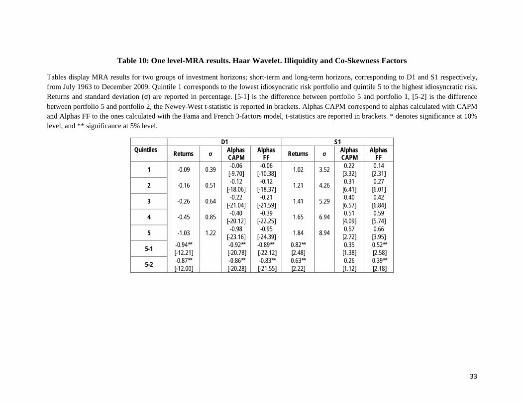
Table 10: One level-MRA results. Haar Wavelet. Illiquidity and Co-Skewness Factors

Tables display MRA results for two groups of investment horizons; short-term and long-term horizons, corresponding to D1 and S1 respectively, from July 1963 to December 2009. Quintile 1 corresponds to the lowest idiosyncratic risk portfolio and quintile 5 to the highest idiosyncratic risk. Returns and standard deviation (σ) are reported in percentage. [5-1] is the difference between portfolio 5 and portfolio 1, [5-2] is the difference between portfolio 5 and portfolio 2, the Newey-West t-statistic is reported in brackets. Alphas CAPM correspond to alphas calculated with CAPM and Alphas FF to the ones calculated with the Fama and French 3-factors model, t-statistics are reported in brackets. * denotes significance at 10% level, and ** significance at 5% level.

D1 S1 Quintiles Returns σ Alphas

CAPM Alphas

FF Returns σ Alphas CAPM

Alphas FF

1 -0.09 0.39 -0.06 -0.06 1.02 3.52 0.22 0.14 [-9.70] [-10.38] [3.32] [2.31]

2 -0.16 0.51 -0.12 -0.12 1.21 4.26 0.31 0.27 [-18.06] [-18.37] [6.41] [6.01]

3 -0.26 0.64 -0.22 -0.21 1.41 5.29 0.40 0.42 [-21.04] [-21.59] [6.57] [6.84]

4 -0.45 0.85 -0.40 -0.39 1.65 6.94 0.51 0.59 [-20.12] [-22.25] [4.09] [5.74]

5 -1.03 1.22 -0.98 -0.95 1.84 8.94 0.57 0.66 [-23.16] [-24.39] [2.72] [3.95]

5-1 -0.94** -0.92** -0.89** 0.82** 0.35 0.52** [-12.21] [-20.78] [-22.12] [2.48] [1.38] [2.58]

5-2 -0.87** -0.86** -0.83** 0.63** 0.26 0.39** [-12.00] [-20.28] [-21.55] [2.22] [1.12] [2.18]

34

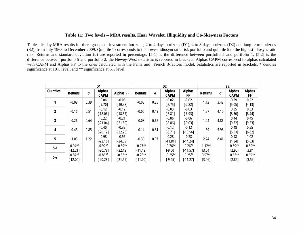
Table 11: Two levels – MRA results. Haar Wavelet. Illiquidity and Co-Skewness Factors

Tables display MRA results for three groups of investment horizons; 2 to 4 days horizons (D1), 4 to 8 days horizons (D2) and long-term horizons (S2), from July 1963 to December 2009. Quintile 1 corresponds to the lowest idiosyncratic risk portfolio and quintile 5 to the highest idiosyncratic risk. Returns and standard deviation (σ) are reported in percentage. [5-1] is the difference between portfolio 5 and portfolio 1, [5-2] is the difference between portfolio 5 and portfolio 2, the Newey-West t-statistic is reported in brackets. Alphas CAPM correspond to alphas calculated with CAPM and Alphas FF to the ones calculated with the Fama and French 3-factors model, t-statistics are reported in brackets. * denotes significance at 10% level, and ** significance at 5% level.

D1 D2 S2 Quintiles Returns σ Alphas

CAPM Alphas FF Returns σ Alphas CAPM

Alphas FF Returns σ Alphas

CAPM Alphas

FF

1 -0.09 0.39 -0.06 -0.06 -0.03 0.35 -0.02 -0.02 1.12 3.49 0.29 0.22 [-9.70] [-10.38] [-2.75] [-2.82] [5.05] [4.13]

2 -0.16 0.51 -0.12 -0.12 -0.05 0.49 -0.03 -0.03 1.27 4.10 0.35 0.33 [-18.06] [-18.37] [-6.81] [-6.93] [8.50] [8.44]

3 -0.26 0.64 -0.22 -0.21 -0.08 0.62 -0.06 -0.06 1.44 4.86 0.44 0.45 [-21.04] [-21.59] [-8.86] [-9.03] [9.32] [9.33]

4 -0.45 0.85 -0.40 -0.39 -0.14 0.81 -0.12 -0.12 1.59 5.98 0.48 0.55 [-20.12] [-22.25] [-8.71] [-10.56] [5.53] [6.82]

5 -1.03 1.22 -0.98 -0.95 -0.30 0.97 -0.28 -0.28 2.24 8.41 0.98 1.02 [-23.16] [-24.39] [-11.81] [-14.24] [4.84] [5.63]

5-1 -0.94** -0.92** -0.89** -0.27** -0.26** -0.26** 1.12** 0.69** 0.80** [-12.21] [-20.78] [-22.12] [-11.42] [-9.60] [-11.57] [3.64] [2.90] [3.84]

5-2 -0.87** -0.86** -0.83** -0.25** -0.25** -0.25** 0.97** 0.63** 0.69** [-12.00] [-20.28] [-21.55] [-11.00] [-9.45] [-11.27] [3.46] [2.85] [3.59]

35

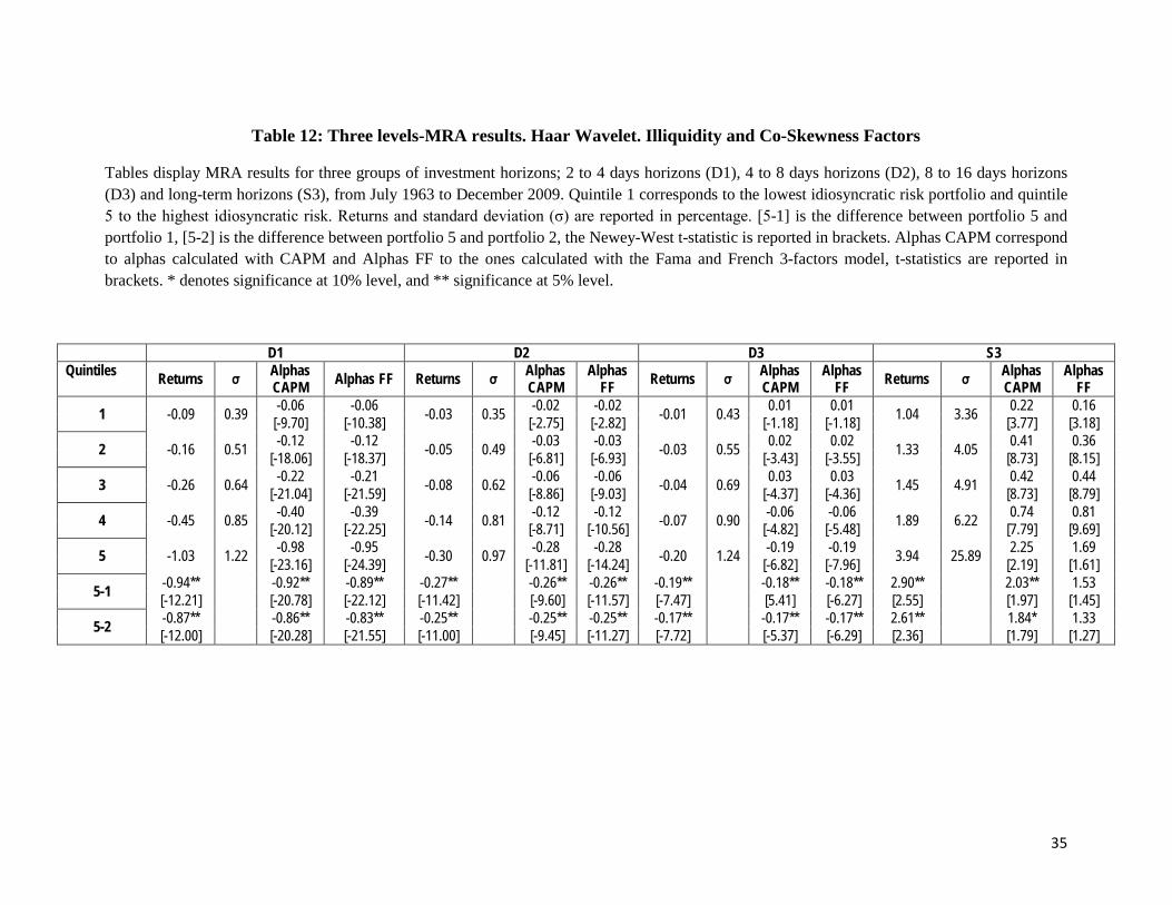
Table 12: Three levels-MRA results. Haar Wavelet. Illiquidity and Co-Skewness Factors

Tables display MRA results for three groups of investment horizons; 2 to 4 days horizons (D1), 4 to 8 days horizons (D2), 8 to 16 days horizons (D3) and long-term horizons (S3), from July 1963 to December 2009. Quintile 1 corresponds to the lowest idiosyncratic risk portfolio and quintile 5 to the highest idiosyncratic risk. Returns and standard deviation (σ) are reported in percentage. [5-1] is the difference between portfolio 5 and portfolio 1, [5-2] is the difference between portfolio 5 and portfolio 2, the Newey-West t-statistic is reported in brackets. Alphas CAPM correspond to alphas calculated with CAPM and Alphas FF to the ones calculated with the Fama and French 3-factors model, t-statistics are reported in brackets. * denotes significance at 10% level, and ** significance at 5% level.

D1 D2 D3 S3 Quintiles Returns σ Alphas

CAPM Alphas FF Returns σ Alphas CAPM

Alphas FF Returns σ Alphas

CAPM Alphas

FF Returns σ Alphas CAPM

Alphas FF

1 -0.09 0.39 -0.06 -0.06 -0.03 0.35 -0.02 -0.02 -0.01 0.43 0.01 0.01 1.04 3.36 0.22 0.16 [-9.70] [-10.38] [-2.75] [-2.82] [-1.18] [-1.18] [3.77] [3.18]

2 -0.16 0.51 -0.12 -0.12 -0.05 0.49 -0.03 -0.03 -0.03 0.55 0.02 0.02 1.33 4.05 0.41 0.36 [-18.06] [-18.37] [-6.81] [-6.93] [-3.43] [-3.55] [8.73] [8.15]

3 -0.26 0.64 -0.22 -0.21 -0.08 0.62 -0.06 -0.06 -0.04 0.69 0.03 0.03 1.45 4.91 0.42 0.44 [-21.04] [-21.59] [-8.86] [-9.03] [-4.37] [-4.36] [8.73] [8.79]

4 -0.45 0.85 -0.40 -0.39 -0.14 0.81 -0.12 -0.12 -0.07 0.90 -0.06 -0.06 1.89 6.22 0.74 0.81 [-20.12] [-22.25] [-8.71] [-10.56] [-4.82] [-5.48] [7.79] [9.69]

5 -1.03 1.22 -0.98 -0.95 -0.30 0.97 -0.28 -0.28 -0.20 1.24 -0.19 -0.19 3.94 25.89 2.25 1.69 [-23.16] [-24.39] [-11.81] [-14.24] [-6.82] [-7.96] [2.19] [1.61]

5-1 -0.94** -0.92** -0.89** -0.27** -0.26** -0.26** -0.19** -0.18** -0.18** 2.90** 2.03** 1.53 [-12.21] [-20.78] [-22.12] [-11.42] [-9.60] [-11.57] [-7.47] [5.41] [-6.27] [2.55] [1.97] [1.45]

5-2 -0.87** -0.86** -0.83** -0.25** -0.25** -0.25** -0.17** -0.17** -0.17** 2.61** 1.84* 1.33 [-12.00] [-20.28] [-21.55] [-11.00] [-9.45] [-11.27] [-7.72] [-5.37] [-6.29] [2.36] [1.79] [1.27]

36

Figure 1: Different partitions of the time – frequency plane according to the type of analysis

These plots dispolay division of the time-frequency plane for each type of time series analysis. Panel (a) shows the typical time series analysis in which the analysis focuses on the time appearance of phenomena. Panel (b) corresponds to Fourier Analysis. Here the relevant issue is which frequencies are present in the data and the time information is totally lost. Panel (c) shows the time-frequency division obtained by the Fourier Analysis and its dyadic scales; as seen in the figure, time support is divided by 2 each time scale is increased by 2j.

Signal y(t) constructed by three cosine functions with different frequencies: ω1=2/3, ω2=4 and ω3=2.

The three frequencies are quite well detected but the transform looses all information on the sequence of changes in frequency; time information is lost.

5 Level MRA. Original time series is the first. Scales are the following series. In each scale frequency components are identified for the time interval they appear on. Both frequency and time information are present

time

Freq

uenc

y

(a)

time

Freq

uenc

y

(b)

time

Freq

uenc

y

(c)