Time domain boundary element method for dynamic stress intensity factor computations

INTERNATIONAL JOURNAL FOR NUMERICAL METHODS IN ENGINEERING, VOL. 33,635-647 (1992)

TIME DOMAIN BOUNDARY ELEMENT METHOD FOR DYNAMIC STRESS INTENSITY FACTOR COMPUTATIONS

J. DOMINGUEZ AND R. GALLEGO.

Escuela Tkcnica Superior de lngenieros lndustriales, Universidad de Sevilla, Av. Reina Mercedes s/n, 41012-Sevilla, Spain

SUMMARY

This paper presents a procedure for transient dynamic stress intensity factor computations using traction singular quarter-point boundary elements in combination with the direct time domain formulation of the Boundary Element Method. The stress intensity factors are computed directly from the traction nodal values at the crack tip. Several examples of finite cracks in finite domains under mode4 and mixed mode dynamic loading conditions are presented. The computed stress intensity factors are represented versus time and compared with those obtained by other authors using different methods. The agreement is very good. The results are reliable and little mesh dependent. These facts allow for the analysis of dynamic crack problems with simple boundary discretizations. The versatile procedure presented can be easily applied to problems with complex geometry which include one or several cracks.

INTRODUCTION

The stress intensity factor (SIF) plays an important role in fracture studies and a lot of research effort has been put in developing methods for its computation. On the other hand, there is a considerable number of fracture mechanics problems for which the inertia effects are important and the need for dynamic analysis is obvious. Analytical solutions for dynamic fracture problems are limited to a small number of infinite domain problems. Numerical methods are the alternative for finite and irregular domains. Among the numerical methods used for dynamic SIF computations, the Finite Differences Method (FDM) and the Finite Element Method (FEM) have been well known for years. More recently the Boundary Element Method (BEM) has appeared as an efficient alternative for both static and for dynamic fracture mechanics. Interesting review papers of numerical solution techniques in dynamic fracture mechanics are those published by Kanninen' and more recently by Beskos.2

The direct formulation of the BEM was used in combination with singular quarter-point (SQP) elements to compute SIF of static linear elastic problems. Blandford et aL3 and Martinez and Dominguez4 showed that very accurate results are obtained with simple BE meshes. More recently Chirino and Dominguezs computed dynamic SIF in the frequency domain using the direct BEM formulation and SQP elements. They presented results for finite cracks in finite and infinite domains under harmonic load as well as under transient load obtained using the Fourier Transform. The possibilities and efficiency of the approach for static and frequency domain SIF computation were clearly established in those papers. Nevertheless, the area of dynamic fracture mechanics for which the BEM is more promising than the FDM and the FEM is crack

*Presently at Brown University

0029-598 1/92/030635-13$06.50 0 1992 by John Wiley & Sons, Ltd.

Received 12 October 1990 Revised 7 January 1991

636 J. DOMINGUEZ AND R. GALLEGO

propagation. For those problems, which require the analysis of a changing configuration, the process of mesh transformation should be much simpler in the BEM than in any domain technique. The reliable computation of dynamic SIF using a time domain step by step BEM is a necessary advance for the BE analysis of dynamic crack propagation problems.

The preliminary work of Nicholson and Mettu6S7 in this field should be mentioned. They presented two papers in which the time domain BEM is applied to compute mode4 dynamic SIF. They use two types of elements, one with constant interpolation functions in space and time and the other with interpolation functions quadratic in space and linear in time. For the first type of elements they obtained results that may be considered as good, taking into account the kind of elements used and the way the SIF is computed from the displacements given by the constant elements. Those authors do not recommend the use of their quadratic elements because they obtain poor results that show an anomalous oscillatory behaviour. A more precise and reliable approach than the use of constant elements to compute SIF is obviously needed.

In the present paper, the time domain formulation of the BEM is used to compute dynamic SIF under transient load. The elements are three-node quadratic in space combined with SQP elements for the crack tips. A time step by step approach is followed assuming piecewise constant and piecewise linear variation in time for tractions and displacements, respectively. Results for finite cracks in finite domains under mode-I and mixed mode dynamic loading conditions are computed. The stress intensity factors are obtained directly from the tip nodal values of the SQP elements. The SIF computed in this paper are compared with those obtained by other authors using different procedures. The computed results are very accurate, do not present oscillations and show very little dependency on the space and time discretization even in cases where FE results present oscillations.

The main differences between the present approach and that presented by Nicholson and M e t t ~ ~ , ~ are: first, a fully two-dimensional formulation with a two-dimensional fundamental solution is used in the present paper instead of considering the problems to be infinite length cylinders and using a three-dimensional fundamental solution as those authors do; second, SQP elements, which allow for the direct computation of the SIF from the tip nodal values, are used for the crack tips instead of using regular quarter-point elements and computing the SIF from the crack opening displacements; third, the singular kernels appearing when the source and receiver points lie in the same element are integrated analytically instead of using a 20-points Gauss scheme as Nicholson and Mettu do; and finally, piecewise constant and piecewise linear variation in time for tractions and displacements, respectively, are assumed in the present paper instead of using piecewise linear variation for both types of variables. This latter difference is possibly the main reason why the results presented in Reference 7 oscillate and those presented in this paper do not. The authors have found, in agreement with Cole et aL,* that when piecewise linear variation is used for both types of variables, the time stepping scheme is unstable. An explanation of this effect may be found in Reference 8.

Considerable work is also done these days with BE formulations for crack problems using integral equations with singularities stronger than those needed in the present work. Nishimura and Kobayashig and Krishnasamy et aE. * have presented hypersingular formulations for static and dynamic crack problems which do not require substructuring the body containing the crack. However, some kind of regularization of the strongly singular expressions is needed. This fact makes the methods based on those formulations more involved and only solutions to simple particular problems have been presented. The regular formulation, which yields accurate results for a variety of applications, is used in the present paper, because of its simplicity, reliability and easy numerical treatment.

DYNAMIC STRESS INTENSITY FACTORS 637

BASIC EQUATIONS

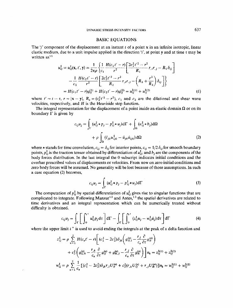
The ‘j’ component of the displacement at an instant t of a point x in an infinite isotropic, linear elastic medium, due to a unit impulse applied in the direction ‘i’, at point y and at time z may be written as”

1 u;j = .&(X, t’, y) = r , i r , j - R1dij

where t’ = t - 2, r = Ix - yI, R, = (c:tl2 - r2), c1 and c2 are the dilational and shear wave velocities, respectively, and ti is the Heaviside step function.

The integral representation for the displacement of a point inside an elastic domain R or on its boundary T is given by

P P

r + p (z7jou~jo - iijotiijo)dO

J R

where * stands for time convolution, cij = 6, for interior points, cij = 1/2 6, for smooth boundary points, p& is the traction tensor obtained by differentiation of u&; and b, are the components of the body forces distribution. In the last integral the 0 subscript indicates initial conditions and the overbar prescribed values of displacements or velocities. From now on zero initial conditions and zero body forces will be assumed. No generality will be lost because of those assumptions. In such a case equation (2) becomes,

c..u. = (uitj*pj - p!j*uj)dT (3) 1’ J j r

The computation of p b by spatial differentiation of u$ gives rise to singular functions that are complicated to integrate. Following Mansur’ and Antes,’ the spatial derivatives are related to time derivatives and an integral representation which can be numerically treated without difficulty is obtained.

cj juj = Ir [ I:+ u$pjdr] dT - Ir [ 1:’ (z&uj - wijtij)dz 1 dT (4)

where the upper limit t + is used to avoid ending the integrals at the peak of a delta function and

2 r


each one of the kernels z f j and wfj have been written as the sum of two terms corresponding to their two parts due to P- and S-waves, respectively (a = 1 and a = 2).

NUMERICAL FORMULATION

The numerical solution of equation (4) is done by discretization of the time into equal time steps At and of the boundary into boundary elements. Displacements and tractions are approximated using interpolation functions

where uyq and pyq stand for the jth displacement and traction, respectively, of the node q at the time t , = mAt. The functions @(r) and $¶(r) are space interpolation functions and p"(z) and q"(t) time interpolation functions.

The approximation for the velocities is taken consistently with that of the displacements:

In the present work the time interpolation functions pm(z) and qm(z) are assumed to be piecewise constant and piecewise linear, respectively. This choice has been proved to be very efficient as compared to other possibilities such as constant-constant or linear-1inear.l 2, l4

After the approximation, equation (4) for a boundary node p at the time step n takes the form

where Q is the total number of boundary nodes. The first time integral on the right-hand side of equation (7) can be written as

J r m - I

where U,!j"'(') and U,!jmm(2) are obtained by analytical integration of u& given by equation (1). The second time integral of equation (7) is written, following a similar notation, as

tt ( z&qm __ w&tj")dz = pc'"(1) + p t m ( 2 ) = p"P V (9) i.. 1

where P$"(l) and PGmC2) can be computed by analytical integration and algebraical condensation. The explicit expressions for UGmmfa) and PGmmfa) are as given by Antes.13 For the sake of brevity they are not reproduced here. Notice that the dependence of the above kernels on n and m is only on the difference n - m since uifj depends on the time difference t' = t - z.

The boundary element equation can now be written as n Q n Q

m = l q = l m = l q = l c5uj"P + C H,!jmPq~j"4 = 1 1 GtmPqpj"q (10)


where

GGmpq = Irq UGm(x, (n - m)At; xP)(pQ(r) dT

HGmpq = Jrq p f y ( x , (n - m)At; xp)$q(r) dT

The integrals along the boundary elements indicated in equation (1 1) are done by standard numerical integration except for the case when n = m and the collocation point p belongs to the integration element q. In such a case there are singularities in the kernels UGm and PGm for the instant t = t‘ = z = 0 and r = 0. Closed form expressions for those singular limits are given in Reference 15. The singularities in UGm and Pzm are the same as in elastostatics for r = 0, which are also the same that appear in frequency domain elastodynamics. In any other situation no singularities exist in the kernels UGm and PGm. It is worth noticing that if a piecewise constant time interpolation function had been assumed for the displacement, as other authors do,13 singularities of the type r- lI2 would have appeared at the front and the tail of each impulsive wave;16 i.e. for r = cat’ and r = ca(t’ - At). The numerical integration, in that case, requires more complicated approaches.

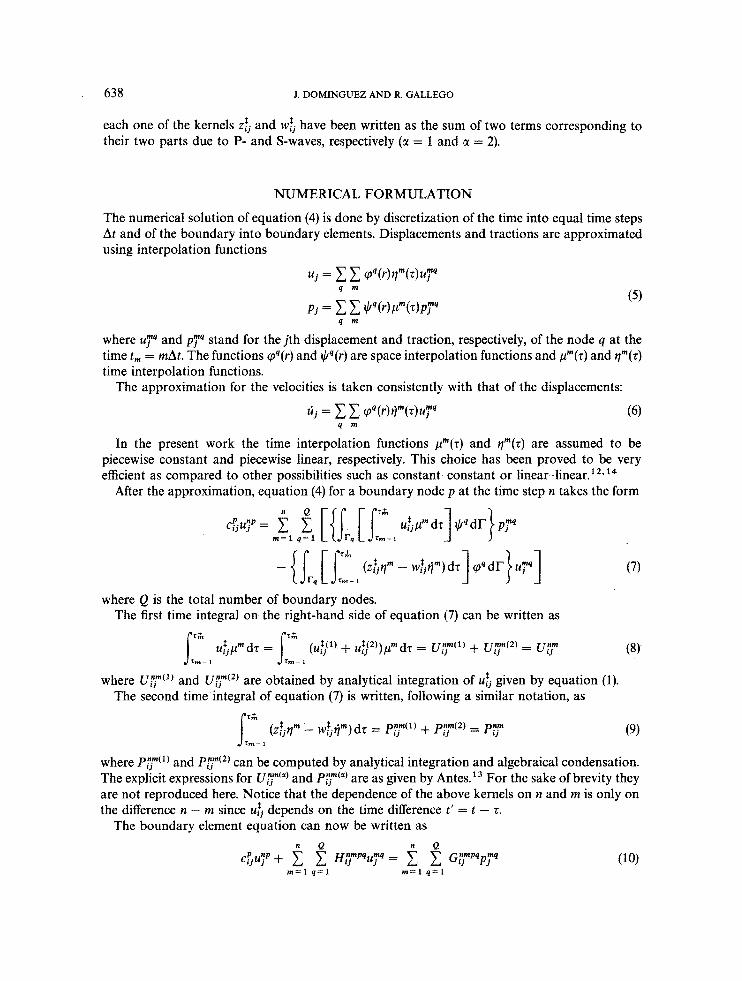
Two types of boundary elements are used in the present work. One is a standard three-node quadratic element, and the other is a singular quarter-point element which is described in more detail in the next section. The standard space quadratic element, its geometry, shape functions and other aspects of the formulation are the same as for elastostatics and may be found, for instance, in Reference 17. It will be mentioned here only that the numerical integration along the elements is done using a ten-points Gaussian quadrature except for the case when the wave front of the fundamental solution kernel is inside the integration element (Figure 1). In this case the integral extends only over that part of the element which has been reached by the wave and the number of Gauss points is increased up to sixteen because of the faster variation of the functions in this zone. When more than one wave front exists within the element (P- and S-waves), the location of both fronts is determined and the integration domain is divided into two parts, one reached only by the first wave and the other by both of them. Sixteen Gauss points are used for each part.

The space integration of the singular parts of the kernels along the element that contains the collocation point, during the first time step is done analytically using the same expressions of elastostatics.

Figure 1. Value of the Plz kernel along an element reached only by one wave


SINGULAR ELEMENT FOR SIF COMPUTATION

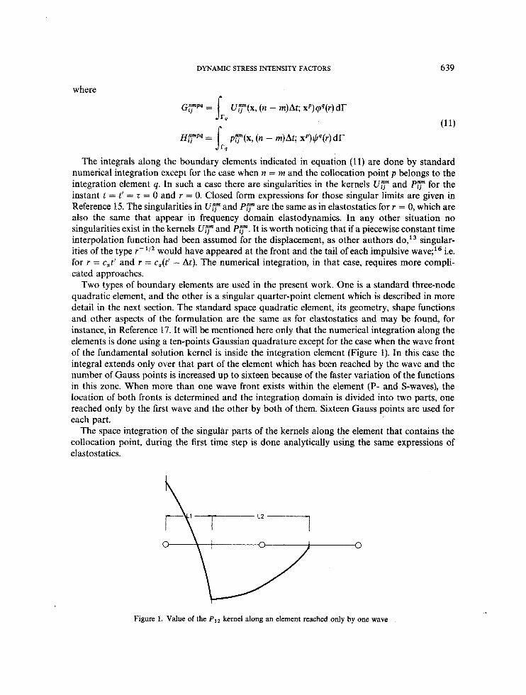
The SIF are computed using a singular quarter-point quadratic element in combination with subdivision of the domain into regions to avoid having the same equation for points on both sides of the crack. One singular quarter-point element is located at each side of the crack tips. The rest of the elements are standard quadratic elements. The present approach is based on the same ideas as the work previously presented in References 4 and 5 for elastostatics and frequency domain elastodynamics, respectively. The geometry, displacement and traction along a quadratic element may be represented as

where @, $ J ~ and (b3 are well known quadratic shape functions written in terms of the natural co-ordinate (Figure 2); f i represents a Cartesian component of the displacement, traction or geometry along the element, and fij is the value of that variable at node j .

When the quadratic element has a straight-line geometry and the mid-node is placed at a quarter of the length of the element, a simple relation between 5 and the variable r along the element (Figure 2) exists. Equation (12) may be written in terms of r as

fi = 4%' + @fi2 + 4 x 3 (12)

where

This kind of element is called a quarter-point element and is able to represent the ,/r behaviour of the displacement near the tip when one makes r coincide with r along one of the crack faces.

The singularity of the stress, and consequently of the traction, near the tip of the crack may be included in the representation of the traction by using modified quarter-point elements with singular shape functions:

ti = g4"+ i!#J2 $+ i ? 4 3 $ ti = i; $1 + f! $2 + f? $3 (15)

where tj are now the nodal values of ti divided by the nodal values of r@, i.e.

( a 1 (b)

Figure 2. Quadratic elements. Reproduced with permission from Int. j . numer. methods eng., 20, 1941-1950 (1984).

DYNAMIC STRESS INTENSITY FACTORS 64 1

and (1 5 ) written in terms of f is now c ,-.

where a,! = f!; 2: = -f? + 4ff - 3i! and a? = 2$ - 4tf + 2;;

The singular quarter-point boundary element includes a representation of the traction by means of (17) and a representation of the displacement by means of (13). Thus, both displacements and tractions may be represented, within the vicinity of the crack tip, by the first three terms of their series expansion.

The first and second mode stress intensity factors can be defined by the following limits:

K1 = lim (2nxl)112a22

KII = lim

x, -0

x i 4 0

If boundary discretization is carried out in such a way that the first element from the crack tip follows 9 = 0" and is a singular quarter-point boundary element, then, for this element, r = xl, t l = a12, t 2 = aZ2, and the nodal values for the tractions at the tip nilde k are

Thus, the stress intensity factors coincide with the traction nodal values except for a constant

and may be obtained directly from the computer code. Martinez and Dominguez4 showed for elastostatics how the use of the traction nodal values of the singular element at the crack tip is substantially less sensitive to the discretization than procedures that use a correlation formula of the crack opening displacement3 (COD).

CENTRE CRACKED PLATE UNDER MODE-I DYNAMIC LOAD

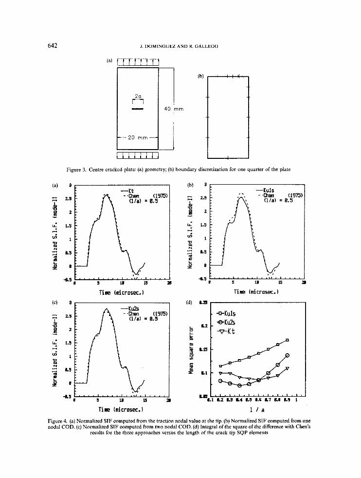
A rectangular plate with a central crack (see Figure 3(a)) is analysed. The plate is loaded dynamically along opposite boundaries at t = 0 by uniform tractions a with Heaviside-function time dependence. This problem was solved by Chen' using finite differences and has been frequently used as a reference to validate other methods. The material is linear elastic with properties as given by Chen: shear modulus p = 76 923 GPa, Poisson's ratio v = 0 3 and density p = 5000 kg/m3.

Because of the symmetry only one quarter of the plate is discretized, as shown in Figure 3(b). Two equal length elements are used to discretize one half of the crack (I/a = 0.5). The two elements that contain the tip are SQP. The time step At = 0.32 ps is such that P-waves travel 2.4 mm per time step. This corresponds approximately to twice the length of the smallest elements and one half of the largest. An analysis of the optimum time step and the effects of its changes may


Figure 3. Centre cracked plate: (a) geometry; (b) boundary discretization for one quarter of the plate

Tine hicrosec. 1 Time (microsec.)

(d) a=

*Kuls

0 L

~ ~ . ! * * . ~ ~ * ~ ~ * ~ ~ * . ~ ~ ~ . ~ ~ ~ ~ , ~ ~ ~ ~ . ~ ~ ~ ; ' Tine (microsec. 1 l i a

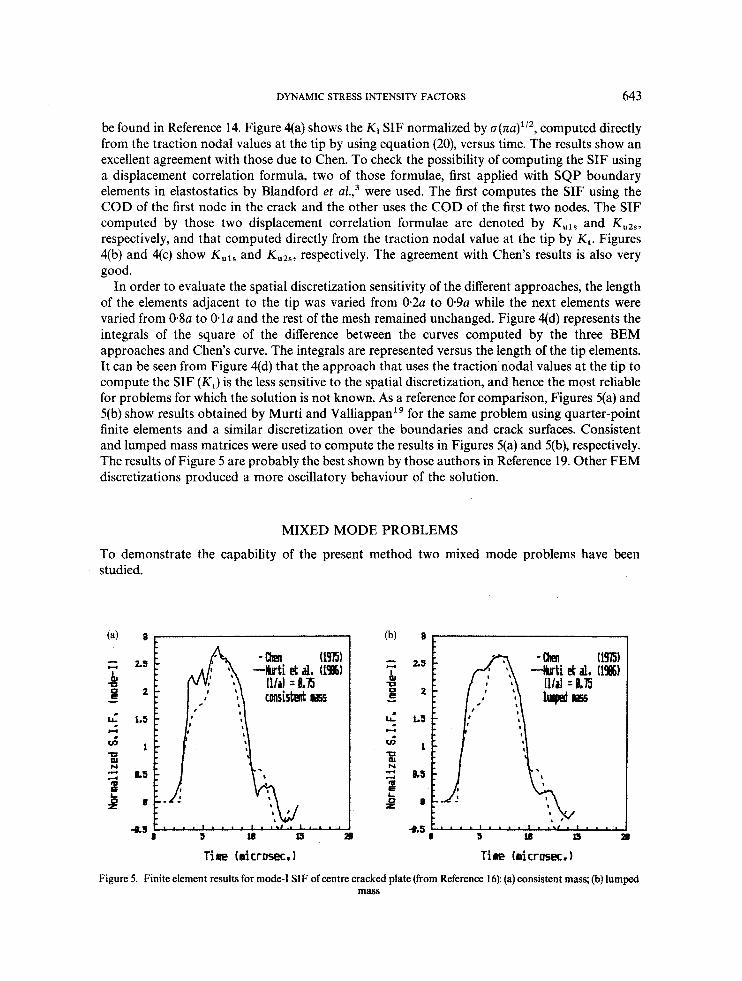
Figure 4. (a) Normalized SIF computed from the traction nodal value at the tip. (b) Normalized SIF computed from one nodal COD. (c) Normalized SIF computed from two nodal COD. (d) Integral of the square of the difference with Chen's

results for the three approaches versus the length of the crack tip SQP elements


be found in Reference 14. Figure 4(a) shows the K1 SIF normalized by ~(xu)'~', computed directly from the traction nodal values at the tip by using equation (20), versus time. The results show an excellent agreement with those due to Chen. To check the possibility of computing the SIF using a displacement correlation formula, two of those formulae, first applied with SQP boundary elements in elastostatics by Blandford et ~ l . , ~ were used. The first computes the SIF using the COD of the first node in the crack and the other uses the COD of the first two nodes. The SIF computed by those two displacement correlation formulae are denoted by Kuls and KU2%, respectively, and that computed directly from the traction nodal value at the tip by K , . Figures 4(b) and 4(c) show Kuls and KuZs, respectively. The agreement with Chen's results is also very good.

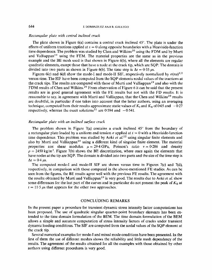
In order to evaluate the spatial discretization sensitivity of the different approaches, the length of the elements adjacent to the tip was varied from 0 . 2 ~ to 0 . 9 ~ while the next elements were varied from 0 . 8 ~ to Ola and the rest of the mesh remained unchanged. Figure 4(d) represents the integrals of the square of the difference between the curves computed by the three BEM approaches and Chen's curve. The integrals are represented versus the length of the tip elements. It can be seen from Figure 4(d) that the approach that uses the traction nodal values at the tip to compute the SIF ( K , ) is the less sensitive to the spatial discretization, and hence the most reliable for problems for which the solution is not known. As a reference for comparison, Figures 5(a) and 5(b) show results obtained by Murti and Vallia~pan'~ for the same problem using quarter-point finite elements and a similar discretization over the boundaries and crack surfaces. Consistent and lumped mass matrices were used to compute the results in Figures 5(a) and 5(b), respectively. The results of Figure 5 are probably the best shown by those authors in Reference 19. Other FEM discretizations produced a more oscillatory behaviour of the solution.

MIXED MODE PROBLEMS

To demonstrate the capability of the present method two mixed mode problems have been studied.

T i e (nicrosec. 1 Time (nicrosec. 1

Figure 5. Finite element results for mode-I SIF of centre cracked plate (from Reference 16): (a) consistent mass; (b) lumped mass


Rectangular plate with central inclined crack

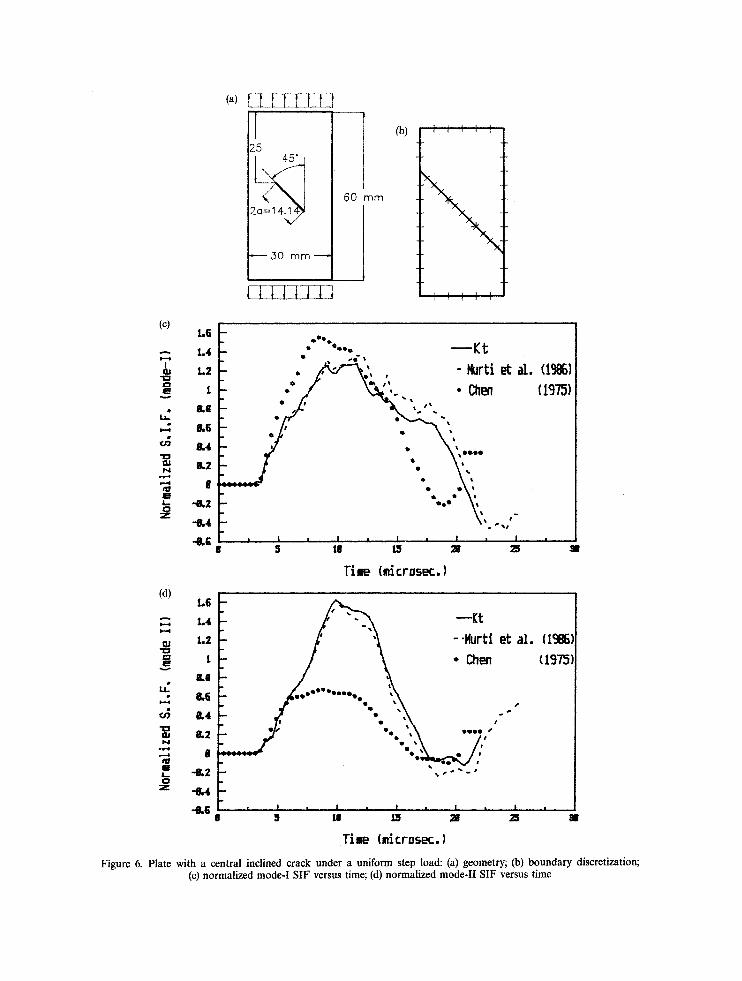
The plate shown in Figure 6(a) contains a central crack inclined 45”. The plate is under the effects of uniform tractions applied at t = 0 along opposite boundaries with a Heaviside-function time dependence. The problem was studied by Chen and Wilkins’’ using the FDM and by Murti and Valliappanig using the FEM. The material properties are the same as in the previous example and the BE mesh used is that shown in Figure 6(b), where all the elements are regular quadratic elements, except those that have a node at the crack tip, which are SQP. The domain is divided into two parts as shown in Figure 6(b). The time step is At = 0.35 ps.

Figures 6(c) and 6(d) show the mode-I and mode41 SIF, respectively normalized by C T ( E U ) ’ / ~

versus time. The SIF have been computed from the SQP elements nodal values of the tractions at the crack tips. The results are compared with those of Murti and Valliappan” and also with the FDM results of Chen and Wilkins.” From observation of Figure 6 it can be said that the present results are in good general agreement with the FE results but not with the FD results. It is reasonable to say, in agreement with Murti and Valliappan, that the Chen and Wilkins’O results are doubtful, in particular if one takes into account that the latter authors, using an averaging technique, computed from their results approximate static values of K , and KiI of 0.65 and -0-27 respectively, whereas the exact solutions2’ are 0594 and -0541.

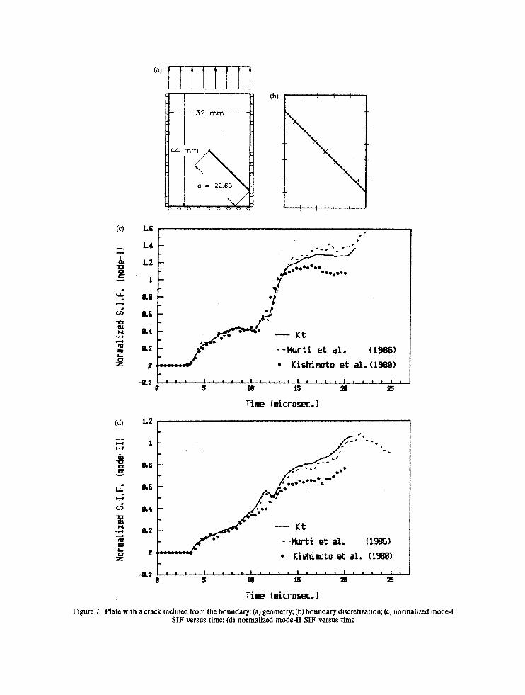
Rectangular plate with an inclined surface crack

The problem shown in Figure 7(a) contains a crack inclined 45” from the boundary of a rectangular plate loaded by a uniform end tension CT applied at t = 0 with a Heaviside-function time dependence. This problem was studied by Aoki et al.” using singular finite elements and also by Murti and Valliappan’9 using a different kind of singular finite element. The material properties are: shear modulus p = 29-4 GPa, Poisson’s ratio v = 0.286 and density p = 2450 kg/m3. Figure 7(b) shows the BE discretization, where once again the elements that have nodes at the tip are SQP. The domain is divided into two parts and the size of the time step is At = 0.4 ,US.

The computed mode-I and mode-I1 SIF are shown versus time in Figures 7(c) and 7(d), respectively, in comparison with those computed in the above-mentioned FE studies. As can be seen from the figures, the BE results agree well with the previous FE results. The agreement with the results obtained by Murti and Valliappan” is very good. The results due to Aoki et al. show some differences for the last part of the curves and in particular do not present the peak of KII at t = 11.5 p s that appears for the other two approaches.

CONCLUDING REMARKS

In the present paper a procedure for transient dynamic stress intensity factor computations has been proposed. The use of quadratic singular quarter-point boundary elements has been ex- tended to the time domain formulation of the BEM. The time domain formulation of the BEM allows a simple and accurate computation of stress intensity factors of cracks under transient dynamic loading conditions. The SIF are computed from the nodal values of the SQP element at the crack tip.

Several numerical examples for mode-I and mixed mode conditions have been presented. In the first of them the use of different meshes shows the reliability and little mesh dependency of the results. The agreement of the results obtained for all the examples with those obtained by other authors using different procedures is very good.

1.6

1.4

l.2

1

8.8

8 6

8.4

8.2

B &2

-084

4 6

1

25

2a=14.1 ~ 60 mrn

- 3 0 rnm-

1

et 111. t19e6l ( 19751

I I I I I I

8 9 18 19 as zi

Time (microsec. 1

Figure 6. Plate with a central inclined crack under a uniform step load (a) geometry; (b) boundary discretization; (c) normalized mode-I SIF versus time; (d) normalized mode-I1 SIF versus time

I

1.2 1 I- f .*--- -

K t - i u4

- - M u t i et al . (1986)

1.2

1

a a

0.6

a 4

0.2

8

-a2

Time (nicrosec.) Figure 7. Plate with a crack inclined from the boundary: (a) geometry; (b) boundary discretization; (c) normalized mode-I

SIF versus time; (d) normalized mode-I1 SIF versus time


In all cases the boundary discretization has been very simple as compared with the discretizations used for the FIE or FD studies. The method has been shown to be very versatile and can be used for more complicated geometries, including problems with several cracks.

ACKNOWLEDGEMENT

The authors would like to express their gratitude to the Spanish ‘Comision Interministerial de Ciencia y Tecnologia’ for supporting this work under a research grant.

REFERENCES

1. M. F. Kanninen, ‘A critical appraisal of solution techniques in dynamic fracture mechanics’, in A. R. Luxmore and D. R. J. Owen (eds.), Numerical Methods in Fracture Mechanics, Quadrant, Swansea, U.K., 1978, pp. 612434.

2. D. E. Beskos, ‘Numerical methods in dynamic fracture mechanics’, Research Report EUR 11300 EN, Ispra Establish- ment, European Joint Research Centre, 1987.

3. G. E. Blandford, A. R. Ingraffea and J. A. Liggett, ‘Two-dimensional stress intensity factor computations using the boundary element method’, Int. j . numer. methods eng., 17, 387-404 (1981).

4. J. Martinez and J. Dominguez, ‘On the use of quarter-point boundary elements for stress intensity factor computations’, Int. j . numer. methods eng., 20, 1941-1950 (1984).

5. F. Chirino and J. Dominguez, ‘Dynamic analysis of cracks using boundary element method‘, En@. Fract. Mech., 34,

6. J. W. Nicholson and S. R. Mettu, ‘Computation of dynamic stress intensity factors by the time domain integral

7. S. R. Mettu and J. W. Nicholson, ‘Computation of dynamic stress intensity factors by the time domain boundary

8. D. M. Cole, D. D. Kosloff and J. B. Minster, ‘A numerical boundary integral equation method for elastodynamics, 1’,

9. N. Nishimura and S. Kobayashi, ‘Regularised BIEs for miscellaneous elasticity problems’, in B. S. Annigeri and

10. G. Krishnasamy, L. W. Schmerr, T. J. Rudolphi and F. J. Rizzo, ‘Hypersingular boundary integral equations: some

1 1 . A. C. Eringen and E. S . Suhubi, Elastodynamics Vol. I I , Linear Theory, Academic Press, New York, 1975. 12. W. J. Mansur, ‘A time-stepping technique to solve wave propagation problems using the boundary element method’,

13. H. Antes, ‘A boundary element procedure for transient wave propagations in two-dimensional isotropic elastic

14. J. Dominguez and R. Callego, ‘On time domain boundary element method for elastodynamics’, Math. Comp.

15. R. Gallego, ‘Numerical studies of elastodynamic fracture mechanic problems’ (in Spanish). Ph.D. Thesis, Universidad

16. C. C Spyrakos and D. E. Beskos, ‘Dynamic response of rigid strip-foundations by a time-domain boundary element

17. C. A. Brebbia and J. Dominguez, Boundary Elements. An Introductory Course, Computational Mechanics Pub-

18. Y. M. Chen, ‘Numerical computation of dynamic stress intensity factor by Lagrangian finite-difference method’, Eng.

19. V. Murti and S. Valliappan, ‘The use of quarter point element in dynamic crack analysis’, Eng. Fract. Mech., 23,

20. Y. M. Chen and M. L. Wilkins, ‘Stress analysis of crack problems with a three dimensional time dependent computer program’, Int. J . Fract., 2, 607-617 (1976).

21. Y. Mukarami, ‘Analysis of mixed-mode stress intensity factors by body force method’, in D. R. J. Owen and A. R. Luxmore (eds.), Proc. 2nd Int. Con$ on Numerical Methods in Fracture Mechanics, Swansea, 1980, U.K., pp. 145-147.

22. S. Aoki, K. Kishimoto, Y. Izumihara and M. Sakata, ‘Dynamic analysis of cracked linear viscoelastic solids by finite element method using singular element’, Int. J . Fract., 16, 97-109 (1980).

105 1-1 061 (1 989).

equation method--1. Analysis’, Eng. Fract. Mech., 31, 759-767 (1988).

integral equation method-11. Examples’, Eng. Fract. Mech., 31, 769-782 (1988).

Bull. Seism. Soc. Am., 68, 1331-1357 (1978).

K. Tseng (eds.), Boundary Element Methods in Engineering, Springer-Verlag, Berlin, 1990.

applications in acoustic and elastic wave scattering’, 1. Appl. Mech. ASME, 57, 404-414 (1990).

Ph.D. Thesis, University of Southampton, U.K., 1983.

media’, Finite Elem. Anal. Des., I, 313-322 (1985).

Modelling, 15, 119-129 (1991).

de Sevilla, 1990.

method’, Int. j . numer. methods eng., 23, 1547-1565 (1986).

lications and McGraw-Hill, Southampton-New York, 1989.

Fract. Mech., 7, 653-660 (1975).

585-614 (1986).

Time domain boundary element method for dynamic stress intensity factor computations

Documents