Time-Dependent Resilience Assessment of Seismic Damage and ...

Time-Dependent Resilience Assessment ofSeismic Damage and Restoration ofInterdependent Lifeline Systems

Szu-Yun Lin, S.M.ASCE1; and Sherif El-Tawil, Ph.D., P.E., F.ASCE2

Abstract: A simulation of the resilience of lifeline systems in a test bed subjected to a series of seismic events is presented in this paper.The simulation framework is comprised of a group of independent simulators that interact through a publish–subscribe pattern for datamanagement. The framework addresses the spatial and time-dependent interactions that arise between lifeline systems as a hazard andsubsequent restoration processes unfold. The simulation results quantify how operability loss and recovery time may be underestimatedif the interdependencies between lifeline systems are not properly taken into account. The effect of insufficient resources on recovery wasinvestigated, and it was demonstrated that among the six resource allocation strategies studied, the time-varying strategies that are responsiveto actual conditions on the ground had a better effect on resilience. This paper demonstrates the power of connecting simulators usingthe publish–subscribe method in order to account for multiscale interdependency and time-dependent effects on community resilience.DOI: 10.1061/(ASCE)IS.1943-555X.0000522. © 2019 American Society of Civil Engineers.

Motivation and Objectives for the Study

Modeling a disaster and subsequent recovery efforts is complicatedby the differing time scales for the various phases of the process,that is, seconds or minutes as a hazard unfolds versus days ormonths as emergency efforts and recovery take place. As a result,studies that model the multiple phases of a disaster within oneoverarching simulation are rare due to the challenge of integratingdifferent simulation models with disparate temporal and spatialscales.

A common assumption in resilience studies is that a hazardoccurs during one analysis step, that is, virtually instantaneously.In reality, hazards unfold in a finite amount of time. Accounting forhow a hazard unfolds and affects infrastructure systems that interactwith one other can yield new insights into how interdependenciesaffect community resilience. This is especially important for sit-uations such as long-period disasters that overlap with short-termrecovery efforts [e.g., the emergency response to a hurricane(Schmeltz et al. 2013)], short-period disasters that interact withan ongoing recovery efforts (e.g., an aftershock affecting the re-covery effort associated with a main shock), or multiple disastersoccurring in a specific locale [e.g., an earthquake followed by atsunami (Moreno and Shaw 2019)].

Given the paucity of studies in this area, the objective of thisresearch was to conduct an analysis that explicitly addressed thespatial and temporal progression of earthquake-induced damageand the postdisaster restoration effort. After a review of the liter-ature, the methodology and framework are introduced and a case

study of three interdependent lifeline systems subjected to twosuccessive earthquakes is presented. Last, the applicability andlimitations of the framework are discussed.

Background

There is broad consensus that the interdependencies that exist be-tween the lifeline systems of a society can significantly impact theresilience of communities facing natural and man-made hazards(Cutter et al. 2003; NER 2011; Cimellaro et al. 2016).

Various methods for classifying interdependencies have beenproposed (Zimmerman 2001; Rinaldi et al. 2001; Dudenhoefferet al. 2006; Zhang and Peeta 2011), and different computationalmodeling approaches have been used to study the effects ofinterdependencies on community resilience. Eusgeld et al. (2008)and Ouyang (2014) categorized these approaches into severaltypes: empirical, agent-based, system dynamics, economic theory,network-based approaches, and other techniques. The two mostoften-used approaches for modeling community resilience areagent-based models and network-based methods. Agent-basedmodels are powerful because they can capture pertinent behaviorat the component level (Barton et al. 2000; Schoenwald et al. 2004;Reilly et al. 2017). Their versatility is, however, marred by theircomputational expense. Network-based approaches are computa-tionally expedient. They are widely used in lifeline system model-ing because these types of systems can typically be representedas a network graph with nodes and links (Hernandez-Fajardo andDuenas-Osorio 2013; Guidotti et al. 2016). A more detailed discus-sion of the various modeling techniques can be found in Eusgeldet al. (2008), Ouyang (2014), and Lin et al. (2019).

Numerous studies have been conducted to evaluate theresilience of communities subjected to hazards. The PEOPLESresilience framework (Renschler et al. 2010; Cimellaro et al. 2016)includes seven dimensions for assessing community resilience:population and demographics, environmental and ecosystem,organized governmental services, physical infrastructures, lifestyleand community competence, economic development, and social-cultural capital. Miles and Chang (2011) introduced a simulation

1Ph.D. Student, Dept. of Civil and Environmental Engineering, Univ. ofMichigan, Ann Arbor, MI 48109-2125 (corresponding author). ORCID:https://orcid.org/0000-0001-5369-2571. Email: [email protected]

2Professor, Dept. of Civil and Environmental Engineering, Univ. ofMichigan, Ann Arbor, MI 48109-2125. ORCID: https://orcid.org/0000-0001-6437-5176. Email: [email protected]

Note. This manuscript was submitted on January 21, 2019; approvedon July 15, 2019; published online on December 26, 2019. Discussionperiod open until May 26, 2020; separate discussions must be submittedfor individual papers. This paper is part of the Journal of InfrastructureSystems, © ASCE, ISSN 1076-0342.

© ASCE 04019040-1 J. Infrastruct. Syst.

J. Infrastruct. Syst., 2020, 26(1): 04019040

Dow

nloa

ded

from

asc

elib

rary

.org

by

Uni

vers

ity o

f Mic

higa

n on

07/

05/2

0. C

opyr

ight

ASC

E. F

or p

erso

nal u

se o

nly;

all

right

s res

erve

d.

model named ResilUS that was built on their previous efforts(Chang and Miles 2004; Miles and Chang 2007) and provided animplementation of the 1994 Northridge earthquake. The NIST-funded Center for Risk-Based Community Resilience Planninghas developed the Interdependent Networked Community Resil-ience Modeling Environment (IN-CORE), which some studieshave demonstrated on a virtual test bed community called Center-ville (Ellingwood et al. 2016; Guidotti et al. 2016; Lin and Wang2016; Cutler et al. 2016). The Civil Restoration with Interdepend-ent Social Infrastructure Systems (CRISIS) model (Loggins et al.2019) mapped services provided by civil infrastructure to theperformance of social infrastructure systems and aimed to find re-storation schemes that optimize the performance of social systems.As Koliou et al. (2018) concluded, there are only a handful offrameworks that can account for the multidisciplinary and multi-scale nature of community resilience in time-varying resilienceanalyses. The methodology employed in this research is gearedtoward addressing these gaps in the literature.

Computational Framework

Lin et al. (2019) provides a detailed description of the modelingenvironment and publish–subscribe data transmission pattern usedin this work. Fig. 1 shows how the various simulators employedherein interact together, and Fig. 2 illustrates the publish–subscriberelationship between the simulators. Each simulator publishes itsresults (in a “message”) to a corresponding “channel.” Other sim-ulators, which need the information, subscribe to the channelsand receive published messages from them. This method of datamanagement is used in computer science to compose complex sim-ulations from a set of individual, interacting simulators (Lin et al.2019). Modifiability and scalability are the key advantages of this

methodology. In particular, it allows simulators to be replacedbased on different theories or algorithms and permits new simula-tors to be added to existing simulation frameworks, allowing forincreasing levels of complexity.

The messages published during a disaster event are described inTable 1 and the corresponding publishers and subscribers are listedin Table 2. The run-time interface shown in Fig. 2 manages the flowof messages, permitting the analysis to proceed in a decentralizedand scalable manner. Although Figs. 1 and 2 show the frameworkfor the case study considered herein, which contains three inter-dependent systems, it can be extended in a straightforward mannerto handle other situations with more interacting systems andsimulators.

The scenario simulator in Fig. 1 describes the basic configura-tion information, specifically the location and characteristics of

Fig. 1. Simulation framework and message flow.

Fig. 2. Publish–subscribe concept for data exchange.

© ASCE 04019040-2 J. Infrastruct. Syst.

J. Infrastruct. Syst., 2020, 26(1): 04019040

Dow

nloa

ded

from

asc

elib

rary

.org

by

Uni

vers

ity o

f Mic

higa

n on

07/

05/2

0. C

opyr

ight

ASC

E. F

or p

erso

nal u

se o

nly;

all

right

s res

erve

d.

utility facilities and the connectivity between them. Such informa-tion is published at the beginning of simulations and assumed not tochange with time. Once a disaster occurs (in the disaster phase), thehazard intensity simulator provides information about the hazard,such as the magnitude and epicenter of an earthquake in a seismicdisaster. Although this paper only focuses on seismic events, thehazard intensity simulator could also provide information aboutstorm track and intensity if a hurricane hazard were of concern.The simulator provides specific hazard information at all locationsof interest to other simulators—for example, ground motions at agiven location.

The direct damage simulator calculates the physical damage ofcomponents directly induced by a hazard regardless of the influ-ence of other infrastructure systems. Damage can be evaluated us-ing empirical models, fragility curves, or detailed finite-elementmodels. The fact that the simulation framework does not care aboutthe specific method by which damage is assessed is a key strengthof the methodology. The interdependent damage simulator ad-dresses the effects of interdependencies on damage occurrence.Interdependencies come in many varieties. They can be functional,spatial, or both (Zimmerman 2001); cyber, geographic, and logical(Rinaldi et al. 2001); physical, geospatial, policy, and informational(Dudenhoeffer et al. 2006); functional, physical, budgetary, market,and economic (Zhang and Peeta 2011). The performance assess-ment simulator assesses system performance and is a key determi-nant for formulating a recovery strategy.

In the recovery phase, the recovery resource simulator estimatesthe amount of resources, such as labor, equipment, materials, and

budget, that can be used for lifeline restoration. The recovery strat-egy simulator allocates limited recovery resources to the systemsbased on a given recovery strategy, which may depend on the dam-age status and performance of the systems. The influencing factorsand strategy for the allocation of recovery resources may changeduring the recovery process. Such time-dependent effects are akey focus of this research; the study of such effects is enabledby the distributed simulation methodology adopted in this work.Once damage occurs, the physical recovery simulator determinesthe reconstruction priority of damaged components based on theirdamage situation and degree of importance in the system, and es-timates the required time for restoration. During every recoveryperiod, the simulator further distributes recovery resources allo-cated from the recovery strategy simulator to each damaged com-ponent in order of priority, that is, system level to component level.Then, within every recovery step, the physical recovery simulatordecides whether reconstruction progress advances forward orpauses according to whether a component has enough allocatedresources.

The interdependencies between the various systems must beconsidered not only as a hazard unfolds but also during the recov-ery process. For example, one component in a network system mayhave completely recovered from damage inflicted by a hazard butstill cannot function properly due to its dependency on anotherstill-damaged system. Therefore, like the interdependent damagesimulator, the interdependent recovery simulator considers inter-dependent behaviors across systems and updates the recoverystatus and functionality of components.

The simulators used in this work span different spatial scales:whole community, infrastructure system, and structural component.Community-level simulators affect large geographic areas (e.g., thescenario simulator and hazard intensity simulator) or represent de-cisions that address a large part of a community (e.g., the recoverystrategy simulator). System-level simulators address physical infra-structure systems such as lifeline networks. The lowest spatial levelpertains to components of the various infrastructure systems, suchas residential buildings or pumping stations. The times scalesconsidered herein also vary widely. As illustrated in Fig. 1, the timescale as the disaster phase unfolds Δthazard is several orders ofmagnitude smaller than the time step during the recovery phaseΔtrecovery. The framework employed in this work allows for thepossibility of subsequent hazards to occur—for example, an after-shock that occurs during an ongoing recovery progress.

Shifts between the disaster and recovery phases are controlledby the performance assessment simulator, which is involved in bothphases. This simulator judges the beginning and end of a disasterby interpreting the received damage messages and provides thelatest system performance to the recovery strategy simulator. Asshown in Fig. 1, in the disaster phase, the performance assessmentsimulator calculates system performance based on damage statusprovided by the interdependent damage simulator, and in the recov-ery phase, it continues to update system performance accordingto the recovery status from the interdependent recovery simulator.The direct damage simulator also subscribes to the recovery statusprovided by the interdependent recovery simulator, although it doesnot publish anything during the recovery phase. This is because itneeds to know the latest recovery status in order to assess the capac-ity reduction in components that are not yet fully repaired when thenext disaster occurs.

The computational framework handles several types of inter-dependencies. Most importantly, the interdependencies betweensystem performances and community-level recovery strategy areaccounted for in a dynamic sense. In other words, recovery strategycan evolve depending on system performance at a given time.

Table 1. Message types published during a disaster event

Code Message description

I Configuration of and information on test bed that does notchange with time

HðtÞ Hazard intensity measures at all locations of interest at time tDDi (t) Damage status of components directly induced by a hazard at

time tIDiðtÞ Damage status of components considering interdependency

effects at time tPi (t) System performance measures at time tRSðtÞ Total available recovery resources and constraints at time tSðtÞ Allocation strategy of recovery resources at time tRiðtÞ Physical recovery status of components at time tIRi (t) Recovery status of components considering interdependency

effects at time t

Note: Subscript i indicates messages produced by system i.

Table 2. Messages published or subscribed to by the simulators

SimulatorMessagepublished Messages subscribed to

Scenario simulator I —Hazard intensity simulator HðtÞ IDirect damage simulator i DDi (t) I, HðtÞ, IRj (t), j ¼ 1; 2; : : :Interdependent damagesimulator i

IDiðtÞ I, DDj (t), j ¼ 1; 2; : : :

Performance assessmentsimulator i

Pi (t) I, IDjðtÞ, IRj (t), j ¼ 1; 2; : : :

Recovery resource simulator RSðtÞ IRecovery strategy simulator SðtÞ I, Pj (t), j ¼ 1; 2; : : :Physical recovery simulator i RiðtÞ I, SðtÞInterdependent recoverysimulator i

IRi (t) I, RjðtÞ, j ¼ 1; 2; : : :

Note: Subscript i refers to system i.

© ASCE 04019040-3 J. Infrastruct. Syst.

J. Infrastruct. Syst., 2020, 26(1): 04019040

Dow

nloa

ded

from

asc

elib

rary

.org

by

Uni

vers

ity o

f Mic

higa

n on

07/

05/2

0. C

opyr

ight

ASC

E. F

or p

erso

nal u

se o

nly;

all

right

s res

erve

d.

Second, because additional disruptions can occur during an on-going recovery process, the ability of each component to resist newdemands caused by subsequent hazards may be affected by damagefrom a previous event and unfinished rehabilitation efforts. Last,interdependencies can occur between components of different life-line systems and must be accounted for. These interdependent re-lationships are shown in Fig. 1 by the interlaced lines joining thedirect damage simulator and the interdependent recovery simulatoror joining the physical recovery simulator and the interdependentrecovery simulator.

The extensibility and flexibility of the computational frameworkfor modeling various types of interdependencies between disparatesystems are the key strengths of the platform. For example, if newinteracting systems are added, the interdependent damage/recoverysimulators merely need to subscribe to the new direct damagesimulators or physical recovery simulators on which they depend.No changes need to be made to other simulators in the system. Thepublish–subscribe approach used in this work eliminates the needfor using interdependency matrices, which are commonly used tospecify the relationships between different pairs of networks. Thelimitations associated with using interdependency matrices arediscussed in Lin et al. (2019).

Case Study: Seismic Damage and Recovery ofLifeline Systems in Shelby County, Tennessee

Shelby County, Tennessee, which is close to the southwestend of the New Madrid seismic zone (NMSZ) has been used asa test bed in many studies. Duenas-Osorio et al. (2007), Adachi andEllingwood (2008), and Hernandez-Fajardo and Duenas-Osorio(2013) studied the interdependent response of water and powersystems in Shelby County under earthquake demands. Adachiand Ellingwood (2009) assessed the performance of its watersystem under spatially correlated seismic intensities. Song and Ok(2010) analyzed multiscale effects on system reliability of the gastransmission network in Shelby County. González et al. (2016)developed restoration strategies that took into account the interde-pendencies between the water, power, and gas network systems inShelby County.

In a departure from previous studies, the computational frame-work was applied to Shelby County, Tennessee in order to demon-strate how it can be used to investigate earthquake-induced damageand the subsequent recovery progress, which itself is interruptedby an aftershock (first shock—short term recovery effort—secondshock—long term recovery effort). The framework was appliedto three interdependent lifeline systems in order to demonstrateits scalability. Unlike the aforementioned studies, which merelyfocused on one of the phases in a hazard event, that is, the disasterprocess or the recovery period, this study presents an overallsimulation that addresses the disaster and postdisaster phases inan integrated manner. Another key advantage of the frameworkis that it naturally combines simulators that have disparate temporaland spatial scales.

To capture the uncertainty in the seismic damage and the resto-ration process, Monte Carlo simulations were performed, and themeans of the results are presented. Studies with 300, 500, and 1,000simulations were conducted to select a reasonable number of sim-ulations. The studies showed that the average relative differencesof the first to the last were 4.75% (300 runs versus 1,000 runs)and 0.21% (500 runs versus 1,000 runs). Therefore, the numberof Monte Carlo runs was set to 500.

The following section describes the details of the simulatorsshown in Fig. 1 and discussed previously.

Scenario Simulator

The scenario simulator provides configuration information aboutthe lifeline systems considered herein. The systems of interest in-clude the electric power system (EPS), water distribution system(WDS), and natural gas system (NGS), which are operated by theMemphis Light, Gas, and Water (MLGW) division. The topologi-cal configuration of the networks was adapted from Chang et al.(1996), Duenas-Osorio et al. (2007), and Song and Ok (2010).Fig. 3 shows the topologies and critical components of the power,water, and gas network systems in Shelby County. The gate stationsin EPS and NGS and the elevated tanks and pumping stations inWDS are supply nodes. The 23 kV/12 kV substations in EPS, theintersection nodes in WDS, and the regulator stations in NGS aredemand nodes. The intersection nodes in EPS and NGS and alldirected arcs represent the transmission components.

Hazard Intensity Simulator

The scenario earthquakes were assumed to have an epicenter at35°18’N and 90°18’W; the same assumption was made in Adachiand Ellingwood (2009). Ground motions designated RSN-5223(designated EQ1) and RSN-6536 (designated EQ2) from PEER(2018) were used in this study to represent feasible seismic activity.The ground motion records, which have a 0.01-s time interval, werescaled to peak ground acceleration (PGA) at the center of Memphis(35°08’N and 89°59’W; i.e., 33 km from the epicenter). The PGAvalues were 0.202 and 0.341 g for EQ1 and EQ2, respectively.These values were chosen based on USGS (2018) for earthquakeswith a 10% probability of exceedance in 50 years (10/50) and a 5%probability of exceedance in 50 years (5/50).

Ground motion attenuation was assumed to follow the modelproposed by Atkinson and Boore (1995). Although the attenuationrelationships were proposed only for the PGA, the model was as-sumed to be applicable to the entire acceleration record as plotted inFig. 4 and to depend only on the distance to the epicenter. Althoughthe assumptions related to the hazard were made for convenience,the hazard intensity simulator can be adjusted in the future oncemore data or new models become available.

Direct Damage Simulator

Direct damage occurs if the hazard intensity, as computed by thehazard intensity simulator, exceeds the capacity of a component.Four damage states are considered: minor, moderate, extensive,and complete. These states are irreversible and occur in sequentialorder. The capacity of each component is determined at the begin-ning of each realization in the Monte Carlo simulation. Lognormalfragility functions were used to estimate the capacities associatedwith different damage states for different types of utility facilities.The fragility functions were adopted from the Hazards US Multi-Hazard (HAZUS-MH) technical manual (FEMA 2003), and theirparameters are listed in Table 3. It was assumed that damage to EPScan be assessed from the gate stations and substations, which arethe most critical equipment for the functionality of a power system(Shinozuka et al. 2005). The intersection nodes in all networksadded for dividing the transmission lines and pipelines wereassumed to be not vulnerable to earthquakes (Fig. 3).

As discussed in FEMA (2003), the rate of occurrence of pipelinefailures per unit length is known as the repair rate and is computedvia Eq. (1), in which the unit for peak ground velocity (PGV) iscm=s. The probability that the number of pipe breaks NB equals bwithin a pipeline segment of length L can be expressed as shown inEq. (2), and the probability of pipeline breakage is shown in Eq. (3)

© ASCE 04019040-4 J. Infrastruct. Syst.

J. Infrastruct. Syst., 2020, 26(1): 04019040

Dow

nloa

ded

from

asc

elib

rary

.org

by

Uni

vers

ity o

f Mic

higa

n on

07/

05/2

0. C

opyr

ight

ASC

E. F

or p

erso

nal u

se o

nly;

all

right

s res

erve

d.

Rrate½repairs=km� ≅ 0.0001 × PGV2.25 ð1Þ

PðNB ¼ bÞ ¼ ðRrate × LÞbb!

e−Rrate×L ð2Þ

PðNB > 0Þ ¼ 1 − PðNB ¼ 0Þ ¼ 1 − e−Rrate×L ð3Þ

Each link in WDS and NGS is divided into several segments ofapproximately one km length in order to consider the scale effect(Song and Ok 2010). The PGV that corresponds with a 50%

Fig. 3. Topological configuration of the lifeline systems in Shelby County, Tennessee: (a) electric power; (b) water distribution; and (c) natural gassystem. [Adapted (a–c) from Chang et al. 1996; data for (a–b) from Duenas-Osorio et al. 2007; data for (c) from Song and Ok 2010.]

© ASCE 04019040-5 J. Infrastruct. Syst.

J. Infrastruct. Syst., 2020, 26(1): 04019040

Dow

nloa

ded

from

asc

elib

rary

.org

by

Uni

vers

ity o

f Mic

higa

n on

07/

05/2

0. C

opyr

ight

ASC

E. F

or p

erso

nal u

se o

nly;

all

right

s res

erve

d.

probability of pipeline breakage was used as the capacity of eachsegment. Buried pipelines may also be damaged by ground failure,for example, by liquefaction. Although such situations were notconsidered in this case study, they could be considered in the futureby adding other specialized simulators.

Component capacities are determined at the beginning of eachrealization based on the history of seismic activity. In the case of afirst seismic event, they are considered to be damage free. Whenaftershocks occur during the recovery process, the integrity of thesegments has already been compromised by the previous event, andcomponent capacities are assumed to be a function of the previousdamage state. In this case, the capacities of discrete componentswere assumed to be reduced by 40%, 20%, and 10% for extensive,moderate, and minor damage states, respectively, and the reductionratios for broken pipelines was set to 40%, that is, an extensivedamage state. These numbers can be refined in the future if the timebetween events is specified and the direct damage simulator andinterdependent recovery simulator are able to address sequentialdamage effects.

Interdependent Damage Simulator

Two types of interdependencies are considered at the component-level: functional interdependencies and spatial interdependencies.A functional interdependency indicates the dependence of one sys-tem (slave nodes) on the functionality or material flow of another(master nodes). For example, pumping stations in water and gassystems rely on electric power to operate pumping machines; elec-tric power plants rely on the water distribution system for coolingpurposes and for controlling emissions of coal-based power gener-ators. In this case study, part of the power grid depended on thenatural gas system to fuel generation units. Spatial interdependencyis a situation in which components from different infrastructuresystems are colocated within the same geographical environment,that is, the components have spatial overlap. There is generally

mutual reliance rather than master-slave relationship of functionalinterdependency; that is, the damage state of both nodes is the sameand is governed by the node that has more severe direct damage.

The conditional probability of a slave node being nonfunctionalgiven an inoperative master node can be seen as the degree of inter-dependency or the coupling strength between the two nodes.Herein, the conditional failure probability of any pair of slave andmaster nodes is set to one, but it can be adjusted for other situations.All these interdependent relationships and the nodes involved arelisted in Table 4. The interdependent damage simulator of eachsystem only needs to know which nodes are the master nodes ofits own components and subscribe to their damage conditions.

Performance Assessment Simulator

Ghosn et al. (2016) suggested that the performance measures ofa network system can be divided into two categories: flow-based

Table 3. Parameters of lognormal fragility functions for utility facilities

System Components Minor Moderate Extensive Complete

EPS Gate station 0.11 (0.50) 0.15 (0.45) 0.20 (0.35) 0.47 (0.40)12 kV/23 kV substation 0.15 (0.70) 0.29 (0.55) 0.45 (0.45) 0.90 (0.45)

WDS Elevated tanks 0.18 (0.50) 0.55 (0.50) 1.15 (0.60) 1.50 (0.60)Pumping station 0.15 (0.75) 0.36 (0.65) 0.77 (0.65) 1.50 (0.80)

NGS Gate station 0.15 (0.75) 0.34 (0.65) 0.77 (0.65) 1.50 (0.80)Regulator station 0.15 (0.75) 0.34 (0.65) 0.77 (0.65) 1.50 (0.80)

Note: All fragility functions for utility facilities are lognormal distributions with peak ground acceleration (PGA) as the engineering demand parameter. Thecorresponding median and lognormal standard deviation (β) are listed in the table, i.e., median (β); (unit: g).

Fig. 4. Assumed attenuation of ground acceleration (unit: g) for earthquake with (a) 5%; and (b) 10% probability of exceedance in 50 years.

Table 4. Interdependent relationships between EPS, WDS, and NGS

WDS*–EPS EPS*–WDS NGS*–EPS EPS*–NGSNGS–WDS(Mutual)

W2*–P28 P1*–W21 G6*–P18 P1*–G6 G3–W12W3*–P29 P2*–W25 G10*–P24 P5*–G11 G14–W41W4*–P14 P3*–W23 G12*–P44 P7*–G12 —W5*–P17 P4*–W29 G13*–P26 — —W6*–P33 P5*–W30 — — —W8*–P36 P6*–W35 — — —W9*–P38 P7*–W39 — — —W11*–P40 P8*–W42 — — —W12*–P26 P9*–W49 — — —

Note: The left four columns indicate functional interdependencies (slavenode*–master node), and the rightmost column indicates spatialinterdependencies.

© ASCE 04019040-6 J. Infrastruct. Syst.

J. Infrastruct. Syst., 2020, 26(1): 04019040

Dow

nloa

ded

from

asc

elib

rary

.org

by

Uni

vers

ity o

f Mic

higa

n on

07/

05/2

0. C

opyr

ight

ASC

E. F

or p

erso

nal u

se o

nly;

all

right

s res

erve

d.

and topology-based measures. Flow-based performance measuresare represented by the amount of supplied flow and the propor-tion of satisfied customer demand. Topology-based measures arecalculated based on graph theory. An abstract graph representinga lifeline network consists of supply nodes, demand nodes, and sev-eral directed links that indicate the connecting paths from supplynodes to demand nodes.

Due to a lack of information pertaining to flow capacity anddemand, a topology-based metric, termed connectivity loss (CL),was selected for performance assessment in this case study. CLmeasures the average change in the connectivity of demand nodesto supply nodes after perturbation and is often used to assess thecapability of a network system to withstand disruption (Albert et al.2004; Duenas-Osorio et al. 2007). At the beginning of a simulation,each lifeline system is represented as a graph with nodes and links,and the original connectivity is calculated. As the analysis pro-gresses, inoperative components are removed from the graph, thenadded back when they recover. CL of a network system withNdemand demand nodes can be computed by Eq. (4)

CL ¼ 1 − 1

Ndemand

XNdemand

i

�Pi

P0;i

�ð4Þ

where P0;i = original number of supply nodes that connect to the ithdemand node; and Pi = number of supply nodes connected to theith demand node after a perturbation. The remaining connectivity(C) of a network is: C ¼ 1 − CL.

Recovery Resource Simulator

Recovery resources are quantified as a number of resource units.A resource unit is defined as the amount of resources and budgetrequired for an 8-person crew with accompanying repair equipmentto work 12 hours (working time per day). In all of the case studiesdiscussed subsequently, the available number of resource unitsRtotal for the entire county was assumed to be a fixed value duringthe recovery process. In general, it is assumed that all crews haveunlimited expertise, that is, they can work on all lifeline systems.However, in last case study, the crews were assumed to have differ-ent skills, and the maximum number of available crews specializingin the ith lifeline system was denoted as Rmax;i. Clearly, the func-tionality of the social infrastructure—for example, the availabilityof able-bodied workers who were not injured or killed in theevent—affects Rmax;i. Although not accounted for here due to spaceand scope limitations, in the future, such a limitation can be ac-counted for through the addition of a social infrastructure simulatorthat, for example, accounts for worker injuries and deaths and foravailable funding needed to pay for repair crews.

Recovery Strategy Simulator

The recovery strategy simulator interprets the allocation strategyfor recovery resources. A feasible recovery strategy is to allocate

recovery resources to each system evenly regardless of their dam-age conditions, as stated in Eq. (5), where Ns is the number ofsystems and Rk is the amount of recovery resources allocated tothe kth system. This strategy (the EA strategy) could represent asituation in which information about the extent of a disaster isnot known. In cases in which Rtotal and Ns are fixed values duringthe recovery process, the EA strategy is time-independent

RkðtÞ ¼RtotalðtÞNs

ð5Þ

Another strategy (the LA strategy) is to assign resources de-pending on the performance of the systems in terms of connectivityloss. In this case, Rk is computed as

RkðtÞ ¼CLkðtÞPNsi CLiðtÞ

× RtotalðtÞ ð6Þ

where CLi = connectivity loss of the ith system. Alternatively, ifthe number of damaged components in each system NDi is of con-cern, then a feasible strategy (the DA strategy) could be as follows:

RkðtÞ ¼NDkðtÞPNsi NDiðtÞ

× RtotalðtÞ ð7Þ

The LA and DA strategies imply that the amount of recoveryresources allocated to each system is not constant and changes overtime t during the progress of recovery, reflecting the time-varyingcharacteristic of the recovery process.

The recovery strategies applied in the example assume thatsystems that are more severely damaged and have worse systemperformance will receive more recovery resources. However, deci-sion making during an actual disaster may be much more involvedand may need to account for other factors, such as economics,politics, and societal values. In such cases, users could refine thealgorithm in the recovery strategy simulator without influencingother simulators.

Physical Recovery Simulator

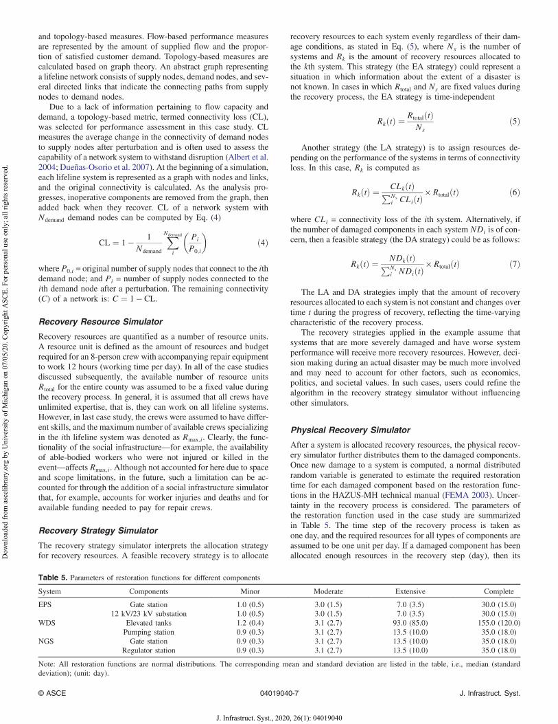
After a system is allocated recovery resources, the physical recov-ery simulator further distributes them to the damaged components.Once new damage to a system is computed, a normal distributedrandom variable is generated to estimate the required restorationtime for each damaged component based on the restoration func-tions in the HAZUS-MH technical manual (FEMA 2003). Uncer-tainty in the recovery process is considered. The parameters ofthe restoration function used in the case study are summarizedin Table 5. The time step of the recovery process is taken asone day, and the required resources for all types of components areassumed to be one unit per day. If a damaged component has beenallocated enough resources in the recovery step (day), then its

Table 5. Parameters of restoration functions for different components

System Components Minor Moderate Extensive Complete

EPS Gate station 1.0 (0.5) 3.0 (1.5) 7.0 (3.5) 30.0 (15.0)12 kV/23 kV substation 1.0 (0.5) 3.0 (1.5) 7.0 (3.5) 30.0 (15.0)

WDS Elevated tanks 1.2 (0.4) 3.1 (2.7) 93.0 (85.0) 155.0 (120.0)Pumping station 0.9 (0.3) 3.1 (2.7) 13.5 (10.0) 35.0 (18.0)

NGS Gate station 0.9 (0.3) 3.1 (2.7) 13.5 (10.0) 35.0 (18.0)Regulator station 0.9 (0.3) 3.1 (2.7) 13.5 (10.0) 35.0 (18.0)

Note: All restoration functions are normal distributions. The corresponding mean and standard deviation are listed in the table, i.e., median (standarddeviation); (unit: day).

© ASCE 04019040-7 J. Infrastruct. Syst.

J. Infrastruct. Syst., 2020, 26(1): 04019040

Dow

nloa

ded

from

asc

elib

rary

.org

by

Uni

vers

ity o

f Mic

higa

n on

07/

05/2

0. C

opyr

ight

ASC

E. F

or p

erso

nal u

se o

nly;

all

right

s res

erve

d.

repair progress will advance forward one day. Otherwise, it remainsunrepaired.

The physical recovery simulator distributes allocated recoveryresources to damaged components using two different strategies:randomly (the R strategy) or in order of their priority (the P strat-egy). In the latter case, the recovery priority of the components ineach network is as follows: supply nodes, demand nodes, and links/pipelines. To simplify the simulation, resources and work crew areassumed available as soon as they are allocated, that is, the effect oftransportation on work crew routing (Morshedlou et al. 2018) is notconsidered in this study, although it could be incorporated throughthe addition of other simulators.

Interdependent Recovery Simulator

The same types of interdependencies, that is, functional interdepen-dencies and spatial interdependencies, are considered during therecovery process by the interdependent recovery simulator. Theinterdependent relationships (master/slave) and involved nodes are

listed in Table 4. Although slave components may have completelyrecovered from damage inflicted by a hazard, they may not functionuntil the master components they depend on have fully recovered.For example, the functionality of pumping stations in the waterand gas systems depends both on their own repairs and on the avail-ability of electric power. After simulation of the physical recovery,the recovery status and functionality of components is updateddepending on the different interdependent behaviors across thesystems.

Results and Discussion

The simulators described in the previous section were connectedtogether using the computational framework described previously.The computational platform was then used to investigate the effectsof system interdependencies, multiple shocks, recovery strategies,and allocated recovery resources on the propagation of damageduring seismic events and short- and long-term recovery processes.

Fig. 5.Comparison of system performancewith and without considering interdependencies during the earthquake and recovery processes: (a) damagecurves of EPS; (b) recovery curves of EPS; (c) damage curves of WDS; (d) recovery curves of WDS; (e) damage curves of NGS; and (f) recoverycurves of NGS.

© ASCE 04019040-8 J. Infrastruct. Syst.

J. Infrastruct. Syst., 2020, 26(1): 04019040

Dow

nloa

ded

from

asc

elib

rary

.org

by

Uni

vers

ity o

f Mic

higa

n on

07/

05/2

0. C

opyr

ight

ASC

E. F

or p

erso

nal u

se o

nly;

all

right

s res

erve

d.

Interdependencies between Lifeline Systems

First, a comparison of the performance of the three lifeline systemswith and without considering the interdependencies between thesystems is presented. Consider a seismic event with EQ2, Rtotal ¼45 units=day, and crews with no limitation on their expertise. Theallocation of recovery resources is based on the LA and P strategies.Fig. 5 shows the damage and recovery curves of the three lifelinesystems in terms of the average system connectivity performance.The dotted lines in Fig. 5 reflect analyses that account for interde-pendencies, while the solid lines reflect simulations that do notaccount for interdependencies.

Figs. 5(a, c, and e) indicate that EPS is the system most signifi-cantly affected by the earthquake out of the three lifeline systemswhen interdependencies are not considered. Figs. 5(a and b) indi-cate that the performance of EPS is not significantly affected byinterdependencies. Interdependencies are much more influentialfor WDS and NGS, as shown in Figs. 5(c–e). The computationalresults show that WDS and NGS are more dependent on EPS,and the overall recovery time, in this case, is controlled by the re-storation of EPS. It is clear that the operability loss and recoverytimes may be significantly underestimated if the interdependenciesbetween lifeline systems are not adequately accounted for.

Fig. 6. Influence of foreshock on the lifeline system performance during (a) main shock without foreshock; (b) overall event without foreshock;(c) main shock affected by foreshock; and (d) overall event with foreshock.

Fig. 7. Influence of foreshock on recovery after main shock: (a) EPS; (b) WDS; and (c) NGS.

© ASCE 04019040-9 J. Infrastruct. Syst.

J. Infrastruct. Syst., 2020, 26(1): 04019040

Dow

nloa

ded

from

asc

elib

rary

.org

by

Uni

vers

ity o

f Mic

higa

n on

07/

05/2

0. C

opyr

ight

ASC

E. F

or p

erso

nal u

se o

nly;

all

right

s res

erve

d.

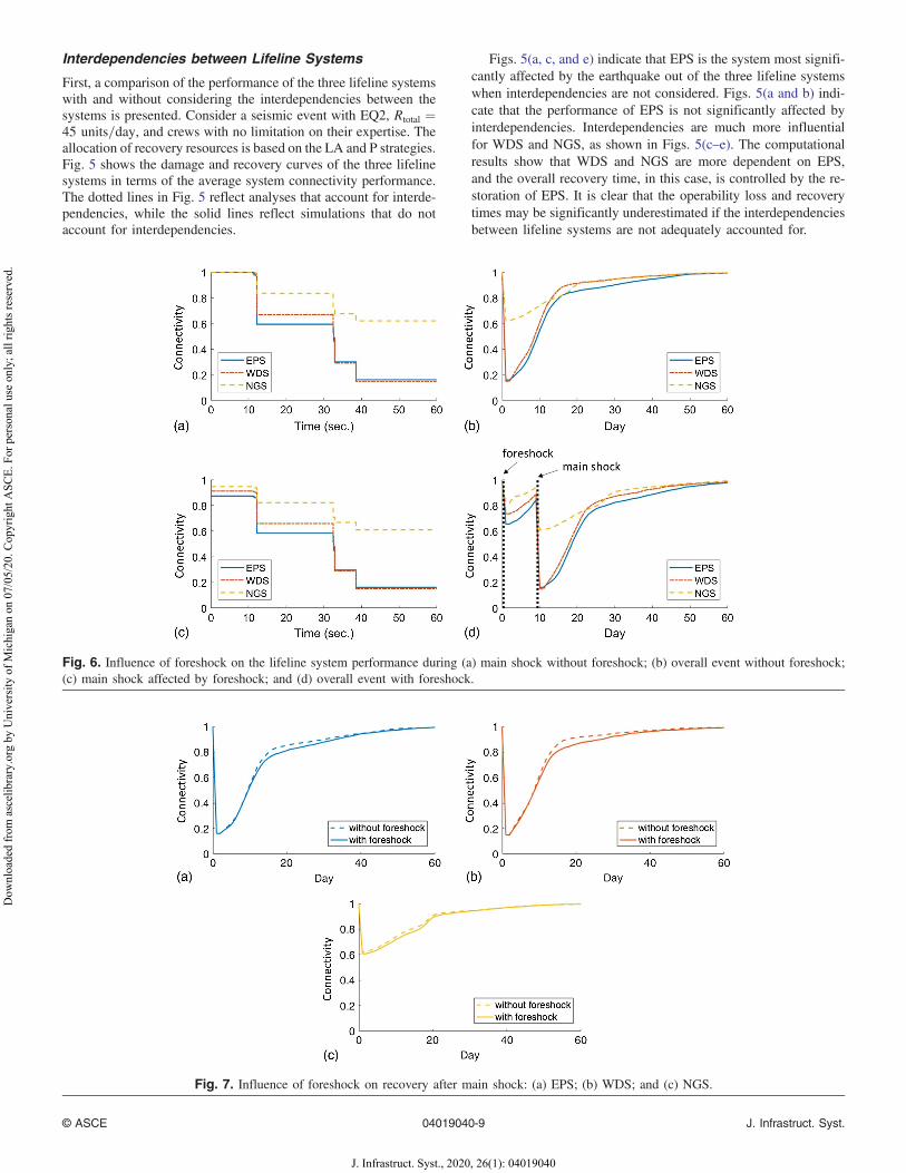
Influence of Foreshock

The influence of the foreshock is evaluated by considering a se-quence of seismic events comprised of EQ1 followed by EQ2,Rtotal ¼ 45 units=day, and crews with no limitation on their exper-tise. The allocation of the recovery resources is based on the LA andP strategies. The performance of the lifeline systems is indicated bythe connectivity ratio, as plotted in Fig. 6. Figs. 6(a and b) pertainonly to the main shock, while Figs. 6(c and d) illustrate the out-comes of EQ1 (the foreshock) leading up to EQ2 (the main shock).Figs. 6(a and c) indicate that the worst connectivity ratio of the life-line systems is governed by the main shock, which is larger than theforeshock. However, the damage inflicted by the foreshock makesthe lifeline systems more vulnerable to the later quake. As shown inFig. 7, the recovery slows down slightly in the long-term when theforeshock is considered, because the final damage after the mainshock is more severe and there are more damaged componentsin need of repair, which might not be fully reflected in the connec-tivity loss.

Influence of Aftershock

Consider a seismic event with EQ2 (main shock) followed by EQ1(aftershock), Rtotal ¼ 45 units=day, and crews with no limitation ontheir expertise. The allocation of recovery resources is based on theLA and P strategies. Fig. 8 shows the changes in system perfor-mance with an aftershock compared to EQ1 by itself. As shownin Figs. 8(a and b), the aftershock induces additional damageand decelerates the speed of restoration despite being smaller thanthe main shock. Moreover, by comparing Figs. 8(a and b) withFigs. 8(c and d), it can be seen that the damage due to the aftershockis much more serious than the damage due to a single earthquakewith the same magnitude. For example, in Fig. 8(d), the remainingconnectivity of EPS in the case with EQ1 by itself is about 0.64, butin the case with the aftershock, the connectivity of EPS after EQ1(aftershock) decreases to 0.42, as shown in Fig. 8(b).

Effect of Recovery Strategies

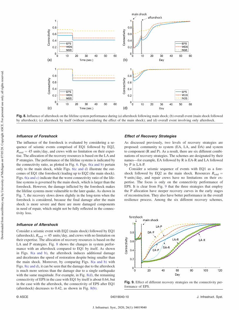
As discussed previously, two levels of recovery strategies areproposed: community to system (EA, LA, and DA) and systemto component (R and P). As a result, there are six different combi-nations of recovery strategies. The schemes are designated by theirnames—for example, EA followed by R is EA-R and LA followedby P is LA-P.

Consider a seismic sequence of events with EQ1 as a fore-shock followed by EQ2 as the main shock. Resources Rtotal ¼9 units=day, and repair crews have no limitations on their ex-pertise. The focus is only on the connectivity performance ofEPS. It is clear from Fig. 9 that the three strategies that employthe P allocation have steeper recovery curves in the early stagesof reconstruction. They also have better performance in the overallresilience process. Among the six different recovery schemes,

Fig. 8. Influence of aftershock on the lifeline system performance during (a) aftershock following main shock; (b) overall event (main shock followedby aftershock); (c) aftershock by itself (without considering the effect of the main shock); and (d) overall event involving only aftershock.

Fig. 9. Effect of different recovery strategies on the connectivity per-formance of EPS.

© ASCE 04019040-10 J. Infrastruct. Syst.

J. Infrastruct. Syst., 2020, 26(1): 04019040

Dow

nloa

ded

from

asc

elib

rary

.org

by

Uni

vers

ity o

f Mic

higa

n on

07/

05/2

0. C

opyr

ight

ASC

E. F

or p

erso

nal u

se o

nly;

all

right

s res

erve

d.

the EA-R scheme has the worst recovery performance. The bestis DA-P.

Effect of Amount and Type of Recovery Resources

To study the effect of the amount of recovery resources, consideragain a case with EQ1 as a foreshock followed by EQ2 as themain shock. In this case Rtotal varies and equals 9, 15, 30, or45 units=day, and crews have no limitation on their expertise.Focusing again on EPS, the best (DA-P) and worst (EA-R) strat-egies discussed previously are employed to maximize the contrastbetween them, and the results are shown in Figs. 10(a and b), re-spectively. As expected, recovery performance improves as morerecovery resources are allocated. Fig. 10 also shows that the effectof limited resources is significantly more pronounced in the lower-efficiency scheme. Fig. 11 compares the effect of the amount ofresources on recovery when different strategies are employed.

Again, the less efficient schemes suffer more pronounced effectswhen fewer resources are available.

Consider a similar study with crews that have specific (notgeneral) expertise—for example, a crew is only able to service aparticular lifeline system. Consider a seismic sequence of eventswith EQ1 as a foreshock, followed by EQ2 as the main shock. TheDA-P strategy is applied, and two different recovery resource con-straints are considered. First, funding is available to pay up to 15repair crews per day, that is, RtotalðtÞ ≤ 15 units=day (Constraint 1).Second, the crews are specialized, with up to five crews spe-cializing in each lifeline system, that is, RkðtÞ ≤ Rmax;k ¼ 5(Constraint 2), where RkðtÞ is the amount of recovery resourcesallocated to the kth system. Fig. 12 compares the performance ofEPS with different levels of recovery resource constraints. The fig-ure shows that the resilience of the community is overestimated ifcrew expertise is not account for, especially in the period between25 and 60 days.

Fig. 10. Effect of recovery resources on EPS with recovery strategy: (a) DA-P; and (b) EA-R.

Fig. 11. The connectivity performance of EPS adopting different recovery strategies with different recovery resources with (a) 45; (b) 30; (c) 15; and(d) 9 units=day.

© ASCE 04019040-11 J. Infrastruct. Syst.

J. Infrastruct. Syst., 2020, 26(1): 04019040

Dow

nloa

ded

from

asc

elib

rary

.org

by

Uni

vers

ity o

f Mic

higa

n on

07/

05/2

0. C

opyr

ight

ASC

E. F

or p

erso

nal u

se o

nly;

all

right

s res

erve

d.

Summary and Conclusions

A distributed computational framework was employed to model theinteractions that occur between lifeline systems during earthquakes.Various systems were modeled using simulators with disparatetemporal and spatial scales. The simulators were connected througha computational platform. Shelby County, Tennessee, was used as acase study for demonstrating the ability of the framework to modelthe interactions between three lifeline systems. The effects of differ-ent recovery strategies on system performance were examinedas the hazard unfolded and as the recovery process took place.The computational results quantified the influence of the interde-pendencies between the lifeline systems on the resilience of thecommunity.

Aside from the need to account for multiscale interdependen-cies, the case study pointed out the necessity of time-varying analy-sis as the hazard unfolded and during the recovery process. Theseismic hazard considered in this work occurred in just a fewseconds. Nevertheless, modeling the interactions that occurred be-tween the lifeline systems during the event provided insights intohow interdependencies among infrastructure systems propagateand provided clues as to how to improve their resilience. The abilityto handle differences in temporal scales between a hazard andthe recovery process is one of the key advantages of the analysis,as evinced by its ability to handle aftershocks that interact with anongoing recovery effort.

The case study showed that not taking system interdependenciesinto account will underestimate operability loss and recovery time.It was also shown that that, within the constraints of this research,the strategy of recovery resource allocation had a great impact oncommunity resilience. The impact was exacerbated when resourceswere insufficient. Among the six resource allocation strategiesstudied, the ones that adjusted based on damage/reconstructionstates enhanced resilience. This points to the necessity of maximiz-ing a community’s ability to have good information flow after adisaster. In other words, the hardening of monitoring and commu-nications systems and making them more damage-tolerant is aneffective way to increase community resilience. This, of course,can only be achieved by building, prior to the event, institutionalrelationships that will foster cooperation between the various publicand private players that would be involved in response, restoration,and recovery.

A limitation of this work lies in some of the assumptions andsimplifications made. For example, the effect of delays due to bad

weather conditions and traffic blockages or the effect of limitedconstruction materials on the available number of resource unitswas not considered. Although these omissions and simplificationsmay influence the specific results presented in this paper, the frame-work’s flexibility and extensibility permit it to address them in thefuture through the addition of new simulators or the modification ofthe existing simulators.

Data Availability Statement

All data, models, and code generated or used during the studyappear in the published article.

Acknowledgments

This work was supported by the University of Michigan andthe US National Science Foundation (NSF) through GrantNo. ACI-1638186. Any opinions, findings, conclusions, and re-commendations expressed in this paper are those of the authorsand do not necessarily reflect the views of the sponsors.

References

Adachi, T., and B. R. Ellingwood. 2008. “Serviceability of earthquake-damaged water systems: Effects of electrical power availability andpower backup systems on system vulnerability.” Reliab. Eng. Syst. Saf.93 (1): 78–88. https://doi.org/10.1016/j.ress.2006.10.014.

Adachi, T., and B. R. Ellingwood. 2009. “Serviceability assessment of amunicipal water system under spatially correlated seismic intensities.”Comput. Aided Civ. Infrastruct. Eng. 24 (4): 237–248. https://doi.org/10.1111/j.1467-8667.2008.00583.x.

Albert, R., I. Albert, and G. L. Nakarado. 2004. “Structural vulnerability ofthe North American power grid.” Phys. Rev. E 69 (2): 025103. https://doi.org/10.1103/PhysRevE.69.025103.

Atkinson, G. M., and D. M. Boore. 1995. “Ground-motion relations foreastern North America.” Bull. Seismol. Soc. Am. 85 (1): 17–30.

Barton, D. C., E. D. Eidson, D. A. Schoenwald, K. L. Stamber, and R. K.Reinert. 2000. Aspen-EE: An agent-based model of infrastructure inter-dependency. SAND2000-2925. Albuquerque, NM: Sandia NationalLaboratories.

Chang, S. E., and S. B. Miles. 2004. “The dynamics of recovery: A frame-work.” In Modeling spatial and economic impacts of disasters,edited by Y. Okuyama and S. E. Chang, 181–204. Berlin: Springer.

Chang, S. E., H. A. Seligson, and R. T. Eguchi. 1996. Estimation of theeconomic impact of multiple lifeline disruption: Memphis light, gas andwater division case study. Buffalo, NY: National Center for EarthquakeEngineering Research.

Cimellaro, G. P., C. Renschler, A. M. Reinhorn, and L. Arendt.2016. “PEOPLES: A framework for evaluating resilience.” J. Struct.Eng. 142 (10): 4016063. https://doi.org/10.1061/(ASCE)ST.1943-541X.0001514.

Cutler, H., M. Shields, D. Tavani, and S. Zahran. 2016. “Integratingengineering outputs from natural disaster models into a dynamicspatial computable general equilibrium model of Centerville.” Sustain-able Resilient Infrastruct. 1 (3–4): 169–187. https://doi.org/10.1080/23789689.2016.1254996.

Cutter, S. L., B. J. Boruff, and W. L. Shirley. 2003. “Social vulnerability toenvironmental hazards.” Social Sci. Q. 84 (2): 242–261. https://doi.org/10.1111/1540-6237.8402002.

Dudenhoeffer, D. D., M. R. Permann, and M. Manic. 2006. “CIMS: AFramework for Infrastructure InterdependencyModeling and Analysis.”In Proc., 2006 Winter Simulation Conf., 478–485. Piscataway, NJ:IEEE Press.

Duenas-Osorio, L., J. I. Craig, and B. J. Goodno. 2007. “Seismic responseof critical interdependent networks.” Earthquake Eng. Struct. Dyn.36 (2): 285–306. https://doi.org/10.1002/eqe.626.

Fig. 12. Comparison of different levels of recovery resourceconstraints.

© ASCE 04019040-12 J. Infrastruct. Syst.

J. Infrastruct. Syst., 2020, 26(1): 04019040

Dow

nloa

ded

from

asc

elib

rary

.org

by

Uni

vers

ity o

f Mic

higa

n on

07/

05/2

0. C

opyr

ight

ASC

E. F

or p

erso

nal u

se o

nly;

all

right

s res

erve

d.

Ellingwood, B. R., H. Cutler, P. Gardoni, W. G. Peacock, J. W. van deLindt, and N. Wang. 2016. “The Centerville virtual community: A fullyintegrated decision model of interacting physical and social infrastruc-ture systems.” Sustainable Resilient Infrastruct. 1 (3–4): 95–107.https://doi.org/10.1080/23789689.2016.1255000.

Eusgeld, I., D. Henzi, and W. Kröger. 2008. “Comparative evaluation ofmodeling and simulation techniques for interdependent critical infra-structures.” In Laboratory for safety analysis. Zurich, Switzerland:ETH Zurich.

FEMA. 2003. Earthquake loss estimation methodology: Technical manual.Washington, DC: National Institute of Building for the FederalEmergency Management Agency.

Ghosn, M., et al. 2016. “Performance indicators for structural systems andinfrastructure networks.” J. Aerosp. Eng. 29 (4): F4016003. https://doi.org/10.1061/(ASCE)ST.1943-541X.0001542.

González, A. D., L. Duenas-Osorio, M. Sánchez-Silva, and A. L. Medaglia.2016. “The interdependent network design problem for optimal infra-structure system restoration.” Comput. Aided Civ. Infrastruct. Eng.31 (5): 334–350. https://doi.org/10.1111/mice.12171.

Guidotti, R., H. Chmielewski, V. Unnikrishnan, P. Gardoni, T. McAllister,and J. van de Lindt. 2016. “Modeling the resilience of critical infra-structure: The role of network dependencies.” Sustainable ResilientInfrastruct. 1 (3–4): 153–168. https://doi.org/10.1080/23789689.2016.1254999.

Hernandez-Fajardo, I., and L. Duenas-Osorio. 2013. “Probabilistic study ofcascading failures in complex interdependent lifeline systems.” Reliab.Eng. Syst. Saf. 111 (Mar): 260–272. https://doi.org/10.1016/j.ress.2012.10.012.

Koliou, M., J. W. van de Lindt, T. P. McAllister, B. R. Ellingwood,M. Dillard, and H. Cutler. 2018. “State of the research in communityresilience: Progress and challenges.” Sustainable Resilient Infrastruct.1–21. https://doi.org/10.1080/23789689.2017.1418547.

Lin, P., and N. Wang. 2016. “Building portfolio fragility functions tosupport scalable community resilience assessment.” Sustainable Resil-ient Infrastruct. 1 (3–4): 108–122. https://doi.org/10.1080/23789689.2016.1254997.

Lin, S.-Y., W.-C. Chuang, L. Xu, S. El-Tawil, S. M. J. Spence, V. R. Kamat,C. C. Menassa, and J. McCormick. 2019. “A framework for modelinginterdependent effects in natural disasters: Application to wind engi-neering.” J. Struct. Eng. 145 (5): 04019025. https://doi.org/10.1061/(ASCE)ST.1943-541X.0002310.

Loggins, R., R. G. Little, J. Mitchell, T. Sharkey, and W. A. Wallace. 2019.“CRISIS: Modeling the restoration of interdependent civil and socialinfrastructure systems following an extreme event.” Nat. HazardsRev. 20 (3): 04019004. https://doi.org/10.1061/(ASCE)NH.1527-6996.0000326.

Miles, S. B., and S. E. Chang. 2007. A simulation model of urban disasterrecovery and resilience: Implementation for the 1994 Northridge earth-quake. Technical Rep. No. MCEER-07-0014. Buffalo, NY: Multidisci-plinary Center for Earthquake Engineering Research.

Miles, S. B., and S. E. Chang. 2011. “ResilUS: A community based disasterresilience model.” Cartography Geographic Inf. Sci. 38 (1): 36–51.https://doi.org/10.1559/1523040638136.

Moreno, J., and D. Shaw. 2019. “Community resilience to power outagesafter disaster: A case study of the 2010 Chile earthquake and tsunami.”Int. J. Disaster Risk Reduct. 34 (1): 448–458. https://doi.org/10.1016/j.ijdrr.2018.12.016.

Morshedlou, N., A. D. González, and K. Barker. 2018. “Work crew routingproblem for infrastructure network restoration.” Transp. Res. Part B118 (Dec): 66–89. https://doi.org/10.1016/j.trb.2018.10.001.

NER (National Earthquake Resilience). 2011. National earthquakeresilience: Research, implementation, and outreach. Washington,DC: National Academies Press.

Ouyang, M. 2014. “Review on modeling and simulation of interdependentcritical infrastructure systems.” Reliab. Eng. Syst. Saf. 121 (Jan): 43–60.https://doi.org/10.1016/j.ress.2013.06.040.

PEER (Pacific Earthquake Engineering Research Center). 2018. “PEERground motion database.” Accessed January, 2018. https://ngawest2.berkeley.edu/.

Reilly, A. C., S. D. Guikema, L. Zhu, and T. Igusa. 2017. “Evolution ofvulnerability of communities facing repeated hazards.” PLoS One12 (9): e0182719. https://doi.org/10.1371/journal.pone.0182719.

Renschler, C. S., A. E. Frazier, L. A. Arendt, G. P. Cimellaro, A. M.Reinhorn, and M. Bruneau. 2010. “Developing the ‘PEOPLES’ resil-ience framework for defining and measuring disaster resilience at thecommunity scale.” In Proc., 9th US National and 10th Canadian Conf.on Earthquake Engineering (9USN/10CCEE). Oakland, CA: Earth-quake Engineering Research Institute.

Rinaldi, S. M., J. P. Peerenboom, and T. K. Kelly. 2001. “Identifying,understanding, and analyzing critical infrastructure interdependencies.”IEEE Control Syst. 21 (6): 11–25. https://doi.org/10.1109/37.969131.

Schmeltz, M. T., S. K. González, L. Fuentes, A. Kwan, A. Ortega-Williams,and L. P. Cowan. 2013. “Lessons from hurricane sandy: A communityresponse in Brooklyn, New York.” J. Urban Health 90 (5): 799–809.https://doi.org/10.1007/s11524-013-9832-9.

Schoenwald, D. A., D. C. Barton, and M. A. Ehlen. 2004. “An agent-basedsimulation laboratory for economics and infrastructure interdepend-ency.” In Vol. 1292 of Proc., 2004 American Control Conf.,1295–1300. Piscataway, NJ: IEEE Press.

Shinozuka, M., X. Dong, J. Xianhe, and T. C. Cheng. 2005. “Seismicperformance analysis for the LADWP power system.” In Proc.,2005 IEEE=PES Transmission and Distribution Conf. and Exposition:Asia and Pacific, 1–6. Piscataway, NJ: IEEE Press.

Song, J., and S.-Y. Ok. 2010. “Multi-scale system reliability analysis oflifeline networks under earthquake hazards.” Earthquake Eng. Struct.Dyn. 39 (3): 259–279. https://doi.org/10.1002/eqe.938.

USGS. 2018. “Memphis, Shelby County seismic hazard maps and data.”Accessed February, 2018. https://earthquake.usgs.gov/hazards/urban/memphis/grid_download.php.

Zhang, P., and S. Peeta. 2011. “A generalized modeling framework toanalyze interdependencies among infrastructure systems.” Transp. Res.Part B: Methodol. 45 (3): 553–579. https://doi.org/10.1016/j.trb.2010.10.001.

Zimmerman, R. 2001. “Social Implications of Infrastructure networkInteractions.” J. Urban Technol. 8 (3): 97–119. https://doi.org/10.1080/106307301753430764.

© ASCE 04019040-13 J. Infrastruct. Syst.

J. Infrastruct. Syst., 2020, 26(1): 04019040

Dow

nloa

ded

from

asc

elib

rary

.org

by

Uni

vers

ity o

f Mic

higa

n on

07/

05/2

0. C

opyr

ight

ASC

E. F

or p

erso

nal u

se o

nly;

all

right

s res

erve

d.