Time-dependent density-functional theory in the projector augmented-wave method

Time-dependent density-functional theory in the projectoraugmented-wave method

Michael Walter,1,a� Hannu Häkkinen,1,2 Lauri Lehtovaara,3 Martti Puska,3 Jussi Enkovaara,4

Carsten Rostgaard,5 and Jens Jørgen Mortensen5

1Department of Physics, Nanoscience Center, University of Jyväskylä, FIN-40014 Jyväskylä, Finland2Department of Chemistry, Nanoscience Center, University of Jyväskylä, FIN-40014, Jyväskylä, Finland3Department of Engineering Physics, Helsinki University of Technology, P.O. Box 1100,FIN-02015 TKK, Finland4CSC Scientific Computing Ltd., FI-02101 Espoo, Finland5CAMd, Department of Physics, Technical University of Denmark, DK-2800 Lyngby, Denmark

�Received 9 April 2008; accepted 19 May 2008; published online 23 June 2008�

We present the implementation of the time-dependent density-functional theory both inlinear-response and in time-propagation formalisms using the projector augmented-wave method inreal-space grids. The two technically very different methods are compared in the linear-responseregime where we found perfect agreement in the calculated photoabsorption spectra. We discuss thestrengths and weaknesses of the two methods as well as their convergence properties. Wedemonstrate different applications of the methods by calculating excitation energies and excitedstate Born–Oppenheimer potential surfaces for a set of atoms and molecules with thelinear-response method and by calculating nonlinear emission spectra using the time-propagationmethod. © 2008 American Institute of Physics. �DOI: 10.1063/1.2943138�

I. INTRODUCTION

The density-functional theory1,2 �DFT� has been verysuccessful for ground-state calculations of molecular andcondensed-matter systems due to its favorable balance ofcost against accuracy. Properties such as ground-state totalenergies, lattice constants, and equilibrium geometries arenowadays calculated routinely for systems containing up to afew hundred atoms. However, there are several scientificallyand technologically interesting quantities which are relatedto excited states of the system and are thus beyond the realmof the standard DFT. In recent years, the time-dependentDFT �TDDFT� �Ref. 3� has become a popular tool for calcu-lating excited-state properties such as linear and nonlinearoptical responses.4–9

The most general realization of the TDDFT is the time-propagation scheme5 in which the time-dependent Kohn–Sham �KS� equations are integrated over the time domain. Inthe linear-response regime the excitation energies can also becalculated in the frequency space by solving a matrix equa-tion in a particle-hole basis.4 This is the so-called linear-response scheme. The time-propagation and the linear-response scheme are complementary as they have differentadvantages and disadvantages. For example, the linear-response scheme provides all the excitations in a single cal-culation, while the time-propagation provides only the exci-tations corresponding to the given initial perturbation andseveral separate calculations may be needed. On the otherhand, the time-propagation has a wider applicability as alsonon-linear-response phenomena, such as the high-harmonicsgeneration in intense laser beams and general time-

dependent phenomena, in which for example the ionic struc-ture relaxes as a function of time, can be studied. Computa-tionally, the time-propagation scales more favorably with thesystem size than the linear-response scheme. However, theprefactor in time-propagation is larger, so that the cross-overin efficiency is reached at relatively large systems.

Previously, there have been several implementations ofthe linear-response and the time-propagation formalisms us-ing a variety of methods such as localized basis sets,10,11

plane waves,12–15 and real-space grids.5,16,17 The plane-waveand the real-space implementations have used the pseudopo-tential approximation which has been either of the norm-conserving or ultrasoft flavor. To our knowledge, the projec-tor augmented-wave �PAW� method18 has not been used intime-dependent density-functional calculations previously.Here, we present implementation of both time-propagationand linear-response TDDFT in the electronic-structure pro-gram GPAW,19,20 which uses the PAW method and uniformreal-space grids.

The real-space PAW method has several advantages bothin ground-state and in time-dependent calculations. First,there is a single convergence parameter, the grid spacing,which controls the accuracy of the discretization. Differentboundary conditions can be handled easily and especially theability to treat finite systems without supercells is importantfor TDDFT. The PAW method can be applied on the samefooting to all elements, for example, it provides a reliabledescription of the transition metal elements and the first rowelements with open p-shells. These are often problematic forstandard pseudopotentials. Also, the PAW method reducesthe number of grid points required for accurate calculationsin comparison with pseudopotential calculations. Thus, thedimension of the Hamiltonian matrix is reduced and one isa�Electronic mail: [email protected].

THE JOURNAL OF CHEMICAL PHYSICS 128, 244101 �2008�

0021-9606/2008/128�24�/244101/10/$23.00 © 2008 American Institute of Physics128, 244101-1

Downloaded 21 Jun 2010 to 192.38.67.112. Redistribution subject to AIP license or copyright; see http://jcp.aip.org/jcp/copyright.jsp

also allowed to use longer time steps in time-propagation.15

Finally, the real-space formalism allows efficient paralleliza-tion with domain-decomposition techniques.

The present paper is organized as follows. In Sec. II Awe present the basic features of the PAW method. The linear-response formulation of the TDDFT within the PAW methodis presented in Sec. II B and the time-propagation scheme isreviewed in Sec. II C. In Sec. III we show that the two meth-ods give identical results in the linear-response regime bycalculating the optical absorption spectra for the Na2 andC6H6 molecules. Next, we focus on the linear-responsescheme and calculate excitation energies for a set of divalentatoms followed by Born–Oppenheimer potentials of excitedstates of Na2. The applicability of the time-propagation in thenonlinear regime is demonstrated by calculating emissionspectra of the Be atom in strong laser fields. The conver-gence properties of the two methods are discussed in Sec. IV.Finally, we give a brief summary in Sec. V.

II. THEORY

A. Ground state

The implementation of the PAW method using a real-space grid is explained in detail in Ref. 19. We will give herejust a short introduction with the main purpose of definingthe quantities needed for the time-propagation and linear-response calculation. In the PAW method, a true all-electronKS wave function �n can be obtained through a linear trans-

formation from a smooth pseudo-wave-function �n via

�n�r� = T�n, �1�

where n denotes a combined band and spin index. Using the

explicit representation of T, the KS wave functions can beexpressed as

�n�r� = �n�r� + �a

��na�r − Ra� − �n

a�r − Ra�� , �2�

where �na and �n

a are the all-electron and smooth continua-tions of �n inside the augmentation region of the atom a atposition Ra, respectively. Their difference vanishes by defi-

nition outside the augmentation region. �na and �n

a may beexpanded in terms of atom-centered all-electron wave func-tions �a and their smooth counterparts �a, respectively, i.e.,

�na�r� = �

j

Pnja � j

a�r�, �na�r� = �

j

Pnja � j

a�r� , �3�

with the same coefficients Pnja = �pj ��n�, where the pj are the

so called projector functions.18,19 The main quantity of DFT,the electron density n�r� has a similar partitioning as thewave functions �this behavior can be shown to be true for allquantities that can be expressed as expectation values of lo-cal operators18�. Thus,

n�r� = n�r� + �a

�na�r − Ra� − na�r − Ra�� , �4�

where the all-electron density inside the augmentation region

na�r� = �i1i2

Di1i2a �i1

a �r��i2a �r� �5�

and its smooth counterpart

na�r� = �i1i2

Di1i2a �i1

a �r��i2a �r� �6�

appear. Denoting the ground-state occupation numbers by fn,the above atomic density matrix can be expressed as19

Di1i2a = �

n

Pni1

a* fnPni2a . �7�

B. Linear response

In the following we discuss the linear-response theory inthe TDDFT from a practical view, rather than from its formalderivation which can be found in the original references4,10,21

or in more recent work.22 We follow closely the notationused by Casida,4 who showed that in the linear-response TD-DFT the calculation of excitation energies can be reduced tosolving the eigenvalue equation of the following form:

�FI = �I2FI, �8�

where ��I is the transition energy from the ground state tothe excited state I. Expanding the matrix � in KS singleparticle-hole excitations leads to

�ij�,kq� = �ik� jq���ij�2 + 2f ij�ij�fkq�kq�Kij�,kq�, �9�

where ij�= j�−i� are the energy differences and f ij�= f i�

− f j� are the occupation number differences of the KS states.The indices i, j, k, and q are band indices, whereas � and �denote spin projection indices. The coupling matrix can besplit into two parts Kij�,kq�=Kij�,kq�

RPA +Kij�,kq�xc . The former is

the so-called random phase approximation �RPA� part,

Kij�,kq�RPA = dr1dr2

nij�* �r1�nkq��r2�

�r1 − r2�¬ �nij��nkq�� , �10�

where nij� is the i , j density matrix element or pair densitycorresponding to the spin �. Kij�,kq�

RPA describes the effect ofthe linear density response via the classical Hartree energy.The second is the exchange-correlation part,

Kij�,kq�xc = dr1dr2n

ij�* �r1�

�2Exc

���r1����r2�nkq��r2� , �11�

where � is the spin density. Kij�,kq�xc describes the effect of

the linear density response via the exchange and correlationenergy.

We discuss the forms of the coupling matrix for the twoparts separately and suppress the explicit dependence on thespin projection unless it is explicitly needed. In both parts ofthe coupling matrix the pair density nij�r�=�

i*�r�� j�r� ap-

pears. This quantity can be partitioned in the same way as theelectron density, i.e.,

nij = nij + �a

�nija − nij

a � , �12�

where we have dropped the dependence on the position forbrevity. Inserting this expression directly into the integral in

244101-2 Walter et al. J. Chem. Phys. 128, 244101 �2008�

Downloaded 21 Jun 2010 to 192.38.67.112. Redistribution subject to AIP license or copyright; see http://jcp.aip.org/jcp/copyright.jsp

Eq. �10� would lead to overlaps of different augmentationspheres due to the nonlocality of the Coulomb operator �r1

−r2�−1. These overlaps have to be avoided. The same prob-lem appears already in the calculations of the Hartree energyin the ground-state problem.18,19 It can be solved by intro-

ducing compensation charge densities Zija , defined to fulfill

dr2nij

a �r2� − nija �r2� − Zij

a �r2��r1 − r2�

= 0, �13�

for �r1−Ra��rca, i.e., outside the augmentation sphere. The

compensation charge densities can be expanded in terms ofspherical harmonics YL,18,19

Zija �r� = �

L

QL,ija gl

a�r�YL�r� , �14�

where L stands for the combined values of angular momen-tum quantum numbers l and m. The choice of local functionsgl

a�r� is arbitrary as long as they fulfill

drrl+2gla�r� = 1, �15�

and they are sufficiently localized inside the augmentationsphere. For the particular choice of gl

a�r� in our calculations

we refer to Eq. �B1� in Ref. 19. Due to Eq. �13� the coeffi-cients QL,ij

a have to be

QL,ij = �i1i2

�L,i1i2Pii1

a Pji2a , �16�

with the constants

�L,i1i2= drrlYL�r���i1

a �r��i2a �r� − �i1

a �r��i2a �r�� . �17�

Using the shorthand

ij�r� ª nij�r� + �a

Zija �r − Ra� , �18�

we may write the RPA part of the kernel in the followingform:

Kij,kqRPA = �ij�kq� + �

a

�Kij,kqRPA,a, �19�

which has the desired partitioning in a pure smooth part�ij � kq� and local corrections �Kij�,kq�

RPA,a inside the augmenta-tion spheres. The explicit form of these corrections is givenin Appendix A �Eq. �A3��.

The exchange-correlation part of the coupling matrix isevaluated in a finite-difference scheme23,24 as

Kij�,kq�xc �n�,n�� = lim

→0 drn

ij�* �r�

vxc� �n�,n� + nkq���r� − vxc

� �n�,n� − nkq���r�2

, �20�

where we denote that Kij�,kq�xc is a functional of the spin den-

sities explicitly. The finite-difference scheme is quite insen-sitive to the actual numerical value for as will be shown inSec. III. For the local density approximation �LDA� and thegeneralized gradient approximation for the electron ex-change and correlation we can write

Kij�,kq�xc �n�,n�� = Kij�,kq�

xc �n�, n�� + �a

�Kij�,kq�xc,a , �21�

where Kij�,kq�xc depends on the smooth densities and the cor-

rections �Kij�,kq�xc,a are localized inside the atomic augmenta-

tion spheres. The explicit form of these corrections is givenin Appendix B �Eq. �B1��.

In optical absorption spectra not only the excitation en-ergies but also the corresponding dipole oscillator strengthsare of interest. They are dimensionless and can be written as

f I =2me

�e2 �I�I 2 , �22�

where me is the electron mass, e is the unit charge, and =x ,y ,z denotes the direction of the light polarization. Thedipole transition moment,

�I = − e�0��k=1

N

rk�I� , �23�

is defined through the many-particle ground and excitedstates �0� and �I�, respectively. Above, N is the number ofelectrons with their coordinates rk, k=1, . . . ,N. In linear-response TDDFT the oscillator strength for a transition I canbe obtained using the corresponding eigenvector FI of the �matrix and the KS transition dipoles,

�ij� = − e��i��r�� j�� , �24�

between the KS states �i� and � j�. The oscillator strengthsare evaluated then as4

f I =2me

�e2 � �ij�

f i��f j�

��ij�� f ij�ij��FI�ij��2

. �25�

In PAW the KS transition dipoles can be partitioned as

�ij� = − e��i��r�� j�� + �a

�pq

Pi�p* Pj�q�pq

a , �26�

where the local corrections are

244101-3 Projector augmented-wave method J. Chem. Phys. 128, 244101 �2008�

Downloaded 21 Jun 2010 to 192.38.67.112. Redistribution subject to AIP license or copyright; see http://jcp.aip.org/jcp/copyright.jsp

��pqa �m = − e4���1m,pq

a

3+ �L=0,pq

a �Ra�m , �27�

with the constants �L,pqa defined in Eq. �17�.

C. Time-propagation

The scheme for propagating time-dependent KS wavefunctions within the ultrasoft pseudopotential or projectoraugmented-wave method was already described by Qianet al.14 As our implementation follows closely theirs, it isreviewed only briefly here.

The all-electron time-dependent Schrödinger-type KS

equation with the Hamiltonian H�t�, i.e.,

i��

�t�n�t� = H�t��n�t� , �28�

is transformed to the PAW formalism as follows. First theall-electron wave function is replaced by the projector opera-

tor operating on the pseudo-wave-function �n= T�n. Then

Eq. �28� is operated from the left by the adjoint operator T†,i.e.,

i�T† �

�tT�n�t� = T†H�t�T�n�t� . �29�

If the projector operator T is independent of time, i.e., thenuclei do not move, the above equation reads as

i�S�

�t�n�t� = H�t��n�t� , �30�

where S= T†T is the PAW overlap operator and H�t�= T†H�t�T is the time-dependent PAW Hamiltonian includingthe external time-dependent potential.

The linear absorption spectrum is obtained in the time-propagation scheme by applying a very weak delta-functionpulse of a dipole field,5

E�t� = �ko��t��

a0e, �31�

to the system and then following the time-evolution of thedipole vector ��t�. Above, � is a unitless perturbationstrength parameter, ko is a unit vector giving the polarizationdirection of the field, and a0 is the Bohr radius. The deltapulse excites all possible frequencies at time zero, so that theKS wave functions change instantaneously to

��t = 0+� = exp�i�

a0ko · r���t = 0−� . �32�

Then the system is let to evolve freely.To see the connection to the linear-response calculations,

we study the effect of the delta kick in the many-body pic-ture. If the pulse strength is weak, i.e., ��1, the time-dependent many-body wave function after the kick is

���t = 0+�� = �1 − i�

ea0ko · ���0� + O��2� , �33�

where �=−e�k=1N rk is the dipole operator. When the system

evolves freely it can be expanded in eigenstates �0� and �I� ofthe unperturbed Hamiltonian as

���t�� = c0�0� + �I

e−i�ItcI�I� , �34�

with the coefficients

c0 = 1 − i�

ea0ko · �0���0� , �35�

and

cI = − i�

ea0ko · �I���0� . �36�

The time-dependent density can be written as25

n�r,t� = n0�r� + �I

�e−i�ItcI�0�n�r��I� + c.c.� , �37�

where n=�k=1N ��r−rk� denotes the density operator. In the

absence of magnetic fields all states can be chosen to be realresulting in the time-dependent dipole moment ��t�=−e�drn�r , t�r of the following form:

��t� = ��0� −2�

ea0�

I

sin��It��ko · �I��I. �38�

From this the dipole transition moment and hence the oscil-lator strength can be extracted via the Fourier transform. Inpractice, one calculates the generalization of the oscillatorstrength, the dipole strength tensor with respect to the polar-ization direction, ko via14

S���ko =2mea0

e���

1

�

0

T

dt sin��t�g�t����0� − ��t�� , �39�

where T is the simulation time, and g�t� is an envelope func-tion being finite in the time window only. The envelope func-tion, typically a Gaussian or an exponential decay, yields theshapes of the simulated spectral lines, Gaussians and Lorent-zians, respectively, removing the effects of the finite simula-tion time. The dipole strength tensor is connected to thefolded oscillator strength via

k o · S���k

o = �I

f I g�� − �I� , �40�

where g��� is the normalized Fourier transform of g�t� andk

o is the unit vector in the direction =x ,y ,z.In addition to the linear regime, the time-propagation

can be used to interrogate the nonlinear regime of the light-matter interaction. When an atom or a molecule resides in alaser field E�t�=E0 sin��t� of frequency � electrons begin tooscillate with this frequency. If the field is strong enough,nonlinear terms in the polarizability of the atom begin tocontribute.26 As a result, integer multiples of the field fre-quency, i.e., harmonics, appear in the emission spectrum.The intensities H of the emitted frequencies can be calcu-lated from the acceleration of the dipole moment,27 i.e.,

244101-4 Walter et al. J. Chem. Phys. 128, 244101 �2008�

Downloaded 21 Jun 2010 to 192.38.67.112. Redistribution subject to AIP license or copyright; see http://jcp.aip.org/jcp/copyright.jsp

H��� � �0

T

dt exp�i�t�d2

dt2g�t����t� − ��0���2

. �41�

In the present implementation of the time-propagation,the time-dependent equations are solved using the Crank–Nicolson propagator with a predictor-corrector step28 �thischoice is not unique, for other possible propagators see Ref.29�. The predictor-corrector scheme is required to efficientlyhandle the nonlinearity in the Hamiltonian, i.e., to obtain areasonable approximation for the Hamiltonian in a futuretime. In the predictor step, the wave functions are propagatedby approximating the Hamiltonian to be constant during the

time step, i.e., H�t+�t /2�= H�t�+O��t� and then solving alinear equation for the predicted future wave functions

�npred�t+�t�,

�S + iH�t��t/2���npred�t + �t�

= �S − iH�t��t/2���n�t� + O��t2� . �42�

The Hamiltonian in the middle of the time step is approxi-mated as

H�t + �t/2� = 12 �H�t� + Hpred�t + �t�� , �43�

where Hpred�t+�t� is obtained from the predicted wave func-

tions. In the corrector step, the improved Hamiltonian H�t+�t /2� is used to obtain the final, more accurate, propagated

wave functions �n�t+�t� from

�S + iH�t + �t/2��t/2���n�t + �t�

= �S − iH�t + �t/2��t/2���n�t� + O��t3� . �44�

The matrices in the linear equations �Eqs. �42� and �44�� arecomplex symmetric �not Hermitian�, and we solve the equa-tions using the biconjugate gradient stabilized method.30

As the Crank–Nicolson propagator is valid only for ashort time step, repeated application of the propagator is re-quired in any practical simulation. Note that no further im-provement in the order of the error is obtained by repeatingthe corrector step with an improved approximation becausethe Crank–Nicolson itself is only accurate to the second or-der. Thus, in order to obtain more accurate results, it is moreefficient to reduce the time step instead of repeating the cor-recting step more than once.

III. RESULTS AND DISCUSSION

In this section we will present example calculations forthe linear-response and time-propagation schemes. The twocomputationally very different approaches are applied to thesame systems and very good agreement is found in thelinear-response regime. The strengths and weaknesses ofboth methods are discussed.

We apply consistently the LDA �Ref. 31� in all calcula-tions. Zero Dirichlet boundary conditions are used for thefinite systems studied both in the ground state as well as inthe time-propagation calculations. A grid spacing of h=0.2 Å is used for the representation of the smooth wavefunctions unless otherwise specified.

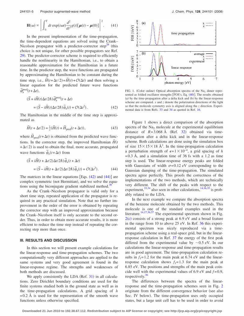
Figure 1 shows a direct comparison of the absorptionspectra of the Na2 molecule at the experimental equilibriumdistance of R=3.068 Å �Ref. 32� obtained via time-propagation after a delta kick and in the linear-responsescheme. Both calculations are done using the simulation boxof size 15�15�18 Å3. In the time-propagation calculationa perturbation strength of �=1�10−4, a grid spacing of h=0.3 Å, and a simulation time of 36 fs with a 1.2 as timestep is used. The linear-response energy peaks are foldedwith Gaussians of width �=0.12 eV corresponding to theGaussian damping of the time-propagation. The simulatedspectra agree perfectly. This proofs the correctness of theimplementations of the two methods, which are technicallyvery different. The shift of the peaks with respect to theexperiment,33,34 also seen in other calculations,14,16,35 is prob-ably related to the LDA.

In the next example we compare the absorption spectraof the benzene molecule obtained by the two methods. Thismolecule is one of the standard examples used in theliterature.14,17,36,37 The experimental spectrum shown in Fig.2�c� consists of a strong peak at 6.9 eV and a broad featurein the range from 10 to above 25 eV. In Ref. 36 this experi-mental spectrum was nicely reproduced via a time-propagation scheme using a real-space grid, but in the linear-response calculation in Ref. 37 the energy of the first peakdiffered from the experimental value by �0.5 eV. In ourcalculations the linear-response and time-propagation resultsare in good agreement. The time-propagation calculation re-sults in f I=1.2 for the main peak at 6.74 eV and the linear-response calculation shows f I=1.3 for the main peak at6.85 eV. The positions and strengths of the main peak coin-cide well with the experimental values of 6.9 eV and f =0.9,respectively.36

The differences between the spectra of the linear-response and the time-propagation schemes seen in Fig. 2originate from the different convergence behavior �see alsoSec. IV below�. The time-propagation uses only occupiedstates, but a large unit cell has to be used in order to avoid

FIG. 1. �Color online� Optical absorption spectra of the Na2 dimer repre-sented as folded oscillator strengths �FOS’s, Eq. �40��. The results obtained�a� by the time-propagation after a delta kick and �b� by the linear-responsescheme are compared. x and z denote the polarization directions of the lightso that the molecule symmetry axis is aligned along the z direction. Experi-mental data is from Refs. 33 and 34 as quoted in Ref. 16.

244101-5 Projector augmented-wave method J. Chem. Phys. 128, 244101 �2008�

Downloaded 21 Jun 2010 to 192.38.67.112. Redistribution subject to AIP license or copyright; see http://jcp.aip.org/jcp/copyright.jsp

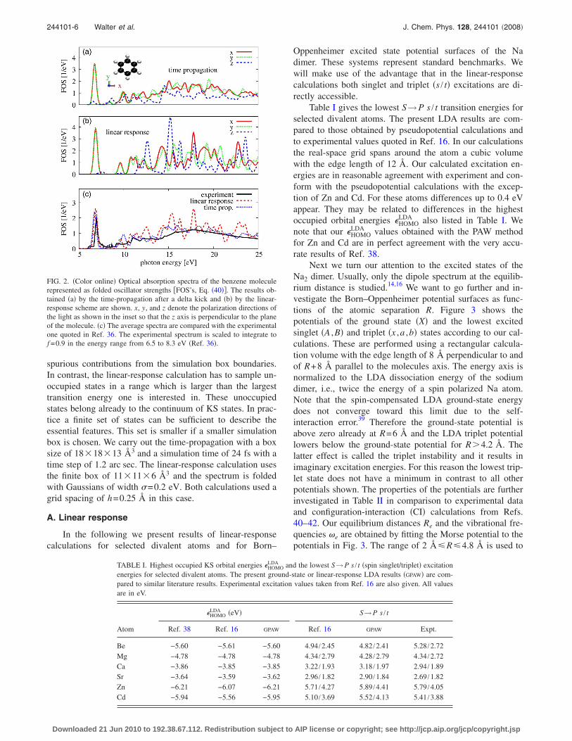
spurious contributions from the simulation box boundaries.In contrast, the linear-response calculation has to sample un-occupied states in a range which is larger than the largesttransition energy one is interested in. These unoccupiedstates belong already to the continuum of KS states. In prac-tice a finite set of states can be sufficient to describe theessential features. This set is smaller if a smaller simulationbox is chosen. We carry out the time-propagation with a boxsize of 18�18�13 Å3 and a simulation time of 24 fs with atime step of 1.2 arc sec. The linear-response calculation usesthe finite box of 11�11�6 Å3 and the spectrum is foldedwith Gaussians of width �=0.2 eV. Both calculations used agrid spacing of h=0.25 Å in this case.

A. Linear response

In the following we present results of linear-responsecalculations for selected divalent atoms and for Born–

Oppenheimer excited state potential surfaces of the Nadimer. These systems represent standard benchmarks. Wewill make use of the advantage that in the linear-responsecalculations both singlet and triplet �s / t� excitations are di-rectly accessible.

Table I gives the lowest S→P s / t transition energies forselected divalent atoms. The present LDA results are com-pared to those obtained by pseudopotential calculations andto experimental values quoted in Ref. 16. In our calculationsthe real-space grid spans around the atom a cubic volumewith the edge length of 12 Å. Our calculated excitation en-ergies are in reasonable agreement with experiment and con-form with the pseudopotential calculations with the excep-tion of Zn and Cd. For these atoms differences up to 0.4 eVappear. They may be related to differences in the highestoccupied orbital energies �HOMO

LDA also listed in Table I. Wenote that our �HOMO

LDA values obtained with the PAW methodfor Zn and Cd are in perfect agreement with the very accu-rate results of Ref. 38.

Next we turn our attention to the excited states of theNa2 dimer. Usually, only the dipole spectrum at the equilib-rium distance is studied.14,16 We want to go further and in-vestigate the Born–Oppenheimer potential surfaces as func-tions of the atomic separation R. Figure 3 shows thepotentials of the ground state �X� and the lowest excitedsinglet �A ,B� and triplet �x ,a ,b� states according to our cal-culations. These are performed using a rectangular calcula-tion volume with the edge length of 8 Å perpendicular to andof R+8 Å parallel to the molecules axis. The energy axis isnormalized to the LDA dissociation energy of the sodiumdimer, i.e., twice the energy of a spin polarized Na atom.Note that the spin-compensated LDA ground-state energydoes not converge toward this limit due to the self-interaction error.39 Therefore the ground-state potential isabove zero already at R=6 Å and the LDA triplet potentiallowers below the ground-state potential for R�4.2 Å. Thelatter effect is called the triplet instability and it results inimaginary excitation energies. For this reason the lowest trip-let state does not have a minimum in contrast to all otherpotentials shown. The properties of the potentials are furtherinvestigated in Table II in comparison to experimental dataand configuration-interaction �CI� calculations from Refs.40–42. Our equilibrium distances Re and the vibrational fre-quencies �e are obtained by fitting the Morse potential to thepotentials in Fig. 3. The range of 2 Å�R�4.8 Å is used to

FIG. 2. �Color online� Optical absorption spectra of the benzene moleculerepresented as folded oscillator strengths �FOS’s, Eq. �40��. The results ob-tained �a� by the time-propagation after a delta kick and �b� by the linear-response scheme are shown. x, y, and z denote the polarization directions ofthe light as shown in the inset so that the z axis is perpendicular to the planeof the molecule. �c� The average spectra are compared with the experimentalone quoted in Ref. 36. The experimental spectrum is scaled to integrate tof =0.9 in the energy range from 6.5 to 8.3 eV �Ref. 36�.

TABLE I. Highest occupied KS orbital energies �HOMOLDA and the lowest S→P s / t �spin singlet/triplet� excitation

energies for selected divalent atoms. The present ground-state or linear-response LDA results �GPAW� are com-pared to similar literature results. Experimental excitation values taken from Ref. 16 are also given. All valuesare in eV.

Atom

�HOMOLDA �eV� S→P s / t

Ref. 38 Ref. 16 GPAW Ref. 16 GPAW Expt.

Be −5.60 −5.61 −5.60 4.94 /2.45 4.82 /2.41 5.28 /2.72Mg −4.78 −4.78 −4.78 4.34 /2.79 4.28 /2.79 4.34 /2.72Ca −3.86 −3.85 −3.85 3.22 /1.93 3.18 /1.97 2.94 /1.89Sr −3.64 −3.59 −3.62 2.96 /1.82 2.90 /1.84 2.69 /1.82Zn −6.21 −6.07 −6.21 5.71 /4.27 5.89 /4.41 5.79 /4.05Cd −5.94 −5.56 −5.95 5.10 /3.69 5.52 /4.13 5.41 /3.88

244101-6 Walter et al. J. Chem. Phys. 128, 244101 �2008�

Downloaded 21 Jun 2010 to 192.38.67.112. Redistribution subject to AIP license or copyright; see http://jcp.aip.org/jcp/copyright.jsp

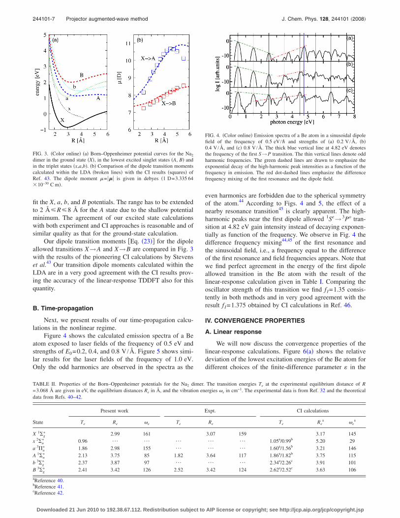
fit the X, a, b, and B potentials. The range has to be extendedto 2 �R�8 Šfor the A state due to the shallow potentialminimum. The agreement of our excited state calculationswith both experiment and CI approaches is reasonable and ofsimilar quality as that for the ground-state calculation.

Our dipole transition moments �Eq. �23�� for the dipoleallowed transitions X→A and X→B are compared in Fig. 3with the results of the pioneering CI calculations by Stevenset al.43 Our transition dipole moments calculated within theLDA are in a very good agreement with the CI results prov-ing the accuracy of the linear-response TDDFT also for thisquantity.

B. Time-propagation

Next, we present results of our time-propagation calcu-lations in the nonlinear regime.

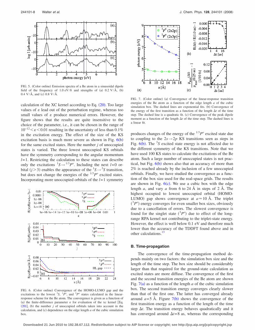
Figure 4 shows the calculated emission spectra of a Beatom exposed to laser fields of the frequency of 0.5 eV andstrengths of E0=0.2, 0.4, and 0.8 V /Å. Figure 5 shows simi-lar results for the laser fields of the frequency of 1.0 eV.Only the odd harmonics are observed in the spectra as the

even harmonics are forbidden due to the spherical symmetryof the atom.44 According to Figs. 4 and 5, the effect of anearby resonance transition45 is clearly apparent. The high-harmonic peaks near the first dipole allowed 1Se→ 3Po tran-sition at 4.82 eV gain intensity instead of decaying exponen-tially as function of the frequency. We observe in Fig. 4 thedifference frequency mixing44,45 of the first resonance andthe sinusoidal field, i.e., a frequency equal to the differenceof the first resonance and field frequencies appears. Note thatwe find perfect agreement in the energy of the first dipoleallowed transition in the Be atom with the result of thelinear-response calculation given in Table I. Comparing theoscillator strength of this transition we find f I=1.35 consis-tently in both methods and in very good agreement with theresult f I=1.375 obtained by CI calculations in Ref. 46.

IV. CONVERGENCE PROPERTIES

A. Linear response

We will now discuss the convergence properties of thelinear-response calculations. Figure 6�a� shows the relativedeviation of the lowest excitation energies of the Be atom fordifferent choices of the finite-difference parameter in the

FIG. 3. �Color online� �a� Born–Oppenheimer potential curves for the Na2

dimer in the ground state �X�, in the lowest excited singlet states �A, B� andin the triplet states �x,a,b�. �b� Comparison of the dipole transition momentscalculated within the LDA �broken lines� with the CI results �squares� ofRef. 43. The dipole moment �= ��� is given in debyes �1 D=3.335 64�10−30 C m�.

TABLE II. Properties of the Born–Oppenheimer potentials for the Na2 dimer. The transition energies Te at the experimental equilibrium distance of R=3.068 Å are given in eV, the equilibrium distances Re in Å, and the vibration energies �e in cm−1. The experimental data is from Ref. 32 and the theoreticaldata from Refs. 40–42.

State

Present work Expt. CI calculations

Te Re �e Te Re Te Rea �e

a

X 1�g+ 2.99 161 3.07 159 3.17 145

x 2�u+ 0.96 ¯ ¯ ¯ ¯ ¯ 1.05a/0.99b 5.20 29

a 3�u+ 1.86 2.98 155 ¯ ¯ ¯ 1.60a/1.56b 3.21 146

A 1�u+ 2.13 3.75 85 1.82 3.64 117 1.86a/1.82b 3.75 115

b 3�g+ 2.37 3.87 97 ¯ ¯ ¯ 2.34a/2.26c 3.91 101

B 3�g+ 2.41 3.42 126 2.52 3.42 124 2.62a/2.52c 3.63 106

aReference 40.bReference 41.cReference 42.

FIG. 4. �Color online� Emission spectra of a Be atom in a sinusoidal dipolefield of the frequency of 0.5 eV /� and strengths of �a� 0.2 V /Å, �b�0.4 V /Å, and �c� 0.8 V /Å. The thick blue vertical line at 4.82 eV denotesthe frequency of the first S→P transition. The thin vertical lines denote oddharmonic frequencies. The green dashed lines are drawn to emphasize theexponential decay of the high-harmonic peak intensities as a function of thefrequency in emission. The red dot-dashed lines emphasize the differencefrequency mixing of the first resonance and the dipole field.

244101-7 Projector augmented-wave method J. Chem. Phys. 128, 244101 �2008�

Downloaded 21 Jun 2010 to 192.38.67.112. Redistribution subject to AIP license or copyright; see http://jcp.aip.org/jcp/copyright.jsp

calculation of the XC kernel according to Eq. �20�. Too largevalues of lead out of the perturbation regime, whereas toosmall values of produce numerical errors. However, thefigure shows that the results are quite insensitive to thechoice of the parameter, i.e., it can be chosen in the range of10−12��0.01 resulting in the uncertainty of less than 0.1%in the excitation energy. The effect of the size of the KSexcitation basis is much more severe as shown in Fig. 6�b�for the same excited states. Here the number j of unoccupiedstates is varied. The three lowest unoccupied KS orbitalshave the symmetry corresponding to the angular momentuml=1. Restricting the calculation to these states can describeonly the excitations 1S→ 1/3Po. Including the next l=0 or-bital �j�3� enables the appearance of the 1S→ 3S transition,but does not change the energies of the 1/3Po excited states.Incorporating more unoccupied orbitals of the l=1 symmetry

produces changes of the energy of the 1/3Po excited state dueto coupling to the 2s→2p KS transitions seen as steps inFig. 6�b�. The 3S excited state energy is not affected due tothe different symmetry of the KS transitions. Note that wehave used 100 KS states to calculate the excitations of the Beatom. Such a large number of unoccupied states is not prac-tical, but Fig. 6�b� shows also that an accuracy of more than2% is reached already by the inclusion of a few unoccupiedorbitals. Finally, we have studied the convergence as a func-tion of the box size used for the real-space grids. The resultsare shown in Fig. 6�c�. We use a cubic box with the edgelength a, and vary a from 6 to 24 Å in steps of 2 Å. Thehighest occupied to lowest unoccupied orbital �HOMO-LUMO� gap shows convergence at a�10 Å. The triplet�3Po� energy converges for even smaller box sizes, obviouslydue to a cancellation of errors. The slowest convergence isfound for the singlet state �3Po� due to effect of the long-range RPA kernel not contributing to the triplet-state energy.However, the effect is well below 0.1 eV and therefore muchlower than the accuracy of the TDDFT found above and inother calculations.13

B. Time-propagation

The convergence of the time-propagation method de-pends mainly on two factors: the simulation box size and thelength of the time step. The box size should be considerablylarger than that required for the ground-state calculation asexcited states are more diffuse. The convergence of the firstand the second transition energies of the Be atom are shownFig. 7�a� as a function of the length a of the cubic simulationbox. The second transition energy converges clearly slowerthan that of the first one. The latter has converged alreadyaround a=5 Å. Figure 7�b� shows the convergence of thefirst transition energy as a function of the length of the timestep �t. The transition energy behaves quadratically and ithas converged around �t=8 as, whereas the corresponding

FIG. 5. �Color online� Emission spectra of a Be atom in a sinusoidal dipolefield of the frequency of 1.0 eV /� and strengths of �a� 0.2 V /Å, �b�0.4 V /Å, and �c� 0.8 V /Å.

FIG. 6. �Color online� Convergence of the HOMO-LUMO gap and theexcitations to the lowest 3S, 1Po, and 3Po states calculated in the linear-response scheme for the Be atom. The convergence is given as a function of�a� the finite-difference parameter for evaluation of the xc kernel �Eq.�20��, �b� the number j of unoccupied orbitals taken into account in thecalculation, and �c� dependence on the edge length a of the cubic simulationbox.

FIG. 7. �Color online� �a� Convergence of the linear-response transitionenergies of the Be atom as a function of the edge length a of the cubicsimulation box. The dashed lines are exponential fits. �b� Convergence ofthe energy of the first transition as a function of the length �t of the timestep. The dashed line is a quadratic fit. �c� Convergence of the peak dipolemoment as a function of the length �t of the time step. The dashed lines isa linear fit.

244101-8 Walter et al. J. Chem. Phys. 128, 244101 �2008�

Downloaded 21 Jun 2010 to 192.38.67.112. Redistribution subject to AIP license or copyright; see http://jcp.aip.org/jcp/copyright.jsp

peak intensity in Fig. 7�c� converges only linearly in thisrange and time steps down to �t=1–2 as must be used inorder to obtain accurate results. The f-sum rule �or Thomas–Reiche–Kuhn sum rule�,47 �Sij���d�=N�ij, where N is thenumber of electrons, is fulfilled within a few percent in thepresent calculations. Note that care must be taken when con-structing the PAW-projectors, because, if pseudo-wave-functions represented in the grid cannot be accurately trans-formed to the atomic basis by the PAW-projectors, the f-sumbecomes incomplete.

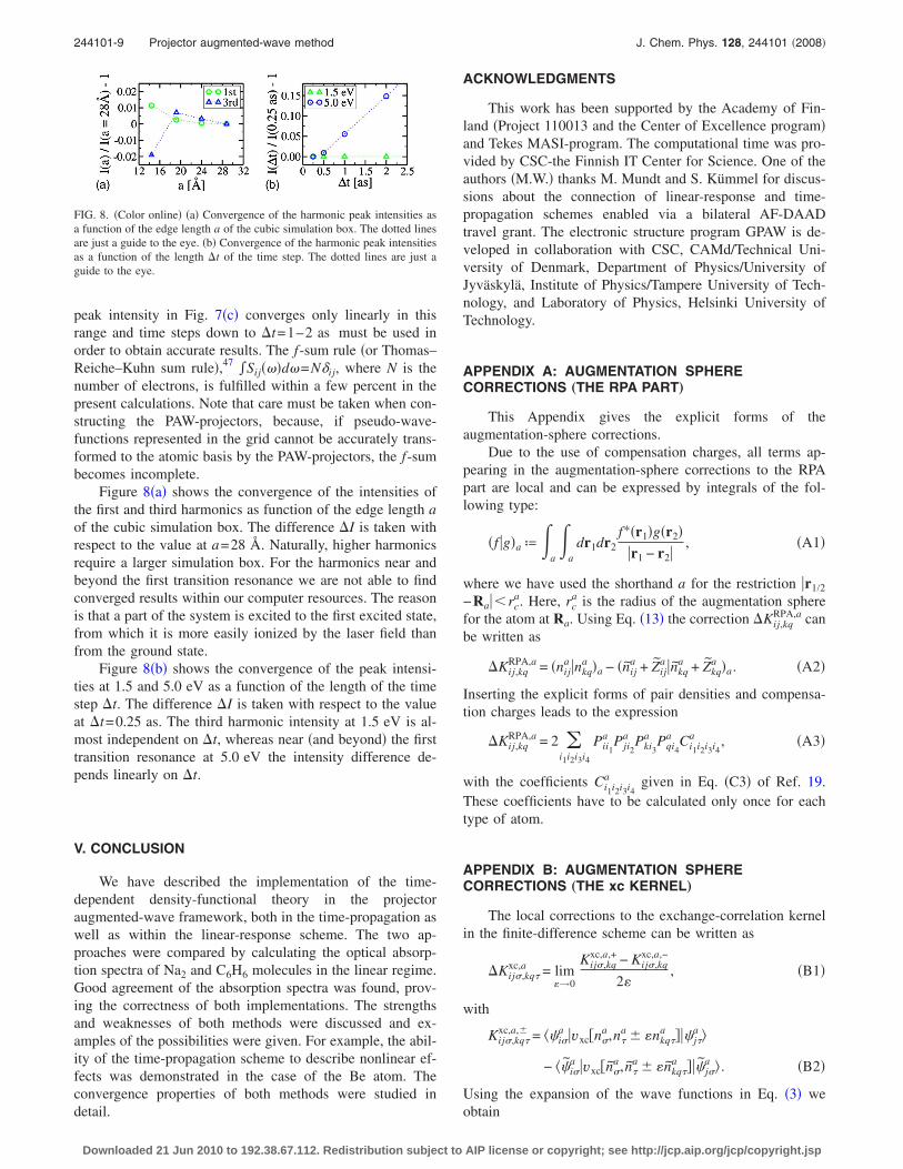
Figure 8�a� shows the convergence of the intensities ofthe first and third harmonics as function of the edge length aof the cubic simulation box. The difference �I is taken withrespect to the value at a=28 Å. Naturally, higher harmonicsrequire a larger simulation box. For the harmonics near andbeyond the first transition resonance we are not able to findconverged results within our computer resources. The reasonis that a part of the system is excited to the first excited state,from which it is more easily ionized by the laser field thanfrom the ground state.

Figure 8�b� shows the convergence of the peak intensi-ties at 1.5 and 5.0 eV as a function of the length of the timestep �t. The difference �I is taken with respect to the valueat �t=0.25 as. The third harmonic intensity at 1.5 eV is al-most independent on �t, whereas near �and beyond� the firsttransition resonance at 5.0 eV the intensity difference de-pends linearly on �t.

V. CONCLUSION

We have described the implementation of the time-dependent density-functional theory in the projectoraugmented-wave framework, both in the time-propagation aswell as within the linear-response scheme. The two ap-proaches were compared by calculating the optical absorp-tion spectra of Na2 and C6H6 molecules in the linear regime.Good agreement of the absorption spectra was found, prov-ing the correctness of both implementations. The strengthsand weaknesses of both methods were discussed and ex-amples of the possibilities were given. For example, the abil-ity of the time-propagation scheme to describe nonlinear ef-fects was demonstrated in the case of the Be atom. Theconvergence properties of both methods were studied indetail.

ACKNOWLEDGMENTS

This work has been supported by the Academy of Fin-land �Project 110013 and the Center of Excellence program�and Tekes MASI-program. The computational time was pro-vided by CSC-the Finnish IT Center for Science. One of theauthors �M.W.� thanks M. Mundt and S. Kümmel for discus-sions about the connection of linear-response and time-propagation schemes enabled via a bilateral AF-DAADtravel grant. The electronic structure program GPAW is de-veloped in collaboration with CSC, CAMd/Technical Uni-versity of Denmark, Department of Physics/University ofJyväskylä, Institute of Physics/Tampere University of Tech-nology, and Laboratory of Physics, Helsinki University ofTechnology.

APPENDIX A: AUGMENTATION SPHERECORRECTIONS „THE RPA PART…

This Appendix gives the explicit forms of theaugmentation-sphere corrections.

Due to the use of compensation charges, all terms ap-pearing in the augmentation-sphere corrections to the RPApart are local and can be expressed by integrals of the fol-lowing type:

�f �g�a ª a

a

dr1dr2f*�r1�g�r2�

�r1 − r2�, �A1�

where we have used the shorthand a for the restriction �r1/2−Ra��rc

a. Here, rca is the radius of the augmentation sphere

for the atom at Ra. Using Eq. �13� the correction �Kij,kqRPA,a can

be written as

�Kij,kqRPA,a = �nij

a �nkqa �a − �nij

a + Zija �nkq

a + Zkqa �a. �A2�

Inserting the explicit forms of pair densities and compensa-tion charges leads to the expression

�Kij,kqRPA,a = 2 �

i1i2i3i4

Pii1a Pji2

a Pki3a Pqi4

a Ci1i2i3i4a , �A3�

with the coefficients Ci1i2i3i4a given in Eq. �C3� of Ref. 19.

These coefficients have to be calculated only once for eachtype of atom.

APPENDIX B: AUGMENTATION SPHERECORRECTIONS „THE xc KERNEL…

The local corrections to the exchange-correlation kernelin the finite-difference scheme can be written as

�Kij�,kq�xc,a = lim

→0

Kij�,kqxc,a,+ − Kij�,kq

xc,a,−

2, �B1�

with

Kij�,kq�xc,a,� = ��i�

a �vxc�n�a ,n�

a � nkq�a ��� j�

a �

− ��i�a �vxc�n�

a , n�a � nkq�

a ��� j�a � . �B2�

Using the expansion of the wave functions in Eq. �3� weobtain

FIG. 8. �Color online� �a� Convergence of the harmonic peak intensities asa function of the edge length a of the cubic simulation box. The dotted linesare just a guide to the eye. �b� Convergence of the harmonic peak intensitiesas a function of the length �t of the time step. The dotted lines are just aguide to the eye.

244101-9 Projector augmented-wave method J. Chem. Phys. 128, 244101 �2008�

Downloaded 21 Jun 2010 to 192.38.67.112. Redistribution subject to AIP license or copyright; see http://jcp.aip.org/jcp/copyright.jsp

Kij�,kq�xc,a,� = �

iii2

Pi�i1Pj�i2

Ii1i2a,kq�,�. �B3�

Above, we have defined the integral

Ii1i2a,kq�,� =

a

dr��i1�r��i2

�r�vxc�n�,nkq�� �

− �i1�r��i2

�r�vxc�n�, nkq�� �� , �B4�

with the shorthands nkq� =n�

a�nkq�a and nkq

� = n�a�nkq�

a .Above, vxc depends on the modified atomic density matrixcompared to the Di1i2

a in Eq. �7�. A density change by �nkq�

results in a change in Di1i2a as

na�x� � nkqa �x� = � Di1i2,kq

a,� �i1a �x��i2

a �x� , �B5�

with

Di1i2,kqa,� = Di1i2

a �

2�Pki1

Pqi2+ Pki2

Pqi1� , �B6�

where we have used a symmetric notation to point out theexchange symmetry with respect to i1↔ i2. The integrals�Eq. �B4�� are evaluated numerically as described in Ref. 19.

1 W. Kohn and L. J. Sham, Phys. Rev. 140, A1133 �1965�.2 P. Hohenberg and W. Kohn, Phys. Rev. 136, B864 �1964�.3 E. Runge and E. K. U. Gross, Phys. Rev. Lett. 52, 997 �1984�.4 M. E. Casida, in Recent Developments and Applications in ModernDensity-Functional Theory, edited by J. M. Seminario �Elsevier, Amster-dam, 1996�, p. 391.

5 K. Yabana and G. F. Bertsch, Phys. Rev. B 54, 4484 �1996�.6 G. Senatore and K. R. Subbaswamy, Phys. Rev. A 35, 2440 �1987�.7 S. J. van Gisbergen, J. G. Snijders, and E. J. Baerends, Phys. Rev. Lett.

78, 3097 �1997�.8 J.-I. Iwata, K. Yabana, and G. F. Bertsch, J. Chem. Phys. 115, 8773�2001�, and references therein.

9 G. Onida, L. Reining, and A. Rubio, Rev. Mod. Phys. 74, 601 �2002�.10 R. Bauernschmitt and R. Ahlrichs, Chem. Phys. Lett. 256, 454 �1996�.11 A. Tsolakidis, D. Sánchez-Portal, and R. M. Martin, Phys. Rev. B 66,

235416 �2002�.12 N. L. Doltsinis and M. Sprik, Chem. Phys. Lett. 330, 563 �2000�.13 M. Moseler, H. Häkkinen, and U. Landman, Phys. Rev. Lett. 87, 053401

�2001�.14 X. Qian, J. Li, X. Lin, and S. Yip, Phys. Rev. B 73, 035408 �2006�.15 B. Walker and R. Gebauer, J. Chem. Phys. 127, 164106 �2007�.16 I. Vasiliev, S. Ögüt, and J. R. Chelikowsky, Phys. Rev. Lett. 82, 1919

�1999�.17 M. A. L. Marques, A. Castro, G. F. Bertsch, and A. Rubio, Comput. Phys.

Commun. 151, 60 �2003�.18 P. E. Blöchl, Phys. Rev. B 50, 17953 �1994�.19 J. J. Mortensen, L. B. Hansen, and K. W. Jacobsen, Phys. Rev. B 71,

035109 �2005�.20 See https://wiki.fysik.dtu.dk/gpaw.21 M. Casida, in Recent Advances in Density Functional Methods, Part I,

edited by D. Chong �World Scientific, Singapore, 1995�, p. 155.22 F. Furche, J. Chem. Phys. 114, 5982 �2001�.23 A. Putrino, D. Sebastiani, and M. Parrinello, J. Chem. Phys. 113, 7102

�2000�.24 D. Egli and S. R. Billeter, Phys. Rev. B 69, 115106 �2004�.25 M. Mundt and S. Kümmel, Phys. Rev. B 76, 035413 �2007�.26 T. Brabec and F. Krausz, Rev. Mod. Phys. 72, 545 �2000�.27 M. Protopapas, C. H. Keitel, and P. L. Knight, Rep. Prog. Phys. 60, 389

�1997�.28 W. H. Press, B. P. Flannery, S. A. Teukolsky, and W. T. Vetterling, Nu-

merical Recipes in C �Cambridge University Press, Cambridge, 1992�.29 A. Castro, M. A. L. Marques, and A. Rubio, J. Chem. Phys. 121, 3425

�2004�.30 R. Barrett, M. Berry, T. F. Chan, J. Demmel, J. Donato, J. Dongarra, V.

Eijkhout, R. Pozo, C. Romine, and H. V. der Vorst, Templates for theSolution of Linear Systems: Building Blocks for Iterative Methods, 2nded. �SIAM, Philadelphia, PA, 1994�.

31 J. P. Perdew and Y. Wang, Phys. Rev. B 46, 12947 �1992�.32 K. Huber and G. Herzberg, Constants of Diatomic Molecules, NIST

Chemistry WebBook, NIST Standard Reference Database Number 69,edited by P. J. Linstrom and W. G. Mallard �National Institute of Stan-dards and Technology, Gaithersburg MDY, 2003�. See http://webbook.nist.gov; data prepared by J. W. Gallagher and R. D. JohnsonIII.

33 W. R. Fredrickson and W. W. Watson, Phys. Rev. 30, 429 �1927�.34 S. P. Sinha, Proc. Phys. Soc., London, Sect. A 62, 124 �1949�.35 M. A. L. Marques, A. Castro, and A. Rubio, J. Chem. Phys. 115, 3006

�2001�.36 K. Yabana and G. F. Bertsch, Int. J. Quantum Chem. 75, 55 �1999�.37 I. Vasiliev, S. Ogut, and J. R. Chelikowsky, Phys. Rev. B 65, 115416

�2002�.38 S. Kotochigova, Z. Levine, E. Shirley, M. Stiles, and C. Clark, Atomic

Reference Data for Electronic Structure Calculations �National Instituteof Standards and Technology, Gaithersburg, MD, 2004�. Online available:http://physics.nist.gov/PhysRefData/DFTdata/contents.html.

39 E. J. Baerends, Phys. Rev. Lett. 87, 133004 �2001�.40 D. D. Konowalow, M. E. Rosenkrantz, and M. L. Olson, J. Chem. Phys.

72, 2612 �1980�.41 V. Bonacic-Koutecky, P. Fantucci, and J. Koutecký, J. Chem. Phys. 93,

3802 �1990�.42 H.-K. Chung, K. Kirby, and J. F. Babb, Phys. Rev. A 63, 032516 �2001�.43 W. J. Stevens, M. M. Hessel, P. J. Bertoncini, and A. C. Wahl, J. Chem.

Phys. 66, 1477 �1977�.44 T. Brabec and F. Krausz, Phys. Rev. 127, 1918 �1962�.45 R. W. Boyd, Nonlinear Optics, 2nd ed. �Academic, New York, 2003�.46 J. Fleming, M. R. Godefroid, K. L. Bell, A. Hibbert, N. Vaeck, J. Olsen,

P. Jonsson, and C. F. Fischer, J. Phys. B 29, 4347 �1996�.47 S. Wang, Phys. Rev. A 60, 262 �1999�.

244101-10 Walter et al. J. Chem. Phys. 128, 244101 �2008�

Downloaded 21 Jun 2010 to 192.38.67.112. Redistribution subject to AIP license or copyright; see http://jcp.aip.org/jcp/copyright.jsp